Multiple terms: term1 term2
red apples
returns results with all terms like:
Fructose levels in red and green apples
Precise match in quotes: "term1 term2"
"red apples"
returns results matching exactly like:
Anthocyanin biosynthesis in red apples
Exclude a term with -: term1 -term2
apples -red
returns results containing apples but not red:
Malic acid in green apples
hits for "" in
Network problems
Server timeout
Invalid search term
Too many requests
Empty search term
OPS4
This session focuses on the structure, dynamics, and evolution of these bodies, from surface to deep interior. We welcome contributions based on remote sensing, geological and geomorphological mapping, structural and tectonic analyses, stratigraphy, gravity and geophysical investigations, numerical and theoretical modelling, laboratory experiments, and comparative planetology. Studies addressing links between surface expression and internal processes, as well as long-term evolutionary pathways, are particularly encouraged.
Relevant targets include Io, Europa, Ganymede, Callisto, Enceladus, Titan, Triton, Pluto, and other outer Solar System moons and dwarf planets. Contributions based on data from past and ongoing missions, as well as studies supporting future exploration by Europa Clipper, JUICE, Dragonfly, and other upcoming missions, are strongly encouraged.
Introduction and Abstract
The RADAR instrument onboard the Cassini–Huygens spacecraft (2004–2017), operating at a wavelength of 2.2 cm, included both an active and a passive (radiometry) mode. In its active mode (as a Synthetic Aperture Radar), it measured the backscattered signal from the surface through the normalized radar backscatter cross section (σ0). In its passive mode, it recorded the surface microwave thermal emission through the measurements of the surface brightness temperature (Tb).
On November 6, 2011, the E16 flyby of Enceladus by the Cassini–Huygens spacecraft was dedicated to observations with the RADAR subsystem. During this flyby, the Cassini RADAR collected high-resolution observations of the South Polar Terrain (SPT) at its closest approach to Enceladus and medium-to-barely resolved observations of a combination of the moon leading and trailing hemispheres during the inbound/outbound legs of the flyby. Unfortunately, the inbound observations were contaminated by emission from Saturn and its rings, which laid behind Enceladus’ disk during the acquisition. Therefore, this study focuses on two sets of data (1) High-resolution SAR and Tb maps obtained close to the tiger stripes region (2) Four radiometry segments acquired during the E16 outbound leg at mid-latitudes and with a moderate spatial resolution.
Both resolved and unresolved observations of Enceladus have consistently highlighted its extremely high radar-brightness, the highest in the Solar system [1,2]. Radiometry observations along the E16 swath revealed thermal anomalies that had not been detected in the infrared [3]. However, the magnitude of the internal heat flux remained to be constrained.
In this study, we performed the re-analysis of the high-resolution datasets collected over the SPT and obtained constraints on structural, chemico-physical and thermal state of surface and subsurface, including parameters such as grain size, porosity, the presence of water-ice/dust contaminants, and endogenic heat flux [4]. These results have important implications for future missions to Enceladus, in particular for potential lander missions targeting its south polar region.
A portion of the mid-resolution datasets was previously analyzed in a qualitative manner by [5], revealing a large-scale emissivity anomaly in Enceladus’ Leading Hemisphere Terrain (LHT). This region is interpretated to be relatively young, potentially reflecting recent of the resurfacing processes, in agreement with the structural and geological mapping of Enceladus by [6]. The emissivity anomaly is also explained by a scattering anomaly. However, the nature and origin of the observed scattering/emissivity anomalies (such as the characteristic size of the scatterers or the depth of emission) remain unconstrained. The objective of the present re-analysis of the E16 dataset is therefore to better constrain these properties, in order to improve our understanding of the surface phenomena behind such anomalies and, more broadly, the evolutionary history of Enceladus.
Methodology
To predict backscatter (σ0) and thermal emission in the microwave domain we combine two models: (1) a thermal model providing depth profiles of the physical temperature beneath the surface at E16 flyby epoch, (2) a radiative transfer model to simulate both active and passive observations.
Thermal Model: We adapted a multi-layer thermal model called MultIHeaTS [7] to the case of Enceladus. We account for Solar flux and radiative flux equilibrium at surface and a constant temperature or a zero-temperature gradient at the bottom. The subsurface of Enceladus is modeled as mono or bi-layer medium (with an icy porous regolith overlying a denser water ice substrate).
Radiative Transfer Model: We use Snow Microwave Radiative Transfer (SMRT) model, a multi-layer RT model initially designed for snow or sea-ice [8]. Permittivity of water ice is assumed constant with temperature [9], effective permittivity depends on its porosity and includes possible contaminants fraction, assumed as organic dust. The parameters of RT model are thus the dust fraction and water ice grain radius size.
Results
1. SPT observations
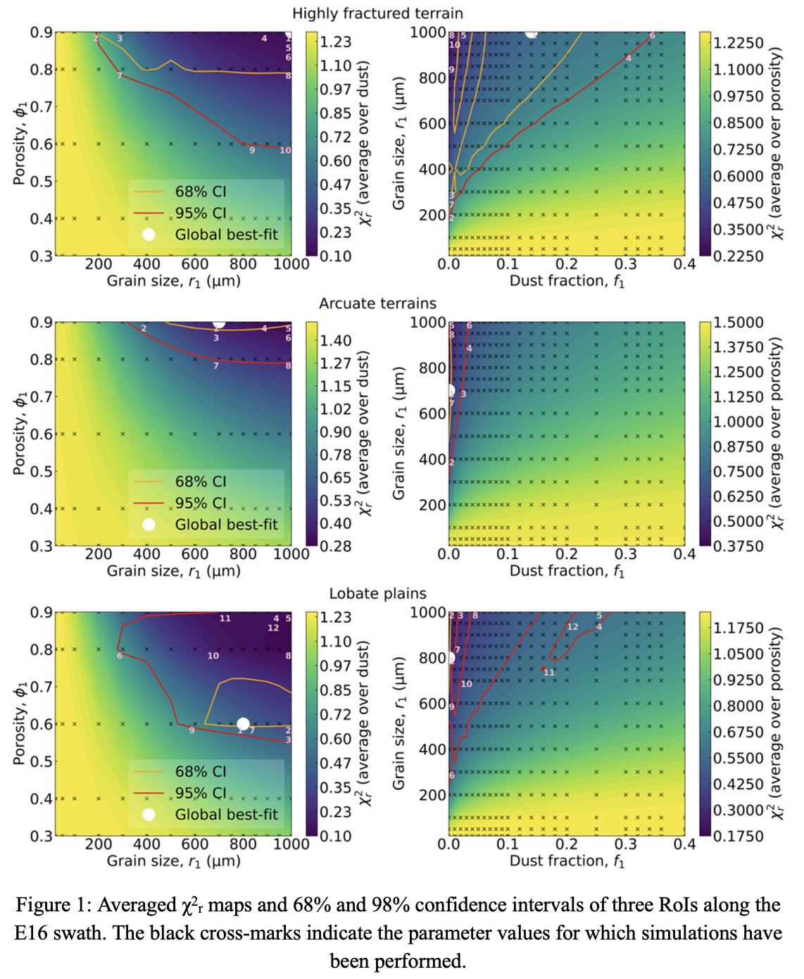
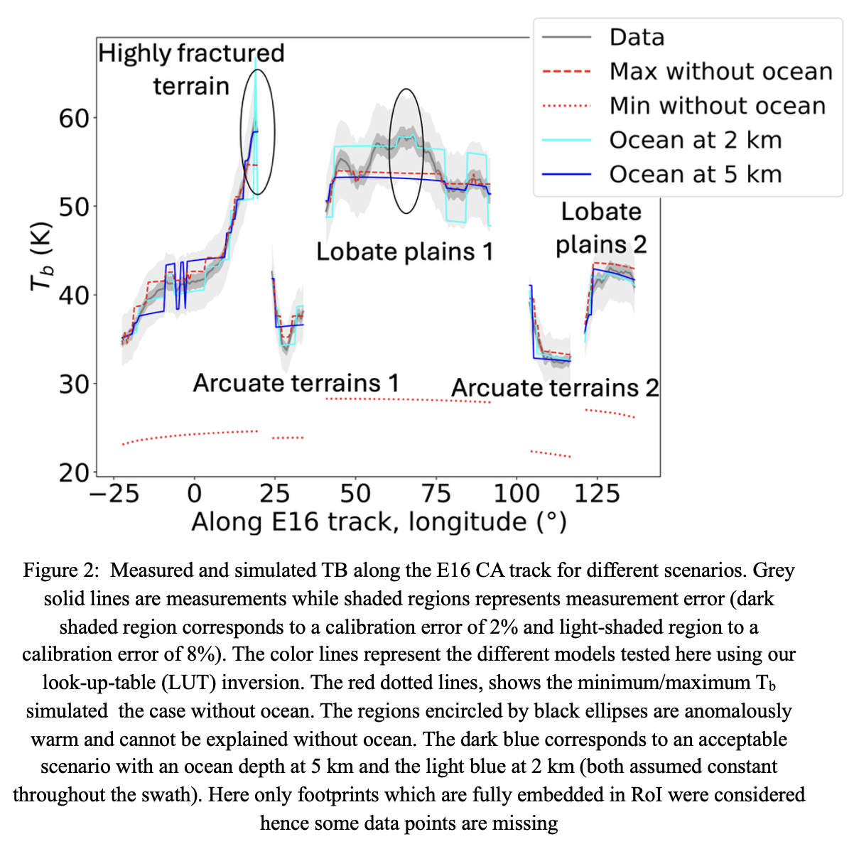
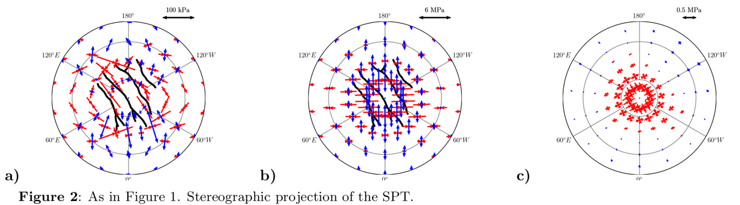
The inversion results suggests that the regolith is characterized by relatively large scattering structures (>500 µm), limiting radar sensitivity to the upper few meters. They also indicate that regolith purity and porosity vary with local geology and between the different identified RoIs (see Figure 1). The anomalously radar bright regions are covered with pure and highly porous water ice. Anomalously high Tb values observed over parts of the swath can only be explained by the presence of an ocean at shallow subsurface (2-5 km deep), associated with enhanced heat loss (up to 900 mW/m2). However, due to degenericies between parameters, the non-anomalous Tb observations can also be explained without invoking a subsurface ocean (see Figure 2). These results are described in details in [4].
2. LHT observations
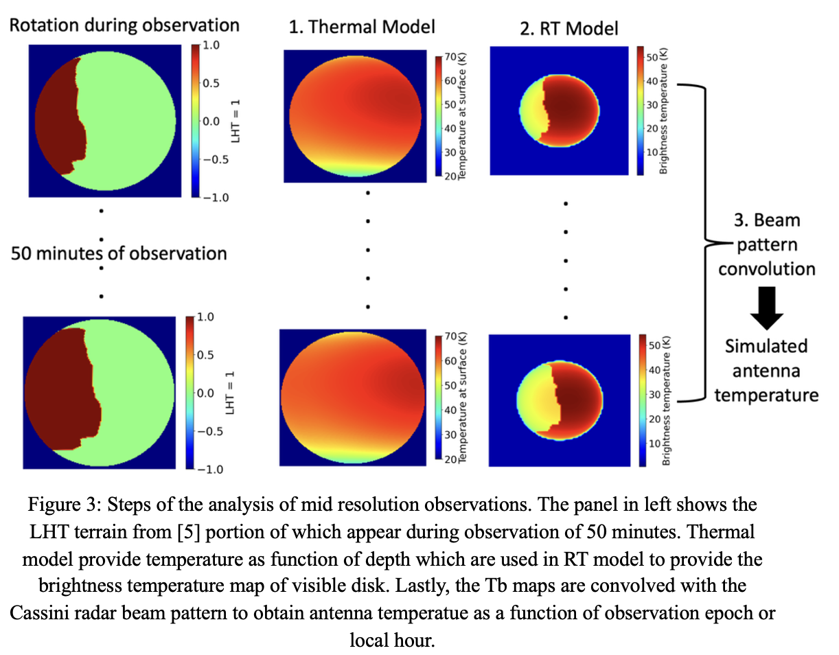
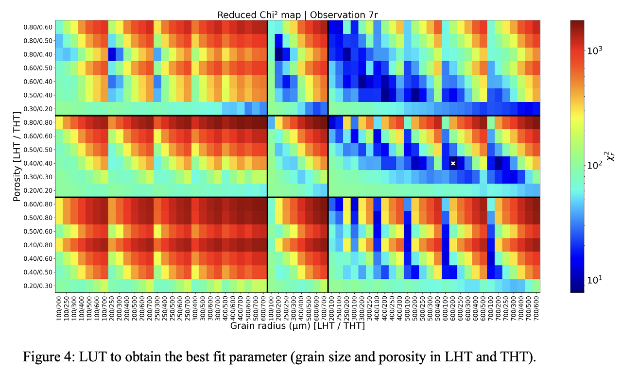
Here we present the ongoing re-analysis of of mid-resolution dataset, building on the work of [4]. Figure 3 displays the schematic of data-to-model comparison workflow. During the outbound leg, as the spacecraft was moving away from the target, the rotation of the moon is taken into account. We first consider a simple mono-layer medium for the subsurface, with no-ocean at bottom and consisting of pure water ice. The properties are varied between the LHT and THT including the cases when both terrains share same properties. Our preliminary inversion results show that: (1) reproducing the emissivity anomaly over the LHT required either higher porosity, or larger grain size (2) there are degeneracies between the parameters - porosity and grain size (see Figure 4). Nevertheless, the best fit solution indicates that the observed anomalies are not related to a change in thermal inertia, but are instead primarily driven by variations in grain size (i.e., scattering and emissivity effects). Finally, results obtained with a bi-layer model (both for the LHT and THT) results will be presented, as this assumption may provide a better explanation of the observations. In addition, the bi-layer approach should put constraints on the depth of emission anomaly.


How to cite: Raza, M. S., Le Gall, A., and Schmidt, F.: Investigation of the South Polar Terrain and Leading Hemisphere of Enceladus using the Cassini RADAR observations, Europlanet Science Congress 2026, The Hague, The Netherlands, 7–11 Sep 2026, EPSC2026-259, https://doi.org/10.5194/epsc2026-259, 2026.
Jupiter’s moon Ganymede, the largest moon in the Solar System, is the main focus of the JUICE mission, which will observe its surface and measure its interior with unprecedented detail (Van Hoolst et al., 2024). In contrast with smaller moons such as Europa or Enceladus where an ocean is in contact with the silicate interior, Ganymede contains a high pressure (HP) ice layer between its ocean and the rocky core. Thus, on Ganymede, the dynamics in the high pressure ice layer control the exchange of heat and chemical species between the ocean and rocky interior.
The thickness of the HP ice layer is not well constrained, and interior structure models suggest thicknesses around 400 km, with values as low as 100 km (Kalousova et al., 2018) and as high as 700 km (Vance et al., 2018). Depending on the thickness of this layer, various high-pressure ice polymorphs might appear (Hussmann et al., 2015), such as ice V and ice VI, and for a sufficiently cold ocean also ice III (Journaux et al., 2020). Here we focus on ice V and ice VI, as they might exhibit different viscosities that in turn can substantially affect the convective behavior of the HP ice layer. Rheological experiments of ice V and ice VI are rare, but existing studies (Sotin & Poirier, 1987) indicate that ice V can be harder to deform than ice VI, and the viscosity ratio can reach up to three orders of magnitude.
Model
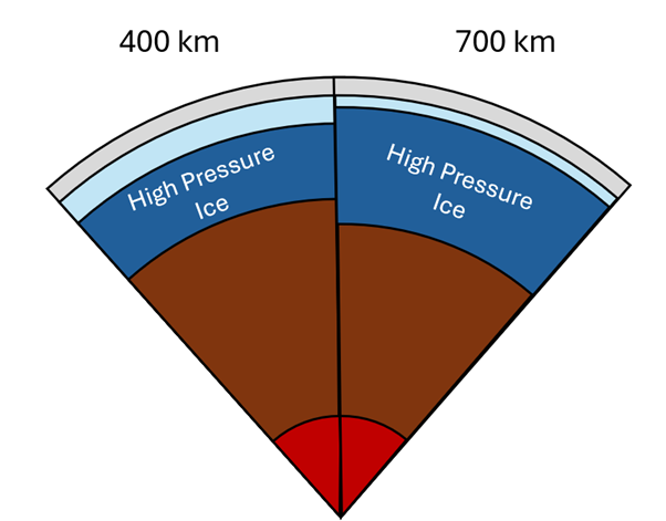
We investigate the dynamics of Ganymede’s HP ice layer using the geodynamical code GAIA (Hüttig et al., 2013). GAIA numerically solves the conservation equations of mass, linear momentum and thermal energy in 2D and 3D geometries. Our models use free-slip boundary conditions at the ice-ocean interface and no-slip at the boundary between the high-pressure ice layer and the silicate interior. The temperature is set at the melting temperature of water ice at the ice-ocean interface, while for the ice-silicate boundary we prescribe a heat flow that decreases with time from 20-40 mW/m2 at 4.5 Gyr ago to 5-10 mW/m2 at present day, values that have been used in previous studies (Choblet et al., 2017). Since the thickness of the high pressure ice layer on Ganymede is poorly constrained we test models with 400 km and 700 km (Fig. 1).

Fig. 1: Thickness and structure of the high pressure ice layer tested in this study.
Our models use the viscosity formulation of Kalousová et al. (2018) that has been derived from rheological experiments (Sotin et al., 1985; Durham et al., 1996). This Arrhenius-type relation expresses viscosity as a function of temperature difference from the local pressure-dependent melting point, such that ice has a higher viscosity when the temperature is away from the melting curve and lower as it approaches it. The melting curve is pressure-dependent and differs for the high pressure ice phases (Chizov, 1993). We test models where the HP ice layer of Ganymede is subdivided into ice V and ice VI layers. Our models vary the reference viscosity of the ice VI layer between 1015 and 1018 Pa s and apply a viscosity contrast between the ice V and ice VI layers of up to 1000. Similar to Choblet et al. (2017), we limit the temperature to the melting temperature of the HP ice layers and compute the amount of melt produced throughout the evolution.
Results and Discussion
Our models show that the ice shell dynamics substantially change with both the reference viscosity and the increase of viscosity contrast between ice V and ice VI. In the early evolution, a lower reference viscosity leads to vigorous convection in the high pressure ice layer and efficient cooling. By present day this trend reverses, with higher reference viscosity models remaining more convective and warmer. Introducing a viscosity contrast between ice V and ice VI increases the vigor of convection, both in the early evolution and at present day. A high contrast in viscosity between ice V and ice VI (i.e., two orders of magnitude or more) also leads to the development of a two-layered convection structure. Convection is concentrated in the lower ice VI layer, while the upper ice V layer acts as a stiff lid. Heat and material transport from the ice-rock interface to the ocean occurs in pulses, when convective plumes penetrate through this high-viscosity ice V layer.
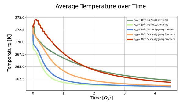
Melt production is most significant during early evolution, when the temperature in the high pressure layer is high. For models with a high viscosity contrast between ice V and ice VI layers, the temperatures are higher compared to cases without a viscosity jump (Fig. 2). This is a consequence of sluggish convection in the ice V layer and, hence, less efficient cooling. As a result, more melt is produced over the full evolution when a high viscosity contrast is applied (i.e., the melt volume is three times higher for a model with a 400 km ice shell thickness and three orders of magnitude viscosity contrast compared with a model without a viscosity jump).
We note that the 400 km ice shell models are warmer than the 700 km models, given their slightly higher temperature at the ice-ocean interface (265 K vs. 248 K) and their larger ice-silicate contact area. In the absence of tidal heating, the models with an ice shell thickness of 400 km receive more heat through the bottom boundary than the 700 km models. In addition, more vigorous convection in the 700 km cases leads to stronger cooling through time. The higher ice shell temperatures also lead to a larger amount of melt (about two to four times larger) that can be produced in the 400 km cases compared to the 700 km simulations.
Future models will include the effects of tidal heating and track the redistribution of impurities, i.e., salts, through the high pressure ice layers of Ganymede.

Fig. 2: Evolution of the average temperature in the high pressure ice shell of Ganymede for various rheological structures.
How to cite: van den Heuvel, N., Plesa, A.-C., Hussmann, H., and Sotin, C.: Dynamics and Evolution of the High Pressure Ice Layer on Ganymede, Europlanet Science Congress 2026, The Hague, The Netherlands, 7–11 Sep 2026, EPSC2026-980, https://doi.org/10.5194/epsc2026-980, 2026.
Introduction
With its geologically young surface crosscut by linear structures such as ridges, lineae, and bands, Europa is a unique moon in our Solar System. It has been explored by multiple spacecraft, in particular the Galileo mission, which inferred the existence of a subsurface salty ocean, as well as the presence of surface salts, likely MgSO4 [1]. The Hubble Space Telescope also identified irradiated NaCl, which is consistent with the reddish color of Europa [2]. Their distribution across the surface coincides with geological structures, suggesting an internal origin and exchange of non-ice material (NIM) with its interior [1]. Europa undergoes periodic eccentricity variations over cycles of hundreds of million years [3], leading to global compression and extension [4,5]. As a result, the ice shell exhibits significant thickness variations, ranging from ~3-10 km to ~60-70 km [3,4,5].
Unraveling the formation of dilational bands is a key to a better understanding of Europa's history. These wide bands, extending for hundreds of kilometers across its surface, are characterized by a complete opening of the surface with exposure of subsurface material in the fault zone. Their morphology suggests an extensional origin, and they likely form during the thickening of the ice shell [6,7]. Most of them spread from a V-shaped central trough, are roughly symmetrical, and often elevated with respect to surrounding terrains [6,7,8]. They exhibit a moderate topography of a few hundred meters [6,8,9] and are commonly classified into four main categories, depending on their brightness and texture [7]. Dark bands are the most common and are inferred to be richer in non-ice materials (NIM) and younger than bright bands [6,9]. Bright bands, on the contrary, are usually older, and often flanked by darker material [6,7,8]. Smooth bands have a hummocky texture with small-amplitude oscillations [7,8], while lineated bands consist of regularly spaced sub-parallel ridges and faults, spreading symmetrically from the central depression [6,7,8].
We aim to unravel the conditions under which these bands are formed. We investigate the effect of various parameters, such as the ice shell thickness D, extension velocity Vext, ice cohesion Cice, and grain size, on band morphology and topography, using a two-dimensional Cartesian model of the ice shell undergoing a constant strain-rate tectonic extension. We also seek to investigate how tectonic extension drives transport of NIM and oceanic material to the surface, as well as their distribution.
Results
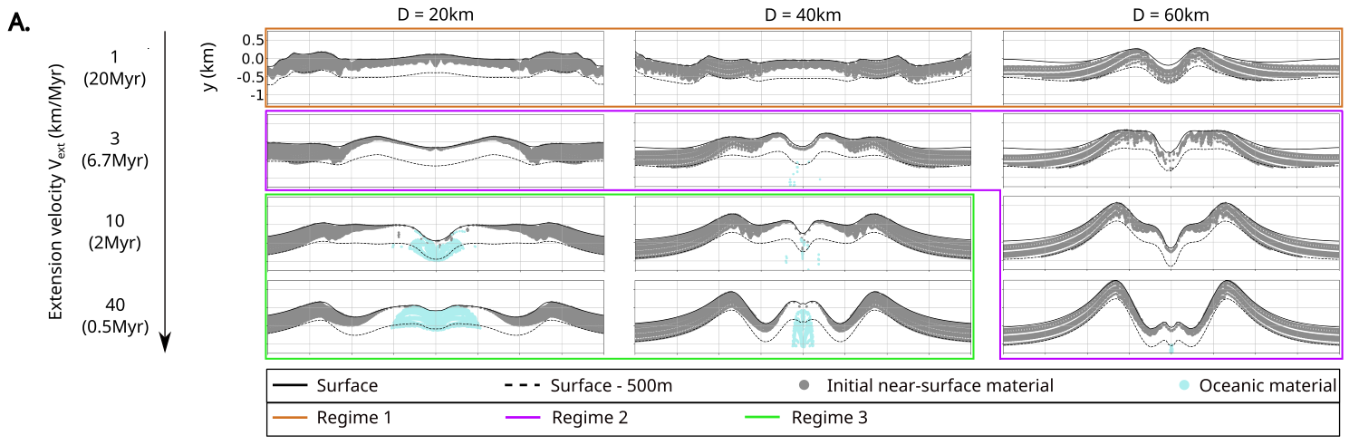
Several parameters significantly affect the formation of dilational bands, particularly Vext and D. We identify three main dynamical regimes, controlled by the efficiency of surface opening (Fig.1). Complete surface opening occurs only for sufficiently high strain rates, on the order of 10 km.Myr−1, and is further enhanced for thinner ice shells. The third regime is therefore the most consistent with dilational band formation (Fig.1).
Efficient surface opening also promotes mass exchanges, with higher strain rates favoring the exposure of oceanic material at the surface. Thinner ice shells further enhance the exposure of oceanic material within the fault zone (Fig.2B). In these cases, NIM are pushed away from the fault zone. One important result is that the final lateral distribution across the band reflects the initial vertical distribution of material within the ice shell.
Another key parameter is Cice, which controls the strength of the lithosphere. Fig.2 illustrates the effect of Cice on band formation for two different ice shell thicknesses. Tectonic extension commonly drives local convection within the ice shell, enhancing mass exchanges with the surface (Fig.2A). The strength of the lithosphere strongly affects band morphology, particularly the symmetry of the structure and the presence of a distinct central trough (Fig.2).
Conclusion
We suggest that various types of bands were formed during distinct extensional events, explaining their brightness and texture differences. In particular, bright bands may form at an early stage of ice shell thickening when a thinner ice shell promotes the exposure of oceanic material within the fault zone. This provides a consistent explanation for their bright central region and often darker edges enriched in NIM. These darker edges may also result from a longer radiation exposure. In most cases, the farther from the center of the domain, the longer the material has remained at the surface, exposed to radiation (Fig.2C). In contrast, dark bands may form later, when the ice shell is thicker, limiting the exposure of oceanic material and resulting in a higher fraction of NIM within the fault zone. Finally, we are able to predict the morphology and composition of the dilational bands based on the rheological and physical properties of the ice shell at the time of extension. We show that we can also constrain the initial vertical profile in the ice shell from the vertical distribution of material across the band.
Figure 1 - Effect of D and Vext on the final distribution of initial near-surface material and exposure of oceanic material.
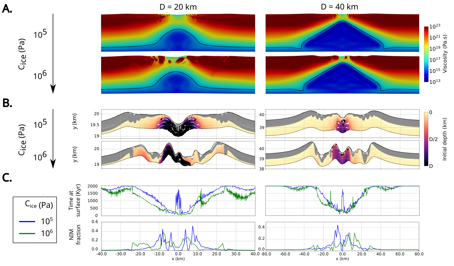
Figure 2 - Effect of Cice and D on: A. the viscosity field at the end of the extension, and B. the initial depth of the post-extension near-surface material. Grey part corresponds to what remains of the initial near-surface material. C. Comparative plots for two values of Cice: average time spent in the topmost cell by post-extension near-surface material, and fraction of NIM at the surface at the end of the extension.
References
[1] R. Carlson et al. (2009), In Europa, eds. R. T. Pappalardo et al., 283–327
[2] S. K. Trumbo et al. (2019), Sci. Adv., 5, eaaw7123
[3] H. Hussmann and T. Spohn (2004), Icarus, 171, 391-410
[4] M. L. Rudolph et al. (2022), Geophys. Res. Lett., 49(5), e2021GL094421
[5] M. Kihoulou et al. (2025), Sci. Adv., 11, eadq8719
[6] L. Prockter et al. (2002), J. Geophys. Res. Planets, 107(E5), 5028
[7] L. Prockter and G. Patterson (2009), In Europa, eds. R. T. Pappalardo et al., 237-258
[8] B. Tufts (2000), Icarus, 146, 75-97
[9] F. Nimmo et al. (2003), Geophys. Res. Lett., 30(5), 1233
How to cite: Lebec, L., Kihoulou, M., Čadek, O., Tobie, G., and Choblet, G.: Cracking Europa: Dilational bands formation and material transport in the ice shell, Europlanet Science Congress 2026, The Hague, The Netherlands, 7–11 Sep 2026, EPSC2026-100, https://doi.org/10.5194/epsc2026-100, 2026.
Introduction
Among the icy satellites of Uranus, Ariel is considered a candidate ocean world [1]. The available imagery of the surface by Voyager 2 covers less than 40% of its surface [2], from which mosaics and digital elevation models (DEM) were produced [3]. Spectral information of Ariel’s surface indicates a composition mainly of H2O, CO2, and CO ices [4], and an interpretation of James Webb Space Telescope (JWST) observations [5, 6] suggests the presence of nitrogen-bearing species. In addition, a geological map of the imaged region has been produced and digitized [7, 8] and later combined with relative and absolute age estimates for the youngest and oldest geological units [9]. These studies indicate that Ariel underwent extensive resurfacing not later than 3.0 Ga. Altogether, this makes Ariel a compelling target for investigating the origin and morphology of its extensional features. In this work, we estimated the geometrical parameters of the main chasmata to evaluate the extension of the visible area.
Data and Methods
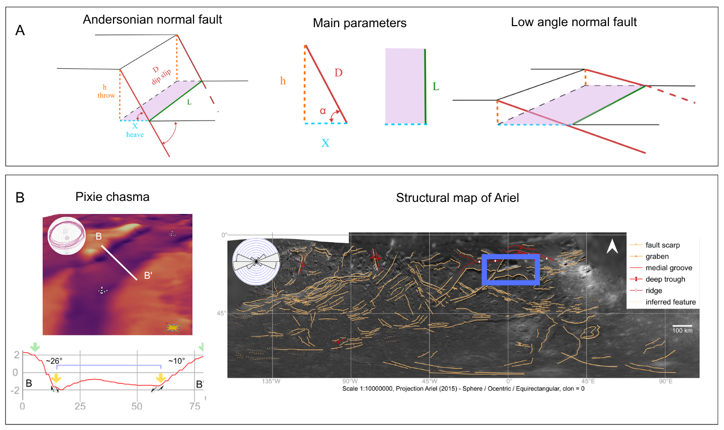
We used DEMs, photomosaic, and the structural map based on Voyager 2 data [2,10] (Fig.1B). After conducting the structural analysis of the surface, we developed a pipeline to evaluate the geometrical parameters of the chasmata. The length distribution of features was studied to identify the spacing pattern [11]. The geometries of the biggest chasmata have been assessed to establish relationships between length and vertical displacement [12]. The vertical displacement was calculated from measurements of throw. Extension area (A) was calculated using the formula: A = L/tan(α) [13], where L is the length of a chasma and α is a dip angle (Fig.1A).

Figure 1. A. Schematic model of a normal fault with a dip angle of 60 degrees, illustrating the key geometrical parameters used for extension area estimation: h (throw), X (heave), L (length), D (vertical displacement), and dip angle (α). On the right side of panel A, an example of a normal fault with a low dip angle and its extension area is shown. B. Three-dimensional view of Pixie Chasma with a stereoplot of dip measurements obtained in VRGS[14], alongside a geological profile displaying average dip angles on each side. Yellow and green arrows indicate the marginal trough and chasma rim, respectively. The structural map of Ariel features a Rose diagram [15] indicating the orientations of structures. The blue rectangle marks the location of Pixie Chasma.
Discussion and future work
Dip angle estimations of the main chasmata reach 50 degrees at maximum and around 25 degrees on average, lower than the typical angle of 60 degrees for an Andersonian fault assumed before [16, 17]. Even though the interpretations of dip angle values should be taken cautiously because of the DEM medium quality, the low values of dip can significantly increase the amount of extension. Overall, these estimates suggest a sensibly higher radius change of the whole body connected to chasmata formation and development unless compensated by other processes. From a morphological point of view, the dip measurement could also be affected by slope deposits, which could have been overlooked due to poor resolution. New missions collecting high-resolution imagery will significantly improve the analysis.
Acknowledgements: This activity has been developed under the ASI/UniBo-CIRI agreement n. 2024-5-HH.0.
References:
[1] Castillo‐Rogez J. et al. (2023) J. Geophys. Res. Planets e2022JE007432. [2] Schenk P.M. and Moore J.M. (2020) Philos. Trans. R. Soc. A 20200102. [3] Beddingfield C.B. et al. (2025) Planet. Sci. J. 32. ad9d3f. [4] Cartwright R.J. et al. (2015) Icarus 257, 428-456. 2015.05.020. [5] Cartwright R.J. et al. (2020) Astrophys. J. Lett. L22. aba27f. [6] Cartwright R.J. et al. (2024) Astrophys. J. Lett. L29. [7] Croft S.K. and Soderblom L.A. (1991) Uranus 561-628. [8] Beddingfield C.B. and Cartwright R.J. (2021) Icarus 114583. [9] Kirchoff M.R. et al. (2022) Planet. Sci. J. 42. ac42d7. [10] Tonoian S. et al. (2025) EPSC-DPS2025-1554. 1554. [11] Soliva R. and Schultz R.A. (2008) Tectonics 27. 2007TC002148. [12] Schultz R.A. and Fossen H. (2002) J. Struct. Geol. 24, 1389-1411. S0191-8141(01)00146-8. [13] Golombek M.P. (1982) J. Geophys. Res. Solid Earth A77-A83. JB087iS01p00A77. [14] VRGeoscience Limited (2003) VRGS. Retrieved from: www.vrgeoscience.com. [15] Alberti M. et al. (2016) Rendiconti Online Soc. Geol. Ital. 39, 55-59. [16] Bergstralh J.T. et al. (1991) Uranus. [17] Watters T.R. and Schultz R.A. (2010) Planetary tectonics. Cambridge University Press.
How to cite: Tonoian, S., Lucchetti, A., Massironi, M., Penasa, L., Beddingfield, C., Pajola, M., Rossi, C., and Pozzobon, R.: Geometry of chasmata on Ariel’s surface and its implications, Europlanet Science Congress 2026, The Hague, The Netherlands, 7–11 Sep 2026, EPSC2026-490, https://doi.org/10.5194/epsc2026-490, 2026.
Estimating surface properties such as porosity and grain sizes is key for planning lander missions and landing site selection on icy moons. However, spaceborne instruments do not measure the regolith properties directly: instead, they record proxy measurements such as thermal flux, which are then interpreted through modeling to estimate thermal inertia, porosity, grain size, etc.
A striking conclusion from all thermal measurements that probed the uppermost surface (first millimeters) of icy moons is they all show an exceptionally low thermal inertia, ranging from 9 to 20 J·m⁻²·K⁻¹·s⁻¹/². This value is orders of magnitude lower than that of bulk hexagonal water ice (2000 J·m⁻²·K⁻¹·s⁻¹/²) at these temperatures. We demonstrate that a regolith thermally dominated by hexagonal water ice may only achieve such thermal inertia through a combination of extremely high porosity (>80%), small grain radii (<1 mm), and an unconsolidated regolith (minimal contact area between grains), consistent with previous photometry and spectroscopy studies.
For the Galilean moons, deeper thermal observations (>1 cm) have revealed higher thermal inertia (>~50 J·m⁻²·K⁻¹·s⁻¹/²), indicating that the regolith compacts over centimeter scales. Since gravity has no effect on compaction on such scale, we propose three formation scenarios to account for vertical layering: deposition cover, degradation by impactors, and temperature gradient metamorphism.
We discuss how monodisperse grains can reach such extreme porosities and provide examples of experimental analogs that could best represent the regolith. We propose that high porosity regolith are favored on icy moons due to the adhesive nature of water ice and their low-gravity environment.
How to cite: Mergny, C., Cornet, T., Le Gall, A., Cruz-Mermy, G., Lange, L., Rückriemen-Bez, T., Gundlach, B., Heitmann, P., Goldmann, M., O. Hayne, P., and Oza, A.: What does the regolith of icy moons look like?, Europlanet Science Congress 2026, The Hague, The Netherlands, 7–11 Sep 2026, EPSC2026-335, https://doi.org/10.5194/epsc2026-335, 2026.
The Visual and Infrared Mapping Spectrometer (VIMS) onboard Cassini collected thousands of spatially resolved spectra of the surface of the five inner mid-sized moons of Saturn (Mimas, Enceladus, Tethys, Dione and Rhea) between 2004 and 2017 [1]. These moons are embedded in Saturn’s E-ring, generated by Enceladus’ plumes and containing water ice grains, either in pure form or contaminated by organics or salts [2]. The mid-sized moons are characterized by an icy surface affected by endogenous activity and exogenous processes, such as cratering events, UV irradiation, accumulation of E-ring particles, and weathering from the interaction with energetic particles [3]. Their surfaces are darkened by agents that could be the same over the whole Saturn system, yet there is no consensus to date on their exact nature [4]. To explain the observed reddening and darkening of Saturn’s inner moons, it has been suggested that their surfaces may be impacted by processed organic-rich E-ring grains, thought to get redder and darker upon irradiation at the moon’s surface, and during their travel from Enceladus to the moons [3]. In this study, we aim to test this hypothesis by performing radiative transfer modeling of Dione’s surface.
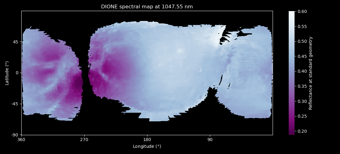
Exploiting the VIMS dataset and relying on previous works [1,5], we produced photometrically corrected maps of Dione, for the first time at full VIMS spectral coverage. We used a photometric correction method based on the Akimov theory [1] to independently convert all the VIMS-VIS and VIMS-IR spatially resolved spectra to the same illumination condition (incidence angle and phase angle of 30°, emission angle of 0°). Implementing new filtering steps, we cleaned the dataset from pixels with irregular photometric responses (saturated or partially-filled pixels), to improve the quality of the spectral maps. Then, using the produced filtered dataset of photometrically corrected spectra, we produced spectral maps of Dione by projecting each pixel and their corresponding spectrum on a cylindrical map of the moon’s surface, according to the pixel’s average position in latitude and longitude. We calculated the median spectrum of each tile of the map at each wavelength, using a sampling of 2 pixels per degree. Finally, we produced the full VIS-IR spectrum of each pixel at the surface of Dione, by bridging the VIS and IR spectra. Fig.1 shows the final spectral map obtained for Dione at a wavelength around 1047 nm.

Fig.1: Spectral map of Dione at 1047.55 nm. The high albedo contrast between the leading and trailing hemispheres is well appreciated, as well as the presence of several craters, and bright faults across the moon’s trailing hemisphere (nicknamed ‘wispy terrains’).
To further characterize the moon’s surface and to derive estimates of the composition and physical properties of its different regions, we performed spectral unmixing by applying a well-tested simplified Hapke Isotropic Multiple Scattering Approximation (IMSA) model [5,6]. Such modeling is performed for the first time in a systematic way across the whole surface of Dione, so that the produced compositional maps can be used to better understand the surface distribution of the contaminants with respect to the processes altering Dione's surface. Hapke theory allows for the computation of the reflectance of a given mixture of components as a function of their optical constants. Dione is known to be covered in water ice of different grain sizes, affected by darkening agents. In our model, we assume tholins as the agents responsible for Dione’s surface reddening, as they are considered a good proxy of the organic residues produced by irradiation of icy surfaces [5]. Furthermore, we consider amorphous carbon as a neutral absorber responsible for the lowering of the surface albedo and the reduction of the depth and contrast of water ice absorption bands [5]. We thus considered four different populations of components: (i) large water ice grains (≥µm) mixed with tholins in an intra-particle mixture; (ii) sub-µm water ice grains; (iii) sub-µm amorphous carbon grains; and (iv) large water ice grains mixed with sub-µm amorphous carbon grains in an intra-particle mixture. The best fit of each pixel of the moon's map has been achieved using a Levenberg-Marquardt (LM) least squares algorithm. In order to sample the parameter space, we varied the grain sizes, abundance and fraction of contaminants in the water ice grains.
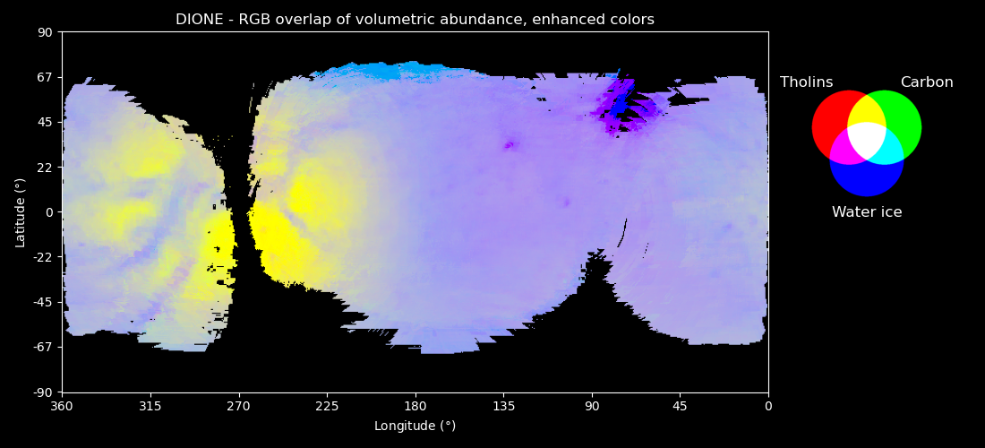
A resulting optical abundance map of Dione is shown in RGB colors in Fig.2. We can observe that tholins and carbon are both more abundant in the trailing hemisphere of the moon, while its leading hemisphere is coated in purer water ice. The competition between different exogenous processes such as E-ring particles deposition and cold plasma particles bombardment are currently under study, in order to assess the consistency of our results with the hypothesis tested in this work [3].

Fig.2: Dione RGB overlap of the volumetric abundance of water ice (blue), of tholins (red) and of amorphous carbon (green). The colours corresponding to the abundance of tholins and amorphous carbon have been boosted for a better visual representation.
[1] Filacchione, G., et al., Icarus 2022, 375.
[2] Postberg, F., et al., 2018. in Enceladus and the Icy Moons of Saturn, ed. P. M. Schenk, R. N. Clark, C. J. A. Howett, A. J. Verbiscer, & J. H. Waite, p.129
[3] Hendrix, A.R., et al., 2018. Icarus 300, 103-114
[4] Clark, R.N., et al., Icarus 2008, 193, 372–386.
[5] Ciarniello, M., et al., Icarus 2011, 214, 541–555.
[6] Hapke, B., 2002. Icarus 157, 882, 523–534.
Acknowledgements: This work is supported by the INAF data analysis grant “Mid-sized Saturnian icy Satellites Investigation by Spectral modeling” (MISSIS) and by the project "Preliminary study of payloads for missions to Saturn's moon Enceladus" ASI--INAF agreement n. 2024-19-HH.0.
How to cite: Galinier, M., Ciarniello, M., Filacchione, G., Raponi, A., Galluzzi, V., D'Aversa, E., and Gorga, B.: Study of the darkening agents of Saturn's mid-sized icy moon Dione, Europlanet Science Congress 2026, The Hague, The Netherlands, 7–11 Sep 2026, EPSC2026-494, https://doi.org/10.5194/epsc2026-494, 2026.
The Juno mission, through its JIRAM infrared instrument, has fundamentally reshaped our understanding of Io, transitioning our view of the moon from a collection of isolated hotspots to a world dominated by interconnected magmatic systems. This presentation synthesizes key findings from the 2023–2024 close flybys, which provided unprecedented spatial resolution of Io’s volcanic landscapes.
JIRAM observations have confirmed that lava lakes are the most ubiquitous volcanic feature on Io, typically characterized by a cooling central crust surrounded by a narrow "hot ring" of exposed lava. A critical shift in our understanding of Io’s energy budget has emerged: while these rings are the most prominent features in the M-band (5 µm), the vast majority of the total thermal power is actually emitted by the larger, low-temperature crusts. This implies that previous observations, insensitive to these cooler components, may have underestimated the contributions of lava lakes to Io’s volcanic heat flow by up to an order of magnitude; we identified crustal overturn in paterae as a primary cooling mechanism for the interior.
How to cite: Mura, A., Tosi, F., Zambon, F., and Paris, M.: Io in the Infrared: A New Paradigm from Juno’s Close Flybys, Europlanet Science Congress 2026, The Hague, The Netherlands, 7–11 Sep 2026, EPSC2026-1066, https://doi.org/10.5194/epsc2026-1066, 2026.
Please decide on your access
Please use the buttons below to download the supplementary material or to visit the external website where the presentation is linked. Regarding the external link, please note that Copernicus Meetings cannot accept any liability for the content and the website you will visit.
Forward to presentation link
You are going to open an external link to the presentation as indicated by the authors. Copernicus Meetings cannot accept any liability for the content and the website you will visit.
We are sorry, but presentations are only available for conference attendees. Please register for the conference first. Thank you.
Introduction: The Cassini spacecraft orbited Saturn from 2004 to 2017, performing over a hundred flybys of Titan, Saturn’s largest moon. Ten of these flybys were dedicated to gravity measurements, yielding unprecedented insight into the moon’s interior. The first four flybys revealed a weakly differentiated deep interior, consisting of a large (~2000 km, Titan’s radius is 2575 km) and low-density (~2600 kg/m3) rocky core and a ~600 km thick hydrosphere (Iess et al., 2010). Subsequent additional radio tracking data allowed the first measurement of Titan’s response to the gravitational tides exerted by Saturn, quantified by the real part of the complex tidal Love number, Re(k2) (Iess et al., 2012; Durante et al., 2019). The inferred large value (Re(k2) ~0.6) was 2-3 times larger than pre-Cassini predictions (Rappaport et al., 2008) and indicated strong deformability over the tidal timescale. This finding was interpreted as evidence of the existence of a global subsurface ocean beneath Titan’s ice shell but escaped complete explanation. A large Re(k2) can be also generated by a viscoelastic and oceanless interior (Rappaport et al., 2008). This configuration would also produce strong tidal dissipation through shear friction, which is quantified by the imaginary part Im(k2). The detection of Im(k2) was thus indicated as a criterion to break the degeneracy between models with and without a subsurface ocean (Rappaport et al., 2008), but earlier analyses of Cassini radio tracking data could not measure the Im(k2) contribution to Titan’s gravity field.
A recent analysis derived the imaginary part of k2 from Titan’s rotation state as observed by Cassini’s RADAR images, revealing a large value of Im(k2) = 0.120 ± 0.027 (Downey and Nimmo, 2025). This value corresponds to a low tidal quality factor Q ~ 5 (the Q of solid Earth is ~300), indicating strong tidal dissipation in Titan’s interior.
We reanalyzed Cassini radio tracking data with improved techniques, including processing of open loop data and phase compression, to improve the assessment of Titan’s gravity field and tidal response and to confirm the recent observation of Im(k2) (Petricca et al. 2025).
Figure 1: Posterior distributions for Titan’s tidal Love number k2 compared to the observations for models with and without a subsurface ocean.
Results: We succeeded in measuring Titan’s gravity field and tidal response with reduced uncertainties compared to previous studies. The measured Re(k2) = 0.608 ± 0.048 confirmed the earlier value. The improved precision allowed us to detect for the first time the contribution of tidal dissipation to Titan’s gravity field, resulting in Im(k2) = 0.135 ± 0.035, consistent with results derived from Titan’s rotation (Downey and Nimmo, 2025). Because the presence of an ocean reduces the tidal dissipation generated below it, these new measurements indicate the absence of a global ocean inside Titan (Figure 1). Instead, the observations are explained by a model in which the dissipation is concentrated in high-pressure ice layer that is close to its melting point globally, as inferred from our inversion of the measurements, and is thus “slushy” (Figure 2). In addition to explaining the tidal response, the oceanless model that we introduce is the first model of Titan’s interior that can also reproduce Titan’s static gravity field and obliquity, reconciling all the geophysical observations acquired by Cassini, while requiring a geologically recent event as the source of Titan’s orbital eccentricity.
The presence of a slushy layer instead of a global ocean might have profound implications for Titan’s astrobiological potential. The absence of a global ocean in Titan, despite strong tidal heating, suggests that ocean worlds may be less common than has been supposed in recent years. Although a global ocean has been considered ideal for supporting habitability, the presence of slushy layers potentially makes this world even more interesting. The interior configuration inferred from the data implies the widespread presence of melt pockets throughout the hydrosphere, potentially creating sites with highly concentrated organic and saline aqueous solutions. These solutions could be transported upward by strong convection in the ice shell, which is both indicated by the data and required to prevent the ice from melting into a global ocean. Multiple Dragonfly investigations will help constrain the physical structure of Titan’s interior, testing the ocean-free model introduced here with an independent dataset.
Figure 2: The strong tidal response amplitude and dissipation preclude a global subsurface ocean and indicate a slushy high-pressure ice layer, comprising ice III (light green), ice V (light blue), ice VI (light purple) and small amounts of partial melting (fuchsia).
References
Babin, M. et al. 2025, Life in the frozen ocean. Ann. Rev. Marine Sci.
Downey and Nimmo (2025), Titan’s spin state as a constraint on tidal dissipation, Science Advances, 11, eadl4741
Durante et al. 2019, Titan’s gravity field and interior structure after Cassini, Icarus, 326, 123–132
Iess et al. 2010, Gravity field, shape, and moment of inertia of Titan, Science, 327, 1367–1369
Iess et al. 2012, The tides of Titan Science, 337, 457–459
Petricca et al. 2025, Titan’s strong tidal dissipation precludes a subsurface ocean, Nature, 648, 556–561’
Rappaport et al. (2008), Can Cassini detect a subsurface ocean in Titan from gravity measurements?, Icarus 194, 711–720.
How to cite: Petricca, F., Vance, S. D., Parisi, M., Buccino, D., Cascioli, G., Castillo-Rogez, J., Downey, B. G., Nimmo, F., Tobie, G., Journaux, B., Magnanini, A., Jones, U., Panning, M. P., Bagheri, A., Genova, A., and Lunine, J. I.: Titan’s Strong Tidal Dissipation Precludes a Subsurface Ocean, Europlanet Science Congress 2026, The Hague, The Netherlands, 7–11 Sep 2026, EPSC2026-669, https://doi.org/10.5194/epsc2026-669, 2026.
A recent reanalysis of Cassini's data to measure Titan's tidal response suggested that the inferred tidal dissipation was too large for a global subsurface ocean to be present within Saturn's largest moon's interior, suggesting instead that the ice may directly transition to higher-pressure phases, of which a thick layer should remain near the melting point (Petricca et al., 2025). In this contribution, we demonstrate the peculiarities of tidal modelling in triaxial, synchronously rotating moons like Titan and show why the traditional representation of the diurnal tidal response in terms of a single (complex) tidal Love number may not readily provide useful constraints on the interior structure. We then proceed to a detailed analysis of the measured orientation of Titan's spin axis using a self-consistent model of tides and rotation variations tailored for icy satellites, and highlight the difficulties that can affect the accuracy of uncoupled models. Our results do not preclude the existence of a global subsurface ocean within Titan.
How to cite: Trinh, A., Baland, R.-M., Yseboodt, M., and Van Hoolst, T.: Pitfalls of tidal modelling and obliquity constraints on Titan's interior, Europlanet Science Congress 2026, The Hague, The Netherlands, 7–11 Sep 2026, EPSC2026-920, https://doi.org/10.5194/epsc2026-920, 2026.
Io’s tidally driven global volcanism indicates widespread partial melting in its mantle. The role this melt plays in tidal dissipation is poorly understood. We model Io’s tidal deformation by treating its upper mantle as a two-phase (solid and melt) system. By combining poro-viscous and poro-elastic compaction theories in a Maxwell viscoelastic framework into the classic equations of tidal deformation and self-gravitation, we produce the first self-consistent evaluation of Io’s tidal heating rate due to deformation arising from shearing, compaction, and Darcy flow.
We find that Darcy dissipation—viscous dissipation as melt flows through pore space—can potentially exceed the shear heating rate, but only for melt fractions of 5–20%, and if the grain size is large or melt viscosity ultra-low. Since grain sizes larger than 1 cm are unlikely, this suggests that Darcy dissipation is secondary to shear dissipation. Compaction dissipation is maximized when the asthenosphere is highly resistive to isotropic (compaction) stresses, but contributes at most 1% of Io’s observed heating rate. This work represents a crucial step toward a self-consistent quantitative theory for the tidal dynamics of Io’s partially molten interior, and the inevitable feedback between tidal heating and melt generation.
How to cite: Hay, H., Hewitt, I., Rovira-Navarro, M., and Katz, R.: Poro-viscoelastic Tidal Heating of Io, Europlanet Science Congress 2026, The Hague, The Netherlands, 7–11 Sep 2026, EPSC2026-931, https://doi.org/10.5194/epsc2026-931, 2026.
Introduction: Jupiter's moon Io, the most volcanically active body in the Solar System [1], exhibits intense internal heating driven by tidal dissipation [2]. While tidal friction is widely accepted as the primary mechanism powering this activity, the spatial distribution and depth of heating generation remain unresolved. Deriving Io's mantle material properties [3] requires the integration of its dynamic response, specifically the degree-2 Love number k2 and the gravity coefficients C20 and C22, which jointly preserve information on the anelastic deformation and the internal mass distribution.
Geophysical Constraints: Io's internal structure constraints are derived from the latest geophysical datasets, adopting a planetary mass of (8.932±0.010)×1022 kg [4]. Rather than relying on the derived moment of inertia, the model directly incorporates static gravitational harmonics refined by the Juno mission [5]: C20=(-1834.6±1.5)×10-6 and C22= (549.6±0.3)×10-6. Anelastic response and internal dissipation are quantified through the complex degree-2 Love number k2, for which recent Juno-Galileo analyses yield Re(k2)=0.125±0.047 and Im(k2)=-0.0109±0.0054 [5].
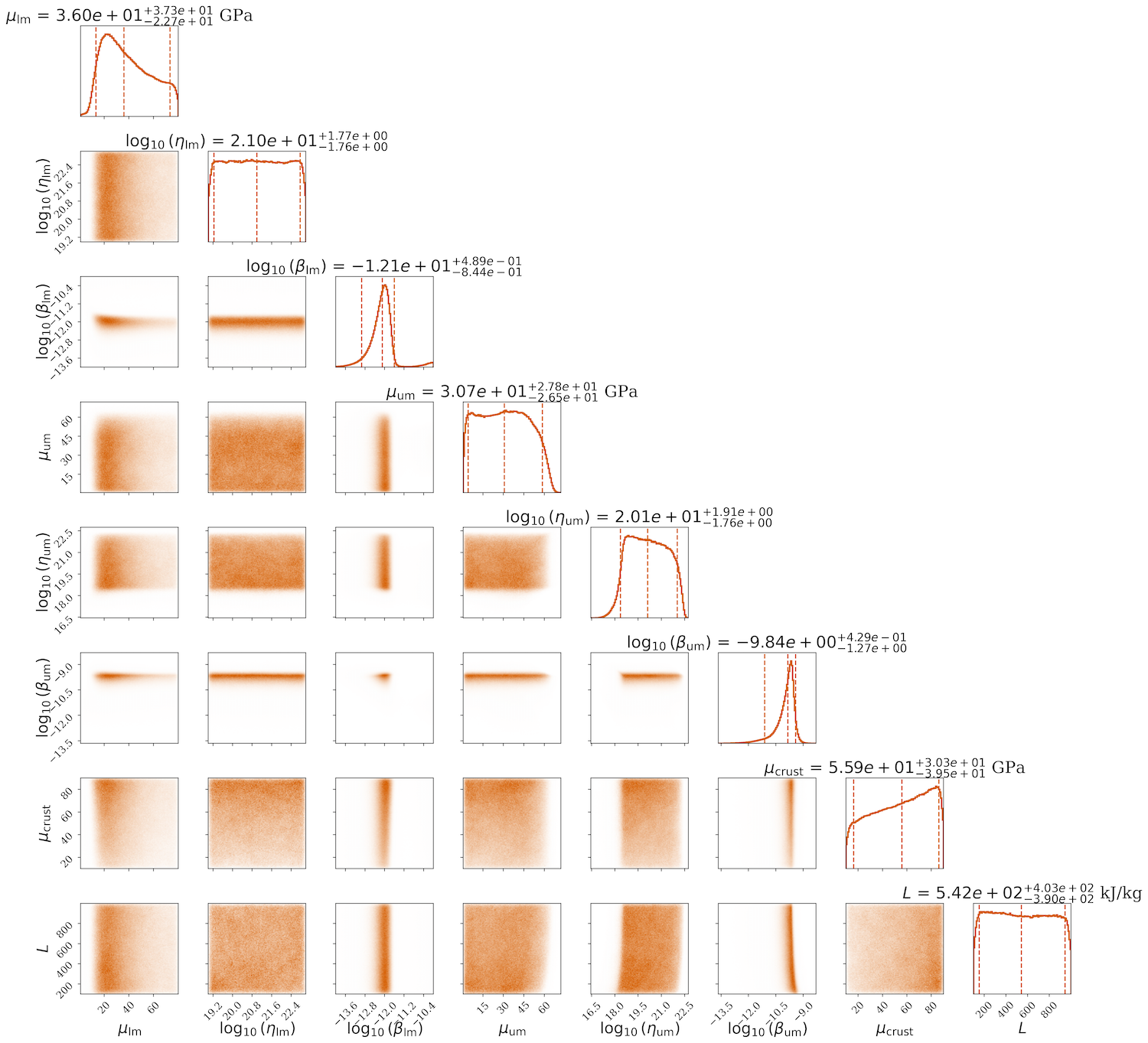
Methodology: Interior models are inverted using a Bayesian MCMC framework [6, 7]. To ensure robust parameter space sampling and mitigate initial condition dependence, we employ 15 independent chains, each yielding 250,000 accepted models. Following a 50,000-model burn-in period per chain, the converged samples are combined into a final posterior distribution of 3,000,000 models. Io is represented as a four-layer body comprising a fluid core, viscoelastic lower and upper mantle, and an elastic crust. Mantle rheology follows an Andrade formulation with a fixed frequency exponent α=0.3, while the compliance parameter β, layer thicknesses, and densities are treated as free variables. The specific latent heat of fusion (L) of the upper mantle is included as a free parameter to evaluate thermodynamic uncertainties in melt production. To account for deviations from hydrostatic equilibrium, non-hydrostatic gravity contributions (C20nh, C22nh) are introduced as free parameters [5]. Observed gravity coefficients are thus modeled as the sum of these non-hydrostatic terms and the hydrostatic components derived from internal interface shapes using a fourth-order formulation [8]. The complex degree-2 Love number k2 is computed via an adapted version of the PyALMA code [9], incorporating a self-consistent thermo-viscoelastic loop [10, 11]. For each sampled configuration, radial tidal dissipation profiles are coupled with magmatic transport equations [12]. Upper mantle rheological properties, such as viscosity, shear modulus, and the Andrade parameter β, are iteratively updated based on the local melt fraction Φ(r) until thermal and mechanical equilibrium is reached [10, 11]. This approach enables the determination of the maximum melt fraction (Φmax) within the upper mantle to assess the stability of a "magmatic sponge" configuration against the formation of a global magma ocean [13, 14, 15]. Longitudinal libration amplitude is computed for each accepted model to ensure consistency with no magma ocean models [5, 16].
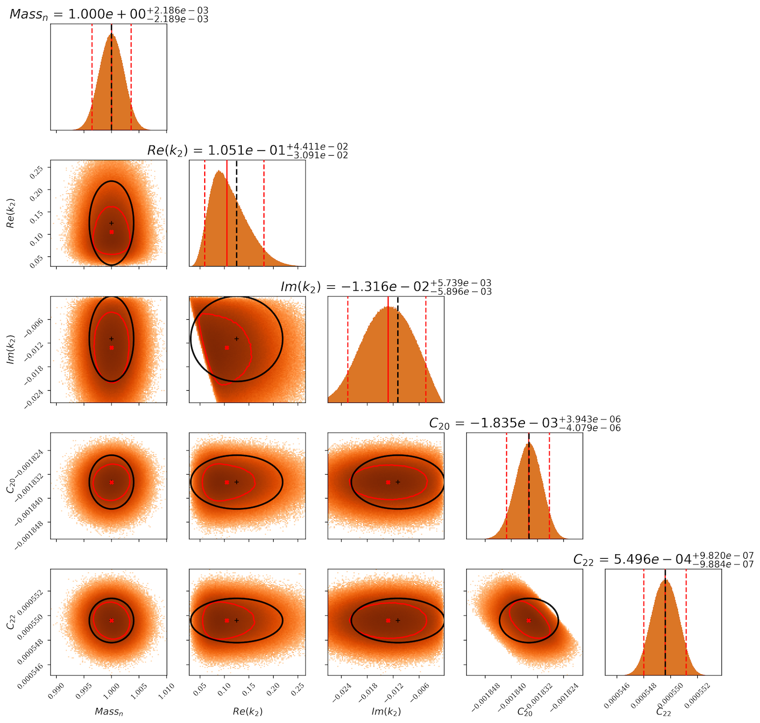
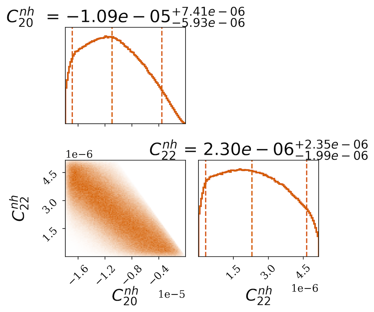
Inversion Results: Posterior distributions for layer thicknesses, densities, and mantle rheological properties are recovered through a comprehensive exploration of the parameter space (Figure 1). The accurate recovery of the target geophysical observables, including Io's mass, the static gravity harmonics, and both components of the complex Love number k2 (Figure 2), alongside the inversion of the non-hydrostatic gravity contributions (Figure 3), combined with thermodynamic equilibrium requirements, substantially reduces the range of admissible interior configurations.
The resulting posterior distribution of Φmax is characterized by a median value of 0.080; the upper bound of the 95.5% credible interval remains below the rheologically critical threshold of 0.20 [13], demonstrating that partial melt is structurally retained within a solid rock matrix rather than coalescing into a uniform liquid layer. These findings provide strong evidence against the existence of a global, fully liquid magma ocean, supporting instead a stable "magmatic sponge" configuration [13, 15]. The accepted models yield a predicted longitudinal libration amplitude of 263.9-19.4+18.9 m. This result is consistent with independent estimates reported in the literature [5, 16].
This methodology establishes a framework for rigorously constraining Io’s interior dynamics through the joint inversion of Juno gravity and complex k2 within a fully self-consistent thermo-viscoelastic–melt coupling.

Figure 1: MCMC posterior distributions for the retrieved rheological and structural parameters. The panels illustrate the probability densities for shear moduli, viscosities, and Andrade compliance parameters (β) for the crust and mantle layers, alongside the specific latent heat of fusion (L) for the upper mantle.

Figure 2: MCMC posterior distributions for the target geophysical observables: Io's mass, the static gravitational harmonic coefficients C20 and C22, and the real and imaginary components of the complex degree-2 Love number k2 [4,5]. Observational constraints are shown in black with their 1-σ uncertainties. The 2D marginal distributions are displayed as contour levels corresponding to the 16th and 84th percentiles (red).

Figure 3: MCMC posterior distributions for the non-hydrostatic gravitational harmonic coefficients C20nh and C22nh.
Acknowledgments: We thank Agenzia Spaziale Italiana (ASI) for the support of the JIRAM contribution to the Juno mission; this work is supported by the ASI–INAF Addendum n. 2016-23-H.3-2023 to grant 2016-23 H.0. AG acknowledges funding from the Italian Space Agency (ASI) grant n. 2023-60-HH.0.
References:
[1] Veeder, G. J. et al. (1994) J. Geophys. Res., 99(E8), 17095-17162.
[2] Peale, S. J. et al. (1979) Science, 203(4383), 892-894.
[3] Keane, J. T. et al. (2021) BAAS, 53, 178.
[4] Lopes, R. M. C. et al. (2023) Io: A New View of Jupiter’s Moon, Springer.
[5] Park, R. S. et al. (2025) Nature, 638, 69–73.
[6] Genova, A. et al. (2019) Geophys. Res. Lett., 46, 3625–3633.
[7] Petricca, F. et al. (2023) Geophys. Res. Lett., 50, e2023GL104016.
[8] Tricarico, P. (2014) Astrophys. J., 782, 99.
[9] Petricca, F. et al. (2024) Icarus, 417, 116120.
[10] Bierson, C. J. & Nimmo, F. (2016) J. Geophys. Res., 121, 2211–2224.
[11] Paris, M. et al. (2026) arXiv e-prints, arXiv:2603.19095.
[12] Moore, W. B. (2001) Icarus, 154, 548–550.
[13] Miyazaki, Y. & Stevenson, D. J. (2022) Planet. Sci. J., 3, 256.
[14] Tyler, R. H. et al. (2015) Astrophys. J. Suppl. Ser., 218, 22.
[15] Mura, A., et al. (2026). J. Geophys. Res., 131, e2025JE009047
[16] Van Hoolst, T. et al. (2020) J. Geophys. Res., 125, e2020JE006473.
How to cite: Paris, M., Mura, A., Genova, A., Zambon, F., Tosi, F., Gargiulo, A. M., Ciambellini, M., Boccacci, G., Bolton, S., Cicchetti, A., Noschese, R., Piccioni, G., Plainaki, C., Sindoni, G., and Sordini, R.: Bayesian inversion of Io's interior: self-consistent rheology from Juno gravity data and tidal dissipation, Europlanet Science Congress 2026, The Hague, The Netherlands, 7–11 Sep 2026, EPSC2026-287, https://doi.org/10.5194/epsc2026-287, 2026.
The surfaces of several outer Solar System moons display activity that cannot result from radiogenic and primordial heat alone, indicating that tidal heating drives their interior evolution. Tidal heating is the result of orbital eccentricities sustained over geological timescales by mean-motion resonances between moons [1], coupling interior and orbital evolution. Such resonances are common in the Solar System, and potentially also in compact exoplanetary systems: they drive sustained volcanism on Io [2] and maintain subsurface oceans on Europa and Enceladus today [3]. Understanding moons in the Solar System and beyond therefore requires a comprehensive picture of their coupled interior-orbital evolution.
In the past, tools used to study the interior-orbital evolution have typically been closed-source, limited to a specific body or set of assumptions or difficult to start working with. This raises the barrier-to-entry for researchers without the prerequisite background and makes reproducing results difficult. To solve these problems, we are developing DelfTIDE (Delft Tidal, Interior and Dynamical Evolution toolkit), an open-source, accessible and flexible framework for coupled interior-orbital modelling in multibody systems.
DelfTIDE represents the bodies in a system modularly: the model describing a body is separated into an interior, orbital and tidal model. We provide default implementations for each, based on common models in literature but users can also provide their own.
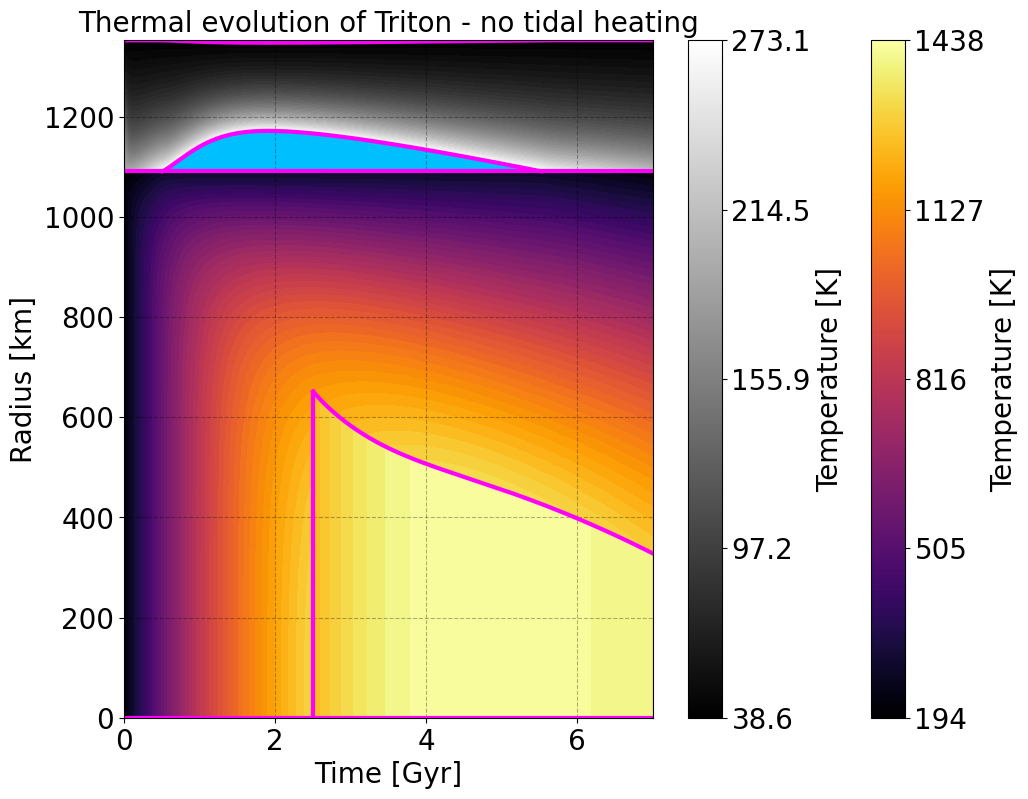
Regarding interior evolution, DelfTIDE’s layered interior models enable the user to flexibly model layered, spherically symmetric bodies. Currently implemented layers include conduction (time-dependent and equilibrium profiles), parametrised convection, and ocean layers. Application of boundary conditions, transitions between heat transport mechanisms (e.g., ocean formation or convection onset) and mass conservation are handled automatically by the code (e.g., Fig. 1).
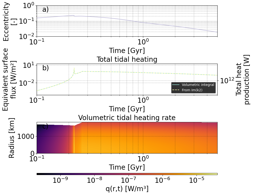
Tidal heating and its radial distribution are computed self-consistently with the interior model using the matrix propagator approach [4, 5, 6]. Orbital evolution can be evaluated for isolated moons or those in simple two-moon resonances using averaged equations of motion ( e.g., Fig. 2) [7], or in resonances analogous to the Laplace resonance [8].
To open the tool for use by non-experts and students, DelfTIDE puts special emphasis on accessibility. For instance, it includes a web-based GUI that allows one to compute the tidal response of planetary objects. We also provide the user with an LLM interface tailored to our codebase, enabling them to quickly set up simulations of new bodies and systems, or ask questions about the code.

Figure 1: Interior evolution for Triton accounting only for CI-chondrite radiogenic heating (from [9]), and no tidal heating. Boundaries between various layers are marked by the magenta lines: from top to bottom, these are the convective part of the mantle (when present), the conductive part of the mantle, the ocean (when present), and the icy shell.

Figure 2: Eccentricity (a), and total (b) and volumetric (c) tidal heating rate for an Io-like moon in a 2:1 resonance. The interior is comprised of a conductive lithosphere atop a convective mantle: dissipation is limited to the convective region. Feedback between interior and orbital evolution establishes an equilibrium tidal heating rate and corresponding eccentricity.

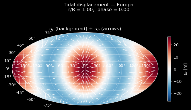
Figure 3: Surface deformation in the radial (background) and tangential (arrows) directions for a Europa-like moon, computed using DelfTIDE’s tidal module. The interior is comprised of a liquid core, silicate mantle, liquid ocean and a convective icy shell with a conductive lid, with representative homogeneous mechanical properties. Tidal forcing is applied at Europa’s orbital frequency.
[1] Murray, C. D., & Dermott, S. F. (1999). Solar System Dynamics. Cambridge University Press.
[2] Peale, S. J., Cassen, P., & Reynolds, R. T. (1979). Melting of Io by tidal dissipation. Science, 203(4383), 892–894. https://doi.org/10.1126/science.203.4383.892
[3] Nimmo, F., & Pappalardo, R. T. (2016). Ocean worlds in the outer solar system. Journal of Geophysical Research: Planets, 121(8), 1378–1399. https://doi.org/10.1002/2016JE005081
[4] Sabadini, R., Vermeersen, B., & Cambiotti, G. (2016). Global Dynamics of the Earth (Second). Springer Nature.
[5] Tobie, G., Mocquet, A., & Sotin, C. (2005). Tidal dissipation within large icy satellites: Applications to Europa and Titan. Icarus, 177(2), 534–549. https://doi.org/10.1016/j.icarus.2005.04.006
[6] Beuthe, M. (2013). Spatial patterns of tidal heating. Icarus, 223(1), 308–329. https://doi.org/10.1016/j.icarus.2012.11.020
[7] Dermott, S. F., Malhotra, R., & Murray, C. D. (1988). Dynamics of the Uranian and Saturnian Satellite Systems: A Chaotic Route to Melting Miranda? Icarus, 76, 295–334.
[8] Hussmann, H., & Spohn, T. (2004). Thermal-orbital evolution of Io and Europa. Icarus, 171(2), 391–410. https://doi.org/10.1016/j.icarus.2004.05.020
[9] Hussmann, H., Choblet, G., Lainey, V., Matson, D. L., Sotin, C., Tobie, G., & van Hoolst, T. (2010). Implications of rotation, orbital states, energy sources, and heat transport for internal processes in icy satellites. Space Science Reviews, 153(1–4), 317–348. https://doi.org/10.1007/s11214-010-9636-0
How to cite: van Woerkom, Q., Rovira-Navarro, M., Fayolle, S., Veenstra, A., and van der Wal, W.: Accessible modelling of coupled orbital-interior evolution using DelfTIDE, Europlanet Science Congress 2026, The Hague, The Netherlands, 7–11 Sep 2026, EPSC2026-601, https://doi.org/10.5194/epsc2026-601, 2026.


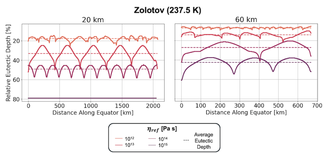
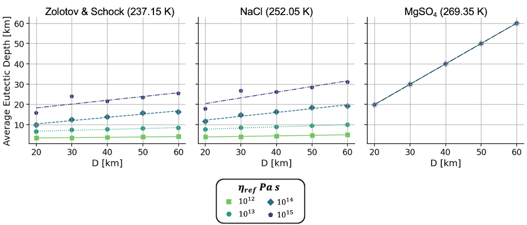
How to cite: Byrne, W., Plesa, A.-C., Postberg, F., Hussman, H., Schroeder, D., Steinbrügge, G., Wolfenbarger, N., and Cascioli, G.: Constraining Geophysical Properties of Europa’s Ice Shell from the Depth to Eutectic Interfaces, Europlanet Science Congress 2026, The Hague, The Netherlands, 7–11 Sep 2026, EPSC2026-185, https://doi.org/10.5194/epsc2026-185, 2026.
Enceladus, Saturn’s sixth-largest moon, is encased in a crust of nearly pure water ice that makes it one of the most reflective bodies in the Solar System (Howett et al., 2010). This "fresh-material"-like appearance is due to the continuous fallout of icy grains from the moon’s massive south polar plume (Postberg et al., 2011), which recoats the surface in a bright, porous regolith.
Enceladus is arguably the most geophysically active moon in the Solar System, presenting a high-priority target for the next generation of planetary exploration. Recognizing its immense astrobiological potential, the European Space Agency (ESA) has identified an Enceladus orbiter and lander as the primary candidate for its L4 flagship mission within the Voyage 2050 framework.
Current data suggest a surface dominated by a continuous fallout of plume-derived ice grains, ranging from sub-micron to tens of micrometers in diameter (Jaumann et al., 2008; Postberg et al., 2011; Scipioni et al., 2017; Morello & Berg, 2024). While the moon’s south polar plumes provide a direct window into its subsurface ocean (Postberg et al., 2009), the physical state and observable signatures of the resulting surface regolith remain difficult to directly probe and therefore poorly constrained.
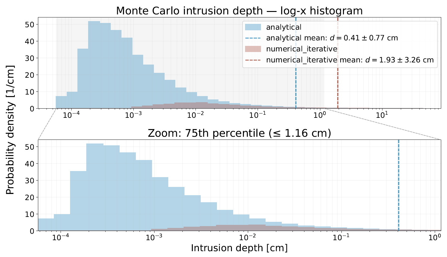
Fortunately, experiments have provided the first insights into the compressional behavior (compression curve: Φ(p); here Φ is the volume filling factor and p the applied pressure) of micrometer-sized water ice particles at low temperatures (Lorek et al., 2016; Kreuzig et al., 2023), which can be translated into a lander intrusion depth. Based on the recent work by Blum et al. (2026), the laboratory findings and the very low gravity of the icy moon, we developed a model to predict the intrusion depth of a potential lander. Initial results indicate intrusion depths in the mm to cm range as presented in Fig. 1, while further details regarding the model will be presented at the conference.

Fig. 1: Monte Carlo analysis showing a nominal intrusion depth of 0.4 cm (analytical mean), and 1.9 cm (numerical iterative mean).
References:
Howett et al. (2010) – DOI: 10.1016/j.icarus.2009.07.016
Postberg et al. (2011) – DOI: 10.1038/nature10175
Jaumann et al. (2008) – DOI: 10.1016/j.icarus.2007.09.013
Scipioni et al. (2017) – DOI: 10.1016/j.icarus.2017.02.012
Brown et al. (2006) – DOI: 10.1126/science.1121031
Gundlach et al. (2018) – DOI: 10.1093/mnras/sty1839
Morello & Berg (2024) – DOI: 10.1016/j.jqsrt.2024.109018
Lorek et al. (2016) – DOI: 10.1051/0004-6361/201526565
Kreuzig et al. (2023) – DOI: 10.1093/rasti/rzad049
Blum et al. (2026) – DOI: 10.1051/0004-6361/202558471
How to cite: Gundlach, B., Aussel, B., Rückriemen-Bez, T., Güttler, C., Ligterink, N., Cazaux, S., Hagermann, A., and Blum, J.: Enceladus surface: modeling intrusion depth for future lander missions, Europlanet Science Congress 2026, The Hague, The Netherlands, 7–11 Sep 2026, EPSC2026-885, https://doi.org/10.5194/epsc2026-885, 2026.
Please decide on your access
Please use the buttons below to download the supplementary material or to visit the external website where the presentation is linked. Regarding the external link, please note that Copernicus Meetings cannot accept any liability for the content and the website you will visit.
Forward to presentation link
You are going to open an external link to the presentation as indicated by the authors. Copernicus Meetings cannot accept any liability for the content and the website you will visit.
We are sorry, but presentations are only available for conference attendees. Please register for the conference first. Thank you.
Dwarf planet Ceres is the largest asteroid-belt body and may have sustained a global ocean for hundreds of millions to perhaps billions of years. Some thermal models suggest that a deep brine-rich layer may still be possible beneath its surface today [1].
Occator (approx. 92 km diameter) is a crater on Ceres' surface and is unique for its “bright spots”, known as the Cerealia and Vinalia Faculae. These bright spots are geologically young, high-albedo (7x background Ceres) salt deposits probably formed by some mechanism of brine mobilisation [2,3,4], making them an ideal window into Ceres' interior and its past or present brines. Infrared spectroscopy has shown that the composition of the faculae includes sodium carbonates and ammonium chlorides consistent with an ascent from the deep brine layer [5,6], but not all salts are as readily detectable at infrared wavelengths. In particular, halite (anhydrous NaCl) is featureless in the infrared in its pure form, but develops characteristic absorption features at visible wavelengths (0.46 µm and 0.72 µm) from lattice impurities (called “colour centers”) when exposed to radiation [7,8]. One study found potential spectral evidence for these colour centers in Dawn VIR data at Cerealia Facula, Ahuna Mons, and several impact craters, but the visible channel of the VIR instrument suffered from significant calibration uncertainties, and clear colour-center absorptions remain ambiguous across published reductions [9].
We will present new visible-wavelength spectra of the Occator crater region on Ceres obtained with the STIS instrument on the Hubble Space Telescope (HST). We compare our spectra to Dawn observations and past global-scale HST observations and analyse our spectra for halite colour centers, placing constraints on the presence of halite within Occator crater and thus the chemistry of the faculae.
[1] Castillo-Rogez, J. C., Hesse, M. A., Formisano, M., et al. 2019, Geophysical Research Letters, 46, 1963, doi: 10.1029/2018GL081473
[2] Stein, N. T., Ehlmann, B. L., Palomba, E., et al. 2019, Icarus, 320, 188, doi: 10.1016/j.icarus.2017.10.014
[3] Nathues, A., Schmedemann, N., Thangjam, G., et al. 2020, Nature Astronomy, 4, 794, doi: 10.1038/s41550-020-1146-8
[4] Scully, J. E. C., Bowling, T., Bu, C., et al. 2020, Nature Communications, 11, 3680, doi: 10.1038/s41467-020-15973-8
[5] De Sanctis, M. C., Raponi, A., Ammannito, E., et al. 2015b, Nature, 536, 54, doi: 10.1038/nature18290
[6] Raponi, A., De Sanctis, M. C., Carrozzo, F. G., et al. 2019, Icarus, 320, 83, doi: 10.1016/j.icarus.2018.02.001
[7] Hand, K. P., & Carlson, R. W. 2015, Geophysical Research Letters, 42, 3174–3178. doi: 10.1002/2015GL063559
[8] Trumbo, S. K., Brown, M. E., & Hand, K. P. 2019, Science Advances, 5, eaaw7123, doi: 10.1126/sciadv.aaw7123
[9] Bramble, M. S., & Hand, K. P. 2022, Geophysical Research Letters, 49, e2021GL096973, doi: 10.1029/2021GL096973
How to cite: Hekster, A. and Trumbo, S.: HST Search for Irradiated NaCl on the Surface of Ceres, Europlanet Science Congress 2026, The Hague, The Netherlands, 7–11 Sep 2026, EPSC2026-735, https://doi.org/10.5194/epsc2026-735, 2026.
The four Galilean moons of Jupiter have different surface characteristics. There are many reasons that may cause the difference. One of the most important factors is the tidal force from Jupiter, which could generate different tidal heat inside the moons. In order to demonstrate this point, we establish elastic mechanics equation to calculate the displacement in satellites’ interior. We obtain the tidal energy dissipation and surface heat flux of Galilean moons. We also find that the tidal response of Galilean moons is related to physical parameters including the distance from Jupiter, the diameter, the density, the orbital period, which may explain different energy dissipation in their interior.
How to cite: Chen, C. and Ma, X.: Different Surface Characteristics of Galilean Moons Caused by Tidal Forces from Jupiter, Europlanet Science Congress 2026, The Hague, The Netherlands, 7–11 Sep 2026, EPSC2026-24, https://doi.org/10.5194/epsc2026-24, 2026.
The Jovian moons Ganymede and Europa are prime targets for the exploration of icy moons by ESA’s JUICE and NASA’s Europa Clipper missions [1,2]. Future measurements from these missions will provide key insights into the structure of their ice shells and the depth of their subsurface oceans. Although the ocean represents the largest water reservoir beneath the surface, localized liquid brine reservoirs may also exist within the shallow subsurface of the ice shell. These reservoirs could serve as niches for habitability and provide ideal targets for exploration due to their proximity to the surface (∼1-5 km depth [e.g., 3]). The ice-penetrating radars REASON and RIME; onboard Europa Clipper and JUICE, respectively, will provide critical measurements to complement data from cameras (JANUS - JUICE; EIS - Europa Clipper), spectrometers (MAJIS - JUICE), and the in-situ dust analyzer SUDA (Europa Clipper), to provide a comprehensive picture of potential shallow habitats.
One of the top priorities of the two missions is the characterization of conditions that may have led to the emergence of habitable environments among the Jovian icy satellites through the investigation of past and/or recent geologic activity and its connection to the shallow subsurface, along with potential interactions with a subsurface ocean. Signs of possible past geologic activity were already observed in a few isolated spots on Ganymede's surface during the Voyager and Galileo missions. These spots have been described as "scalloped depressions" or "paterae" and have been interpreted as potential source vents for cryovolcanism, resembling possible calderas [e.g., 4,5]. An alternative origin related to diapirism has been proposed as well [6].
Most of the paterae have not been observed by imaging instruments with sufficient spatial resolution, and complementary information on local topography, surface age, and composition has not yet been acquired, preventing the discovery of unequivocal evidence for their origin, any potential interaction with Ganymede's subsurface ocean, and their relationships to the satellite's habitability [5]. Future measurements by JUICE will provide important information on the origin, overall characteristics, and formation mechanisms of Ganymede’s paterae.
In the case of relatively young paterae, possible associated liquid pockets in the shallow subsurface could provide clear evidence of processes related to the interaction with Ganymede's subsurface ocean. Reports of possible shallow liquid pockets in the ice shell have been extensively proposed for Europa as well [e.g., 3,7]. In particular, a recent study performed detailed geomorphological-structural investigations of Ménec Fossae, located within the major band Libya Linea [8]. The observed tectonic activity in this region of Europa could be related to a shallow water pocket located close to the surface, which would explain the observed overall topography of this area, in addition to the presence of specific geological features such as chaos terrain and double ridges. Comparing the observations on the two icy moons is therefore critically important, as analogies in their morphology, topography, and tectonic/fracture patterns could indicate similar processes at depth, either ongoing or relict.
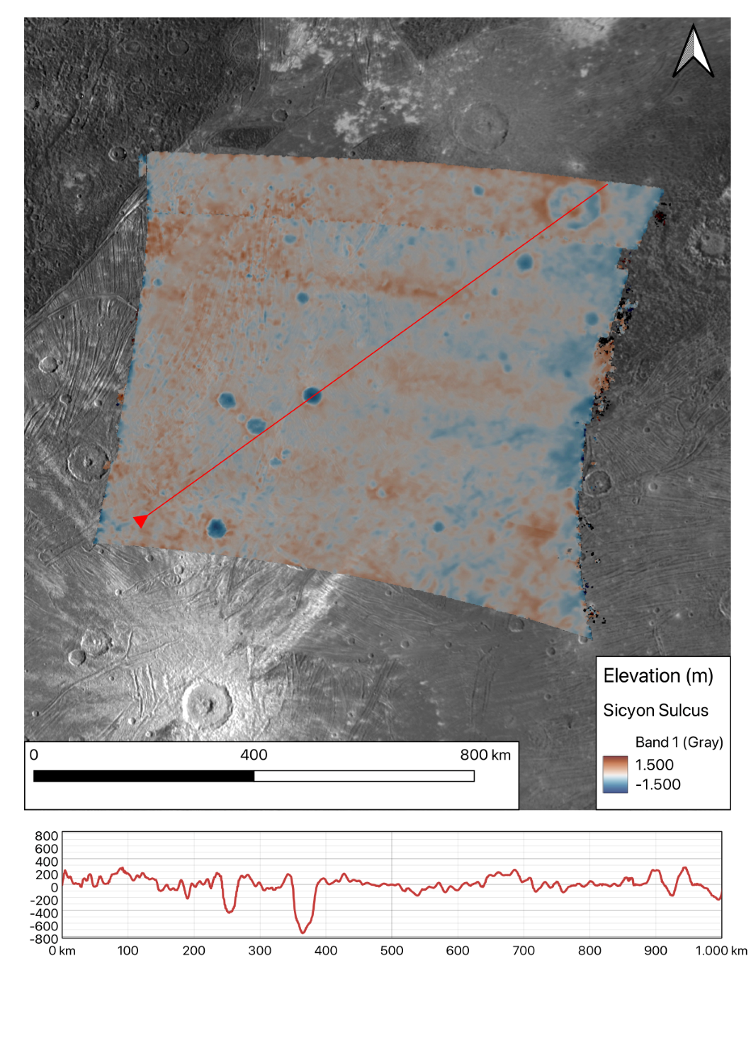
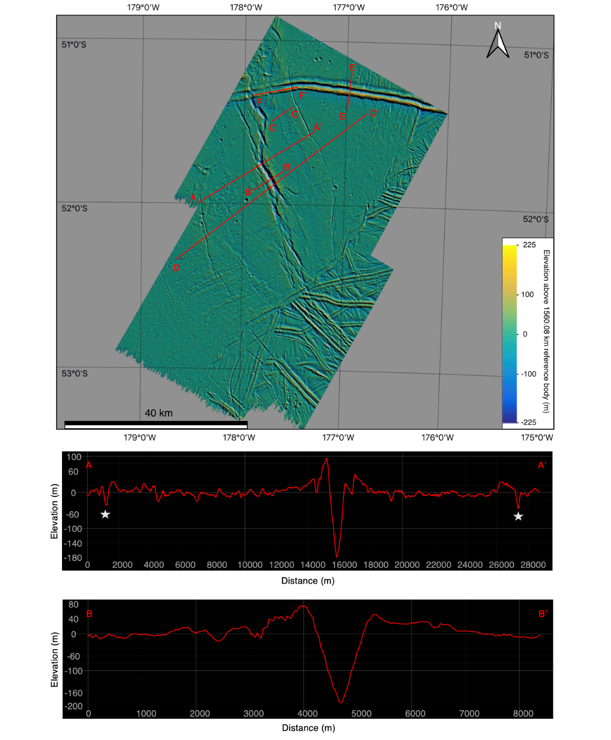
In this work, we conduct geomorphological and topographic analyses of surface features on both Ganymede and Europa, potentially related to shallow water bodies located within their ice shells. We aim to obtain a comprehensive view, constrained by the resolution of currently available data, of such young and/or relict features, likely representing some of the most astrobiologically relevant locations on both Ganymede and Europa. Here, we specifically focus on Digital Terrain Model (DTM) production and analysis, based on JUNO stereo pairs in the case of Ganymede (Figure 1) and on shape-from-shading techniques for Europa (Figure 2). This work will inform the planning of future stereo observations of paterae on Ganymede by the JANUS camera onboard JUICE [9], to better understand the moon’s habitability potential.

Figure 1. Digital Terrain Model (DTM) example for Ganymede, based on stereo coupling of JUNO images JNCR_2021158_34C00001_V01 and JNCR_2021158_34C00002_V01. Legend shows the elevation values, comprised between -1500 and 1500 m in relation to Ganymede’s reference ellipsoid.

Figure 2. Shape-from-shading digital terrain model (DTM) of Ménec Fossae on Europa, individual DTMs are of 9926r and 9939r Galileo Solid-State Imager (SSI) image frames, later mosaicked together. From [8].
References:
[1] Grasset et al. (2013), PSS. https://doi.org/10.1016/j.pss.2012.12.002
[2] Pappalardo et al. (2024), SSR. https://doi.org/10.1007/s11214-024-01070-5
[3] Chivers et al. (2021), JGR: Planets. https://doi. org/10.1029/2020JE006692
[4] Schenk et al. (2001), Nature. https://doi.org/10.1038/35065027
[5] Stephan et al. (2021), PSS. https://doi.org/10.1016/j.pss.2021.105324
[6] Giese et al. (2017), 48th LPSC Abstracts. No. 1964 p. 2474
[7] Craft et al. (2016), Icarus. https://doi.org/10.1016/j.icarus.2016.01.023
[8] Matteoni et al. (2023), JGR: Planets. https://doi.org/10.1029/2022JE007623
[9] Palumbo et al. (2025), SSR. https://doi.org/10.1007/s11214-025-01158-6
How to cite: Matteoni, P., Walter, S., Aye, K.-M., Lamers, G., Hauber, E., Stephan, K., and Postberg, F.: Geomorphological and Topographic Analysis of Shallow Subsurface Water Reservoirs on Ganymede and Europa, Europlanet Science Congress 2026, The Hague, The Netherlands, 7–11 Sep 2026, EPSC2026-1022, https://doi.org/10.5194/epsc2026-1022, 2026.
Introduction
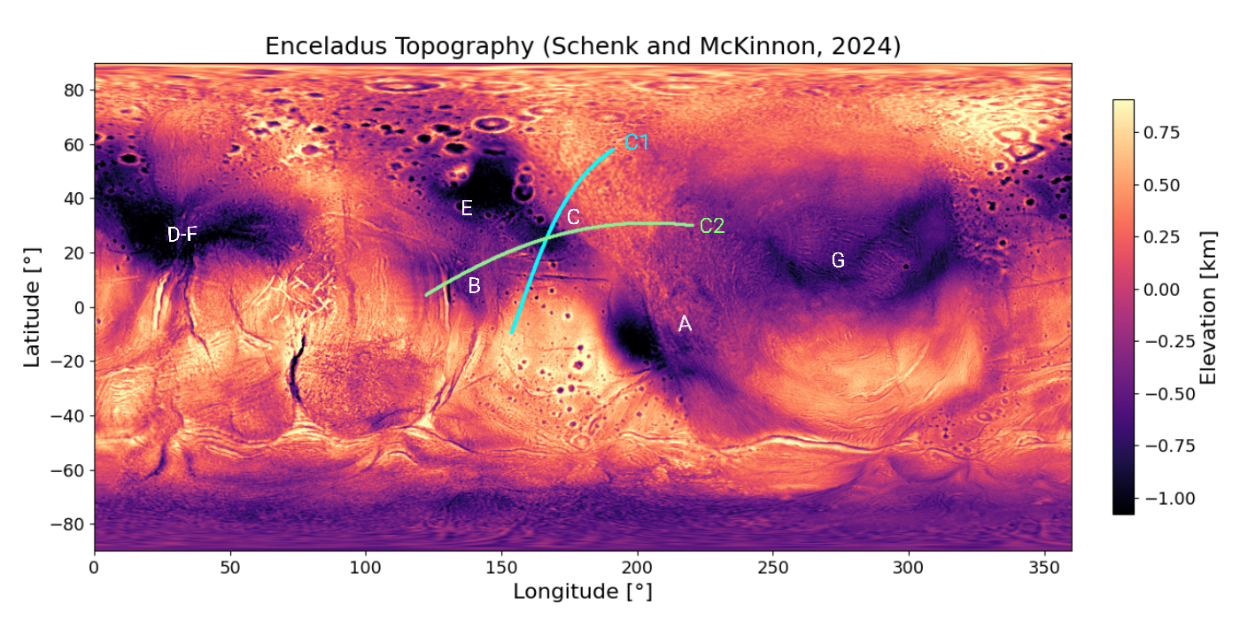
Icy moons are a primary focus of the planetary science community due to their potentially habitable subsurface oceans. Enceladus is particularly intriguing because of its anomalous thermal activity, driven by tidal dissipation in its porous silicate core [1]. While the most prominent features are the 'Tiger Stripes'—fractures on the south polar terrain through which massive cryovolcanic plumes erupt—other notable features have recently been highlighted [2–4]. These include large, 100-km-scale depressions of unknown origin approximately 1–1.5 km deep, which appear too smooth to be tectonic or impact-related (Figure 1, A–G). In our study, we focused mainly on basin C and its topography along the great circles C1 and C2 (blue and green lines in Figure 1).

Figure 1: Enceladus’ topography. The regional depressions identified in [4] are labelled A–G. The topography predicted in this study is compared with the observation for depression C (blue and green lines C1 and C2).
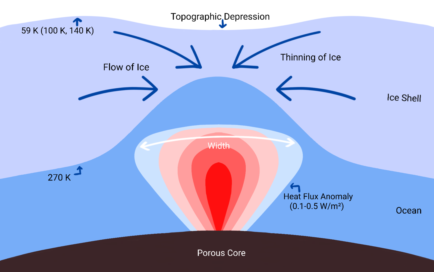
As suggested by Schenk and McKinnon [4], these features may be a manifestation of hydrothermal vents originating in the porous core. According to this hypothesis, the regional depression forms as a viscous response to the heat flux anomaly coming from the ocean. Thinning of the ice shell causes a flow of ice to the area above the heat flux anomaly, which results in a topographic depression at the surface (Figure 2). Here we test this hypothesis using a numerical model, conduct a parametric study, and compare our modeling results with the topography observed during the Cassini mission.
Method
To investigate the scenario described above, we have developed a numerical code that solves the viscous deformation of the ice shell in spherical axisymmetric geometry using the finite element software FEniCS [5]. We solve the equations of mass, momentum, and energy conservation, employing free-surface boundary conditions at both the surface and the ice-ocean interface, where we also account for the ice-water phase transition. To evolve the shape of the boundaries, we use the ALE method [6]. The model accounts for the temperature dependence of ice viscosity. We assume a basal temperature of 270 K and vary the surface temperature (59 K, 100 K, and 140 K) to mimic the insulating effect of a regolith layer [7]. The hydrothermal activity is represented by a Gaussian heat flux anomaly at the ice-ocean interface, with amplitudes ranging from 0.1 to 0.5 W/m2 and a width of 60 km.

Figure 2: Illustration of the modeled scenario. The heat flux coming from the ocean results in melting the ice, driving the viscous flow in the ice shell, and leading to the formation of a regional depression.
Results
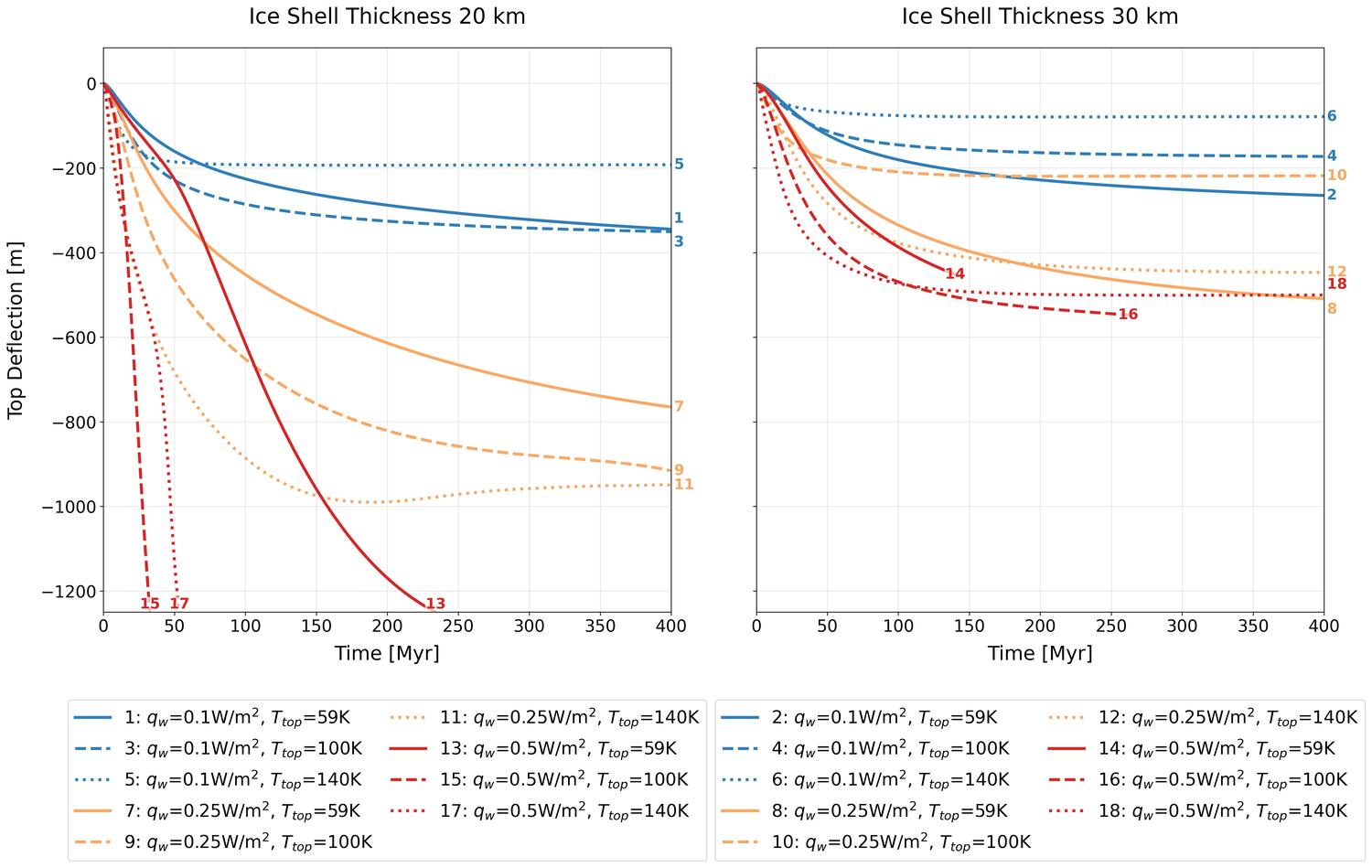
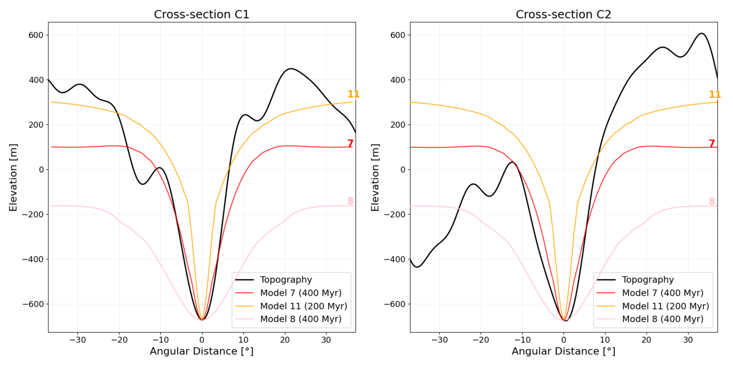
Figure 3 shows the evolution of the depth of the surface depression for different model parameters. The characteristic times of the evolution strongly depend on the amplitude of the heat flux anomaly, ranging from a few tens of Myr for qw=0.5 W/m2 to hundreds of Myr for qw=0.1 W/m2. The rate of the convergence and the depth of the predicted depression are influenced by the average thickness of the ice shell, being significantly larger for a thin ice shell (Figure 3, left). In Figure 4, we compare some of our models with the topography observed by Schenk and McKinnon [4]. The best fit is achieved for the heat flux anomaly with the amplitude of 0.25 W/m2, the 20 km thick ice shell, and the surface temperature of 59 K. Note that simulations performed for a thicker ice shell produce wider topographical depressions (see, e.g., simulation 8 in the right panel of Figure 4).

Figure 3: Depth of the surface depression as a function of time computed for 20-km (left) and 30-km (right) ice shells assuming different amplitudes of the ocean heat flux (qw) and different surface temperatures (Ttop).

Figure 4: Comparison of selected models with the observed topography of basin C along the great circles C1 (left) and C2 (right) indicated in Figure 1. The observed topography corresponds to spherical harmonic degrees 4–40.
Conclusions
Our numerical simulations demonstrate that the hydrothermal vents originating in the core are a plausible explanation for the formation of deep, smooth 100-km-scale depressions observed on Enceladus’ surface. The rate of formation of these depressions strongly depends on the thickness of the ice shell and the amplitude of the anomalous heat flux coming from the ocean. Given that the plume in the ocean may be rather unstable (except in the case where it is located near the pole [8]), it is likely that the depressions were formed relatively quickly (≈10–50 Myr) during a period of enhanced tidal dissipation. Another possible explanation is that the depressions were formed relatively slowly near the pole (≈50–500 Myr) and then relocated due to the rigid rotation of the ice shell [2].
Acknowledgments
This research is supported by the GAUK project No. 436326 and by the Czech Science Foundation through project No. 25-16801S.
References
1. Choblet et al. (2017), Nat. Astron., 1, 841–847.
2. Tajeddine et al. (2017), Icarus, 295, 46–60.
3. Park et al. (2024), J. Geophys. Res. Planets, 129, e2023JE008054.
4. Schenk and McKinnon (2024), Icarus, 408, 115827.
5. Logg et al. (2012), The FEniCS Book, Springer–Verlag.
6. Donea et al. (2004), Encyclopedia of Computational Mechanics, John Wiley & Sons, pp. 413-437.
7. Martin et al. (2023), Icarus, 392, 115369.
8. Bouffard et al. (2025), Nat. Astron., 9, 650-657.
How to cite: Šindlerová, K. A., Kihoulou, M., and Čadek, O.: Uncovering the mystery of deep depressions on Enceladus’ surface, Europlanet Science Congress 2026, The Hague, The Netherlands, 7–11 Sep 2026, EPSC2026-346, https://doi.org/10.5194/epsc2026-346, 2026.
Io’s widespread volcanic activity is driven by strong tidal heating within its interior [1]. The distribution of tidal heating within Io's interior is closely linked to the moon's thermal state and its evolution [2,3]. Yet, despite years of observations [4], where inside Io heat is being dissipated remains largely unknown. For example, it remains unclear whether an asthenosphere (a low-viscosity layer beneath the crust) exists [4].
Ground-based and space-borne observations provide a window into Io's interior. With the recent measurement of Io’s tidal Love number k2 [5], there are now four independent gravity observations: C20, C22, and both parts of k2 [5,6]. This makes Io, together with Titan [7], the outer solar system moon for which we have the most gravity observations. Furthermore, there is a large database of volcanic activity observations [e.g., 4], assumed to link more directly to Io's tidal heating pattern. In turn, the heating pattern is sensitive to Io’s interior radial rheology structure [2], complementing the tidal response observations. However, no comprehensive Bayesian inversion exists that incorporates both gravity and volcanic activity observations.
We investigate how combining all gravity observations and the observed volcanic heat flux constrains Io’s interior. As a measure of how Io’s heat output is distributed, we use the ratio of polar to equatorial heat flux. Our interior model consists of four layers: core, mantle, asthenosphere, and lithosphere, and we compute the tidal response using Andrade rheology [8]. We use a Markov Chain Monte Carlo approach to integrate all gravity observations and the observed heat flux ratio to constrain Io’s interior.
Different observables are sensitive to different interior parameters. The static gravity coefficients, C20 and C22, constrain the core density and radius, k2-measurements the effective rigidity and viscosity, and the heat flux ratio the radial viscosity profile. The latter requires the majority of the heating (>90%) to occur in a low viscosity asthenosphere (1013 Pa s), even with conservative assumptions on the distribution of Io’s unmeasured background heat flux.
We thus show that, within current observational limits, Io must have an asthenosphere where a significant amount of its heat is generated. The existence of an asthenosphere is in line with previous results [9] and also expected from melt advection models [e.g., 10]. While we used Andrade rheology, we find viscosities that imply melt fractions at the edge of what is considered solid [e.g., 11], raising questions about the validity of rheology models typically used to model tidal deformation in planetary objects. However, experimental work on anelastic deformation under Io-like conditions is likely needed to resolve this problem [8]. Finally, our study provides statistically consistent ranges for Io’s interior parameters, which could be used in future studies.

Figure 1. The posterior PDFs of the ratio between energy dissipation in the asthenosphere (Ea) and mantle (Em) (subplot a), the polar-to-equatorial heat flux ratio (subplot c), and the ratio between asthenosphere and mantle viscosity ηx (subplot f). The 2-dimensional PDFs, indicating the correlations between two parameters, are given in the off-diagonal subplots. The three cases, without the observed polar flux ratio as one of the observables (blue), with the observed ratio (red), and with a uniform flux ratio (green), are plotted on top of each other. The dotted lines in the histograms and the contours in the 2D PDFs contain 68.3% of the cases.
References
[1] Peale, S. J., Cassen, P., & Reynolds, R. T. 1979, Science, 203, 892
[2] Segatz, M., Spohn, T., Ross, M. N., & Schubert, G. 1988, Icarus, 75, 187
[3] Hussmann, H. & Spohn, T. 2004, Icarus, 171, 391
[4] Davies, A. G., Perry, J. E., Williams, D. A., Veeder, G. J., & Nelson, D. M. 2024, The Planetary Science Journal, 5, 121
[5] Park, R. S., Jacobson, R. A., Gomez Casajus, L., et al. 2025, Nature, 638, 69
[6] Lainey, V., Arlot, J.-E., Karatekin, ¨O., & van Hoolst, T. 2009, Nature, 459, 957
[7] Petricca, F., Vance, S. D., Parisi, M., et al. 2025, Nature, 648, 556
[8] Bierson, C. J. 2024, Icarus, 414, 116026
[9] Bierson, C. J. & Nimmo, F. 2016, Journal of Geophysical Research (Planets), 121, 2211
[10] Spencer, D. C., Katz, R. F., Hewitt, I. J., May, D. A., & Keszthelyi, L. P. 2020, Journal of Geophysical Research (Planets), 125, e06604
[11] Scott, T. & Kohlstedt, D. L. 2006, Earth and Planetary Science Letters, 246, 177
How to cite: Veenstra, A., Rovira-Navarro, M., and van der Wal, W.: Inferring Io’s Internal Properties by Combining Gravity Measurements and Volcanic Activity, Europlanet Science Congress 2026, The Hague, The Netherlands, 7–11 Sep 2026, EPSC2026-309, https://doi.org/10.5194/epsc2026-309, 2026.
Introduction
Saturn’s moon Enceladus exhibits a unique pattern of surface deformation associated with ongoing geological activity driven by tidal forcing and internal processes. While features such as the south polar terrain and its eruptive fractures are striking manifestations of this activity, the underlying mechanisms are rooted in the global stress state of the ice shell.
This stress field arises from both external and internal sources. External forcing, induced by Saturn’s gravitational field acting on Enceladus, is represented by diurnal tides and any secular change of the tidal bulge, associated with non-synchronous rotation or any change in the orbital configuration. Internal sources are associated with ice flow driven by departures from hydrostatic equilibrium. Constraining how these processes generate and modulate the stress field is essential for understanding the moon’s mechanical behaviour and long-term evolution.
Model
We investigate the stress state within the viscoelastic ice shell across multiple spatial and temporal scales, with the mechanical response governed by the relationship between the forcing period and the viscous relaxation time. For forcing periods shorter than the relaxation time, deformation is predominantly elastic, allowing stresses to accumulate and potentially promote brittle failure. For longer forcing periods, inelastic deformation becomes increasingly pronounced in terms of viscoelastic Maxwell rheology. At the longest, geological time scales, purely viscous flow dominates.
To account for leading-order structural effects, we consider several models of shell thickness, in particular that of Čadek et al. (2019) derived from the shape model of Tajedinne et al. (2017), as well as recent shape models by Schenk et al. (2024) and Park et al. (2024). For diurnal tides, we also investigate the role of the presence or absence of faults in the south polar region, together with several parameterizations of their geometry, following Porco et al. (2014) and Rhoden et al. (2020). Faults are modelled either as narrow voids or as zones with a specific pseudo-plastic rheology, mimicking frictionless behaviour or Coulomb-type friction, respectively, following Pleiner Sládková et al. (2021).
On geological timescales, the ice shell is treated as a viscous fluid within the Boussinesq approximation, including gravitational effects from internal density variations and boundary topography, following Čadek et al. (2019). For the temperature and viscosity structure, we assume a simplified 1D conductive profile and an Arrhenius-type temperature dependence of viscosity. All numerical simulations are performed using the finite element method, following Alnæs et al. (2015), Souček et al. (2019), and Pleiner Sládková et al. (2021).
Results
We first analyse the instantaneous elastic response of the shell to tidal forcing over a single orbital period of 1.37 days. This response depends strongly on the shell shape and thickness, as well as on the geometry of the faults and their frictional parameterization. These factors control both the magnitude and orientation of the resulting stresses.
Viscoelastic effects associated with eccentricity-driven tides are relatively limited. They are mainly confined to a thin lowermost region near the ice-ocean interface, where the temperature reaches the melting point, and the viscosity decreases to approximately 1014 Pa s. As the forcing period increases, the contribution of the viscous component to the total response increases. Viscoelastic effects become dominant for slow non-synchronous rotation of the ice shell, particularly in the lowermost, low-viscosity regions. Here, we consider possible non-synchronous rotation periods ranging from 0.01 to 1 Myr, following Patthoff et al. (2019). Viscous weakening at the base of the ice shell effectively reduces its apparent elastic thickness; the induced stresses can reach up to several MPa. In this study, we compare different parameterizations of viscosity in terms of the viscosity value at the ice-ocean interface.
Finally, at geological timescales, we examine viscous flow driven by lateral variations in shell thickness for the aforementioned shell-thickness models. These variations generate density anomalies and associated gravitational imbalances, representing departures from hydrostatic equilibrium. The resulting flow redistributes mass toward a stable hydrostatic configuration, with velocities controlled by the viscosity contrast between the upper and lower shell boundaries. For realistic viscosity contrast across the shell, the flow is predominantly tangential along the ice-ocean interface. This flow pattern cannot be captured by simplified spectral methods that typically assume a shell of uniform thickness.


Conclusions
Our results show that Enceladus’ global stress state is controlled by the interplay between shell geometry, presence of faults and their properties, forcing timescale, and ice rheology. Using advanced three-dimensional finite element modelling, we quantify the relative effects of these processes across elastic, viscoelastic, and viscous deformation regimes.
Short-period tidal forcing produces a mainly elastic response, with stresses strongly affected by shell thickness variations and the mechanical behaviour of south polar faults. Viscoelastic effects are limited for diurnal tides but become important for longer-period forcing, particularly non-synchronous rotation, where basal weakening reduces the apparent elastic thickness of the shell and can generate stresses of several MPa.
On geological timescales, lateral shell-thickness variations drive viscous flow toward a more stable hydrostatic configuration. This flow is strongly influenced by the vertical viscosity contrast and may become localized along the ice-ocean interface, highlighting the need for fully three-dimensional models of Enceladus’ ice shell.
References
Alnaes, et al. (2015). doi: https://doi.org/10.11588/ans.2015.100.20553
Čadek et al. (2019), doi: https://doi.org/10.1016/j.icarus.2018.10.003
Patthoff et al. (2019), doi: https://doi.org/10.1016/j.icarus.2018.11.028
Schenk et al. (2024), doi: 10.1016/j.icarus.2023.115827
Park et al. (2024), doi: https://doi.org/10.1029/2023JE008054
Porco et al. (2014), doi: 10.1088/0004-6256/148/3/45
Rhoden et al. (2020), doi: https://doi.org/10.1016/j.epsl.2020.116389
Pleiner Sládková et al. (2021), doi: http://doi.org/10.1029/2021GL094849 .
Tajeddine et al. (2017), doi: https://doi.org/10.1016/j.icarus.2017.04.019
Souček et al. (2019), doi: https://doi.org/10.1016/j.icarus.2018.10.003
How to cite: Piláriková, B., Bakoč, A., Běhounková, M., Souček, O., Choblet, G., and Tobie, G.: Global stress state of Enceladus’ ice shell: effects of various deformation processes, Europlanet Science Congress 2026, The Hague, The Netherlands, 7–11 Sep 2026, EPSC2026-419, https://doi.org/10.5194/epsc2026-419, 2026.
As evidence for an interior salty, liquid water ocean on Jupiter’s moon Europa has grown over the last few decades, so too has the interest in modelling its interactions with the ice shell. Water is a key ingredient of life as we know it, and as such Europa has become a prime candidate in the search for habitable environments beyond Earth. Europa experiences significant tidal heating due to gravitational interactions with Jupiter during its orbit, which could sustain a subsurface liquid water ocean (Sotin et al., 2009). Measurements of an induced magnetic field from the Galileo mission (Kivelson et al., 2000) suggest that the ocean likely contains salts, which could help keep the ocean in a liquid state. Spectral signatures of salts have been detected in endogenic regions of Europa’s surface, pointing towards the further existence of salts within the ice shell itself, in the form of brine reservoirs (Trumbo et al., 2019). On Earth, certain organisms (halophiles) can survive and even thrive in such highly salty environments. As such, the presence of brines within Europa’s ice shell are of great interest in understanding its potential habitability (Wolfenbarger et al., 2022).
Subsurface brine reservoirs could form via melting caused by impacts or by the convective transport of liquid inclusions from the ice-ocean interface (which consists of a semi-liquid, mushy layer) to the near-surface of the ice shell (Buffo et al., 2020). The upcoming Europa Clipper and JUICE missions could probe the existence of such shallow subsurface brine reservoirs via radar sounding and gravity measurements (Pappalardo et al., 2024). Thus, this work not only endeavours to understand the large-scale evolution of such brine reservoirs but also informs such future missions on their detection.
In this study, we perform several solid-state, 2D geodynamical simulations using a 30 km ice shell thickness. In our models, we vary parameters such as ice grain size (values of 1cm, 1mm, and 0.1mm), salinity (concentrations of 1 x Earth ocean and 4 x Earth ocean salinity), surface ice yield stress (in a range of 15 kPa to 180 kPa), and spatial distribution of brines (Fig. 1). The goal is to determine how the variation of these parameters influences the transport and later distribution of the brines within the ice shell.

Figure 1: Non-dimensional density distribution for the four initial salt distribution scenarios.
The simulations are in a cylindrical geometry and are performed using the GAIA mantle convection code (Hüttig et al., 2013). GAIA is a finite-volume fluid flow solver that solves the conservation equations of mass, linear momentum, and thermal energy on a fixed computational grid. The advection and mixing of chemical components are modelled via a particle-in-cell approach, in which a transport equation is solved to move tracer particles carrying various chemical species according to the velocity field of the simulation. This method is essentially free of numerical diffusion and can treat the advection of an arbitrary number of different chemical components.
In our models, we test four distributions of salts through the ice shell: 1) a linear distribution, where, initially, the chemical density linearly decreases from the surface to the ice-ocean interface, 2) a step function, where the topmost 3 km (10%) of the ice shell are highly enriched in salts, 3) an exponential distribution, where the initial density profile decreases exponentially with depth, and 4) brine pockets, which consists of randomly generated brine pocket circles of radii between 250 and 2500 m and of varying salt concentrations. For the brine pockets distribution, we test two further scenarios, one where these brine pockets only exist in the upper half of the ice shell and another where they are distributed throughout the entire shell depth.
In our models we use a variable thermal conductivity and thermal expansivity, and include a pressure- and temperature-dependent composite Arrhenius viscosity that considers diffusion creep, dislocation creep, grain boundary sliding and basal slip. Furthermore, we investigate the effects of surface mobilisation on material transport and mixing. To this end, we employ a pseudo-plastic rheology where surface mobilisation occurs as soon as convective stresses exceed a predefined yield stress. We systematically decrease the yield stress until surface mobilisation takes place. This helps us determine the boundary between cases with surface mobilisation and surface material transport within the deeper ice shell, and cases that lie in a stagnant lid regime, a regime where an immobile layer forms at the top of the convective domain, due to the strong temperature-dependent viscosity. In the stagnant lid regime, the densest materials are trapped close to the surface and do not participate in the convection. In cases with surface mobilization, surface material can be brought into the deeper part of the ice shell, thereby facilitating surface-to-ocean exchange.
Our study will show how salts are redistributed over time throughout the ice shell under different initial conditions and will help guide future missions in the detection of such reservoirs. Further studies could build upon this work by varying the ice shell thickness and incorporating the effects of tidal heating.
References:
Sotin et al., Europa, (2009).
Trumbo et al., Science Advances 5, (2019).
Hüttig et al., PEPI 220, 11, (2013).
Kivelson et al., Science, 289, 1340-1343, (2000)
Wolfenbarger et al., Geophysical Research Letters, 49, (2022)
Buffo et al., Journal of Geophysical Research: Planets, 125, (2020)
Pappalardo et al., Space Science Reviews, 220:40, (2024)
How to cite: Lambert, G., Plesa, A.-C., and Hussmann, H.: Transport and mixing of salts in Europa’s ice shell: A geodynamic perspective, Europlanet Science Congress 2026, The Hague, The Netherlands, 7–11 Sep 2026, EPSC2026-844, https://doi.org/10.5194/epsc2026-844, 2026.
Jupiter’s moon Io, where tidal forcing is converted to extensive silicate volcanism, is an ideal setting for linking orbital stresses to heat generation through comparison with Earth volcanism and other tidally heated bodies. However, the total heat generated by tidal dissipation is contingent on the interior structure and distribution of melt, which influence temperature-dependent mechanical properties; this creates complex feedback loops involving tidal dissipation, melt generation and migration, lithospheric loading, and crustal stress states that facilitate magma ascent through deep faults (Keszthelyi et al., 2022).
The relationship between tidal heating and volcanism on Io therefore depends on the extent and depth of its partial melt, and thus its interior structure. While Io’s interior likely consists of an iron-rich core, silicate mantle, and crust (Breuer et al., 2022), the size of these layers and the likely regions of tidal heat generation are not well constrained. Previous studies suggest that Io’s most strongly heated, dissipative regions will be those containing a degree of partial melt, either through a shallow asthenosphere or in a deeper partially molten mantle (Keane et al., 2023). Given the uncertainty on melt depth and storage, it is difficult to model how Io’s surface magmatism relates to its interior processes, and therefore to fully understand the conversion between tidal stress and energy budgets.
Using the geodynamical code GAIA (Hüttig et al., 2013) to investigate the combined roles of melt depth and core size, we constructed two- and three-dimensional models of Io. GAIA is a finite-volume code that numerically solves the conservation equations of mass, linear momentum and thermal energy. Our models consider core cooling and radioactive decay as appropriate for a thermal evolution scenario, with tidal heating added per the Maxwell viscosity-dependent treatment of tidal heating by Tobie et al., 2003. Similar to Moore and Webb (2013), we consider fully extrusive cases in which the entire amount of melt produced in Io’s interior is extracted at the surface, followed by vertical downward-advection of cold surface material. Alternatively, we test the effect of magmatic intrusions created at depth, by emplacing only part of the melt produced in the interior at the surface, while the rest remains trapped in the lithosphere.
Our models were restricted to cases in which Io has a dominantly rocky interior with partial melt concentrations < 30%, in line with recent suggestions that Io lacks a present-day ocean (Park et al., 2025). The mantle viscosity in our models is temperature- and pressure-dependent and follows an Arrhenius law. We include the weakening effect of melt fraction on the viscosity through an additional exponential term that locally decreases the mantle viscosity when non-zero melt fractions are present. In our models, we vary the core size between 650 – 950 km, which we link to a core composition between a pure Fe and an Fe-FeS eutectic.
As already shown in previous studies (Moore & Webb, 2013; Lourenco et al., 2018; Herrera et al., 2026) melt extraction can play a major role for the thermal state of the lithosphere and affects partial melt production during the planetary history, with fully extrusive scenarios leading to thick and cold lithospheres, with deep melting zones. Highly intrusive models, however, are characterized by thin and warm lithospheres and shallow melt depths. The results of our simulations will show if and how the depth of partial melt storage within Io can be directly linked to surface heat flux, and the extent to which the predicted degree of melt depends on tidal heating parameters. Following these results, we will aim to predict tidal heating patterns that may be validated with future observational missions.
References
- Breuer, D., Hamilton, C.W., Khurana, K., 2022. The Internal Structure of Io. Elements 18, 385–390. https://doi.org/10.2138/gselements.18.6.385
- Herrera, C., Plesa, A.-C., Maia, J., Breuer, D., 2026. Surface temperature and mantle viscosity influence the cooling efficiency of magmatic styles on Venus (No. EGU26-1018). Presented at the EGU26, Copernicus Meetings. https://doi.org/10.5194/egusphere-egu26-1018
- Hüttig, C., Tosi, N., Moore, W.B., 2013. An improved formulation of the incompressible Navier–Stokes equations with variable viscosity. Physics of the Earth and Planetary Interiors 220, 11–18. https://doi.org/10.1016/j.pepi.2013.04.002
- Keane, J.T., Matsuyama, I., Bierson, C.J., Trinh, A., 2023. Tidal Heating and the Interior Structure of Io, in: Lopes, R.M.C., de Kleer, K., Tuttle Keane, J. (Eds.), Io: A New View of Jupiter’s Moon. Springer International Publishing, Cham, pp. 95–146. https://doi.org/10.1007/978-3-031-25670-7_4
- Keszthelyi, L.P., Jaeger, W.L., Radebaugh, J., 2022. The Cycles Driving Io’s Tectonics. Elements 18, 393–398. https://doi.org/10.2138/gselements.18.6.393
- Lourenço, D.L., Rozel, A.B., Gerya, T., Tackley, P.J., 2018. Efficient cooling of rocky planets by intrusive magmatism. Nature Geosci 11, 322–327. https://doi.org/10.1038/s41561-018-0094-8
- Moore, W.B., Webb, A.A.G., 2013. Heat-pipe Earth. Nature 501, 501–505. https://doi.org/10.1038/nature12473
- Park, R.S., Jacobson, R.A., Gomez Casajus, L., Nimmo, F., Ermakov, A.I., Keane, J.T., McKinnon, W.B., Stevenson, D.J., Akiba, R., Idini, B., Buccino, D.R., Magnanini, A., Parisi, M., Tortora, P., Zannoni, M., Mura, A., Durante, D., Iess, L., Connerney, J.E.P., Levin, S.M., Bolton, S.J., 2025. Io’s tidal response precludes a shallow magma ocean. Nature 638, 69–73. https://doi.org/10.1038/s41586-024-08442-5
- Tobie, G., Choblet, G., Sotin, C., 2003. Tidally heated convection: Constraints on Europa’s ice shell thickness. Journal of Geophysical Research: Planets 108. https://doi.org/10.1029/2003JE002099
How to cite: Seltzer, C., Plesa, A.-C., Breuer, D., Cascioli, G., and Hussmann, H.: Tracking Io's partial melt with tidally modulated convection simulations, Europlanet Science Congress 2026, The Hague, The Netherlands, 7–11 Sep 2026, EPSC2026-861, https://doi.org/10.5194/epsc2026-861, 2026.
Introduction: The characterization of icy moon interiors is essential for assessing the physical conditions of their subsurface oceans and their potential habitability. Icy moons represent key targets because of their potential active geology, evidence for internal oceans, and relevance to ongoing and future planetary missions. Constraining their internal structure requires estimates of the properties and geometry of the rocky core, ocean, and ice shell.
Mass and low-degree gravity coefficients derived from spacecraft tracking data provide constraints on the bulk distribution of mass and on the total thickness of the hydrosphere. However, these quantities are not sufficient to independently determine the thicknesses and properties of the ice shell and subsurface ocean. The tidal Love number k₂, which depends on the global viscoelastic response of the body, provides an additional constraint on the rheological properties of the internal layers. Lateral variations in ice-shell thickness can be investigated using the high-degree components of the topography, which are sensitive to shallow and short-wavelength structures, together with an assumed compensation mechanism at the ice-ocean interface.
This study applies a Bayesian inversion algorithm based on a Markov Chain Monte Carlo (MCMC) method [1] to combine geophysical constraints and estimate the radii, densities, rheological properties, shell thickness, and synthetic gravity field of Enceladus and Europa. The goal is to develop a generalized framework for the three-dimensional characterization of icy moon interiors.
Modeling: Interior structure inversions of icy moons are commonly based on one-dimensional radial models [2], which are well suited to investigate the global-scale properties of the internal layers, including their radii, densities, and rheological parameters. However, this approach does not exploit geophysical measurements that contain information on lateral variations, such as gravity and topography at short and intermediate wavelengths. To include these additional constraints, this study adopts an enhanced interior model that accounts for the shape of the surface and uses the gravity–topography relationship to indirectly constrain lateral variations in the ice shell and the ice–ocean interface.
This extension requires assumptions on the degree and mechanism of internal compensation. At long wavelengths, the gravity and topography of synchronously rotating icy moons are expected to be dominated by the hydrostatic response to rotation and tidal forcing, with only small deviations from hydrostatic equilibrium. This component is represented by a set of concentric triaxial ellipsoids, whose semiaxes are computed from the rotation period, reference layer radii, and densities by imposing equipotential conditions at the endpoints of the principal axes, following the minimization algorithm proposed by [3]. The remaining short-wavelength component is treated as non-hydrostatic and is associated with shallow sources within the ice shell. As a preliminary analysis, this non-hydrostatic contribution is modeled as the result of the viscoelastic response of the icy shell and of compensation at the ice–ocean interface.
The ice shell is therefore represented as the sum of a hydrostatic reference figure and a non-hydrostatic contribution associated with surface and basal topography. The latter represents lateral variations in shell thickness and is linked to the gravity field through a degree-dependent admittance model. This formulation allows the inversion to retain the efficiency of a layered radial description for the global interior while incorporating lateral information from gravity and topography to constrain the three-dimensional structure of the outer shell.
Results: We present a Bayesian inversion framework for the interior structure of icy moons based on a MCMC approach. The inversion uses the planetary mass and low-degree gravity field as primary geophysical constraints, together with interior parameters consistent with available observational bounds and accuracies based on legacy exploration missions. Since the tidal Love numbers of icy moons are not yet sufficiently constrained by observations, k₂ and h₂ are not imposed as target quantities. Instead, they are treated as model predictions derived from the ensemble of accepted interior structures.
The interior models are generated by sampling the mean radii, densities, and rheological properties of the core, ocean, and ice shell. For each model, the hydrostatic shape of the internal interfaces is computed using a fourth-order formulation, while the ice-shell bottom topography is inferred from the observed surface topography and model parameters by imposing a compensation mechanism at the ice-ocean interface. The resulting three-dimensional shell-thickness distributions are used to compute the associated gravity field, which is included as a target observable in the inversion.
For each accepted model, the degree-2 tidal Love numbers k₂ and h₂ are computed with PyALMA [4], which provides the viscoelastic tidal response of multilayer planetary interiors. Additional calculations with LOV3D [5] are used to evaluate the effect of lateral heterogeneity and compressibility on the tidal response, including whether shell-thickness variations inferred from gravity and topography produce measurable perturbations in k₂ and h₂. This comparison quantifies whether the tidal response can be interpreted using one-dimensional interior models or whether three-dimensional structure introduces non-negligible corrections.
The inversion provides posterior distributions for the mean radii, densities, and rheological properties of the internal layers, together with maps of ice-shell thickness and their associated uncertainties. Rather than fitting observed tidal parameters, the study predicts the expected ranges of k₂ and h₂ and evaluates their sensitivity to interior structure, shell-thickness variations, and compressibility. This approach supports the definition of geophysical observables that future missions could use to distinguish between competing interior models of icy moons.
Conclusion: This study presents a Bayesian framework for the three-dimensional characterization of icy moon interiors by combining geophysical constraints, gravity-topography relationships, and tidal modeling. The approach retrieves interior models consistent with the mass and gravity field while predicting the corresponding tidal Love numbers k₂ and h₂ from the posterior distributions and layers’ rheology and compressibility. This framework can support the identification of the measurements required to distinguish among competing interior models and to improve the characterization of the habitability-relevant properties of icy moons.
[1] Mosegaard et al. (1995) JGR Solid Earth, 100.B7: 12431-12447
[2] Genova et al. (2019) GRL, 46.7: 3625-3633
[3] Tricarico et al. (2014) The Astrophysical Journal, 782.2: 99-111
[4] Petricca et al. (2024) Icarus 417
[5] Navarro et al. (2024) The Planetary Science Journal 5: 129-152
How to cite: Boccacci, G., Ciambellini, M., Gargiulo, A. M., and Genova, A.: Three-Dimensional Interior Inversion of Icy Moons from Gravity, Topography, and Tidal Modeling, Europlanet Science Congress 2026, The Hague, The Netherlands, 7–11 Sep 2026, EPSC2026-1292, https://doi.org/10.5194/epsc2026-1292, 2026.
Thermal buoyancy is a primary driver of icy-satellite ocean dynamics, caused by mantle heating at the seafloor and cooling at the ice–ocean interface. A significant driver of mantle heating is tidal deformation. When this heating is spatially uniform, laboratory and numerical experiments have shown that it can create overturning circulation, melting and freezing of the overlying ice, and alternating east–west jets of rapid circulation. Tidal dissipation, however, naturally varies in space, causing differential heating of the ocean bottom. These temperature variations will drive horizontal convection, a large-scale overturning circulation. Here, we investigate the mechanics of this horizontal convection, its interaction with Rayleigh-Bénard (vertical) convection, and dynamic feedback with ice-shell thickness, melting, and freezing.
We perform non-rotating simulations of convection in a 2D Cartesian geometry with a mobile ice–ocean interface using the pseudo-spectral code, Dedalus. A sinusoidal temperature profile is imposed on the bottom of the ocean as well as a vertical (average) temperature difference. The relative amplitude of horizontal to Rayleigh-Bénard convection is varied by changing the ratio of the vertical to horizontal temperature differences, as well as the aspect ratio of the domain. The phase change between pure water and ice is captured using the phase field method. We perform sensitivity tests to determine the optimum phase field parameters that best approximate stagnation-point flow solutions in the vicinity of the ice–ocean interface. These optimum parameters vary as a function of vertical Rayleigh number. We then investigate the competition between Rayleigh-Bénard and horizontal convection without phase change, before including melting and freezing to study the dynamic feedback of ice topology on this competition. Finally, we seek to place our simulations in the context of icy-satellite oceans by determining scaling relationships between the horizontal Rayleigh and Nusselt numbers.
How to cite: Hay, H., Rees Jones, D., Hester, E., and Lemasquerier, D.: Horizontal Convection in Icy-Satellite Oceans with Melting and Freezing , Europlanet Science Congress 2026, The Hague, The Netherlands, 7–11 Sep 2026, EPSC2026-881, https://doi.org/10.5194/epsc2026-881, 2026.
Since the space exploration missions of the past decades, Ganymede, the largest moon of our Solar System, is believed to host a global subsurface ocean beneath its ice shell. The recent launch of ESA’s Jupiter Icy Moons Explorer (JUICE) mission towards the Jovian system opens the possibility for a more detailed characterization of Ganymede. Especially during the planned orbital phase around the moon, JUICE aims to better characterize the physical properties of the subsurface ocean. In this context, the present work investigates the possibility of detecting signatures of tidally driven flows within Ganymede’s ocean through magnetic and gravity field measurements.
This study focuses on the ocean flows developing in response to Jupiter’s tides acting on the moon due to its eccentric orbit and to the obliquity of its spin axis. The resulting tidal flow may produce periodic perturbations in measurable quantities. In particular, the motion of the conductive saline ocean through the ambient magnetic field of Ganymede induces a secondary magnetic field. In addition, the pressure exerted by the flow at the interface between the ocean and the ice shell affects the gravity field through deformation of the crust. Here, we want to assess the possibility to detect these signatures with the instruments onboard JUICE.
To evaluate these signatures, we proceed in three distinct steps. First, the deformation at the top of the ocean resulting from tides is computed by solving the classical elasto-gravitational equations for a model of the moon subjected to a tidal potential. Then, the tidally forced flow is obtained by numerically solving the linearized Navier-Stokes equations in a rotating spherical shell, by imposing the periodic tidal deformation calculated in the first step at the top of the ocean. Finally, the associated signatures in magnetic and gravity fields are computed. Regarding the magnetic signature, we solve the linearized magnetohydrodynamics induction equation for the magnetic perturbation induced by the previously obtained flow. For the gravity field, the flow pressure acting on the ice shell is related to perturbations in the external gravity field through a Love number formalism, again relying on the solution of the elasto-gravitational equations. The parameter space relevant for Ganymede being out-of-reach numerically, we resort to an extrapolation approach when an asymptotic behavior is reached.
The periodic forcing of the ocean by Jupiter’s tide is found to be able to resonantly amplify the flow amplitude if the forcing frequency matches that of an inertial mode. These are periodic flows restored by the Coriolis force. Our results indicate that obliquity tides are capable of resonantly exciting a Rossby inertial mode, leading to significant flow amplitude. Under extrapolation to realistic parameters, the corresponding flow becomes sufficiently amplified for nonlinear effects and turbulence to appear. Within our linear approach, the effects of turbulence are handled by assuming it modifies the effective properties of the fluid through an effective viscosity in a way that may ultimately permit the excitation of a stable large-scale linear mode. Depending on the regime of parameters, both the magnetic and gravitational signatures associated with this resonant flow appear potentially detectable during the low-altitude orbital phase of JUICE, especially accounting for the long-duration of the orbital phase and the known spatial pattern of the signatures. This work therefore supports the plausibility of remotely probing the dynamics of Ganymede’s subsurface ocean through the detection of tidally driven flows signatures in the magnetic and gravity fields.

Figure 1: Integrated kinetic energy of the flow (normalized) over the whole range of frequencies. The excitation frequencies of Jupiter’s obliquity tides are shown by the red dashed lines. Computed for aspect ratio η= 0.9.

Figure 2: Meridional cut of the Rossby mode forced by the obliquity tide. Computed for Ekman number Ek= 10−6 and aspect ratio η= 0.8.

Figure 3: Gravity and magnetic signatures of the Rossby mode forced by the obliquity tide. We account for the effects of turbulence by introducing effective turbulent diffusivities. Computed for aspect ratio η= 0.9. The magnetic signature is shown 200 km above the surface, corresponding to the GCO200 orbital phase.
How to cite: Laariara, D., Rekier, J., Van Hoolst, T., and Dehant, V.: Gravity and Magnetic Signatures of Tidal Flow in Ganymede’s Ocean, Europlanet Science Congress 2026, The Hague, The Netherlands, 7–11 Sep 2026, EPSC2026-919, https://doi.org/10.5194/epsc2026-919, 2026.
In planetary geophysics, the translation of geodetic and geophysical measurements into interior properties represents a complex inverse problem (see e.g. [1-2]). This challenge is inherently characterized by non-uniqueness, mathematically correlated parameters, and the necessity for rigorous uncertainty quantification. With upcoming flagship missions—such as ESA’s Jupiter Icy Moons Explorer (Juice) [3] and NASA’s Europa Clipper [4]—preparing to deliver high-precision datasets from the Jovian system, the planetary science community requires advanced computational frameworks to interpret these observations. Historically, MCMC Bayesian inversions for constraining planetary interiors have relied on ad-hoc workflows, hard-coded parameterizations, and target-specific libraries (see e.g. [1-2]). Such an approach can be limiting, as it restricts cross-disciplinary reproducibility and scalability and a systematic comparison of analyses between different target bodies.
To overcome these limitations, we present geoMCMC, an open-source Python library developed to provide a unified, consistent, and modular computational framework for planetary interior analysis. By standardizing the inversion workflow, this library aims to enhance model sharing, cross-disciplinary collaboration, and methodological reproducibility across the planetary science community. Originally conceptualized to investigate the subsurface oceans of icy satellites [5], geoMCMC has evolved into a generalized, high-performance computational framework designed for the Bayesian inversion of both rocky and icy planetary bodies.
At its core, the software relies on a plugin-based architecture orchestrated by a central inference problem pattern. As illustrated in Fig. 1, this architecture explicitly decouples statistical inference from physical modeling through a five-pillar design: the Body (managing planetary layer states and geometry), the Parameter Set (linking statistical priors to interior attributes), the Observation Set (handling geophysical forward models), the Constraint Set (enforcing physical assumptions), and the Sampler (the Bayesian inference engine). This modularity ensures that state definitions, geometry, model constraints, and sampling algorithms function as independent, interchangeable components. For instance, users can seamlessly swap constraint modules, i.e. the functional blocks responsible for enforcing fundamental a priori physical assumptions, such as mass balance, hydrostatic equilibrium, or advanced thermodynamic models. In fact, these modules automatically resolve interdependent properties to guarantee physical consistency before any forward model is evaluated. Furthermore, the architecture is designed for high-performance parallel processing, allowing computationally intensive physical models to be offloaded to a high-efficiency compiled C++ kernel.

Figure 1: Schematic overview of the geoMCMC software architecture. A central Inference Problem orchestrates five independent core pillars (highlighted with red outlines): Sampler, Parameter Set, Body, Constraint Set, and Observation Set. This design explicitly decouples the statistical inference engine from the physical state definitions, consistency constraints, and forward solvers. Interchangeable plugins and sub-components are indicated in green, while components to perform a Sensitivity Analysis are outlined in yellow.
To illustrate the capabilities of the library, we present preliminary findings from a multi-observable geophysical inversion aimed at constraining the interior of Ganymede, which is likely differentiated into a metallic core, rocky mantle and partially-molten hydrosphere (see e.g. [6]). Because inherent degeneracies exist among the interior model parameters, synthesizing multiple complementary datasets can resolve them (see e.g. [6-7]). Static gravity and tidal deformation provide baseline constraints on density stratification and hydrosphere state. The latter can be further constrained by multi-frequency magnetic observations. Rotational state measurements, i.e., obliquity and libration, can better resolve the ice shell rigidity and deep interior mass distribution. We this in mind, we use geoMCMC to investigate the degree to which future Juice observables will allow us to characterize Ganymede’s hydrosphere and deep interior. Within this context, we leverage the framework's constraint modules to explore the advantages and disadvantages of utilizing self-consistent thermodynamic models, as opposed to approaches where interior properties (such as conductivity, viscosity, etc.) are constrained independently.
Through this advanced, multi-observable analysis, we demonstrate the readiness of the geoMCMC library to perform comprehensive analyses of geophysical observations from planetary science missions. By providing a scalable, flexible environment for defining custom forward models, geoMCMC offers a versatile tool for the broader planetary science community. Ultimately, it delivers the robust computational infrastructure required to conduct rigorous sensitivity analyses, thereby maximizing the scientific return of the Juice mission and future explorations of both rocky and ocean worlds.
References
1. A. Rivoldini, et al. 2011. Icarus, 10.1016/j.icarus.2011.03.024
2. F. Petricca, et al. 2025. Nature, 10.1038/s41586-025-09818-x
3. O. Grasset, et al. 2013. P&SS, 10.1016/j.pss.2012.12.002
4. R. T. Pappalardo, et al. 2024. Space Sci. Rev., 10.1007/s11214-024-01070-5
5. V. Filice, et al. 2025. Planet. Sci. J. 10.3847/PSJ/ada7ef
6. T. Van Hoolst, et al. 2024. Space Sci. Rev., 10.1007/s11214-024-01085-y
7. F. Petricca, et al. 2026. Planet. Sci. J., 10.3847/PSJ/ae5225
How to cite: Filice, V., Marzolini, A., Rovira Navarro, M., Dirkx, D., Root, B., van der Wal, W., and de Vet, S.: Introducing geoMCMC: A General-Purpose Bayesian Inference Framework for Planetary Interiors and its Application to Ganymede and the Juice mission, Europlanet Science Congress 2026, The Hague, The Netherlands, 7–11 Sep 2026, EPSC2026-1059, https://doi.org/10.5194/epsc2026-1059, 2026.
The internal structure of Callisto has remained a significant open question since the Galileo mission, particularly its degree of differentiation compared to its neighbor Ganymede. Previous analyses of Galileo gravity data suggested a normalized Moment of Inertia (MOI) of approximately 0.35, implying a largely undifferentiated interior composed of a mixture of ice and rock (Anderson et al., 2001). In this work, we present a comprehensive reanalysis of Galileo’s Doppler tracking data, including the previously unanalyzed C30 flyby, using modern orbit determination and signal processing techniques.
We provide two solutions for Callisto's gravity field. While our first solution assumes hydrostatic equilibrium and aligns with previous results, our favored solution also accounts for non-hydrostatic contributions arising from mass concentrations (mascons) associated with the Asgard and Valhalla impact basins. This improved model yields a normalized MOI of 0.345 ± 0.005, a value lower than previously reported canonical figures.
When combined with magnetic induction data, this lower MOI indicates that Callisto is more differentiated than previously believed. Our MCMC inversion indicates an interior structure consisting of a 10–120 km thick ice shell, a deep subsurface ocean approximately 300 km thick, and a large rocky core. Notably, the inferred density of the core is low, inconsistent with a pure rock composition. We propose that the core contains a significant mass fraction of organic material mixed with rock, similar to the interior configuration proposed for Saturn’s moon Titan. These findings challenge the traditional view of Callisto as a simple mixture of ice and rock and offer new constraints on the formation of giant icy moons in the outer solar system.
The inference that Callisto has a deep ocean is entirely based on the recent analysis by Cochrane et al. (2025), who reanalyzed Galileo magnetometer data and showed that they are best explained by the combination of induction in a subsurface ocean and in an ionosphere, rather than an ionosphere alone as suggested by previous work (Hartkorn and Saur, 2017). However, a stronger confirmation or rejection of the existence of an ocean will rely on the measurements that will be acquired by Europa Clipper and Juice. Based on the gravity field solutions and interior models derived in our analysis, we computed the geodetic parameters that can be used for ocean detection, including tidal response, librations and obliquity. We identified confidence intervals for ocean detection that will be useful for future studies based on measurements that will be acquired by future missions.
References
How to cite: Cascioli, G., Petricca, F., Mazarico, E., Buccino, D., Cochrane, C., and Castillo-Rogez, J.: Updated Interior Structure of Callisto from a Reanalysis of Galileo Data and Perspectives for Geodetic Detection of the Ocean with Upcoming Missions, Europlanet Science Congress 2026, The Hague, The Netherlands, 7–11 Sep 2026, EPSC2026-823, https://doi.org/10.5194/epsc2026-823, 2026.
Please decide on your access
Please use the buttons below to download the supplementary material or to visit the external website where the presentation is linked. Regarding the external link, please note that Copernicus Meetings cannot accept any liability for the content and the website you will visit.
Forward to presentation link
You are going to open an external link to the presentation as indicated by the authors. Copernicus Meetings cannot accept any liability for the content and the website you will visit.
We are sorry, but presentations are only available for conference attendees. Please register for the conference first. Thank you.
You have already stored your personal programme. Please decide:
the present selections with my stored personal programmemy stored personal programme with the present selections
Please decide on your access
Please use the buttons below to download the supplementary material or to visit the external website where the presentation is linked. Regarding the external link, please note that Copernicus Meetings cannot accept any liability for the content and the website you will visit.
Forward to session asset
You are going to open an external link to the asset as indicated by the session. Copernicus Meetings cannot accept any liability for the content and the website you will visit.
We are sorry, but presentations are only available for conference attendees. Please register for the conference first. Thank you.