OPS7 | Jupiter and Saturn: Atmospheres, Interiors and Ring Systems

OPS7

Jupiter and Saturn: Atmospheres, Interiors and Ring Systems
Conveners: Tristan Guillot, Peio Iñurrigarro | Co-conveners: Arrate Antunano, Deborah Bardet, Thibault Cavalié, Sandrine Guerlet, Ingo Müller-Wodarg, Ramanakumar Sankar
Orals MON1
| Mon, 07 Sep, 08:30–10:00 (CEST)|Room Jupiter (Jazz 1 & 2)
Orals MON2
| Mon, 07 Sep, 11:00–12:30 (CEST)|Room Jupiter (Jazz 1 & 2)
Orals MON3
| Mon, 07 Sep, 14:30–16:00 (CEST)|Room Jupiter (Jazz 1 & 2)
Posters TUE-POS
| Attendance Tue, 08 Sep, 18:00–19:30 (CEST) | Display Tue, 08 Sep, 08:30–19:30|Foyer 3, F3.1–16
Mon, 08:30
Mon, 11:00
Mon, 14:30
Tue, 18:00
The gas giants Jupiter and Saturn have complex atmospheres where jet streams, convective storms and variable weather patterns interact at multiple spatial and temporal scales, and where solar radiation, magnetosphere interaction and particle precipitation drive energetic auroras and vigorous dynamics, leading to changes in composition and temperature. Their ring systems also provide important insights into planetary evolution and dynamical processes.

At the same time, understanding the internal structure and evolution of these planets is essential to place atmospheric processes into a broader physical context. Recent results from missions such as Juno and Cassini have provided new constraints on the deep interiors of Jupiter and Saturn, highlighting the strong coupling between interior structure, atmospheric dynamics, and magnetic field generation.

Analysing these atmospheric variations, as well as the properties of the clouds and hazes that cover both planets, allow the exploration of the fundamental mechanisms governing gas giant atmospheres. Key questions focus on the structure of the overall atmospheric circulation, distribution and transport of energy, vertical structure of the clouds, role of convection, and how the upper atmosphere and ionosphere affect the chemistry and dynamics of the lower atmosphere and troposphere, among others. In addition, comparative studies of these planets contribute to advancing our knowledge of the behaviour of exoplanetary atmospheres and serve to establish links with scenarios of formation and evolution of gas giant atmospheres.

This session welcomes contributions addressing both atmospheric, interior, and ring-system processes in Jupiter and Saturn, with particular emphasis on observations (from recent and ongoing planetary missions and from the ground), dynamics, chemistry, vertical structure, clouds and hazes, auroras, interior structure and composition, ring dynamics, and modelling. Studies exploring interior–atmosphere interactions, dynamo processes, and planetary evolution are especially encouraged.

Comparative studies and connections with exoplanetary science are also welcome, in order to place Jupiter and Saturn in a broader planetary context. Abstracts discussing new research on past missions such as Cassini, ongoing missions like Juno, future observations from missions such as JUICE, and ground-based and space-based facilities are also encouraged.

Orals MON1: Mon, 7 Sep, 08:30–10:00 | Room Jupiter (Jazz 1 & 2)

Chairperson: Tristan Guillot
Interior
08:30–08:45
|
EPSC2026-789
|
ECP
|
solicited
|
On-site presentation
Maayan Ziv, Eli Galanti, Christopher R. Mankovich, and Yohai Kaspi

Jupiter and Saturn provide key constraints on the internal structure of giant planets through precise gravity measurements obtained by the Juno and Cassini missions. These data are complemented by additional observations, including in situ atmospheric measurements for Jupiter and ring seismology for Saturn. Despite these advances, inferring their internal structures from the available constraints remains a challenging problem.

In this work, we present a unified approach that combines accurate interior modeling with a machine-learning surrogate, enabling efficient exploration of a broad range of planetary structures under consistent assumptions for both gas giants. The models include a self-consistent treatment of zonal flows, linking the observed atmospheric dynamics to the deep interior through their gravitational signatures.

From large model ensembles, a small number of characteristic interior structures emerge for each planet. In Saturn, uncertainty in atmospheric helium abundance permits a wide subset of these models, but the inclusion of ring seismology constraints reduces the solutions to a single preferred structure. For Jupiter, atmospheric composition and the temperature at 1 bar provide comparable constraints. Overall, the combined observational constraints reduce the solutions to one characteristic structure for each planet, which share similar underlying architectures but differ in the structures that best match the data. We find that both planets favor low-metallicity envelopes, with Jupiter having a smaller compact core than Saturn.

These results demonstrate the power of combining machine learning with physically consistent modeling to efficiently explore complex parameter spaces and highlight the importance of integrating diverse observations to characterize and compare giant-planet interiors.

How to cite: Ziv, M., Galanti, E., Mankovich, C. R., and Kaspi, Y.: Comparing Jupiter and Saturn: Similar Envelopes and Different Core Structures Revealed by Machine Learning, Europlanet Science Congress 2026, The Hague, The Netherlands, 7–11 Sep 2026, EPSC2026-789, https://doi.org/10.5194/epsc2026-789, 2026.

08:45–09:00
|
EPSC2026-612
|
solicited
|
On-site presentation
Scott Bolton, Dave Stevenson, Sushil Atreya, Tristan Guillot, Saburo Howard, Ben Idini, Luciano Iess, Andy Ingersoll, Yohai Kaspi, Steve Levin, Cheng Li, Yamila Miguel, Burkhard Militzer, Ryan Park, and Ravit Helled

Results from the Juno investigation of Jupiter have challenged our understanding of Jupiter origin and evolution.  As the archetype of giant planets, the study of Jupiter provides knowledge needed to understand the origin of our own solar system and the planetary systems being discovered around other stars. Jupiter uniquely informs us about the origin of our own planetary system. The mass of Jupiter’s heavy element core and the abundance of heavy elements in the atmosphere discriminate among models for giant planet formation. Measurements by Juno of Jupiter’s gravity field suggest Jupiter’s core is diffuse, extended and contains compositional gradients.  These new results require new models of Jupiter’s formation and evolution.  The gravity science results on the measurement of J4 coupled to current estimates on the hydrogen and helium equation of state suggests Jupiter’s interior composition has low metallicity, potentially solar or even sub-solar.   This is inconsistent with measurements of the atmosphere by both Juno and the Galileo probe which indicate the atmospheric composition is of higher metallicity (2-4x solar).

 The combined results from Juno provide new constraints on theories of Jupiter’s formation and evolution and giant planets in general.   A summary of Juno’s results relevant to Jupiter’s formation and evolution will be presented along with a discussion of theoretical implications on Jupiter, and giant planets both within our solar system and beyond. 

How to cite: Bolton, S., Stevenson, D., Atreya, S., Guillot, T., Howard, S., Idini, B., Iess, L., Ingersoll, A., Kaspi, Y., Levin, S., Li, C., Miguel, Y., Militzer, B., Park, R., and Helled, R.: Juno Results: Implications on the Origin and Evolution of Jupiter and Exoplanets, Europlanet Science Congress 2026, The Hague, The Netherlands, 7–11 Sep 2026, EPSC2026-612, https://doi.org/10.5194/epsc2026-612, 2026.

09:00–09:12
|
EPSC2026-843
|
ECP
|
On-site presentation
Louis Siebenaler, Nicole Allard, and Yamila Miguel

Interior models of giant planets traditionally assume convection as the dominant heat transport mechanism in the molecular hydrogen envelope. However, several observations of Jupiter challenge this picture, including the atmospheric abundances of CO and water and the inferred depth of the zonal winds. One proposed solution to reconcile these observations is a stable layer near the kilobar level. In earlier work, we showed that, when radiative opacities are computed using the impact approximation, such a stable layer in Solar System giants can only be obtained with a strong alkali depletion. In this work, we present improved opacity calculations based on a unified line shape theory for the alkali (Na/K) resonance lines, which is needed to accurately determine their line widths and wing extents at high pressures. We find that the revised line profiles exhibit significantly stronger and more extended wings than those predicted by the impact approximation, together with density-dependent line shifts, increasing Rosseland mean opacities by up to an order of magnitude. Using our revised opacities, we reassess the conditions under which stable layers can form in Solar System giant planets and investigate whether stable stratification can persist throughout their evolution. Finally, we explore the impact of the revised opacities on warm and hot Jupiters.

How to cite: Siebenaler, L., Allard, N., and Miguel, Y.: Detailed alkali line opacities at high densities and their implications on the thermal structure of giant planets, Europlanet Science Congress 2026, The Hague, The Netherlands, 7–11 Sep 2026, EPSC2026-843, https://doi.org/10.5194/epsc2026-843, 2026.

09:12–09:24
|
EPSC2026-500
|
On-site presentation
Olivier Mousis, Robin Canup, Alyssa Rhoden, David Atkinson, Sushil Atreya, Ravit Helled, Mark Hofstadter, Tristan Guillot, Christopher Mankovich, Julianne Moses, and Michael Wong

Saturn's heavy-element enrichments appear intermediate between those of Jupiter and the ice giants [1–5]. If Jupiter and Saturn formed through similar core accretion processes, differences in their elemental and isotopic compositions would trace distinct regions and epochs of the protosolar nebula (PSN) sampled during their growth [6]. Measuring Saturn’s heavy-element and isotopic inventory is essential to constrain its formation environment, accretion history, atmospheric-to-bulk composition link, and long-term thermal evolution.

Remote sensing provides only limited diagnostics. Saturn’s carbon abundance is comparatively well constrained because methane (CH4)  does not condense in that atmosphere and it exhibits strong infrared signatures observed by Voyager/IRIS and Cassini (VIMS, CIRS), enabling retrievals of the tropospheric CH4 mole fraction and thus C/H [7]. Condensable species detectable via remote sensing such as NH3 and H2O vary spatially, potentially having deep inhomogeneities like those in Jupiter's atmosphere [8]. In-situ characterization of those species' vertical and horizontal variations is key to constraining their bulk abundances [9]. On the other hand, noble-gas abundances and most isotopic ratios, which are inaccessible to remote sensing [10], do not have appreciable spatial variations, allowing them to be reliably measured in situ at a single location. Noble gases (He, Ar, Kr, Xe) and their isotopic ratios, as well as ratios such as D/H and 14N/15N, would provide strong constraints on the primordial gas and solids accreted by Saturn. Measuring the helium abundance in Saturn’s atmosphere is important for understanding Saturn’s thermal evolution and interior structure [11]. Together, these measurements would establish the strongest direct link between Saturn’s present atmospheric composition and the conditions prevailing in the PSN during its formation and evolution.

Probe measurements may be affected by deep inhomogeneities like those in Jupiter’s atmosphere [9], but in-situ characterization of vertical and horizontal spatial variation is key to constraining bulk atmospheric abundances [10]. Other non-condensable species and key tracers can be directly sampled by probes: measurements of noble gases (He, Ar, Kr, Xe) and isotopic ratios such as D/H, 14N/15N, and noble-gas isotopes would provide strong constraints on the primordial gas and solids accreted by Saturn. Measuring the helium abundance in Saturn’s atmosphere is important for understanding  Saturn’s thermal evolution and interior structure [11]. 

The minimum payload required to address the key measurements consists of a mass spectrometer (MS) and a Tunable Laser Spectrometer (TLS). The MS must combine high mass resolution to separate isobaric species (e.g., N2​-CO), sufficient sensitivity for trace noble gases, broad mass coverage up to Xe isotopes, and high isotopic precision. The TLS would provide complementary high-precision isotopic measurements of key volatile species. Together, the measurements would deliver the critical dataset needed to break longstanding degeneracies in giant-planet formation models [8]. By linking elemental and isotopic abundances to Saturn’s birth environment in the PSN, these in situ measurements provide a key diagnostic of giant planet formation.

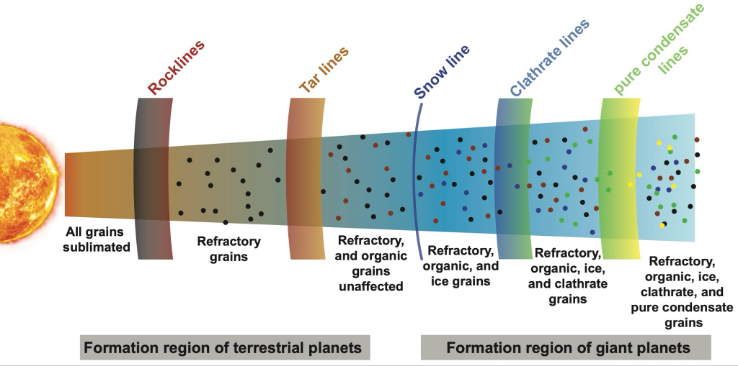
Figure 1. Thermochemical transitions in the PSN. Radial temperature–pressure gradients define rock, tar, snow, clathrate, and ice lines that control the composition of solids and the distribution of carbon among refractory, organic, and volatile reservoirs. Saturn’s position relative to these transitions determines the material incorporated during its growth and influences its present composition.


Tracing Saturn’s Metallicity Back to the Protosolar Nebula

Saturn’s supersolar metallicity, best reflected by its enhanced C/H ratio [12], likely records the chemical evolution of the protosolar nebula (PSN) at its formation location and epoch. In evolving disks, volatile redistribution near ice lines can enrich both vapor and solid phases through condensates, clathrates, and refractory organic-rich material. Saturn’s enrichment may thus result from a combination of supersolar vapors and solids, shaped by disk transport, formation timing, and the balance between gas and solid accretion (Fig. 1).

Each pathway predicts distinct chemical and isotopic fingerprints only testable by in situ measurements. Vapor-dominated accretion would enhance volatile elemental ratios while preserving near-nebular noble-gas abundances and isotopic compositions. Accretion of condensates or clathrates would produce correlated enrichments in heavy noble gases (Ar, Kr, Xe), directly probing clathration efficiency and formation temperature. Refractory organic delivery could alter elemental ratios and shift isotopic tracers such as 14N/15N and D/H away from nebular values. High-precision probe measurements would therefore discriminate between gas-phase enrichment, icy/clathrate delivery, refractory-dominated accretion, or mixtures thereof.

Saturn Probe and Satellite Constraints on Giant Planet Formation

Elemental and isotopic measurements across the Saturnian satellite system provide key context for interpreting Saturn’s formation history. Enceladus’s plume reveals H2O, CO2, organics, and H2, while its D/H ratio is consistent with cometary values inferred for most Saturnian icy satellites (D/H ~ 2–3 × 10⁻⁴) [13–15]. Titan provides additional constraints: its atmosphere is strongly depleted in primordial heavy noble gases relative to solar abundances [16], and its 14N/15N ratio (~167) is far lower than Jupiter’s (~435) measured by the Galileo probe [17]. These signatures suggest that nitrogen in the Saturnian system was incorporated in a chemically processed, possibly ice-rich or organic-bearing form rather than as nebular N2. The forthcoming Dragonfly mission will further refine these constraints through in situ analyses of Titan’s atmosphere and surface chemistry. Combined with future Saturn probe measurements, these data would provide a system-level framework to distinguish enrichment inherited from the PSN from processes operating during planet and satellite formation.

References

[1] Guillot, T. (2005), AREPS, 33, 493.

[2] Helled, R. (2011), ApJL, 735, L16.

[3] Vazan, A. et al. (2016), ApJ, 829, 118.

[4] Militzer, B. et al. (2019), ApJ, 879, 78.

[5] Mankovich, C.R. & Fuller, J. (2021), Nat. Astron., 5, 1103.

[6] Atreya, S.K. et al. (2022), arXiv:2205.06914.

[7] Fletcher, L.N. et al. (2009), Icarus, 199, 351.

[8] Miguel, Y. et al. (2022), A&A, 662, A18.

[9] Wong, M.H. et al. (2024), SSRv, 220, 15.

[10] Mousis, O. et al. (2016), P&SS, 130, 80.

[11] Howard, S. et al. (2024), A&A, 689, A15.

[12] Mousis, O. et al. (2009), ApJ, 696, 1348.

[13] Waite, J.H. et al. (2009), Nature, 460, 487.

[14] Clark, R.N. et al. (2019), Icarus, 321, 791.

[15] Brown, M.E. et al. (2025), PSJ, 6.

[16] Niemann, H.B. et al. (2005), Nature, 438, 779.

[17] Owen, T. et al. (2001), ApJ, 553, L77-L79.


How to cite: Mousis, O., Canup, R., Rhoden, A., Atkinson, D., Atreya, S., Helled, R., Hofstadter, M., Guillot, T., Mankovich, C., Moses, J., and Wong, M.: Future Entry Probe Measurements as Constraints on Saturn’s Formation Environment, Europlanet Science Congress 2026, The Hague, The Netherlands, 7–11 Sep 2026, EPSC2026-500, https://doi.org/10.5194/epsc2026-500, 2026.

09:24–09:36
|
EPSC2026-927
|
On-site presentation
Tristan Guillot

Jupiter's visible zonal winds reach 140 m/s near the equator. Thanks to Juno gravity measurements, we know that they extend to about 3000 km, on cylinders. I will show that this leads to considerable shear, accounting for some of the main features of its atmosphere, namely the absence of storms in the equatorial region and conversely the intense lightning seen at higher latitudes by Juno's MWR instrument. 

How to cite: Guillot, T.: Jupiter's sheared atmosphere, Europlanet Science Congress 2026, The Hague, The Netherlands, 7–11 Sep 2026, EPSC2026-927, https://doi.org/10.5194/epsc2026-927, 2026.

09:36–09:48
|
EPSC2026-651
|
ECP
|
On-site presentation
Nimrod Gavriel, Keren Duer-Milner, Eli Galanti, Fabiano A. Oyafuso, Cheng Li, Steven M. Levin, Scott J. Bolton, and Yohai Kaspi

In rapidly rotating planets, convection driven by residual heat from planetary formation is predicted to organize into columnar circulations aligned with the rotation axis. Such motions have long been proposed to play a central role in giant-planet dynamics, including the maintenance of Jupiter's equatorial superrotation and adjacent westward jets, but their expected depth makes them difficult to observe directly. We analyze microwave brightness-temperature measurements from the Juno Microwave Radiometer (MWR), using multiple channels that probe atmospheric layers down to approximately 100 bar in Jupiter's equatorial region. The data reveal coherent hemispheric asymmetries and characteristic spatial scales consistent with expectations from rapidly rotating deep convection. Comparisons with deep convection simulations reproduce similar signatures and support the interpretation. Cross-depth correlations further suggest axially extended, tilted convective structures. Together, these results provide observational constraints on the geometry and spacing of Jupiter's deep convective motions and their connection to the planet's large-scale atmospheric circulation.

How to cite: Gavriel, N., Duer-Milner, K., Galanti, E., Oyafuso, F. A., Li, C., Levin, S. M., Bolton, S. J., and Kaspi, Y.: Evidence for Tilted Columnar Cells Driving Jupiter's Equatorial Jets, Europlanet Science Congress 2026, The Hague, The Netherlands, 7–11 Sep 2026, EPSC2026-651, https://doi.org/10.5194/epsc2026-651, 2026.

09:48–10:00
|
EPSC2026-723
|
On-site presentation
Yuchen Lian, Pengshuo Duan, and Dali Kong

Gaseous giants are characterized by their deep atmospheres, which lack clear boundaries with their interiors; therefore, their internal states could directly influence atmospheric dynamics. So far, most modeling studies have considered deep convection as the primary mechanism by which the interior influences atmospheric dynamics. In this work, we propose another possible mechanism that might crucially determine the appearance of gaseous giants’ atmospheric cloud-top jet winds, tracing them to a typical hydromagnetic wave (the so-called equatorial Magnetic-Archimedes-Coriolis wave) generated within the stably stratified, strongly magnetized helium rain layer. The associated thermal perturbations can propagate upward through the convective molecular hydrogen envelope, eventually affecting the atmospheric thermal structure—the zonal inhomogeneities that are conducive to the formation of the eastward atmospheric equatorial jet (superrotation). Our results have important implications for understanding the equatorial dynamics of gaseous giants. This mechanism could also help explain the equatorial westward jets (subrotation) observed on Uranus and Neptune, which lack the helium rain layers.

How to cite: Lian, Y., Duan, P., and Kong, D.: A Possible Mechanism to Explain the Prograde Equatorial Jet of a Jupiter-like Gaseous Giant, Europlanet Science Congress 2026, The Hague, The Netherlands, 7–11 Sep 2026, EPSC2026-723, https://doi.org/10.5194/epsc2026-723, 2026.

Orals MON2: Mon, 7 Sep, 11:00–12:30 | Room Jupiter (Jazz 1 & 2)

Chairpersons: Sandrine Guerlet, Deborah Bardet
Troposphere and stratosphere
11:00–11:15
|
EPSC2026-44
|
solicited
|
On-site presentation
Patrick Irwin, Asier Anguiano-Arteaga, Michelle Colantoni, Joseph Penn, Santiago Perez-Hoyos, Davide Grassi, and Charlotte Alexander

Analysing observations of Jupiter made by VLT/MUSE (0.475 – 0.933 μm), Cassini/VIMS (0.40 – 5.15 μm), and Juno/JIRAM (2 – 5 μm), we present early results of a new combined cloud-ammonia profile model for Jupiter's equatorial atmosphere. We find this model to be consistent with all observations considered, at a range of observation geometries, within the Equatorial Zone (EZ), the North Equatorial Belt (NEB) and a North Equatorial Dark Feature (NEDF), also known as a '5-micron-hotspot'. Preliminary results suggest the presence of three main layers: 1) a deep 'Cloud-1' at 1-2 bar; 2) an upper 'Cloud-2' in the upper troposphere based at ~0.55 bar; and 3) a layer of chromophore particles situated within the Cloud-1 layer, responsible for the blue-absorption at visible wavelengths.  Our best-fit ammonia profile is closely linked with our cloud profile, with Cloud-1 coinciding with a sharp drop in ammonia abundance, perhaps associated with the formation of a H2O-NH3 'mushball' cloud, or an ammonium hydrosulphide (NH4SH) cloud, or both, and Cloud-2 coinciding with the ammonia condensation level.

We find the bulk of the cloud opacity in Jupiter’s atmosphere to be in the Cloud-1 layer, based at 1-2 bar and composed of relatively large particles (r ~ 10 μm), which are highly scattering at visible wavelengths to allow sunlight to penetrate and be Rayleigh-scattered from the deeper atmosphere, but more absorbing at 5 μm. The belt/zone difference at 5 μm is accounted for by changes in the opacity of Cloud-1 and also the single-scattering albedo of these particles. We find the Cloud-2 layer, based at the ammonia condensation level, to be approximately 10 times less opaque than Cloud-1 and have an absorption band near 3 μm, which is consistent with this layer having a significant opacity of large (r ~ 10 μm) ammonia ice particles.

We will present preliminary insights into the spatial distribution of these clouds over the regions considered and their implications for our understanding of Jupiter’s chromophores and upper-level hazes.

How to cite: Irwin, P., Anguiano-Arteaga, A., Colantoni, M., Penn, J., Perez-Hoyos, S., Grassi, D., and Alexander, C.:  Vertical Distribution of Cloud and Ammonia in Jupiter’s equatorial atmosphere revealed by co-analysis of VLT/MUSE, Cassini/VIMS and Juno/JIRAM  , Europlanet Science Congress 2026, The Hague, The Netherlands, 7–11 Sep 2026, EPSC2026-44, https://doi.org/10.5194/epsc2026-44, 2026.

11:15–11:30
|
EPSC2026-248
|
solicited
|
On-site presentation
Leigh N. Fletcher, Oliver King, Michael H. Wong, Pablo Rodriguez Ovalle, Simon Toogood, Imke de Pater, Gordon L. Bjoraker, Ricardo Hueso, Philip Marcus, Glenn Orton, James Sinclair, Thierry Fouchet, Arrate Antunano, Shinji Mizumoto, Rob Bullen, and John Rogers

Jupiter’s large angular size, brightness, and rapid rotation made it an ideal test for JWST observations during the first cycle of science operations (2022-23).  A combination of guaranteed time and early-release science programmes revealed new insights into Jupiter’s jet streams [1], auroras [2], low-latitude ionosphere [3], polar chemistry [4], and the vertical structure of the Great Red Spot [5, 6].  However, spectroscopic mapping coverage remained limited, due to the small fields-of-view of JWST’s integral field spectrometers (3-6”) compared to Jupiter’s diameter (~45”).  We addressed this via a trio of Cycle-4 programmes in February 2026, coordinating a campaign including NIRCam (1-5 µm imaging), NIRSpec/IFU (1.8-5.3 µm spectroscopy) and MIRI/MRS (4.9-28.5 µm spectroscopy), combined with amateur observers (providing visible-light context), professional observatories (VLT), and overlapping with Jupiter flybys by NASA’s Juno mission.  This presentation provides a first look at the dataset acquired in 2026.

JWST Observations:  GO6840 (14hrs, February 21-22, 2026, PI: Wong) acquired a 6-tile NIRSpec/IFU mosaic of Oval BA, Jupiter’s second-largest anticyclone, followed by two sets of NIRCam global imaging (spaced ~10 hours apart for tracking of cloud features), and followed by a 3-tile mosaic of Oval BA with MIRI/MRS.  GO8173 (16hrs, February 20, 2026) acquired MIRI/MRS observations of Jupiter’s poles and mid-IR auroral emissions, intended to map exogenous species provided to Jupiter’s stratosphere, focussing on the evolution of stratospheric H2O, CO2 and HCN that were initially delivered by comet Shoemaker-Levy 9 in 1994.  These were combined with GO6865 (24hrs, February 27-28, PI: Fletcher), which acquired a pole-to-pole MIRI/MRS scan as Jupiter rotated (13 distinct pointings), providing JWST’s first “global” map of 3D temperatures and gaseous composition.  These were scheduled to be as close as possible to Juno’s 81st perijove (February 25, 2026) to enable comparison of temperatures and composition with Juno’s close-in remote sensing and radio occultations.  All JWST spectroscopic data have been reduced via a custom pipeline [7] that reduces the effects of saturation, cleans artefacts from flat-fielding and cube-building phases, and then maps the data using PlanetMapper [8].

Amateur Support:  Interpretation of the JWST data will benefit significantly from a world-wide campaign of ground-based observations acquired throughout February 2026, revealing how the atmospheric phenomena observed in the infrared shifted and evolved during this period.  These global-scale visible-light images were collected through repositories like the Planetary Virtual Observatory and Laboratory (PVOL, http://pvol2.ehu.eus/pvol2/), the Association of Lunar and Planetary Observers (ALPO, https://alpo-astronomy.org/), or the ALPO-Japan site (https://alpo-j.sakura.ne.jp/indexE.htm), and then reprojected into maps via WinJUPOS. 

Global MIRI Results – Belts, Zones, Auroras:  The combined dataset reveals Jupiter’s banded structure from pole to pole, with spectroscopic inversions deriving 3D temperatures in the troposphere and stratosphere; tropospheric volatiles (NH3, H2O), clouds, and disequilibrium species (PH3, AsH3, CO); stratospheric hydrocarbons (CH4 and its derivatives) and exogenic species (CO2, H2O, HCN).  North-south temperature contrasts are largest at the peaks of the zonal winds, confirming vertical windshear on the east-west flows.  Auroral heating is evident over both poles, including diffuse warmth within the northern oval (observed via CH4 emission), and intriguing observations of a distinct auroral arc at 10.5 µm (ethylene emission).  The zonal temperature field will be compared to (i) recent Juno ratio occultation measurements [9] and (ii) the most recent space-based infrared thermal maps from Cassini/CIRS in 2000 [10].  The tropospheric composition (particularly NH3, PH3, and H2O) will be used to search for robust evidence of rising and falling motions on the scale of Jupiter’s belts and zones.

Regional MIRI Results – Rifts, Storms, Vortices:  Despite the small field-of-view of MIRI/MRS, there is significant structure observed in each tile, including rifting, plumes and hotspots (dark formations) within the North Equatorial Belt; discrete white spots and wave patterns in the North-North Temperate Domain; Folded Filamentary Structure at southern high latitudes; and the internal structure of cyclonic segments (elongated brown features) in the South Temperate Belt. In addition, the mosaic of Oval BA captured several Anticyclonic White Ovals (A2 and A3) in the South-South Temperate Belt, meaning that we now have spectroscopic maps of three classes of anticyclones, from the largest (the Great Red Spot), to the intermediate-sized Oval BA, to the smaller white ovals.  Preliminary inspection reveals that the width of Oval BA changes with altitude in the troposphere, though spectral inversions are needed to disentangle thermal and aerosol effects. MIRI will allow us to indirectly measure 3D windshear over these ovals to understand how their peripheral winds change with altitude, to be compared to NIRCam’s direct windshear measurements (NIRCam has sensitivity to high-altitude haze features above the anticyclone’s main cloud deck).

By combining these three independent programmes (all acquired within a few days of one another) with ground-based context imaging, we provide the most comprehensive JWST view of Jupiter’s atmospheric dynamics and chemistry to date. 


References:  [1] Hueso et al., 2023, Nature Astronomy (10.1038/s41550-023-02099-2); [2] Nichols et al., 2025, Nature Communications (10.1038/s41467-025-58984-z); [3] Melin et al., 2023, Nature Astronomy (10.1038/s41550-024-02305-9); [4] Rodriguez-Ovalle et al., 2024, Astronomy & Astrophysics (10.1051/0004-6361/202451453); [5] Harkett et al., 2024, JGR: Planets (10.1029/2024JE008415); [6] Biagiotti et al., 2025, Astronomy & Astrophysics (10.1051/0004-6361/202554552); [7] King et al., 2023, RNAAS (10.3847/2515-5172/ad045f); [8] King et al., 2023, Journal of Open Source Software (10.21105/joss.05728); [9] Smirnova et al., 2026, Astronomy & Astrophysics (10.1051/0004-6361/2025568196); [10] Fletcher et al., 2016, Icarus, (10.1016/j.icarus.2016.06.008). 

How to cite: Fletcher, L. N., King, O., Wong, M. H., Rodriguez Ovalle, P., Toogood, S., de Pater, I., Bjoraker, G. L., Hueso, R., Marcus, P., Orton, G., Sinclair, J., Fouchet, T., Antunano, A., Mizumoto, S., Bullen, R., and Rogers, J.: The JWST-Jupiter 2026 Campaign: Stripes, Vortices, and Auroras, Europlanet Science Congress 2026, The Hague, The Netherlands, 7–11 Sep 2026, EPSC2026-248, https://doi.org/10.5194/epsc2026-248, 2026.

11:30–11:42
|
EPSC2026-908
|
ECP
|
On-site presentation
Pablo Rodríguez-Ovalle, Leigh N. Fletcher, Rose Peybernes, Mike Wong, Thierry Fouchet, Sandrine Guerlet, Thibault Cavalié, Vincent Hue, Manuel López-Puertas, James A. Sinclair, Imke de Pater, Oliver King, and Simon Toogood

The James Webb Space Telescope has opened a new window into the study of Giant Planets in the Solar System. During its first cycle, JWST observed Jupiter and its moons as part of the Early Release Science program ERS1373. JWST studied –Among its multiple observations – Jupiter using NIRCam imaging [1] together with NIRSpec and MIRI IFU modes [2–4], demonstrating JWST’s extraordinary capability to probe the stratospheric and thermospheric structure of the giant planet. However, these very first observations, specifically for MIRI, specifically aimed at the south polar region and only partially sampled the southern auroral oval itself, with only one observation directly probing the polar auroral region, interior of the main oval. 

A new observation campaign for Jupiter was carried out with JWST in February 2026, which overcame these coverage limitations. The main goal of this campaign was to  produce the most extensive and comprehensive dataset of Jupiter’s atmosphere obtained so far. This campaign combines observations from programs GO8173, and GO6865, providing a complete meridional coverage of the planet, and allowing systematic observations both inside and outside the northern auroral oval with the MIRI/MRS instrument. The southern auroral oval could not be directly observed, being only partially covered. However, the combined dataset offers a unique opportunity to directly compare auroral and non-auroral regions under similar observing conditions in both poles.

The new observations have been corrected using improved preprocessing techniques specifically developed for JWST/MIRI data. Desaturation routines now allow us to recover the spectroscopic information up to 20 μm, while maintaining reliable photometric calibration up to approximately 15.5 μm. In addition, a new flat-field correction algorithm has been implemented to mitigate spectral-shift artifacts that affect differently within the detector Field Of View. This work will present the full preprocessing pipeline and discuss the impact of these corrections on the quality of the acquired spectra. The cleaned spectra were then analyzed using a radiative transfer code coupled to an inversion algorithm that has already been tested in previous studies for Jupiter and Saturn’s atmospheres datasets [5].

Temperature fields were then retrieved using the CH4​ ν4​ emission band. This spectral region is particularly sensitive to the atmospheric layers around the 50 mbar up to the 1 μbar pressure level when observing bright auroral regions, enabling the study of Jupiter’s upper atmosphere in those cases. In regions with sufficient thermospheric sensitivity such as the auroral regions, simultaneous retrievals of temperature and homopause altitude were performed following the methodology described in [3,6]. From these analyses, we derived temperature profiles spanning pressures from approximately 30 mbar down to 0.01 mbar, and we explore different atmospheric scenarios to constrain the location and variability of the homopause in both polar regions. Our preliminary results reveal clear thermal contrasts between auroral and non-auroral regions, with enhanced temperatures and vertical structure variations inside the auroral ovals compared to the non-quiescent regions. The retrievals also suggest substantial differences in homopause altitude when comparing regions inside and outside the ovals, potentially linked to differences in auroral energy deposition and atmospheric circulation. These findings provide new constraints on the coupling between Jupiter’s thermosphere and stratosphere and highlight the strong dynamical influence of auroral processes on the polar atmosphere.

Once the temperature structure was obtained, we retrieved the abundances of several hydrocarbons, including C2​H2​, C2​H6​, and C6​H6​. Mapping the spatial distribution of these species in the polar regions is needed for interpreting the abundances of the exogenic molecules, since many of their spectral signatures overlap with these hydrocarbon emission features. The resulting abundance maps are compared with the meridional distributions predicted by photochemical models [7], allowing us to infer ion-neutral chemistry processes. Early analyses indicate localized enhancements and departures from purely photochemical expectations, particularly at high latitudes, supporting the presence of strong auroral chemical pathways.

A major scientific goal of this work is the study of the exogenic species CO2​, H2​O, and HCN, whose abundances can be strongly influenced by polar atmospheric processes and, more specifically, auroral activity [8, 9]. Constraining the spatial variability of these molecules in the polar regions is essential for identifying how the exogenous molecules in Jupiter’s atmosphere can evolve with time. In that line, we will present our future plans for retrieving exogenic species across the entire planet, with particular interest in the mapping of the polar regions [10]. We will compare the abundances of CO2​, H2​O, and HCN inside and outside the auroral ovals, produce polar maps of CO2​ and H2​O, and retrieve the full meridional distribution of HCN column densities. We aim to analyze these results alongside the spatial distribution of Jupiter’s stratospheric polar aerosols, providing a broader picture of the interaction between auroral activity, atmospheric chemistry, and aerosol formation in Jupiter’s upper atmosphere.


[1] Hueso, R. et al. (2023). Nature Astronomy, 7(11), 1294–1302. https://doi.org/10.1038/s41550-023-02099-2

[2] Biagiotti, F. et al. (2025). Astronomy & Astrophysics, 696, A10. https://doi.org/10.1051/0004-6361/202554552

[3] Rodríguez-Ovalle, P. et al. (2024). J. Geophys. Res. Planets, 129(11), e2024JE008299. https://doi.org/10.1029/2024JE008299

[4] Harkett, J. et al. (2024). J. Geophys. Res. Planets, 129(12), e2024JE008415. https://doi.org/10.1029/2024JE008415

[5] Fouchet, T. et al. (2016). Icarus, 277, 196–214. https://doi.org/10.1016/j.icarus.2016.04.030

[6] Sinclair, J. A. et al. (2023). Planetary Science Journal, 4(5), 95. https://doi.org/10.3847/PSJ/accb95

[7] Moses, J. I. et al. (2005). J. Geophys. Res. Planets, 110(E8), E08001. https://doi.org/10.1029/2005JE002411

[8] Rodriguez-Ovalle, P. et al. (2025). Astronomy & Astrophysics, 694, A123. https://doi.org/10.1051/0004-6361/202451453

[9] Cavalié, T. et al. (2023). Nature Astronomy, 7(11), 1284–1293. https://doi.org/10.1038/s41550-023-02016-7

[10] Hue, V. et al. (2025). Space Science Reviews, 221(1), 7. https://doi.org/10.1007/s11214-024-01119-5

How to cite: Rodríguez-Ovalle, P., Fletcher, L. N., Peybernes, R., Wong, M., Fouchet, T., Guerlet, S., Cavalié, T., Hue, V., López-Puertas, M., Sinclair, J. A., de Pater, I., King, O., and Toogood, S.: JWST Cycle 4 observations of Jupiter’s polar region:Constraining temperature and hydrocarbon abundances, Europlanet Science Congress 2026, The Hague, The Netherlands, 7–11 Sep 2026, EPSC2026-908, https://doi.org/10.5194/epsc2026-908, 2026.

11:42–11:54
|
EPSC2026-47
|
ECP
|
On-site presentation
José Ribeiro, Pedro Machado, Santiago Pérez-Hoyos, Asier Anguiano-Arteaga, and Patrick Irwin

The origin and vertical distribution of Jupiter’s red coloration remain uncertain, despite multiple proposed aerosol models. Laboratory work (Carlson et al., 2016) showed that photolyzed ammonia and acetylene can form a red compound consistent with Jupiter’s colours, motivating the “universal chromophore” hypothesis (Sromovsky et al., 2017), and the “Crème Brûlée” model (Baines et al., 2019), which places a thin absorber above the ammonia clouds. Later HST and VLT studies (Pérez‑Hoyos et al., 2020; Braude et al., 2020) suggested a more vertically extended, less blue‑absorbing material, while recent analyses of the Great Red Spot and Oval BA indicate the presence of two distinct colouring agents: a universal‑chromophore absorber and a deeper UV‑absorbing aerosol (Anguiano‑Arteaga et al., 2021, 2023). These findings highlight persistent ambiguity in Jovian aerosol composition and structure.

To investigate this, we analysed 2019 Jupiter observations from CARMENES (The Calar Alto High-Resolution search for M dwarfs with Exoearths with Near-infrared and optical Échelle Spectrographs), (0.52–1.71 μm). Since no calibration star was available, we calibrated the spectra using Saturn’s B ring and Cassini/VIMS reflectivity (Cuzzi et al., 2009), achieving agreement with published Jupiter spectra to within 10% (Clark, R.N., McCord, T.B., 1979; Mendikoa, I., et al., 2017; Irwin, P.G., et al., 2018).

Using 64 VIS–NIR observation pairs, we performed a Minnaert limb‑darkening analysis and generated synthetic spectra for five regions. These were used in NEMESIS retrievals with three aerosol models. Across all models, the highest‑altitude aerosol layer dominated the spectral behaviour, with particle size, cloud‑base abundance, and pressure level strongly influencing the fits. Model B (Braude et al., 2020) produced the lowest χ²/Nfree values, but no model fully reproduced the observations, likely due to the limited wavelength range, which lacks constraints on deeper clouds.

The models diverged in retrieved particle sizes and cloud‑base pressures, with several results, such as extremely small tropospheric particles or overly large stratospheric particles, indicating physical inconsistencies. Model A’s tropospheric haze base aligns with Galileo probe measurements (Sromovsky and Fry, 2002); Model C retrieves a cloud base level near the NH₄SH level predicted by Atreya (1998), deeper than CIRS detections (Matcheva et al.,2005) but within the range of Baines et al. (2019), with implausible particle sizes.

Overall, the study shows that CARMENES can deliver high‑quality, flux‑calibrated planetary spectra, but also that broader spectral coverage is essential to resolve Jupiter’s chromophore composition and aerosol vertical structure.


Figure 1: Location of the spectra used to perform the Minnaert limb-darkening approximation for each region considered in this study. Red for EZ, yellow for NEB, green for SEB, pink for SEB transition and blue for NEB transition. The Jupiter AGC image represented corresponds only to the spectra of the EZ whose longitude was closest to 0º.


Figure 2: Comparison between observed and modelled spectra and residuals for EZ using model B]{Comparison between observed (blue) and modelled (red) spectra (left column) and comparison between differences (red) and a priori errors (black) (right column) for the EZ using model B, with the grey shaded areas corresponding to telluric absorption. The top row corresponds to nadir (incidence and emission angle = 0º) and the bottom row to limb (incidence and emission angle = 61.45º).


Figure 3: Comparison between the a priori aerosol vertical profiles and the retrieved profiles for every region for models A and B. We compare the optical depth/atm at 0.90 μm of model B with all three aerosol populations considered and model A's stratospheric and tropospheric hazes. The horizontal dashed line corresponds to 0.15 atm, separating model B's deep cloud layer from the haze.


References:

  • Carlson, R. W., et al. (2016). Chromophores from photolyzed ammonia reacting with acetylene: Application to Jupiter's Great Red Spot. Icarus, 274, 106–115.
  • Sromovsky, L. A., et al. (2017). A possibly universal red chromophore for modeling color variations on Jupiter. Icarus, 291, 232–244.
  • Baines, K. H., et al. (2019). The visual spectrum of Jupiter's Great Red Spot accurately modelled with aerosols produced by photolyzed ammonia reacting with acetylene. Icarus, 330, 217–229.
  • Pérez-Hoyos, S., et al. (2020). Color and aerosol changes in Jupiter after a North temperate belt disturbance. Icarus, 132, 114021.
  • Braude, A. S., et al. (2020). Colour and tropospheric cloud structure of Jupiter from MUSE/VLT: Retrieving a universal chromophore. Icarus, 338, 113589.
  • Anguiano-Arteaga, A., et al. (2021). Vertical Distribution of Aerosols and Hazes Over Jupiter's Great Red Spot and Its Surroundings in 2016 From HST/WFC3 Imaging. Journal of Geophysical Research: Planets, 126, e2021JE006996.
  • Anguiano-Arteaga, A., et al. (2023). Temporal variations in vertical cloud structure of Jupiter's Great Red Spot, its surroundings and Oval BA from HST/WFC3 imaging. Journal of Geophysical Research: Planets, 128, e2022JE007427.
  • Irwin, P., et al. (2008). The NEMESIS planetary atmosphere radiative transfer and retrieval tool. J. Quant. Spectrosc. Radiat. Transf., 109, 1136–1150.
  • Rodgers CD. (2000). Inverse methods for atmospheric sounding: theory and practice. Singapore: World Scientific.
  • Cuzzi, J., et al., 2009. Ring Particle Composition and Size Distribution. Springer Netherlands, Dordrecht. pp. 459–509.
  • Clark, R.N., McCord, T.B., 1979. Jupiter and Saturn: Near-infrared spectral albedos. Icarus 40, 180–188.
  • Mendikoa, I., et al., 2017. Temporal and spatial variations of the absolute reflectivity of Jupiter and Saturn from 0.38 to 1.7 𝜇m with planetcam-upv/ehu. A&A 607, A72.
  • Irwin, P.G., et al., 2018. Analysis of gaseous ammonia (NH3) absorption in the visible spectrum of Jupiter. Icarus 302, 426–436.
  • Matcheva, K.I., Conrath, B.J., Gierasch, P.J., Flasar, F.M., 2005. The cloud structure of the jovian atmosphere as seen by the Cassini/CIRS experiment. Icarus 179(2), 432–448.
  • Sromovsky, L., Fry, P., 2002. Jupiter’s cloud structure as constrained by Galileo probe and HST observations. Icarus 157 (2), 373–400.

How to cite: Ribeiro, J., Machado, P., Pérez-Hoyos, S., Anguiano-Arteaga, A., and Irwin, P.: Final results: Jovian upper clouds and hazes from visible and near infrared spectroscopy using CARMENES, Europlanet Science Congress 2026, The Hague, The Netherlands, 7–11 Sep 2026, EPSC2026-47, https://doi.org/10.5194/epsc2026-47, 2026.

11:54–12:06
|
EPSC2026-627
|
ECP
|
On-site presentation
Mikel Sánchez-Arregui, Arrate Antuñano, Leigh N. Fletcher, Ricardo Hueso, Simon Toogood, Oliver R. T. King, Thomas Greathouse, and Agustín Sánchez-Lavega

Long-term observations of Jupiter in the thermal IR have shown that the equatorial stratospheric temperatures oscillate on multi-year time-scales [1-2]. This oscillation affects not only the temperatures, but also the winds between the North and South Equatorial Belts at pressure levels of 0.1-40 mbar. This Jupiter Equatorial Stratospheric Oscillation (JESO) is apparently unrelated to seasons as Jupiter’s rotation axis is tilted by only 3.1°, and the equatorial stratosphere shifts from warm to cool temperature patterns with a variable period of 3.9-5.7 years, significantly different from to Jupiter’s orbital period of 11.9 Earth years. Previous studies based on analyses of infrared observations have shown that the JESO experiences major disruptions of its periodicity, principally related to tropospheric “Global Upheavals” [3] and large convective outbreaks developing in the troposphere away from the equator [4]. Numerical simulations reveal that vertically propagating gravity waves play a vital role in the nature of the oscillation depositing additional momentum from the troposphere up to the stratosphere [5-6]. The vertical extension of the oscillation is not well determined, since retrieving temperatures above or below the 1-20 mbar pressure range becomes more difficult. However, recent works that gather four decades of ground-based infrared observations reveal that the upper-tropospheric temperatures could also be affected by the JESO phenomena, thus coupling the tropospheric and stratospheric activity [7-8].

The first Jupiter observations made with the James Webb Space Telescope discovered an intense narrow equatorial jet located in the lower stratosphere (50-200 mbar), and it has been suggested to be a deep counterpart of JESO [9]. Additionally, a recent study of the variability of the equatorial winds and haze reflectivity in the upper troposphere suggest that the stratospheric jet could be detectable with methane images that probe the elevated hazes at 200-400 mbar [10]. Furthermore, changes in haze reflectivity from 2019 to 2022 suggest that a change in the hazes’ altitude could be the reason to detect the jet with images that sense deeper than the lower stratosphere.

In this work, we analyse mid-infrared IRTF-TEXES observations from 5 to 20 microns obtained over a full Jovian year to characterize the thermal state of Jupiter’s equatorial atmosphere. These multi-wavelength spectral cubes probe different altitudes, allowing the retrieval of temperatures from the stratosphere to the mid-troposphere, chemical distributions and aerosol opacity at the ammonia cloud level. We will show derived atmospheric properties through retrievals of the vertical structure of the atmosphere with the NEMESIS radiative-transfer and retrievals codes [11-12]. The spectroscopic inversions provide high resolution 3D profiles of temperatures, composition and aerosols that enable the study of a possible extension of the stratospheric oscillation to deeper levels, as well as to delve into the nature of brightness changes in the observed hazes. These results extend previous long-term studies [4,7-8] and will be essential to unveil the relation between stratospheric and tropospheric phenomena at the equator, and, therefore, the potential links between the JESO, the equatorial jet, and convective tropospheric activity.


References

[1] Leovy, C., et al. Nature 354, 380–382 (1991). [2] Orton, G. S., et al. (1991). Science, 252 (5005), 537-542. [3] Antuñano, A, et al. Nat Astron 5, 71–77 (2021). [4] Giles, R. S., et al. (2020). Icarus, 350, 113905. [5] Cosentino, R. G., et al. (2017). Journal of Geophysical Research: Planets, 122, 2719–2744. [6] Cosentino, et al. The Planetary Science Journal. 1. 63 (2020). [7] Orton, G. S et al., Nature Astronomy, 7, 190-197 (2023). [8] Antuñano, A., et al., Journal of Geophysical Research: Planets, 128 (12) (2023). [9] Hueso, R., et al. Nat Astron 7, 1454–1462 (2023). [10] Sánchez-Arregui, M., et al. (2025). Journal of Geophysical Research: Planets, 130, e2025JE009332. [11] P.G.J. Irwin et al. In: Journal of Quantitative Spectroscopy and Radiative Transfer 109.6 (Apr. 2008), pp. 1136–1150. [12] Leigh N. Fletcher, et al., Icarus, Volume 278, 2016, Pages 128-161.

How to cite: Sánchez-Arregui, M., Antuñano, A., Fletcher, L. N., Hueso, R., Toogood, S., King, O. R. T., Greathouse, T., and Sánchez-Lavega, A.: Characterization of temperatures, clouds and aerosols in Jupiter from the troposphere to the stratosphere for a full Jovian year with IRTF-TEXES., Europlanet Science Congress 2026, The Hague, The Netherlands, 7–11 Sep 2026, EPSC2026-627, https://doi.org/10.5194/epsc2026-627, 2026.

12:06–12:18
|
EPSC2026-886
|
ECP
|
On-site presentation
Francesco Biagiotti, Pietro Scarica, Grassi Davide, Alessandro Mura, Cheng Li, Giuseppe Piccioni, Chiara Castagnoli, Alberto Adriani, Christina Plainaki, Federico Tosi, Roberto Sordini, Andrea Cicchetti, Raffaella Noschese, and Scott Bolton

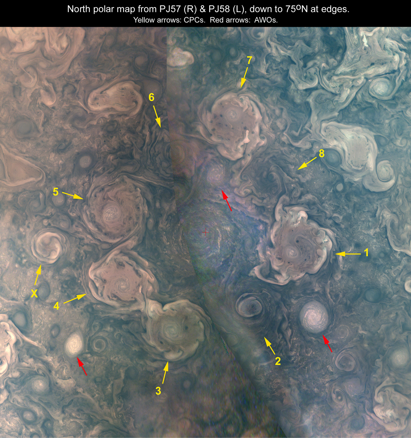
The polar regions of Jupiter represent one of the most complex dynamical environments in the solar system, characterized by a series of persistent, geometrically organized cyclonic structures [1]. Despite extensive observation, the fundamental origin, vertical structure, and chemical composition of these circumpolar cyclones (CPCs) remain key open questions in planetary science. Moreover, the polar caps are recognized as regions where high-energy particles, accelerated by Jupiter’s powerful magnetic field, drive intense aurorae and interact directly with atmospheric gaseous species in the upper atmospheric layers [2,3]. A primary consequence of this interaction is the presence of dense, thick stratospheric hazes that produce prominent signals in the ultraviolet (UV) [4] and can be effectively probed at near-infrared (NIR) wavelengths [5,6,7]. However, the specific composition and vertical distribution of the polar troposphere have historically remained elusive due to the extreme viewing geometries and the limitations of previous instrumentation.

The Jovian Infrared Auroral Mapper (JIRAM) provided the first preliminary maps of optical depth and minor species concentrations derived from 5  μm radiance measurements [8]. These early findings suggested that while the cyclones are optically thick, their average values are significantly lower (by a factor of 2 to 3) than those observed in equatorial regions. Nevertheless, the concentrations of minor species within these regions appeared largely comparable to equatorial values.

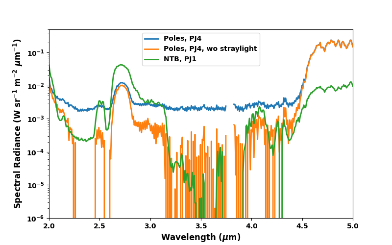
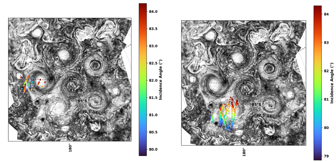
In this work, we present the first rigorous multiple-scattering atmospheric retrieval analysis of JIRAM spectra captured at the poles. Our objective is to characterize the polar troposphere in terms of aerosol vertical structure, particulate composition, and gaseous ammonia (NH3) content. We focused our investigation on the data acquired during JIRAM’s fourth perijove passage (PJ4). To ensure the integrity of the multiple-scattering retrievals and avoid the instabilities common to extreme viewing conditions, we implemented a strict selection criterion, retaining only spectra acquired at incidence angles lower than 85°. Under these constraints, the spatial resolution was found to be sufficient for a detailed study of the South Pole, specifically focusing on two distinct cyclones—CPC1 and CPC3—and their immediate surrounding regions, see Fig. 1. Due to the extreme energetic conditions at the poles the selected JIRAM spectra are extremely noisy, mostly because of the presence of a source of stray light, that becomes more significant at the viewing conditions of the polar regions and that we removed using the methods presented in [9]. The resulting reduced spectra reveal solar reflected radiances that are two orders of magnitude lower than equatorial observations and one order of magnitude lower than those recorded at lower latitudes, see Fig. 2.

For the forward modeling and retrieval, we utilized the NASA Planetary Spectrum Generator (PSG) [10], following the multiple-scattering methodology established by [11]. We modeled the solar-reflected spectral region (2.0–3.1 μm) using a discrete three-layer atmospheric scheme: (i) a box-like tropospheric haze layer at ∼ 0.2-0.4 bar, composed of small (0.1–0.3 μm) pure-reflecting particles; (ii) an intermediate Gaussian cloud deck at ∼  0.7 bar, where we tested both tholin-like particulates and pure ammonia ice; and (iii) a deep Gaussian cloud at ∼  1.2 bar with refractive indices consistent with ammonium hydrosulfide (NH4SH). The vertical distribution, density, and effective radii of these aerosols were treated as free parameters, along with the deep concentration and relative humidity of gaseous ammonia.

Our findings yield several insights: (i) in order to model the 2.0-2.4 μm region of the JIRAM spectra we need to include a stratospheric haze as in [5,6,7,]; (ii) the spectral fits do not necessitate the presence of pure ammonia ice particulates within the CPCs; (iii) the deep cloud layers within the CPCs are situated at greater depths (higher pressures) than in surrounding regions, whereas the upper-level clouds exhibit an upward displacement; (iv) the retrieved tropospheric haze and cloud densities are consistently one order of magnitude lower than those at lower Jovian latitudes; (v) the integrated aerosol opacity within the CPC core is higher than in the immediate intra-cyclonic environment; and (vi) retrieved NH3 concentrations are in agreement with MWR data. 

To explain these observations, we propose a dynamical model wherein upwelling within the cyclone core produces adiabatic cooling. This ascending motion must be balanced by compensatory subsidence; the descending air warms adiabatically, shifting the local condensation level downward and causing the deep cloud top to appear deeper in the atmosphere.

While the low tropospheric aerosol density values are consistent with the measured solar radiances and the results of previous NIR retrievals [5], they are not trivial to explain from a theoretical point of view. We explore various sink mechanisms that may govern this environment, including: the tropopause temperature barrier, the over-abundance of cloud condensation nuclei (CCNs), the Clausius-Clapeyron barrier, the inhibition of UV photon penetration, and the potential for rain-out effects.

References:

[1] Adriani A., Mura A., Orton G., Hansen C., Altieri F., et al. 2018, Nature, Volume 555, Issue 7695, pp. 216-219

[2] Hue V., Cavalié T., Sinclair J. A., Zhang X., et al. 2024, Space Science Reviews, Volume 220, Issue 8, id.85

[3] Castagnoli C., Dinelli B. M., Altieri F., Migliorini A., et al. 2025, The Planetary Science Journal, Volume 6, Issue 4, id.93  

[4] Hord C. W., West R. A., Simmons K. E., Coffeen D. L., et al. 1978, Science, Volume 206, No. 4421

[5] Zhang X., West R. A., Banfield D., Yung Y. L., 2013, Icarus, Volume 226, Issue 1, September–October 2013, Pages 159-171 

[6] Banfield D., Conrath B. J., Gierasch P. J., Nicholson P. D., Matthews K., Icarus, Volume 134, Issue 1, July 1998, Pages 11-23

[7] Rodriguez-Ovalle P., Guerlet S., Fouchet T., Harkett J., et al. 2024, A&A, 691, A51 

[8] Adriani A., Bracco A., Grassi D., Moriconi M. L., Mura A., et al. 2020, Journal of Geophysical Research: Planets, Volume 125, Issue 6

[9] Grassi D., Mura A., Castagnoli C., Biagiotti F., et al. 2026, CNSP26 congress

[10] Villanueva G. L., Smith M. D., Protopapa S., Faggi S., Mandell A. M., 2018, J. Quant. Spec. Radiat. Transfer, 217, 86

[11] Biagiotti, F., Grassi, D., Liuzzi, G., et al. 2025, Monthly Notices of the Royal Astronomical Society, staf38

Fig. 1

Fig.2

How to cite: Biagiotti, F., Scarica, P., Davide, G., Mura, A., Li, C., Piccioni, G., Castagnoli, C., Adriani, A., Plainaki, C., Tosi, F., Sordini, R., Cicchetti, A., Noschese, R., and Bolton, S.: Probing the Tropospheric Architecture of Jupiter’s CPCs with Juno/JIRAM: New Constraints on Aerosols and Gaseous Ammonia, Europlanet Science Congress 2026, The Hague, The Netherlands, 7–11 Sep 2026, EPSC2026-886, https://doi.org/10.5194/epsc2026-886, 2026.

12:18–12:30
|
EPSC2026-43
|
On-site presentation
Agustin Sanchez-Lavega, Amy A. Simon, Michael H. Wong, Leigh N. Fletcher, Arrate Antuñano, Ricardo Hueso, Peio Iñurrigarro, Aida Flix-Bellmunt, Enrique García-Melendo, Trevor Barry, Jean-Paul Oger, Glenn S. Orton, Itziar Garate-Lopez, and Arnau Miró

Saturn has a unique long-lived, nearly stationary hexagon wave close to its north pole that is coupled to an intense eastward jet. Despite decades of observation, no similar wave has been reported so far in the southern hemisphere or elsewhere on Saturn. Ground-based and Hubble Space Telescope (HST) images obtained in 2025 revealed the presence of a decagonal wave at planetographic latitudes ~  58°S - 63°S. HST images in 2023 and 2024 showed vertices with weaker albedo contrasts and linear sides of the decagon, implying an evolving phenomenon. The decagon moves eastwards with a velocity of 2.5 m/s relative to System III radio-rotation period, much slower than the zonal jet centered at latitude of 60.5°S that has a peak velocity of 116 m/s. Simultaneously, the position in longitude of its vertices oscillate relative to the mean motion with an average period of 32 days and amplitudes of 4.6°-8.4°. The decagon could be a quasi-geostrophic Rossby wave trapped vertically and confined meridionally by the dominant jet curvature with an intrinsic phase speed of -113 ms-1. Saturn’s new decagon offers a rare opportunity to probe polar jet dynamics and the processes that create stable polygonal flows in giant planets, including Jupiter’s polar cyclones arranged in polygonal patterns in a weak wind field beyond 80° latitude.

How to cite: Sanchez-Lavega, A., Simon, A. A., Wong, M. H., Fletcher, L. N., Antuñano, A., Hueso, R., Iñurrigarro, P., Flix-Bellmunt, A., García-Melendo, E., Barry, T., Oger, J.-P., Orton, G. S., Garate-Lopez, I., and Miró, A.: A Decagon Wave around Saturn’s South Pole, Europlanet Science Congress 2026, The Hague, The Netherlands, 7–11 Sep 2026, EPSC2026-43, https://doi.org/10.5194/epsc2026-43, 2026.

Orals MON3: Mon, 7 Sep, 14:30–16:00 | Room Jupiter (Jazz 1 & 2)

Chairpersons: Ingo Müller-Wodarg, Thibault Cavalié
(Upper) atmosphere, magnetosphere and rings
14:30–14:45
|
EPSC2026-783
|
ECP
|
On-site presentation
Maria Smirnova, Eli Galanti, and Yohai Kaspi

The Cassini-Huygens mission (2005-2017) produced the most extensive set of radio occultation observations yet obtained in the outer Solar System, providing a unique record of Saturn's atmosphere over more than a decade of seasonal change. During Cassini's 13-year orbital tour, 72 radio occultation experiments were conducted at Saturn, but only a small subset has so far been analyzed in detail. The remaining measurements represent a largely untapped resource for studying the planet's upper troposphere and lower stratosphere under different seasonal and operational conditions.

Radio occultation analysis exploits the bending of a spacecraft's radio signal as it passes behind the planetary limb. This technique yields highly sensitive vertical profiles of refractivity, density, pressure, and temperature, allowing the shallow visible atmosphere to be connected to deeper levels of circulation. Because radio occultations directly sample atmospheric structure with high vertical resolution, they provide an important complement to infrared measurements from Cassini's Composite Infrared Spectrometer (CIRS), which are affected by vertical smoothing and temperature-composition degeneracies.

Here we present a systematic analysis of Cassini's Saturn radio occultation dataset from 2005 to 2017. The dataset includes both the one-way observations enabled by Cassini’s ultra-stable oscillator (USO) and the later two-way observations acquired after the loss of USO capability in 2011. By processing the historical and previously unexplored measurements within a consistent framework, we construct a mission-long set of atmospheric profiles suitable for investigating Saturn's vertical thermal structure and its evolution over time.

Particular emphasis is placed on temperature variability near the 1-bar level and on the structure of the upper troposphere and lower stratosphere. Since the Cassini record spans the transition from northern winter toward northern summer, it offers a natural laboratory for examining how seasonal forcing is expressed in Saturn's atmosphere. The resulting profiles make it possible to investigate whether the observed temperature changes are mainly radiative in origin or shaped by dynamical variability in the stratosphere, including Saturn's stratospheric oscillation (SESO). Together, these measurements turn Cassini's radio occultation archive into a coherent atmospheric record, providing a new basis for the understanding of Saturn's climate and its seasonal evolution.

How to cite: Smirnova, M., Galanti, E., and Kaspi, Y.: A Mission-Long Radio Occultation View of Saturn's Atmosphere from Cassini, Europlanet Science Congress 2026, The Hague, The Netherlands, 7–11 Sep 2026, EPSC2026-783, https://doi.org/10.5194/epsc2026-783, 2026.

14:45–15:00
|
EPSC2026-604
|
solicited
|
On-site presentation
Jan-Erik Wahlund, Erik Vigren, Joshua Dreyer, Michiko Morooka, Stephan Buchert, Anders Eriksson, Jörg Gumbel, Linda Megner, William Farrell, William Kurth, and Hunter Waite

The Cassini Radio & Plasma Wave Science (RPWS) and Ion and Neutral Mass Spectrometer (INMS) observations of Saturn’s ionosphere during the proximal orbits (Rev) 288 – 293 in the altitude range 1450 – 2500 km (above the 1-bar pressure level) are modelled with the inclusion of a dust component. Previous reports have revealed that large amounts of nm- to mm-sized dust grains precipitate from the D-ring into the atmosphere of Saturn’s equatorial region. We find that the processed charged dust (< 2 nm radius) has a profound effect on the ionospheric structure, enhancing the ion number density well above photochemical equilibrium levels, while the free electrons tend to become attached to the dust population as a result of a low photo-electron detachment rate by EUV light from the Sun at the distance of Saturn. The charged dust layers are influenced by the strong near horizontal magnetic field inhibiting vertical ambipolar diffusion as most charged components are magnetized above about 1800 km. Our dust-ionosphere model calculations reveal that layers of mostly singly negatively charged dust can explain much of the observed ionospheric densities. Modelling uncertainties include sticking coefficients, recombination rates, dust distributions and the presence of negative ions as well as variations thereof along the spacecraft trajectory. Our models generate overall acceptable fits to the observed RPWS electron and ion densities. The observations are therefore compatible with charged grains (and/or cluster ions) being present and playing a dominant role in the Kronian ionosphere structure and chemistry. Similar processes may be active at gas giants with associated ring systems.

How to cite: Wahlund, J.-E., Vigren, E., Dreyer, J., Morooka, M., Buchert, S., Eriksson, A., Gumbel, J., Megner, L., Farrell, W., Kurth, W., and Waite, H.: Infalling ring material produce layers of charged dust in the ionosphere of Saturn, Europlanet Science Congress 2026, The Hague, The Netherlands, 7–11 Sep 2026, EPSC2026-604, https://doi.org/10.5194/epsc2026-604, 2026.

15:00–15:12
|
EPSC2026-629
|
On-site presentation
Dustin Buccino, Andrea Caruso, Maria Smirnova, Drew Coffin, Luis Gomez Casajus, Paolo Tortora, Eli Galanti, Yohai Kaspi, Marco Zannoni, Paul Withers, Paul Steffes, Marzia Parisi, and Ryan Park

Abstract

Since 2023, NASA’s Juno mission has been conducting radio occultations of Jupiter’s atmosphere, ionosphere, and aurorae. Radio occultations are enabled by the natural orbital evolution of the trajectory, placing Jupiter between the Juno spacecraft and Earth. As of September 2026, data from over two dozen occultation pairs have been analyzed to determine atmospheric temperature/pressure profiles and ionosphere electron density profiles over a wide range in latitudes, including the polar regions where auroral activity is present. Measurements of the radio frequencies at X-band (8.4 GHz) and Ka-band (32 GHz) are inverted into refractivity through classical numerical ray tracing techniques. From the refractivity, atmospheric temperature/pressure and ionosphere electron density are derived. These data reveal temperature distribution of Jupiter’s atmosphere in regions never before sampled and provide unique data on the polar structure. Future radio occultation opportunities will continue to probe the northern high latitude and equatorial regions.

Background

Jupiter’s atmosphere was sampled by the Pioneer and Voyager missions in the 1970s through radio occultation and the Galileo probe. Radio occultations are key to providing direct measurement of the temperature structure and electron density measurements. Juno’s extended mission offers dozens of occultation observation opportunities due to the natural orbital evolution of the spacecraft’s trajectory. These observations are distributed over a wide range of latitudes of the planet, from the equatorial regions to the north and south poles. These data are complementary to other data including Juno’s Microwave Radiometer (MWR), plasma wave instrument (Waves), and visible & infrared imaging (from both Juno instruments and ground-based observations).

Observation

Juno Gravity Science Instrument (Asmar et. al. 2017) is a radio science instrument which utilizes dual-frequency X-band (8.4 GHz) and Ka-band (32 GHz) radio links between the Juno spacecraft and the Earth-based observing stations of NASA’s Deep Space Network (DSN). Although designed to measure gravity fields, the instrumentation is also excellent for radio occultations (Buccino et. al., 2022). As Juno passes behind Jupiter during closest approach, the received frequency is affected by refraction. The depth the occultation reaches is limited by spacecraft pointing: when the signal refracts outside the main beam of the antenna, the observation is concluded at a depth of approximately ~300 mbar. Although Juno is not capable of limb-tracking maneuvers as was done on Voyager, small offsets to the pointing enable a deeper probe depth than otherwise would be achieved (~500 mbar).

Figure 1. Map of the conducted (as of August 2026) and future experiment opportunities for radio occultation locations on Jupiter with the Juno spacecraft. Triangles indicate an ingress occultation, and circles indicate an egress occultation. Overlaid is the magnetic field model (JRM33) and the atmospheric basemap, along with the auroral ovals (white lines).

Regions of Interest

Juno’s extended mission allowed for probing of the atmosphere and ionosphere at a wide range of latitudes beginning with PJ-53 (July 2023). As the occultation season progresses, the latitude becomes more poleward allowing probing of the circumpolar cyclones. A maximum of 88 N occurred on PJ-86 (August 2026), within the polar cyclone. In the south, a maximum of -88 S was achieved on PJ-83. As occultation season reaches its end on PJ-97 (August 2027), opportunities exist for mid-latitude and equatorial regions, including a near-equatorial occultation on PJ-90 (December 2026).

Results

The atmosphere and ionosphere perturb the radio link causing measurable changes in frequency. Following the methodology in Schinder et. al. 2015, a numerical ray tracing technique is used to invert these frequency changes, along with the spacecraft’s trajectory and planetary ephemeris, into a refractivity profile. The first set of Jupiter occultations resulted in detailed temperature-pressure profiles from mid-latitude regions to the upper-latitude regions (Caruso et. al., 2025 and Smirnova et. al., 2025). These revealed cooler stratosphere and warmer troposphere at the equator. Further studies (Smirnova et. al., 2026) showed the polar stratospheric vortex is indeed cooler with a sharp temperature change at 65°N. Ionosphere electron density profiles of the same regions (Coffin et. al., 2025) show high variability in electron density layers, suggesting a complex interaction with the magnetosphere.

Acknowledgements

The work of DB, MP, RP, and SL was carried out at the Jet Propulsion Laboratory, California Institute of Technology, under a contract with the National Aeronautics and Space Administration. Government sponsorship acknowledged. AC, LGC, PT, and MZ are grateful to the Italian Space Agency (ASI) for financial support through Agreement No. 2022-16-HH.0, No. 2023-6-HH.0, and No. 2024-5-HH.0. PS was supported by NASA Contract NNM06AA75C from the Marshall Space Flight Center under subcontract 699054X from Southwest Research Institute.

© 2026 California Institute of Technology. Government sponsorship acknowledged.

References

  • Asmar, Sami W., et al. "The Juno gravity science instrument." Space Science Reviews1 (2017): 205-218.
  • Buccino, Dustin, et al. "Planning and execution of Juno radio occultation experiments at Jupiter." 2023 IEEE aerospace conference. IEEE, 2023.
  • Schinder, P. J., et al. "A numerical technique for two-way radio occultations by oblate axisymmetric atmospheres with zonal winds." Radio Science7 (2015): 712-727.
  • Caruso, Andrea, et al. "Probing Jupiter's atmosphere through Juno Radio occultations: Methodology and initial observations." Geophysical Research Letters22 (2025): e2024GL113231.
  • Smirnova, Maria, et al. "Probing Jupiter's atmosphere through Juno radio occultations: Analysis of the atmospheric thermal structure." Geophysical Research Letters22 (2025): e2025GL116804.
  • Smirnova, Maria, et al. "Juno radio occultations reveal the structure of Jupiter's cold northern polar vortex." Astronomy & Astrophysics706 (2026): A109.
  • Coffin, Drew A., et al. "Juno‐derived electron density profiles of the high‐latitude Jovian ionosphere." Journal of Geophysical Research: Space Physics6 (2025): e2025JA033754.

How to cite: Buccino, D., Caruso, A., Smirnova, M., Coffin, D., Gomez Casajus, L., Tortora, P., Galanti, E., Kaspi, Y., Zannoni, M., Withers, P., Steffes, P., Parisi, M., and Park, R.: Ongoing Experiments and Future Opportunities of Radio Occultations of Jupiter with the Juno Spacecraft, Europlanet Science Congress 2026, The Hague, The Netherlands, 7–11 Sep 2026, EPSC2026-629, https://doi.org/10.5194/epsc2026-629, 2026.

15:12–15:24
|
EPSC2026-21
|
On-site presentation
Masafumi Imai, Georg Fischer, Ulrich Taubenschuss, Ivana Kolmasova, Ondrej Santolik, and David Pisa

Saturn Electrostatic Discharges or SEDs (first detected by the Voyager spacecraft) are electromagnetic radio emissions caused by lightning discharges in Saturn's atmosphere. Previous studies suggested that the SEDs originated from the equatorial region where the rotation period of the atmosphere could explain the periodicity observed in SED activity. However, there were no convective clouds detected around the equator by the optical camera onboard Voyager 1. Recently, the SED radio observations of the Cassini spacecraft from 2004 to 2017 showed that the SEDs are produced by convective storms in Saturn's atmosphere, and the polarization of SEDs is directly linked to the hemisphere of the storm (left-handed SEDs propagated to Cassini from the North, right-handed from the South). Here, we apply a new calibration method to the Voyager radio polarization data, for which we expected to see predominantly left-handed polarization, matching the characteristics of radiation coming from convective storms in the northern hemisphere. We propose that the storm is located at 35° North, where the convective clouds were seen from the Voyager optical cameras. The shorter periodicity of  SED occurrence  in the Voyager data is the result of the relative motion between Saturn's atmosphere and the spacecraft, and the additional effect of radio waves being bent over the horizon in Saturn's ionosphere. This new feature of SED propagation was not known during the Voyager era, but it was observed many times by the orbiting Cassini spacecraft that the over-the-horizon effect can mimic a shorter (or longer) periodicity by shifting the sub-spacecraft western longitude range when the SEDs are observed. In this presentation, we show our new results and interpretations on the SEDs during the Voyager era.

References:
Imai, M., Fischer, G., Taubenschuss, U., Kolmašová, I., Santolík, O., & Píša, D. (2026). Polarization measurements and source locations of Saturn electrostatic discharges during the Voyager era. Journal of Geophysical Research: Planets, 131, e2025JE009079.
https://doi.org/10.1029/2025JE009079

How to cite: Imai, M., Fischer, G., Taubenschuss, U., Kolmasova, I., Santolik, O., and Pisa, D.: Saturn Electrostatic Discharges during the Voyager era, Europlanet Science Congress 2026, The Hague, The Netherlands, 7–11 Sep 2026, EPSC2026-21, https://doi.org/10.5194/epsc2026-21, 2026.

15:24–15:36
|
EPSC2026-653
|
On-site presentation
Ingo Mueller-Wodarg, Xianzhe Jia, Jonathan Nichols, Luke Moore, and Peio Inurrigarro

Jupiter’s upper atmosphere (mesosphere/thermosphere/ionosphere) is driven primarily by its interaction with the magnetosphere which maps an electric potential into the magnetic polar region and is accompanied by energetic electron precipitation into the upper atmosphere. While the latter significantly contributes towards the ionospheric densities, the former generates westward accelerations at auroral latitudes and a transfer of angular momentum from atmosphere to magnetosphere as well as local Joule heating. In-situ solar heating is insignificant in the upper atmosphere, but the solar ionization plays a key role especially at non-auroral latitudes. Over the past years, we have developed the Jupiter Thermosphere Ionosphere Model (JTIM) (Mueller-Wodarg et al., 2025) to numerically calculate this time-dependent coupling and test the sensitivity of the global atmosphere system to forcing from the magnetosphere interaction. With JTIM, we calculate the global dynamics and redistribution of energy. Most recently, we have updated the JTIM model with more realistic electric potentials from the BATSrU model (Sarkango et al., 2019) and electron impact ionization rates from the Jupiter Auroral Ionosphere Code (JAIC) (Nichols et al., 2026). We will present latest simulations and compare with available observations. Our calculations allow us to better understand the underlying physical processes in this complex system, including the role of coupling with the deeper atmosphere and global distribution and transport of angular momentum as well as variability of the entire system.

How to cite: Mueller-Wodarg, I., Jia, X., Nichols, J., Moore, L., and Inurrigarro, P.:  Response of Jupiter’s upper atmosphere to solar and magnetosphere forcing, Europlanet Science Congress 2026, The Hague, The Netherlands, 7–11 Sep 2026, EPSC2026-653, https://doi.org/10.5194/epsc2026-653, 2026.

15:36–15:48
|
EPSC2026-1090
|
On-site presentation
Peter Strub, Jürgen Schmidt, and Mark Millinger

The Saturnian system with its extended ring system is a prime target for cosmic dust research. Dusty rings are fed by a variety of processes and form a complex dust environment: in the case of the E ring, ice volcanism on Enceladus acts as its source, but dust particles  are also generated on other moons by the impact ejecta mechanism.

The ESA activity for a hazard model of the distribution of dust in the Saturnian system is coming to a conclusion and we give an overview of the results as well as the applicability to future space missions. We also highlight new results that are interesting from a scientific point of view, such as redistribution of surface material among Saturn's moons.

The Saturn Dust model traces test particles from source to sink, ejected in the plumes of Enceladus feeding the E ring, and from impact ejecta processes
generating a low number of particles from other airless bodies. Their trajectories are numerically integrated taking into account all relevant forces and mechanisms, i.e. gravity, radiation pressure, Lorentz force, plasma drag, electric charging in the plasma environment, and sputtering. 

We give an overview over our simulation results, and give a preview of the GUI tool facilitating the use of the model. We discuss the calibration using existing observations, based predominantly on results from the Cassini mission, and we show the dynamical phenomena associated with dust in this environment reproduced by our model.

How to cite: Strub, P., Schmidt, J., and Millinger, M.: A New Dust Model for the Saturnian System: Preliminary results, Europlanet Science Congress 2026, The Hague, The Netherlands, 7–11 Sep 2026, EPSC2026-1090, https://doi.org/10.5194/epsc2026-1090, 2026.

15:48–16:00
|
EPSC2026-876
|
ECP
|
On-site presentation
Gregorio Ricerchi and Aurélien Crida

The age of Saturn's rings is subject of a vivid debate, with arguments based on their almost pure water ice composition arguing in favour of young rings (100-400 Myrs) and arguments based on dynamics favouring old, primordial rings (4.5 Gyrs) (see Crida et al., 2025, for a review).

Here, we will present the work from Ricerchi and Crida (2026) which addresses this issue. Our fundamental rework of the gravitational focusing reveals that it had been over-estimated by a factor 5 in the literature. Moreover, we introduce the uncertainty on key parameters of the dust deposition (fraction accreted, vaporisation at impact, space weathering). This yields to the conclusion that any exposure age is virtually possible making the argument in favour of young rings from their composition irrelevant.

Furthermore, we use the A-ring to study if its current shape can live over few hundred millions years under viscosity, the bombardment flux, the Yarkovsky effect introduced by Zhou et al. (2026), and resonances. We find that the A-ring drifts inwards in a timescale much shorter than a hundred million years. In contrast, its present confinement by the 7 : 6 Lindblad resonance with Janus shows the ring material wants to drift outwards, at least in the outer part.

This suggests that the bombardment is over estimated, or that its present value is not representative of the bombardment history of the Solar System. The determination of physical parameters using the present state of the A-ring opens the way for a global modelisation of the rings over billions of years.

How to cite: Ricerchi, G. and Crida, A.: Saturn's rings: compositional and dynamical evolutions as markers of their young or old age., Europlanet Science Congress 2026, The Hague, The Netherlands, 7–11 Sep 2026, EPSC2026-876, https://doi.org/10.5194/epsc2026-876, 2026.

Posters: Tue, 8 Sep, 18:00–19:30 | Foyer 3

Display time: Tue, 8 Sep, 08:30–19:30
F3.1
|
EPSC2026-910
|
On-site presentation
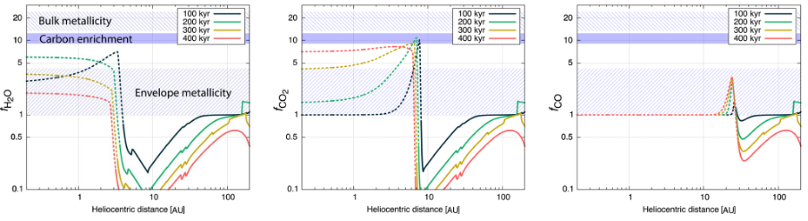
Santiago Triana, Jeremy Rekier, Ankit Barik, Antony Trinh, and Tim Van Hoolst

The gas giant planets in our solar system can sustain global oscillations, i.e. modes, whose frequencies depend on the interior structure of the planet. These oscillations can be excited by the orbiting moons via tidal forces. The energy dissipated in this oscillatory motions can have a profound impact on the orbital evolution of the moons, much in the same way as the energy dissipated in the Earth's oceans makes our moon gradually recede. Thus, it is important to have both a qualitative and quantitative understanding of these global modes and their dependence on the interior structure of the planet. We present an efficient, fully spectral, numerical method to compute these global modes using the anelastic approximation. Here we showcase the possibilities of the code using simple structure models. However, our method is flexible enough to incorporate differential rotation and magnetic effects. We have made our code freely accessible, hoping it can become a useful tool for the planetary science community.

How to cite: Triana, S., Rekier, J., Barik, A., Trinh, A., and Van Hoolst, T.: Kore: an open, fast, and efficient code to compute global eigenmodes in gas giant planets, Europlanet Science Congress 2026, The Hague, The Netherlands, 7–11 Sep 2026, EPSC2026-910, https://doi.org/10.5194/epsc2026-910, 2026.

F3.2
|
EPSC2026-302
|
On-site presentation
Artyom Aguichine, Olivier Mousis, and Robin Canup

Introduction

Saturn exhibits atmospheric volatile enrichments and bulk metallicities exceeding those of Jupiter despite comparable heavy-element masses, implying formation in a chemically distinct region of the protosolar nebula (PSN). Jupiter is increasingly associated with formation near the H2O iceline, where inward drift and recondensation of icy solids generate strong metallicity enhancements. By analogy, Saturn’s enhanced carbon abundance suggests formation farther from the Sun, potentially near the CO2 or CO icelines. 

This study investigates whether Saturn’s atmospheric and interior composition can be reproduced through formation near these icelines. Particular emphasis is placed on the cold-finger effect, in which inward-drifting icy solids sublimate at icelines, producing vapor enhancements that diffuse and partially recondense near condensation fronts. These processes create localized enrichments in solids and vapors that may control giant-planet compositions.

The work also explores broader implications for Solar System formation. If Jupiter formed near the H2O iceline and Saturn near the CO2 iceline, the giant planets would reflect a systematic chemical gradient across the PSN. The study therefore tests whether Saturn’s observed carbon and phosphorus enrichments favor formation near the CO2 iceline over alternative scenarios.

Methodology

The study employs a one-dimensional viscous α-disk model describing the evolution of the PSN. The model tracks the coupled transport of gas, solids, and vapors while computing the radial and temporal evolution of volatile species. Turbulent viscosities range from α = 5×10⁻⁴ to 5×10⁻³.

The chemical inventory includes 13 trace species: H2O, CO, CO2, CH3OH, CH4, N2, NH3, H2S, PH3, Ar, Kr, Xe, which form pure condensates, and refractory dust. These species evolve through advection, diffusion, radial drift, sublimation, and condensation. Icelines are dynamically defined as locations where solid and vapor abundances are equal.

The model assumes protosolar abundances and explores several carbon partitioning scenarios. Fiducial models adopt CO:CO2:CH3OH:CH4 ratios of 10:30:1.67:1, motivated by interstellar and cometary measurements, while additional CO-rich cases test the sensitivity of Saturn’s formation environment.

Disk metallicity profiles, including both solids and vapors, are compared with Saturn’s inferred envelope metallicity and atmospheric enrichments derived from Cassini observations and interior models. The study also includes a simplified pebble-to-planetesimal conversion prescription to evaluate whether regions enriched by the cold-finger effect can efficiently support giant-planet core formation.

Results

The simulations show that strong metallicity enhancements naturally arise at volatile icelines through the cold-finger effect. Among all volatile species, the CO2 iceline produces the most favorable conditions for reproducing Saturn’s composition. In contrast, the CO iceline generates only weak enrichment peaks because vapor diffusion becomes inefficient at large heliocentric distances (see Fig. 1).

Saturn’s envelope metallicity is reproduced only under relatively low turbulence conditions (α ≤ 10−3) and during the early stages of PSN evolution (<0.3 Myr). Under these conditions, inward drift of CO2-rich icy particles and vapor accumulation interior to the CO2 iceline generate carbon and phosphorus enrichments consistent with Saturn’s atmosphere.

The simulations further show that enrichment amplitudes depend strongly on disk turbulence and the initial CO/CO2 ratio. Lower turbulence preserves sharper enrichment peaks, while CO2-dominated volatile inventories produce stronger carbon enhancements than CO-rich disks.

A key result is that the CO iceline never reaches sufficiently high metallicity to reproduce Saturn’s inferred envelope composition, even in CO-rich scenarios. This strongly disfavors Saturn formation near the CO iceline and instead supports formation near the CO2 iceline.

Noble-gas enrichments remain close to protosolar values because Ar, Kr, and Xe diffuse more slowly than major carbon-bearing species. Saturn’s noble-gas abundances therefore become sensitive diagnostics of formation timing and location, highlighting the importance of future in situ measurements.

Additional tests indicate that removing solar irradiation strengthens enrichment peaks by moving icelines inward toward denser disk regions. Under these conditions, the model most successfully reproduces Saturn’s carbon and phosphorus abundances. Finally, planetesimal formationcalculations show that efficient pebble concentration naturally occurs near volatile icelines, particularly near the CO2 iceline, providing favorable conditions for both core formation and volatile enrichment.

Fig 1. Volatile enrichment profiles as a function of heliocentric distance at several stages of disk evolution for the fiducial case (α = 10−3 and CO:CO2 = 10:30). From top to bottom: H2O, CO2, and CO, ordered according to the locations of their icelines. Solid lines indicate regions where the species is predominantly in solid form, while dashed lines indicate vapor-dominated regions. In each panel, the lower shaded, central filled, and upper shaded bands represent Saturn’s envelope metallicity, atmospheric enrichment considering only C and P abundances, and bulk metallicity, respectively. Agreement with Saturn’s atmospheric enrichment occurs where the dashed curves intersect the central band, here only near the CO2 iceline.

Conclusions

This work provides strong evidence that Saturn most likely formed near the CO2 iceline of the protosolar nebula rather than near the CO iceline or interior to the H2O iceline. Saturn’s atmospheric carbon enrichment, phosphorus abundance, and inferred envelope metallicity are naturally reproduced through early formation in a low-turbulence disk with a CO2-rich volatile inventory.

The results support a broader picture in which giant planets formed sequentially at distinct icelines within the PSN, with Jupiter associated with the H2O iceline and Saturn with the CO2 iceline. The study also demonstrates that the cold-finger effect plays a fundamental role in shaping giant-planet volatile inventories by generating localized metallicity enhancements near icelines.

The findings imply that Saturn initiated rapid core accretion very early in PSN evolution, within the first few 105 years after disk formation. Finally, future in situ measurements at Saturn, particularly noble-gas abundances and isotopic ratios, will provide decisive tests of this formation scenario and improve our understanding of the chemical evolution of the early Solar System.

Reference: 

Aguichine, A., Mousis, O., Canup, R.M. Saturn’s formation at the carbon dioxide iceline. The planetary Science Journal, submitted.

How to cite: Aguichine, A., Mousis, O., and Canup, R.: Saturn’s Carbon Enrichment Points to the CO2 Iceline , Europlanet Science Congress 2026, The Hague, The Netherlands, 7–11 Sep 2026, EPSC2026-302, https://doi.org/10.5194/epsc2026-302, 2026.

F3.3
|
EPSC2026-1112
|
ECP
|
On-site presentation
Michelle Colantoni and Patrick Irwin

The Great Red Spot (GRS) is one of the most prominent features observed on Jupiter due to its size and distinctive colour, yet many aspects of this vortex remain poorly understood. Fundamental questions regarding the vertical structure, the chromophores responsible for its colour, the distribution of such chromophores and other aerosols remain unanswered. Laboratory experiments in which ammonia (NH3) and acetylene (C2H2) are photolyzed by ultraviolet radiation (Carlson et al. 2016) may provide a solution for the identity of the chromophore. One study suggested that this chromophore could be responsible for the red colour across the whole disk of Jupiter, giving rise to the idea of a “universal chromophore” (Sromovsky et al. 2017), which may be located at the top of the main tropospheric cloud, resembling a “crème brûlée” structure (Baines et al. 2019). Other studies suggest that, while the universal chromophore could be plausible, it may not be the one caused by the NH3‒C2H2 reaction, instead it would be one with a steeper blue absorption gradient (Braude et al. 2020). Alternatively, some studies propose the presence of two chromophores located in both an upper haze and lower haze layer, with the upper haze chromophore possibly corresponding to that produced by the NH3‒C2H2 reaction (Anguiano‐Arteaga et al. 2021; Anguiano‐Arteaga et al. 2026).

More generally, observations indicate that the top of the GRS is located at a higher altitude than the surrounding cloud deck. Consequently, vertical structure models developed for the rest of Jupiter’s disk may not provide accurate solutions for the vortex itself, where each atmospheric layer may be shifted to higher altitudes. We are analysing observations of the GRS obtained by VLT/MUSE (0.480 – 0.930 µm), Cassini/VIMS (0.884 – 5.122 µm), Juno/JIRAM (2.002 – 5.014 µm), and JWST/NIRSpec (1.660 – 3.170 µm, 2.870 – 5.270 µm), using the radiative transfer model ArchNEMESIS (Alday et al. 2025). The usage of multiple instruments, different geometries and a wide wavelength range aims to better constrain the vertical structure and chromophore distribution of the GRS, as well as those of other vortices of interest on Jupiter.

How to cite: Colantoni, M. and Irwin, P.: Understanding the Great Red Spot of Jupiter, Europlanet Science Congress 2026, The Hague, The Netherlands, 7–11 Sep 2026, EPSC2026-1112, https://doi.org/10.5194/epsc2026-1112, 2026.

F3.4
|
EPSC2026-698
|
Virtual presentation
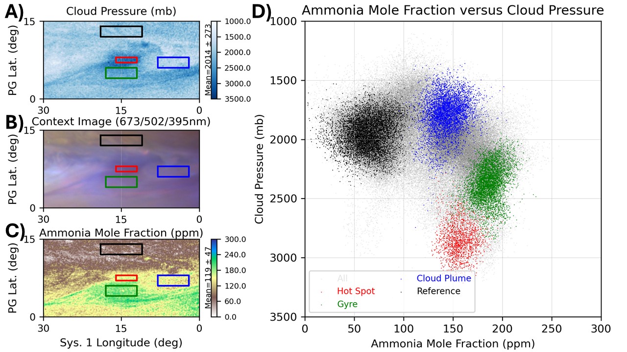
Steven Hill, Leah Tiktin, and Michael Wong

Introduction

Recent observations of Jupiter by HST for the first time used the F645N filter, which is sensitive to ammonia absorption. In combination with the methane sensitive FQ619N filter, both effective cloud-top pressure and ammonia mole fraction can be retrieved using image ratio techniques. Here we present initial results from observations in the last quarter of 2025, focusing on Equatorial Zone (EZ) features. The EZ is important because it exhibits a wide variation in ammonia and cloud structure so that different atmospheric depths and dynamical processes can be probed. The northern EZ exhibits longitudinally periodic features related to a trapped global atmospheric wave there. The wave manifests itself in features including 5µm hot-spots, cloud plumes, and anticyclonic gyres slightly to the south of the other two features. Overall, the EZ is enriched in ammonia, generally more so north of the equator. The North Equatorial Belt (NEB), adjacent to the EZ, is highly depleted in ammonia with little longitudinal variation. Our goals are to 1) Determine whether the measured horizontal spatial variations in ammonia mole fraction represent true physical variations or are simply reflective of measurements of a spatially uniform profile at different cloud pressures and 2) To distinguish the ammonia and cloud properties associated with visually recognizable features and tying them to physical processes. 

Discussion

Using the band-approximation technique we compute the cloud pressure, PCld, and ammonia mole fraction, fNH3, at each mapped latitude and longitude [1, 2]. In addition, we compute the Altitude Opacity Index (AOI, R889/R275) and Color Index (CI, R395/R631) of each location [3]. The spatial sampling of the maps is 0.05° x 0.05°. In addition, we create tricolor images for visual context (RGB: 673, 502, 395 nm) and to locate deeper clouds and higher hazes (RGB: 673,727, 889 nm) [4]. We restrict our analysis to specific groups of features near the sub-observation point and apply an empirical flattening function to the data to mitigate mild limb darkening effects that occur within 30° of the central meridian. 

Two approaches are taken to feature evaluation. First, features of interest are identified by a combination of visual inspection and traditional image and data segmentation techniques. Regions of Interest (ROIs) are generated either by bounding boxes in latitude and longitude drawn around the areas believed to best represent the features or by the raw segmented feature boundaries. Then, clustering analysis is performed graphically and statistically, comparing the samples bounded by the ROIs to each other and to the parent population of the entire mapped area. The ammonia mole fraction and cloud pressure data are visualized in Fig. 1 and show statistically distinct clusters for including 5µm hot-spots, cloud plumes, and anticyclonic gyres. In addition, we look at normalized residuals between fNH3 and PCld to determine where excesses and deficits of ammonia exist beyond what would be expected with a linear relationship between ammonia and cloud pressure. Finally, we look at moving box correlations to see whether within localized areas small-scale variations in cloud pressure yield positive, negative, or neutral correlations with ammonia mole fraction. Finally, we examine color correlations and overlying hazes using the color index and altitude opacity index.

Figure 1. Using HST demonstrates the ability to map cloud-top pressure, PCld, and ammonia mole fraction, fNH3, using high-resolution imaging without full spectra (A, C) while providing visual context (B). The band-approximation method [1] is used (described in the text) and a portion of the northern EZ is shown. Boxed areas highlight feature types related to the EZ planetary wave discussed in the text. D) Scatter plot of PCld versus fNH3 for features shown in Fig. 1 (hot-spot, cloud plume, gyre, and the NEB used as a reference) showing clearly separated clustering. 

Second, an unsupervised Machine Learning (ML) approach using a Gaussian Mixture Model (GMM) is applied to the reflectivity data, the retrieved parameters, and the indices to determine if the human identified regions of interest do or do not correspond to objectively determined clusters in the data. If they do, then this is a strong confirmation of the traditional perception and interpretation of data. If the clustering differs significantly from traditional analysis, this can point to either a weakness in the ML model, or potentially new physics about the relationships between ammonia and cloud pressure for different features. Evaluation of variations in the GMM models and performance with the number of clusters prescribed will be necessary for model optimization. Initial trials with the GMM using just fNH3and PCld show that it seems to identify major features and conditions similar to those identified by a traditional means.

Future Work

Next steps include the improvement of the limb correction for the HST data to address observation time offsets between some of the filter data. We will further develop both the traditional and ML methods and codes so that the full HST data set, including upcoming observations this fall, can be analyzed with a uniform methodology. Finally, we will look for features appearing at multiple viewing angles in the data, which will allow us to use limb darkening to our advantage to explore vertical profiles of aerosols and ammonia.

References

  • Hill, S.M., et al., Spatial Variations of Jovian Tropospheric Ammonia via Ground-Based Imaging. Earth and Space Science, 2024. 11(8): p. e2024EA003562.
  • Irwin, P.G.J., et al., Clouds and Ammonia in the Atmospheres of Jupiter and Saturn Determined From a Band-Depth Analysis of VLT/MUSE Observations. Journal of Geophysical Research: Planets, 2025. 130(1): p. e2024JE008622.
  • Sánchez-Lavega, A., et al., Colors of Jupiter's large anticyclones and the interaction of a Tropical Red Oval with the Great Red Spot in 2008. Journal of Geophysical Research (Planets), 2013. 118: p. 2537-2557.
  • Wong, M.H., et al., Deep Clouds on Jupiter. Remote Sensing, 2023. 15: p. 702.

How to cite: Hill, S., Tiktin, L., and Wong, M.: HST Observations of Jupiter’s Ammonia and Cloud Pressure: Initial Results, Europlanet Science Congress 2026, The Hague, The Netherlands, 7–11 Sep 2026, EPSC2026-698, https://doi.org/10.5194/epsc2026-698, 2026.

F3.5
|
EPSC2026-392
|
On-site presentation
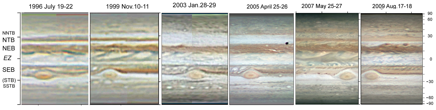
John Rogers

Summary & Introduction

Episodes of reddish or yellowish coloration of the Equatorial Zone (EZ), either in a broad Equatorial Band (EB) or more widely, have been noted throughout observational history [Ref.1].  More recently, a long-term survey at 5 microns by Antuñano et al. [Refs.2,3] has shown episodes of brightening, i.e. cloud clearance in the EZ (‘EZ disturbances’), which partially coincide with coloration episodes, and a periodicity of 6.6 (±0.5) years was proposed though some events were ‘missing’.  Here we review the history of colorations since 1971 from amateur observations, so as to give a systematic account for comparison with the 5-mm data.  This comparison reinforces the evidence for the 7-year period, and shows that this phenomenon has several dissociable aspects.

Reddish coloration and/or darkening was present more often than not in the 1960s and 1970s, but episodes have been more distinct in other decades.  From the 1990s onwards they are well documented by colour and colour-filter imaging, which gives objective data even though our descriptions are still largely subjective.  While some episodes exhibit obvious yellow or orange or duller ochre colour, and can last for several years, other episodes show only a brownish-grey shade changing to neutral dark grey, and only last for 1-2 years.  Some episodes begin with a pure yellow or orange colour, which then becomes darker and less saturated [Ref.1].  

Coloration episodes since 1971

Episodes up to 1991 were described in [Ref.1]. Subsequent episodes were described in the interim reports of the BAA Jupiter Section [https://britastro.org/sections/jupiter]. Figs.1 & 2 show examples of maps from amateur images, mostly made by M. Vedovato and R. Bullen. In the following description, 5-micron information after 1979 is from [Refs.2-4].

1972-76: Pure yellow-orange colour during 1972, which then condensed into a massive dark brown or grey-brown EB including southern EZ while the SEB was whitened (1973-1975).  It was grey in 1976, then faded away. (This massive belt was also 5-micron-bright from 1973-1976: Ref.5.)

1977-82: Largely pure colour, strong yellow or ochre over most of EZ, but with grey EB component in 1978-79 and thereafter; then, yellow colour gradually retreating to EZ(S) and fading. (It was 5-micron-bright in 1979 [Ref.5]; no data in other years.)

(1986: Although NEDFs and grey shadings were prominent, the EZ remained largely white so there was no coloration event. There was also no 5-micron event, pausing the 7-year periodicity.)

1989-1992: Started as pure yellow colour in late 1989, becoming brown or (eventually) grey in 1990-92, with the colour shifting southwards. (5 micron coverage was not continuous, but EZ was still dark until 1991 May, then bright in 1992 Jan-April.)

1999-2000:  A brown EB developed in mid-1999, then became dark grey from 1999 Nov. to 2000 Jan. (At 5 microns, similar timecourse.)

2006-2007:  In 2006, dark features accumulated all across the EZ including a brown EB. In 2007, the whole EZ was largely grey-brown. It faded after July but brown EB was still present at some longitudes up to 2008 May.  (At 5 microns, similar timecourse.)

2012-2013:  Orange colour in an EB from 2012 June to 2013 March, particularly in 2012 July-August, coinciding with the vigorous revivals of the NTB and NEB.  Weak at some longitudes, and not methane-bright.

2018-2022:  Orange colour developed gradually in 2018 (March-May), and was intense in late 2018 and in 2019.  It was fainter in early 2020 but revived in late 2020, and was intense during 2021.  It faded away in the second quarter of 2022. (There was a weak 5-micron-bright EB in 2019 Jan., but otherwise only small weakly 5-micron-bright streaks from 2018 Aug. (not earlier) to 2021 [Ref.4; G. Orton et al., EPSC2022-761; G. Orton, pers.com.].)

Stationary features in orange haze over EZ:  During much of this episode, the orange EB was particularly bright in methane-band images, and we detected waves on its S edge (in 2020) and large methane-bright patches (in 2021) that were almost stationary in System III [J.Rogers & C.Go, EPSC2021-95]. This is unprecedented, and suggests that the orange, methane-bright haze extended up to very high altitude. 

2024-2025: A grey-brown EB gradually appeared from 2023 Dec. onwards, and was notable in 2024-25; it faded away in 2025 Dec.  (There was a partial 5-micron-bright EB for much of this time: G. Orton, pers.com.)

Relation to 5-micron clearances

These coloration episodes fit the cycle of ‘EZ disturbances’ with period of 6-7 years proposed in [Refs.2,3] on the basis of brightening in the thermal infrared at 5 microns.  Neither these, nor visible reddish coloration, alone reveal a clear periodicity.  But if we combine the record of dark brownish-grey episodes, orange or ochre episodes, and 5-mm clearances, the 6-7-year periodicity is consistent (Fig.3):

_____________________________________________________________________________________________________

The brown/grey episodes have lasted less than 2 years, coinciding with the 5-micron clearances, and are simply understood as substantial clearance of the main cloud deck producing both the low albedo and the bright thermal signal. The more vividly coloured episodes are more complex, and sometimes last for several years while the 5-micron clearance is much shorter or even (in 2012) does not occur at all.  The orange coloration must be an additional aerosol, which Antuñano et al.[Ref.4] suggested was exposed by the removal of the upper clouds. Indeed it is not always methane-bright (e.g. 2012), but sometimes it is (1972; 2020-21), indicating higher altitude.  The temporal coincidence and periodicity of these events imply that they are all part of one complex phenomenon, which can entail cloud clearance and/or orange aerosol formation in different proportions. 

References:

  • [1]  Rogers JH (1995) The Giant Planet Jupiter  (Cambridge Univ. Press).
  • [2]  Antuñano A et al.(2018). Geophysical Research Letters 45, 10987-95.    https://doi.org/10.1029/2018GL080382.
  • [3]  Antuñano A et al. (2019) . Astronomical Journal 158, no. 130.   https://iopscience.iop.org/article/10.3847/1538-3881/ab2cd6
  • [4]  Antuñano A et al. (2020). JGR-Planets, 125, e2020JE006413.  https:// doi.org/10.1029/2020JE006413
  • [5]  Terrile RJ & Beebe RF (1979) Science 204, 948-951.

I thank Glenn Orton for information about recent 5-micron clearances.

How to cite: Rogers, J.: Jupiter’s Equatorial Zone:  Visible colorations and 5-micron clearances together support 7-year periodicity, Europlanet Science Congress 2026, The Hague, The Netherlands, 7–11 Sep 2026, EPSC2026-392, https://doi.org/10.5194/epsc2026-392, 2026.

F3.6
|
EPSC2026-710
|
ECP
|
On-site presentation
Shawn Brueshaber, John Rogers, Isabel Williams, Gerald Eichstaedt, Glenn Orton, and Candice Hansen

Jupiter’s north pole is attended by eight circumpolar cyclones (CPCs) surrounding a central North Polar Cyclone (NPC) [Fig.1].  They were discovered by the JunoCam and JIRAM instruments on Juno (Ref.1), and have been remarkably stable ever since.  Here we use JunoCam maps to track the positions of the CPCs and NPC throughout the Juno mission, as well as the behaviour of several ancillary circulations which have persisted for some time.  CPC-7 is always further from the pole than the others, and the NPC is always offset into one quadrant by up to 1.2° from the pole.
Circumpolar cyclones
Here we track longitudes of the 8 CPCs up to perijove (“PJ”) 73 [Fig.2], extending the analysis of Ref.2.  The CPCs have only shown modest changes on longitude.  The results show that the octagon moves largely as a whole, with trends on a timescale of several months to a year. 
Most of the CPCs decreased slightly in longitude up to PJ8 then increased between PJ12 and PJ17, as already shown in Ref.2. The CPCs have been generally stationary since then, except between PJ31 and PJ42, when they all increased in longitude substantially then decreased again, though remaining several degrees higher than before.  This positive excursion peaked between PJ35 and PJ38, not quite synchronously for all the CPCs, with an increase of 8°-18° relative to their overall mean motion; all other deviations from the mean motion were smaller. Since then, they have all been essentially stationary since then apart from CPC-7 and CPC-6.  Overall, the CPCs longitudes have increased by an average of 16 (±5) deg in 9.0 years, but variations are neither progressive nor cyclic.
These results show that the north polar octagon does not copy the systematic rotation and  precessional motion of the south polar pentagon (Refs.2, 4, 5), which have been reproduced in a model by Gavriel & Kaspi (Ref.6). However, the lag between longitude changes of CPCs suggests that similar interactions between adjacent cyclones may occur. 
We also briefly detail the varying morphologies of each of the CPCs, noting that they tend to fall into either a ‘filled’ category or a more diverse category including spiral and chaotic forms.  The ‘filled’ CPCs have mostly grown larger during Juno’s mission, especially CPC-1.  Only CPC-5 has not grown.  This may suggest a seasonal change, although any reversion to smaller size would have to occur rapidly during the so-far-unobserved portion of the jovian year. 
The NPC itself, while appearing as a spiral form, and consistently so, is quite different from the others in radio wavelengths (see other presentations this conference). 

Extra circulations
While the 8 CPCs and the NPC are the only features that have persisted throughout Juno’s mission, several other circulations in and around the octagon have been followed for multiple perijoves.
Anticyclonic white ovals (AWOs) inside the octagon:  There are always one or two AWOs inside the octagon. One is usually present poleward of CPC-7 (except PJ32 to PJ39) [Fig. 1: PJ57/58 map]; the other (b) was seen from PJ25 to PJ55, poleward of CPCs-3/4/5, though swinging unpredictably in longitude.  It seems likely that the two merged just after PJ57, creating an AWO poleward of CPC-1 from PJ62 to PJ70, while a new vortex developed poleward of CPC-7.
AWO just outside the octagon:  A large AWO was tracked from PJ47 to PJ70. [Fig.3. PJ43-PJ70]. After eddying in a small clockwise loop from PJ43 to PJ47, from PJ47 to PJ51 it drifted anticlockwise around the periphery of the octagon at 79.5 (±0.14)°N, consistent with the outer winds of the CPCs. Then at PJ52 it had probably merged with a smaller AWO, and almost stopped moving.  From PJ53 to PJ64 it remained just S of CPC-1&2, again oscillating slightly in clockwise loops. At PJ64 it apparently broke loose from this eddy and moved to a lower latitude, then from PJ67 to PJ70 it drifted clockwise (retrograde) around the octagon at 78.0—79.0°N.  
Ancillary cyclones:  Sometimes one or two extra cyclones are seen at corners of the octagon, resembling smaller versions of filled CPCs, added to the vortex crystal.  Two lasted for some time.  One, labelled ‘X’, was recorded from PJ30 to PJ45 [Fig 5]. At PJ50, it was either absent or reduced, but a small cyclone from PJ58 to PJ66 may qualify as a revival of ‘X’.  The other ancillary cyclone is labelled ‘IX’ [Fig 4. PJ32-PJ39]. At PJ32 & PJ33 it was a small version of a ‘filled’ CPC. At PJ36 to PJ39, if this was the same object, it had a similar cloud texture but an elongated, distorted outline, and it was drifting clockwise (retrograde) around the octagon at 77.6—78.7°N.  
These drifts, for the cyclone and the AWO, did not exceed 2.1 m/s, and were usually < 1 m/s -- much slower than the wind speeds in CPCs or jets.  They are consistent with the flow patterns that we found around the south polar polygon: AWOs with variable prograding drift adjacent to the CPCs [Ref.2], and a zone slightly further out in which the average drift was weakly retrograding [Ref.3].
Acknowledgements:  
We thank Michael Ravine and Michael Caplinger (Malin Space Science Systems) and Tom Momary (formerly JPL) for enabling the operation of JunoCam.  Some of this research was funded by NASA, in part through JPL/CalTech. 
References:
1.   Adriani A et al. (2018),  Nature 555, 216-219. 
2.  Tabataba-Vakili F et al.(2019/20),  Icarus 335, paper 113405. https://doi.org/10.1016/j.icarus.2019.113405
3.  Rogers J et al. (2021/22),  Icarus 372, paper 114742. https://doi.org/10.1016/j.icarus.2021.114742
4.  Rogers J et al. (2021), EPSC Abstracts Vol. 15, EPSC2021-57, 2021. https://doi.org/10.5194/epsc2021-57
5. Mura A et al. (2021), GRL 48, e2021GL094235. https://doi.org/10.1029/2021gl094235
6. Gavriel N & Kaspi Y (2022), GRL 49, e2022GL098708. https://doi.org/10.1029/2022GL098708


How to cite: Brueshaber, S., Rogers, J., Williams, I., Eichstaedt, G., Orton, G., and Hansen, C.: Tracking Jupiter’s North Polar Vortices from JunoCam, Europlanet Science Congress 2026, The Hague, The Netherlands, 7–11 Sep 2026, EPSC2026-710, https://doi.org/10.5194/epsc2026-710, 2026.

F3.7
|
EPSC2026-769
|
On-site presentation
Glenn Orton, Kevin Kelly, Kiara Donolo, Gerald Eichstaedt, and Shawn Brueshaber

Abstract. The JunoCam instrument on the Juno mission has been used to detect and measure properties of detached haze layers in Jupiter’s atmosphere using observations of the planet’s limb. Although results are preliminary, a surprising concentration of detached haze layers was found in a discrete planetocentric latitude range of 30°-35°N, well separated from prominent hazes associated with the north polar region.

Introduction. The JunoCam instrument on the Juno spacecraft has sufficient spatial resolution to characterize haze properties using observations that resolve vertical distribution of haze particles at the limb. Some of these observations reveal the presence of detached hazes. These hazes may influence Jupiter’s atmospheric dynamics, radiative balance and photochemistry, and we have studied their presence or absence at each latitude in an effort to constrain meridional variability in atmospheric processes. This effort required sorting through considerable complexities such as the changing observational geometry, to derive the frequency and distribution of these hazes. Observational circumstances such as resolution, exposure, solar incidence angle and phase angle differ substantially and those difference affect the visibility of these faint atmospheric hazes, contributing to observational biases and non-detections.

The Juno spacecraft repeatedly observed Jupiter in limb-viewing geometry with JunoCam providing higher-resolution images across many close approaches, known as perijoves. These close-up images contain valuable information about vertical atmospheric structure and interpreting these observations consistently required the systematic handling of cases where the limb boundary is not sharply defined. A programmatic pipeline was developed to process JunoCam images and sort them into three categories: detection, non-detection, or ambiguous.

Methods. By analyzing the changing peaks in image brightness (Figure 1), this framework allows for the systematic classification of individual image sets, enabling the consistent comparison of detached haze detection across latitudes. Strict geometric and detectability filters were applied so that retained detections represent only cases where detached haze is clearly resolvable above instrumental and viewing limitations. As a result, the occurrence statistics we derived should be interpreted as robust but likely incomplete, emphasizing reliability over sensitivity. Figure 2 illustrates the accumulated counts from all images in PJ14.

Figure 1. Brightness profiles illustrating primary and secondary peaks used in deteched-haze classifications. The image on the left panel illustrates a non-detection of a detached haze, and the right panel illustrates the detection of a detached haze.

Figure 2. Detached haze detection frequency at various latitudes derived from limb classifications using the validated pipeline. The peak at planetocentric 30°-35°N is a robust feature that appears in several images. The “picket-fence” appearance at high latitudes is the result of sparse coverage, where only a few geometry-valid limb fragments contribute, so individual detections produce isolated spikes.

Results. The present results are preliminary and are based primarily on PJ14, with additional methodological refinements and analysis of earlier southern perijoves still in progress and to be discussed in this presentation. 

Figure 3 expands the results of Figure 2, showing the detached-haze signal on an image-by-image basis for all images in PJ14, highlighting its confinement to a narrow mid-latitude band (~30–35°) over several longitudes, and makes clear that the analysis is intentionally conservative through the detectability masking. In favorable observations, the separation between the two maxima in the radial brightness gradient corresponds to an apparent detached haze altitude of approximately 70–80 km above the main cloud deck, roughly three atmospheric scale heights. This may actually be an under-estimate of the distance to the main cloud top, since, in general, there might exist an additional haze layer above the main cloud top that is only obvious in the limb perspective, and hence reduces the apparent altitude of the detached haze layer above the main cloud deck.

Figure 3. Figure 3. Longitude–latitude occurrence map for detached haze during Perijove 14. Colors indicate the fraction of detectably valid fragments exhibiting secondary peaks within each longitude–latitude cell; cells below the minimum fragment threshold are masked. The mid-latitude enhancement is retained in map space but remains coverage-limited in longitude under the limited range of JunoCam’s viewing geometry in PJ14.

This result is surprising, prompting us to double-check it by examining the raw images, which verified its presence.  This is well south of the upper-atmospheric hazes apparent in the northern polar hood. It may provide a clue about the formation of those hazes.  It could simply be a diluted extension of the north polar hood that drifted southward. Alternatively, it is a radiation-induced haze that is produced at a slower rate than the polar hazes caused by energetic radiation interacting with the upper atmosphere. Additional clarity will ensue from our extension of this study to greater latitude ranges, including not only the north but also a hemispherical cross-comparison with several measurements made early in the mission at southern latitudes. Comparisons will be made with other Juno measurements, as well as historical observations (Rages et al 1998).

Acknowledgements. Some of this research was carried out at the Jet Propulsion Laboratory, California Institute of Technology, under a contract with the National Aeronautics and Space Administration (80NM0018D0004). KK was an intern at JPL in the Student Independent Research Internship (SIRI) program during part of this work. KD was a Caltech Summer Undergraduate Research Fellow (SURF) at JPL during this work.

All analyses were performed using an open-source, fully reproducible pipeline. 

Dedication. We dedicate this work to the memory of Dr. Candice Hansen, who was the Juno instrument lead for JunoCam through most of the mission.  She provided operational insight  and guidance for both the public access to Juno observations envisioned for this instrument and for the strong quantitative scientific results it brought to the mission.

Reference:

K. Rages, R. Beebe, D. Senske. 1998. Jovian stratospheric hazes: The high phase angle view from Galileo. Icarus 139, 211-226;


How to cite: Orton, G., Kelly, K., Donolo, K., Eichstaedt, G., and Brueshaber, S.: Preliminary Assessment of Detached and Other Hazes in Jupiter’s Atmosphere from JunoCam Observations, Europlanet Science Congress 2026, The Hague, The Netherlands, 7–11 Sep 2026, EPSC2026-769, https://doi.org/10.5194/epsc2026-769, 2026.

F3.8
|
EPSC2026-991
|
ECP
|
On-site presentation
Joseba Ullibarri-Lombraña, Peio Iñurrigarro, Naiara Barrado-Izagirre, Agustín Sánchez-Lavega, and Santiago Pérez-Hoyos

The Juno mission, in orbit around Jupiter since July 2016, has provided an unprecedented view of the planet’s atmospheric dynamics. High-resolution images from the JunoCam camera aboard Juno have led to the identification of small-scale compact cloud formations known as pop-up clouds [1], which appear as elevated features projecting shadows over their surrounding clouds. These features are distinguished from large-scale strong convective outbreaks by their smaller spatial and vertical scales [2, 3], suggesting they are powered by the less vigorous ammonia moist convection [4]. A compact cluster of clouds of this type was also observed within the Great Red Spot in the very high-resolution images from JunoCam [5]. While deep convective phenomena can have large vertical extents reaching altitudes of a few tens of kilometers above the main cloud deck [6], recent studies suggest that pop-up clouds rise to around 15 km above their immediate surroundings [4].

In this work, we used JunoCam high-resolution images to conduct a morphological classification of these small-scale moist convection pop-up clouds across a wide range of latitudes and dynamical environments, including Folded Filamentary Regions (FFRs), vortex interiors, vortex peripheries, and others. In addition, we performed a comprehensive morphological characterization of these features, employing a Geographic Information System (GIS) framework [7] with a geodetic metric, based on an oblate spheroid model defined by Jupiter’s radius and flattening parameter. Our results show that pop-up clouds are present across all latitudes covered by JunoCam and exhibit significant spatial clustering. The morphological classification highlights a variety of shapes, from compact cells and cloud-clusterings to elongated filaments. Measurements reveal varying horizontal scales but consistent separations within individual clusters. Furthermore, we also studied vertical elevations derived from projected shadows, which remained below 15 km above the surrounding cloud deck.


References

[1] Hansen et al. (2019). JunoCam Images of Castellanus Clouds on Jupiter. AGU Fall Meeting Abstracts, 2019, P44A-05. https://ui.adsabs.harvard.edu/abs/2019AGUFM.P44A..05H


[2] Orton et al. (2022). Investigating Relative Cloud Heights in Jupiter Using Juno's JunoCam Imager. AAS/Division for Planetary Sciences Meeting Abstracts #54, 54, 306.06. https://ui.adsabs.harvard.edu/abs/2022DPS....5430606O


[3] Guillot et al. (2024). How high are Jupiter's clouds? From high-resolution JunoCam images to a multi-wavelength analysis. EGU24. doi:10.5194/egusphere-egu24-17351


[4] Palotai et al. (2023). Moist convection in the giant planet atmospheres. Remote Sensing, 15, 219. doi:10.3390/rs15010219


[5] Sánchez-Lavega A. et al. (2018), The rich dynamics of Jupiter’s Great Red Spot from JunoCam – Juno images, Astronomical J., 156, 162 (9pp), doi:10.3847/1538-3881/aada81


[6] Sánchez-Lavega et al. (2008). Depth of a strong jovian jet from a planetary-scale disturbance driven by storms. Nature, 451 (7177), 437–440. doi:10.1038/nature06533


[7] Trent M. Hare, Angelo P. Rossi, Alessandro Frigeri, Chiara Marmo. Interoperability in planetary research for geospatial data analysis, Planetary and Space Science, Volume 150, 2018, ISSN 0032-0633, https://doi.org/10.1016/j.pss.2017.04.004

How to cite: Ullibarri-Lombraña, J., Iñurrigarro, P., Barrado-Izagirre, N., Sánchez-Lavega, A., and Pérez-Hoyos, S.: Morphological analysis of Jupiter’s small-scale pop-up clouds, Europlanet Science Congress 2026, The Hague, The Netherlands, 7–11 Sep 2026, EPSC2026-991, https://doi.org/10.5194/epsc2026-991, 2026.

F3.9
|
EPSC2026-16
|
ECP
|
On-site presentation
Neil Lewis

Juno has revealed long-lived clusters of circumpolar cyclones (CPCs) in Jupiter's polar regions. These observations were not predicted, challenging our basic understanding of fluid dynamics, and evade simulation by global numerical models, preventing us from testing theories for their existence. 

Global, three-dimensional weather layer General Circulation Models (GCMs) of Jupiter's atmosphere are useful tools for bridging theory and observations. However, they fail to produce CPCs. Two potential causes for this are: (1) low spatial resolution, which precludes GCMs from representing thin, anti-cyclonic 'shields', that are believed to be important for CPC formation; and (2) poor representation of interior-weather layer interaction, which may be important for generating the CPCs. The aim of my research is to design a new Jupiter GCM that is capable of simulating small-scale meteorological features in the polar regions. 

The new model has been constructed using FV3, an open-source finite-volume 'dynamical core' (fluid dynamics solver) developed by the NOAA Geophysical Fluid Dynamics Laboratory (GFDL). FV3 solves the fully-compressible Euler equations for a shallow atmosphere (appropriate for the weather layer) using a cubed-sphere horizontal grid and a Lagrangian, flow-following coordinate in the vertical. FV3 offers several advantages for the simulation of Jovian (and giant planet) atmospheric dynamics. FV3 can be run in a standard 'global-only' configuration, but also has functionality to embed high-resolution regional grids ('nests') within a global GCM. This capability will enable its use for conducting high-fidelity simulation of the Jupiter’s polar regions, overcoming issue (1) above. In addition, FV3 was designed for operational weather forecasting, and is thus designed to be extremely computationally efficient while preserving solution accuracy. Finally, the importance of vorticity dynamics is emphasised in FV3's design, and its advection scheme has the property that the shallow-water potential vorticity (PV) and the helicity are advected as scalars. This allows FV3 to excel in the simulation of cyclones on Earth, and is a major advantage for this research project.

Here, I report results from global-only benchmarking simulations run using this model. Specifically, FV3 has been adapted to incorporate the 'physics packages' (e.g., convective adjustment, radiative transfer) implemented by Schneider and Liu (SL; 2009) and Young et al. (2019) to study Jupiter. Diagnostics obtained from FV3 using these configurations, including: the circulation morphology; the zonal-mean structure of the temperature and zonal wind; eddy statistics; and energy spectra; will be compared against the original results reported in these studies. The aim of this comparison is to quantify the impact of dynamical-core choice on the simulated atmospheric circulation (SL use the GFDL pseudospectral dynamical core, and Young et al. use the MITgcm on an Arakawa-C grid). Provisional results using a nested-grid set-up (with high-resolution grids included at the poles) may also be presented, dependent on the progress of model development between now (April 2026) and EPSC! Future development of the model will focus on adding a stochastic element to the lower-boundary interior heat flux, as an initial step towards overcoming issue (2) above.

References: 1. Schneider and Liu, 2009. J. Atmos. Sci., 66, 3, pp. 579-601. 2. Young, Read, and Wang, 2019. Icarus, 326, pp. 225-252.

How to cite: Lewis, N.: A New Model for Jovian Weather Layer Dynamics, Europlanet Science Congress 2026, The Hague, The Netherlands, 7–11 Sep 2026, EPSC2026-16, https://doi.org/10.5194/epsc2026-16, 2026.

F3.10
|
EPSC2026-245
|
On-site presentation
Ngan H. D. Trinh, Sandrine Guerlet, Jérémy Leconte, Aymeric Spiga, Noé Clément, Ehouarn Millour, and Enora Moisan

Jupiter's turbulent atmosphere is host to intense convective and storm activity. These phenomena range from towering small-scale plumes reaching 50 km in height to massive mesoscale complexes spanning thousands of kilometers (Palotai et al., 2023). Often accompanied by lightning, these storms are mainly powered by the latent heat released from water condensation and are triggered by the planet's internal heat flux (Ingersoll et al., 2000; Palotai et al., 2023) and/or local dynamics (Sankar et al., 2025). Understanding the mechanisms that trigger and shape these convective events has motivated the development of various Cloud-Resolving Models (CRMs) (Hueso & Sánchez-Lavega, 2001; Sugiyama et al., 2014; Li & Chen, 2019). Continuing to improve these models is crucial for interpreting current observations from the Juno spacecraft (Fletcher et al., 2020; Read, 2024) and preparing for the upcoming JUICE mission.

To gain insight into Jupiter's deep moist convection, we utilize a 3D Cloud Resolving Model (CRM). The non-hydrostatic dynamical core of the model is inherited from the terrestrial Weather Research and Forecasting (WRF) model. It has been coupled to the physics of the Planetary Climate Model (PCM) suite for various planetary atmospheres, including Mars, Venus, Titan, the Ice Giants (Clément et al., 2024) and temperate exoplanets (Leconte et al., 2024). For Jupiter, our model covers a localized domain of a few hundred kilometers at a high spatial resolution (~1-2 km in both horizontal and vertical dimensions), allowing us to explicitly resolve individual small-scale convective plumes. For initial conditions, we first run a 1D radiative-convective version of the model (Guerlet et al., 2020) until a steady state is reached (after ~25 Jovian years). The resulting temperature, pressure, and humidity profiles are then utilized as the background atmospheric sounding to initialize the 3D simulations (Clément et al., 2024). Note that we currently include the condensation/precipitation/evaporation of water only, and not the other condensates.

We conduct benchmarking tests to validate the model's performance under Jovian conditions. This includes evaluating the sensitivity of the model to various grid configurations (such as vertical resolution and model top placement) to mitigate numerical artifacts and ensure dynamic stability. Preliminary 3D simulations successfully showcase the spontaneous formation of water storms driven by latent heat release of water.  We report the development of distinct convective structures, characterized by strong, localized updrafts (reaching vertical velocities on the order of ~50-100 m/s) and precipitation-driven downdrafts.

Following the finalization of the benchmark test cases, this CRM is planned to be used to systematically investigate the influence of varying atmospheric forcing on storm properties. We will explore how different internal heat fluxes, insolation levels, and deep-water abundances affect the horizontal and vertical extent, intensity, frequency, and lifetime of convective plumes. Ultimately, this local-scale modeling will serve as a stepping stone for future regional-scale studies, helping to parameterize the effect of small-scale storms on Jupiter's large-scale circulation and alternating zonal winds in Global Circulation Models (GCMs).


References

Clément, N., et al. (2024). Storms and convection on Uranus and Neptune: Impact of methane abundance revealed by a 3D cloud-resolving model. Astronomy & Astrophysics, 690, A227. https://doi.org/10.1051/0004-6361/202348936

Fletcher, L. N., et al. (2020). How well do we understand the belt/zone circulation of giant planet atmospheres?. Space Science Reviews, 216(2), 30. https://doi.org/10.1007/s11214-019-0631-9

Guerlet, S., et al. (2020). Radiative-equilibrium model of Jupiter’s atmosphere and application to estimating stratospheric circulations. Icarus, 351, 113935. https://doi.org/10.1016/j.icarus.2020.113935

Hueso, R., & Sánchez-Lavega, A. (2001). A three-dimensional model of moist convection for the giant planets: The Jupiter case. Icarus, 151(2), 257-274. https://doi.org/10.1006/icar.2000.6606

Ingersoll, A. P., et al. (2000). Moist convection as an energy source for the large-scale motions in Jupiter's atmosphere. Nature, 403(6770), 630-632. https://doi.org/10.1038/35001021

Leconte, J.,  et al. (2024). A 3D picture of moist-convection inhibition in hydrogen-rich atmospheres: Implications for K2-18 b. Astronomy & Astrophysics, 686, A131. https://doi.org/10.1051/0004-6361/202348928

Li, C., & Chen, X. (2019). Simulating Nonhydrostatic Atmospheres on Planets (SNAP): Formulation, Validation, and Application to the Jovian Atmosphere. The Astrophysical Journal Supplement Series, 240(2), 37. https://doi.org/10.3847/1538-4365/aafdaa

Palotai, C., et al. (2023). Moist Convection in the Giant Planet Atmospheres. Remote Sensing, 15(1), 219. https://doi.org/10.3390/rs15010219

Sankar, R., et al. (2025). Wind Shear and the Role of Eddy Vapor Transport in Driving Water Convection on Jupiter. The Planetary Science Journal, 6(5), 109. https://doi.org/10.3847/PSJ/adcc21

Read, P. L. (2024). The Dynamics of Jupiter’s and Saturn’s Weather Layers: A Synthesis After Cassini and Juno. Annual Review of Fluid Mechanics, 56, 271-293. https://doi.org/10.1146/annurev-fluid-121021-040058

How to cite: Trinh, N. H. D., Guerlet, S., Leconte, J., Spiga, A., Clément, N., Millour, E., and Moisan, E.: Modeling Jupiter’s Convective Plumes: First Results from a High-Resolution 3D Cloud-Resolving Model, Europlanet Science Congress 2026, The Hague, The Netherlands, 7–11 Sep 2026, EPSC2026-245, https://doi.org/10.5194/epsc2026-245, 2026.

F3.11
|
EPSC2026-437
|
ECP
|
On-site presentation
Paula Avalle-Gràcia, Ricardo Hueso, and Peio Iñurrigarro

Water is thought to play a crucial role in the formation and evolution of Jupiter and Saturn. At the same time, water is also a key element in shaping various phenomena in the weather layers of these planets. For example, large and intense convective storms in Jupiter are interpreted as the signature of intense water moist convection driven by the release of latent heat when water condenses. The largest convective storms in Jupiter suggest a minimum water abundance of at least 1 times solar, and possibly higher [1]. However, in Gas Giants atmospheres, where dry air is composed of hydrogen and helium, water increases the molecular weight of a parcel and can completely inhibit moist convection for water abundances on the order of 5 times solar [2, 3]. Juno measurements with the MWR instrument suggest a deep-water abundance of 2.7 ± 2.0 [4] with the highest possible values near the convective inhibition limit. Thus, a relevant question raised by Juno measurements is what are the potential characteristics of water powered moist convective storms close to the convective inhibition limit.

Here, we use a three-dimensional cloud-resolving model [5] with highly parametrized microphysics to simulate water driven moist convective storms examining different water abundances close to the convective inhibition limit around 5 times solar abundance. We find that weak perturbations are able to start moist convection when water abundance is low, but strong perturbations are still able to trigger intense convective storms near the limit of inhibition. Our results represent a first step toward the development of a new generation of convective models aimed at addressing open questions about atmospheric dynamics in Gas Giant planets, particularly in the context of the upcoming JUICE mission.


References

[1] Sánchez-Lavega, A. et al. 2008, Nature, 451, 437-440

[2] Guillot, T. 1995, Science, 269, 1697

[3] Leconte, J. et al. 2017, A&A, 598, A98

[4] Li, C. et al. 2020, Nature Astronomy, 4, 609-616

[5] Hueso, R. & Sánchez-Lavega, A. 2004, Icarus, 172, 255-271

How to cite: Avalle-Gràcia, P., Hueso, R., and Iñurrigarro, P.: Three-dimensional simulations of moist convective water storms in Jupiter’s atmosphere: exploring the dichotomy between energetic storms and the inhibition of convection, Europlanet Science Congress 2026, The Hague, The Netherlands, 7–11 Sep 2026, EPSC2026-437, https://doi.org/10.5194/epsc2026-437, 2026.

F3.12
|
EPSC2026-614
|
ECP
|
On-site presentation
Aida Flix-Bellmunt, Agustín Sánchez-Lavega, Enrique García-Melendo, Arnau Miró, and Manel Soria

The AV is an anticyclonic vortex on Saturn that formed at approximately 40°N following the Great White Spot (GWS) of 2010 and has remained active since then. During its first year, the vortex migrated northward to 44°N and then returned to 43°N, where it has since exhibited latitudinal oscillations (Hueso et al., 2020). This migration is theoretically attributed to the β-drift effect, which is driven by vorticity gradients and controlled by the barotropic beta parameter (βb), i.e., the sum of the relative and planetary vorticity gradients. For anticyclones, a poleward migration occurs when βb < 0, while the vortex moves equatorward when βb > 0. Analyzing the zonal wind profiles retrieved with Cassini during 2004—2009 (García-Melendo et al., 2011), Trammell et al. (2016) calculated the relative vorticity and presented a latitudinal profile. From it, they found that the AV formed at a region where βb < 0 and identified 43°N as an equilibrium point (βb = 0). In this study, we employed a Shallow Water model to simulate the positional evolution of the AV after its formation for 100—150 days, limited by numerical dissipation. We retrieved the northward drift rate and compared it to the observed 2011 migration rate (Hueso et al., 2020). The simulations provide further insight into the influence of the zonal wind profile shape on vortex drifting. Furthermore, the retrieved migration velocity serves as a validation benchmark for the numerical model.

References

García-Melendo, E., Pérez-Hoyos, S., Sánchez-Lavega, A., & Hueso, R. (2011). Saturn’s zonal wind profile in 2004–2009 from Cassini ISS images and its long-term variability. Icarus, 215(1), 62–74. https://doi.org/10.1016/j.icarus.2011.07.005

Hueso, R., Sánchez-Lavega, A., Rojas, J. F., Simon, A. A., Barry, T., del Río-Gaztelurrutia, T., Antuñano, A., Sayanagi, K. M., Delcroix, M., Fletcher, L. N., García-Melendo, E., Pérez-Hoyos, S., Blalock, J., Colas, F., Gómez-Forrellad, J. M., Gunnarson, J. L., Peach, D., & Wong, M. H. (2020). Saturn atmospheric dynamics one year after Cassini: Long-lived features and time variations in the drift of the Hexagon. Icarus, 336, 113429. https://doi.org/10.1016/j.icarus.2019.113429

Trammell, H. J., Li, L., Jiang, X., Pan, Y., Smith, M. A., Bering III, E. A., Hörst, S. M., Vasavada, A. R., Ingersoll, A. P., Janssen, M. A., West, R. A., Porco, C. C., Li, C., Simon, A. A., & Baines, K. H. (2016). Vortices in Saturn's Northern Hemisphere (2008–2015) observed by Cassini ISS. Journal of Geophysical Research: Planets, 121(9), 1814–1826. https://doi.org/10.1002/2016JE005122

How to cite: Flix-Bellmunt, A., Sánchez-Lavega, A., García-Melendo, E., Miró, A., and Soria, M.: Shallow Water Simulations of the Latitudinal Drift of Saturn’s Anticyclonic Vortex (AV), Europlanet Science Congress 2026, The Hague, The Netherlands, 7–11 Sep 2026, EPSC2026-614, https://doi.org/10.5194/epsc2026-614, 2026.

F3.13
|
EPSC2026-933
|
ECP
|
On-site presentation
Simon Toogood, Leigh Fletcher, Oliver King, Michael Roman, Imke de Pater, Francesco Biagiotti, Henrik Melin, Thierry Fouchet, Mike Wong, and Pablo Rodriguez-Ovalle

We present observations of Jupiter’s south polar region using the JWST/NIRSpec IFU spectrometer, providing high resolution spectral imaging across the near-infrared that probes the vertical and latitudinal distribution of aerosols and gaseous species.  Near-infrared spectroscopic mapping is a powerful diagnostic for studying giant planet atmospheres, enabling constraints on cloud structure in the weather-forming lower troposphere, and haze in the radiatively-controlled lower stratosphere.  The 1.7-5.3 µm range sampled here provides access to reflected sunlight both inside and outside of strong methane absorption bands; ionospheric emission from CH4 and H3+; and deep thermal emission from the 5 µm window where gaseous absorption is relatively low; sensing the 1 – 10 bar region. Locating and constraining the aerosol layers of Jupiter’s atmosphere is of great importance for photochemical models, as these hazes are produced in high-altitude photochemistry [1], and affect the efficiency of radiative heating and cooling of the upper troposphere and stratosphere [2]. The highest latitudinal zonal jets entrain a cold polar vortex, with clear transitions in aerosol properties (and potentially gaseous abundances) across the polar vortex boundary. Reflective aerosols may also be created by auroral particle precipitation [3] which allows magnetospheric phenomena to be traced onto the jovian clouds [4]. We will invert the JWST NIRSpec observations to explore how aerosol and gaseous properties differ between the south polar vortex and the mid-latitudes.

JWST/NIRSpec observed the south pole of Jupiter on 24 December 2022 as part of ERS-1373 (Co-PIs: de Pater & Fouchet), using the high-resolution, long-wavelength filter/grating combination F290LP/G395H (2.8 – 5.3µm). This provides exceptional spectral resolution (R~2700) over the latitude range 42 – 85oS at spatial resolutions as high as 74km/spaxel. Six tiles were taken using this grating, giving 100o of longitudinal coverage, and three tiles were taken with F170LP/G235H (1.7 – 3.2 µm). This covers the full near-IR range, from short-wavelength reflected sunlight to long-wavelength thermal emission. Hubble and Juno also observed the region at a similar time (2022/11/12 and 2022/12/15) allowing comparison of features in visible light and tracking over time in the same wavelength range.

The vertical structure of aerosols and gases will be determined using spectral modelling and inversion package NEMESIS [5]. We vary the vertical profile of phosphine, ammonia, water, germane, and arsine to obtain a good fit, and build an aerosol model of several layers of Mie-scattering spherical particles. We find that a three-layer cloud structure fits best, with a deep cloud at ~2 bar, a main cloud at ~0.7 bar and a haze layer in the lower stratosphere. Once these gas profiles and aerosols are fitting well at low latitudes, the model will be applied to zonally-averaged spectra across the full latitude range of the observations in order to study the changes in chemistry and aerosol properties that occur over the  polar vortex boundary. This neutral atmosphere model can then be used to compare against the north pole of Jupiter, or to extract clean spectra of the ionospheric emissions for later study.

How to cite: Toogood, S., Fletcher, L., King, O., Roman, M., de Pater, I., Biagiotti, F., Melin, H., Fouchet, T., Wong, M., and Rodriguez-Ovalle, P.: Distribution of Jovian South Polar Aerosols in the Near-Infrared with JWST/NIRSpec IFU , Europlanet Science Congress 2026, The Hague, The Netherlands, 7–11 Sep 2026, EPSC2026-933, https://doi.org/10.5194/epsc2026-933, 2026.

F3.14
|
EPSC2026-832
|
ECP
|
On-site presentation
Camille Lefour, Thibault Cavalié, Déborah Bardet, Thierry Fouchet, Raphael Moreno, Emmanuel Lellouch, James Sinclair, Leigh Fletcher, Vincent Hue, Ladi Rezac, and Paul Hartogh

Giant planet atmospheres are continuously affected by external sources, including cometary impacts, interplanetary dust particles (IDPs), and material originating from rings and satellites, that modify their composition over long timescales. At Jupiter, the last major comet impact occurred in July 1994, when the 21 fragments of comet Shoemaker–Levy 9 (SL9) collided with the planet in its southern hemisphere over the course of one week (Noll et al. 1996). This rare event provided a unique opportunity to investigate the shock-induced chemistry recombining jovian atmosphere and cometary material, leading to the detection of several new species in Jupiter’s stratosphere (e.g., CO, CS, and HCN; Lellouch et al. 1996).

On longer timescales, monitoring these newly formed species months and years after the impacts provides valuable constraints on the chemical and dynamical evolution of exogenic material in Jupiter’s atmosphere. First, the temporal evolution of their abundances traces the chemical loss processes. For instance, Cavalié et al. (2023) reported an HCN loss of a factor of 2–8 in 2017 ALMA observations compared to the 1995–1998 period. Second, their horizontal and vertical transport constrains atmospheric dynamics and mixing as a function of longitude, latitude, and altitude. At first located at the impact sites, the longest-lived species progressively spread in longitude over a few months, in latitude over a few years (e.g., Lellouch et al. 2006; Moreno et al. 2003), and vertically from pressures near 0.1 mbar initially to several mbar (Cavalié et al. 2023; Rodriguez-Ovalle et al. 2025). Owing to horizontal mixing, these molecules were expected to become uniformly distributed across Jupiter’s disk on a timescale of about 10 years (Moreno et al. 2003). This prediction was confirmed in 2017 for CO, which exhibited a constant latitudinal distribution (Cavalié et al. 2023).

However, HCN exhibits an unusual distribution from the mid-latitudes to the polar regions (Cavalié et al. 2023; Rodriguez-Ovalle et al. 2025). This behaviour is unexpected because HCN and CO share the same cometary origin and should therefore display similarly uniform distributions. Two remarkable features were identified by Cavalié et al. (2023). First, they observed an HCN depletion towards the poles, coincident with the position of the auroral regions. This depletion is seen vertically at pressures greater than 0.1 mbar and has been tentatively attributed to adsorption onto aerosols forming and growing at these pressure levels in the polar atmosphere (Friedson et al. 2002). Second, and more surprisingly, HCN exhibits a high-altitude abundance enhancement reaching up to 20 times the low-to-mid latitude abundance. This enhancement is spatially confined to the southern auroral hot spot (Sinclair et al. 2023) at 0.01 mbar, i.e., above the pressure levels where depletion is observed in the polar regions. Such an HCN enhancement could result from local production through ion–neutral chemistry under auroral conditions.

In this study, we aim to monitor the temporal evolution of SL9-produced species in the stratosphere of Jupiter, in order to (i) follow their horizontal and vertical transport to constrain the mixing properties at the probed levels; (ii) constrain the chemical losses over time ; and (iii) assess their distribution in the polar regions and understand the auroral related chemistry.

We use mapping observations of Jupiter performed with Atacama Large Millimeter/submillimeter Array (ALMA) recorded on three occasions in September 2022, i.e., almost 30 years after the SL9 impacts. We detect the HCN (J=4-3), CO (J=3-2), and CS(J=7-6) emission lines emanating from the stratosphere of Jupiter all along the planetary limb. While HCN and CO were already observed with ALMA in 2017, we present the first high resolution map of CS. Here, we will present radiative transfer calculations and vertical profile retrievals performed at various latitudes to illustrate the horizontal and vertical distributions of the targeted species. We will compare our results with those obtained from observations performed over the last 30 years.

References:

Cavalié et al. 2021, A&A 647, 8

Cavalié et al. 2023, Nat. Astron. 7, 1048

Friedson et al. 2002, Icarus 158, 389

Lellouch 1996, IAU 156

Lellouch et al. 2006, Icarus 184, 478

Moreno et al. 2003, P&SS 51, 591

Noll et al. 1996, Cambridge University Press

Rodriguez-Ovalle et al. 2025, A&A 696, 173

Sinclair et al. 2023, Planet. Sci. J. 4, 76

How to cite: Lefour, C., Cavalié, T., Bardet, D., Fouchet, T., Moreno, R., Lellouch, E., Sinclair, J., Fletcher, L., Hue, V., Rezac, L., and Hartogh, P.: Monitoring the temporal evolution of SL9-derived species in the stratosphere of Jupiter with ALMA, Europlanet Science Congress 2026, The Hague, The Netherlands, 7–11 Sep 2026, EPSC2026-832, https://doi.org/10.5194/epsc2026-832, 2026.

F3.15
|
EPSC2026-866
|
On-site presentation
Deborah Bardet, Thierry Fouchet, and Sandrine Guerlet

Jupiter’s polar regions are characterized by intense auroral activity that drives ion-neutral chemistry. The production of high-altitude hydrocarbons through solar-UV photolysis and charged particle precipitation leads to the production of aerosols in the middle atmosphere by combination of the previously mentioned hydrocarbons into heavier hydrocarbons during downward diffusion [1].

These auroral aerosols are expected to modify the local radiative balance and may therefore influence the large-scale circulation of the Jupiter high atmosphere.

However, their dynamical impact on Jupiter’s middle atmosphere remains poorly constrained.

Here we investigate the influence of radiatively-active auroral aerosols observed by Cassini fly-by in 2000 and JWST in 2022 [2,3] on Jupiter’s stratospheric circulation using a Jupiter Global Climate Model [4,5]. The present study is a follow-up of the work presented in [6], focusing on the stratosphere, from the polar region to the equator.

We investigate the stratospheric dynamical response to the high-latitude heating of the auroral aerosol through the simulations with and without polar aerosol forcing in order to assess the atmospheric response to auroral heating due to haze.

We aim to study the change in temperature and stratospheric zonal wind regime, the eventual emergence of a polar vortex, its extension, and the meridional circulation regime from the low to high latitudes.


[1] Hue, V. et al, (2024). Space Science Reviews,  220:85

[2] Zhang, X. et al. (2013). Icarus, 226(1), 159–171

[3] Rodríguez-Ovalle, P. et al. (2024) Astronomy & Astrophysics, 691, A51

[4] Guerlet, S. et al. (2020). Icarus, 351, 113935

[5] Boissinot, A. et al. (2024), Astronomy & Astrophysics, 687, A274

[6] Guerlet, S. et al. (2025). EPSC-DPS Joint Meeting 2025 (Vol. 2025, EPSC-DPS2025-289).

How to cite: Bardet, D., Fouchet, T., and Guerlet, S.: Global Climate Model of Jupiter's atmosphere: assessing the influence of auroral aerosol observed by Cassini and JWST on Jupiter's stratospheric circulation, Europlanet Science Congress 2026, The Hague, The Netherlands, 7–11 Sep 2026, EPSC2026-866, https://doi.org/10.5194/epsc2026-866, 2026.

F3.16
|
EPSC2026-229
|
ECP
|
On-site presentation
Marco Loncar and Andrew Jackson

Owing to the strength of its internal, dynamo-driven magnetic field, Jupiter supports the largest planetary magnetosphere in the solar system. This structure houses vast current systems that are known to significantly affect measurements made by visiting spacecraft. These pervasive currents are supplied primarily by the ionisation of neutral gases lost at Jupiter’s moon Io, as well as originating from external sources such as the solar wind. Although the supply and transport of such magnetospheric currents is not entirely understood, it is known that such processes can lead to changes over wide ranges of timescales from hours to months [1].

The Juno spacecraft has collected data about Jupiter over nine years (2016-2025), providing a valuable opportunity to explore how these current systems vary over time. By first testing the null hypothesis, in which a static field model is used to describe Juno data, we find that that some consideration of time variation is likely necessary to accurately reconstruct global fields. The majority of Jovian field models, however, do not consider such time variation to be associated with its magnetosphere. Rather, changes to the Jovian field have been entirely attributed to internally sourced secular variation, despite it occurring over significantly longer timeframes of years [2].

Here, we aim to quantify the effect of time varying magnetospheric current systems on global field reconstructions. At Earth, the impact of such currents can be mitigated through strict data selection criteria and by using high degree, deterministic magnetosphere models. Given the lesser availability of data at Jupiter, both of these methods are deemed infeasible. Instead, we resort to a stochastic description of magnetospheric currents. Such descriptions have proven useful by revealing correlations between measurements that would otherwise be treated as independent. Originally proposed in the context of seamount magnetisation, this machinery was later developed to describe the influence of crustal fields and static planetary magnetospheres [3,4,5]. These methods are also able to describe time varying currents by scaling magnetosphere parameters in line with observations. In the case of Jupiter’s magnetosphere, we relate these parameters to timeseries of activity at Io and solar wind at Jupiter.

By doing so, we intend to determine how much of the temporal variation of Jupiter’s magnetic field can be attributed to changes in its magnetospheric current systems. Such knowledge also places limits on the extent of secular variation that can be inferred from Juno data.

References:

[1] M. Vogt et al. (2019) JGR: Space Physics, 124

[2] J. Bloxham et al. (2022) JGR: Planets, 127

[3] R. Parker (1988) JGR: Solid Earth, 93, 3105

[4] A. Jackson (1990) GJI, 103, 657

[5] M. Loncar & A. Jackson (2026) JGR: Planets [in review]

How to cite: Loncar, M. and Jackson, A.: The Effects of a Time Varying Magnetosphere on Internal Jovian Field Reconstruction, Europlanet Science Congress 2026, The Hague, The Netherlands, 7–11 Sep 2026, EPSC2026-229, https://doi.org/10.5194/epsc2026-229, 2026.