The Effect of Guide Star Variability on PLATO Pointing Stability

Motivation

The main science goal of PLATO (PLAnetary Transits and Oscillations of stars) is to detect and characterize extrasolar planets, including terrestrial planets in the habitable zone (HZ) of their host stars. Detecting rocky planets in the HZ requires high photometric stability, which depends on the telescope’s pointing performance. PLATO’s pointing performance is managed by the Fine Guidance System (FGS), which utilizes a catalog of guide stars (fgPIC) to determine the spacecraft’s attitude. The FGS compares the position of these guide stars within the telescope’s CCDs to their position in the sky to determine the spacecraft’s orientation. This is critical, as PLATO’s science mission requires an extremely high level of pointing accuracy. High amounts of variable activity in these guide stars can cause apparent shifts in their centroids in presence of background stellar contaminants. If this happens during science operations, the apparent movement in the guide stars’ centroids will cause the spacecraft to move in an attempt to maintain pointing direction. This movement creates systematic bias in any measurements taken by the spacecraft. The goal of this project is to quantify what, if any, effect astrophysical variability in guide stars will have on PLATO’s pointing stability.

Sample

Two preliminary viewing fields for PLATO’s Long-duration Observation Phase (LOP) have been identified: LOPN1 in the Northern hemisphere and LOPS2 in the Southern hemisphere. For this project, focus was placed on the LOPS2 field, although it is fairly simple to adapt this approach for an arbitrary field.

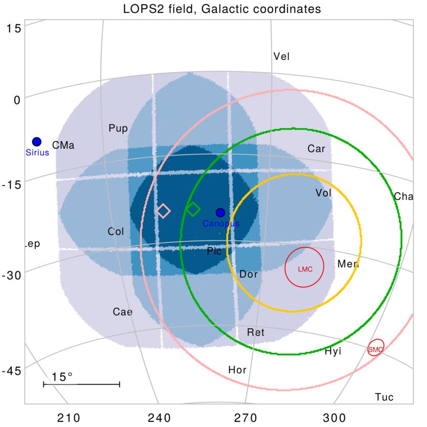
Figure 1: LOPS2  (sourced from PLATO SWT)

A cone search was performed for all G<9 stars in Gaia DR3 within LOPS2, yielding 14681 total stars. Cuts were then placed in the resulting catalog to select those stars that fit the predetermined fgPIC requirements. A final cut was utilized to select those stars that will be seen by PLATO’s CCDs during its initial observations, yielding 1503 total stars. From this, a randomly drawn sample of 30 stars was chosen for testing.  For the stars in this sample, light curves were obtained from TESS full frame images using the Eleanor python library (Feinstein et al. 2019). For each star in our sample, contaminants within 1 arcminute were obtained from Gaia Data Release 3 and the Stellar Pollution Ratio (SPR) was calculated. For a star with  contaminants, SPR is defined as

where F_* is the flux of the target star and F_i is the flux of the i-th contaminant.

Variability Analysis

To quantify stellar variability, we utilized an estimator known as FliPer (Flicker in the Power Domain) (Bastien et al. 2018). FliPer is defined as the averaged power spectral density (PSD) from some arbitrary initial frequency to the Nyquist frequency, corrected for photon noise. Photon noise for our TESS photometry was calculated using an empirical relation found by Kunimoto et al 2022.

FliPer serves as a robust measure of stellar variability as it has shown a strong correlation with fundamental stellar properties, particularly surface gravity.

Figure 2: FliPer vs. log(g) for stars in TESS Sector 33

Simulation

Simulated PLATO imagettes were created using the PlatoSim python library. Each round of simulations was performed with all sources of instrumental noise turned off and a constant background to minimize systematic effects. Three rounds of simulations were performed on each star in the sample. In the first round, the stars were constant. In the second round, the TESS photometry was introduced. Finally in the third, constant contaminants were added. 200 exposures per star were simulated for the first round, and 40320 exposures were simulated for the next two, as this number was close to the upper limit before memory issues were encountered.

Pointing Stability

Centroid coordinates for each simulated exposure are obtained through a PSF fitting algorithm. In this algorithm, an observation h(i, j) of a given pixel is modelled as a Gaussian PSF

with centroid position (u_c, v_c), PSF width σ, intensity I, background D, and random noise ξ.  The centroid is then determined by minimizing the distance function

for each pixel y(i, j) and unknowns α = (u_c, v_c, σ, I, D). (Grießbach et al. 2021). Since the FGS relies on measuring the guide stars’ centroids for attitude determination, we choose the transverse T of the centroid coordinates x and y 

in the boresight reference frame as an estimator of pointing stability.

Results

For each simulated dataset, the Spearman correlation coefficient  between the centroid noise and the base-10 logarithm of the FliPer was calculated. For the constant light curves, no significant correlation  was found, as expected. Low correlation was found for the variable cases without contaminants and with contaminants. However, correlation increases significantly for the case with contaminants when only considering stars with SPR >0.002.

Figure 3: FliPer vs. noise for sample with constant light curves.

Figure 4: FliPer vs. noise for sample without contaminants

Figure 5: FliPer vs. noise for sample including contaminants

Case	ρ
Constant light curves	0.0107
Variable targets with no contaminants	0.289
Variable targets with contaminants	0.240
Variable targets with bright contaminants	0.400