Jupiter’s south polar region (~60-80ºS): Wind patterns from JunoCam maps

Introduction

Previous studies of Jupiter’s wind patterns, from the Hubble Space Telescope and Cassini, revealed the southernmost two prograde jets at 58ºS and 64ºS (planetocentric), which we now designate as the S5 and S6 jets.  A few degrees further south they showed a retrograde flow, but the wind pattern further poleward was not well defined. It is important to characterise the flows in this region in order to understand the dynamics of the polar atmosphere and the processes that maintain the pentagon of cyclones around the south pole [1,2].  Here we use Juno (JunoCam) images to characterise the S5 and S6 jets and the wind patterns further south, up to the edge of the pentagon.

JunoCam takes hi-res images over the south polar region (SPR) at every perijove (PJ), which reveal the typical patterns of the region, in RGB and usually in the 0.89-µm CH₄ absorption band.  For each perijove we [G.E.] convert the RGB images into south polar projection maps, which can be ‘blinked’ or animated to visualise motions over ~0.5 to 2 hours.  They are also compiled into a composite map of most of the SPR. We use maps that go down to 60ºS at the edges (and further at the corners so part of the S5 jet is included).

 

Organisation of the SPR  [e.g. Fig.1]

Here we summarise general conclusions from JunoCam at all perijoves up to PJ23, from alignments of the RGB maps, the wind motions in animations, and the CH₄ maps.

The S5 jet is narrow and coincides exactly with a slightly sinuous boundary in methane images, the band to the south being methane-dark.  The S6 jet is faster, broader and highly undulating in latitude.  It generally coincides with the sinuous edge of the methane-bright South Polar Hood (SPH).   In CH₄ maps the wave pattern previously recorded [3] is always present around most or all of the circumference, with greater or lesser regularity.  Often the pattern is regular with wavelengths of 20-36º longitude (the mean from 8 perijoves is 25.5º ±2.6º) and amplitudes up to 3º latitude peak-to-trough. 

The SPR in RGB is dark, with an irregular edge that lies between the S5 and S6 jets.  It appears relatively bluer south of the S6 jet, apparently because SPH overlying it is a relatively bluish haze.

Poleward of the S6 jet, there is an irregular cyclonic belt of folded filamentary regions (FFRs) at ~65-70ºS.  They show typically rapid circulation and the retrograde part of this along their south edges could be regarded as a retrograde jet at ~71ºS; however this is only present within the FFRs, not between them.  Several AWOs are usually present close to the south edge of this belt of FFRs.

Further south, where the dominant features are scattered irregular FFRs and a few anticyclonic white ovals (AWOs), there are no permanent nor rapid nor extended jets.  There are sometimes short, weak prograde flows in mid-latitudes, ~74-77ºS, a few tens of degrees long. Some of these appear to be merely the flanks of flows within FFRs just to the south; others are oblique. There is no jet around the south polar pentagon.

 

Wind-speed measurements  [e.g. Fig.2]

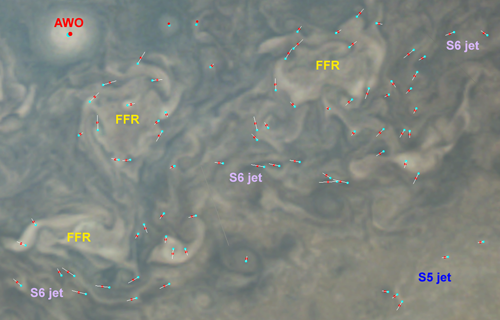
For each of PJ15, PJ16, and PJ17, a pair of single-image maps was aligned and blinked, and hundreds of points were marked on each map manually for feature tracking. Points were chosen on and near the most rapid currents, i.e. the peaks of the S5 and S6 jets and the outer parts of FFRs, so as to define these flows. 

We find that the S6 jet is rapid at all longitudes, and of variable width.  It traces large waves in latitude, generally coinciding with the wave pattern around the edge of the methane-bright SPH, though with a few local exceptions.  Mean peak wind speeds (measured along the jet rather than strictly eastward) range from 42 (±12) to 49 (±11) m/s. These are higher than previous speeds from Cassini and HST (25 to 42 m/s), probably because those were zonal averages diminished by the sinuosity of the jet.  This sinuosity of the S6 jet (and more weakly, the S5 jet) contrasts with the straight flow of all lower-latitude prograde jets.

Wind speeds were also measured in FFRs in the main belt and further south.  They were generally in the range of ~20-60 m/s, without obvious dependence on wind direction or latitude.  Mean speeds in each FFR ranged from 31 to 43 m/s, averaging 37 (±13) m/s.  (However, more diverse speeds may exist in some unmeasured FFRs.)  These speeds are comparable to those measured in other cyclonic structures at lower latitudes.

Conclusions

The S6 jet is highly sinuous, coinciding with the prominent waves around the edge of the methane-bright SPH.  There are no prograde jets closer to the pole. A belt of FFRs immediately south of the S6 jet includes fast retrograde speeds around ~71ºS.

The JunoCam maps alone cannot trace slower motions of larger features, notably FFRs, but this can be partially achieved with inclusion of ground-based maps: see our companion abstract in session ODAA3 [4].

 

References

 

Fig.1.  Polar projection map from PJ20.  Yellow circles mark the circumpolar cyclones. Inset:  CH₄ map at reduced scale. 

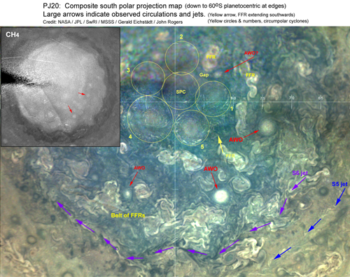
Fig.2.  Excerpt from a map at PJ16 with points measured for feature tracking indicated.