NEO Colors from The Mission Accessible Near-Earth Object Survey (MANOS)

The Mission Accessible Near-Earth Object Survey (MANOS) conducts characterization observations of objects on low delta-v orbits and in the sub-km size regime where knowledge of physical properties is sparse. Spectroscopic characterization of these objects serves to constrain the distribution of taxonomic and compositional types across the population of the most frequent Earth-impacting asteroids, including the direct precursors of meteorites. Such data can probe how spectral properties may be dependent on factors such as object size (Devogele et al. 2019), Earth encounter distance (Binzel et al. 2010), and/or perihelion distance as a proxy for peak surface temperature (Graves et al. 2019). Constraints on the ensemble spectral properties of potential Earth impactors, as well as improved understanding of how those properties evolve over time, has implications for assessing the planetary defense risk associated with the NEO population.

We will present the results of MANOS spectrophotometric observations for a sample of 199 NEOs (Figures 1 and 2). Observations were performed between 2014 and 2025 from the 4.3-m Lowell Discovery Telescope (LDT), the 4.1-m Southern Astrophysical Research Telescope (SOAR), and the 4-m Mayall Telescope. At all facilities we collected images using the SDSS griz filter set with respective band centers at 0.48, 0.62, 0.76 and 0.91 microns. These multi-band data were used to derive colors and to assign a spectral taxonomic type to each object based on a down-sampling of taxonomic templates from the Bus-DeMeo system (DeMeo et al. 2009). Observing strategies were employed to constrain the lightcurves of targets, which proved necessary to properly account for rotational brightness variations during the collection of non-simultaneous images in each filter. For example, we either measured a full rotational lightcurve before collecting a color sequence, or we interleaved images in a single reference filter to track and correct for lightcurve variations (e.g. a filter sequence of seven exposures in order r-g-r-i-r-z-r). Our sample of colors accessed objects as faint as r~22, which is about 1-2 magnitudes fainter than is typically observable with spectroscopic techniques. However, the reduction of spectral information down to just four channels can limit the ability to achieve unique spectral taxonomic classifications and is not well suited to detailed compositional analysis.

This work highlights several key findings. First, the distribution of taxonomic types from the color data is consistent with previously published MANOS spectroscopic results (Devogele et al. 2019). However, this distribution is distinct from analogous surveys that sample the larger end of the NEO size distribution (H<22). In particular we find a deficit of S-type asteroids and an overabundance of X-complex asteroids amongst sub-km NEOs. It remains unclear the extent to which this is a size-dependent compositional trend in the NEO population, a size-dependence on physical surface properties such as regolith grain size, and/or a consequence of various observational biases that can be more pronounced for small (H>20) objects.

Our second major finding is related to the influence of lightcurve variations on derived colors. Our approach of non-simultaneous multi-filter imaging found that ~75% of the sample required treatment of lightcurve variability to derive reliable colors. Not accounting for this variability would produce significantly different results, where some objects would appear as part of an entirely different taxonomic complex. This would clearly have consequences for interpretation of individual objects, but also manifests as a systematic bias in the distribution of spectral types based on colors derived from non-lightcurve corrected data. Specifically, we see an over-abundance of C-complex spectral types when lightcurve variability is not treated: with lightcurve correction we find 10±5% (1-sigma) of the sample is classified as C-type, without lightcurve correction this fraction increases to 27±7%. Finding a reason for this over-abundance is an area of ongoing work. However, it is clear that lightcurve variability must be considered in any color survey that involves non-simultaneous observations across multiple filters. Of course this issue is eliminated for instruments that can obtain simultaneous multi-band images.

Finally, we identified a number of unusual objects in our sample. This includes objects observed on multiple epochs that demonstrated significantly different colors across epochs. For example, the colors 2011 CG2 were best fit by a Cgh-type on one epoch and a Q-type on a second epoch. Such variability is highly unexpected and is not well understood. We also note the unusual colors of 2022 BX5, which appears as the isolated object in the upper right of Figure 2. These are the reddest colors measured for any NEO to date and are most consistent with D-type spectra that are more common in the outer Solar System.

This work acknowledges funding support from NASA grants 80NSSC21K1328, NNX17AH06G, and NNX14AN82G.

References:

Binzel et al. (2010), Nature 463, 331.

Binzel et al. (2019) Icarus 324, 41.

Birlan et al. (2024) A&A 689, A334.

DeMeo et al. (2009) Icarus 202, 160.

Devogele et al. (2019), AJ 158:196.

Graves et al. (2019), Icarus 322, 1.

Ivezic et al. (2019) AJ 122, 2749.

Navarro-Meza et al. (2024) AJ 167:163.

Perna et al. (2018) Planetary and Space Science 157, 82.

Sanchez et al. (2024) PSJ 5:131.

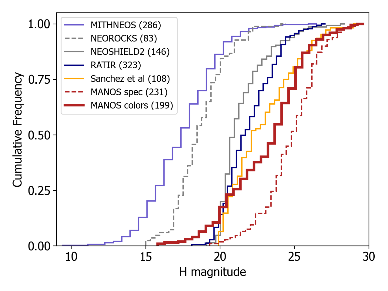
Figure 1: Cumulative size frequency distributions of key NEO spectral surveys. The number of objects sampled by each survey are given in parentheses in the legend. MANOS generally focuses on sub-km objects (H>20). The sample for our spectrophotometric survey is shown as the bold red curve. References for each survey: MITHNEOS (Binzel et al. 2019), NEOROCKS (Birlan et al. 2024), NEOSHIELD2 (Perna et al. 2018), RATIR (Navarro-Meza et al. 2024), Sanchez et al. (2024), and MANOS spectra (Devogele et al. 2019).

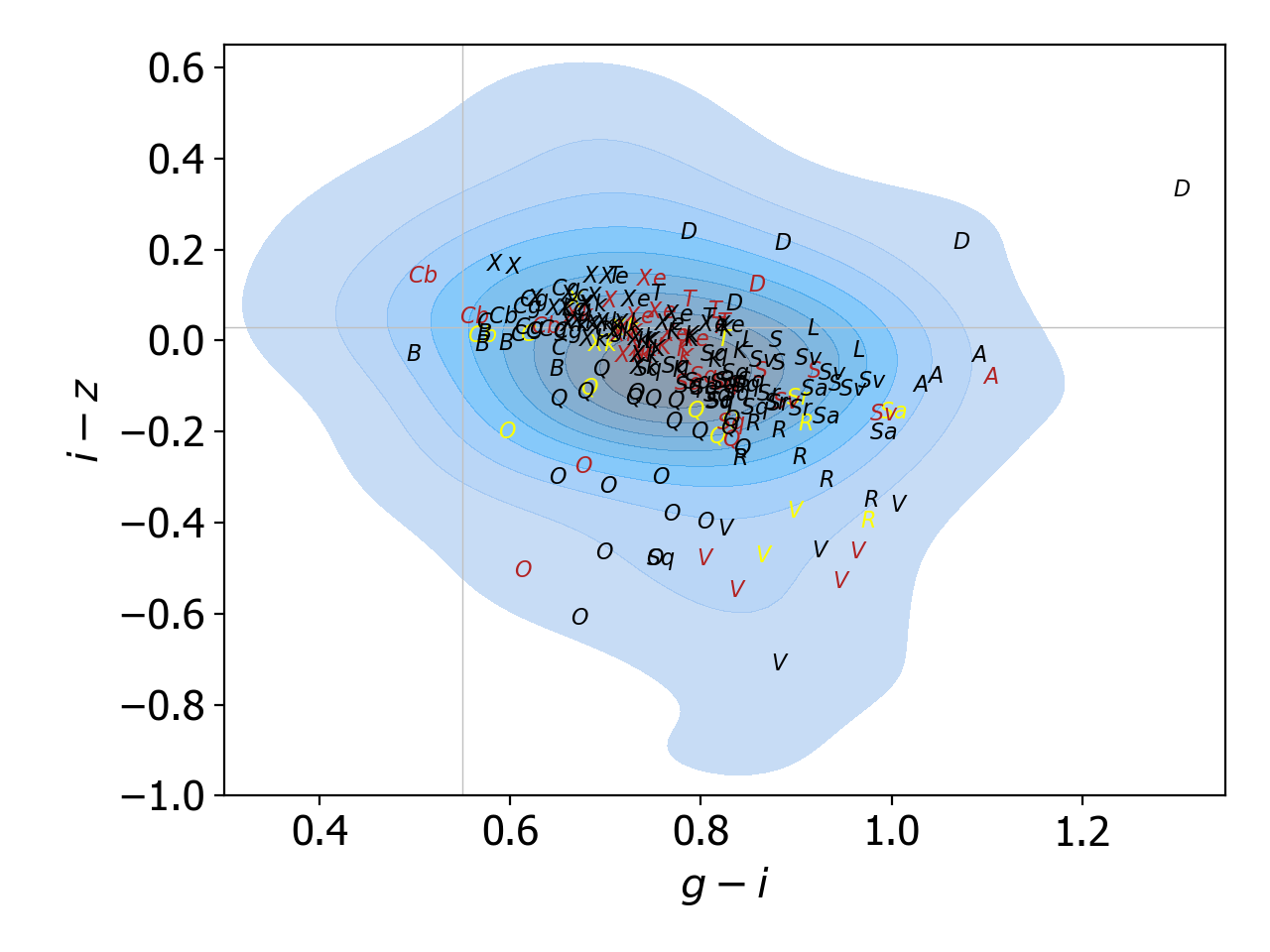
Figure 2: g-i versus i-z color-color plot for the 199 objects observed in the MANOS spectrophotometric survey. The taxonomic assignment for each object is indicated by the plotted letters. Data from LDT are in black, from SOAR in red, and from Mayall in yellow. The blue density contours in the background represent the colors of 223 NEOs from the Sloan Digital Sky Survey Moving Object Catalog (Ivezic et al. 2001).