Stability Maps for Terrestrial Planets in Star-Giant Planet configurations

Introduction

We present a new approach to test the orbital stability of a newly discovered planet in a two-body system. This work is based on stability map calculations that were used for building up the so-called Exocatalogue [1] which has been compiled for a dynamical model consisting of a star with, a giant planet, and a small Earth-like planet.

Stability calculations have been performed for various values of (i) the mass ratio μ = m₁ / (m₀ + m₁) of the star (m₀) and the giant planet (m₁), (ii) the eccentricity e₁ of the giant planet, (iii) the semi-major axis a of the Earth-like planet, and (iv) the mean anomaly M₁ of the giant planet. Stability maps were calculated for 23 discrete mass-ratios (from 0.0001 to 0.05) using the chaos indicators RLI (Relative Lyapunov Indicator [2]) and FLI (Fast Lyapunov Indicator [3]) to distinguish between regular and chaotic motion. These stability maps were also used to check whether the habitable zone (HZ) of a star is fully, partly, or not in a stable area.

The advantage of the new approach is that smooth boundary lines separating stable and chaotic regions are determined via AI methods so that we are no more restricted to certain discrete mass-ratios, since the AI model can calculate the stability map for any μ between 0.0001 and 0.05.

 

Method

The existing stability maps do not show a clear smooth border line between regular and chaotic motion, moreover, the border region itself looks rather chaotic (see Fig. 1). However, a smooth border line in the (a, e₁)-plane can be determined by the following procedure:

First, for each value of μ the average of all existing stability maps (different M₁ values) is computed. Though, the boundary region gets smoothed, it still has a chaotic, fractal-like shape.

We then apply a machine learning (ML) method, namely a Support Vector Machine (SVM; see https://scikit-learn.org/stable/modules/svm.html) to extract the decision boundaries between the regular and chaotic regions of the stability maps for the various values of μ for inner and outer orbits (with respect to the giant planet’s orbit). SVMs are supervised ML models that are commonly employed for classification problems. When classifying, the SVM constructs a hyperplane that represents the boundary surface between the different classes. A basic element in the SVM is the so-called kernel function that is the crucial factor in the classification procedure. In our specific case there are two classes, regular and chaotic, in a two-dimensional plane, thus, a one-dimensional decision boundary will be determined by the SVM model for each stability map.

To get a SVM decision boundary that follows the computed fractal boundary region close enough we use a polynomial SVM kernel of degree three. Finally, we computed 46 decision boundary lines, for the 23 values of μ for inner and outer orbits. With these values stability map plots (see Fig. 2) have been created where (i) the boundary lines are drawn, (ii) the stable/chaotic regions are colored (orange: stable, purple: chaotic), and (iii) a set of selected mean motion resonances (MMRs) are superimposed.

To calculate the stability maps for an arbitrary planetary system s which has a specific mass ratio μ_s and a specific giant planet semi-major axis a_s, the closest neighboring μ values for which calculated stability boundaries lines exist will be determined, and the boundary line for the system’s mass ratio μ_s will be computed by interpolating the underlying two-dimensional arrays of the neighbor’s decision boundary data. The semi-major axis will be scaled correspondingly to the value a_s.

Results

The stability maps for a planetary system with mass ratio μ = 0.0005 with data of the original Exocatalogue including the boundary (white curve) separating regular and chaotic regions computed by AI is shown in Fig. 1. These maps serve as basis for the calculations of planetary systems of interest. An example of AI stability maps of a real existing system is shown in Fig. 2 for the planetary system HD 93083 where a giant planet is orbiting the host-star at 0.477 au, which has a mass ratio μ = 0.000504, and which uses the data of Fig. 1 for determining its stability boundary

         

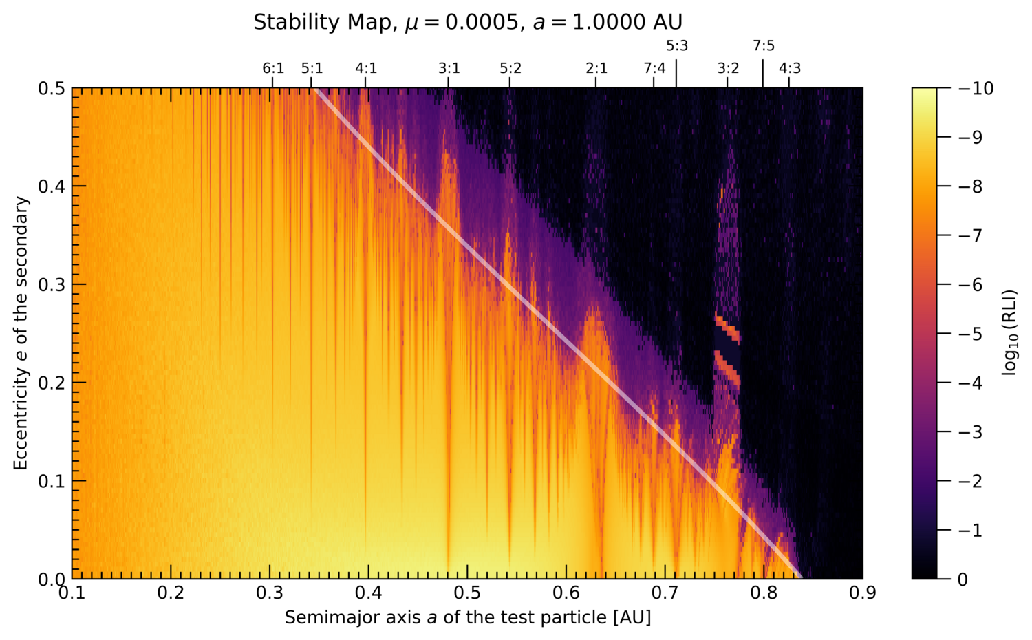
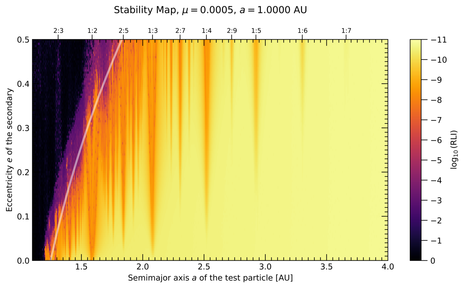
Figure 1: Stability maps (left: inner, right: outer region) for μ = 0.0005, the giant planet at 1 au according to the Exocatalogue. Yellow/orange indicates regular motion and purple/black chaotic regions. The white lines are the stability boundaries computed by the AI model.

                

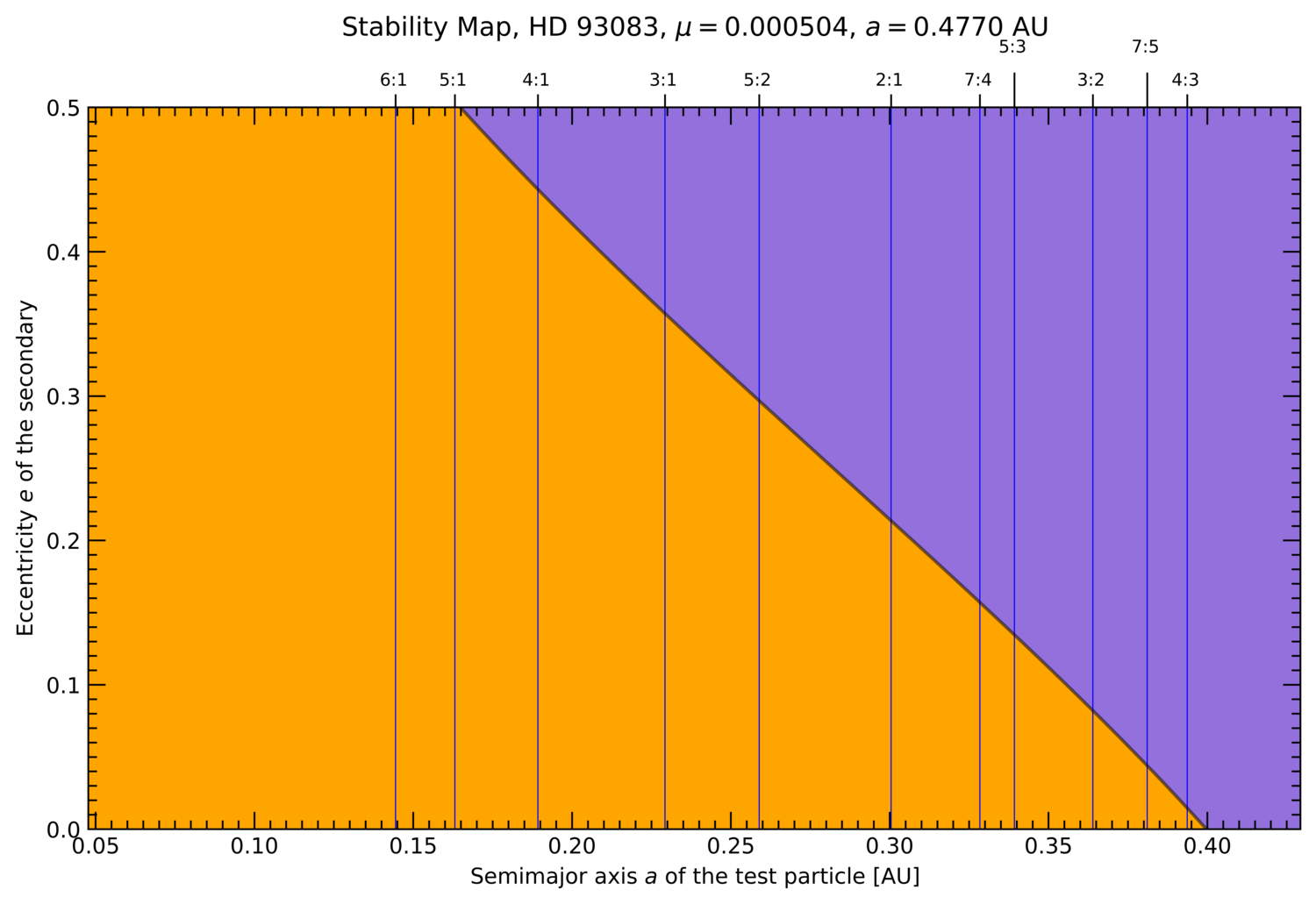
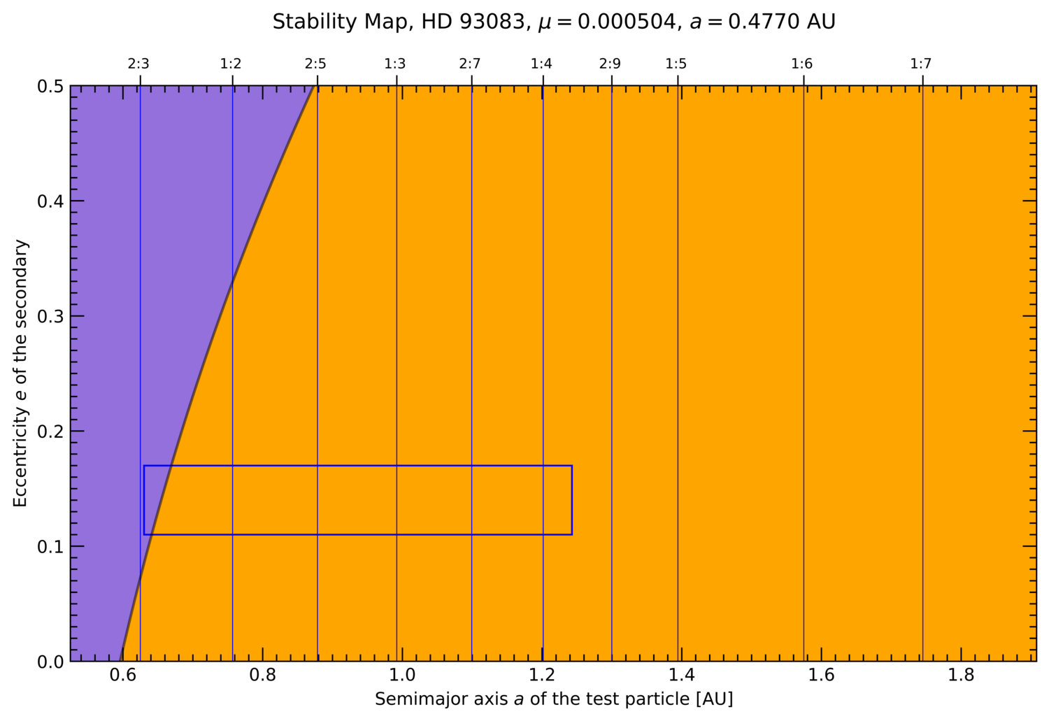
Figure 2: Stability maps (left: inner, right: outer region) generated by AI for HD 93083 (μ = 0.000504) with a giant planet at 0.477 au. The boundaries between regular (orange) and chaotic (purple) motion have been generated by the AI model. The rectangle located in the outer region marks the HZ.

Conclusion

Employing AI methods we are able to determine stability maps for any continuous value of the stellar to giant-planet mass ratio μ between 0.0001 and 0.05.

We plan to build a publicly available Web service, where users can enter the basic data for a planetary system s of interest, i.e. μ_s, a_s, and optionally the boundaries of the HZ, and the service computes in real-time the stability maps of that specific system, and creates plots for the inner and outer region containing the stability boundary lines, the colored areas of regular and chaotic orbits, a set of vertical lines representing MMRs, and optionally the edges of the HZ.

Acknowledgements

This research was funded by the Austrian Science Fund (FWF) [PAT3059124].

 

References

[1] Sándor, Zs., Süli, Á., Érdi, B.; Pilat-Lohinger, E., Dvorak, R.: 2007, MNRAS, 375, 1495.

[2] Sándor, Zs., Érdi, B., & Efthymiopoulos, C.: 2000, CeMDA, 78, 113

[3] Froeschlé, C., Lega, E., Gonczi, R.: 1997, CMDA, 67, 41.