Constraining Enceladus' heat flow between its tiger stripes

In 2005 data returned by the Cassini spacecraft showed that Enceladus’ southern polar region is highly active. The activity is concentrated along four fractures located close to Enceladus’ south pole commonly known as tiger stripes, which are also the source of Enceladus’ plumes. Accurately constraining the endogenic heat flow from this active region (often call South Polar Terrain, SPT) has proved challenging, and estimates of the SPT total heat flow vary from 5.8 ± 1.9 GW to 15.8 ± 3.1 GW (Spencer et al., 2006; Howett et al., 2011). One reason for these discrepancies is likely that the SPT has been in sunlight, and thus its emission is a combination of passive (reradiated sunlight) and endogenic components. Isolating the endogenic component is non-trivial and relies on either modeling (and removing) the passive component (as per the 15.8 GW estimate), or only counting as endogenic any emission at temperatures greater than likely maximum passive emission temperatures (as per the 5.8 GW, so this doesn’t include any low temperature, <80 K, endogenic emission).

Intriguingly another estimate of the heat flow from (only) Enceladus’ tiger stripes estimate their heat flow to be 4.2 GW (Spencer et al., 2018). This means that if the total heat flow is close to 15.8 GW (Howett et al., 2011) then a lot of the heat flow must be coming from somewhere else. The most logical place for this extra emission is the region between the stripes, called interstitial (or funiscular) terrain. Models of how this region formed require high heat flows: 200 and 500 mW m^-2 (e.g. Barr and Preuss, 2008; Bland et al., 2015; Le Gall et al., 2017). To translate these heat flows to total power we assume the emission is uniform across the entire interstitial region, and the interstitial region is the area between Damascus and Alexandria but excludes the sulci themselves (which are assumed by 590 km long and 2 km wide) to total 16,067 km². With these assumptions the predicted heat flows are  equivalent to 3.2 and 8.0 GW of emission. This is an enormous amount of heat, which has never been quantified, and has huge implications for Enceladus’ total heat emission rate, and hence long-term thermal and orbital evolution. Quantifying this heat flow is the goal of our work.

Since 2009 Enceladus’ SPT has been in winter, which is important in this study for two reasons: 1) it reduces the magnitude of the passive emission and 2) it reduces the difference in passive emission predicted by thermophysical models using a variety of feasible surface parameters. This results in the uncertainty of the passive emission prediction dramatically reducing, from in winter (2015) assuming albedos between 0.70 and 0.80, and thermal inertias between 1 and 100 J m⁻² K⁻¹ s^−1/2 (MKS). During winter and late-fall Cassini’s Composite Infrared Spectrometer (CIRS) took 5 observations of the SPT at a spatial resolution high-enough (<40 km) to put its fields of view between the stripes. These data, we propose to analyze, provide a “game-changing” opportunity to measure Enceladus’ heat flow, as the passive emission in them is minimized.

We present the results of our preliminary study to compare the surface temperatures derived from one swath from one of these CIRS observations (taken in 2015, chosen because it covered all four tiger stripes) to that predicted by a small number of passive models. The results, given in Figure 1, show the observed temperatures are much greater than ones the models predict. Depending on the model, interstitial heat flows between 279±48 to 380±36 mW m^-2 are required to explain the difference (4.5±0.7 to 6.1±0.6 GW, assuming the same interstitial area described above). While these are high heat flows they are well within those predicted by terrain formation models, but cannot fully explain the discrepancy between the different endogenic emissions determined. These results clearly show Enceladus’ interstitial region have endogenic emission, and require more detailed future analysis.

References

Barr, A.C. and L.J. Preuss, On the origin of south polar folds on Enceladus. Icarus 208, 499–503, 2010.

Bland, M.T. et al., Constraining the heat flux between Enceladus’ tiger stripes: Numerical modeling of funiscular plains formation, Icarus 260, 232-245, 2015.

Howett, C.J.A. et al. High heat flow from Enceladus’ south polar region measured using 10–600 cm−1 Cassini/CIRS data, Journal of Geophysical Research 116, E03003, 2011a.

Le Gall, A. et al. Thermally anomalous features in the subsurface of Enceladus’s south polar terrain, Nature Astronomy 1, 0063, 2017.

Spencer, J.R. et al. Cassini Encounters Enceladus: Background and the Discovery of a South Polar Hot Spot, Science 311, 1401-1405, 2006.

Spencer, J.R. et al. Plume Origins and Plumbing (Ocean to Surface), in Enceladus and the Icy Moons of Saturn, Editors Schenk, Clark, Howett, Verbiscer and Waite, University of Arizona Press, 2018,

 

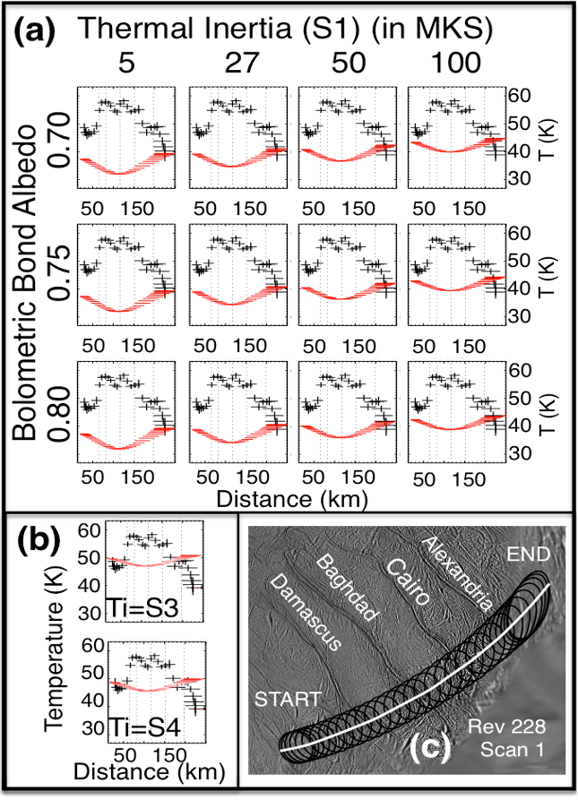
Figure 1: A comparison of passive modeled and CIRS derived surface temperatures, showing none of the models fit the interstitial temperatures. (a) Temperature derived from Rev 228 (Dec 2015) CIRS data (black) and those predicted by passive thermal models (red) for a range of albedo (rows) and thermal inertia (columns). In all models the thermal inertia is constant with depth (S1). “Distance” is calculated as the distance from the start of the white line in (c) to where the line intersects the nearest and furthest points of the field of view. Dotted lines indicate where the line crosses the tiger stripes, from left to right: Damascus (both branches), Baghdad, Cairo and Alexandria. (b) Same as the top plot, but for seasonal models with an albedo 0.80 and a thermal inertia profile that changes with depth (see Fig. 8 for details of S3 and S4). (c) Footprints of the CIRS FP1 field of view (black). Tiger stripe names are indicated.