
Stratospheric HCN and Evolution of a Mixing Barrier in Titan’s Equatorial Region from Low-Resolution Cassini/CIRS Spectra
 1,1,2,3,4
- 1School of Earth Sciences, University of Bristol, United Kingdom of Great Britain – England, Scotland, Wales (lucy.wright@bristol.ac.uk)
- 2Atmospheric, Oceanic, and Planetary Physics, University of Oxford, UK
- 3Planetary Systems Laboratory, NASA Goddard Space Flight Centre, Greenbelt, USA
- 4School of Geographical Sciences, University of Bristol, UK
1. Introduction
Titan is the only moon in our solar system with a substantial atmosphere. It comprises 98% Nitrogen (Niemann et al., 2005), and is rich in hydrocarbon (CxHy) and nitrile (CxHyNz) species. Such species photochemically react to produce organic aerosols which compose a thick orange haze suspended in Titan’s middle atmosphere.
Global Circulation Models (GCMs) predict the meridional circulation in Titan’s stratosphere and mesosphere is dominated by a single pole-to-pole circulation cell for most of the Titan year (Hourdin et al., 1995; Newman et al., 2011; Lebonnois et al., 2012), and observations are broadly consistent with this prediction (Teanby et al., 2012, Vinatier et al., 2015). These models suggest circulation across the stratospheric equator, but this is not entirely consistent with what is observed. Existing studies show a North-South asymmetry in stratospheric haze abundance (Lorenz et al., 1997; de Kok et al., 2010), suggesting a mixing barrier near the equator. Here, we present a radiance ratio method for approximating latitudinal distributions of stratospheric HCN. We apply this to the region +/-30 degN and use HCN as a tracer to investigate the evolution and behaviour of the equatorial mixing barrier over the Cassini mission.
2. Observations
The Cassini spacecraft explored Saturn and its moons from 2004 to 2017. Throughout its 13-year exploration, Cassini performed 127 close flybys of Titan, observing at infrared, visible and ultra-violet wavelengths. One of Cassini’s twelve instruments, the Composite Infrared Spectrometer (CIRS) (Flasar et al., 2004; Jennings et al., 2017; Nixon et al., 2019) collected almost 10 million Titan spectra in the mid and far-infrared ranges (10 – 1500 cm-1), at a varied spectral resolution between 0.5 – 15.5 cm-1. In this study, we analyse low spectral resolution (~15 cm-1) observations collected by two CIRS focal planes, sensitive to wavenumber ranges 600 – 1100 cm-1 (FP3) and 1100 – 1500 cm-1 (FP4). Generally, low spectral resolution observations require shorter scan times so can be performed at a closer approach distance to Titan, hence achieving higher spatial resolution. This allows small spatial variations in atmospheric constituents to be resolved. Low-resolution observations also have good coverage of Titan’s equatorial region throughout the entire Cassini mission (Figure 1).
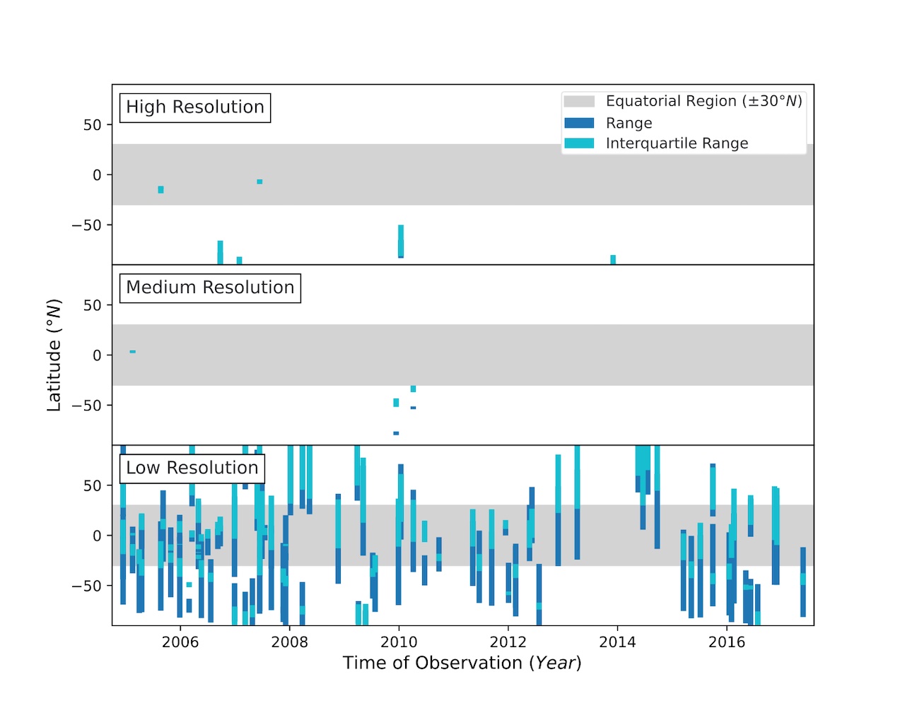
Figure 1: Mission coverage for the Cassini CIRS low spectral resolution nadir mapping observations.
3. Optimising Line-by-Line Retrieval Efficiency
Line-by-line (LBL) inversions in spectral analysis are computationally expensive. The correlated-k approximation (Lacis and Oinas, 1991) is often used to decrease the computation time of retrievals, but we found that it is not sufficiently accurate for these low spectral resolution and high signal-to-noise ratio observations (Figure 2c, d). In LBL modelling, a key parameter is the underlying spectral grid spacing. Finer grid spacing improves the forward model accuracy, but at a greater computation cost. To improve the efficiency of LBL runs, we determine a maximum grid spacing (Figure 2a, b) for which a LBL inversion will produce a sufficiently accurate spectrum in the shortest computation time. Typically, a single forward model run takes 2 hours for LBL, compared to 2 seconds for k-tables.
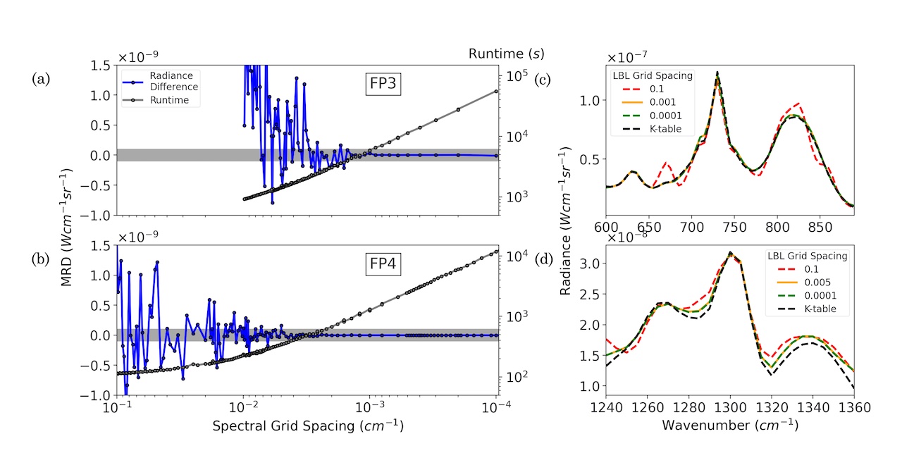
Figure 2: Comparison of spectra produced using a correlated-k (k-table) method and a line-by-line (LBL) method at varied spectral grid spacing. Maximum radiance difference (MRD) (a, b, blue line) between spectra produced at varied (0.1 – 0.0001 cm-1) and fine (0.0001 cm-1) grid spacing is assessed against a level of sufficient accuracy (a, b, grey area). The grid spacing determined to be optimal (0.001 cm-1 for FP3, 0.005 cm-1 for FP4) produces an almost identical spectrum to very fine (0.0001 cm-1) grid spacing (c, d) but at a significantly reduced runtime (a, b). A spectrum produced using a coarse grid spacing (0.1 cm-1) is shown for comparison. The spectrum retrieved using k-tables is not sufficiently accurate for these low-resolution observations (c, d).
4. Estimating Stratospheric HCN with a Radiance Ratio
We construct a radiance ratio formula for approximating HCN abundance from CIRS spectra, such that a greater number of observations can be analysed rapidly. Radiance ratios can be a useful tool for approximating gas contributions to a spectrum. They do not have the reliability of full spectral retrievals but require significantly less computation time. We compare the radiance ratio latitude dependence to full LBL retrievals of HCN, for a subset of our observations, to assess the reliability of our ratio method. LBL retrievals are performed using the Nemesis radiative transfer and retrieval code (Irwin et al., 2008) with our pre-determined optimal grid spacing. We calculate the radiance ratio for a set of approximately 20 low spectral resolution mapping observations (3 are shown in Figure 3).
There appears to be a sharp change in HCN abundance near the equator (Figure 3). This hints at a potential mixing barrier in Titan’s stratosphere. Furthermore, the position of this potential barrier appears to migrate over time. We use the results of this study to investigate dynamic processes in the equatorial region of Titan’s stratosphere and its evolution over the entire Cassini mission.
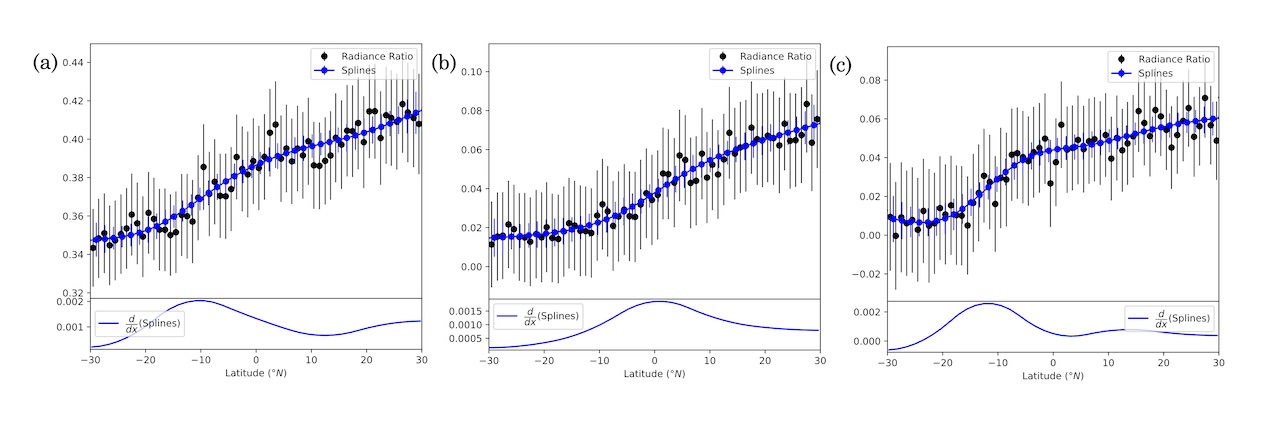
Figure 3: Our radiance ratio calculated for observations acquired on 08/2005 (a), 05/2006 (b) and 07/2012 (c). The radiance ratio is smoothed by fitting splines (Teanby, 2007). The gradient of each smoothed fit is also shown (bottom).
Acknowledgements
This research was funded by the UK Sciences and Technology Facilities Council.
References
de Kok, R., et al. (2010). https://doi.org/10.1016/j.icarus.2009.10.021
Flasar, F. M., et al. (2004). https://doi.org/10.1007/s11214-004-1454-9
Hourdin, F., et al. (1995). https://doi.org/10.1006/icar.1995.1162
Irwin, P., et al. (2008). https://doi.org/10.1016/j.jqsrt.2007.11.006
Jennings, D. E., et al. (2017). https://doi.org/10.1364/AO.56.005274
Lacis, A. A., & Oinas, V. (1991). https://doi.org/10.1029/90JD01945
Lebonnois, S., et al. (2012). https://doi.org/10.1016/j.icarus.2011.11.032
Lorenz, R. D., et al. (1997). https://doi.org/10.1006/icar.1997.5687
Newman, C. E., et al. (2011). https://doi.org/10.1016/j.icarus.2011.03.025
Nixon, C. A., et al. (2019). https://doi.org/10.3847/1538-4365/ab3799
Niemann, H. B., et al. (2005). https://doi.org/10.1038/nature04122
Teanby, N. A. (2007). https://doi.org/10.1007/s11004-007-9104-x
Teanby, N. A., et al. (2012). https://doi.org/10.1038/nature1161
Vinatier, S., et al. (2015). https://doi.org/10.1016/j.icarus.2014.11.019
How to cite: Wright, L., Teanby, N. A., Irwin, P. G. J., Nixon, C. A., and Mitchell, D. M.: Stratospheric HCN and Evolution of a Mixing Barrier in Titan’s Equatorial Region from Low-Resolution Cassini/CIRS Spectra, Europlanet Science Congress 2022, Granada, Spain, 18–23 Sep 2022, EPSC2022-463, https://doi.org/10.5194/epsc2022-463, 2022.