OPS2

The Cassini/UVIS observations of Titan’s atmosphere extend from 2005 to 2017 providing a broad spatial and temporal view of the upper atmosphere including the seasonal change from Southern summer at the Cassini-Huygens arrival in 2005, to equinox (August 2009), to Northern summer (summer solstice in May 2017). The general emission characteristics of the illuminated Titan side are common among the observations: Near the ionospheric peak (~1100 km) the atomic and molecular emissions dominate the observed signal (Fig. 1). Atomic emissions include Ly-α (1216.7 Å) scattering from atomic hydrogen and emissions from N and N⁺ excited during the photolysis of N₂, with major contributions at 1085 Å (N⁺, ³D⁰ à ³P), 1200 Å (N, ⁴D⁰ à ⁴S⁰ ) and 1493 Å (N, ²P à ⁴S⁰). Molecular emissions are dominated by the Lyman-Birge-Hopfield (LBH, α ¹Π_g à X ¹Σ_g⁺) and Vegard-Kaplan (VK, A³Σ_u⁺ à Χ ¹Σ_g⁺) bands, both in the FUV. These observations provide valuable constraints for the atmospheric structure.

We use a detailed forward model to simulate the observed emission, which relies on constraints from models of solar energy deposition (Lavvas et al. 2011) and N₂ aiglow (Lavvas et al. 2015). Our simulations demonstrate that all observed emissions result from the excitation of atomic and molecular nitrogen and from scattering by atomic hydrogen (Fig. 1). Using such a detailed forward model for the inversion of the atmospheric properties is, however, inefficient due to the large computational times involved. Instead we propose a simplified retrieval focusing on specific atomic lines in the FUV range, which allows for an efficient atmospheric characterization with minimal computational effort, while preserving the benefits of the detailed forward modeling.

Figure 1: Observed (black) and simulated (red) limb spectra on Titan’s dayside during the 2016, DOY-015 PRIME observations. The top panel presents the average spectrum at 1100 km (100 km wide bin) demonstrating the strong Ly-α emission and the emissions from atomic (dashed lines) and molecular transitions (thin blue lines for LBH and thin red lines for VK bands).

References

• Lavvas P., Yelle R.V., Heays A.N., Campbell L., Brunger M.J., Galand M., Vuitton V., 2015. N2 state population in Titan’s atmosphere. Icarus, 260, p.29-59.
• Lavvas P., Galand M., Yelle R.V., Hayes A.N., Lewis B.R., Lewis G.,R. Coates A.J., 2011. Energy deposotion and primary chemical products in Titan’s atmosphere. Icarus, 213, 233-251. 

How to cite: Lavvas, P. and Koskinen, T.: Titan’s atmospheric structure from Cassini/UVIS airglow observations, Europlanet Science Congress 2022, Granada, Spain, 18–23 Sep 2022, EPSC2022-447, https://doi.org/10.5194/epsc2022-447, 2022.

Introduction

    With 13 years of observations, the Ion and Neutral Mass Spectrometer (INMS) onboard the Cassini spacecraft has observed the upper atmosphere of Titan through two seasons: winter and spring. The complex atmosphere is mainly composed of N₂, CH₄, H₂ and Ar, but a lot more carbon and nitrogen bearing trace species have been observed by INMS and other instruments. Using data from the closed source neutral mode of INMS instrument, we studied the abundance and variation of traces neutral species in Titan ionosphere, between 1500 and 950 km of altitude. We will present an ongoing effort on the reanalysis of the entire INMS Titan's observation dataset. 

Method

To do so we recalibrated INMS data by taking into account the dead time correction, the ram pressure enhancement, the saturation correction, the increase of pressure in the chamber with the decreases of altitude, the sensitivity and the contamination by thruster firing (Cui et al., 2009,2012). In addition, species entering the instrument were ionized and fragmented into ions inside INMS chamber, making difficult the identification of different species in such complex mass spectra. To retrieve the molecular mixing ratios we used a Monte-Carlo sampling on the fragmentation pattern to deconvolve the signal.  To obtain a complete mass spectrum (m/z 1 to 99), we stacked INMS data, which increases the incertitude on the altitude. We used the mass spectra deconvolution code developed by Gautier et al., (2020), also employed by Serigano et al., (2020) when they treated Saturn INMS data.

This enabled the retrieval of vertical and seasonal variation of Titan's atmosphere minor components. We expect to be able to link our results with the seasonal variations observed by other instruments [such as CIRS (Mathé et al., 2020)] in lower atmospheric layers. 

References

Cui et al.(2009) Analysis of Titan’s neutral upper atmosphere from Cassini Ion Neutral Mass Spectrometer measurements. Icarus 200 (2009) 581–615

Cui et al.(2012) The CH₄ structure in Titan’s upper atmosphere revisited. J. Geophys. Res., 117, E11006, doi:10.1029/2012JE004222.

Gautier et al. (2020) Decomposition of electron ionization mass spectra for space application using a Monte-Carlo approach. Rapid. Com. Mass Spec. 34(8), e8659

Mathé et al., (2020) Seasonal changes in the middle atmosphere of Titan from Cassini/CIRS observations: Temperature and trace species abundance profiles from 2004 to 2017. Icarus, 344, 113547.

Serigano et al. (2020) Compositional measurements of saturn's upper atmosphere and rings from cassini INMS. Journal of Geophysical Research: Planets, 125(8), e2020JE006427.

How to cite: Coutelier, M., Gautier, T., Das, K., Serigano, J., and Horst, S.: Seasonal variation of trace species in Titan’s ionosphere, Europlanet Science Congress 2022, Granada, Spain, 18–23 Sep 2022, EPSC2022-479, https://doi.org/10.5194/epsc2022-479, 2022.

Titan’s stratospheric polar vortex is a prominent phenomenon of Titan’s global wind field, consisting of a westerly jet achieving speeds of nearly 200 m s^-1 [1, 2].  The strong westerly winds have been hypothesized to serve as a mixing barrier to molecules transported to the high winter latitudes by Titan’s stratospheric meridional overturning circulation [2].  Similar to Earth’s stratospheric polar vortex, the vortex on Titan is primarily driven by diabatic cooling at high winter latitudes, resulting in a steep meridional temperature gradient and, via the thermal wind relation, a strong vertical wind shear [3].  While the existence and evolution of the vortex has been constrained for one half of a Titan year by observations from the Cassini spacecraft, a rigorous analysis of the potential mechanisms that give rise to the strong stratospheric jet has not yet been performed.

Here, using simulations from the Titan Atmospheric Model [4], which has recently been updated to better simulate Titan’s stratosphere [5], we study the temporal evolution of processes proposed to be responsible for the evolution of Titan’s stratospheric polar vortex, including: solar shortwave heating (largely controlled by the presence of stratospheric aerosols), adiabatic heating from the descending branch of the meridional overturning circulation, and molecular longwave cooling [3].

References

[1] Sharkey, J. et al, (2021) Icar 354, 114030

[2] Schultis, J., et al., (2022) PSJ 3, 73

[3] Teanby, N. A., et al, (2017), Nat Comm 8, 1586

[4] Lora, J. M., et al., (2015), Icar 250, 516 – 528

[5] Lombardo, N. A., et al., (in review), Icar

How to cite: Lombardo, N. A. and Lora, J. M.: The Energy and Momentum Balance of Titan’s Stratospheric Polar Vortex as Simulated in a General Circulation Model, Europlanet Science Congress 2022, Granada, Spain, 18–23 Sep 2022, EPSC2022-655, https://doi.org/10.5194/epsc2022-655, 2022.

The objective of this study is to identify the dominant atmospheric wave modes driving and maintaining superrotation on Titan, by using a combination of space-time cross spectral wave analysis and spherical harmonic wave analysis techniques.

A defining feature of Titan’s atmospheric circulation is the presence of strong, planet-wide superrotation in the stratosphere. To achieve and sustain equatorial superrotation, angular momentum must be transported up the angular momentum gradient, which can only be accomplished by wave transport [2]. Newman et al. (2011)  showed that equatorial superrotation can be maintained via episodic “transfer events,” in which barotropic instability leads to the generation of planetary-scale waves that carry angular momentum and speed-up the equatorial flow [3]. Yet the origin and nature of these waves in the real atmosphere, and the exact mechanisms driving superrotation and upper atmospheric wave forcing, remain unknown.

We simulated the Titan atmosphere using the Titan Weather Research and Forecasting (TitanWRF) model and evaluated the temperature and momentum perturbations at different times during one full Titan year of simulation output. Fourier transforms of the temperature and wind fields showed that a strong correlation can be established between wave amplitude and angular momentum transfer events. Power spectral density for eddy heat and eddy momentum as a function of altitude, latitude, and phase speed or zonal wavenumber further emphasized the correlation. In our simulation, the largest angular momentum transfer event occurred around L_s~261°. Two additional transfer events were found at L_s~116° and L_s~192°, along with a number of smaller events occurring throughout the year.

References: [1] Charnay et al. (2015) Nature Geosci, 8, 362–366. [2] Gierasch (1975) J. Atmos. Sci., 32, 1038–44. [3] Newman et al. (2011) Icarus, 213, 636–654.

How to cite: Leung, C., Tamppari, L., Newman, C., and Lian, Y.: Angular Momentum Transfer in Titan’s Stratosphere, Europlanet Science Congress 2022, Granada, Spain, 18–23 Sep 2022, EPSC2022-716, https://doi.org/10.5194/epsc2022-716, 2022.

Molecular nitrogen (N₂) and methane (CH₄) are the two major gas of Titan’s atmosphere. Their dissociation in the upper atmosphere by photons and photo-electrons leads to a wealth of chemical reactions forming more complex molecules like nitriles and hydrocarbons, which subsequently combine to form Titan’s photochemical haze.

Isotopic ratios measured in N₂ and CH₄ are of particular interest to constrain the origin and evolution of Titan’s atmosphere. While the same isotopic ratios measured in photochemical species bring constraints on fractionation processes occurring through their formation and/or loss.      

We focus on the determination on the ¹⁴N/¹⁵N and the ¹²C/¹³C isotopic ratios in HCN and the ¹²C/¹³C ratio in HC₃N by analyzing their thermal emission acquired by the Cassini Composite Infrared Spectrometer (CIRS) from 2004 to 2017 (from the northern winter to the northern summer).  We used the entire CIRS dataset acquired with a limb-geometry viewing at the highest spectral resolution (0.5 cm^-1). This allows us to search for potential variations of these isotopic ratios with latitude or with season, which could help to identify potential fractionation processes. Our analysis incorporates the temperature and minor species volume mixing ratio profiles inferred previously by Mathé et al. (2020) from the same limb dataset. We will present our results regarding the isotopic ratios in HCN for all latitudes, while we will present the ¹²C/¹³C ratio in HC₃N only at high latitudes, as this nitrile is not detected at mid- and low-latitudes.

References:
- Mathé et al., 2020. Seasonal changes in the middle atmosphere of Titan from Cassini/CIRS observations: Temperature and trace species abundance profiles from 2004 to 2017. Icarus 344,  id. 113547.

How to cite: Vinatier, S., Mathé, C., Bézard, B., Jolly, A., and Gautier, T.: Isotopic ratios in Titan’s HCN and HC3N derived from Cassini/CIRS observations, Europlanet Science Congress 2022, Granada, Spain, 18–23 Sep 2022, EPSC2022-258, https://doi.org/10.5194/epsc2022-258, 2022.

Titan, the largest satellite of Saturn, has a dense atmosphere mainly composed of nitrogen and methane at a percent level. These two molecules generate a complex prebiotic chemistry, a global haze, most of the cloud cover and the rainfalls which model the landscape. Methane sources are located in liquid reservoirs at and below the surface and it sink is the photodissociation at high altitude. Titan’s present and past climates strongly depend on the connection between the surface sources and the atmosphere upper layers. Despite its importance, very little information is available on this topic. 

 In the last two decades, the observations made by the Cassini orbiter and the Huygens probe have greatly improved our knowledge of Titan’s system. The surface, haze, clouds, and chemical species can be studied and characterised with several instruments simultaneously. On the other hand, some compounds of its climatic cycle remain poorly known. This is clearly the case of the methane cycle, which is, however, a critical component of Titan’s climate and of its evolution. 

We reanalysed four solar occultations by Titan’s atmosphere observed with the infrared part of the Visual Infrared Mapping Spectrometer (VIMS) instrument. These observations were already analysed (Bellucci et al., 2009, Maltagliati et al., 2015), but here we used significantly improved methane spectroscopic data. We retrieved the haze properties (not treated previously) (Figure 1) and the mixing ratios of methane (Figure 2), deuterated methane, and CO in the stratosphere and in the low mesosphere.

Figure 1 : Haze extinction as a function of altitude, retrieved for the four observations, at wavelengths 0.884 μm (channel #97), 1.540 μm (channel #137) and 2.199 μm (channel #177). The extinction profiles retrieved by Seignovert et al. (2021) with Cassini/ISS, at wavelength 338 nm (CL-UV3 filters), are shown with green lines (labelled "S2020"). Those from Vinatier et al. (2010) or Vinatier et al. (2015), scaled at the wavelength 1μm, are shown with black lines ("V2010" or "V2015"). The profiles in cyan ("RP83"), are the extinctions retrieved by Rages & Pollack (1983) at 30◦N in August 1981 (wavelength 0.5 μm). The differences in the detached haze altitudes between VIMS-IR (Ls = 26°), Cassini/ISS (Ls = 14.8°) and Voyager 2/ISS (Ls = 18°) are their dates while the detached is falling down (West et al. (2018); Seignovert et al. (2021)). The grey line shows the haze profile by Doose et al. (2016) with DISR in 2005 at 10°S (labelled "D2016"). 

We find that the methane mixing ratio in the stratosphere is much lower (about 1.1%) than expected from Huygens measurements (about 1.4 to 1.5%). However, this is consistent with previous results obtained with CIRS. Features in the methane vertical profiles clearly demonstrate that there are interactions between the methane distribution and the atmosphere circulation. We find a layer rich in methane at 165 km and at 70°S (mixing ratio 1.45 ± 0.1%) and a dryer background stratosphere (1.1 − 1.2%). In absence of local production, this reveals an intrusion of methane transported into the stratosphere, probably by convective circulation. On the other hand, methane transport through the tropopause at global scale appears quite inhibited. Leaking through the tropopause is an important bottleneck of Titan’s methane cycle at all timescales. As such, it affects the long term evolution of Titan atmosphere and the exchange fluxes with the surface and subsurface reservoirs in a complex way.

Figure 2 : Methane mixing ratio retrieved with the four observation sets, with data between 0.88 and 2 μm (top) and between 2 and 2.8 μm (bottom). We also plot the methane mole fraction retrieved with the GCMS onboard Huygens (Niemann et al. (2010)) and with DIRS (Bézard (2014)) and CISR (Lellouch et al. (2014)). The green dashed profile, in the upper left graph, shows the evaluation made by Rannou et al. (2021). 

We also retrieved the haze extinction profiles and the haze spectral behaviour. We find that aerosols are aggregates with a fractal dimension of Df ≃2.3±0.1, rather than Df ≃2 as previously thought. Our analysis also reveals noticeable changes in their size distribution and their morphology with altitude and time. These changes are also clearly connected to the atmosphere circulation and concerns the whole stratosphere and the transition between the main and the detached haze layers. 

We conclude that, to fully understand these results, Global Climate Models accounting for haze and cloud physics, thermodynamical feedbacks and convection are needed. Especially, the humidificaton of the stratosphere, at the present time and its evolution under changing conditions at geological timescale appears as a key process, and our work provide strong constraints to guide studies.

References

Bellucci, A., Sicardy, B., Drossart, P., et al. 2009, Icarus, 201, 198 
Bézard, B. 2014, Icarus, 242, 64 
Doose, L. R., Karkoschka, E., Tomasko, M. G., & Anderson, C. M. 2016, Icarus, 270, 355 
Lellouch, E., Bézard, B., Flasar, F. M., et al. 2014, Icarus, 231, 323 
Maltagliati, L., Bézard, B., Vinatier, S., et al. 2015, Icarus, 248, 1 
Niemann, H. B., Atreya, S. K., Demick, J. E., et al. 2010, Journal of Geophysical Research (Planets), 115, E12006 
Rages, K. & Pollack, J. B. 1983, Icarus, 55, 50 
Rannou, P., Coutelier, M., Riviere, E., et al. 2021, Astrophysical Journal, 922
Rey, M., Nikitin, A., Bézard, B., et al. 2018, Icarus, 303, 114 
Seignovert, B., Rannou, P., West, R. A., & Vinatier, S. 2021, The Astrophysical Journal, 907, 36 
Vinatier, S., Bézard, B., de Kok, R., et al. 2010, Icarus, 210, 852 
Vinatier, S., Bézard, B., Lebonnois, S., et al. 2015, Icarus, 250, 95 
West, R. A., Balloch, J., Dumont, P., et al. 2018, Geophysical Research Letters, 38 

How to cite: Rannou, P., Coutelier, M., Lebonnois, S., Maltagliati, L., Rivière, E., Rey, M., and Vinatier, S.: Solar occultations observed by VIMS-IR: What haze and methane profiles reveal about Titan's atmospheric dynamics and climate., Europlanet Science Congress 2022, Granada, Spain, 18–23 Sep 2022, EPSC2022-130, https://doi.org/10.5194/epsc2022-130, 2022.

In July 2017, we used the Texes high-resolution spectrometer at the NASA Infrared Telescope Facility to observe Titan in the 19.3-µm (519 cm^-1) region where the ν₄ band of deuterated acetylene (C₂HD) is located. Six individual lines were clearly detected with a S/N ratio up to 10. Spectral intervals around 8.0 (745 cm^-1) and 13.4 µm (1247 cm^-1) were observed during the same run to constrain the disk-averaged temperature profile and acetylene (C₂H₂) abundance profile respectively. Telluric correction and flux calibration were obtained from observations of asteroid Hygiea. Constraints from Cassini/CIRS observations in 2017 around the sub-Earth latitude were also used to constrain the atmospheric model and check the flux calibration. The D/H ratio is derived from the C₂HD/C₂H₂ abundance ratio. Preliminary results of this analysis indicate a D/H ratio in acetylene around 1.7×10^-5 with an uncertainty of about 10%, in agreement with the previous, less precise, determination from Cassini/CIRS measurements. This ratio is slightly larger than that in methane (approximately 1.3×10^-5), which suggests some fractionation at work in the photochemical production of acetylene from methane.

How to cite: Bézard, B., Vinatier, S., Greathouse, T., Giles, R., Nixon, C., Lombardo, N., Jolly, A., and Despan, D.: The D/H ratio in Titan's acetylene from high spectral resolution IRTF/Texes observations, Europlanet Science Congress 2022, Granada, Spain, 18–23 Sep 2022, EPSC2022-363, https://doi.org/10.5194/epsc2022-363, 2022.

More than a decade after the arrival of the Cassini-Huygens mission in Saturn’s system, data returned by the Huygens probe during its descent remain a unique source of in-situ information on the lower atmosphere of Titan. Among the Huygens instrumental suite was the GCMS (Gas Chromatograph Mass Spectrometer) instrument which returned hundreds of mass spectra acquired in the atmosphere below 145 km of altitude.

We will present a reanalysis of GCMS data focusing on the methane vertical profile thanks to recent advances in our knowledge of Titan’s atmosphere and in mass spectrometry data treatment ^[1-3].

We retrieved methane mixing ratio slightly lower than the one reported by the original team^[4] and obtained its profile between 145 km and 30 km of altitude with a kilometric vertical resolution, and a sub-kilometric one between 30 km and the surface.

Such a vertical resolution unveiled clear oscillations in the methane mixing ratio in Titan’s troposphere and methane vertical concentration diverging from an ideal adiabat. Such features could for example be a sign of small-scale convective zones in the troposphere which could have triggered the gravity waves detected by Huygens in the stratosphere. We hope that the discovery of previously unnoticed features in GCMS data will also enable the reanalysis of data returned by other Huygens instruments such as HASI and DISR on Titan lower atmosphere.

^[1] Gautier et al. Decomposition of electron ionization mass spectra for space application using a Monte-Carlo approach. Rapid. Com. Mass Spec. 34(8), e8659 (2020)

^[2] Serigano et al. Compositional measurements of Saturn’s upper atmosphere and rings from Cassini INMS. JGR:Planets, 125 (8), E006427  (2020)

^[3] Serigano et al. Compositional Measurements of Saturn’s Upper Atmosphere and Rings from Cassini INMS: An extended Analysis of Measurements from Cassini’s Grand Finale Orbits. JGR:Planets, 127, E007238 (2022)

^[4] Niemann et al. Composition of Titan’s lower atmosphere and simple surface volatiles as measured by the Cassini-Huygens probe gas chromatograph mass spectrometer experiment. JGR 115, E12006, 2010

How to cite: Gautier, T., Serigano, J., Das, K., Coutelier, M., Hörst, S., Vinatier, S., Szopa, C., and Trainer, M.: Methane vertical profile in Titan’s atmosphere, Europlanet Science Congress 2022, Granada, Spain, 18–23 Sep 2022, EPSC2022-431, https://doi.org/10.5194/epsc2022-431, 2022.

Abstract

Titan's atmosphere has one of the most complex chemistry of the Solar System. On the one hand, its two main compounds, nitrogen and methane, are dissociated at high altitude by energetic solar photons and charged particles coming from the Saturnian magnetosphere. They produce a set of complex molecules that generates a layer of photochemical haze which completely covers Titan. On the other hand, there is a methane cycle similar to the hydrological cycle established on Earth (evaporation, condensation, precipitations and presence of rivers and lakes on the surface). Haze, methane and clouds are subject to coupled cycles that are not completely understood. They also contribute to the thermal equilibrium and long-term evolution of Titan. It is therefore important to better characterize these cycles and their interactions.

1. Principle of the work

The temperature profile of the satellite allows methane to condense, when it is transported upwards, on the aerosols which serve as a support for nucleation. Thus, after evaporation from the surface reservoirs, methane clouds are produce, precipitate, and return to the surface [Stofan et al., 2007]. The minor species created at high altitude also condense during their transport to the lower layers. These clouds have long been observed thanks to telescopes, and then to Cassini's instruments [Rodriguez et al., 2011]. Cloud activity has also been modeled from physical principles in the 2-D GCM (altitude-latitude) of IPSL [Rannou et al., 2006] and by simple models with other 3-D GCMs (e.g. [Mitchell et al., 2006] and [Lora et al., 2019]).

The Global Climate Model of Titan developed at the Institut-Pierre-Simon-Laplace is the ideal tool to understand how these cycles work and how clouds form on Titan. The transition of the model in 3 dimension has significantly improved our knowledge of the mechanisms of Titan's middle atmosphere [Lebonnois et al., 2012]. The microphysical processes associated with haze have been implemented long time ago. We now have added the clouds microphysics (methane, ethane, hydrocyanic acid, etc.) and we further plan to add convective aspects. Aside from that, the morphological structure (fractal dimension) of aerosols has also been questioned recently and is likely to modify the thermal equilibrium of the atmosphere, haze-dominated in the stratosphere. These are the two axes that we will explore in our work.

2. Results & Discussion

In this presentation, we will first discuss the impact of changing aerosol structure on the haze cycle and the consequences for the thermal equilibrium of the atmosphere. Recent works show that aerosols appear more compact than previously thought (with a fractal dimension D_f ∼ 2.3 instead of D_f ∼ 2.0). We studied the effects induced by such a change (change of vertical profiles, annual cycles, aerosol size, etc.). For example, Figure 1 shows the haze extinction in Titan's atmosphere depending on the pressure and latitude for two values of the aerosol fractal dimensions.

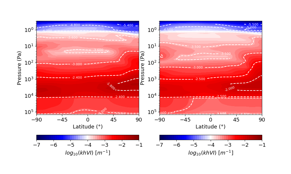
Fig. 1 Haze extinction at 4000 nm for D_f = 2.0 (left) and D_f = 2.3 (right) in the Titan Global Climate Model of IPSL.

We will detail the consequences on the structure of the haze and on the thermal equilibrium in the stratosphere (figure 2).

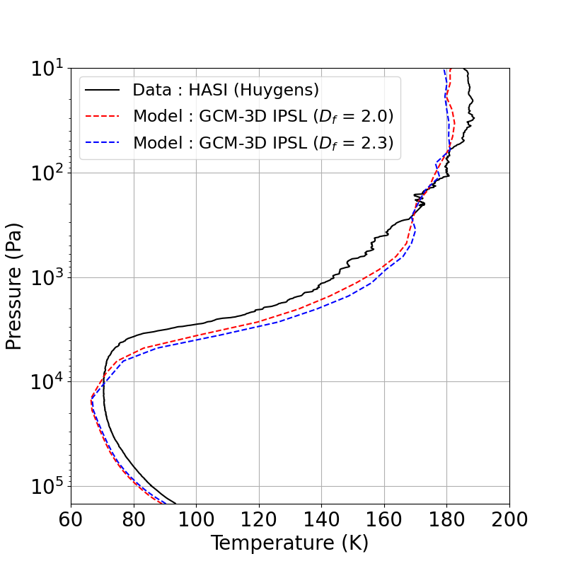
Fig. 2 Vertical temperature profile of Titan's atmosphere. The bold line corresponds to the profile measured by Huygens. The dotted lines correspond to the temperature profiles predicted with the IPSL model with D_f = 2.0 (in red) and D_f = 2.3 (in blue).

Next, we will describe the general principle of the cloud model used in the GCM and show the first results obtained. We will display the comparisons, on the one hand with observations and on the other hand with other models. This first step aims at recovering, in the 3-D GCM, the level of coupling previously reached in the 2-D model. We will also discuss the missing processes in the model and the strategy to account for. The main missing process is the convective cloud process, which have been observed.

This project is naturally in line with the upcoming observations of the JWST, the future Dragonfly mission and all other future missions. This model will allow the best possible characterisation of the climate expected in the Dragonfly landing region. Of course, it will also be a question of providing all possible elements necessary for the understanding of future observation of Titan.

References

E. R. Stofan, C. Elachi, J. I. Lunine, R. D. Lorenz, B. Stiles, K. L. Mitchell, S. Ostro, L. Soderblom, C. Wood, H. Zebker, S. Wall, M. Janssen, R. Kirk, R. Lopes, F. Paganelli, J. Radebaugh, L. Wye, Y. Anderson, M. Allison, R. Boehmer, P. Callahan, P. Encrenaz, E. Flamini, G. Francescetti, Y. Gim, G. Hamilton, S. Hensley, W. T. K. Johnson, K. Kelleher, D. Muhleman, P. Paillou, G. Picardi, F. Posa, L. Roth, R. Seu, S. Shaffer, S. Vetrella, and R. West, “The lakes of Titan,” Nature, vol. 445, no. 7123, pp. 61–64, Jan. 2007.

S. Rodriguez, S. Le Mouélic, P. Rannou, C. Sotin, R. H. Brown, J. W. Barnes, C. A. Griffith, J. Burgalat, K. H. Baines, B. J. Buratti, R. N. Clark, and P. D. Nicholson, “Titan’s cloud seasonal activity from winter to spring with Cassini/VIMS,” Icarus, vol. 216, no. 1, pp. 89–110, Nov. 2011.

P. Rannou, F. Montmessin, F. Hourdin, and S. Lebonnois, “The Latitudinal Distribution of Clouds on Titan,” Science, vol. 311, no. 5758, pp. 201–205, Jan. 2006.

J. L. Mitchell, R. T. Pierrehumbert, D. M. W. Frierson, and R. Caballero, “The dynamics behind Titan’s methane clouds,” Proceedings of the National Academy of Science, vol. 103, no. 49, pp. 18421–18426, Nov. 2006.

Juan M. Lora, Tetsuya Tokano, Jan Vatant d’Ollone, Sébastien Lebonnois, and Ralph D. Lorenz, “A model intercomparison of Titan’s climate and low-latitude environment,” , vol. 333, pp. 113–126, Nov. 2019.

Sébastien Lebonnois, Jérémie Burgalat, Pascal Rannou, and Benjamin Charnay, “Titan global climate model: A new 3-dimensional version of the IPSL Titan GCM,” , vol. 218, no. 1, pp. 707–722, Mar. 2012.

How to cite: de Batz de Trenquelléon, B., Rannou, P., Burgalat, J., and Lebonnois, S.: The IPSL's Titan Global Climate Model : Towards a 3-Dimensional microphysical cloud model, Europlanet Science Congress 2022, Granada, Spain, 18–23 Sep 2022, EPSC2022-445, https://doi.org/10.5194/epsc2022-445, 2022.

Titan, the largest satellite of Saturn, is known to host a rich and active meteorology, by all standards more dynamic than previously thought before the Cassini-Huygens mission. One key element of the dynamic Titan's atmosphere is the Planetary Boundary Layer (PBL), defined as the lowermost part of the atmosphere directly influenced by the presence of a surface below it. Turbulence in the PBL is a controlling factor for exchanges of momentum, heat, chemical species and aerosols between surface and atmosphere.

Following observations by the Cassini-Huygens mission, a debate has arisen on the vertical extent of the PBL mixing on Titan in daytime conditions. Radio-occultations by Voyager and Cassini, as well as insights from dune spacing, indicate that a mixed layer, following the dry adiabatic lapse rate, extends 2 to 4 km above the surface. Conversely, in situ mid-morning measurements on board the equatorial Huygens descent probe suggests a more complex structure, with a clear-cut mixed layer only found to extend 300 m from the surface of Titan, with slope breaks between 2 and 4 km in the vertical temperature profile being related to PBL processes by some studies but not by others.

The turbulent dynamics of Titan's PBL have been studied thus far either by Global Climate Models where mixing dynamics is parameterized rather than resolved, or by idealized Large-Eddy Simulations not coupled to realistic Titan physics and limited to the first hundreds meters above the surface. Here, to broaden the knowledge of Titan PBL processes, we present turbulent-resolving Large Eddy Simulations coupled with a realistic Titan radiative transfer and soil model, extended several kilometers above the surface and ran for the full daytime cycle of Titan environmental conditions. Using those new simulations, we are able to reconcile all existing observations in a single scenario of Titan PBL growth in daytime, from a couple hundreds of meters in mid-morning conditions to a 3 km fully-developed mixing layer in early afternoon conditions. We also explored turbulent statistics for Titan's PBL: sensible heat flux, updraft and downdraft intensity, wind gustiness. We also note the spontaneous occurrence of convective vortices (dustless devils) in our Titan Large-Eddy Simulations.

Our new simulations for Titan PBL bears the potential to help rethink Titan weather processes close to the surface -- and their link to the aerosol / volatile cycles. Furthermore, basic knowledge on PBL turbulence on Titan is needed in the perspective of the Dragonfly spacecraft which will be directly flying within Titan's PBL, thereby experiencing its turbulent dynamics and carrying out in situ measurements of this turbulence.

How to cite: Spiga, A., Lefèvre, M., and Lebonnois, S.: Turbulence in Titan's Planetary Boundary Layer explored by Large-Eddy Simulations with realistic physics, Europlanet Science Congress 2022, Granada, Spain, 18–23 Sep 2022, EPSC2022-981, https://doi.org/10.5194/epsc2022-981, 2022.

Engineering development of future Titan missions demands a specification of winds and gusts. Despite the very austere Huygens data on which to base such a specification, fundamental scaling principles allow the adaptation of empirical terrestrial descriptions for both discrete gusts and continuous turbulence. The principal factors driving these are the mean wind, the depth of the planetary boundary layer, and convective forcing : in the absence of strong mean wind, the gusts are driven by thermal vortices ('dust devils') which have a thermodynamic limit. 

A succinct formulation of turbulence, yielding a Dryden spectrum (-2 power law) is developed with a  random-walk (AR(1)) model, that can be implemented with a few lines of code  (Lorenz, R.,  Planetary and Space Science, 214, 105459. https://doi.org/10.1016/j.pss.2022.105459). This spectrum is nearly the same as the Von Karman/Kolmogorov (-5/3 power law).

The history of turbulence specifications, and the models being developed for Dragonfly and for an update to the Titan-GRAM statistical modeling package, and their validation with in-situ data, are described.

How to cite: Lorenz, R.: Turbulence Models for Titan Exploration, Europlanet Science Congress 2022, Granada, Spain, 18–23 Sep 2022, EPSC2022-452, https://doi.org/10.5194/epsc2022-452, 2022.

The Cassini cameras and especially the Visual and infrared Mapping Spectrometer has provided a sequence of spectra showing the diversity of Titan’s surface spectrum from flybys performed during the 13 years of Cassini’s operation. The investigation of Titan’s surface chemical composition is of great importance for the understanding of the atmosphere-surface-interior system of the moon. The Soi crater region with the well-preserved Soi crater in its center, spans from Titan’s equatorial regions to high northern latitudes. This provides a rich diversity of landscapes, one that is also representative of the diversity encountered across Titan. We mapped this region at 1:800,000 scale using Cassini SAR and non-SAR data and produced a geomorphological map using the methodology presented by [1] and [2]. The VIMS coverage of the region allowed for detailed analysis of spectra of 262 different locations using a radiative transfer technique [3;4] and a mixing model [5;6], yielding compositional constraints on Titan’s optical surface layer. Additional constraints on composition on the near-surface substrate were obtained from microwave emissivity. We identified 22 geomorphological units, 3 of which were not previously described, and derived combinations of top surface materials between dark materials, tholin-like materials, water-ice, and methane. We found no evidence of CO₂ and NH₃ ice. We also observe empty lakes as far south as 40°N, which mark the most southern extent of Titan’s north polar lakes. We use the stratigraphic relations between our mapping units and the relation between the geomorphology and the composition of the surface layers to build hypotheses on the origin and evolution of the regional geology.

[1] Malaska, M., et al. (2016), Icarus 270, 130; [2] Schoenfeld, A., et al. (2021), Icarus 366, 114516; [3] Solomonidou, A., et al. (2014), J. Geophys. Res. Planets, 119, 1729; [4] Solomonidou, A., et al. (2016), Icarus, 270, 85; [5] Solomonidou, A., et al. (2018), J. Geophys. Res. Planets, 123, 489; [6] Solomonidou, A., et al. (2020), A&A 641, A16.

How to cite: Solomonidou, A., Schoenfeld, A., Malaska, M., lopes, R., Coustenis, A., Birch, S., Le Gall, A., and Schmitt, B.: Chemical composition analysis of Titan’s equatorial and midlatitude surface regions, Europlanet Science Congress 2022, Granada, Spain, 18–23 Sep 2022, EPSC2022-776, https://doi.org/10.5194/epsc2022-776, 2022.

Introduction

Titan is the only moon in the solar system with a thick atmosphere, dominated by nitrogen and organic compounds and methane- and ethane-based climatic cycles similar to the hydrological cycle on Earth. Hence, Titan is a prime target for planetary and astrobiological researches. Heaviest organic materials resulting from atmospheric chemistry (including high atomic number aerosols) precipitate onto the surface and are subject to geological processes (e.g., eolian and fluvial erosion) that lead to the formation of a variety of landscapes, including dune fields, river networks, mountains, labyrinth terrains, canyons, lakes and seas analogous to their terrestrial counterparts but in an exotic context. Its optically thick atmosphere, however, prevents the surface from being probed in the entirety of the near-infrared (NIR) range, and its composition is still largely unknown, or largely debated at the least, preventing to fully understand and quantify the geological processes at play. Incident and reflected solar radiations are indeed strongly affected by gaseous absorption and aerosol scattering in the NIR. Only where the methane absorption is the weakest, a few transmission windows allow the detection of radiation coming from the low atmosphere and the surface, making possible to retrieve the surface albedo. In the 0.88-5.11 μm range (VIMS-IR channel), the Visual and Infrared Mapping Spectrometer (VIMS) instrument on board the Cassini spacecraft has shown that the surface can be observed in eight narrow transmission windows centered at 0.93, 1.08, 1.27, 1.59, 2.03, 2.69, and 2.78 μm, and in the 5.0-5.11 μm interval. Even in these transmission windows, residual gaseous absorption and increasing scattering from aerosols with decreasing wavelength make the analysis of the surface signal and the retrieving of surface albedo complex and delicate. 

In order to retrieve the surface albedo in the atmospheric windows in the most possible rigorous way, we have developed a radiative transfer (RT) model with up-to-date gaseous abundances profiles and absorption coefficients and improved photochemical aerosol optical properties. We validated our model using in situ observations of Huygens-DISR (Descent Imager / Spectral Radiometer) acquired during descent and once landed. We then applied our RT model to the Selk crater area (the Dragonfly mission landing area) in order to map the surface albedo and discuss the surface properties of the different geomorphological units of the region.

Radiative transfer

Our RT model is based on the SHDOM solver to solve the RT equations using the plan-parallel approximation. Vertical abundance profiles and absorption lines of CH₄ and isotopes, CO, C₂H₂ and HCN are implemented using the most recent studies. Correlated-k coefficients are used to calculate gases absorption coefficients at VIMS-IR spectral sampling and resolution. Aerosols extinction profile and single scattering albedo are described using a fractal code developed by [1], allowing the aerosol fractal dimension to be varied. Aerosols phase function is modified using a multi-angular VIMS sequence (Sébastien Rodriguez, personal communication). Our model is validated using the in situ observations of Huygens-DISR acquired during the complete descent sequence and once landed.

Application

We applied our RT model to the Selk crater region by inverting aerosol opacity and surface albedo over 4 VIMS cubes (1578266417_1, 1575509158_1, 1578263500_1, 1578263152_1) acquired over the area. We built local maps of aerosol opacities and surface albedos of the Selk region by combining the 4 VIMS cubes on a geographically projected mosaic (see the mosaic of the 4 raw VIMS observations in Fig. 1). A few longitudinal profiles of the retrieved atmospheric properties are shown in Fig. 2. Slopes and seams between cubes of the aerosol opacities, originally due to varying observation geometries between flybys, have been entirely corrected, confirming the robustness of our RT model and making the retrieved surface albedo more reliable. Retrieved surface albedo have been then corrected for the photometry using in-situ observations ([3]). The resulting albedo maps of the regions are highly contrasted and homogeneous, most of the seams between cubes (due to residual surface photometry) being corrected (Fig. 3). 

Conclusion

We developed and validated a new RT model for Cassini-VIMS observations of Titan with up-to-date atmospheric optical description. Coupled with an efficient inversion scheme, our model can be apply to the complete VIMS dataset for the retrieval of Titan’s atmospheric opacities and surface albedos at regional and global scales. 

References

[1] Rannou, P., McKay, C., & Lorenz, R. 2003, Planetary and Space Science, 51, 963

[2] Karkoschka, E., Schröder, S. E., Tomasko, M. G., & Keller, H. U. 2012, Planetary and Space Science, 60, 342

How to cite: Es-Sayeh, M., Rodriguez, S., Coutelier, M., Rannou, P., Bézard, B., Maltagliati, L., Cornet, T., Grieger, B., Karkoschka, E., Seignovert, B., Le Mouélic, S., Sotin, C., and Coustenis, A.: Updated radiative transfer model for Titan in the near-infrared wavelength range: Validation on Huygens atmospheric and surface measurements and application to the analysis of the VIMS/Cassini observations of the Dragonfly landing area, Europlanet Science Congress 2022, Granada, Spain, 18–23 Sep 2022, EPSC2022-657, https://doi.org/10.5194/epsc2022-657, 2022.

Introduction

Cassini RADAR and Huygens DISR images reveal evidence of fluvial activity on Titan [1,2]. We have taken a tripartite approach to understanding the influence of this activity on Titan’s sediments and their resultant characteristics: (1) radar analog study in Death Valley, (2) laboratory simulation of icy clast comminution, and (3) analysis of radar backscatter from Titan’s fluvial features.

Radar analogs in Death Valley reveal sedimentological influences

We take ground truth measurements on alluvial fan deposits in Death Valley, California, to understand the surface properties that could be influencing radar backscatter in Titan’s coarse sediment deposits (e.g., Fig. 1A). Although desert alluvium is highly angular, for study of radar backscatter (as σ⁰), a hyper-arid environment like Death Valley has the advantage of isolating the effects of roughness from the otherwise strong dielectric influence of soil moisture that occurs at most terrestrial locales. Thirty study sites (e.g., Fig. 1B) were selected with a range of σ⁰ values, incorporating varying grain size, sorting, and shape. C-band (λ = 5.6 cm) and L-band (λ = 23.5 cm) radar backscatter statistics were measured using images from Sentinel-1 and ALOS PALSAR, respectively, to compare with hand measurements of sediment similar to that in past work (e.g., [3]) but with updated methods. We find a logarithmic increase in σ⁰ with median grain size (Fig. 1C) and possible small increases with roundness and sorting. 3-D surface models made using structure from motion photogrammetry also allow for quantification of roughness parameters like RMS height (s) and correlation length. Such parameters commonly feed into theoretical backscatter models like the Advanced Integral Equation Model (AIEM) and allow us to evaluate these models against our in-situ grain measurements in these unusually rough, coarse-grained conditions (e.g., 2πs/λ > 3).

Titan Tumbler experiments constrain abrasion of sediments in fluvial transport

In order to understand how sediment evolves during fluvial transport on Titan, we conducted experiments tumbling icy clasts in a custom liquid-nitrogen-cooled tumbling mill [5] (Fig. 2A). Clasts of varying size, shape, and constituent grain size were tumbled for 10s of kilometers and measured at regular intervals for changes to clast shape and size distribution. Cross-sectional roundness indices (R = 4πArea/Perimeter²) were comparable to the roundest clasts at the Huygens landing site (R > 0.9; Fig. 1A) after just a few kilometers of transport, indicating that rapid rounding is possible for water ice clasts on Titan. Clasts abraded primarily through chert-like fragmentation rather than gradual attrition of clast surfaces to produce fines. Thus, abrasion of sediments in fluvial transport may not be an efficient means of sand production on Titan, which hosts vast stores of sand-sized sediment. Exponential mass-loss rates for water ice clasts at Titan-like temperatures are comparable to those of relatively weak terrestrial materials (Fig. 2B; E_d of ~0.1 to 1 km⁻¹ where E_d = ln(M₀/M)/x). For sediment to survive the significant lengths of Titan’s fluvial features [7], material strength greater than water ice may be necessary, e.g., possibly that of expected clathrate hydrates.

Cassini RADAR mapping and analysis of downstream trends

Among the variety of fluvial features identified in Cassini RADAR images, some radar-bright fluvial features have been interpreted as coarse-grained, ephemeral streams [1,7]. Because their radar backscatter can be expected to change with ground properties that largely depend on surface alluvium, downstream trends may suggest changes in sediment properties. We mapped and measured the downstream changes in backscatter for >60 large radar-bright fluvial features across Titan’s surface (e.g., Fig. 3A). Despite the difficulty of interpreting these features near the limit of the radar resolution, clear trends often emerge (e.g., Fig 3B). Over a few hundred kilometers, σ⁰ trends can be fit with absolute linear slopes up to ~0.01 km^-1 (i.e., ~0.04 dB/km). Interestingly, although decreasing backscatter would support a hypothesis of clast comminution, some features clearly show increasing σ⁰ in the downstream direction. Possible factors include fresh sediment input from tributaries, changes in clast composition / dielectric constant, or changes in flow dynamics leading to coarse-grained deposition.

Conclusions

Synthesizing field, lab, and spacecraft data helps us constrain clast properties and their evolution in Titan’s fluvial features and quantify the resultant granulometric changes. Although sediment abrasion can rapidly round water ice clasts into the efficient retroreflectors proposed by [1], they may also be comminuted over shorter distances than many terrestrial materials. The minimal effects of roundness and sorting on radar backscatter compared to grain size suggests more complicated contributions to the backscatter are at play, rather than simple downstream fining, in order to produce the observed variable and non-monotonic downstream trends.

References

[1] Le Gall, A., et al. (2010) Icarus, 207, 2, 948–958. [2] Tomasko, M.G., et al. (2005) Nature, 438, 765–778. [3] Schaber G., et al. (1976) GSAB, 87, 29–41. [4] Keller, H.U., et al. (2008) PSS, 56, 728–752. [5] Maue, A.D., et al. (2022) Icarus, 375, 114831. [6] Attal, M. and Lavé, J. (2009) JGR, 114, F04023. [7] Burr, D.M., et al. (2013) GSAB, 125, 27–41.

How to cite: Maue, A. and Burr, D.: Understanding coarse alluvial sediment on Titan: Abrasion and its consequences, Europlanet Science Congress 2022, Granada, Spain, 18–23 Sep 2022, EPSC2022-749, https://doi.org/10.5194/epsc2022-749, 2022.

The limited photochemical lifetime of methane in Titan’s atmosphere and the lack of obvious strong methane sources at present allow the idea that Titan experienced past epochs in which the total inventory of outgassed methane was much larger than today. Much of the methane inventory would have existed as surface oceans because the atmospheric methane content is limited by condensation. The observed topography and estimated evolution of the methane inventory imply that a combination of oceans and continents as on Earth was more likely than a global ocean within the past 1 Gyr. Titan’s palaeoclimate in the presence of hypothetical methane-rich oceans and continents is simulated in an exemplary way by a global climate model coupled to a slab ocean model. The model also takes into account the exchange of N₂ between the ocean and atmosphere as the N₂ solubility in the ocean changes with the ocean temperature. If the ocean is global and there are no continents, the tropospheric climate is globally very moist but calm. N₂ is released from the ocean in spring and is absorbed by the ocean in autumn. The global imbalance between the N₂ release and absorption causes a semi-annual oscillation of global-mean surface pressure by 0.1 hPa, by analogy with the semi-annual oscillation of surface pressure on Mars caused by the polar CO₂ condensation and sublimation. In warm seasons, oceans are colder than continents because of evaporative cooling of the ocean. The ocean-land temperature contrast in warm seasons induces a sea breeze circulation, which carries moist air onshore and thereby causes substantial orographic rainfall in coastal areas and elevated terrains of continents. Therefore, the total precipitation is larger on continents than over oceans regardless of the geographic location of continents. This may have implications for the geomorphology. For instance, the possible presence of circum-Xanadu ridges surrounded by methane-rich oceans may have been conducive to substantial seasonal rainfall around Xanadu, which partly drained to the desiccated Xanadu basin and caused the formation of the observed numerous fluvial networks.

How to cite: Tokano, T.: Palaeoclimate of Titan with methane oceans and continents simulated by a global climate model, Europlanet Science Congress 2022, Granada, Spain, 18–23 Sep 2022, EPSC2022-182, https://doi.org/10.5194/epsc2022-182, 2022.

The manifestations of capillarity are countless in daily life, going from liquids ascension in fibers to the dynamics of bubbles and droplets. On a scientific point of view, hydrodynamics of capillarity is a rather old field, but it is still the subject of very active researches (de Gennes et al. 2004; Drelich et al. 2020) with a wide variety of applications like micro-lenses or blood circulation. The two last decades of space exploration have revealed the existence of several extraterrestrial liquid phases: liquid methane-ethane-nitrogen mixtures in Titan’s polar regions (Stofan et al. 2007), liquid water on Enceladus (Porco et al. 2006) and probably on Europa (Sparks et al. 2017), while many evidences speak in favor of the massive presence of liquid water at the surface of Mars, billions years ago (Nazari-Sharabian et al. 2020). In addition, the presence of a global, subsurface water ocean, is suspected in other major icy bodies: Ceres, Callisto, Ganymede, Pluto, etc. Important planetary processes are driven by capillarity: the floatability of small objects, the formation and size distribution of raindrops or the aerosol formation by bubbles burst at ocean surface. From one planetary context to another, the nature of the working liquid and the gravity changing together, the effect of capillarity may be significantly altered. However the impact of this process on the observations of extraterrestrial liquid phases has been few addressed yet.

In this work, we address largely the impact of capillarity in the frame of planetary exploration, with a particular focus on what could be observed by Dragonfly, the future Titan’s in situ mission. We question the flotation of small solid particles at the surface of a liquid. We also investigate some properties of extraterrestrial rain droplets and their possible ground imprints. We discuss the interaction of floating films with bubbles bursting, and we close our purpose by considering raindrops absorption into a porous soil. All physical processes are questioned in the perspective of their potential geophysical implications.

An example of process: the floatability by capillarity

The presence of some floating material, over an interface between a liquid phase and a gaseous phase, can yield to major consequences by affecting exchanges of energy, momentum and matter between the phases. The form of this floating material may vary from a tiny monomolecular microlayer to a thick layer similar to sea ice. At the surface of terrestrial oceans, the presence of a thin floating film, produced by biological activity (Lin et al. 2003), has a damping effect on wave activity; marine films is an important topic, and constitutes a full-fledged academic discipline (Gade et al. 2006). Broadly speaking, a solid material is able to float at a liquid surface with the help a two physical processes: (1) the well known Archimede’s buyoancy force, for materials less dense than the liquid, (2) capillary forces. This is the second effect we study here. The floatability generated by capillarity has been studied for a long time since it is very relevant for flotation industrial processes (Chipfunhu et al. 2011; Mousumi & Venugopal 2016; Kyzas & Matis 2018). The sake of simplicity, classical studies of solid particles floatability consider idealized spherical particles (Scheludko et al. 1976; Crawford & Ralston 1988), we are following this approach here (see Fig. 1).

Fig. 1: Sketch of a spherical solid particle, of radius R and density ρ_sol, floating at the surface of a liquid with the density ρ_liq. The meniscus (blue line) is represented by the equation z = f (x), the surface tension of the interface is σ, while the contact angle between the solid and the liquid is denoted θ_c; θ_f is the filling angle. The difference of height between the plan of flotation and the surface of the unperturbated liquid is h₀. The local tangent to the meniscus has the angle ψ with the horizontal. The gravity is represented by g.

It can be easily shown (Scheludko et al. 1976; Crawford & Ralston 1988) that the radius has a maximum value R_max for θ_f = θ_c /2 and follows the equation:

The implications of this equation are discussed in the contexts of Titan, Enceladus and Europa. This analysis will be complemented by other discussions about bubbles and liquid droplets properties in extraterrestrial contexts.

How to cite: Cordier, D., Liger-Belair, G., Bonhommeau, D., Séon, T., and Carrasco, N.: Capillarity processes at Titan and beyond, Europlanet Science Congress 2022, Granada, Spain, 18–23 Sep 2022, EPSC2022-108, https://doi.org/10.5194/epsc2022-108, 2022.

References

Doose et al. (2016) Vertical structure and optical properties of Titan’s aerosols from radiance measurements made inside and outside the atmosphere. Icarus 270 : 355-375.
Coutelier et al. (2021) Distribution and intensity of water ice signature in South Xanadu and Tui Regio. Icarus 364 : 114464.
Lopes et al. (2020) A global geomorphologic map of Saturn’s moon Titan." Nature astronomy 4.3 : 228-233.
How to cite: Coutelier, M., Rannou, P., Cordier, D., and Seignovert, B.: Detection of sediment transport in Kraken Mare with a radiative transfert model using an aerosol vertical profile and optical properties adapted to Titan North pole, Europlanet Science Congress 2022, Granada, Spain, 18–23 Sep 2022, EPSC2022-449, https://doi.org/10.5194/epsc2022-449, 2022.
DAVIES, A. G.; SOTIN, C.; CHOUKROUN, M.; MATSON, D. L; JOHNSON, T. V., 2016.  Icarus. Vol. 274, pp. 23–32.
GALAND, M.; YELLE, R.; CUI,  J.; WAHLUND, J.-E.; VUITTON, V.; WELLBROCK, A.; COATES, A., 2010. JGR: Space Physics. Vol. 115, no. A7.
GINGOLD, R. A; MONAGHAN, J. J., 1977. MNRAS. Vol. 181, no. 3, pp. 375–389.
HEDGEPETH, Joshua E., NEISH, Catherine D., TURTLE, Elizabeth P., et al. Titan's impact crater population after Cassini. Icarus, 2020, vol. 344, p. 113664.
HEDGEPETH, Joshua E., BUFFO, Jacob J., CHIVERS, Chase J., et al. Modeling the Distribution of Organic Carbon and Nitrogen in Impact Crater Melt on Titan. The Planetary Science Journal, 2022, vol. 3, no 2, p. 51.
LOPES, R.; KIRK, R. L; MITCHELL, K. L.; LE GALL, A.; BARNES, J. W; HAYES, A; KARGEL, J; WYE, L; RADEBAUGH, J; STOFAN, ER, et al., 2013. JGR: Planets. Vol. 118, no. 3, pp. 416–435.
LORENZ, R. D; TURTLE, E. P.; BARNES, J. W; TRAINER, M. G; ADAMS, D. S; HIBBARD, K. E; SHELDON, C. Z; ZACNY, K.; PEPLOWSKI, P. N; LAWRENCE, D. J, et al., 2018. Dragonfly: A rotorcraft lander concept for scientific exploration at Titan. Johns Hopkins APL Technical Digest. Vol. 34, no. 3, p. 14.
LUCY, L B, 1977.  ApJ. Vol. 82, pp. 1013–1024.
NEISH, C. D; LORENZ, R. D; TURTLE, E. P; BARNES, J. W; TRAINER, M. G; STILES, B.; KIRK, R.; HIBBITTS, C. A; MALASKA, M. J, 2018. Astrobiology. Vol. 18, no. 5, pp. 571–585.
NEISH, C D; LORENZ, R D, 2014. Icarus. Vol. 228, pp. 27–34.
NIEMANN, HB; ATREYA, SK; DEMICK, JE; GAUTIER, D; HABERMAN, JA; HARPOLD, DN; KASPRZAK, WT; LUNINE, JI; OWEN, TC; RAULIN, F, 2010.  JGR: Planets. Vol. 115, no. E12.
PRAKASH, Mahesh; CLEARY, Paul W, 2011. Applied mathematical modelling. Vol. 35, no. 6, pp. 3021–3035.
WOOD, Charles A; LORENZ, Ralph; KIRK, Randy; LOPES, Rosaly; MITCHELL, Karl; STOFAN, Ellen; TEAM, Cassini RADAR, et al., 2010.  Icarus. Vol. 206, no. 1, pp. 334–344.
How to cite: Bodin, B. and Cordier, D.: Numerical simulations of cryolava flows at the surface of Titan, Europlanet Science Congress 2022, Granada, Spain, 18–23 Sep 2022, EPSC2022-419, https://doi.org/10.5194/epsc2022-419, 2022.
de Kok, R., et al. (2010). https://doi.org/10.1016/j.icarus.2009.10.021
Flasar, F. M., et al. (2004). https://doi.org/10.1007/s11214-004-1454-9
Hourdin, F., et al. (1995). https://doi.org/10.1006/icar.1995.1162
Irwin, P., et al. (2008). https://doi.org/10.1016/j.jqsrt.2007.11.006
Jennings, D. E., et al. (2017). https://doi.org/10.1364/AO.56.005274
Lacis, A. A., & Oinas, V. (1991). https://doi.org/10.1029/90JD01945
Lebonnois, S., et al.  (2012). https://doi.org/10.1016/j.icarus.2011.11.032
Lorenz, R. D., et al. (1997). https://doi.org/10.1006/icar.1997.5687
Newman, C. E., et al. (2011). https://doi.org/10.1016/j.icarus.2011.03.025
Nixon, C. A., et al. (2019). https://doi.org/10.3847/1538-4365/ab3799
Niemann, H. B., et al. (2005). https://doi.org/10.1038/nature04122
Teanby, N. A. (2007). https://doi.org/10.1007/s11004-007-9104-x
Teanby, N. A., et al.  (2012). https://doi.org/10.1038/nature1161
Vinatier, S., et al.  (2015). https://doi.org/10.1016/j.icarus.2014.11.019
How to cite: Wright, L., Teanby, N. A., Irwin, P. G. J., Nixon, C. A., and Mitchell, D. M.: Stratospheric HCN and Evolution of a Mixing Barrier in Titan’s Equatorial Region from Low-Resolution Cassini/CIRS Spectra, Europlanet Science Congress 2022, Granada, Spain, 18–23 Sep 2022, EPSC2022-463, https://doi.org/10.5194/epsc2022-463, 2022.