Automatic CRISM mapping and spectral parameter generation using undercomplete autoencoders

Introduction

Remotely sensed hyperspectral data provide essential information on the composition of rocks
on planetary surfaces. On Mars, these data types are provided by the CRISM instrument
(Compact Reconnaissance Imaging Spectrometer for Mars) [1], a hyperspectral camera that
operated onboard the MRO (Mars Reconnaissance Orbiter) probe that collected more than 10
Tb of data over more than 14 years of operation. CRISM covers a spectral range going from
362 to 3920 nm, with a spectral resolution of 6.55 nm/channel and a spatial resolution of 18.4
m/px, from 300 km altitude.
The most advanced CRISM data products are the MTRDRs (Map-Projected Target Reduced
Data Records) [2]. These data are re-projected onto the Martian surface and are cleaned from
the so-called ”bad bands”, noisy stripes. The two main CRISM MTRDR subproducts are the
hyperspectral datacube and the spectral parameter datacube. The first contains the detected
reflectance spectra, while the second is composed of 60 different spectral parameters, as defined
in [3], usually to produce RGB maps emphasizing specific minerals within the scene.
The analysis of such products is often made by selecting Regions of Interest (ROI) from which
to extract the spectra. Recently, other more global and general methods are beginning to be
used, such those that involves the application of machine learning algorithms to analyze and/or
map the planetary surface spectra (i.e., [4]), in order to obtain more general and exhaustive
results.
Regarding the model architecture, undercomplete autoencoders represent a fundamental concept
in the domain of unsupervised learning using neural networks. At its core, an autoencoder
is a type of artificial neural network trained to reconstruct its input data at the output layer.
It consists of two main components: an encoder and a decoder. The encoder compresses the
input data into a lower-dimensional representation, while the decoder attempts to reconstruct
the original input from this compressed representation. An undercomplete autoencoder is characterized
by having a bottleneck in the network architecture, where the dimensionality of each
layer, from the first one to the encoded representation layer is lower than the previous layer
dimension. This architecture force the model to capture the most relevant information stored in
the input data, thus facilitating effective feature extraction. The train process of a undercomplete
autoencoder is no different than the training of a classical Fast Forward Neural Network,
so involving the minimization of a reconstruction loss function evaluated between the input
data and the reconstructed output.
For this work, we analyzed as a case study the CRISM named FRT00003E12
in Nili Fossae. The choice of this specific scene was motivated by the morphological and spectral
richness that it offers and by the mole of literature [5,6,7] available for comparison.

Methods

This work explores the potentials of Undercomplete Autoencoders to perform:

• The dimensionality reduction of a CRISM MTRDR product;
• the clustering of similar spectra regions and subsequent region spectra analysis;
• the generation of specific nonlinear combination of spectral parameters to enhance specific
  mineralogies

In detail, we trained the networks using the spectral parameters datacube after eliminating
the pure reflectance parameters and the immediately reflectance-relatable parameters, those
being R770, RBR, RPEAK1, R440, IRR1, R1330, IRR2 , IRR3,
R530, R600, R1080, R1506, R2529 and R3920 [3]. We obtained a total number of 46 spectral
parameter for each pixel image.Then, we checked the pixel values for each spectral parameter, setting to zero each value below
zero. This was done because less than zero valued pixels do not have a physical meaning inside
the spectral parameter image. Finally, each feature were normalized with the following: xnorm = (x-xmean)/σ.

The subsequent step consisted of model selection by hyperparameter optimization. To achieve
this goal, we trained 60 random different models with various, random sampled hyperparameters
sets on a subset of the original datacube (20%) for 50 epochs.

The best model was then chosen by selecting the trial that, in 50 epochs, gave us the lowest
loss function value, where the chosen loss function was the Huber Loss, chosen as encompass
both the properties of the L1 and MSE losses ensuring so a better overall performance.

The optimizer we used for both the random search and the training process is Adam, and
the batchsize for both the final training and the hyperparameter optimization was set to the
entire image/subset. Then we trained the optimal model for 100 epochs and we extracted the
latent space for each pixel. After this we scaled the resulting pixel values setting to zero all the
pixels below the median value (constraining so between the 50th and 100th percentiles) and we
divided each pixels in different classes. Each class derives from the combination of latent space
neurons in that pixel. For example, the classes 00000 and 11111 represents all the pixels that
does not activate any latent space neuron and all that activates all the latent space neurons,
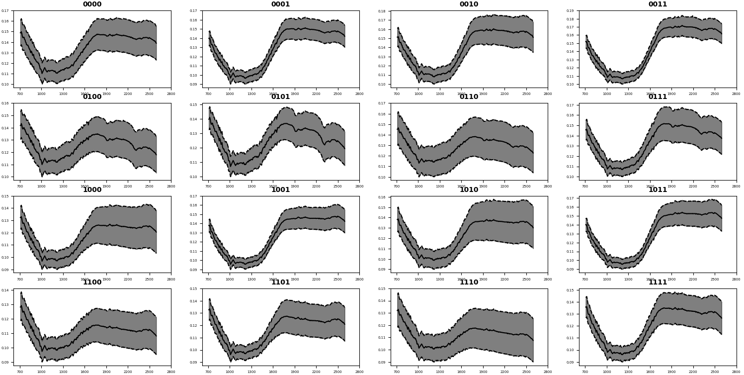
respectively (see figure 3 top left and bottom right). Finally, from each class, we extracted the
mean spectra and its standard deviation.

Table 1 and figure 1 reports the final model resulting from the random search hyperparameters
optimization process. Also, Figures 2 and 3 shows its application to the reflectance-deficient CRISM spectral parameter datacube. Figures 2 and 3 highlight that each pixel in the CRISM
datacube activates different neurons (Fig 2) and neuron combinations (Fig 3) in the latent space.
Figure 4 reports the superimposition of the different unique neuron combinations reported in
figure 3. In figure 4 b, each color represent a class of activated neurons and permits a more
direct comparison between the model’s extracted information and the morphological/albedo
features of the CRISM scenario (a). Figure 5 reports the mean spectra extracted for each
neuron combination that could be used for further investigations or for the comparison with
laboratory investigations.

Overall, we highlighted that undercomplete autoencoders could be a possible reliable instrument
for the analyses of hyperspectral datacube, from simple spectra extraction by clustering to the
generation of synthetic spectral parameters.

 

 

table 1

L. Rate	Enc. N.	Dec. N.	W. Decay	Enc. Dim.	Act.func.
0.05	25,15	45	0.0001	4	SiLU

 

figure 1

 

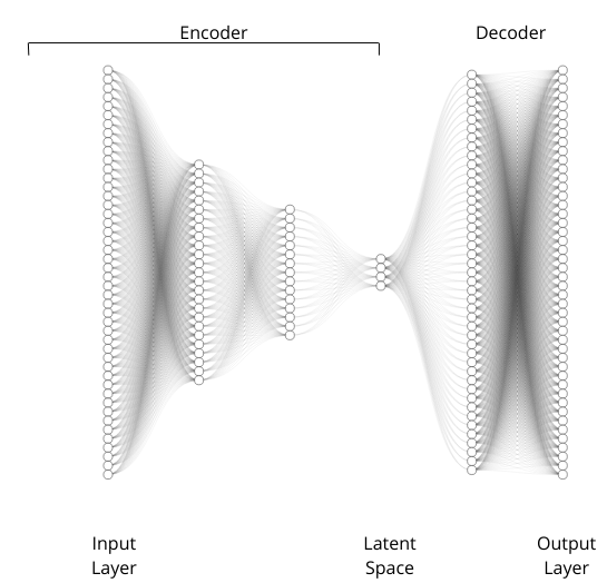
figure 2

 

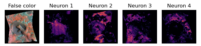
figure 3

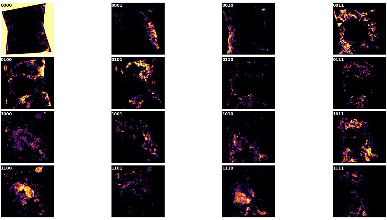
figure 4

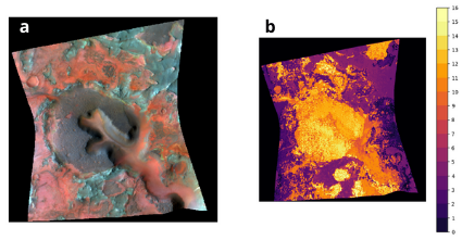
figure 5

[1] Murchie2007,E05S03

[2]Seelos2016,LPSCXXXXVII

[3]Viviano-Beck2014,119(6):1403-1431

[4]Baschetti2024,XIXCongressoNazionalediScienzePlanetarie

[5]Mustard2009,doi:10.1029/2009JE003349.

[6]Elhmann2008,Science,322,1228-1832

[7]Mustard2008,https://doi.org/10.1038/nature07097
https://doi.org/10.1038/nature07097