Multiple terms: term1 term2
red apples
returns results with all terms like:
Fructose levels in red and green apples
Precise match in quotes: "term1 term2"
"red apples"
returns results matching exactly like:
Anthocyanin biosynthesis in red apples
Exclude a term with -: term1 -term2
apples -red
returns results containing apples but not red:
Malic acid in green apples
hits for "" in
Network problems
Server timeout
Invalid search term
Too many requests
MITM3
Session assets
The application of machine learning techniques in astronomy has been rapidly growing, addressing various challenges such as predicting orbital stability, classifying celestial objects, and analysing images. However, the emerging trend of using large language models (LLMs) presents a novel approach that relies on natural language processing and explicit task definitions, rather than on statistical algorithms or probabilistic models. In this talk, I'll demonstrate the exceptional capabilities of LLMs, specifically GPT-4 as well as some other open source alternatives, in analyzing visual patterns and accurately classifying asteroids as resonant or non-resonant without any training, fine-tuning, or coding beyond writing an appropriate prompt in natural language. By leveraging the power of LLMs, it is possible to achieve an accuracy, precision, and recall of 100% in differentiating between pure libration, circulation, and mixed (transient) cases of resonant angles.
This approach introduces a new paradigm in astronomical data analysis, where complex tasks requiring human expertise can be completed with minimal effort and resources. The implications of this study extend beyond the identification of mean-motion resonances, as the methodology can be applied to a wide range of astronomical problems that involve pattern recognition, outlier detection, and decision-making tasks. This presentation will discuss the experimental design, results, and potential applications of LLMs in astronomy, highlighting the significance of this innovative approach in advancing astronomical research.
How to cite: Smirnov, E.: Effortless and accurate time series analysis in astronomy using Large Language Models, Europlanet Science Congress 2024, Berlin, Germany, 8–13 Sep 2024, EPSC2024-11, https://doi.org/10.5194/epsc2024-11, 2024.
Prompt Patterns provide general and reusable solutions to commonly occurring problems within specific contexts while interacting with a Large Language Model (LLM) such as GPT4. A catalog of generic prompt engineering patterns [1] has been published to help users improve LLM results and to promote further research into prompt engineering. Software engineering software patterns are an analog to prompt patterns, providing reusable solutions to common problems in a particular context.
The catalog defines six categories of prompt patterns including Input Semantics, Output Customization, Error Identification, Prompt Improvement, Interaction, and Context Control. Prompt patterns from two of the categories, Input Semantics and Output Customization have been applied to problems found in information modeling for the Planetary Data System (PDS).
How to cite: Hughes, J., Padams, J., Deen, R., and Joyner, R.: Prompt Patterns For PDS4 Information Modeling, Europlanet Science Congress 2024, Berlin, Germany, 8–13 Sep 2024, EPSC2024-76, https://doi.org/10.5194/epsc2024-76, 2024.
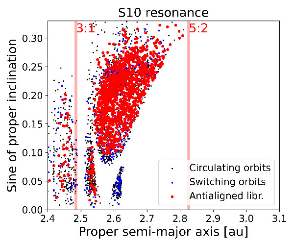
Node secular resonances, or s-type secular resonances, occur when the precession frequencies of the node of an asteroid and some planets are commensurable. They are important for changing the proper inclination of asteroids interacting with them. Traditionally, identifying an asteroid's resonant status was mostly performed by visually inspecting plots of the time series of the asteroid resonant argument to check for oscillations around an equilibrium point. More recently, deep learning methods based on convolutional neural networks (CNN) for the automatic classification of images have become more popular for these kinds of tasks, allowing for the classification of thousands of orbits in a few minutes. Convolutional layers are the main component of CNNs. They apply a set of learnable filters, or convolutional kernels, to the input tensor. Each filter is a small matrix that slides over the input tensor, performing element-wise multiplication and summing the results to produce a single value. Examples of CNN models are the Visual Geometry Group (VGG) (Simonyan & Zisserman 2014), the inception (Szegedy et al. 2015), and ResNet (He et al. 2015) models. In this work, we study 11 s-type resonances in the asteroid main belt and the Hungaria region (Knežević, 2021), and focus on the four most diffusive ones. Table (1) displays these resonances in terms of their resonant frequencies and as a combination of the arguments of linear resonances. The suffix in the frequencies identify the perturbing planet, 5 for Jupiter, 6 for Saturn, etc. The linear ν16 resonance has a resonant argument s-s6.
|
Resonance Identification |
Res. Argument (frequencies) |
Res. Argument (linear resonances) |
|
S2 |
2 · s − s4 − s6 |
ν16 + ν14 |
|
S4 |
s − 2 · s6 + s7 − g6 + g8 |
2 · ν16 − ν17 + ν6 − ν8 |
|
S10 |
s − s6 − g5 + g6 |
ν16 + ν5 − ν6 |
|
S11 |
s − s6 − 2 · g5 + 2 · g6 |
ν16 + 2 · ν5 − 2 · ν6 |
Table (1): The most diffusive s-type secular resonances in the main belt, according to this study. We report the resonant argument regarding frequencies and combinations of linear secular resonances.
We selected asteroids more likely to interact with each given resonance because of their proper s values, and, by visual inspection of their resonant argument, we identified the asteroids whose resonant argument oscillated around an equilibrium point (“librating” orbits), circulates from 0o to 360o (“circulating” orbits) and alternated phases of circulation and libration (“switching” orbits). Since we are interested in secular effects, we can apply a low-pass filter in frequency domains, like the Butterworth filter (Butterworth 1930), to allow low-frequency signals to pass through while attenuating high-frequency signals. Examples of asteroids on circulating and librating orbits without (left panels) and with the low-pass filter (right panels) are shown in Figure (1).
 |
 |
 |
 |
Figure(1): The left panels display images of the osculating resonant argument of the s-s6+g6−g5 secular resonance, while the right panels do the same for the filtered arguments.
We then applied CNN models for databases of unfiltered and filtered elements and computed their efficiency using standard machine learning metrics such as accuracy, Precision, Recall, and F1-score. Data for the S10 resonance are summarized in Table (2) and shown in Figure (2). Our results show that CNN models for filtered images are much more effective than traditional models applied to images of osculating resonant arguments.
|
Model |
Accuracy (%) |
Precision (%) |
Recall (%) |
F1-score (%) |
|
VGG (U) |
72 |
61.5 |
80 |
69.5 |
|
VGG (F) |
92 |
86.4 |
95 |
90.5 |
|
Inception (U) |
74 |
63 |
85 |
72.3 |
|
Inception (F) |
98 |
95.2 |
100 |
97.6 |
|
ResNet (U) |
62 |
51.6 |
80 |
62.7 |
|
ResNet (F) |
90 |
90 |
90 |
90 |
Table (2): Classification in terms of accuracy, precision, recall, and F1-score for the results obtained by CNN models for samples of unfiltered (U) and filtered (F) images of the S10 resonant arguments.
 |
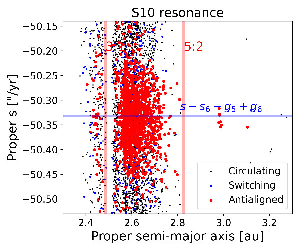 |
Figure (2): Proper (a,sin (i)) and (a,s) projections of numbered asteroids with errors in proper s < 0.2 arcsec yr−1 for bodies in the S10 resonance.
Filtered resonant arguments should be preferentially used to identify asteroids interacting with secular resonances. This work is currently under consideration by MNRAS.
References
Butterworth S., 1930, Wireless Engineer, 7, 536.
Carruba V., et al. 2021, CMDA, 133, 38.
Carruba V. et al. 2024, MNRAS, submitted.
He K., Zhang X., Ren S., Sun J., 2015, Deep Residual Learning for Image Recognition, doi:10.48550/ARXIV.1512.03385, https://arxiv.org/abs/1512.03385
Knežević Z., 2021, Serbian Academy of Sciences and Arts.
Lyapunov A. 1892, Annals of Mathematics and Mechanics, 17, 1.
Simonyan K., Zisserman A., 2014, arXiv e-prints, p. arXiv:1409.1556.
Szegedy C., et al., 2015, in Proceedings of the IEEE conference on computer vision and pattern recognition. pp 1–9.
How to cite: Carruba, V., Aljbaae, S., C. Domingos, R., Caritá, G., and Alves, A.: Deep learning classification of asteroids in s-type secular resonances, Europlanet Science Congress 2024, Berlin, Germany, 8–13 Sep 2024, EPSC2024-26, https://doi.org/10.5194/epsc2024-26, 2024.
1. Introduction
The advancement of computational techniques and methods such as artificial intelligence applied to celestial mechanics, including image classification. These techniques have been applied in the identification of mean motion resonances for asteroids (Smirnov and Markov, 2017; Carruba et al., 2021) and secular resonances for asteroids Carruba et al. (2022). The rapid growth of machine learning methods applications enables us to leverage these tools for the investigation of dynamical systems such as asteroid and planetary dynamics.
In the restricted three-body problem (R3BP), prograde orbits are those with an inclination less than 90 degrees with respect to the orbital plane of the perturber. Retrograde orbits are defined is this case with an inclination higher than 90 degrees (Morais and Namouni, 2017). These retrograde orbits can occur due to a range of astronomical events, such as collisions, close encounters and dissipation. This study aims to present a machine learning image classification method in order to search for periodic and quasi-periodic orbits, for example, retrograde orbits in the R3BP.
2. Resonances, resonant argument and perturbations
We establish the empirical case by defining μ ≤ 0.01, where μ is the mass ratio between the primaries. This threshold is determined after performing several tests involving different resonances. For values of 0.01 < μ < 0.3, there are only a few instances where the resonant argument can be reliably for identification. This observation could change based on the nature of the orbit. The chosen resonances for investigation are 1/-2, 2/-1, and 1/-1 (Morais and Namouni, 2013). The resonant argument (ϕ) in the Circular R3BP (CR3BP) is defined by ϕ = −pλp − qλ + (p + q)ϖ, where λ and λp are the respective longitudes of the massless and the secondary bodies, and ϖ represents the longitude of the pericenter of the massless body Morais and Namouni (2013). As an example we show the 2/-1 resonance presented in Figure 1, for μ = 0.02, we can still use the resonant argument as a way to identify this resonance, but we cannot determine only by the resonant argument whether it is the center of the resonant due to the amplitude. For μ = 0.1, the resonant argument cannot be analyzed for resonance identification.
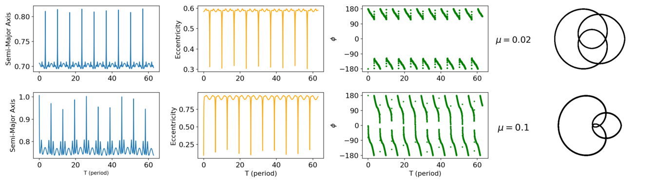
Figure (1): Examples of the osculating orbital elements and resonant argument for the resonance 2/-1.
In fact, when investigating families of periodic/quasi-periodic orbits using classical approaches, we could rely on the amplitude of the resonant argument and the libration mode for identification Caritá et al. (2022). For high mass ratio cases, this analysis could lead to partial results and misinterpretation.
3. Convolution Neural Network Model
A Convolutional Neural Network is a type of artificial neural network commonly used for image recognition and classification, emulating human abilities. The core concept involves building convolutional layers that apply filters, followed by a non-linear function to recognize image data patterns. In this study, we aim to identify resonant families by classifying mean motion resonances using their orbits (x, y) as an image parameter.
For the empirical problem of the planar CR3BP (PCR3BP) we considered the classes of the retrograde mean motion categorized as 1-1Phi0, 1-1Phi180, 1-2Phi0, 1-2Phi180, 2-1Phi0, 2-1Phi180, circular orbits and undefined. These classes represent resonances with libration at 0 or 180, and circular orbits. Figure 2 illustrates examples. Further details on the model parameters can be found in Caritá et al. (2024). As a validation benchmark, we obtained the 1/-2, 1/-1 and 2/-1 from Morais et al. (2021), Morais and Namouni (2019), and Kotoulas and Voyatzis (2020). The Figure 3 illustrates the output of the CNN prediction model successfully identifying circular, 1/-1, 1/-2, and 2/-1 resonant families.

Figure (2): Sample of the data used in the training.
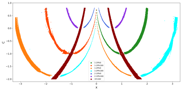
Figure (3): Classification of the resonances on the right panel.
4. Image resonance classification for high mass ratios in PCR3BP
As the mass of the binary body increases beyond the range of the empirical case, identifying resonances using Keplerian orbital elements becomes challenging due to the two-body problem approximations. However, resonances still exist in the phase space of the dynamical system, and they exhibit a behavior similar to that of empirical orbits in a rotating frame as seen in (Caritá et al., 2023). In Figure 4, the left panel presents the results obtained for a grid with μ = 0.5. The right panel shows the chaotic indicator (MEGNO). We observed a few gaps between some families. The orbits are different for high mass ratios. This could imply in difficulties identifying resonant families as μ increases.
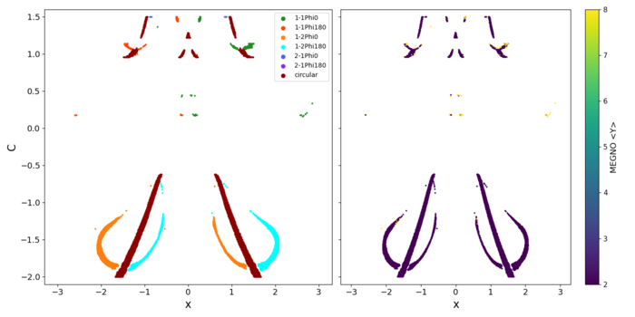
Figure (4): Classification of the resonances for the binary mass ratio of μ = 0.5.
5. Conclusions
The results obtained from the validation of our classification model demonstrate its effectiveness in accurately capturing the distinct patterns and characteristics of retrograde resonances. The model successfully identified retrograde resonances with high accuracy. The versatility of our classification model can extend beyond the constraints of the R3BP, making it adaptable to more intricate celestial environments. The model’s automated approach and efficiency offer researchers a potent tool for exploring a wide parameter space, quantifying stability, characterizing resonant behavior.
References
Smirnov, E.A., Markov, A.B.: MNRAS 469(2),2024-2031 (2017)
Carruba, V. et al, MNRAS, 504(1), 692–700 (2021)
Carruba , V. et al, MNRAS,514(4), 4803–4815 (2022)
Morais, M., Namouni, F., Nature 543(7647),635–636 (2017)
Morais, M., Namouni, F., CMDA, 117(4), 405–421 (2013)
Caritá, G.A et al MNRAS 515(2), 2280–2292 (2022)
Caritá, G.A et al CMDA 136(2), 1–24 (2024)
Morais, M., Namouni, F., CMDA, 133(5), 1-14 (2021)
Morais, M., Namouni, F., CMDA, 490(3), 3799-3805 (2019)
Kotoulas, T., Voyatzis, G., PSS, 182, 104846 (2020)
Caritá, G.A et al NODY 111(18), 17021-17035 (2023)
How to cite: Caritá, G., Aljbaae, S., Morais, M. H. M., Signor, A. C., Carruba, V., Prado, A. F. B. D. A., and Hussmann, H.: Image Classification of Retrograde Resonance in the Planar Circular Restricted Three-Body Problem, Europlanet Science Congress 2024, Berlin, Germany, 8–13 Sep 2024, EPSC2024-433, https://doi.org/10.5194/epsc2024-433, 2024.
Remote-sensing spectroscopy is the most efficient observational technique to characterise the surface composition of asteroids within a reasonable timeframe. While photometry allows to characterise much fainter targets, the resolution of characteristic absorption features via spectroscopy makes this technique the method of choice for many analysis avenues. The main contributors to our spectral database of asteroids have been large surveys, such as ECAS (Eight Color Asteroid Survey, [1]), SMASS (Small Main-Belt Asteroid Spectroscopic Survey, [2]), PRIMASS (PRIMitive Asteroids Spectroscopic Survey, [3]), MITHNEOS (MIT-Hawaii Near-Earth Object Spectroscopic Survey, [4]), and ESA Gaia. A significant number of observations has further been produced by individual efforts, focusing e.g. on asteroid families (e.g. [5, 6], among many others) and particular populations (e.g. [7, 8, 9], among many others). Currently, the number of visible / near-infrared / mid-infrared remote-sensing spectra of asteroids is around 70,000. This number will increase significantly in the years to come thanks to Gaia DR4 (expected in 2026) and the SPHEREx survey (to be launched in 2025, [10]). This is a positive development for the minor body community, and it has been recognised that, as the number of spectra continues to increase, we will require more sophisticated analysis methods to make best use of it. Numerous efforts have been undertaken to exploit these datasets with modern statistical treatment, for example, to identify clusters of asteroids (taxomic classes, [11, 12, 13, 14]), to invesitage asteroid-meteorite relationships ([15, 16, 17]), and for mineralogical characterization ([18, 19]). The recent strong increase in the number of asteroids with an observed spectrum further enables the independent confirmation of results obtained with other observables with literature spectra (e.g. asteroid families from dynamical elements, [20]).
A necessary prior step for all aforementioned analyses is the collection of public spectra from survey databases for the targets under investigation. These databases include NASA’s Planetary Data System, the Centre de Données astronomiques de Strasbourg, and online repositories of Gaia, SMASS, and MITHNEOS. Achieving a complete literature look-up for any given target is therefore a tedious task, given the large number of repositories and the heterogeneous datasets, in particular when accounting for smaller repositories based on the individual observational efforts referenced above. With an increasing number of spectra, this effort will increase. Two effects are visible: (1) Authors tend to visit one or two repositories and use an incomplete subset of the available spectra of a given asteroid. This hurts the scope of the analysis and therefore the results, as it is known that asteroid spectra can be subject to intrinsic (e.g. activity, [21]) and extrinsic (e.g. phase colouring, [22]) variability. (2) Important information like the metadata (for example, the epoch of observations and therefore phase angle of target) is commonly neglected in large-scale analyses given the large effort required to extract it.
The community could therefore benefit from a data-aggregator service focused on asteroid spectra. The classy tool aims to fill this gap by directly addressing the issue of accessibility of asteroid spectra. It itself is the product of a large, dedicated effort to build and homogenise a database of asteroid spectra, in preparation for a machine-learning appication to derive an asteroid taxonomy [12]. There are two main uses cases that classy aims to solve: (1) Search for and access of asteroid spectral observations based on properties of the spectra and the targets (e.g. retrieve all NIR spectra of asteroids in the Themis family with albedos < 0.05), and (2) to classify spectra in different taxonomic schemes (Tholen [23], Bus-DeMeo [11], Mahlke [12]). In addition, classy offers important functionality for common preprocessing of spectral data: truncating, interpolating, smoothing, and feature parameterisation. These preprocessing parameters are stored in a database that can be shared among users, supporting consistent data treatment among collaboration members and the publishing of reproducible results. Users can further ingest private observations into their local classy database to work in unison with public data. classy is connected to numerous online repositories of asteroid spectra, enabling to retrieve and query among approximately 70,000 spectra. A large effort was spent to extract the observational metadata from articles to allow studies to make use of the epoch of observation and the phase angle of the target. classy is a python package with a command-line interface and a web interface.1 It provides the important connection between repositories of spectra and users, greatly facilitating machine learning and other data-driven projects. It is actively developed, with a focus on stability and regarding the number of spectra that can be retrieved. Documentation is available online.2
1 https://classy.streamlit.app/
2 https://classy.readthedocs.io/
Acknowledgments: Without observations, there is not much to do. I thank all observers who choose to make their data available to the community.
Dr Benoit Carry provided important contributions to initial development of the classy database, in preparation of Mahlke et al. 2022.
References:
[1] Zellner, B. et al. (1985), Icarus, 61, 355-416
[2] Xu, S. et al. (1995), Icarus, 115, 1-35
[3] Pinilla-Alonso, N. et al. (2022), DPS, #504.09
[4] Binzel, R. et al. (2019), Icarus 324, 41-76
[5] Mothé-Diniz, T. and Carvano, J. M. (2005), A&A, 442, 727-729
[6] Marsset, M. et al. (2016), A&A, 586, A15
[7] Clark, B. E. et al. (2004), AAS, 128, 3070-3081
[8] de León, J. et al. (2012), Icarus, 218, 196-206
[9] Devogèle, M. et al. (2018), Icarus, 304, 31-57
[10] Ivezic, Z. et al. (2022), Icarus, 371, 114696
[11] DeMeo, F. et al. (2009), Icarus, 202, 160-180
[12] Mahlke, M. et al. (2022), A&A, 665, A26
[13] Penttilä, A. et al. (2022), A&A, 649, A46
[14] Klimczak, H. et al. (2022), A&A, 667, A10
[15] DeMeo, F. et al. (2022), Icarus, 380, 114971
[16] Mahlke, M. et al. (2023), A&A, 676, A94
[17] Galinier, M. et al. (2023), A&A, 671, A40
[18] Oszkiewicz, D. et al. (2022), MNRAS, 519, 2917-2928
[19] Korda, D. et al. (2023), A&A, 669, A101
[20] Carruba, V. et al. (2024), MNRAS, 528, 796-814
[21] Marsset, M. et al. (2019), ApJ Letters, 882, L2
[22] Alvarez-Candal, A. et al. (2024), A&A, 685, A29
[23] Tholen, D. (1984), PhD Thesis, MIT
How to cite: Mahlke, M.: Simplified access of asteroid spectral data and metadata using classy, Europlanet Science Congress 2024, Berlin, Germany, 8–13 Sep 2024, EPSC2024-172, https://doi.org/10.5194/epsc2024-172, 2024.
The aim of this work is to classify co-orbital motion at different timescales using a machine learning approach. Asteroids that move, on average, in a 1:1 mean motion resonance with a given planet, under the assumptions of the restricted three-body problem, are of special interest, because they follow very stable orbital configurations. The capability of classifying this kind of dynamics in an automatic way is of paramount importance to understand key mechanisms in the solar system but also for space exploration and exploitation missions. Starting from the analysis of Tadpole, Quasi-Satellite and Horseshoe regimes on a medium timescale, we apply features extraction and machine learning algorithms to the timeseries of the relative angle between the asteroid and the planet. The dataset is composed of pseudo-real timeseries computed by means of the JPL Horizons system (thus considering a full dynamical model) and simulated data computed by means of the REBOUND software. In a second step, the process is enriched to also be able to classify relative transitions between different co-orbital motions and between resonant and non-resonant dynamics, thus also considering much longer timescales. To this end, different algorithms are evaluated, starting from classical statistical approaches to more advanced deep learning ones.
How to cite: Azevedo, T., Ciacci, G., Di Ruzza, S., Barucci, A., and Alessi, E. M.: Towards a machine learning classification model of asteroids' co-orbital regimes, Europlanet Science Congress 2024, Berlin, Germany, 8–13 Sep 2024, EPSC2024-274, https://doi.org/10.5194/epsc2024-274, 2024.
In this session, we will discuss the use of Machine Learning methods for the identification and localization of cometary activity for Solar System objects in ground and in space-based wide-field all-sky surveys. We will begin the chapter by discussing the challenges of identifying known and unknown active, extended Solar System objects in the presence of stellar-type sources and the application of classical pre-ML identification techniques and their limitations. We will then transition to the discussion of implementing ML techniques to address the challenge of extended object identification. We will finish with prospective future methods and the application to future surveys such as the Vera C. Rubin Observatory.
How to cite: Bolin, B.: Identification and Localization of Cometary Activityin Solar System Objects with Machine Learning, Europlanet Science Congress 2024, Berlin, Germany, 8–13 Sep 2024, EPSC2024-136, https://doi.org/10.5194/epsc2024-136, 2024.
The moon is the earth's only natural satellite and it has a huge impact on the earth. Many countries have carried out a large number of lunar exploration missions over the years. The Lunar Reconnaissance Orbiter (LRO) launched by the United States in 2009 carried seven scientific instrument payloads to comprehensively map the lunar terrain and explore lunar resources. The optical narrow-angle camera (NAC) captures, processes and transmits back a large amount of image data [1]. These optical image data are intuitive data for studying the moon. Due to the axial tilt and undulating terrain, there are many areas (i.e., permanently shadowed regions (PSRs)) near the lunar south pole and north pole that are never illuminated by sunlight, so the imaging quality of these areas is poor. As shown in Fig. 1, PSR images have low signal-to-noise ratio (SNR), poor visibility, and most of the content is obscured. However, PSR may contain important materials such as water-ice, which makes it critical to study PSR with images. How to use low-light image enhancement methods to obtain high-quality PSR images has become a major challenge in this field.
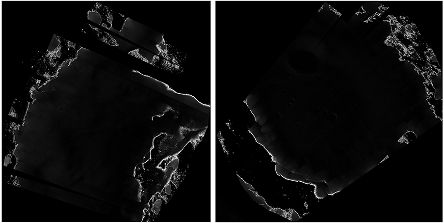
Fig. 1. Optical image examples of the lunar south pole PSR. These images were captured by LRO NAC and stitched together in post-processing.
Image enhancement is an important task in computer vision, which aims to design algorithms to improve the interpretability of images. Image enhancement in the past was mainly divided into traditional methods and deep learning methods. Traditional methods represented by histogram normalization (HE)[2] and dehazing model theory[3] are limited in enhancement range and physical assumptions, and have low automation capabilities. Deep learning methods are divided into supervised learning methods, GAN-based methods[4] and zero-shot learning methods. Supervised learning relies on pre-made paired datasets consisting of original and optimized images. However, for PSR images, there is no standard optimized image, so supervised learning methods are not suitable for PSR image enhancement. Although GAN-based methods get rid of the restrictions on paired datasets, they still need to select data to meet the needs of the generator and discriminator, which makes the process more cumbersome. The zero-shot learning method, which does not rely on any data and can directly enhance images, is suitable for the enhancement of scarce data such as PSR images. An important category of zero-shot learning methods is the decomposition of low-quality images derived from Retinex decomposition theory. Regarding an image G(x), Retinex theory believes that it can be divided into a combination of reflection map and illumination map, that is:
G(x) = R(x)•I(x)
where x is the pixel position of the image, R and I represent the reflection map and illumination map respectively. For low-light images such as PSR images, I(x) is too dark, and R, which represents image features, should also be adjusted. By adjusting these sub-maps, the Retinex-based method can achieve image enhancement.
However, traditional Retinex only considers the content and brightness of the image (i.e., reflectance map and illumination map), but does not consider image noise. Low-light images such as PSR have a low number of photons transmitted to the CCD during imaging, resulting in dim visual phenomena. But low photons not only reduce the brightness of the image, but also introduce a lot of noise, which further reduces the quality of the image. The traditional Retinex method will expand the original noise while adjusting the brightness, which hinders image content analysis. To this end, we propose a Retinex-based model RZSL-PSR that introduces noise estimation. This model decomposes the PSR image into reflection map, illumination map and noise map. The specific formula is:
G(x) = R(x)•I(x) + N(x)
Based on this formula, the model uses the proposed sub-map learning network to output three sub-maps respectively. The network structure includes downsampling, concatenation fusion, and skip connection structures, which helps to obtain feature maps that integrate multi-scale, strong semantic information, and high-resolution information.
Subsequently, the three output sub-maps are optimized to obtain the final output enhanced image. This process does not rely on learning image mappings of paired datasets, but instead utilizes a non-reference loss function to supervise model training. The loss function is as follows:
L = Lr + a•Lt + b•Ln
where Lr is the loss function to ensure that the output image conforms to the Retinex decomposition theory, Lt is the loss function to flatten the illumination uniformity of the image, and Ln is the loss function to estimate and suppress the noise in the dark area. Guided by these loss functions, the model learns nonlinear function mappings for enhancing PSR images, including increasing brightness and removing noise.
As shown in Fig. 2, the enhanced PSR image has better visibility than the original image. However, in order to highlight the landforms within the area for research on landforms and materials, we use USM sharpening for processing. The sharpening map results in Fig. 2 show that the landforms inside the PSR are highlighted, which helps to count the internal landforms.
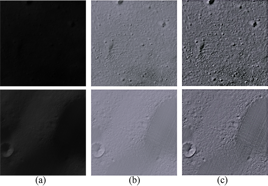
Fig. 2. PSR’s (original image)-(enhanced image)-(sharpened image) comparison example. Among them (a) is the input PSR image, (b) is the enhanced
image, and (c) is the image after USM sharpening of the enhanced image.
Acknowledgements
References
[1] Vondrak R, Keller J, Chin G, et al. Lunar Reconnaissance Orbiter (LRO): Observations for lunar exploration and science[J]. Space science reviews, 2010, 150: 7-22.
[2] Pisano E D, Zong S, Hemminger B M, et al. Contrast limited adaptive histogram equalization image processing to improve the detection of simulated spiculations in dense mammograms[J]. Journal of Digital imaging, 1998, 11: 193-200.
[3] Dong X, Pang Y, Wen J. Fast efficient algorithm for enhancement of low lightingvideo[M]//ACM SIGGRApH 2010 posters. 2010: 1-1.
[4] Meng Y, Kong D, Zhu Z, et al. From night to day: GANs based low quality image enhancement[J]. Neural Processing Letters, 2019, 50: 799-814.
How to cite: Zhang, F., Ye, M., Hao, W., Chen, Y., and Li, F.: A Retinex-based zero-shot learning method for permanently shadowed regions’ image enhancement, Europlanet Science Congress 2024, Berlin, Germany, 8–13 Sep 2024, EPSC2024-60, https://doi.org/10.5194/epsc2024-60, 2024.
From Pixels to Craters: Advancing Planetary Surface Analysis with Deep Learning.
La Grassa, R., Martellato, E., Re, C., Tullo, A., Vergara Sassarini, N.A. and Cremonese, G.
National Institute for Astrophysics (INAF), 35100 Padua, Italy
Introduction:
Over time, space missions with dedicated instruments for remote sensing allowed us to realize more and more accurate crater catalogs. Such catalogs are important tools for surface analysis. Given impact been collected continuously with time, they permit for instance to compare the different evolution of regions. In particular, when their size-frequency distribution is evaluated in conjunction with chronological models, craters allow datation of planetary surfaces, and provide insights into its geological evolution. In addition, when available both diameter and depth values of craters, the statistical analysis of structures can also provide geomechanical properties of the surface.
In this study, we present a comprehensive catalog of lunar impact craters, augmented by advancements in deep learning technology. This catalog is the final output of an articulated workflow that includes image pre-processing steps, application of an advanced double-architected neural network model, and final nested post-processing. This catalog not only extends the spatial resolution and coverage of existing databases (e.g., [3]), but also introduces a paradigm shift by including craters as small as 0.4 km in diameter. Moreover, the methodologies developed herein pave the way for the application of similar approaches to other celestial bodies, including for instance Mercury and the Ceres dwarf planet.
Catalog Overview:
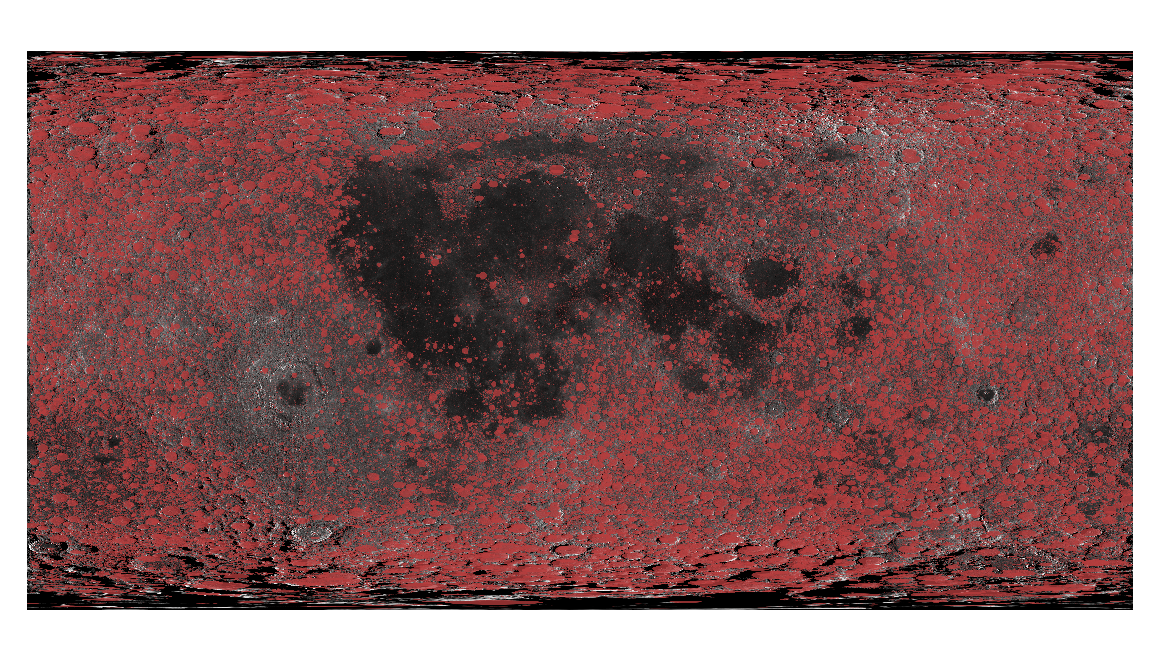
Our newly compiled catalog comprises approximately 5 million lunar impact craters (Fig. 2). Thanks to the implementation of a super-resolution algorithm, we were able to expand the lunar crater statistics down to 1 km in diameter, with nearly 69.3% of craters exhibiting diameters lower than 1 km. Furthermore, the impact craters detected in the 1-5 km and 5-100 km ranges are about 28.7% and 1.9% of the total catalog, respectively. Fig 2 shows the distribution of the extracted craters over the global basemap. The results in terms of Recall are very promising, as reported in Table 1, with performances varying with latitude.
|
|
|
Table 1: Number of tiles, Instances and Recall metric extracted by YOLOLens and different latitude degrees using Robbins Ground-Truth as main labels. |

Methodology and Validation:
Our approach exploits a custom neural network, refers as YOLOLens [1], which combines the principles of super-resolution with the state-of-the-art YOLO (You Only Look Once) object detection model [2]. This fusion of technologies enables the integration of high-resolution image processing with precise crater detection, yielding a comprehensive end-to-end solution for lunar crater cataloging. The methodologies developed for lunar crater detection are ready for adaptation and application to other celestial bodies, such as Mercury and the Ceres dwarf planet, expanding our understanding of impact cratering processes across the solar system.
To construct the YOLOLens model, we first enhanced the spatial resolution of lunar imagery, increasing the amount of detail available for crater identification. Subsequently, we integrated this enhanced imagery into the YOLO framework, allowing the localization of craters across the lunar surface. This innovative approach not only facilitated the detection of craters down to sizes as small as 0.4 km, but also ensured the accuracy and efficiency of the crater identification process.
Following the development of the YOLOLens model, extensive validation was conducted to assess its performance against established global crater catalogs. Through accurate comparisons and statistical analyses, we established a consistent crater size-frequency distribution for craters equal to or greater than 1 km, validating the efficacy of our methodology.
Elevation Data and Statistical Formulations:
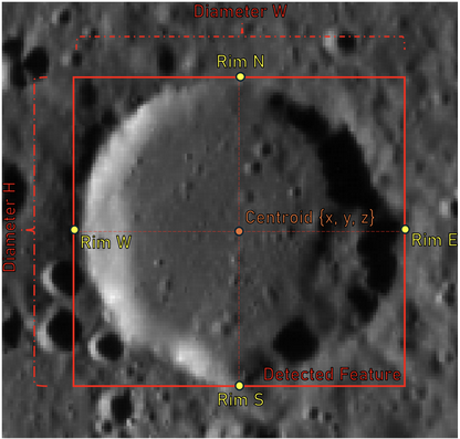
One additional characteristic of our catalog is that it provides not only the crater size and position, but also the elevation of the crater rims and center, facilitating a comprehensive analysis of lunar topography (Fig. 1). Moreover, we employ statistical formulations to extract essential crater parameters depth/diameter (d/D). The depth/diameter ratio, a fundamental measure in crater studies, holds particular importance in understanding the geological processes that shaped planetary surfaces. This ratio is a key indicator of crater formation mechanisms, impact energy, and surface properties, providing invaluable insights into planetary evolution. By incorporating elevation data and rigorous statistical analyses into our catalog, we empower researchers to improve the investigations on the lunar cratering processes.
This comprehensive approach not only enhances our understanding of lunar geology but also lays the groundwork for comparative studies across different planetary bodies. As such, the opportunity to provide elevation information and crater morphometric parameters underscores the comprehensive nature of our catalog and its significance in advancing planetary science research.
|
Figure 1: schematic representation of the 4 elevation rim extract by post-processing over the Lunar DTM using the bounding box predicted by YoloLens. The d/D measure and all elevations are introduced into the final catalog. |
|
Figure 2: Overview of the global catalog LU5M812TGT of ≥0.4 km lunar craters, highlighting craters with red circles on LROC WAC Global Mosaic |
Conclusion:
Through the integration of cutting-edge deep learning techniques and validation procedures, we constructed a complete global lunar catalog that offers an important resource for the understanding of lunar geology. This catalog stands to have an interdisciplinary collaboration and technological innovation in space exploration. Additionally, adapting our methodologies to other celestial bodies can further expand our knowledge of impact cratering processes and planetary evolution beyond the Moon.
References:
[1] La Grassa, R., Cremonese, G., Gallo, I., Re, C. and Martellato, E., 2023. YOLOLens: A deep learning model based on super-resolution to enhance the crater detection of the planetary surfaces. Remote Sensing.
[2] Redmon, J., Divvala, S., Girshick, R. and Farhadi, A., 2016. You only look once: Unified, real-time object detection. Computer vision and pattern recognition.
[3] Robbins, S.J., 2019. A new global database of lunar impact craters> 1–2 km: 1. Crater locations and sizes, comparisons with published databases, and global analysis. Journal of Geophysical Research.
Acknowledgements: we gratefully acknowledge funding from the Italian Space Agency (ASI) under ASI-INAF agreement 2017-47-H.0
How to cite: La Grassa, R., Martellato, E., Re, C., Tullo, A., Amanda, V. S., and Cremonese, G.: From Pixels to Craters: Advancing Planetary Surface Analysis with Deep Learning., Europlanet Science Congress 2024, Berlin, Germany, 8–13 Sep 2024, EPSC2024-390, https://doi.org/10.5194/epsc2024-390, 2024.
Introduction: Understanding the distribution and characteristics of impact craters on planetary surfaces is essential if we want to understand the geological processes such as tectonic deformation, volcanism1, erosion, transport, and impact cratering itself2 which constantly rebuilt planetary surfaces. By analysing the distribution and the density of crater using the "crater counting" approach, it is possible to estimate the age of the planetary surface3 at regional scale. Historically, crater detection has been made manually. For Mars and the Moon, the existing handmade databases4,5,6 brings an inestimable value to the community. Nevertheless, even with corrective analysis7, manual databases are subject to human limitations. Indeed, studies have shown that human attention to repetitive tasks, such as crater counting, rapidly decreases after 30 minutes8and then errors started to occur. Several machine learning and AI-based approaches have been proposed to automatically detect craters on planetary surface images9,10,11.
Data: To train our machine learning algorithm, we basically need two kind of data. We need images for the detection and a global crater database which encompass the ground truth. In this work we took images from the context camera on board of the Mars Reconnaissance Orbiter (CTX) and preprocess by the Bruce Murray Laboratory of Caltech12. For the crater database we took A. Lagain’s global martian database which encompass more than 376000 craters of a size bigger than 1 km in diameter7.
Method: In this work, we presents a novel approach using the Faster Region-based Convolutional Neural Network (Faster R-CNN) for automatic crater detection13. As shown in Fig. 1, Faster R-CNN employs three stages: CNN backbone extracts features, RPN generates ROIs with anchor boxes predicting object presence and adjustments, and Detector refines object classification and bounding box coordinates, ensuring precise object detection and localization in images.
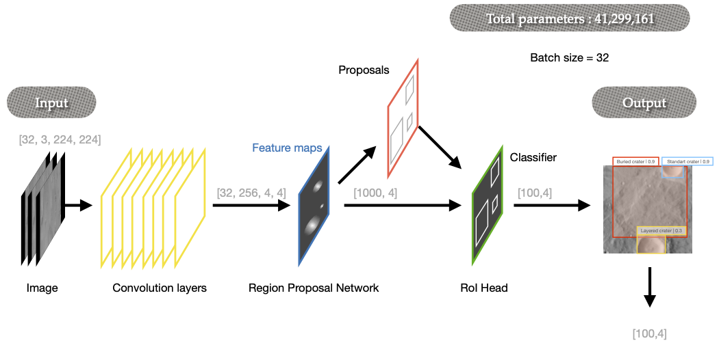
Fig. 1 : Faster R-CNN architecture as describe by S.Ren & al, 201613 with our image configuration
The proposed method involves a preprocessing step in which we cut the images to a size of 224x224 pixels, we reproject the images in order to be sure that crater will always have a circular shape at ever latitude and we split the crater database to have a ground truth label for each image. Then, we train our model with 82874 images and we test our detector on 4828 images.
Results: Extensive experiments on high-resolution planetary imagery demonstrate excellent performances with a mean average precision mAP50 > 0.82 with an intersection over union criterion IoU ≥ 0.5, independent of crater scale (Fig.2 & 3).
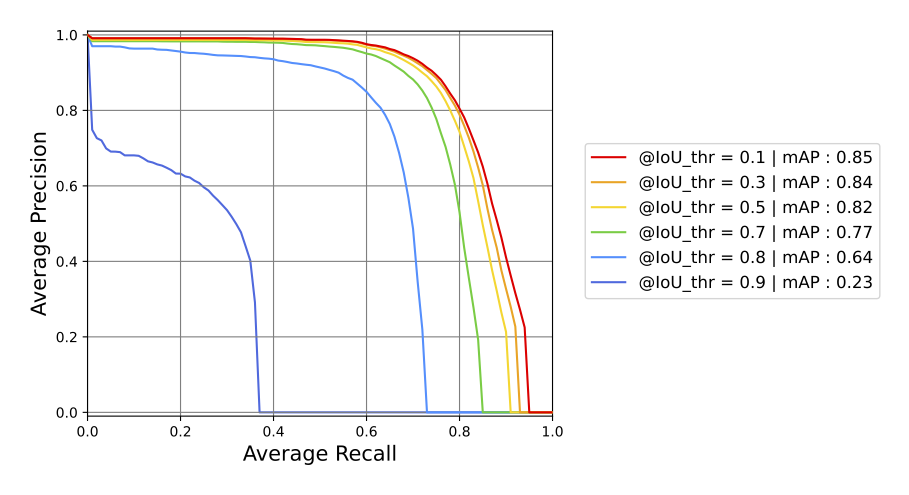
Fig. 2 : Precision as a function of recall for six different IoU thresholds.

Fig. 3 : Precision vs Recall curves for an IoU = 0.5 and for different bounding box sizes of the test dataset.
The Fig. 4 show an example on an equatorial Mars quadrangle.
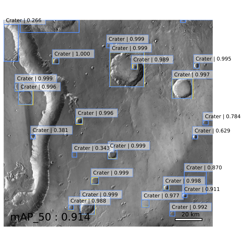
Fig. 4 : Inference on an equatorial region of Mars. The lower right corner of this 4°×4°
quadrangle is located at 44°W, 0°N. The yellow boxes represent the ground truth infor-
mation and the blue boxes the predictions ones. Please
note that crater smaller than 10 pixels in diameter are ignored.
The results also highlight the versatility and potential of our robust model for automating the analysis of craters across different celestial bodies. The automatic crater detection tool holds great promise for future scientific research of space exploration missions.
References:
[1] : M. H. Carr, Volcanism on mars 78 (20) 4049–4062. doi:10.1029/ jb078i020p04049.
[2] : Hartmann, William K., and Gerhard Neukum. "Cratering chronology and the evolution of Mars." Chronology and Evolution of Mars: Proceedings of an ISSI Workshop, 10–14 April 2000, Bern, Switzerland. Springer Netherlands, 2001.
[3] : G. Neukum, B. A. Ivanov, W. K. Hartmann, Cratering records in the in- ner solar system in relation to the lunar reference system, in: Chronology and Evolution of Mars: Proceedings of an ISSI Workshop, 10–14 April 2000, Bern, Switzerland, Springer, 2001, pp. 55–86.
[4] : Head III, James W., et al. "Global distribution of large lunar craters: Implications for resurfacing and impactor populations." science 329.5998 (2010): 1504-1507.
[5] : S. J. Robbins, A new global database of lunar impact craters¿ 1–2 km: 1. crater locations and sizes, comparisons with published databases, and global analysis, Journal of Geophysical Research: Planets 124 (4) (2019) 871–892
[6] : S. J. Robbins, B. M. Hynek, A new global database of mars impact craters ≥ 1 km: 1. database creation, properties, and parameters, Jour- nal of Geophysical Research: Planets 117 (E5) (2012).
[7] : A. Lagain, S. Bouley, D. Baratoux, C. Marmo, F. Costard, O. De- laa, A. P. Rossi, M. Minin, G. Benedix, M. Ciocco, et al., Mars crater database: A participative project for the classification of the morpho- logical characteristics of large martian craters, geoscienceworld (2021).
[8] : J. E. See, S. R. Howe, J. S. Warm, W. N. Dember, Meta-analysis of the sensitivity decrement in vigilance., Psychological bulletin 117 (2) (1995) 230.
[9] : Salamuniccar, Goran, and Sven Loncaric. "Method for crater detection from martian digital topography data using gradient value/orientation, morphometry, vote analysis, slip tuning, and calibration." IEEE transactions on Geoscience and Remote Sensing 48.5 (2010): 2317-2329.
[10] : G. Benedix, A. Lagain, K. Chai, S. Meka, S. Anderson, C. Norman, P. Bland, J. Paxman, M. Towner, T. Tan, Deriving surface ages on mars using automated crater counting, Earth and Space Science 7 (3) (2020) e2019EA001005.
[11] : R. La Grassa, G. Cremonese, I. Gallo, C. Re, E. Martellato, YOLOLens: A deep learning model based on super-resolution to enhance the crater detection of the planetary surfaces, Remote Sensing 15 (5) (2023) 1171. doi:10.3390/rs15051171.
[12] : Dickson, L.A.Kerber, C.I.Fassett, B.L.Ehlmann, A global, blended ctx mosaic of mars with vectorized seam mapping: a new mosaicking pipeline using principles of non-destructive image editing., 49th Lunar and Planetary Science Conference (2018).
[13] : S. Ren, K. He, R. Girshick, J. Sun, Faster r-cnn: Towards real-time object detection with region proposal networks (2016). arXiv:1506. 01497.
How to cite: Martinez, L., Schmidt, F., Andrieu, F., Bentley, M., and Talbot, H.: Automatic crater detection and classification using Faster R-CNN, Europlanet Science Congress 2024, Berlin, Germany, 8–13 Sep 2024, EPSC2024-1005, https://doi.org/10.5194/epsc2024-1005, 2024.
Introduction
Impact craters on the lunar surface are surrounded by boulders, rock fragments larger than 25.6 cm [1], which formed during the ejecta emplacement. These boulders are exposed on the surface and thus subject to meteoroid bombardment leading to two main erosional effects: abrasion and shattering [2]. Their abundance decreases with time producing regolith. By analyzing boulder fields, key information on regolith formation and evolution, as well as information about the subsurface rockiness of geologic units exposed by rock-excavating craters can be derived.
For this, global information of the distribution and size of boulders around impact craters is crucial. Currently, the only available global rock abundance map was derived with NASA’s Lunar Reconnaissance Orbiter (LRO) Diviner instrument [3] with an effective resolution of down to 330 m [4] but the dataset does not contain information about individual boulders. LRO Narrow Angle Camera (NAC) [5] images with resolutions of down to 0.5 m cover almost the entire lunar surface and are thus the best currently available source to map individual boulders on a global scale. For the vast majority of the more than 3 million available images, boulders have not been mapped. Compared to manual boulder counting, automated mapping of boulders allows for a substantially faster and reproducible analysis [e.g., 6-9].
Methods
Because of its great success in computer vision problems in various disciplines, we chose a deep learning approach for our boulder detection algorithm. Moreover, previous studies showed the feasibility to use deep learning for global mapping of the lunar surface [e.g., 10, 11]. Recently, we presented our boulder segmentation model [12], which utilizes Mask R-CNN [13] for a regional analysis with single NAC images. For the global analysis, we are now using the object detection model YOLOv8 [14, 15] to reduce the computational cost and required memory.
We utilize the publicly available calibrated pyramid tiff files of the LRO NAC images, which are reduced to 8bit but provide full spatial resolution. The model was trained with 512x512 pixel image tiles created from LRO NAC images displaying boulder fields and background. For all tiles, we manually mapped the boulders by creating a bounding box around the illuminated part. Currently, our dataset contains 12,000 mapped boulders with diameters > 2 m and 650 images.
Next, we applied the trained model to the lunar surface. As there is currently no global LRO NAC mosaic available, we developed an image selection algorithm. For each point on the lunar surface, from the NAC images covering that point, the one with the highest resolution is selected, while we only consider incidence angles between 35° and 75°. Each selected NAC image is then split into tiles and passed to the trained YOLO model for boulder detection.
Preliminary results
Currently, the model achieves an average precision of 65% with a precision of 66% and recall of 60% for the images of the validation set (Fig. 1). Most false negatives occur for small, likely highly abraded rocks with a reflectance that differs visually only slightly from the background regolith. False positives are mainly caused by outcrops whose boundaries cannot be clearly determined. The performance can be improved, e.g., by adding more examples of mapped boulders.
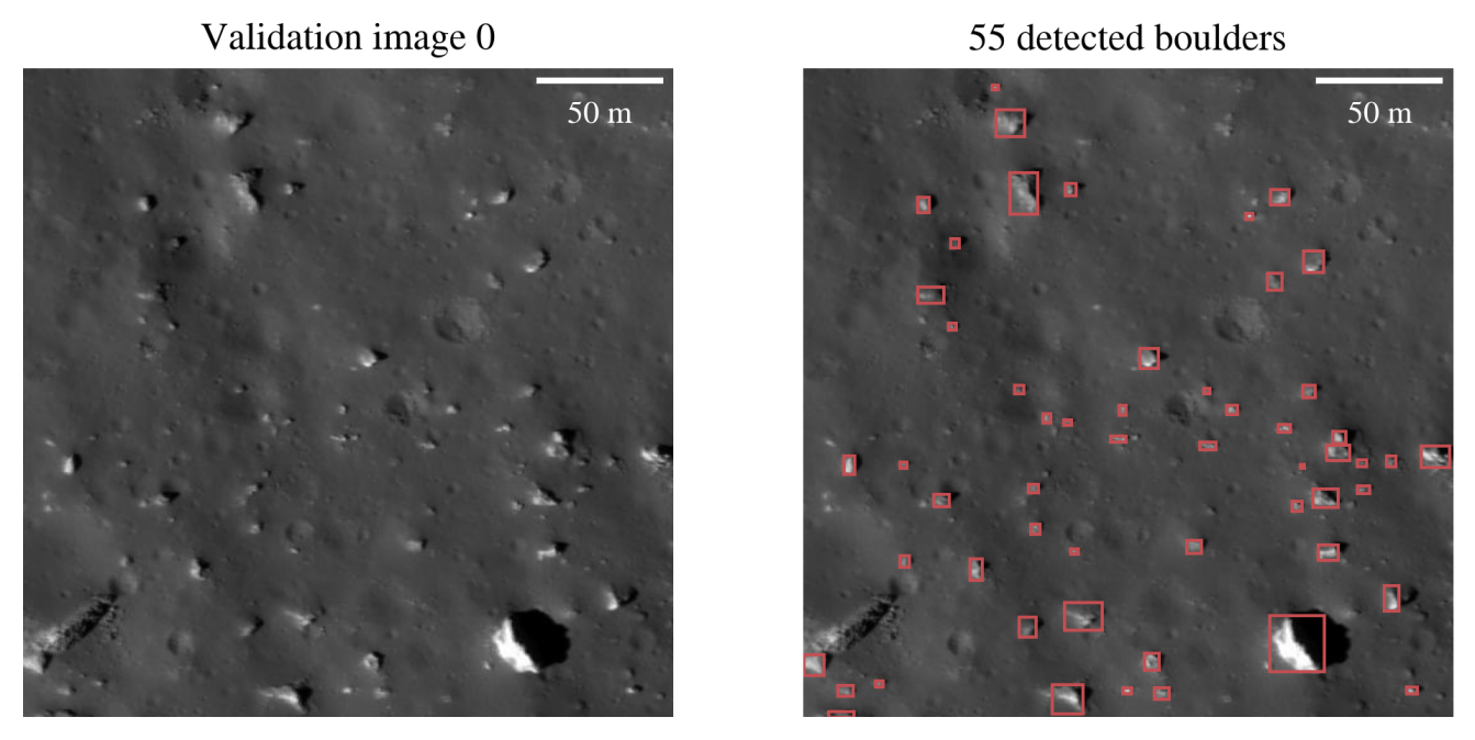
Figure 1: Examples of the detections (right) for a validation image (left, subframe of NAC image M112671946RC).
The model detects most boulders around impact craters correctly for regions that were not included in the training and validation process (Figs. 2 and 3). It can distinguish between background, particularly consisting of small craters, and boulders, which both display shadows. Boulders on crater walls remain mostly undetected, likely because of different lighting conditions currently not present in the training set and because of large shadows hiding boulders. Moreover, the specific lighting conditions for the utilized NAC images also influence the quality of the detections for boulders around craters, creating bands of differing absolute boulder abundances (Fig. 3). The mitigation of this effect is subject to current development.
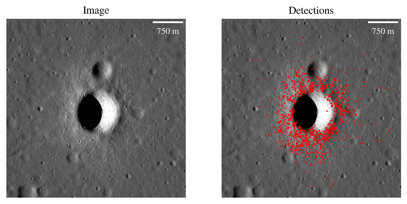
Figure 2: Examples of the detections (right) for a subframe of NAC image M193103501LC (left), which was not included in the training or validation set.
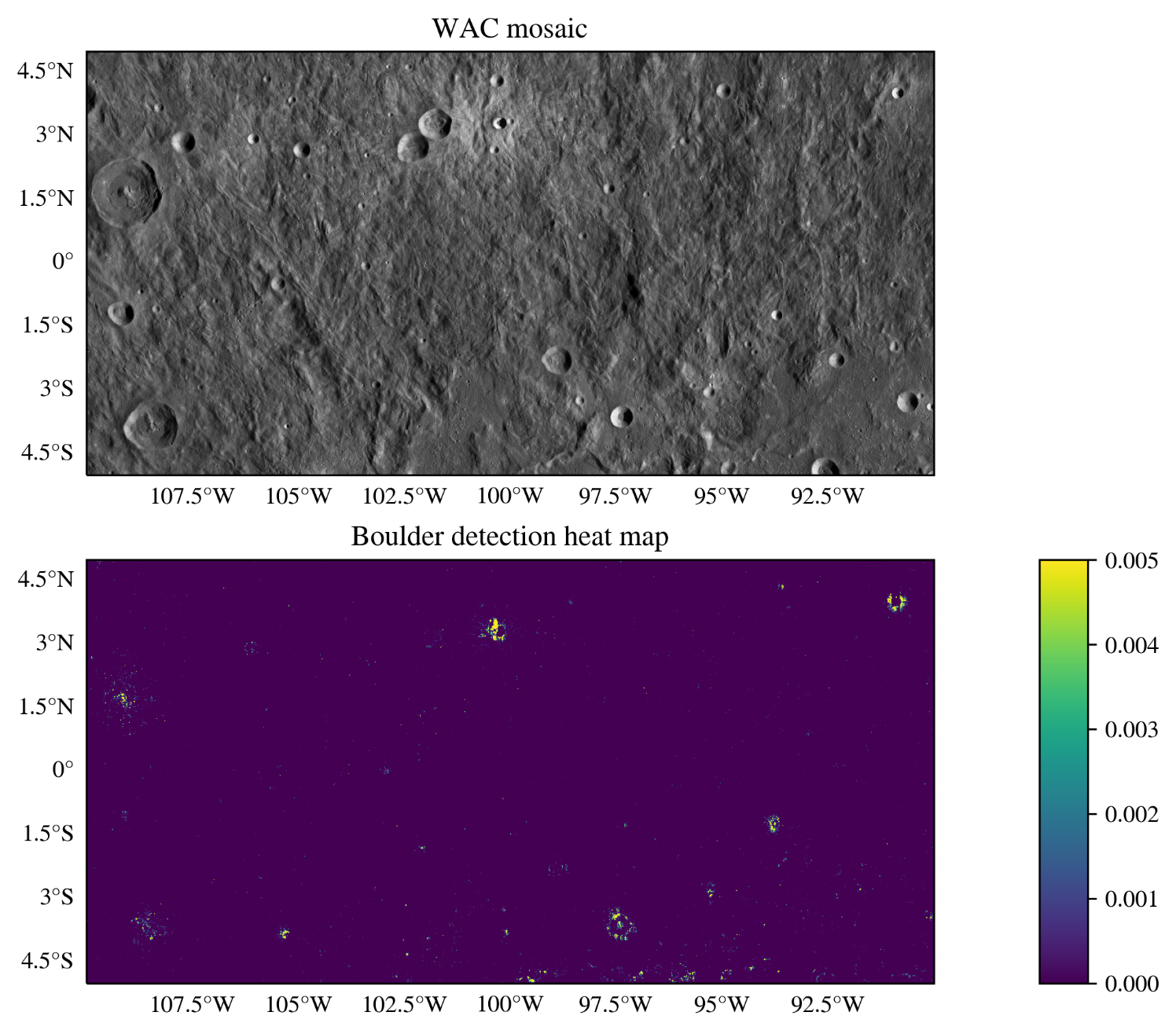
Figure 3: Example of a regional heat map of the boulder abundance (bottom), defined as the areal fraction of the detected boulders. For context, the publicly available mosaic, derived from LRO’s Wide Angle Camera [5] images, is shown for the same region (top).
Outlook
We are developing a deep learning model that can automatically map boulders in LRO NAC images, allowing for a reproducible analysis on a global scale. To improve the performance of the model and to minimize the effects of the specific illumination conditions, we plan to extend the training set. The model will then be used to derive a global map of boulders on the lunar surface to answer key questions about regolith formation and evolution and to improve thermophysical models of the lunar surface.
References
[1] Dutro J. T. J., Dietrich, R. V. and Foose, R. M. (1989), AGI data sheets for geology in the field, laboratory, and office.
[2] Hörz F. et al. (2020) PSS, 194, 105105.
[3] Paige D. A. et al. (2010) Space Sci. Rev., 150, 125-160.
[4] Powell T. M. et al. (2023) JGR : Planets, 128, e2022JE007532
[5] Robinson M. S. et al. (2010) Space Sci. Rev., 150, 81-124.
[6] Li Y. and Wu B. (2018) JGR : Planets, 123, 1061-1088.
[7] Bickel V. T. et al. (2019) IEEE Trans. Geosci. Remote Sens., 57, 3501-3511.
[8] Zhu L. et al. (2021) Remote Sens., 13, 3776.
[9] Prieur N. C. et al. (2023) JGR : Planets, 128, e2023JE008013.
[10] Bickel V. T. et al. (2020) Nat. Commun., 11, 2862.
[11] Rüsch O. and Bickel V. T. (2023), Planet. Sci. J., 4, 126.
[12] Aussel B. and Rüsch O. (2024) LPSC 55, Abstract #1834.
[13] He K. et al. (2017) Proc. IEEE Int. Conf. Comput. Vis., 2961-2969.
[14] Redmon J. et al. (2016) Proc. IEEE Comput. Soc. Conf. Comput. Vis. Pattern Recognit., 779-788
[15] Jocher G., et al. (2023) Github, Ultralytics YOLO (Version 8.0.0), https://github.com/ultralytics/ultralytics.
How to cite: Aussel, B., Rüsch, O., Gundlach, B., Bickel, V. T., Kruk, S., and Sefton-Nash, E.: Global mapping of boulders on the lunar surface with deep learning, Europlanet Science Congress 2024, Berlin, Germany, 8–13 Sep 2024, EPSC2024-998, https://doi.org/10.5194/epsc2024-998, 2024.
The detailed and accurate shape of the terrain is necessary for some fields, such as geodetic analysis and geomorphology, which are concerned with the physical processes of a planet and its orbital attitudes. The Mercury Laser Altimeter (MLA) onboard the MESSENGER orbiter has performed successive altimetry measurements between 2011 and 2015. These measurements provide a global shape of the planet with approximately 3200 laser profiles, with the majority of these profiles covering the northern hemisphere due to MESSENGER's highly elliptical orbit (Cavanaugh et al., 2007). A number of studies have sought to derive digital terrain models (DTMs) of Mercury using stereo-imaging techniques (Fassett, 2016; Manheim et al., 2022, Florinsky, 2018). Some have employed MLA data (Zuber et al., 2012; Preusker et al., 2017). However, challenges remain due to discrepancies in the laser altimeter tracks, which are thought to be due to residual errors in spacecraft orbit, pointing, etc. Filtering these offsets provides an opportunity for further refinement and improvement of DTM generation methods for Mercury's surface.
The aim of this paper is to accurately extract terrain from MLA point clouds, particularly around the characteristic features of the northern hemisphere, at high resolutions. In this work, we propose an algorithm that follows a region-growing approach to extract the terrain. To identify the optimal surface solution in each local patch (Arghavanian, 2022), we apply machine learning methods and statistical parameters, starting from regions that are relatively easy to fit and then growing to the most challenging areas. Additionally, users have the flexibility to add or remove constraints or fine-tune terrain-relevant and empirical parameters based on their specific topography. The final surface is obtained by global surface fitting, thereby filling any gaps in the data. To evaluate the performance of the proposed method, the results will be compared with previously produced DEMs.
References:
Arghavanian A., 2022, Channel detection and tracking from LiDAR data in complicated terrain, PhD thesis, Middle East Technical University, Ankara, Turkey.
Cavanaugh, J.F. et al. (2007) ‘The Mercury Laser Altimeter Instrument for the MESSENGER Mission’, Space Science Reviews, 131(1), pp. 451–479. Available at: https://doi.org/10.1007/s11214-007-9273-4.
Fassett C.I., 2016, Ames stereo pipeline-derived digital terrain models of Mercury from MESSENGER stereo imaging, Planetary and Space Science, Volume 134, Pages 19-28.
Florinsky I.V., 2018, Multiscale geomorphometric modeling of Mercury, Planetary and Space Science Volume 151, Pages 56-70.
Manheim M.R., Henriksen M.R., Robinson M.S., Kerner H. R., Karas B.A., Becker K.J., Chojnacki M., Sutton S.S., Blewett D.T., 2022, High-Resolution Regional Digital Elevation Models and Derived Products from MESSENGER MDIS Images, Remote Sens, 14, 3564.
Preusker F, Stark A, Oberst J, Matz K.D., Gwinner K, Roatsch T, Watters T.R., 2017, Planetary and Space Science, Volume 142, Pages 26-37.
Zuber, M.T. et al. (2012) ‘Topography of the Northern Hemisphere of Mercury from MESSENGER Laser Altimetry’, Science, 336(6078), pp. 217–220. Available at: https://doi.org/10.1126/science.1218805.
How to cite: Arghavanian, A., Stenzel, O., and Hilchenbach, M.: Smooth Hermean surface extraction by Region Growing from MESSENGER Laser Altimeter Data , Europlanet Science Congress 2024, Berlin, Germany, 8–13 Sep 2024, EPSC2024-320, https://doi.org/10.5194/epsc2024-320, 2024.
This work introduces an approach to enhance the computational efficiency of 3D Global Circulation Model (GCM) simulations by integrating a machine-learned surrogate model into the OASIS GCM[1]. Traditional GCMs, which are based on repeatedly numerically integrating physical equations governing atmospheric processes across a series of time-steps, are time-intensive, leading to compromises in spatial and temporal resolution of simulations. This research improves upon this limitation, enabling higher resolution simulations within practical timeframes.
Speeding up 3D simulations holds significant implications in multiple domains. Firstly, it facilitates the integration of 3D models into exoplanet inference pipelines, allowing for robust characterisation of exoplanets from a previously unseen wealth of data anticipated from post-JWST instruments[2-3]. Secondly, acceleration of 3D models will enable higher resolution atmospheric simulations of Earth and Solar System planets, enabling more detailed insights into their atmospheric physics and chemistry.
This work builds upon previous efforts in both exoplanet science and Earth climate science to accelerate 3D atmospheric models. Prior work in exoplanet science primarily relies on extrapolating 1D models to approximate certain 3D atmospheric variations[4-6], which often introduces both known and unknown biases. Earth climate science, benefiting from a wealth of high-resolution observational measurements, has had a different set of methods employed, namely machine-learned surrogate models trained on such observations[7-8]. This work employs machine-learned surrogate model techniques, benchmarked in Earth climate science[8], to be used in general planetary climate models.
Our method replaces the radiative transfer module in OASIS with a recurrent neural network-based model trained on simulation inputs and outputs. Radiative transfer is typically one of the slowest and lowest resolution components of a GCM, thus providing the largest scope for overall model speed-up. The surrogate model was trained and tested on the specific test case of the Venusian atmosphere, to benchmark the utility of this approach in the case of non-terrestrial atmospheres. This approach yields promising results, with the surrogate-integrated GCM demonstrating above 99.0% accuracy and 10 times CPU speed-up compared to the original GCM.
In conclusion, this work presents a method to accelerate 3D GCM simulations, offering a pathway to more efficient and detailed modelling of planetary atmospheres.
References:
[1] Mendonca J. & Buchhave L., ‘Modelling the 3D Climate of Venus with OASIS’, 2020, Volume 496, Pages 3512-3530, Monthly Notices of the Royal Astronomical Society
[2] Gardner, J. P., “The James Webb Space Telescope”, Space Science Reviews, vol. 123, no. 4, pp. 485–606, 2006. doi:10.1007/s11214-006-8315-7.
[3] Tinetti, G., “Ariel: Enabling planetary science across light-years”, arXiv e-prints, 2021. doi:10.48550/arXiv.2104.04824.
[4] Q. Changeat and A. Al-Refaie, “TauREx3 PhaseCurve: A 1.5D Model for Phase-curve Description,” Astrophys J, vol. 898, no. 2, p. 155, Aug. 2020, doi: 10.3847/1538-4357/ab9b82.
[5] K. L. Chubb and M. Min, “Exoplanet atmosphere retrievals in 3D using phase curve data with ARCiS: application to WASP-43b,” Jun. 2022, doi: 10.1051/0004-6361/202142800.
[6] P. G. J. Irwin et al., “2.5D retrieval of atmospheric properties from exoplanet phase curves: Application toWASP-43b observations,” Mon Not R Astron Soc, vol. 493, no. 1, pp. 106–125, Mar. 2020, doi: 10.1093/mnras/staa238.
[7] Yao, Y., Zhong, X., Zheng, Y., & Wang, Z. 2023, Journal of Advances in Modeling Earth Systems, 15, e2022MS003445, doi: 10.1029/2022MS003445
[8] Ukkonen, P. 2022, Journal of Advances in Modeling Earth Systems, 14, e2021MS002875, doi: 10.1029/2021MS002875
How to cite: Tahseen, T., Mendonça, J., and Waldmann, I.: Accelerating Radiative Transfer in 3D Simulations of the Venusian Atmosphere, Europlanet Science Congress 2024, Berlin, Germany, 8–13 Sep 2024, EPSC2024-356, https://doi.org/10.5194/epsc2024-356, 2024.
1. Introduction
When working with atmospheric data, researchers often face partial datasets. This is the case of the SOIR instrument on board Venus Express [1], which measured the temperature of the Venus mesosphere, inferred via solar occultations. Due to inherent limitations in the measurement process, temperature measurements are missing at varying altitudes in the profiles. While altitudes of measurements across the whole dataset can span from 60 km to 160 km, most of the profiles only contain a range of 10 to 50 consecutive measurements. Figure 1 shows examples of such profiles. To fill this data gap, machine learning, and specifically probabilistic models are promising candidates.
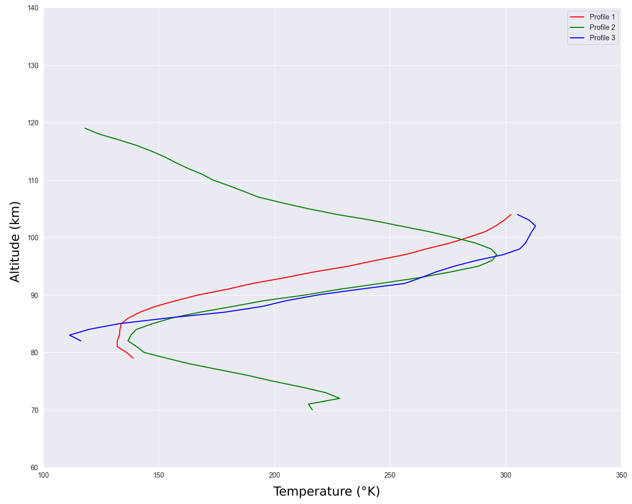
Fig. 1: Three temperature profiles from SOIR, with varying ranges of altitude.
2. Gaussian Processes and MAGMA
Gaussian processes (GPs) are probabilistic models mainly used for predictions based on empirical observations. The capacity of GPs to estimate the uncertainty in their predictions makes them particularly appropriate for extrapolating atmospheric data. Since traditional GPs only try to fit a single function, adaptations should be implemented for the case of the SOIR dataset, which contains numerous profiles. Using one GP for each profile would not allow models to leverage information across the whole dataset to make better predictions. This motivates the use of so-called multi-task GPs, where “task” refers to an atmospheric profile in our context. The literature in the field of multi-task GPs is extensive [2, 3, 4], but most models either struggle with large datasets or have difficulties learning the covariance between the tasks. The MAGMA algorithm [5] is a recent advancement in the field of multi-task GPs that solves the above-mentioned issues. To complete a gap at a specific altitude in a profile, MAGMA uses both the profile values that are close to the gap and the mean value measured at that altitude in all other profiles. This results in better confidence intervals, even far from known observations. Previous to this work, MAGMA had never been applied to atmospheric datasets.
3. Profile Extrapolation
To assess the performances of MAGMA, we compare this algorithm with a traditional GP working on each profile individually. First, each profile is preprocessed to standardise each temperature value and use a logarithmic pressure scale as a height indicator rather than altitude. As MAGMA needs profiles to share common inputs, each pressure measurement is mapped to its closest bin on a 250 discrete bin scale. We then divide the dataset into train and test sets. Each test profile is further divided into test observations and validation observations. During experiments, test observations are given to the models as a starting point. The models can then make predictions, providing an estimated mean value and a confidence interval for each missing pressure bin. The validation observations are compared with their corresponding predictions to evaluate the performances of each model. Experimental results show that MAGMA has significantly better performances than a traditional GP, as seen in Figure 2. It provides estimations that are closer to the actual measurement and confidence intervals that are more precise, as shown in Figure 3.
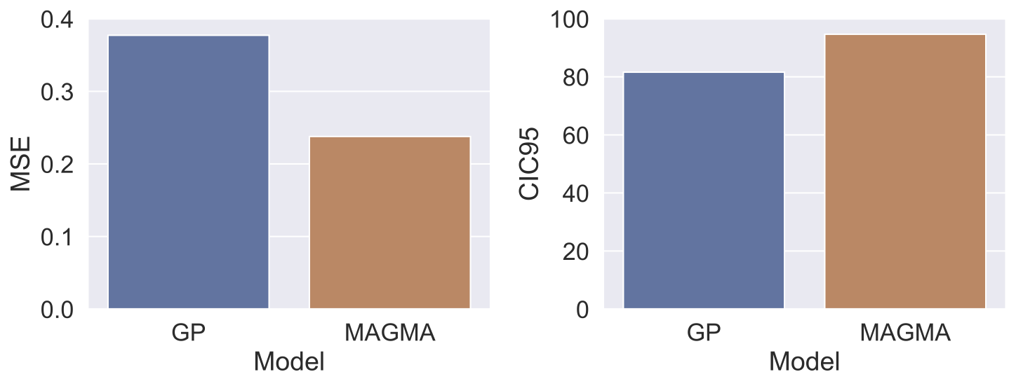
Fig. 2: Average performances of MAGMA and the baseline model on two distinct metrics. Mean Squared Error (MSE) measures the distance between predictions and true values (to be minimised). CIC95 is the ratio of validation observations actually sitting in the predicted 95% confidence interval (should be close to 95%).
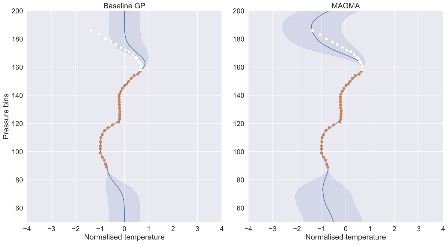
Fig. 3: Predictions from the baseline and MAGMA, for different training settings. The test observations and validation observations are represented in orange and white, respectively. The grey-shaded area corresponds to the 95% confidence interval.
4. Conclusion
We apply MAGMA, a novel probabilistic learning algorithm, to the SOIR dataset, enhancing predictions for missing observations. This contribution is a first step toward a practical application of GPs to planetary aeronomy datasets. Future research will explore possible enhancements to the data preprocessing and model architectures to complete the SOIR dataset with more precise and credible estimations.
References
-
[1] L. Trompet, Y. Geunes, T. Ooms, et al. Description, accessibility and usage of SOIR/Venus Express atmospheric profiles of Venus distributed in VESPA (Virtual European Solar and Planetary Access). Planetary and Space Science, 150:60–64, 2018.
-
[2] Edwin V Bonilla, Kian Chai, and Christopher Williams. Multi-task Gaussian Process Prediction. In Advances in Neural Information Processing Systems, volume 20, 2007.
-
[3] Edwin V. Bonilla, Felix V. Agakov, and Christopher K. I. Williams. Kernel Multi-task Learning using Task-specific Features. In Proceedings of the Eleventh International Conference on Artificial Intelligence and Statistics, pages 43–50. PMLR, 2007.
-
[4] Carlos Ruiz, Carlos M. Alaiz, and José R. Dorronsoro. A survey on kernel-based multi-task learning. Neurocomputing, 577:127255, 2024.
-
[5] Arthur Leroy, Pierre Latouche, Benjamin Guedj, and Servane Gey. MAGMA: inference and prediction using multi-task Gaussian processes with common mean. Machine Learning, 111(5):1821–1849, 2022.
How to cite: Lejoly, S., Piccialli, A., Mahieux, A., Vandaele, A. C., and Frénay, B.: MAGMA Gaussian Processes to complete Venusian atmospheric profiles from SOIR , Europlanet Science Congress 2024, Berlin, Germany, 8–13 Sep 2024, EPSC2024-382, https://doi.org/10.5194/epsc2024-382, 2024.
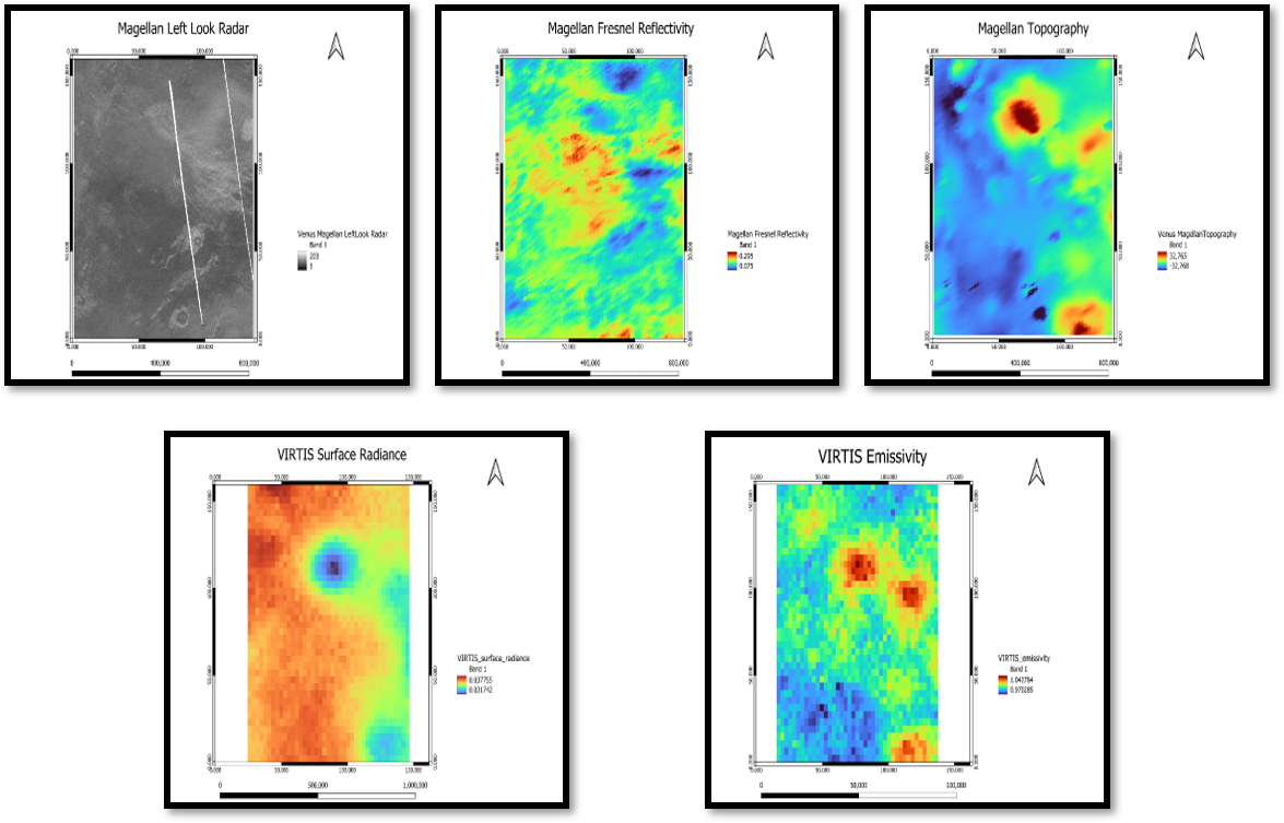 This study investigates the geological characteristics of the transition area between Themis Regio and Helen Planitia on Venus, leveraging a multi-layered dataset comprising Magellan Radar data, Magellan Fresnel Reflectivity, Magellan Topography, VIRTIS Surface Radiance and VIRTIS Emissivity. The selection of this region aligns with the standardized area utilized in the tutorials presented at the GMAP Winter School 2024, facilitating comparative analysis with established geological mapping methodologies. The data layers are meticulously stacked and subjected to comprehensive preprocessing procedures to ensure consistency and mitigate inherent challenges associated with Venusian remote sensing datasets, including atmospheric interference and topographical variations. Subsequently, unsupervised clustering techniques are employed to delineate meaningful spatial patterns within the dataset stack. In this investigation, we explore two widely recognized unsupervised clustering methodologies: K-means clustering and Self-Organizing Maps (SOM).
Notably, our analysis reveals that the SOM yields a less cluttered cluster map than the k-means algorithm within the Venusian dataset and appears to capture intricate geological features. Furthermore, the SOM yields a geologically reasonable scene segmentation also without the application of dimensionality reduction techniques such as Principal Component Analysis (PCA), suggesting its robustness in handling high-dimensional datasets inherent to planetary remote sensing. Moreover, beyond traditional clustering methodologies, our research is planned to extend towards supervised learning approaches utilizing the outputs of unsupervised clustering for automated feature identification. This hybrid methodology harnesses the strengths of both unsupervised and supervised learning paradigms, offering a comprehensive framework for geological mapping and feature characterization on planetary surfaces. The findings of this study contribute to advancing our understanding of Venusian geology and refining remote sensing methodologies tailored for planetary exploration. The insights garnered from this research are instrumental not only in unraveling the geological complexities of Venus but also in informing future missions and exploration endeavors aimed at unraveling the mysteries of our neighboring planet.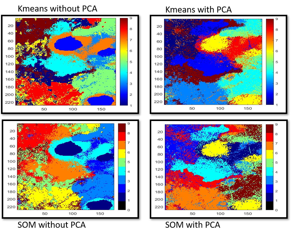
How to cite: Garg, S. and Woehler, C.: A Case Study of Classification Comparison of Venusian Data Layers for Geological Mapping, Europlanet Science Congress 2024, Berlin, Germany, 8–13 Sep 2024, EPSC2024-827, https://doi.org/10.5194/epsc2024-827, 2024.
Introduction
Mars’ dust cycle is a critical factor that drives the weather and climate of the planet. Airborne
dust affects the energy balance that drives the atmospheric dynamic. Therefore, for studying the present-day and recent-past climate of Mars we need to observe and understand the different processes involved in the dust cycle. To this end, the Mars Environmental Dynamics Analyser (MEDA) station [1] includes a set of sensors capable of measuring the radiance fluxes, the wind direction and velocity, the pressure, and the humidity over the Martian surface. Combining these observations with radiative transfer (RT) simulations, airborne dust particles can be detected and characterized (optical depth, particle size, refractive index) along the day. The retrieval of these dust properties allows us to analyze dust storms or dust-lifting events, such as dust devils, on Mars [2][3].
Dust devils are thought to account for 50% of the total dust budget, and they represent a
continuous source of lifted dust, active even outside the dust storms season. For these reasons, they have been proposed as the main mechanism able to sustain the ever-observed dust haze of the Martian atmosphere. Our radiative transfer simulations indicate that variations in the dust loading near the surface can be detected and characterized by MEDA radiance sensor RDS [4].
This study reanalyzes the dataset of dust devil detections obtained in [3] employing artificial
intelligence techniques including anomaly detection based on autoencoders [5] and deep learning models [6] to analyze RDS and pressure sensor data. As we will show, preliminary results indicate that our AI models can successfully identify and characterize these phenomena with high accuracy. The final aim is to develop a powerful tool that can improve the database for the following sols of the mission, and subsequently extend its use for other atmospheric studies.
Dataset
The dataset used in this study includes data from 365 Martian days, which represents half a Martian year of observations and it was collected with a temporal resolution of one sample per second (for 12 hours in average observations per sol). This dataset, which has been labeled by hand, contains 424 detected Dust Devil events. The duration of these events varies considerably, ranging from just a few seconds to several minutes. The precise manual labeling is crucial for training reliable machine learning models that can effectively recognize and predict these events.
AI techniques
Deep learning is increasingly used to detect events in time-based signals, significantly enhancing accuracy and speed. Methods like CNN [7] and RNN [8] identify complex patterns effectively. These models learn from vast data, enabling real-time and predictive analytics.
Deep learning-based autoencoders are powerful tools for anomaly detection in temporal signals [5], offering a sophisticated method to capture complex patterns and identify outliers. Autoencoders, which are neural networks designed to reconstruct their input, learn to represent normal patterns during training. By minimizing the reconstruction error, these models learn to encode the regular, predictable aspects of temporal data. When an anomalous signal occurs, it typically results in a higher reconstruction error due to deviations from learned patterns.
The nature of the events and the low frequency of occurrence presents two main challenges for the Machine Learning algorithm:
• The database is highly unbalance. As it is said in Section Dataset, 424 events are detected over 365 Martian days. It means that less than 0.2% of the database corresponds to Dust Devil cases.
• Due to the spatial nature of the events, the Dust Devils manifests in different RDS sensors each time. This makes it difficult for the algorithm to generalize.
Results
For the experiments, the data is windowed and data augmentation techniques are used to try to correct the issue of class imbalance. The training set was selected randomly and intentionally balanced to ensure an equal number of samples per class. For testing the models, data from six randomly chosen suns are selected. The following results (Table 1) are obtained:
| Name | Train Accuracy | Test Accuracy |
| DNN | 75.0% | 65.7% |
| CNN | 82.5% | 78.9% |
| LSTM | 73.1% | 67.0% |
At the time of writing this document, there are no consistent results for autoencoder’s approach.
Conclusions and Future Steps
This study demonstrates that data augmentation and advanced AI techniques can significantly improve the detection of dust devils on Mars. The use of deep learning, specifically convolutional neural networks (CNNs), has shown to outperform other models in accuracy both during training and testing phases.
Future work will focus on enhancing feature extraction, exploring new data augmentation techniques, and further developing autoencoders.
Acknowledgements
This work was funded by the Spanish Ministry of Science and Innovation under Project PID2021-129043OB-I00 (funded by MCIN/AEI/10.13039/501100011033/FEDER, EU), and by the Community of Madrid and University of Alcala under project EPU-INV/2020/003.
[1] Rodriguez-Manfredi at al. The mars environmental dynamics analyzer, meda. a suite of
environmental sensors for the mars 2020 mission. Space Science Reviews, 217, 04 2021.
[2] Lemmond et al. Dust, sand, and winds within an active martian storm in jezero crater. Geophysical Research Letters, 49(17):e2022GL100126, 2022. e2022GL100126 2022GL100126.
[3] Toledo et al. Dust devil frequency of occurrence and radiative effects at jezero crater, mars, as
measured by meda radiation and dust sensor (rds). Journal of Geophysical Research: Planets,
128(1):e2022JE007494, 2023. e2022JE007494 2022JE007494.
[4] Ap´estigue et al. Radiation and dust sensor for mars environmental dynamic analyzer onboard m2020 rover. Sensors, 22(8), 2022.
[5] Fatemeh Esmaeili, Erica Cassie, Hong Phan T. Nguyen, Natalie O. V. Plank, Charles P. Unsworth, and Alan Wang. Anomaly detection for sensor signals utilizing deep learning autoencoder-based neural networks. Bioengineering, 10(4), 2023.
[6] Alaa Sheta, Hamza Turabieh, Thaer Thaher, Jingwei Too, Majdi Mafarja, Md Shafaeat Hossain, and Salim R. Surani. Diagnosis of obstructive sleep apnea from ecg signals using machine learning and deep learning classifiers. Applied Sciences, 11(14), 2021.
[7] Naoya Takahashi, Michael Gygli, Beat Pfister, and Luc Van Gool. Deep convolutional neural
networks and data augmentation for acoustic event detection. CoRR, abs/1604.07160, 2016.
[8] Yong Yu, Xiaosheng Si, Changhua Hu, and Jianxun Zhang. A Review of Recurrent Neural
Networks: LSTM Cells and Network Architectures. Neural Computation, 31(7):1235–1270, 07
2019.
How to cite: Aguilar, M., Apéstigue, V., Mohino, I., Gil, R., Toledo, D., Arruego, I., Hueso, R., Martínez, G., Lemmon, M., Newman, C., Ganzer, M., de la Torre, M., and Rodríguez, J. A.: Advance Dust Devil Detection with AI using Mars2020 MEDA instrument, Europlanet Science Congress 2024, Berlin, Germany, 8–13 Sep 2024, EPSC2024-538, https://doi.org/10.5194/epsc2024-538, 2024.
Introduction: The north polar region of Mars is one of the most active places of the planet with avalanches [1] and ice block falls [2] being observed every year on High Resolution Imaging Science Experiment (HiRISE) data. Both phenomena originate at the steep icy scarps, which exist on the interface between two adjacent geological units, the older and darker Basal Unit (BU) and the younger and brighter Planum Boreum 1 unit, which is a part of the so called North Polar Layered Deposits (NPLD). We are primarily interested in monitoring the current scarp erosion rate by tracking the deposition of ice debris at the foot of the polar cap. A similar analysis was already performed by Shu Se et. al [3], yet focusing only on the areas of the scarp where the ice fragments might have originated from. We strive to confirm the previous findings and establish an automated pipeline for continuous monitoring of the area throughout the entire MRO mission.
Methodology: Given the large scale of the region of interest, combined with a growing amount of available satellite data we believe that automation and optimization are key. To get from raw HiIRISE .JP2 products to clean ice block detections in approx. 10 min/image we propose the following routine:
- Gathering the data: Unfortunately not every image is equally valuable. We want to focus on the areas that were imaged over multiple years, as this allows us to continuously follow the evolution of polar ice. The filtering process can be automated by using python scripts and connecting directly to the PDS database.
- Scarp mapping with UNet: Since ice blocks accumulate at the bottom of the scarps, we only need to consider the portion of BU adjacent to NPLD. With a modified UNet [4] we can segment large HiRISE products and then use the resulting masks to derive precise scarp coordinates, extract only the relevant portions of the images & greatly reduce the computation times of the subsequent steps.
- Upscaling & sharpening with KernelGAN [5]: Large boulders are usually easy to identify due to their well differentiated visual features. As the blocks get smaller features become less pronounced and margins between different object instances shrink. We have experimentally established that cutting HiRISE products into tiles of 160x160 pixels and then upscaling them to 640x640 yields the best results when performing object detection.
- Co-registration: to perform change detection we need to co-register the images with pixel wise precision. Using DTMs creates additional complexity and can be avoided with the help of a purely image based method such as cv.findHomography.
- Object detection with YOLO: A slightly updated version of YOLO v5 that incorporates an additional fusion layer, residual connections and an attention module was used to perform object detection [6] (fig.1). With these modifications aimed at reducing the loss of the feature information of small objects we were able to achieve an mAP of 0.95.
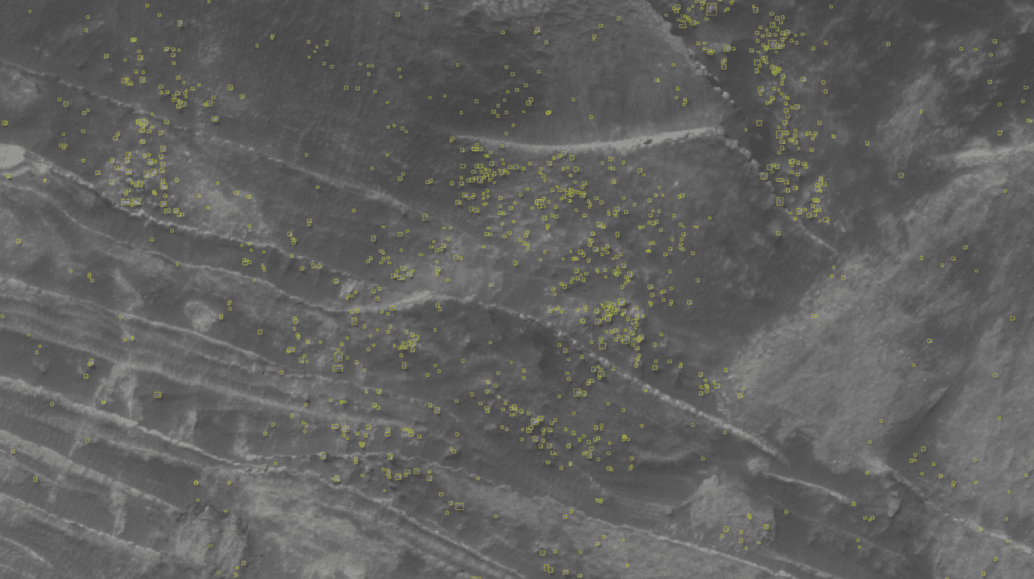
fig. 1 Multiple detections in an area with high mass wasting activity. Even the smallest instances are identified correctly.
Acknowledgments: All data for this investigation can be obtained at the HiRISE website (http://hirise.lpl.arizona.edu/) or the Planetary Data System (http://pds.nasa.gov).
References:
[1] Russell P., Thomas, N. Byrne, S. Herkenhoff, K.Fishbaugh, K. Bridges, N. Okubo, C. Milazzo, M. Daubar, I. Hansen. Seasonally active frost-dust avalanches on a north polar scarp of Mars captured by HiRISE, Geophys. Res. Lett. 35, L23204 (2008).
[2] L. Fanara, K. Gwinner, E. Hauber, J. Oberst. Present-day erosion rate of north polar scarps on Mars due to active mass wasting, Icarus, Volume 342, (2020),113434, ISSN 0019-1035.
[3] Shu Su, Lida Fanara, Haifeng Xiao , Ernst Hauber , and Jürgen Oberst. Detection of Detached Ice-fragments at Martian Polar Scarps Using a Convolutional Neural Network; ieee journal, vol. 16, 2023.
[4] Ronneberger, O., Fischer, P., & Brox, T. (2015). U-NET: Convolutional Networks for Biomedical Image Segmentation. arXiv (Cornell University). https://doi.org/10.48550/arxiv.1505.04597
[5] Sefi Bell-Kligler, Assaf Shocher, Michal Irani. Blind Super-Resolution Kernel Estimation using an Internal-GAN. arXiv:1909.06581
[6] Linlin Zhu, Xun Geng, Zheng Li and Chun Liu. Improving YOLO v5 with Attention Mechanism for Detecting Boulders from Planetary Images. Remote Sens. , 13(18), 3776 (2021).
How to cite: Martynchuk, O., Lida, F., Oberst, J., and Hussman, H.: Computer vision model for monitoring mas wasting activity in the Martian North Polar region, Europlanet Science Congress 2024, Berlin, Germany, 8–13 Sep 2024, EPSC2024-793, https://doi.org/10.5194/epsc2024-793, 2024.
Introduction
Remotely sensed hyperspectral data provide essential information on the composition of rocks
on planetary surfaces. On Mars, these data types are provided by the CRISM instrument
(Compact Reconnaissance Imaging Spectrometer for Mars) [1], a hyperspectral camera that
operated onboard the MRO (Mars Reconnaissance Orbiter) probe that collected more than 10
Tb of data over more than 14 years of operation. CRISM covers a spectral range going from
362 to 3920 nm, with a spectral resolution of 6.55 nm/channel and a spatial resolution of 18.4
m/px, from 300 km altitude.
The most advanced CRISM data products are the MTRDRs (Map-Projected Target Reduced
Data Records) [2]. These data are re-projected onto the Martian surface and are cleaned from
the so-called ”bad bands”, noisy stripes. The two main CRISM MTRDR subproducts are the
hyperspectral datacube and the spectral parameter datacube. The first contains the detected
reflectance spectra, while the second is composed of 60 different spectral parameters, as defined
in [3], usually to produce RGB maps emphasizing specific minerals within the scene.
The analysis of such products is often made by selecting Regions of Interest (ROI) from which
to extract the spectra. Recently, other more global and general methods are beginning to be
used, such those that involves the application of machine learning algorithms to analyze and/or
map the planetary surface spectra (i.e., [4]), in order to obtain more general and exhaustive
results.
Regarding the model architecture, undercomplete autoencoders represent a fundamental concept
in the domain of unsupervised learning using neural networks. At its core, an autoencoder
is a type of artificial neural network trained to reconstruct its input data at the output layer.
It consists of two main components: an encoder and a decoder. The encoder compresses the
input data into a lower-dimensional representation, while the decoder attempts to reconstruct
the original input from this compressed representation. An undercomplete autoencoder is characterized
by having a bottleneck in the network architecture, where the dimensionality of each
layer, from the first one to the encoded representation layer is lower than the previous layer
dimension. This architecture force the model to capture the most relevant information stored in
the input data, thus facilitating effective feature extraction. The train process of a undercomplete
autoencoder is no different than the training of a classical Fast Forward Neural Network,
so involving the minimization of a reconstruction loss function evaluated between the input
data and the reconstructed output.
For this work, we analyzed as a case study the CRISM named FRT00003E12
in Nili Fossae. The choice of this specific scene was motivated by the morphological and spectral
richness that it offers and by the mole of literature [5,6,7] available for comparison.
Methods
This work explores the potentials of Undercomplete Autoencoders to perform:
- The dimensionality reduction of a CRISM MTRDR product;
- the clustering of similar spectra regions and subsequent region spectra analysis;
- the generation of specific nonlinear combination of spectral parameters to enhance specific
mineralogies
In detail, we trained the networks using the spectral parameters datacube after eliminating
the pure reflectance parameters and the immediately reflectance-relatable parameters, those
being R770, RBR, RPEAK1, R440, IRR1, R1330, IRR2 , IRR3,
R530, R600, R1080, R1506, R2529 and R3920 [3]. We obtained a total number of 46 spectral
parameter for each pixel image.Then, we checked the pixel values for each spectral parameter, setting to zero each value below
zero. This was done because less than zero valued pixels do not have a physical meaning inside
the spectral parameter image. Finally, each feature were normalized with the following: xnorm = (x-xmean)/σ.
The subsequent step consisted of model selection by hyperparameter optimization. To achieve
this goal, we trained 60 random different models with various, random sampled hyperparameters
sets on a subset of the original datacube (20%) for 50 epochs.
The best model was then chosen by selecting the trial that, in 50 epochs, gave us the lowest
loss function value, where the chosen loss function was the Huber Loss, chosen as encompass
both the properties of the L1 and MSE losses ensuring so a better overall performance.
The optimizer we used for both the random search and the training process is Adam, and
the batchsize for both the final training and the hyperparameter optimization was set to the
entire image/subset. Then we trained the optimal model for 100 epochs and we extracted the
latent space for each pixel. After this we scaled the resulting pixel values setting to zero all the
pixels below the median value (constraining so between the 50th and 100th percentiles) and we
divided each pixels in different classes. Each class derives from the combination of latent space
neurons in that pixel. For example, the classes 00000 and 11111 represents all the pixels that
does not activate any latent space neuron and all that activates all the latent space neurons,
respectively (see figure 3 top left and bottom right). Finally, from each class, we extracted the
mean spectra and its standard deviation.
Table 1 and figure 1 reports the final model resulting from the random search hyperparameters
optimization process. Also, Figures 2 and 3 shows its application to the reflectance-deficient CRISM spectral parameter datacube. Figures 2 and 3 highlight that each pixel in the CRISM
datacube activates different neurons (Fig 2) and neuron combinations (Fig 3) in the latent space.
Figure 4 reports the superimposition of the different unique neuron combinations reported in
figure 3. In figure 4 b, each color represent a class of activated neurons and permits a more
direct comparison between the model’s extracted information and the morphological/albedo
features of the CRISM scenario (a). Figure 5 reports the mean spectra extracted for each
neuron combination that could be used for further investigations or for the comparison with
laboratory investigations.
Overall, we highlighted that undercomplete autoencoders could be a possible reliable instrument
for the analyses of hyperspectral datacube, from simple spectra extraction by clustering to the
generation of synthetic spectral parameters.
table 1
| L. Rate | Enc. N. | Dec. N. | W. Decay | Enc. Dim. | Act.func. |
| 0.05 | 25,15 | 45 | 0.0001 | 4 | SiLU |
figure 1
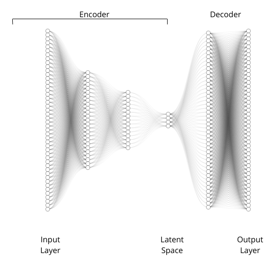
figure 2
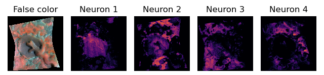
figure 3
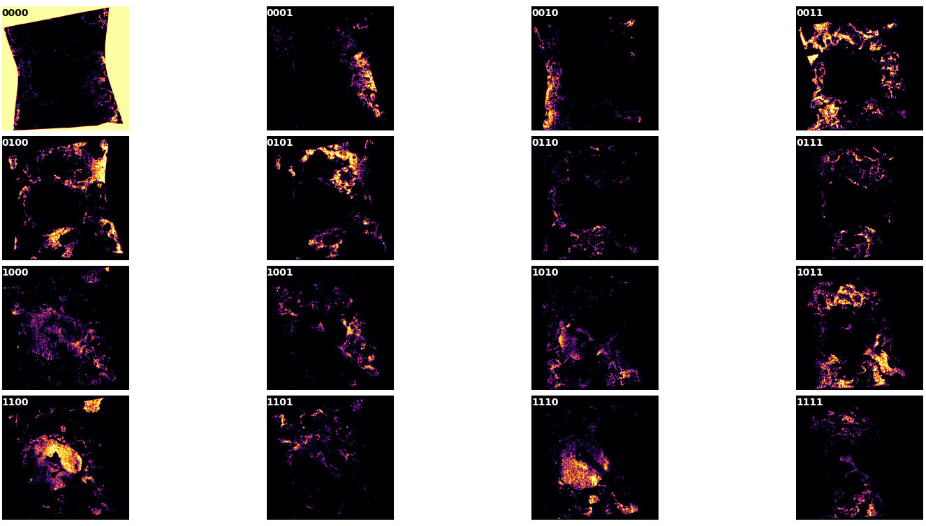
figure 4
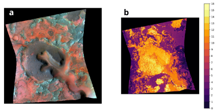
figure 5
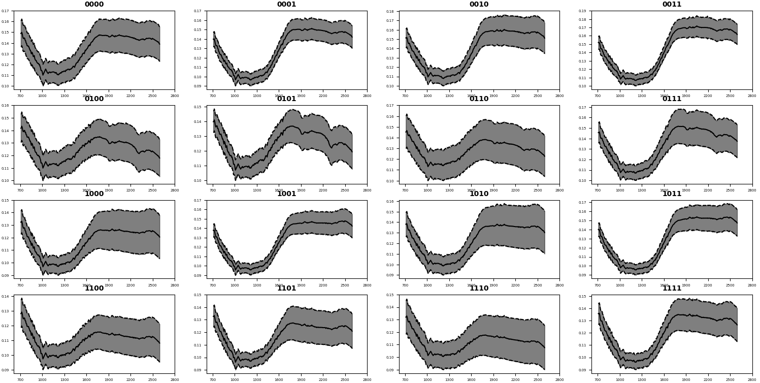
[1] Murchie2007,E05S03
[2]Seelos2016,LPSCXXXXVII
[3]Viviano-Beck2014,119(6):1403-1431
[4]Baschetti2024,XIXCongressoNazionalediScienzePlanetarie
[5]Mustard2009,doi:10.1029/2009JE003349.
[6]Elhmann2008,Science,322,1228-1832
[7]Mustard2008,https://doi.org/10.1038/nature07097
https://doi.org/10.1038/nature07097
How to cite: Baroni, M., Pisello, A., Petrelli, M., and Perugini, D.: Automatic CRISM mapping and spectral parameter generation using undercomplete autoencoders, Europlanet Science Congress 2024, Berlin, Germany, 8–13 Sep 2024, EPSC2024-1133, https://doi.org/10.5194/epsc2024-1133, 2024.
Introduction: Mars possesses a strong remanent crustal field, indicative of an ancient magnetic dynamo which is now inactive [1]. Such a dynamo is associated with the internal composition and thermal evolution of early Mars. Thus, crustal magnetic fields record invaluable insights into the early stages of this planet, and our objective is to map out their distribution. We address the problem of modelling the crustal magnetic field using magnetometer measurements from two orbiters, MGS and MAVEN. A substantial amount of additional low-altitude data has been collected by MAVEN since the most recent and highest resolution global model was published ([3], referred to as L19 in the following), thereby necessitating a new model to be computed. Two approaches were formally used for this: Spherical Harmonics (SH, e.g., [2]) and Equivalent Source Dipoles (ESD, e.g., [3]). We propose to solve this regression problem with Physics-Informed Neural Networks (PINN). Intuitively, this method is comparable to that of a Spherical Harmonic model, with basis functions that are not a priori defined but uniquely suited to the regression task at hand. We show that this alternative has multiple advantages such as computational efficiency and robustness to sparse distributions.
Data: MGS (1997 – 2006) and MAVEN (since 2014) provided time series of the magnetic field measured at orbital altitude. While MGS was in a nearly constant altitude orbit most of the time, MAVEN has a much more eccentric orbit. This offers the advantage of probing the entire magnetic field environment but also lacks repeated orbits. Because low altitude data contains small-wavelength information, a model including the latest lower-altitude data from MAVEN should theoretically enhance the resolution of small-scale features.
Modelling: Physics-informed neural networks (PINN) embed the knowledge of any physical laws that govern a given dataset in the learning process of a neural network. For our crustal field model, the network takes three parameters as input, point coordinates, and outputs a scalar potential. The free parameters, analogous to dipole components for the ESD approach, or to Gauss coefficients for SH, are the weights and biases of each neuron in the network that connect inputs and outputs through an array of interconnected layers. The predicted B-field is computed from this scalar potential with automatic differentiation before updating the free parameters with back-propagation.
The datasets from MGS and MAVEN orbiters differ too greatly to be treated equivalently. The former represents densely collected data at nearly constant altitude, whereas the latter is sparse, but distributed across a larger altitude range including lower altitudes. We therefore adapt our modelling strategy to these characteristics. A network is trained for each altitude band independently and the resulting preliminary models are used to remove outliers from the data.
A problem with inputs in spherical coordinates is that of model continuity at poles and along the longitude boundary. The model does not inherently know that longitude 180° is equal to longitude -180°. To overcome this issue without loss of accuracy, one could either reparametrize the data into cartesian coordinates or decompose the periodic component into a weighted summation of the basis functions of Fourier series. Given that neural networks are approximators of nonlinear continuous functions, the sole first two basis functions suffice [4].
Discussion: There are four main reasons why we believe that PINN can perform better in achieving this regression. First of all, for a given regression task, neural networks are more memory-efficient than traditional least-squares methods like SH or ESD which require inverting large matrices. This circumvents the former necessity of down sampling the extensive datasets, thereby losing information. Second, modern neural network algorithms come with an arsenal of tools enabling to find the optimum between under and over-fitting of the data, such as validation and early stopping, without explicit regularizations. Thirdly, PINN is a very powerful method to discriminate the data according to any physical assumptions we may have. For instance, imposing ∇×B = 0 as a soft constraint will reward field data originating from the crust that is conservative and punish field data that results from induced currents in the ionosphere. Lastly, this method combines the benefits of both SH and ESD. The ESD method was proposed as an alternative to SH for its robustness to data sparsity [5]. However, ESD has the disadvantage of being inherently ill-conditioned – the Gram matrix becomes less invertible as spatial resolution improves [6]. PINN is impacted by neither of these issues.
First Results and Outlook: The first results from this novel approach are promising. Fig. 2 shows the observed magnetic field components along a quiet orbit of MAVEN compared with predictions by the L19 model [3], and by our early model (outliers not yet filtered). We can observe that it is locally outperforming L19. Moreover, a 200km map of the predicted scalar field using our PINN model and the unfiltered MAVEN data shows an unprecedented resolution (Fig. 3). Even though we did not use any regularization, nor down sampled the data, we do not observe linear features following individuals tracks, a typical feature for unregularized models. This observed smoothness indicates that the data is not overfitted.
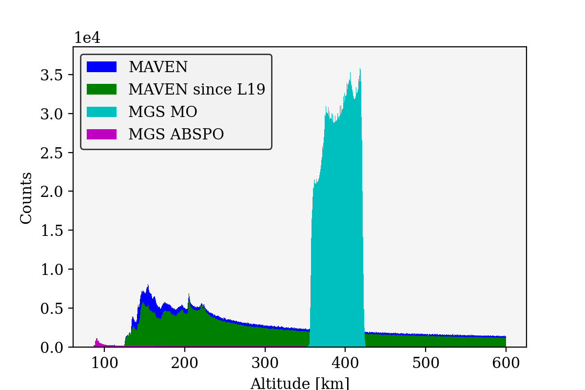
Fig.1: Histogram of the altitude distribution of the nighttime data from MGS and MAVEN orbiters. An important part of the low-altitude data has been produced after the last global model L19 [3].
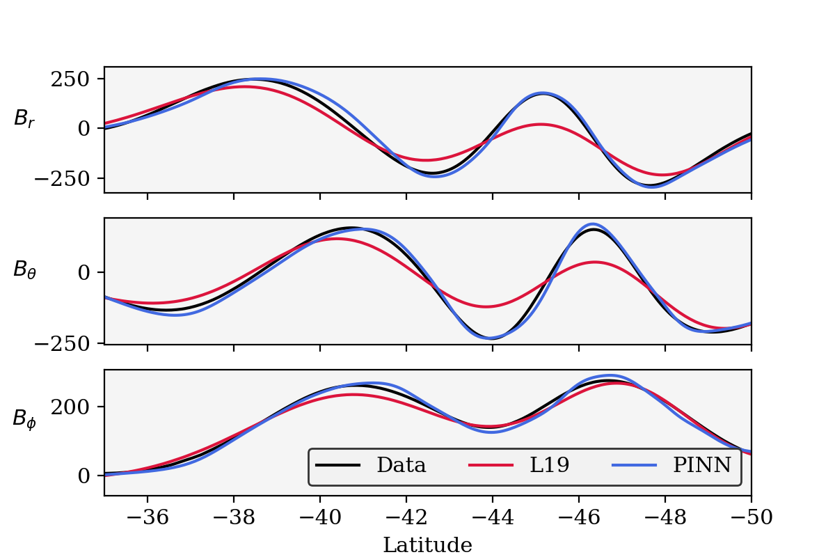
Fig.2: Observed and predicted magnetic field along an orbit of MAVEN (23-04-2023). PINN has more predictive value than L19 [3] for quiet orbits.
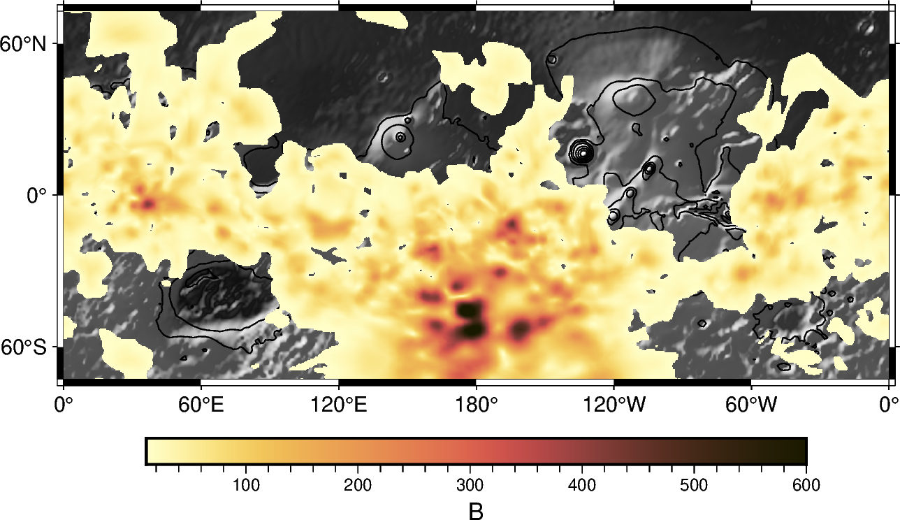
Fig.3: Map of the predicted scalar field at 200km using our PINN model and the unfiltered MAVEN data only.
Acknowledgments: This work is supported by SNF Ambizione (PZ00P2_209123).
References: [1] Acuna et al. (1999) Science, xx. [2] Morschhauser, A., et al. (2014) Journal of Geophysical Research: Planets 119.6, 1162-1188. [3] Langlais, B., et al. (2019) Journal of Geophysical Research: Planets 124.6, 1542-1569. [4] Lu, L., et al. (2021) SIAM Journal on Scientific Computing, 43(6), B1105-B1132. [5] Mayhew, M. A., and Estes, R. H. (1982) NAS 1.26: 169604. [6] Blakely, R. J. (1996) Cambridge University Press.
How to cite: Delcourt, T. and Mittelholz, A.: A New Model of the Litospheric Magnetic Field of Mars using a Physic-Informed Neural Network, Europlanet Science Congress 2024, Berlin, Germany, 8–13 Sep 2024, EPSC2024-1175, https://doi.org/10.5194/epsc2024-1175, 2024.
- Introduction
Large area, high-resolution, three-dimensional (3D) mapping of a planetary surface is not only essential for performing key science investigations on the formation and evolution of the surface, but is also critical for planning and supporting existing and future surface robotic missions as well as planning human exploration. Over the past 20 years, 3D mapping of the Moon surface has only been performed for larger areas with low-resolution data, or for very small areas with higher-resolution data.
Large area lower-resolution 3D mapping work usually refers to the global lunar digital terrain models (DTMs) created from the NASA Lunar Orbiter Laser Altimeter (LOLA) and LOLA altitudes blended with the Japanese SELenological and Engineering Explorer (SELENE) DTMs from the Kaguya Team at a grid-spacing at 118 m/pixel and 60 m/pixel, respectively, or using the Chang’E-2 3D image products at 7mpp or 3D map products at 20mpp. On the other hand, smaller area higher-resolution 3D mapping work usually employs the LROC Narrow Angle Camera (NAC) images at 0.5-1.5 m/pixel producing DTMs at about 5m/pixel using photogrammetry or DTMs at 0.5-1.5 m/pixel using photoclinometry.
The limitations of having to trade-off between “large area” and “high-resolution”, for lunar 3D mapping is a consequence of three different aspects. Firstly, lower-resolution data such as LROC WAC and Chang’E-2 (CE-2) generally have better stereo coverage, whereas the main high-resolution data to date (LROC NAC) only has limited stereo coverage (≤1% of the lunar surface). Secondly, the photogrammetry and photoclinometry processes are complex and subject to different errors (or artefacts) at each of their different processing stages, which require specialist expertise to deal with these complexities in order to produce high-quality DTM products, especially over large areas. Thirdly, the expensive computational cost from existing photogrammetry and photoclinometry pipelines makes it extremely difficult to achieve large area high-resolution coverage in any realistic time-scale.
To address these limitations, a single input image-based rapid surface modelling system has been developed, called MADNet 2.0 (Multi-scale generative Adversarial U-net with Dense convolutional and up-projection blocks) [1] to create high-resolution DTM products for the NASA MoonTrek system previously for the von Karman crater [2]. Here we apply MADNet to 7 of the 13 ARTEMIS landing sites near the lunar south pole which have very different illumination conditions.
- Methods
27 higher resolution LOLA DTMs of 5 mpp (usually they are 118 mpp) were processed by the NASA GSFC LOLA team [1] and are shown in Figure 1.
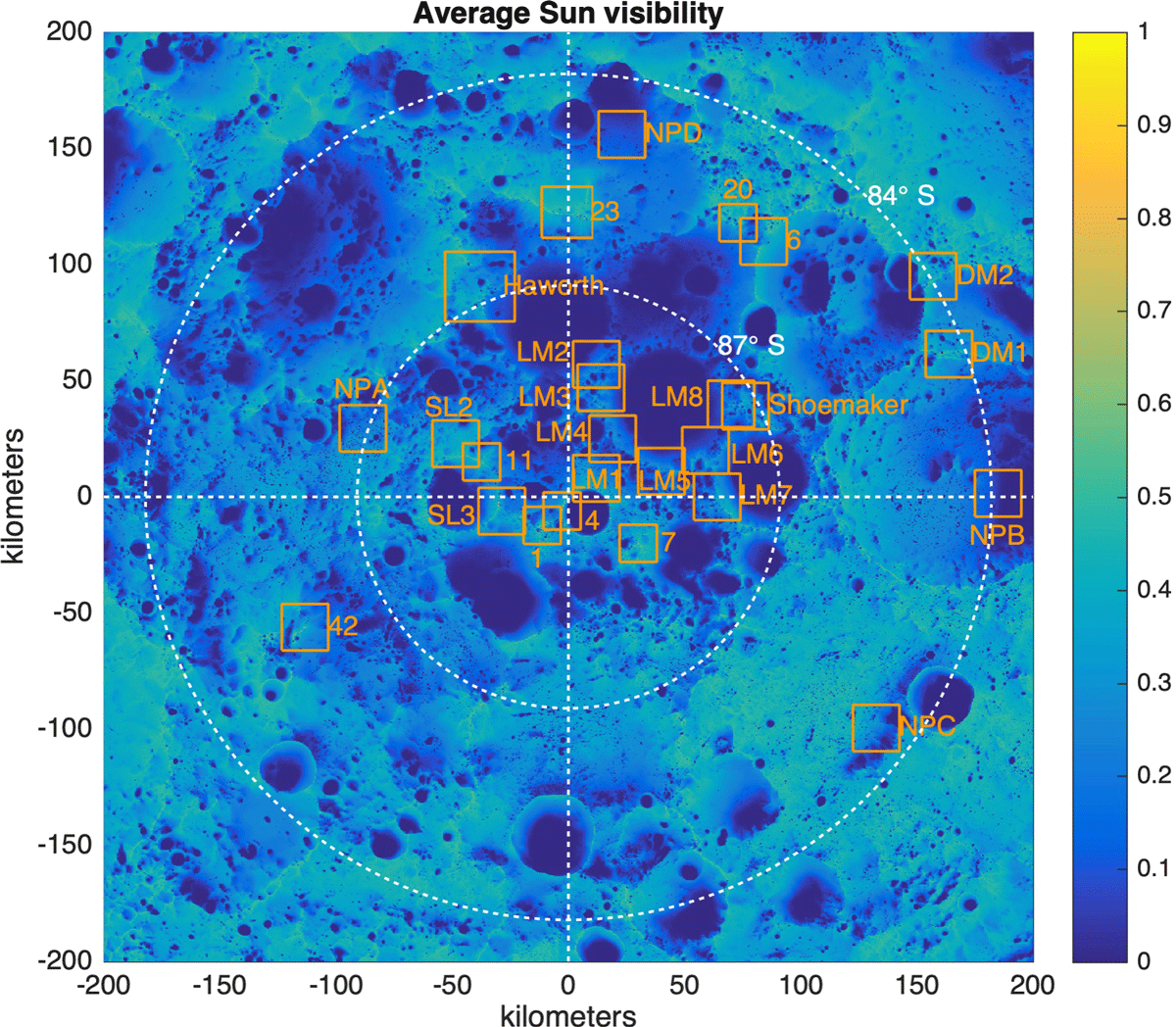
Figure 1. Display of 5 m/pixel LOLA DTMs created by the NASA GSFC LOLA team against a background generated from the LOLA 118 m/pixel global DTM. Our focus here is on the generation of 1m MADNet DTMs covering areas marked as Haworth, 23, 20, 6, DM1, DM2 and 7. Figure taken from https://pgda.gsfc.nasa.gov/products/78
A description of the overall MADNet processing chain can be found in [1] and Figure 2.
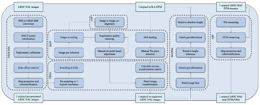
Figure 2. Flowchart of the MADNet 2.0 processing chain for DTM retrieval of single LROC-NAC images
A key requirement is the training of the network using pre-existing photogrammetrically derived DTMs consisting of 22,084 ORI-DTM training pairs (512*512 pixels at 5 m/pixel) which were formed using 392 pairs of single-strip downsampled 5 m/pixel LROC NAC PDS ORIs and 5 m/pixel stereo DTMs with horizontal and vertical flipping. The LROC NAC DTM processing includes 1) initial input selection (247 single-strip EDR data downloaded) and screening (103 out of 247 selected) for non-overlapping, quality and shadow control; 2) USGS-ISIS based pre-processing for format conversion (from PDS to ISIS CUBE), geometric calibration, artefact/noise removal and SPICE kernel initialisation, USGS-ISIS map-projection and orthorectification (cam2map) w.r.t. LOLA; 3) LROC NAC image co-alignment using the NASA Ames Stereo Pipeline (ASP)’s image_align method; 4) Manual tie-point based LROC NAC image co-registration with 5 m/pixel LOLA DTM; 5) MADNet based image-to-DTM inference that follows the standard MADNet 2.0 processing chain that is described in [1,2]; 6) ASP based tile and DTM mosaicing, as well as LROC NAC image orthorectification.
- Results
Seven 20 x 20 sq.km areas were processed but where there were significant gaps due to permanent shadows, these had to be filled in using the 5 mpp LOLA DTMs. Neither the NASA Shadowcam instrument [4] nor the Chandraya’an-2 OHRC [5] have sufficient coverage at present. Only 2 of the 7 sites show coverage > 50% as shown in Table 1.
Table 1. Summary of the higher-resolution LROC NAC DTM pixel coverage for the LOLA filled LROC NAC DTM mosaics of each site.
|
Site name |
LROC NAC DTM pixel coverage % |
|
Amundsen Rim |
54.33% |
|
Haworth |
20.12% |
|
Leibnitz Beta Plateau |
36.43% |
|
Malapert Massif |
40.77% |
|
Nobile Rim 1 |
40.35% |
|
Nobile Rim 2 |
49.47% |
|
Peak Near Shackleton |
51.78% |
Several example DTMs are shown here at 1mpp in Figures 3-6 as follows:
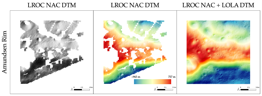
Figure 3. 1 m/pixel LROC NAC DTM products for Amundsen Rim
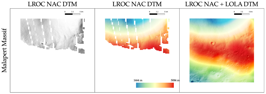
Figure 4. 1 m/pixel LROC NAC DTM products for Malapert Massif
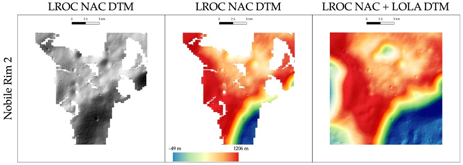
Figure 5. 1 m/pixel LROC NAC DTM products for Nobile Rim 1.
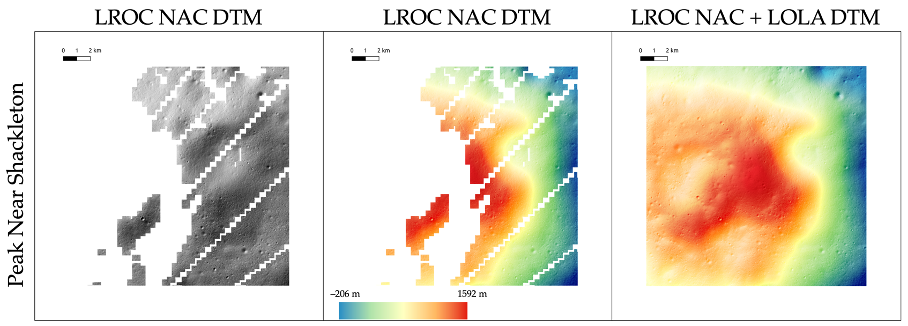
Figure 6. 1 m/pixel LROC NAC DTM products for Peak Near Shackleton
- Discussion and Conclusions
One metre DTMs were created from single image LROC-NAC images using the MADNet 2.0 DTM retrieval system which covered up to 54% of the 20 x 20km area. Significantly more detail is shown in the 1mpp DTMs compared with the LOLA 5 mpp DTMs. In order to fill these gaps in future, there need to be sufficient Shadowcam and/or Chandraya’an-2 OHRC shadow images and corresponding stereo DTMs at lower resolution for updating the training of the MADNet prediction model. All of these products will be released through the ESA Guest Storage Facility at https://www.cosmos.esa.int/web/psa/ucl-mssl_meta-gsf as well as through the NASA Moontrek system.
Cited references
[1] Tao, Y.; Muller, J.-P et al. Remote Sens. 2021, 13, 4220.
[2] Tao, Y.; Muller, J.-P. et al. Remote Sens. 2023, 15, 2643.
[3] Barker, M.K., et al. (2021),. https://doi:10.1016/j.pss.2020.105119.
[4] Robinson et al., 2023, J. Astron. and Space Science.
[5] Prateek Tripathi & Rahul Dev Garg doi: 10.5194/epsc2021-83
How to cite: Muller, J.-P., Tao, Y., and Walter, S. H. G.: Digital Terrain Models of the NASA ARTEMIS sites from single LROC-NAC images using the UCL MADNet retrieval system., Europlanet Science Congress 2024, Berlin, Germany, 8–13 Sep 2024, EPSC2024-1170, https://doi.org/10.5194/epsc2024-1170, 2024.
Introduction
The final phase of planet formation involves the growth of planetesimals through pairwise collisions of bodies up to the size of planets in protoplanetary discs. Studying this final phase, numerical methods are used to investigate collisions and thus the formation of planets.
N-body simulations can be used to model the dynamical evolution of circumstellar disks, including planet formation [1]. Gravitational N-body models fail as soon as the bodies touch, hence models for treating collisions must be added. A general and flexible approach by Burger et al. [1] resolves collisions by running dedicated Smoothed Particle Hydrodynamics (SPH) simulations for each collision.
Accurate methods, such as SPH, are computationally intensive and time-consuming. To achieve faster, yet accurate results, there are approaches using different machine learning (ML) methods on SPH datasets. Winter et al. [2] use comprehensive SPH datasets including rotating bodies. They utilize ML models (instead of SPH) to predict collision outcomes.
Independent from planet formation, recently, neural networks have been successfully applied to the approximation of numerical N-body and particle-based fluid dynamics simulations. They utilize graph neural networks (GNN) to handle particle representations, e.g. point clouds like SPH representations. In addition, Martinkus et al. [3] introduce GNNs with a hierarchical architecture to handle large numbers of particles. Current approaches use equivariant neural networks that induce geometric properties. Inductive biases such as E(3)-equivariance might lead to faster training convergence and improved generalization.
Aim of this work
Classical simulation methods for planetary collisions are particle-based. However, previous machine learning approaches for planetary collisions do not use particle-based models and mainly consider macroscopic properties of collisions. Such methods allow physical interpretation only to a certain degree. A more general approach requires modelling small-scale physical interactions as in the particle based classical methods.
Therefore, we develop a model for particle-based simulations that is suitable for complex simulations such as planetary collisions. We propose combining equivariant graph neural networks with a hierarchical tree architecture. This enables learning SPH particle representations directly by processing scalar and vectorial physical quantities in a scalable manner. Since calculating all particle interactions scales quadratically with the number of particles (O(n2)), dense connectivity becomes costly in case of many particles. Therefore, the hierarchical tree architecture is used similar to classical numerical particle simulation techniques to approximate the interactions of long-range forces. The utilized hierarchical tree reduces the computational complexity to O(n) in the tree and O(n log(n)) for building the tree while retaining long-range interactions like gravity.
So, our ML model replaces SPH simulations for planetary collisions within classical N-body frameworks.
Methods
Dataset:
We use a small SPH dataset derived from the dataset by Winter et al. [2] which is based on statistics derived from Burger et al. [1]. The dataset includes pure hydrodynamic SPH simulations with self-gravity of pairwise planetary collisions with varying collision angles and velocities. Bodies consist of iron cores and basalt mantles of different sizes.
Model:
We take SPH representations as a point cloud and build a graph by representing the interactions with the neighbour particles for every particle by edges. Our model is based on a scalable E(3)-equivariant GNN (SEGNN) [4]. To create a model that is scalable to high numbers of particles, we add a hierarchical graph architecture inspired by the fast multipole method [3] and call it hierarchical SEGNN (HSEGNN).
SEGNN takes graphs with fixed numbers of neighbours using a KNN algorithm to find the connected neighbours and applies equivariant convolutions on that graph. The connections in the hierarchical graph are derived by the tree algorithm.
We use an autoregressive model which iteratively predicts the state after a fixed time step from an initial state. These ML time steps can be much larger than the classical simulation time steps. Our models are trained with common, gradient-based optimization methods.
Results
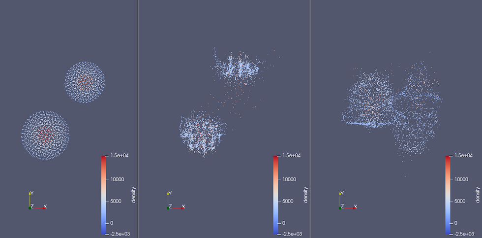
a) Time step 3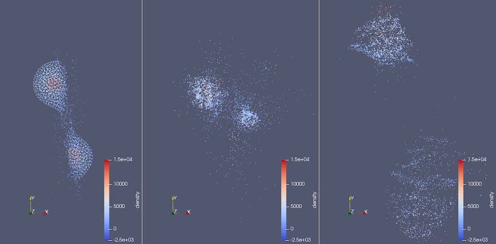
b) Time step 6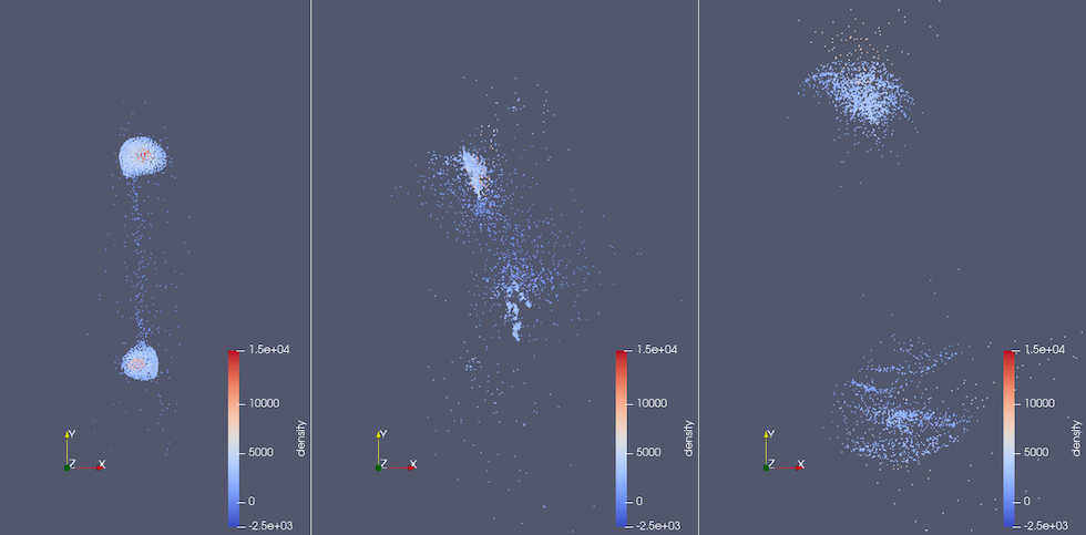
c) Time step 10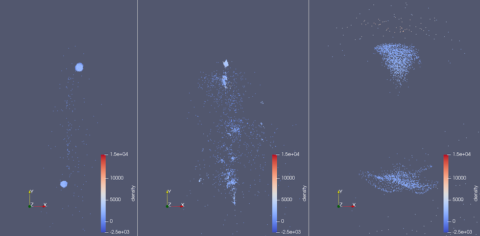
d) Time step 25
Figure 1.: Collision time steps' ground truth (left), prediction of the HSEGNN (middle) and prediction of the SEGNN (right) before and during collision. Each SPH particle is represented as a point. The ML time steps 3,6,10 and 25 are shown from top to bottom. One ML time step corresponds to 10 minutes in simulation time. The density is color-coded.
Figure 1 shows snapshots of one of our test simulations. Colour scales indicate rough boundaries between iron cores and basalt mantles. Both HSEGNN and SEGNN capture the overall evolution of large fragments to a certain extent while suffering from unrealistic predictions on smaller scales. However, HSEGNN retains individual fragments better than SEGNN which suffers from unrealistic diffusion artefacts.
We conclude that although both methods require improvements to produce physically plausible results, HSEGNN shows improved capabilities for mapping material forces within fragments.
Runtime:
The ML models achieve speed advantages by a factor of 100 compared to the SPH simulations. However, the duration to build the hierarchical graph is within the runtime range of the SPH simulations. The implementation of our tree algorithm has capabilities for speed improvements to make the overall model faster than the SPH simulations. Shorter runtimes are the main advantage of ML methods over classic simulation methods in this application.
Acknowledgements
The authors acknowledge support by the state of Baden-Württemberg through bwHPC and the German Research Foundation (DFG) through grant no INST 37/935-1 FUGG.
References
[1] Burger, C., Á. Bazsó, and C. M. Schäfer (2020). “Realistic collisional water transport during terrestrial planet formation”. In: Astronomy & Astrophysics 634, A76.
[2] Winter, Philip M. et al. (2023). “Residual neural networks for the prediction of planetary collision outcomes”. In: Monthly Notices of the Royal Astronomical Society 520.1, pp. 1224–1242.
[3] Martinkus, Karolis, Aurelien Lucchi, and Nathanaël Perraudin (2021). “Scalable Graph Networks for Particle Simulations”. In: Proceedings of the AAAI Conference on Artificial Intelligence 35.10, pp. 8912–8920.
[4] Brandstetter, Johannes et al. (2022). “Geometric and Physical Quantities improve E(3) Equivariant Message Passing”. In: International Conference on Learning Representations.
How to cite: Hohaus, J., Winter, P. M., and Schäfer, C.: Scalable E(3) Equivariant Graph Neural Networks for Particle Simulations, Europlanet Science Congress 2024, Berlin, Germany, 8–13 Sep 2024, EPSC2024-1087, https://doi.org/10.5194/epsc2024-1087, 2024.
Introduction
Hera is ESA’s first planetary defense mission designed to characterize the binary near-Earth asteroid (65803) Didymos [1]. Its secondary component, Dimorphos, was the target of the large-scale controlled collision with the NASA/DART spacecraft in September 2022 [2]. Thus, the Hera mission will provide an unprecedented opportunity to study the aftermath of the first ever artificial asteroid impact. This will be done with the help of several instruments, including the hyperspectral camera HyperScout-H (HS-H).
The goal of this work is to prepare the algorithms required to analyze the future data coming from HS-H. We aim to determine the surface morphology and its composition, including the characterization of space-weathering effects and the search for exogenous material. We are implementing machine learning (ML) approaches to classify the different surface patches using the asteroid spectral (taxonomic) classification. This abstract presents preliminary results on the spectral classification considering the nature of the data that will be acquired by HS-H. To perform several simulations, we use imaging data sourced from the JAXA/Hayabusa spacecraft equipped with the Asteroid Multi-band Imaging Camera (AMICA) [3, 4, 5, 6]. The reason for this choice is the expected similarity between the asteroid studied by JAXA/Hayabusa – (25143) Itokawa, and the target of ESA/Hera – (65803) Didymos.
Methods
The reflectance spectrum of an asteroid, R(λ), is usually observed in the visible and near-infrared domains between 0.35 and 2.50 μm and can be classified into several types. One of the most used taxonomic classifications was defined in [7] using Principal Component Analysis (PCA) over a set of 371 spectra of asteroids. This uses letters to characterize the composition of the asteroids and it helps to perform various statistical studies over large populations of these celestial objects. Here, we develop a predictive model that accurately classifies the asteroid surface patches based on the reflectance spectrum observed by HS-H. The spectral window observed by HS-H spans the interval 0.657 – 0.949 μm. Each 5 x 5 macropixel on the mosaic filter on the HS-H detector records the signal within 25 narrow bands (25 pixels), each one with a different effective wavelength. Considering the spectral response of each band, it is challenging to accurately retrieve the true reflectance spectra due to the filter transmittances and spatial distribution.
To compare the HS-H spectrum with other spectra we need to consider the transmission functions of HS-H. Thus, we simulate an asteroid spectrum observed with HS-H. The converted reflectance is obtained by integrating over the transmission function domain in each band, i.e. ∫R(λ)τ(λ)dλ, where τ(λ) is the transmission function value at λ of one of the HS-H bands. An example is provided in Fig. 1 (a). Then, for each input data we get the equivalent HS-H observed spectrum containing 25 reflectance values computed for each one of the HS-H bands, and the spectral class that can be represented with a one-hot encoded vector. Thus, the learning problem is based on finding the best multi-class classifier. This is typically achieved by training a classifier (i.e. neural network) to predict the probability distribution over the classes by minimizing the cross-entropy loss, which is a measure of the dissimilarity between the predicted probability distribution and the true distribution.
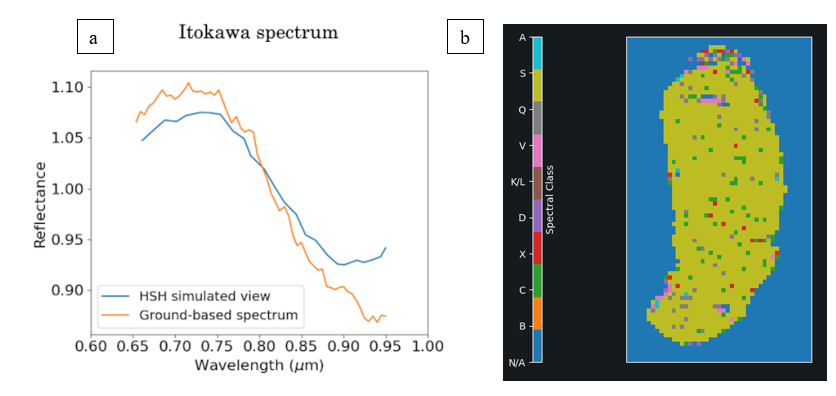
Fig. 1 (a) Comparison between the HS-H simulated spectrum of Itokawa and the spectrum obtained from ground-based observations (b) Spectral classification map retrieved by applying the CNN on the simulated representation of Itokawa.
Data analysis and results
We utilize the dataset described in [8] containing up to 3000 spectral samples from various asteroids. We select 11 classes that are the most relevant for our study case. We split the dataset such that 60% of the data is used for training, 20% for validation, and 20% for testing. We perform a stratified split, meaning that there are enough samples of each taxonomic class in each set. Each spectrum is interpolated by a spline curve to obtain a fit for the reflectance spectrum and to apply the transmission functions of HS-H. The data is augmented as needed by small shifts or rotations, or by adding noise like that produced by the HS-H instrument.
We implement traditional ML algorithms such as k-Nearest Neighbors, Decision Tree and Random Forest which we optimize via grid search. Also, we try different dense (DNN) and convolutional (CNN) neural network architectures aiming to get the best accuracy by width and depth scaling. A comprehensive analysis of these methods is done to choose the best classifier and obtain accurate classification maps, as the one shown in Fig. 1 (b), where we apply the CNN on the simulated data for asteroid Itokawa to determine the spectral class in each macropixel and to check the homogeneity.
Our preliminary results on the spectral classification applied on simulated data of Itokawa are promising. A quick comparison with the images from [6] shows that we were able to identify various spectral patterns across Itokawa’s surface. We plan to simulate other test case scenarios by superimposing various patterns into the original data.
References
[1] P. Michel et al. The ESA Hera Mission: Detailed Characterization of the DART Impact Outcome and of the Binary Asteroid (65803) Didymos. , 3(7):160, July 2022.
[2] Andrew S. Rivkin et al.. The double asteroid redirection test (dart): Planetary defense investigations and requirements. The Planetary Science Journal, 2(5):173, aug 2021.
[3] J Saito et al. Detailed images of asteroid 25143 itokawa from hayabusa. Science (New York, N.Y.), 312:1341–4, 07 2006.
[4] Masateru Ishiguro et al. Global mapping of the degree of space weathering on asteroid 25143 Itokawa by Hayabusa/Amica observations. Meteoritics & Planetary Science, 42(10):1791–1800, 2007.
[5] Eri Tatsumi, Seiji Sugita. Cratering efficiency on coarse-grain targets: Implications for the dynamical evolution of asteroid 25143 Itokawa, Icarus, Volume 300, 2018, Pages 227-248.
[6] Sumire C. Koga et al. Spectral decomposition of asteroid Itokawa based on principal component analysis. Icarus, 299:386–395, 2018.
[7] Francesca E. DeMeo et al. An extension of the Bus asteroid taxonomy into the near-infrared. Icarus, 202(1):160–180, 2009.
[8] M. Mahlke et al. Asteroid taxonomy from cluster analysis of spectrometry and albedo. AA, 665:A26, September 2022.
How to cite: Prodan, G. P., Popescu, M., de León, J., Tatsumi, E., Grieger, B., Licandro, J., Kohout, T., and Küppers, M.: Machine Learning for Future Hyperspectral Data Analysis with the Hyperscout-H instrument on the ESA’s Hera Mission, Europlanet Science Congress 2024, Berlin, Germany, 8–13 Sep 2024, EPSC2024-916, https://doi.org/10.5194/epsc2024-916, 2024.
Please decide on your access
Please use the buttons below to download the supplementary material or to visit the external website where the presentation is linked. Regarding the external link, please note that Copernicus Meetings cannot accept any liability for the content and the website you will visit.
Forward to presentation link
You are going to open an external link to the presentation as indicated by the authors. Copernicus Meetings cannot accept any liability for the content and the website you will visit.
We are sorry, but presentations are only available for users who registered for the conference. Thank you.
Advancements in artificial intelligence (AI) have opened new horizons for space exploration, particularly in the domain of astrometry. This research investigates the integration of AI techniques, specifically deep neural networks, with space astrometry using the Cassini-Huygens images database. The primary objective is to train a neural network for the detection and classification of astronomical sources, in particular stars, satellites and cosmic rays, in order to process them for a better understanding of our solar system, performing an analysis on the spatial and temporal variation of cosmic rays and moreover to a wider investigation on the characteristics of the Saturn system.
The methodology employed involves a multi-step process. Firstly, known stars and satellites' positions are located in the images using ARAGO (IMCCE), a software package designed for the astrometric measurement of natural satellite positions in images taken using the ISS of the Cassini spacecraft, resulting in more than 13,000 images (8bit, 1024x1024, exposure duration <= 1 s) correctly calibrated. Consequently a personalised detection system, using classical image processing techniques such as mathematical morphology, is applied to identify all the bright sources within the images, subsequently forming a labeled database for every image including source positions, bounding boxes and corresponding classes—divided in stars, satellites, cosmic rays.
The database is used to train a YOLOv5 [1] architecture, customised for small object detection, enabling the accurate identification and classification of sources within Cassini images. Due to the different characteristics of the images in the dataset, having a robust detection algorithm is challenging, considering that there is not a ground truth of the signal. It is therefore very hard to detect every source on the images. In order to minimize this issue, every image is divided in four sub-images with a small overlap between them, leading to two main benefits: firstly there is a more constant background on the sub-images allowing an easier background estimation that leads to an easier detection of sources and secondly smaller images are preferable for YOLO training, being optimised for images of size ~ 640x640.
After those targeted modification the overall precision of the network is ~ 90%.
The attained outcome is satisfactory for the moment in the context of characterizing cosmic rays’ behavior and in particularl their interaction with Saturn's magnetosphere. Preliminary findings suggest a direct relationship between cosmic rays occurrence and distance from Saturn, with a peak observed in the area outside the magnetosphere’s edge, followed by a decline in cosmic ray incidence with increasing distance from the outer edge of the magnetosphere. Significantly heightened cosmic ray levels has been noted within Saturn's closest proximity (3-8 Rs apart), potentially linked to Enceladus’ plasma emissions [2]. Indeed at Saturn, neutral atoms dominate over the plasma population in the inner magnetosphere, and local source/loss process dominate over radial transport out to 8 RS .
In conclusion, the fusion of artificial intelligence and space astrometry, as demonstrated in this study, introduces a promising paradigm for the exploration of the universe and in particular our solar system.
[1] ‘You Only Look Once: Unified, Real-Time Object Detection’: https://arxiv.org/abs/1506.02640
[2] Bagenal, F. (2011) Flow of mass and energy in the magnetospheres of Jupiter and Saturn
How to cite: Quaglia, G., Lainey, V., and Tochon, G.: Artificial intelligence at the service of space astrometry: a new way to explore the solar system, Europlanet Science Congress 2024, Berlin, Germany, 8–13 Sep 2024, EPSC2024-318, https://doi.org/10.5194/epsc2024-318, 2024.
Abstract
In recent years, the integration of artificial intelligence (AI), especially machine learning (ML), has found entrance in various fields, including industry, medicine, self-driving cars and daily life. However, the application of ML tools in space science is still in its early stages and holds the potential to complement traditional methods. This study investigates the effectiveness of machine learning algorithms, with a focus on Physics Informed Neural Networks (PINNs) to expand or support the classical methods in orbit propagation and determination.
PINNs were first introduced by Raissi et al. [1] and offer a promising avenue due to their unique ability to incorporate the governing differential equations of the system into the learning process, thereby imposing a physical constraint on the Networks predictions. This constraint enables effective training with sparse data, bypassing the need for large datasets typical for traditional Neural Network approaches. In addition, PINNs allow for the determination of unknown or poorly known parameters within the differential equation - a capability absent in conventional “Black-Box” Neural Networks.
To demonstrate the usefulness of PINNs, we first present a case study on simulated data within the framework of the AI4POD (Artificial Intelligence for Precise Orbit Determination) software tool of RSOs in the low earth orbit. A similar approach using Physics Informed Extreme Learning Machines was successfully conducted by Scorsoglio et al. [2] for simulated data. In contrast to this Single Layer architecture our approach incorporates a Deep Feed Forward Neural Network topology with a physics informed loss function. As a real case scenario, we
test the machine learning algorithm on data of the Rosetta mission [3] orbiting comet 67P/Churyumov-Gerasimenko and present preliminary results of the study.
Acknowledgements
The project Artificial Intelligence for Precise Orbit Determination (AI4POD) is funded by Deutsches Zentrum für Luft- und Raumfahrt, Bonn-Oberkassel, under grant 50LZ2308.
References
[1] M. Raissi, P. Perdikaris, G.E. Karniadakis, Physics-informed neural networks: A deep learning framework for solving forward and inverse problems involving nonlinear partial differential equations,Journal of Computational Physics, Volume 378,2019, Pages 686-707, ISSN 0021-9991, https://doi.org/10.1016/j.jcp.2018.10.045
[2] Scorsoglio, A., Ghilardi, L. & Furfaro, R. A Physic-Informed Neural Network Approach to Orbit Determination. J Astronaut Sci 70, 25 (2023). https://doi.org/10.1007/s40295-023-00392-w
[3] Andert, T., Aigner, B., Dallinger, F., Haser, B., Pätzold, M., Hahn, M., 2024. Comparative Analysis of Data Preprocessing Methods for Precise Orbit Determination, in: EGU24-19558. Presented at the EGU General Assembly 2024, Vienna, Austria. https://doi.org/10.5194/egusphere-egu24-19558.
How to cite: Dallinger, F., Aigner, B., Andert, T., and Pätzold, M.: Physics Informed Neural Networks as addition to classical Precise Orbit Determination, Europlanet Science Congress 2024, Berlin, Germany, 8–13 Sep 2024, EPSC2024-514, https://doi.org/10.5194/epsc2024-514, 2024.
Stability maps of planetary system can be carry out through numerical simulations, which require lot of computational efforts. This project propose a machine learning approach to forecast stable orbits around a planet. We generated our dataset used to train and test machine learning algorithms by runing an ensemble of 100,000 dimensionless numerical simulations of the three-body problem. In these simulations, we modeled a system with a star, a planet, and a test particle in an S-type orbit around the planet using. Rebound package and IAS15 integrator. The dataset is composed of nine features that represent the initial conditions of each numerical simulation. These features include the mass ratio of the system, planet eccentricity and true anomaly, particle orbital elements such as semi-major axis, eccentricity, inclination, argument of pericenter, longitude of node, and true anomaly. Each data point in our dataset is labeled as either stable or unstable. Everytime when the particle collided with massive bodies or was ejected from the system was consider unstable, if the particle survived throughout the entire simulation, it was classified as stable.
The overall outcome of our numerical simulations shows that 11.83% of samples in the dataset represent stable systems, while 88.17% are unstable. Among the unstable samples, 47.22% particles collided with the planet, and 40.95% were ejected from the system. This imbalance in class distribution can introduce biases and diminish the effectiveness of algorithm performance. To tackle with this issue, we evaluated the performance of our machine learning model using five different resampling techniques: random undersampling, random oversampling, SMOTE, Borderline SMOTE, and ADASYN. We also explored the option without using any resample methods.
In this project, we employed 5 machine learning algorithms: Decision Tree, and ensemples of Decision Tree, such as Random Forest, XGboost (Extreme Gradient Boosting), LightGBM (Light Gradient-Boosting Machine), Histogram Gradient Boosting. Searching for best machine learning model, we conducted hyperparameter and threshold tuning. Hyperparameters are the parameters that are set in the algorithm before the training process begins. The threshold value in binary classification represents the minimum probability required for a sample to be classified as belonging to the positive class. Generally, the default threshold for algorithms is set at 0.5. However, this default threshold may not yield optimal performance for models trained on imbalanced datasets.
The best performing machine learning model achieved an accuracy of 98.48%. It also showed high precision and recall for the stable and unstable classes, with 94% for stable class and 98% for unstable system. These results were further validated using a Genetic algorithm, which mimicking the natural selection and evolution process to identify the most effective machine learning algorithm for our task.The results generated by the model will soon be accessible to the public through a web interface.
How to cite: Pinheiro, T., Sfair, R., and Ramon, G.: A new approach to forecast stability maps around planetary system, Europlanet Science Congress 2024, Berlin, Germany, 8–13 Sep 2024, EPSC2024-659, https://doi.org/10.5194/epsc2024-659, 2024.
Abstract
Accurate orbit determination is essential for mission planning, execution, and maintaining space situational awareness, ensuring the success of space missions and the effective management of space traffic. This is particularly critical for deep space missions, where precise navigation and trajectory estimation are vital for conducting scientific research. While traditional numerical methods for prediction and determination have proven to be robust and accurate, they can be limited when faced with dynamic parameters or unmodeled forces. Integrating machine learning (ML) algorithms offers a way to enhance accuracy, especially for models requiring complex simulations.
Peng H. and Bai, X. [1] show that a Support Vector Machine (SVM) is a promising candidate to improve the accuracy of orbit prediction, especially for Earth satellites. In this paper, we extend this approach to the Rosetta mission, enhancing its orbit prediction. We introduce AI4POD (Artificial Intelligence for Precise Orbit Determination), a software package that combines classical orbit determination methods with modern ML techniques. AI4POD includes several tools for conducting orbit predictions and determinations and features a comprehensive force model that incorporates various forces, such as spherical harmonics for gravity field modeling, third-body perturbations, solar radiation pressure, atmospheric drag, and more.
We simulate the orbit of the Rosetta spacecraft around the comet 67P/Churyumov-Gerasimenko and compare it to real mission data [2, 3]. Orbital parameters can be determined using Weighted Least Squares (WLS) estimation or a Kalman filter. The SVM algorithm is implemented alongside other tools to learn the generalized error of the simulation, thereby improving the accuracy of orbit prediction.
Acknowledgements
The project Artificial Intelligence for Precise Orbit Determination (AI4POD) is funded by Deutsches Zentrum für Luft- und Raumfahrt, Bonn-Oberkassel, under grant 50LZ2308.
References
[1] Peng, H., Bai, X. Machine Learning Approach to Improve Satellite Orbit Prediction Accuracy Using Publicly Available Data. J Astronaut Sci 67, 762–793 (2020). https://doi.org/10.1007/s40295-019-00158-3
[2] Andert, T., Aigner, B., Dallinger, F., Haser, B., Pätzold, M., and Hahn, M.: Comparative Analysis of Data Preprocessing Methods for Precise Orbit Determination, EGU General Assembly 2024, Vienna, Austria, 14–19 Apr 2024, EGU24-19558,
https://doi.org/10.5194/egusphere-egu24-19558
[3] Pätzold, M., Andert, T.P., Hahn, M., Barriot, J.-P., Asmar, S.W., Häusler, B., Bird, M.K., Tellmann, S., Oschlisniok, J., Peter, K., 2018. The nucleus of comet 67P/Churyumov-Gerasimenko - Part I: The global view – nucleus mass, mass loss, porosity and implications. Monthly Notices of the Royal Astronomical Society. https://doi.org/10.1093/mnras/sty3171
How to cite: Aigner, B., Dallinger, F., Andert, T., and Pätzold, M.: Integrating Machine Learning algorithms into Orbit Determination: The AI4POD Framework, Europlanet Science Congress 2024, Berlin, Germany, 8–13 Sep 2024, EPSC2024-521, https://doi.org/10.5194/epsc2024-521, 2024.
The emergence of large-scale surveys, exemplified by the Sloan Digital Sky Survey (SDSS), has propelled asteroid taxonomic classification into the realm of big data, facilitating the characterization of hundreds of thousands of objects. Leveraging data from diverse surveys such as SDSS, SkyMapper, and Visible and Infrared Survey Telescope for Astronomy (VISTA), we present a comprehensive approach to asteroid classification. Integrating multi-band observations across visible and near-infrared spectra, we employ neural networks to obtain the most precise taxonomic classification to date for maximized number of objects. While previous efforts have primarily relied on isolated datasets from individual surveys, our approach merges data from multiple sources to bolster classification robustness. We aim to enhance the accuracy of asteroid taxonomic classification, paving the way for deeper insights into the composition and evolution of these bodies and preparing for the vast datasets anticipated from the forthcoming Legacy Survey of Space and Time (LSST).
How to cite: Klimczak-Plucińska, H., Carry, B., Oszkiewicz, D., and Mahlke, M.: Enhancing asteroid taxonomy classification using multi-band observations, Europlanet Science Congress 2024, Berlin, Germany, 8–13 Sep 2024, EPSC2024-1210, https://doi.org/10.5194/epsc2024-1210, 2024.
Abstract
This work aims to create the first set of global classification maps of Mercury’ surface that consider both spectral and morpho-stratigraphic properties using unsupervised learning techniques. This represents an ambitious and promising approach for facilitating the generation of comprehensive geological maps.
The efficacy of the clustering framework will be assessed within a well-documented quadrangle of Mercury (H05). Then, following a review of the obtained performance metrics, the approach will be scaled to map the entire surface. The resultant global map will not only complement existing mapped terrains but also serve as an unparalleled tool for unveiling the geological features of regions that remain unexplored, providing an unprecedented tool for planetary geologists.
1. Introduction
The mapping of planetary surfaces represents a fundamental activity in planetary science, offering invaluable insights into the formation history, surface processes, and compositional variations of celestial bodies. Furthermore, accurate and detailed mapping are crucial for tasks ranging from identifying potential landing sites to planning future exploration missions. However, the creation of such maps requires the specialized knowledge of expert planetary scientists and constitutes a time-intensive and highly complex task. In addition, often these maps rely solely on a geomorphology‐led approach overlooking meaningful details about composition (i.e., multispectral data) and physical properties of the defined units, with spectral information usually supplementing rather than informing geomorphological data.
This work aims to create the first set of global, explorative classification maps of Mercury’ surface which incorporate both spectral and morpho-stratigraphic properties using unsupervised learning clustering techniques, representing an ambitious and promising approach for facilitating the generation of comprehensive geological maps.
This classification will facilitate geological interpretation and enhance the mapping of the planet's unexplored regions, while enriching the understanding of already surveyed regions. Such advancements are essential for unraveling the complexities of Mercury's surface, contributing significantly to our understanding of the planet in anticipation of the new wave of data expected from SIMBIO-SYS [1] data on the BepiColombo's mission [2]
2.Methods
The global classification started analyzing Hokusai quadrangle’s DTM [3] and the 8-color map [4]. From this dataset, a suite of derivative maps such as ruggedness, albedo, slope, band ratios and fuse maps will be produced. These maps are designed to highlight those specific terrain/spectral features which are usually used by planetary scientists for constructing geological maps of planetary surfaces. These maps will go through a preliminary phase cleaning and filtering and will be then normalized to organize the data into a coherent framework. After this pre-processing step, produced maps will be classified using 4 different clustering algorithms: k-means, Gaussian Mixture Models, DBSCAN and OPTICS. Clustering performance will initially be evaluated using a set of unsupervised metrics and, given the prior knowledge of the ground truth (e.g., mapped H05), by a set of external metrics. Upon selecting the optimal clustering approach, the resulting classified maps will be compared with existing morpho-stratigraphic and spectral unit maps to determine potential correspondences between the classified and independently defined geological or spectral units. Through this approach, we aim to reconstruct composite units that encapsulate both geological and spectral characteristics, thereby enriching the interpretive value of the clustering results. Finally, the best clustering algorithm will be applied to the entire surface of Mercury to create an explorative map representing morpho-stratigraphic and/or spectral units.
3.Preliminary results
Figure 1 illustrates the preliminary results of initial tests obtained by applying a GMM to a derived raw map of ruggedness (Terrain Ruggedness Index, TRI). The area depicted in the figure, illustrates the NE portion of the H05 quadrangle, and highlights the Rustavelli crater area. Figure 1A shows the available geological map of the zone [5], while figure 1B shows the clustering results from the derived TRI map. The raw TRI map was first normalized using the Z-score method and was classified using GMM. The outputs from this classification evidenced the presence of a “noise” cluster containing background values, that were removed from the classification. Cleaned clustering outputs show 4 different classes (see bottom box for legend) that visually highlight three main types of geomorphological features: (i) Class 1 (Figure 1 C) emphasizes smooth planes and crater floor material; (ii) Class 2 (Figure 1 D) reveals degraded to heavily degraded crater materials as well as crater rims; (iii) Class 3 (Figure 1 E) indistinguishably indicates well-preserved crater material as well as intercrater planes; iv) Class 4 3 (Figure 1 F) detects mainly crater’s rim shapes.
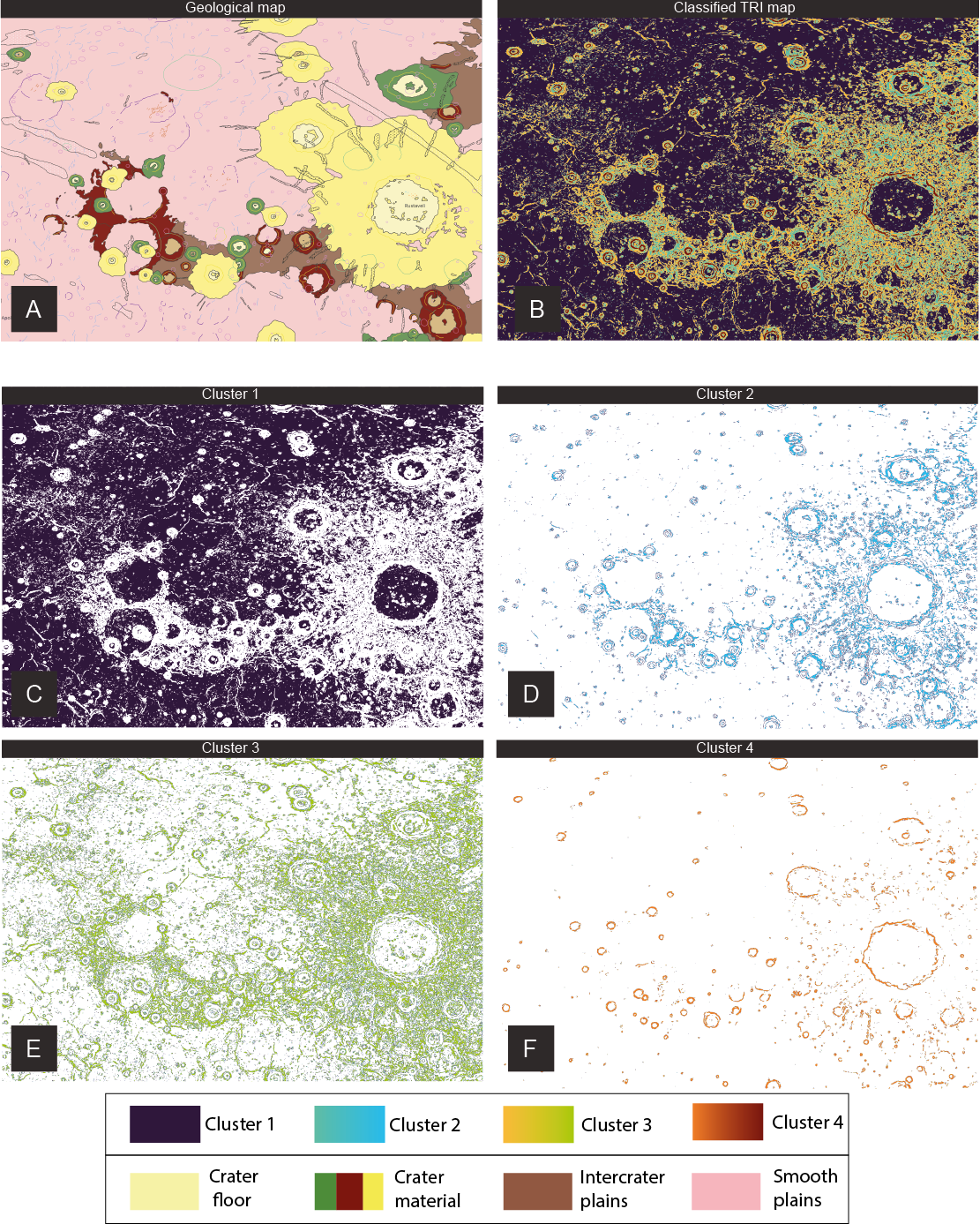
Figure 1. Preliminary clustering results with GMM applied to a TRI map of the NE section of H05 quadrangle, displaying Rustavelli crater. A. Geological map of Rustavelli crater area; B. Map of the clustering outputs showing 4 clusters; C-to-F. Maps of the identified clusters. The bottom box shows the legends for the GMM clustering (upper box) and the simplified geological units (bottom box).
Despite the absence of a performance evaluation step, the preliminary outputs already suggest the great potential of unsupervised methods to recognize geological-related features with a considerable precision. The presented outputs, together with a variety of derived maps, will be tested with different clustering algorithms and will be then evaluated by unsupervised and external metrics to evaluate quantitively the performance of the clustering algorithms.
In a near future, we hope that these exploratory maps will provide planetary geologists with an unprecedented tool for (1) refining the maps of explored terrains and (2) pioneering the mapping of new, unstudied territories by utilizing enhanced data integrating both spectral and geological information.
Acknowledgements: The study has been supported by the Italian Space Agency (ASI-INAF agreement no. 2020-17-HH.0).
References
[1] Cremonese et al. (2020). SIMBIO‐SYS: Scientific cameras and spectrometer for the BepiColombo mission. Space Science Reviews, 216(75), 75; [2] Benkhoff et al. (2021). BepiColombo-mission overview and science goals. Space Science Reviews, 217(8), 90; [3] Becker et al. (2016). First global digital elevation model of Mercury. 47th Lunar and Planetary Science Conference, Houston, TX; [4] Zambon et al. (2022). Spectral units analysis of quadrangle H05‐Hokusai on Mercury. Journal of Geophysical Research: Planets, 127(3), e2021JE006918; [5] Wright et al. (2019). Geology of the Hokusai quadrangle (H05), Mercury. Journal of Maps, 15(2), 509–520.
How to cite: Vergara Sassarini, N. A., Re, C., La Grassa, R., Tullo, A., Spina, L., and Cremonese, G.: Unsupervised classification of Mercury’s surface to aid the reconstruction of explorative geological maps., Europlanet Science Congress 2024, Berlin, Germany, 8–13 Sep 2024, EPSC2024-934, https://doi.org/10.5194/epsc2024-934, 2024.
Laser-induced breakdown spectroscopy (LIBS) is a multi-elemental analysis technique which uses laser pulses to ablate material from a target which can be located several meters away from the laser source, making the method particularly useful for in-situ planetary exploration. The first LIBS instrument employed on another planet is ChemCam which belongs to the payload of NASA’s Mars Science Laboratory (MSL) and which has been investigating the surface of Mars in Gale crater since 2012 [1, 2]. During this time and due to its regular use – almost every sol- a very large amount of data was collected: LIBS data were acquired from more than 32 000 points on Martian targets [3]. In order to obtain quantitative elemental abundances, a regression model based on the multivariate methods partial least squares regression (PLS-R) and independent component analysis (ICA) is used to predict the concentrations of the major rock forming oxides (SiO2, TiO2, Al2O3, FeOT, MgO, CaO, Na2O, K2O) by the team [4]. The model was trained on data from more than 400 standards measured on Earth with a replica instrument. This data set was also used in other studies to train for example neural networks (NN) [5]. However, this size of a dataset is still small for the training of advanced machine learning (ML) models and in general the use of supervised ML algorithms for ChemCam data is challenging due to the lack of training data from Mars. Another approach to analyze the big and diverse ChemCam LIBS dataset is to first use unsupervised techniques such as feature extraction methods followed for example by clustering, e.g. [6]. In that way it is possible to (1) identify similar targets based on their LIBS spectra and to (2) use the obtained clusters as labels and train supervised ML models. Here, we present selected unsupervised data exploration methods which have the potential to identify similar targets, dominant compositions of Mars targets measured with ChemCam and transitions between different geological units.
A LIBS measurement on a ChemCam target is typically a raster of 5–25 observation points from which each corresponds to usually 30 laser shots (i.e., 30 spectra) [7]. This allows to track chemical variability also with depth as each laser shot samples material slightly deeper than the previous one. Usually the spectra from shot 6-30 are averaged - the first 5 are omitted due to the surface dust contamination - so that one LIBS spectrum is obtained per measurement point in the raster. If these average spectra are arranged in two-dimensional matrices, they can be analyzed using matrix decomposition techniques (see schematics in Fig. 1) such as principal component analysis (PCA), non-negative matrix factorization (NMF) or ICA. They may rely on different mathematical assumptions, but in general they all return lower-dimensional matrices with so-called scores and loadings. The latter can be interpreted spectrally as they usually show emission lines from the elements similar to the original LIBS spectra, and the scores then indicate how much of each loading is present in a LIBS spectrum. Another possibility is not to average the spectra and to use the 30 spectra of a measurement point as a third dimension, so that the ChemCam data are arranged in a three-dimensional data tensor. Similar to the matrix decomposition techniques, methods from the tensor component analysis (TCA) family can be used to incorporate correlations with depth in the analysis (see schematics in Fig. 2). This can be beneficial for mineral identification based on potential correlations among elemental emission lines in successive LIBS spectra with depth, assuming that the elements primarily belong to one mineral phase.
In this study, we investigate both types of approaches the two- and three-dimensional cases for selected ChemCam LIBS datasets. The results are compared and, in particular, analyzed to figure out where the shot-to-shot analysis adds an additional insight compared to the average spectra. The data sets analyzed are mainly from the sulfate bearing unit, which is the unit that Curiosity has been driving through and investigating with its instruments for almost two Earth years now (started about sol 3700 of the mission). We focus on the general bedrock targets, which show contributions from Mg-and Ca sulfates as well as a strong Fe phase and halite [8]. In addition, when not filtered by target type, float rocks with a more Stimson like composition are also observed as a distinct group of targets [9]. A further target type appears, which is potentially a mixture of Mg and Na sulfate and is characterized by an F-bearing phase [10]. The results of both approaches applied to all these targets summarized in one dataset and to smaller sub-datasets filtered by target type will be presented.

Figure 1: Schematic of the matrix decomposition for ChemCam mean spectra. Each spectrum consists of 6144 wavelength bins, n is the number of observations included in the decomposition and R is the dimensionality of the model to be chosen.
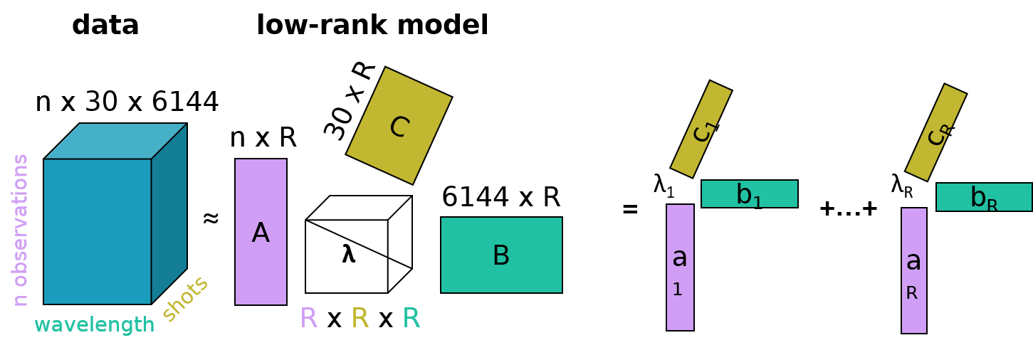
Figure 2: Schematic of TCA for ChemCam LIBS shot-to-shot data. Same meaning of n and R as in Figure 1. λ is a normalization factor so that the columns of matrices A, B, and C are all normalized to one.
References
[1] Maurice et al. (2012), SSR, 170
[2] Wiens et al. (2012), SSR, 170
[3] Gasnault (?) et al. (2024), EPSC, this meeting
[4] Clegg et al. (2017), SAPB, 129, 64
[5] Castorena et al. (2021), SAPB, 178
[6] Rammelkamp et al. (2021), EASS, 8
[7] Maurice et al. (2016), JAAS, 4
[8] Rammelkamp et al. (2024),
[9] Le Deit et al. (2024), 10th int. Mars conference
[10] Hughes et al. (2024), LPSC, #2288
How to cite: Rammelkamp, K., Gasnault, O., Schröder, S., Dehouck, E., Forni, O., Le Deit, L., Cousin, A., Lasue, J., Lomashvili, A., Hughes, E. B., and Lanza, N.: Unsupervised Data Exploration of ChemCam LIBS data from Gale crater, Mars, Europlanet Science Congress 2024, Berlin, Germany, 8–13 Sep 2024, EPSC2024-869, https://doi.org/10.5194/epsc2024-869, 2024.
Since 2012, NASA’s Curiosity rover has been looking for evidence of previous habitability on Mars [1,2]. For this purpose, the rover is equipped with a variety of scientific instruments. One of them is ChemCam (Chemistry and Camera), which consists of two parts: LIBS (Laser Induced Breakdown Spectrometer) and RMI (Remote Micro Imager). LIBS provides information on the elemental composition of targets and RMI takes context images [3]. More than 4000 targets have been measured by ChemCam since it landed [4]. One of the common questions asked when analyzing ChemCam targets is when similar targets were observed. The size of the data makes manual labeling tedious, and automating the process would reduce the human workload. In this work, we will explore machine learning methods to improve the classification process of RMI images in terms of rock texture.
In previous works, we used unsupervised classification, k-means clustering, to derive potential labels for the images [5]. We came down to nine classes: smooth, low nodular, high nodular, fractured, veins, layered, pebbles, soil, and drill shown in Fig 1. We labeled 100 images per class and used transfer learning, an already pretrained model VGG16, to make the size of the training set sufficient for convolutional neural networks [6]. The experiments showed us that more than one label applies to most ChemCam targets. This led us to multilabel classification. Although we added labels to the targets and fine-tuned models, we were not able to reach more than 80% accuracy. The model kept confusing labels, and one approach to investigate potential reasons is to employ Explainable Artificial Intelligence (XAI) methods to understand what was learned by the model. There are various methods to visualize learned patterns of each layer in deep neural networks. In order to address the so-called “black box”, we employed Guided Backpropagation [6]. The technique is a combination of backpropagation and the deconvolutional network. By setting negative gradients to zero it highlights the most activated pixels by each layer. An example of using guided backpropagation on the 10th layer of VGG16 is illustrated in Fig 2. This method allowed us to understand which textural features were learned by the model and which needed more refining.
Additionally, XAI methods are able to estimate the importance of features in the training set. Some characteristics of the image may not influence the decision-making process of the model and can be a source of extra information making the model complex and heavy. Considering the limited capacity of resources of onboard computing in in-situ missions, making models lighter is one of the priorities. Shapley values from game theory evaluates the contribution of each feature in the model that can be translated into feature importance [7]. In this work, we evaluate the feature importance of our dataset in terms of model accuracy and remove unnecessary weight from the model.
Overall, we explore multilabel classification of ChemCam targets based on their textures captured by RMIs . The automatization of labeling allows efficient interpretation of rocks and identification of regions with similar targets. We apply XAI methods such as guided backpropagation to improve the accuracy of the classification by visualizing the learned patterns. Additionally, by estimating feature importance using Shapley values, we make the model lighter for potential in-situ operation.
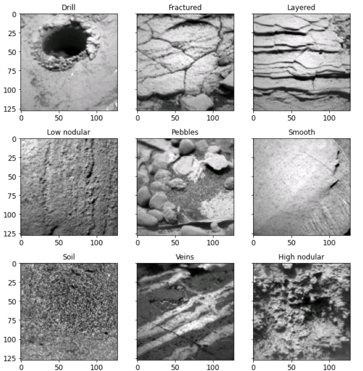
Figure 1 Representative images of the clusters and corresponding labels.
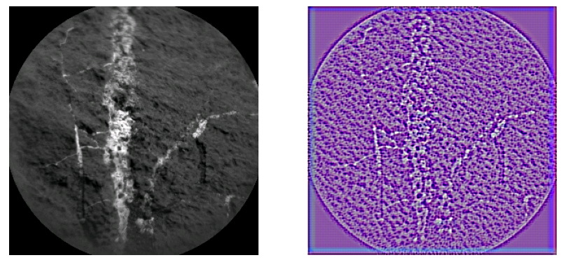
Figure 2 On the left ChemCam target "Rooibank" sol 1266, displaying veins. On the right Guided backpropagation is applied to the target, highlighting veins learned by the 10th layer of VGG16.
Refs:
[1] J. P. Grotzinger, J. Crisp, A. R. Vasavada, and R. P Anderson. Mars Science Laboratory Mission and Science Investigation. Space Sci Rev, 2012.
[2] A. R. Vasavada. Mission Overview and Scientific Contributions from the Mars Science Laboratory Curiosity Rover After Eight Years of Surface Operations. Space Sci Rev, 2022.
[3] R. C. Wiens, S. Maurice, B. Barraclough, M. Saccoccio, and W. C. Barkley. The ChemCam Instrument Suite on the Mars Science Laboratory (MSL) Rover: Body Unit and Combined System Tests. Space Sci Rev, 2012
[4] O. Gasnault et al. Exploring the sulfate-bearing unit: Recent ChemCam results at Gale crater, Mars. EPSC, 2024.
[5] A. Lomashvili et al. Rock classification via transfer learning in the scope of ChemCam RMI image data. LPSC, 2023.
[6] J. T. Springenberg, A. Dosovitskiy, T. Brox, and M. Riedmiller. Striving for Simplicity: The All Convolutional Net. ICLR 2015.
[7] S. Lundberg and S. I. Lee. A Unified Approach to Interpreting Model Predictions. NIPS 2017.
How to cite: Lomashvili, A., Rammelkamp, K., Gasnault, O., Bhattacharjee, P., Clavé, E., Egerland, C. H., and Schroeder, S.: ChemCam rock classification using explainable AI, Europlanet Science Congress 2024, Berlin, Germany, 8–13 Sep 2024, EPSC2024-780, https://doi.org/10.5194/epsc2024-780, 2024.
Introduction
Simulating thermal convection in Earth and planetary interiors is crucial for various applications, including benchmarking numerical codes (e.g. [1], [2]), deriving scaling laws for heat transfer in complex flows (e.g. [3], [4]), determining mixing efficiency (e.g. [5], [6]) and the characteristic spatial wavelengths of convection (e.g. [7]). However, reaching a statistically-steady state in these simulations, even in 2D, can be computationally expensive. While choosing "close-enough" initial conditions can significantly speed simulations up, this selection process can be challenging, especially for systems with multiple controlling parameters. This work explores how machine learning can be leveraged to identify optimal initial conditions, ultimately accelerating numerical convection simulations on their path to a statistically-steady state.
Convection model and neural network architecture
We have compiled a comprehensive dataset comprising 128 simulations of Rayleigh-Bénard convection within a rectangular domain of aspect ratio 4, characterized by variable viscosity and internal heating. A randomized parameter sweep was employed to vary three key factors: the ratio of internal heat generation to thermal driving forces (RaQ/Ra), the temperature-dependent viscosity contrast (FKT), and the pressure-dependent viscosity contrast (FKV). Each simulation was executed until the root mean square velocity and mean temperature attained a statistically stationary state. Subsequently, we extracted the time-averaged one-dimensional temperature profile, horizontally averaged across the domain, over the final 200 time steps of each simulation.

Figure 1: Schematic of the neural network used to predict statistically-steady temperature profiles.
We used a feedforward neural network (NN) to predict the 1D temperature profiles as a function of the control parameters (Fig. 1). We modified the formulation of the NN from the one we used in [8] in the following ways. First, instead of each training example consisting of the full temperature profile, we now predict temperature at a given spatial point in depth (y). This allows the network to learn and predict profiles on variable computational grids, making it more adaptable. This formulation also avoids the "wiggles" encountered when predicting high-dimensional profiles. Second, we use skip-connections. For a given hidden layer, the features from all the previous hidden layers are added to it before applying the activation function. Third, we use SELU instead of tanh for faster convergence. Fourth, we concatenate the parameters to the last hidden layer, a technique shown to improve learning in some cases (e.g., [9]). Fifth, as a consequence of conditioning the NN on spatial points, we augment the data with copies of points from the bottom and top thermal boundary layers to ensure that each batch is likely to be more representative of relevant temperature features occurring at the outer boundaries of the domain.
We split the dataset into training, cross-validation, and test sets with 96, 15, and 16 simulations, respectively. To test the extrapolation capacity of the network, we pick simulations for the test set only where at least one of the simulation parameters exceeds a certain threshold. The cross-validation dataset consists of interpolated values only and is used additionally to choose the best performing NN architecture and save network weights only when the cross-validation loss improves.
Results
We test the NN against the following baselines: linear regression, kernel ridge regression, and nearest neighbor. As shown in Table 1, when predicting unseen profiles from interpolated cases in the cross-validation set or even the extrapolated cases (Test set), the NN predictions are the most accurate among the tested possibilities. We visualize some of the profiles predicted by these algorithms in the cross-validation set in Fig. 2. Linear regression results are left out for ease of visualization.
|
Algorithm |
Training set |
Cross-validation set |
Test set |
|
Linear Regression |
0.0385 |
0.0388 |
0.0676 |
|
Kernel Ridge Regression |
0.0148 |
0.0147 |
0.0371 |
|
Neural Network |
0.0071 |
0.0071 |
0.0187 |
|
Nearest Neighbor |
0.0 |
0.0282 |
0.0495 |
Table 1: Mean absolute error of the prediction of 1D temperature profiles of statistically-steady simulations based on different tested algorithms. The lowest error per dataset is highlighted in bold.
The plots in Fig. 2 corroborate the obtained statistics about the accuracy of different methods. When the simulation parameters we are predicting happen to be close to a simulation in the training set, the nearest neighbor profile already provides a good estimate. Otherwise, the NN predictions appear to be the most accurate. This is encouraging because it shows that even for small datasets such as the one we considered, machine learning can already start delivering useful results.
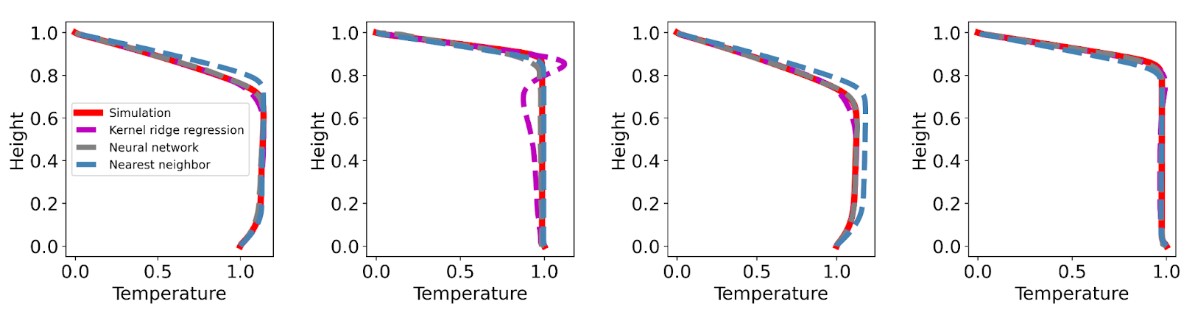
Figure 2: Four temperature profiles from the cross-validation dataset (solid red lines) and the corresponding predictions from different models (dashed lines).
Outlook
We are currently exploring how initial conditions impact the time a system takes to reach a statistically-steady state in terms of temperature and RMS velocity. We're comparing four starting points: hot, cold, linear temperature profiles, and predictions from our neural network. This will quantify the efficiency gain achieved by using the NN predictions to accelerate simulations towards equilibrium. In addition, we also plan to share the dataset and trained neural network with the community.
References
[1] King et al. (2010) A community benchmark for 2D Cartesian compressible convection in the Earth’s mantle. GJI, 180, 73-87.
[2] Tosi et al. (2015). A community benchmark for viscoplastic thermal convection in a 2-D square box. Gcubed, 16(7), 2175-2196.
[3] Vilella & Deschamps (2018). Temperature and heat flux scaling laws for isoviscous, infinite Prandtl number mixed heating convection. GJI, 214, 1, 265–281.
[4] Ferrick & Korenaga (2023). Generalizing scaling laws for mantle convection with mixed heating. JGR, 125(5), e2023JB026398.
[5] Samuel & Tosi (2012). The influence of post-perovskite strength on the Earth's mantle thermal and chemical evolution. EPSL, 323, 50-59.
[6] Thomas et al. (2014). Mixing time of heterogeneities in a buoyancy-dominated magma ocean. GJI, 236, 2, 764–777.
[7] Lenardic et al. (2006). Depth-dependent rheology and the horizontal length scale of mantle convection. JGR, 111, B7.
[8] Agarwal et al. (2020). A machine-learning-based surrogate model of Mars’ thermal evolution. GJI, 222, 3, 1656-1670.
[9] Park et al. (2019). Deepsdf: Learning continuous signed distance functions for shape representation. CVPR, 165-174.
How to cite: Agarwal, S., Tosi, N., Hüttig, C., Greenberg, D., and Bekar, A.: Determination of statistical steady states of thermal convection aided by machine learning predictions, Europlanet Science Congress 2024, Berlin, Germany, 8–13 Sep 2024, EPSC2024-394, https://doi.org/10.5194/epsc2024-394, 2024.
Accurate temperature profile estimation is a critical component in various atmospheric studies and applications, including weather forecasting, climate modeling, and atmospheric dynamics research. This study explores the potential of employing machine learning techniques to enhance temperature profile estimation by combining data from satellite and reanalysis dataset. This study attempts to leverage the strengths of both datasets by employing machine learning algorithms to develop an ensemble model that combines the high-resolution satellite measurements with the global coverage of reanalysis dataset. Specifically, the eXtreme Gradient Boosting (XGBoost) algorithm, a powerful and efficient machine learning technique, is utilized to capture the complex relationships between the variables and produce enhanced temperature profile estimates
How to cite: Ye, Q.: Attempt to Using Machine Learning Technique for Temperature Profile Estimation, Europlanet Science Congress 2024, Berlin, Germany, 8–13 Sep 2024, EPSC2024-684, https://doi.org/10.5194/epsc2024-684, 2024.
Introduction: Spectral and hyperspectral data from remote sensing instruments provide essential information on the composition of planetary surfaces. On Mars, high resolution hyperspectral data are provided by the CRISM instrument [1], onboard NASA’s MRO spacecraft. CRISM collects hyperspectral cubes in the 0.4-4 micron range, with a spectral sampling of 6.55 nm/channel and a spatial resolution up to 18.4 meter/pixel. A CRISM scene is traditionally explored through RGB maps of spectral parameters, such as band depth. To guide the user in this work, the CRISM team provided a set of 60 standard spectral parameters [2], identified based on the known spectral variability of the planet. After a first assessment with this method, extraction of single or mean spectra from selected ROIs (regions of interest) is usually performed. This is a solid approach, however, as it focuses on a few portions of the available spectral range at once, it does not fully exploit the potentials of a hyperspectral dataset. Machine Learning techniques can help us explore CRISM data more efficiently. Here we present the results from the development of a Python framework that allows the application of two different Unsupervised Learning techniques (k-Means and Gaussian Mixture Models, GMMs).
Dataset and methods: We use the CRISM Map Projected Targeted Data Records (MTRDRs) [3], the most advanced, ready-to-use CRISM dataset available. The tool has been developed in Python using the flexible and interactive Jupyter notebooks, implementing the literate programming paradigm. The clustering algorithms are taken from the Machine Learning library Scikit-Learn [4]. A combination of linear (Principal Component Analysis, PCA) and nonlinear (Uniform Manifold Approximation and Projection, UMAP) [5] dimensionality reduction techniques were employed to ensure a correct interpretation of the data structures and patterns by the algorithms. Tested combinations are listed in Table 1. In some cases, labeled with an asterisk (*), the first component of the PCA is discarded. This choice was driven by the fact that the first principal component, by capturing most of the data variance, mainly correlates with the average reflectance of the surface, often dependent on the morphology and topography of the terrain, without bearing significant mineralogical information. The quality of clustering was assessed using the Silhouette criterion [6]. The silhouette score can vary between -1 and +1, with numbers close to +1 indicating optimal clustering.
|
Combination |
Silhouette score |
|
PCA+k-Means |
0.211 |
|
PCA + GMM |
0.184 |
|
PCA* + k-Means |
0.209 |
|
PCA* + GMM |
0.195 |
|
PCA* + UMAP+ k-Means |
0.365 |
|
PCA* + UMAP + GMM |
0.357 |
Table 1: (first column) Combinations tested with the developed tool. The asterisk (*) indicates that the first principal component is discarded. (second column) Average silhouette score for 11 clusters.
Results: The methods described above have been applied to several CRISM scenes of known composition in the area of Meridiani Planum, a well-known region of Mars with a high degree of spectral variability. Both mafic [7] and aqueous mineral phases [7, 8] have been observed in the area by several authors. Here we show and discuss the results from the FRT00009B5A CRISM image covering the northern portion of Kai crater (Lat 4°20’N; lon 2°50’E). The scene has areas with mafic composition (pyroxenes), mainly outside the crater rim, and layered sediments on the crater floor, with presence of clays and sulfates. For the combinations listed in Table 1, the Silhouette coefficient indicates that the best clustering performance is achieved with 11 clusters and dimensionally reducing the data with PCA*+UMAP. In this case, the Silhouette is around 0.36 for both k-Means and GMMs, while it is around 0.2 for all the other cases. Figure 1E shows the results for k-Means clustering with PCA*+UMAP dimensionality reduction and compares them to RGB maps of spectral parameters related to either mafic or hydrous phases (Figures 1B, C, D).
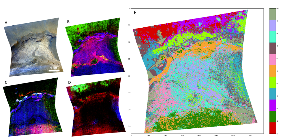
Figure 1: Comparison between RGB maps of the CRISM scene -9B5A and PCA*+UMAP+k-Means clustering. A: Image of the surface at visible wavelengths, provided for context; B: RGB map of hydrous minerals showing monohydrated (yellow) and polyhydrated (magenta) sulfates, mafic minerals (green), and clays (blue); C: RGB map of hydrous minerals showing different types of clays (white and magenta); D: RGB map of mafic minerals showing different kinds of pyroxenes (green, purple/blue areas); E: PCA*+UMAP+k-Means clustering results for 11 clusters.
Discussion and conclusions: All the main mineralogical phases present in the CRISM scene are segmented in different clusters by both algorithms. Although only the PCA*+UMAP+k-Means is shown in Figure 1, we have very similar results with GMMs. Only the monohydrated sulfate occurrences, which have a very limited spatial extension throughout the image (yellow areas in Figure 1B) are not assigned correctly in any of the tested cases listed in Table 1. However, the algorithm’s ability to capture the subtle mineralogical variations within the layered materials at the center of the scene (clusters 9 and 8, shown in lilac and aquamarine colors, in Figure 1E) is a really interesting result. These materials are known to be composed of sulfates mixed with different percentages of clay minerals [9]. Overall, k-Means and GMMs algorithms provide an interesting and valid alternative/complement for the analysis of CRISM images. We plan to apply and test the same methods shown here to other areas of Mars as well, in order to validate them on a wider range of spectral features.
Code availability: the code is fully available in the following GitHub repository: https://github.com/beatricebs/CRISM-python-unsupervised-clustering.
Acknowledgements: CRISM Data were downloaded through the PDS Geosciences Node Orbital Data Explorer (ODE). This project was supported by Fondazione Aldo Gini (University of Padova) and partially funded by Europlanet RI20-24 GMAP project (agreement No. 871149). Part of the computational resources were provided by INAF computational infrastructure for big data (DATA-STAR).
References: [1] S. Murchie et al. (2007), JGR, 112 (E5), E05S03. [2] C. E. Viviano-Beck et al. (2014), JGR Planets, 119, 1403-1431. [3] F. P. Seelos et al. (2016), LPSC XXXXVII, Abstract #1783. [4] Pedregosa, F., et al. (2011), JMLR, 12, 2825–2830, https://scikit-learn.org/stable/ [5] L. McInnes et al. (2020), https://doi.org/10.48550/arXiv.1802.03426 [6] P. J. Rousseeuw (1987), J. Comput. Appl. Math., 20, 53-65. [7] F. Poulet et al. (2008) Icarus, 195, 106-130 [8] Flahaut J. et al. (2015) Icarus, 248, 269-288. [9] Baschetti et al., “Quasiperiodic Fe/Mg clay enrichment within sulfate beds of Equatorial Layered Deposits in Meridiani Planum”, CNSP 2024.
How to cite: Baschetti, B., D'Amore, M., Carli, C., Massironi, M., and Altieri, F.: First results of Unsupervised Learning techniques applied to CRISM dataset on Mars, Europlanet Science Congress 2024, Berlin, Germany, 8–13 Sep 2024, EPSC2024-756, https://doi.org/10.5194/epsc2024-756, 2024.
Please decide on your access
Please use the buttons below to download the supplementary material or to visit the external website where the presentation is linked. Regarding the external link, please note that Copernicus Meetings cannot accept any liability for the content and the website you will visit.
Forward to presentation link
You are going to open an external link to the presentation as indicated by the authors. Copernicus Meetings cannot accept any liability for the content and the website you will visit.
We are sorry, but presentations are only available for users who registered for the conference. Thank you.
Additional speaker
- Valerio Carruba, UNESP, Brazil
Please decide on your access
Please use the buttons below to download the supplementary material or to visit the external website where the presentation is linked. Regarding the external link, please note that Copernicus Meetings cannot accept any liability for the content and the website you will visit.
Forward to session asset
You are going to open an external link to the asset as indicated by the session. Copernicus Meetings cannot accept any liability for the content and the website you will visit.
We are sorry, but presentations are only available for users who registered for the conference. Thank you.