Deep learning classification of asteroids in s-type secular resonances

Node secular resonances, or s-type secular resonances, occur when the precession frequencies of the node of an asteroid and some planets are commensurable. They are important for changing the proper inclination of asteroids interacting with them. Traditionally, identifying an asteroid's resonant status was mostly performed by visually inspecting plots of the time series of the asteroid resonant argument to check for oscillations around an equilibrium point. More recently, deep learning methods based on convolutional neural networks (CNN) for the automatic classification of images have become more popular for these kinds of tasks, allowing for the classification of thousands of orbits in a few minutes. Convolutional layers are the main component of CNNs. They apply a set of learnable filters, or convolutional kernels, to the input tensor. Each filter is a small matrix that slides over the input tensor, performing element-wise multiplication and summing the results to produce a single value.  Examples of CNN models are the Visual Geometry Group (VGG) (Simonyan & Zisserman 2014), the inception (Szegedy et al. 2015), and ResNet (He et al. 2015) models. In this work, we study 11 s-type resonances in the asteroid main belt and the Hungaria region (Knežević, 2021), and focus on the four most diffusive ones. Table (1) displays these resonances in terms of their resonant frequencies and as a combination of the arguments of linear resonances. The suffix in the frequencies identify the perturbing planet, 5 for Jupiter, 6 for Saturn, etc. The linear ν₁₆ resonance has a resonant argument s-s₆.

Resonance Identification	Res. Argument (frequencies)	Res. Argument (linear resonances)
S2	2 · s − s4 − s6	ν16 + ν14
S4	s − 2 · s6 + s7 − g6 + g8	2 · ν16 − ν17 + ν6 − ν8
S10	s − s6 − g5 + g6	ν16 + ν5 − ν6
S11	s − s6 − 2 · g5 + 2 · g6	ν16 + 2 · ν5 − 2 · ν6

Table (1): The most diffusive s-type secular resonances in the main belt, according to this study. We report the resonant argument regarding frequencies and combinations of linear secular resonances.

We selected asteroids more likely to interact with each given resonance because of their proper s values, and, by visual inspection of their resonant argument, we identified the asteroids whose resonant argument oscillated around an equilibrium point (“librating” orbits), circulates from 0^o to 360^o (“circulating” orbits) and alternated phases of circulation and libration (“switching” orbits). Since we are interested in secular effects, we can apply a low-pass filter in frequency domains, like the Butterworth filter (Butterworth 1930), to allow low-frequency signals to pass through while attenuating high-frequency signals.  Examples of asteroids on circulating and librating orbits without (left panels) and with the low-pass filter (right panels) are shown in Figure (1).

 

Figure(1): The left panels display images of the osculating resonant argument of the s-s₆+g₆−g₅ secular resonance, while the right panels do the same for the filtered arguments. 

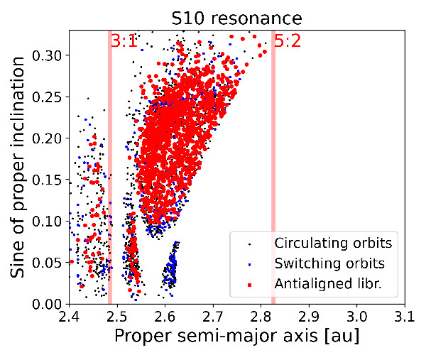
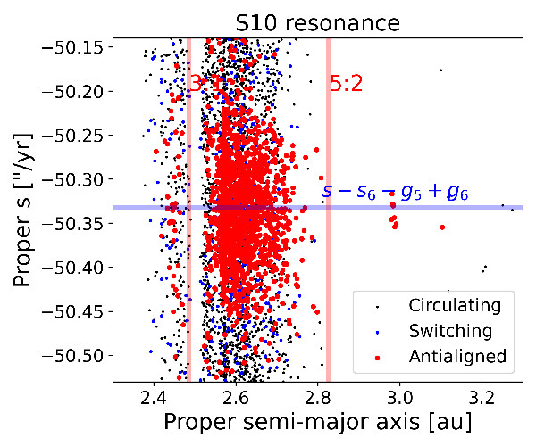
We then applied CNN models for databases of unfiltered and filtered elements and computed their efficiency using standard machine learning metrics such as accuracy, Precision, Recall, and F1-score.  Data for the S10 resonance are summarized in Table (2) and shown in Figure (2). Our results show that CNN models for filtered images are much more effective than traditional models applied to images of osculating resonant arguments.

Model	Accuracy (%)	Precision (%)	Recall (%)	F1-score (%)
VGG (U)	72	61.5	80	69.5
VGG (F)	92	86.4	95	90.5
Inception (U)	74	63	85	72.3
Inception (F)	98	95.2	100	97.6
ResNet (U)	62	51.6	80	62.7
ResNet (F)	90	90	90	90

 

Table (2): Classification in terms of accuracy, precision, recall, and F1-score for the results obtained by CNN models for samples of unfiltered (U) and filtered (F) images of the S10 resonant arguments.

 

 

Figure (2): Proper (a,sin (i)) and (a,s) projections of numbered asteroids with errors in proper s < 0.2 arcsec yr⁻¹ for bodies in the S10 resonance. 

 

Filtered resonant arguments should be preferentially used to identify asteroids interacting with secular resonances. This work is currently under consideration by MNRAS. 

References

Butterworth S., 1930, Wireless Engineer, 7, 536.

Carruba V., et al. 2021, CMDA, 133, 38.

Carruba V. et al. 2024, MNRAS, submitted.

He K., Zhang X., Ren S., Sun J., 2015, Deep Residual Learning for Image Recognition, doi:10.48550/ARXIV.1512.03385, https://arxiv.org/abs/1512.03385

Knežević Z., 2021, Serbian Academy of Sciences and Arts.

Lyapunov A. 1892, Annals of Mathematics and Mechanics, 17, 1.

Simonyan K., Zisserman A., 2014, arXiv e-prints, p. arXiv:1409.1556.

Szegedy C., et al., 2015, in Proceedings of the IEEE conference on computer vision and pattern recognition. pp 1–9.