Determination of statistical steady states of thermal convection aided by machine learning predictions

Introduction

Simulating thermal convection in Earth and planetary interiors is crucial for various applications, including benchmarking numerical codes (e.g. [1], [2]), deriving scaling laws for heat transfer in complex flows (e.g. [3], [4]), determining mixing efficiency (e.g. [5], [6]) and the characteristic spatial wavelengths of convection (e.g. [7]). However, reaching a statistically-steady state in these simulations, even in 2D, can be computationally expensive. While choosing "close-enough" initial conditions can significantly speed simulations up, this selection process can be challenging, especially for systems with multiple controlling parameters. This work explores how machine learning can be leveraged to identify optimal initial conditions, ultimately accelerating numerical convection simulations on their path to a statistically-steady state.

Convection model and neural network architecture

We have compiled a comprehensive dataset comprising 128 simulations of Rayleigh-Bénard convection within a rectangular domain of aspect ratio 4, characterized by variable viscosity and internal heating. A randomized parameter sweep was employed to vary three key factors: the ratio of internal heat generation to thermal driving forces (RaQ/Ra), the temperature-dependent viscosity contrast (FKT), and the pressure-dependent viscosity contrast (FKV). Each simulation was executed until the root mean square velocity and mean temperature attained a statistically stationary state. Subsequently, we extracted the time-averaged one-dimensional temperature profile, horizontally averaged across the domain, over the final 200 time steps of each simulation.

Figure 1: Schematic of the neural network used to predict statistically-steady temperature profiles.

We used a feedforward neural network (NN) to predict the 1D temperature profiles as a function of the control parameters (Fig. 1). We modified the formulation of the NN from the one we used in [8] in the following ways. First, instead of each training example consisting of the full temperature profile, we now predict temperature at a given spatial point in depth (y). This allows the network to learn and predict profiles on variable computational grids, making it more adaptable. This formulation also avoids the "wiggles" encountered when predicting high-dimensional profiles. Second, we use skip-connections. For a given hidden layer, the features from all the previous hidden layers are added to it before applying the activation function. Third, we use SELU instead of tanh for faster convergence. Fourth, we concatenate the parameters to the last hidden layer, a technique shown to improve learning in some cases  (e.g., [9]). Fifth, as a consequence of conditioning the NN on spatial points, we augment the data with copies of points from the bottom and top thermal boundary layers to ensure that each batch is likely to be more representative of relevant temperature features occurring at the outer boundaries of the domain. 

We split the dataset into training, cross-validation, and test sets with 96, 15, and 16 simulations, respectively. To test the extrapolation capacity of the network, we pick simulations for the test set only where at least one of the simulation parameters exceeds a certain threshold. The cross-validation dataset consists of interpolated values only and is used additionally to choose the best performing NN architecture and save network weights only when the cross-validation loss improves. 

Results

We test the NN against the following baselines: linear regression, kernel ridge regression, and nearest neighbor. As shown in Table 1, when predicting unseen profiles from interpolated cases in the cross-validation set or even the extrapolated cases (Test set), the NN predictions are the most accurate among the tested possibilities. We visualize some of the profiles predicted by these algorithms in the cross-validation set in Fig. 2. Linear regression results are left out for ease of visualization. 

Algorithm	Training set	Cross-validation set	Test set
Linear Regression	0.0385	0.0388	0.0676
Kernel Ridge Regression	0.0148	0.0147	0.0371
Neural Network	0.0071	0.0071	0.0187
Nearest Neighbor	0.0	0.0282	0.0495

Table 1: Mean absolute error of the prediction of 1D temperature profiles of statistically-steady simulations based on different tested algorithms. The lowest error per dataset is highlighted in bold.

The plots in Fig. 2 corroborate the obtained statistics about the accuracy of different methods. When the simulation parameters we are predicting happen to be close to a simulation in the training set, the nearest neighbor profile already provides a good estimate. Otherwise, the NN predictions appear to be the most accurate. This is encouraging because it shows that even for small datasets such as the one we considered, machine learning can already start delivering useful results. 

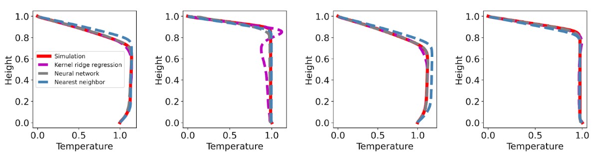
Figure 2: Four temperature profiles from the cross-validation dataset (solid red lines) and the corresponding predictions from different models (dashed lines).

Outlook

We are currently exploring how initial conditions impact the time a system takes to reach a statistically-steady state in terms of temperature and RMS velocity. We're comparing four starting points: hot, cold, linear temperature profiles, and predictions from our neural network. This will quantify the efficiency gain achieved by using the NN predictions to accelerate simulations towards equilibrium. In addition, we also plan to share the dataset and trained neural network with the community.

References

[1] King et al. (2010) A community benchmark for 2D Cartesian compressible convection in the Earth’s mantle. GJI,  180, 73-87.

[2] Tosi et al. (2015).  A community benchmark for viscoplastic thermal convection in a 2-D square box. Gcubed, 16(7), 2175-2196.

[3] Vilella & Deschamps (2018). Temperature and heat flux scaling laws for isoviscous, infinite Prandtl number mixed heating convection. GJI, 214, 1, 265–281.

[4] Ferrick & Korenaga (2023). Generalizing scaling laws for mantle convection with mixed heating. JGR, 125(5), e2023JB026398.

[5] Samuel & Tosi (2012). The influence of post-perovskite strength on the Earth's mantle thermal and chemical evolution. EPSL, 323, 50-59.

[6] Thomas et al. (2014). Mixing time of heterogeneities in a buoyancy-dominated magma ocean. GJI, 236, 2, 764–777.

[7] Lenardic et al. (2006). Depth-dependent rheology and the horizontal length scale of mantle convection. JGR, 111, B7.

[8] Agarwal et al. (2020). A machine-learning-based surrogate model of Mars’ thermal evolution. GJI, 222, 3, 1656-1670.

[9] Park et al. (2019). Deepsdf: Learning continuous signed distance functions for shape representation. CVPR, 165-174.