First results of Unsupervised Learning techniques applied to CRISM dataset on Mars

Introduction: Spectral and hyperspectral data from remote sensing instruments provide essential information on the composition of planetary surfaces. On Mars, high resolution hyperspectral data are provided by the CRISM instrument [1], onboard NASA’s MRO spacecraft. CRISM collects hyperspectral cubes in the 0.4-4 micron range, with a spectral sampling of 6.55 nm/channel and a spatial resolution up to 18.4 meter/pixel. A CRISM scene is traditionally explored through RGB maps of spectral parameters, such as band depth. To guide the user in this work, the CRISM team provided a set of 60 standard spectral parameters [2], identified based on the known spectral variability of the planet. After a first assessment with this method, extraction of single or mean spectra from selected ROIs (regions of interest) is usually performed. This is a solid approach, however, as it focuses on a few portions of the available spectral range at once, it does not fully exploit the potentials of a hyperspectral dataset. Machine Learning techniques can help us explore CRISM data more efficiently. Here we present the results from the development of a Python framework that allows the application of two different Unsupervised Learning techniques (k-Means and Gaussian Mixture Models, GMMs). 

Dataset and methods: We use the CRISM Map Projected Targeted Data Records (MTRDRs) [3], the most advanced, ready-to-use CRISM dataset available. The tool has been developed in Python using the flexible and interactive Jupyter notebooks, implementing the literate programming paradigm. The clustering algorithms are taken from the Machine Learning library Scikit-Learn [4]. A combination of linear (Principal Component Analysis, PCA) and nonlinear (Uniform Manifold Approximation and Projection, UMAP) [5] dimensionality reduction techniques were employed to ensure a correct interpretation of the data structures and patterns by the algorithms. Tested combinations are listed in Table 1. In some cases, labeled with an asterisk (*), the first component of the PCA is discarded. This choice was driven by the fact that the first principal component, by capturing most of the data variance, mainly correlates with the average reflectance of the surface, often dependent on the morphology and topography of the terrain, without bearing significant mineralogical information. The quality of clustering was assessed using the Silhouette criterion [6]. The silhouette score can vary between -1 and +1, with numbers close to +1 indicating optimal clustering.

Combination	Silhouette score
PCA+k-Means	0.211
PCA + GMM	0.184
PCA* + k-Means	0.209
PCA* + GMM	0.195
PCA* + UMAP+  k-Means	0.365
PCA* + UMAP + GMM	0.357

Table 1: (first column) Combinations tested with the developed tool. The asterisk (*) indicates that the first principal component is discarded. (second column) Average silhouette score for 11 clusters. 

Results: The methods described above have been applied to several CRISM scenes of known composition in the area of Meridiani Planum, a well-known region of Mars with a high degree of spectral variability. Both mafic [7] and aqueous mineral phases [7, 8] have been observed in the area by several authors. Here we show and discuss the results from the FRT00009B5A CRISM image covering the northern portion of Kai crater (Lat 4°20’N; lon 2°50’E). The scene has areas with mafic composition (pyroxenes), mainly outside the crater rim, and layered sediments on the crater floor, with presence of clays and sulfates. For the combinations listed in Table 1, the Silhouette coefficient indicates that the best clustering performance is achieved with 11 clusters and  dimensionally reducing the data with PCA*+UMAP. In this case, the Silhouette is around 0.36 for both k-Means and GMMs, while it is around 0.2 for all the other cases. Figure 1E shows the results for k-Means clustering with PCA*+UMAP dimensionality reduction and compares them to RGB maps of spectral parameters related to either mafic or hydrous phases (Figures 1B, C, D). 

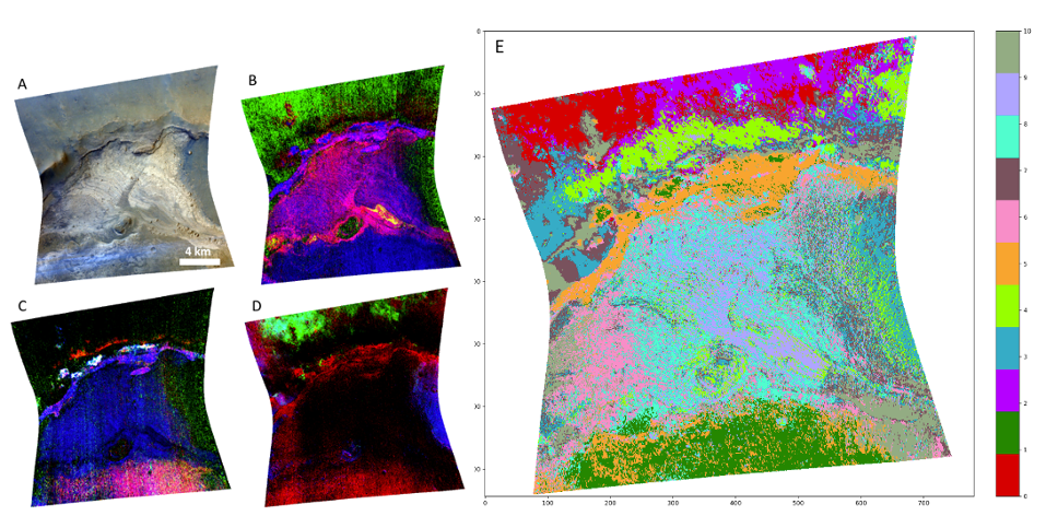
Figure 1: Comparison between RGB maps of the CRISM scene -9B5A and PCA*+UMAP+k-Means clustering. A: Image of the surface at visible wavelengths, provided for context; B: RGB map of hydrous minerals showing monohydrated (yellow) and polyhydrated (magenta) sulfates, mafic minerals (green), and clays (blue); C: RGB map of hydrous minerals showing different types of clays (white and magenta); D: RGB map of mafic minerals showing different kinds of pyroxenes (green, purple/blue areas); E: PCA*+UMAP+k-Means clustering results for 11 clusters. 

Discussion and conclusions: All the main mineralogical phases present in the CRISM scene are segmented in different clusters by both algorithms. Although only the PCA*+UMAP+k-Means is shown in Figure 1, we have very similar results with GMMs. Only the monohydrated sulfate occurrences, which have a very limited spatial extension throughout the image (yellow areas in Figure 1B) are not assigned correctly in any of the tested cases listed in Table 1. However, the algorithm’s ability to capture the subtle mineralogical variations within the layered materials at the center of the scene (clusters 9 and 8, shown in lilac and aquamarine colors, in Figure 1E) is a really interesting result. These materials are known to be composed of sulfates mixed with different percentages of clay minerals [9]. Overall, k-Means and GMMs algorithms provide an interesting and valid alternative/complement for the analysis of CRISM images. We plan to apply and test the same methods shown here to other areas of Mars as well, in order to validate them on a wider range of spectral features.

Code availability: the code is fully available in the following GitHub repository: https://github.com/beatricebs/CRISM-python-unsupervised-clustering. 

Acknowledgements: CRISM Data were downloaded through the PDS Geosciences Node Orbital Data Explorer (ODE). This project was supported by Fondazione Aldo Gini (University of Padova) and partially funded by Europlanet RI20-24 GMAP project (agreement No. 871149). Part of the computational resources were provided by INAF computational infrastructure for big data (DATA-STAR).

References: [1] S. Murchie et al. (2007), JGR, 112 (E5), E05S03. [2] C. E. Viviano-Beck et al. (2014), JGR Planets, 119, 1403-1431. [3] F. P. Seelos et al. (2016), LPSC XXXXVII, Abstract #1783. [4] Pedregosa, F., et al. (2011), JMLR, 12, 2825–2830, https://scikit-learn.org/stable/ [5] L. McInnes et al. (2020), https://doi.org/10.48550/arXiv.1802.03426 [6] P. J. Rousseeuw (1987), J. Comput. Appl. Math., 20, 53-65. [7] F. Poulet et al. (2008) Icarus, 195, 106-130 [8] Flahaut J. et al. (2015) Icarus, 248, 269-288. [9] Baschetti et al., “Quasiperiodic Fe/Mg clay enrichment within sulfate beds of Equatorial Layered Deposits in Meridiani Planum”, CNSP 2024.