A Conditional Neural Autoencoder for Haze Microphysics Modeling in Exoplanet Atmospheres

Simulating exoplanetary atmospheres is essential for characterizing their composition, hazes, clouds, and observational signatures. With the emergence of JWST (James Webb Space Telescope) and the upcoming ARIEL (Atmospheric Remote-sensing Infrared Exoplanet Large-survey) mission [8,9], the need for a fast implementation of classical forward models is increasing. Machine learning (ML) can address this by providing surrogate models that approximate selected model components and accelerate the simulation pipeline. In our research, we use a 1D, self-consistent forward model (FM) coupling stellar energy deposition, disequilibrium chemistry, and haze/cloud microphysics from the deep atmosphere (10³ bar) to the upper thermosphere (~10^-¹⁰ bar) [1,2,7]. Here, we aim to develop a supervised neural-network surrogate model, inspired by previous ML applications [4], trained on the outputs of the FM and capable of rapidly approximating atmospheric responses over a range of parameters, including planetary mass, temperature-pressure structure, metallicity, gravity, and stellar flux, without repeated execution of the full model.

As a first step, we focus on the haze-microphysics component of the FM, a controlled test case before extending the method to more strongly coupled processes such as radiative transfer and disequilibrium chemistry. The haze module evolves the vertical distribution of particles through monomer production, coagulation, eddy diffusion, and gravitational settling, producing haze mixing-ratio profiles over a fixed pressure grid and multiple particle-size bins [6]. We first consider an isothermal setup, where temperature is constant throughout the atmospheric column, to isolate the ML model’s ability to learn the dependence of haze profiles on the main physical parameters. Synthetic training and validation datasets are generated by repeatedly running the isolated haze module for different isothermal temperatures (Tiso = 300–1400 K), constant eddy diffusion, and planetary mass scaling.

The resulting neural-network model, trained on isothermal structures and hereafter called the ISO model, combines encoders designed to simplify the physical structure of the problem. A temperature projection is used for the scalar thermal input, a pressure autoencoder compresses the vertical pressure grid, and species-specific LSTM (Long Short-Term Memory) autoencoders encode the vertical haze mixing-ratio profiles. These latent representations are combined in a core neural network that learns the coupling between atmospheric conditions and haze-species distributions before reconstructing the predicted profiles through decoder and denoising layers. The ISO model reproduces the main structure of the FM haze profiles, including the production region and general vertical behavior of the haze distribution (fig. 1a-f). The best agreement is obtained for small and intermediate particle-size bins and intermediate temperatures, while larger particles and the temperature-range edges remain more challenging. Sensitivity tests show that the model captures the dominant haze-profile response to variations in planetary mass scaling and eddy diffusion (fig. 1g-l).

To move towards more realistic atmospheres, we introduce a fine-tuning step based on non-isothermal temperature-pressure (TP) profiles and their corresponding haze-mixing ratios calculated by the FM. Instead of replacing the isothermal model completely, the TP profile is decomposed into a mean reference temperature and a vertical temperature-deviation profile. The mean temperature represents the closest isothermal approximation to the atmosphere, allowing the model to retain the haze-microphysics behavior already learned by the ISO model. The deviation profile, ΔT(P), provides information on how much the real atmosphere deviates from this approximation at each pressure level and is then embedded in the total temperature latent space. The temperature-deviation profile is encoded using one-dimensional convolutional layers, which are well suited to ordered vertical profiles because they can identify local thermal structures along the atmospheric column [3,5]. In this way, the fine-tuned model introduces pressure-dependent thermal information into the latent space while preserving the pretrained isothermal representation, enabling the predicted haze profiles to respond more realistically to non-isothermal atmospheric conditions.

The fine-tuned model performs better than the original ISO model (fig. 2b,c,e), but it does not fully predict all non-isothermal cases. Adding TP information helps, especially for the main haze region and for smaller/intermediate particles, but the neural network still struggles when the atmosphere differs strongly from the original isothermal training cases (fig. 2d,f,g). This fine-tuning step therefore represents an intermediate stage toward a future model trained directly on fully non-isothermal atmospheres, which will be our next approach.

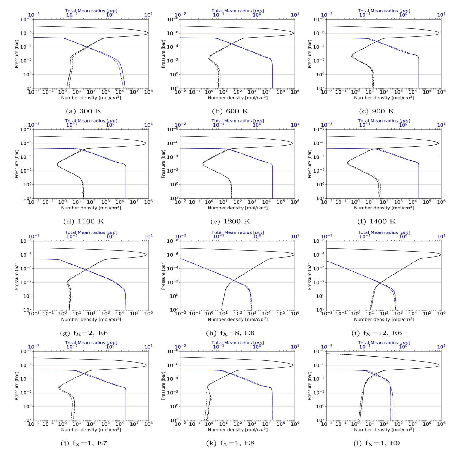
Figure 1: Comparison of the ISO model’s predictions (solid lines) with the calculations by the isolated-FM (dashed lines). (a)–(f): Temperature sensitivity test: each subplot is a summarized representation of all the available haze species, the number density (black lines) and total mean radius (blue lines), in the atmosphere, under f_X = 1 (planetary mass scaling factor) and eddy diffusion coefficient 10⁶ cm²/s. (g)–(l): Mass scaling and eddy sensitivity test:each subplot shows the ISO model versus the FM by varying the f_X and the eddy diffusion coefficient, e.g. E6 is 10⁶ cm²/s, under the same isothermal temperature 900 K.

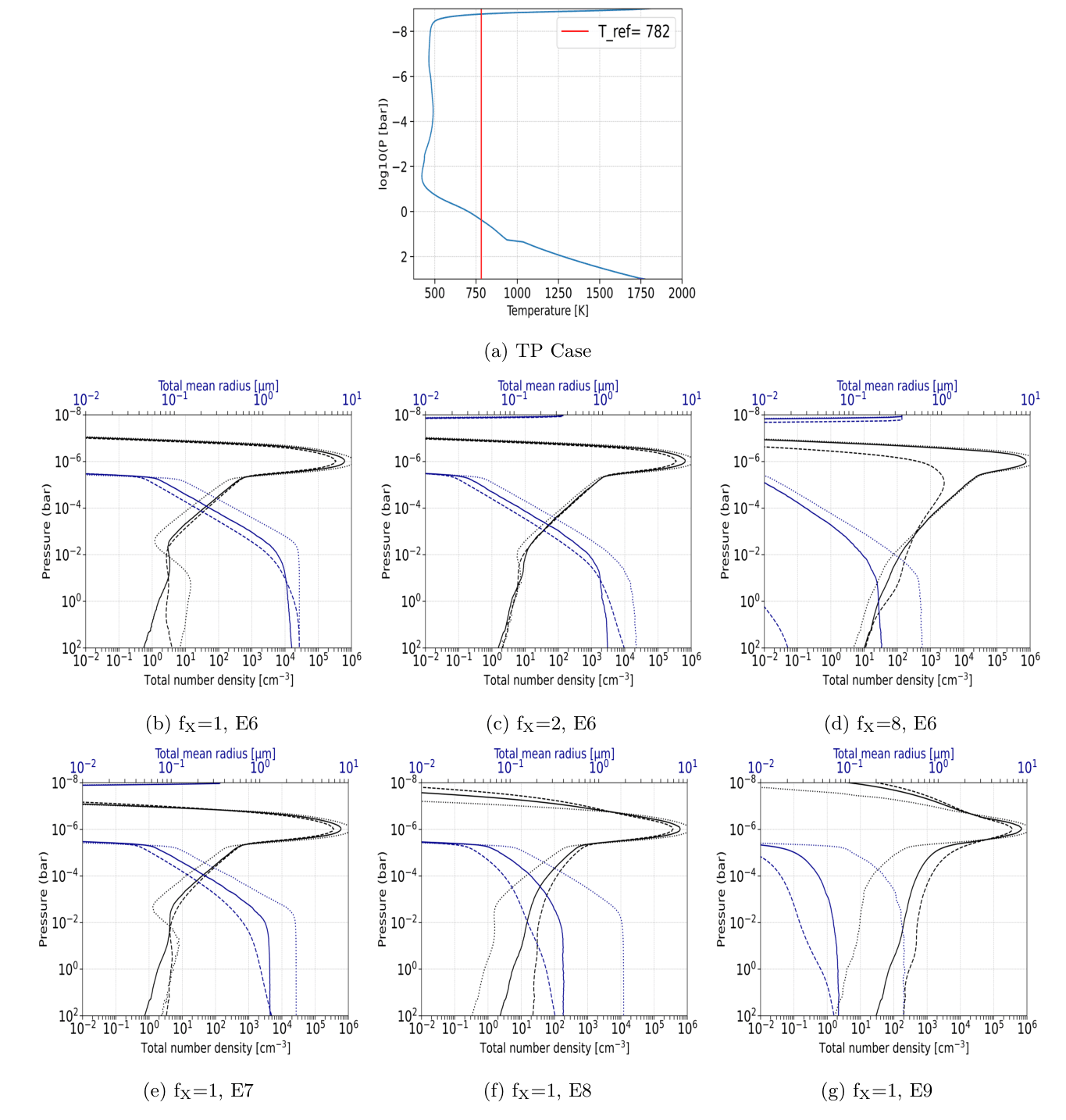
Figure 2: Top panel:  TP profile that was used for the FM calculations. The red line indicates the reference isothermal temperature that was used for the prediction of the ISO model. Bottom plots: the corresponding average properties of the atmosphere, as a function of pressure. Plots (b) to (g) compare the TP-finetuned version (solid lines) with the FM solution (dashed) and the isothermal prior (dotted) predictions.

References

[1] A. Arfaux et al. Monthly Notices of the Royal Astronomical Society 515.4 (2022), pp. 4753–4779. doi: 10.1093/mnras/stac1772.

[2] A. Arfaux et al. Monthly Notices of the Royal Astronomical Society 522.2 (2023), pp. 2525–2542. doi: 10.1093/mnras/stad1135.

[3] S. Bai et al. arXiv e-prints (2018), arXiv:1803.01271. doi: 10.48550/arXiv.1803.01271.

[4] J. L. A. M. Hendrix et al. Monthly Notices of the Royal Astronomical Society 524.1 (2023), pp. 643–655. doi: 10.1093/mnras/stad1763.

[5] S. Kiranyaz et al. Mechanical Systems and Signal Processing 151 (2021), p. 107398. doi: 10.1016/j.ymssp.2020.107398.

[6] P. Lavvas et al. The Astrophysical Journal 847.1 (2017), p. 32. doi: 10.3847/1538-4357/aa88ce.

[7] P. Lavvas et al. The Astrophysical Journal 878.2 (2019), p. 118. doi: 10.3847/1538-4357/ab204e.

[8] E. Pascale et al. Space Telescopes and Instrumentation 2018: Optical, Infrared, and Millimeter Wave. Vol. 10698. SPIE Conference Series. 2018, 106980H. doi: 10.1117/12.2311838.

[9] G. Tinetti et al. Experimental Astronomy 46.1 (2018), pp. 135–209. doi: 10.1007/s10686-018-9598-x.