Loki Patera’s specular surface by JunoCam image data

During Juno’s approach to Perijove 58, her wide-angle visible light imager JunoCam took a sequence of Io images. Four of those images show the lava lake Loki Patera with a solar specular deviation angle varying approximately between 0.25 and 0.8 radians.

We call the angle between the solar specular vector relative to Io’s nominal surface normal and the vector from the respective surface point to the camera the solar specular deviation angle. We call the angle between the plane defined by the sun and the respective surface normal solar specular azimuth when seen relative to the solar specular vector. This construct is similar to polar azimuthal coordinates, just with the solar specular vector as symmetry axis, and the vector to the Sun being used to define the zero azimuth.

We sample an annulus around the lava lake in order to estimate relative exposure times and dark biases by applying linear least-square regression. This approach is described in Figure 1.

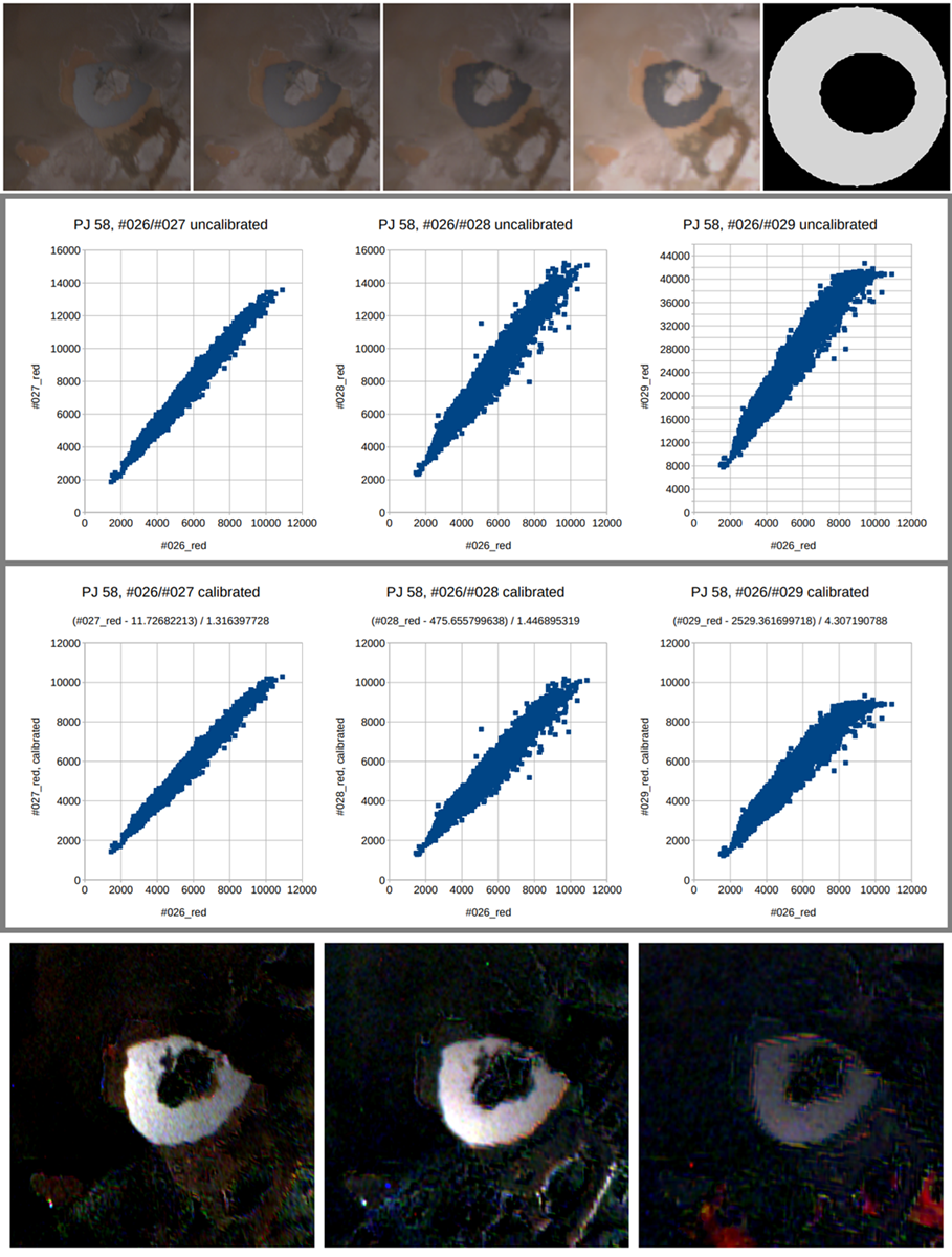
Figure 1: Crops of cylindrical map projections of the four JunoCam images 26, 27, 28, and 29 taken before Perijove 58 are shown in the first row, together with a mask that defines an annular area around the lava lake of Loki Patera. North is to the right. Samples within this annulus are taken for images 27, 28, and 29, and brightness-correlated to the same locations in image 26. The second row shows the resulting correlation diagrams. Linear least-square regression is applied to those data sets as an approximation of a calibration of images 27, 28, and 29 relative to image 26. The resulting calibrated correlation is shown in the third row. The fourth row shows the residuals betweem consecutive images, hence for image pairs (26-27), (27-28), and (28-29).

The residuals remove most of the area outside the lava lakes. The lava lakes themselves show up very distinctly. We use this property for image pair (26-27) together with the red/green slope of image 26, and with a draft elliptical area selection, as a heuristics to define a mask that covers the lava lake. This mask is then further eroded in order to make sure that sampling within the mask does contain only interior points of the lava lake area, see Figure 2.

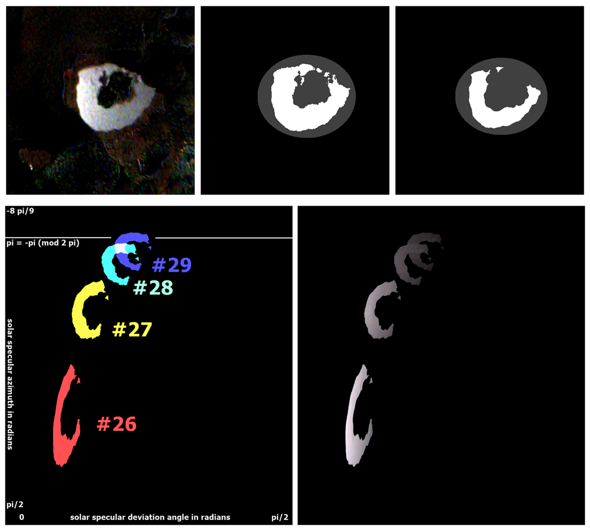
Figure 2: The first row visualizes steps from the difference (26-27) of calibrated images 26 and 27, over a mask that covers the lava lake area, to an eroded mask that covers only the interior area of Loki Patera. The second row plots the mask and the masked and calibrated caldera in coordinates of the solar specular deviation angle and azimuth, both in radians, and applied to all four considered images. Since the Juno spacecraft is changing her position with each image, the lava lake changes its apparent position relative to the solar specular vector. Compared to the surrounding area of the lava lake, its interor area is brightest for image 26, and dims until image 29, while the solar specular deviation angle is increasing. The y axis at the left border of the two panels at the bottom defines the solar specular vector, along which a perfect spherical mirror with Io’s radius and center would reflect the sunlight.

 

With this prerequisites, we sample Loki Patera along contour lines of either constant solar specular deviation angle, or of constant solar specular azimuth. Sampling is restricted to the eroded mask in order to retrieve only valid samples from the interior of the lava lake area. Both cases are visualized in Figure 3.

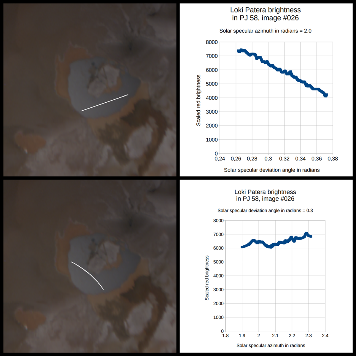
Figure 3: The first row samples along the contour line with a solar specular azimuth equal to 3.0 radians. The second row samples along the line with a specular deviation angle of 0.3 radians. The left column shows the sampling tracks in cylindrical map projections. The right column shows the brightness charts of the red channel. The effect of the solar specular deviation angle is significant and locally close to linear, while the effect of the azimuth can be interpreted as weakly linear, not quite constant, and noisy, or influenced by local heterogeneities.

Samples taken along contour lines suggest that brightness values of the lava lake can be reasonably approximated patera-locally, and for each image separately by linear regression over two dimensions with the solar specular deviation angle and azimuth as axes.

Concavity of the brightness plot becomes apparent only after combining charts of a sequence of images.