Poster presentations and abstracts

The Great Red Spot (GRS) of Jupiter is a large anticyclonic vortex present in the Jovian atmosphere. First observed in the XVII century, it is almost constantly located at 22°S. Since its discovery it has gradually decreased in size at an average rate of 170 km/year in longitude and 60 km/year in latitude. The nature of the chromophore species that provide its characteristic color to the GRS’s upper clouds and hazes is still largely unknown, as well as its creation and destruction mechanisms. During year 2019, the GRS began to lose some of this reddish material as a consequence of the interaction with other vortices present in nearby latitudes, raising serious doubts about its possible disappearance (Sánchez-Lavega et al., 2019).

In this work we have analyzed images provided by the Hubble Space Telescope between 2015 and 2019, with a spectral coverage from the ultraviolet to the near infrared, including some methane absorption bands of different depths. These images have been calibrated in absolute reflectivity, and from them we have obtained the spectral variations in brightness that occur in different dynamically interesting regions of the GRS and its surroundings.

The spectral reflectivity of the studied regions over the mentioned years has been analyzed using the NEMESIS radiative transfer code (Irwin et al., 2008). In this way it has been possible to retrieve the main features playing a key role in the spectral reflectivity of GRS’s upper clouds and hazes, such as particle size distribution, refractive indexes and optical thickness. At the same time, this analysis has provided the vertical distribution of particles for pressure levels above 1 bar, allowing a comparative study of its evolution over recent years.

References

-Irwin, P. G. J., Teanby, N. A., de Kok, R., Fletcher, L. N., Howett, C. J. A., Tsang, C. C. C., . . . Parrish, P. D. (2008, April). The NEMESIS planetary atmosphere radiative transfer and retrieval tool. Journal of Quant. Spec. and Radiative Transfer, 109, 1136-1150. doi: 10.1016/j.jqsrt.2007.11.006

- Sánchez-Lavega, A., Iñurrigarro, P., Anguiano-Arteaga, A., Garcia-Melendo, E., Legarreta, J., Hueso, R., Sanz-Requena, J.F., Pérez-Hoyos, S.,  Mendikoa, I., Soria, M., Rojas, J.F. Jupiter’s Great Red Spot threatened along 2019 by strong interactions with close anticyclones, AGU Fall Meeting, P44A-01, San Francisco, 12 December 2019

How to cite: Anguiano-Arteaga, A., Pérez-Hoyos, S., and Sánchez-Lavega, A.: Variations in spectral reflectivity and vertical cloud structure of Jupiter’s Great Red Spot, Europlanet Science Congress 2020, online, 21 Sep–9 Oct 2020, EPSC2020-209, https://doi.org/10.5194/epsc2020-209, 2020.

Transit observations reveal that a significant population of the detected exoplanets has hazy atmospheres (Sing et al. 2016). Although the relative contribution of clouds and photochemical aerosols is not yet fully clarified, the impact of haze particles on the thermal structure could be significant, as such particles can efficiently scatter and absorb radiation over a large part of the electromagnetic spectrum. Particularly, photochemical aerosols are anticipated to be present at pressures lower than those of cloud formation. The transit observations of HD 189733 b indicate that the haze opacity responsible for the UV-Visible slope is located at pressures between 1μbar and 1 mbar. As such low pressures, the presence of hazes could allow for strong temperature inversions due to the low atmospheric density. We investigate here the implications of such hazes on the exoplanet atmospheric thermal structure.

We simulate the atmospheric thermal structure using a 1D radiative-convective model. The model utilizes non-equilibrium chemical composition results (Lavvas et al. 2014) for the gas phase composition, and haze particle size distributions calculated from an aerosol microphysical growth model (Lavvas & Koskinen 2017, Lavvas et al. 2019). We do not yet consider the non-LTE effects for the gases, but we do take into account the impact of temperature disequilibrium between the particles and the gas envelope that can strongly affect the heating efficiency of the particles. We consider various gas phase opacities from atomic and molecular contributions calculated through correlated-k coefficients.

Our results demonstrate that in the lower atmosphere the simulated temperature profiles provide emission spectra that are in good agreement with the eclipse observations for the simulated targets (HD 209458 b and HD 189733 b). In the upper atmosphere of the hazy HD 189733 b the simulated haze distribution, which fits the transit observations, results in a strong temperature inversion. On the contrary, the upper atmosphere of the clear HD 209458 b, is significantly colder compared to previous evaluations based on equilibrium chemistry assumption. The implications of these results on the chemical composition will be discussed, as well as results from other exoplanet cases.

How to cite: Lavvas, P. and Arfaux, A.: Impact of photochemical hazes on the thermal structure of exoplanet atmospheres, Europlanet Science Congress 2020, online, 21 Sep–9 Oct 2020, EPSC2020-461, https://doi.org/10.5194/epsc2020-461, 2020.

Introduction

The martian atmosphere is mainly composed of CO₂ (~ 95 %). The first spectral confirmation of CO₂ cloud was acquired by Montmessin et al. [2007] using the 4.26 µm band of the ν₃ fundamental asymmetric stretching mode of CO₂ from OMEGA data onboard Mars Express. 

Since then, numerous observational studies have constrained the climatology of CO₂ cloud in the martian atmosphere [Määttänen et al., 2013]. There are two different types of clouds involving different formation processes: (i) those located in the troposphere at the winter polar region, and (ii) those located in the mesosphere at low and mid-latitudes during the martian year [Määttänen et al., 2013]. Microphysical processes of formation of theses clouds are still not fully understood. However, modeling studies revealed processes necessary for their formation: the requirement of waves that perturb the atmosphere leading to a temperature below the condensation of CO₂ (transient planetary waves for tropospheric clouds [Kuroda et al., 2013], thermal tides [Gonzàlez-Galindo et al., 2011] and gravity waves for mesospheric clouds [Spiga et al., 2012]).

We use our microphysical model of CO₂ cloud formation to investigate the occurrence of these CO₂ cloud by coupling it with the Global Climate Model (GCM) of the Institut Pierre Simon Laplace (IPSL) [Forget et al., 1999]. We focus our efforts on the modeling of the tropospheric clouds during the winter in the polar regions.

Model description

The microphysical model of CO₂ cloud formation of LATMOS includes nucleation on crystals on cloud condensation nuclei (CCN), condensation/sublimation, and sedimentation. Sources of CCN for CO₂ are mainly dust particles, secondarily water ice particles. The particle size distribution is described with the moment method allowing to compute the effect of the microphysical processes on the average properties of the distribution. This method is the same as used for water ice clouds microphysics in the MGCM-IPSL [Madeleine et al., 2014, Navarro et al., 2014]. For more details about the microphysical processes of CO₂ clouds, we invite the reader to the work of Listowski et al. [2013, 2014].

The MGCM-IPSL is a finite difference model based on the primitive equations of meteorology in σ coordinates [Forget et al., 1999]. The horizontal resolution grid used is 64 x 48, corresponding to 5.6258° longitude by 3.758° latitude, respectively. The top of the atmosphere was extended to ~ 120 km to describe well the processes in the mesosphere. The atmosphere is divided into 32 vertical layers from the surface to the top of the atmosphere. At each call of physical processes (every 15 minutes), the microphysics of CO₂ cloud formation is called 50 times leading to a time resolution of 18 seconds to resolve the very rapid microphysical processes. We have used a dust scenario from the MY29.

Results

We present our first results on 3D modeling CO₂ clouds in the Martian atmosphere. Figure 1 shows the zonal mean density column of atmospheric CO₂ ice as simulated by the model during a Martian year. The maximum columns of CO₂ clouds are found in winter polar regions. In the northern polar region, CO₂ ice clouds form from around L_s = 220° at highest northern latitude, reaching the latitude of 50°N around L_s = 270°, and disappear slightly before the northern spring equinox at L_s = 350°. In the southern polar region, CO₂ clouds are formed from around L_s = 0° at highest southern latitude, reaching the latitude of 54°S around L_s = 130°, and disappear at L_s = 190°.

This result is quite consistent with MCS for MY29 observation which showed CO₂ ice cloud up to 68°N (Fig. 1a from Kuroda et al. [2013]) during the period L_s = 255°-285°. Note that their observational data came from MRO-MCS Derived Data Version 2 [Kleinböhl et al., 2009], where the dust profiles retrieved in winter polar regions are likely to be caused by CO₂ ice clouds [McCleese et al., 2010]. Our CO₂ ice clouds simulated are also qualitatively consistent with those observed from the Mars Orbiter Laser Altimeter (MOLA) (see Figure 2). The temporal distribution of simulated clouds in winter polar regions are in good agreement with MOLA observations.

Figure 3 and 4 show the zonal mean CO₂ mass mixing ratio in both winter polar regions: between 60°-90°N averaged in time between L_s = 180°-360°, and between 60°-90°S averaged in time between L_s = 0°-180°, respectively. The density of CO₂ ice clouds simulated are in agreement with the distribution of winter polar clouds observed by MOLA during the same L_s period (Fig. 8 from Neumann et al. [2003]). The thickness of CO₂ saturation layer observed by MCS during the MY29 is around 8 km in the northern polar region between L_s = 180°-360° [Hu et al., 2012], lower than our CO₂ ice cloud extension in altitude reaching around 20 km altitude. But the thickness of CO₂ saturation layer in the southern polar region observed by MCS for the same year is around 15 km, nearly equal to our top of CO₂ ice cloud below 15 km altitude.

Figure 1: Zonal mean density column of CO₂ ice during one Martian year.

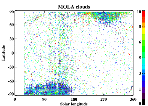
Figure 2: Cloud top altitude (km) from MOLA observations binned in  1°x1° latitude-solar longitude grid.

Figure 3: Zonal mean CO₂ mass mixing ratio in the northern polar region as a function of altitude, averaged between L_s = 180° to 360°.

Figure 4: Same as Fig. 3, except for the south pole during L_s = 0° to 180°.

Conclusion

The microphysical module for CO₂ clouds of LATMOS coupled with the Martian Global Climate Model of the Institut Pierre Simon Laplace has reproduced qualitatively the CO₂ ice clouds in winter polar regions in the first full-year simulations. Further analysis needs to be done to complete the study of these CO₂ ice clouds and compare more quantitatively to the observational data. We will also study more in detail the formation of mesospheric clouds in the martian atmosphere in the near future.

Acknowledgments

We thank our funders, the Agence National de la Recherche (project MECCOM, ANR-18-CE31-0013), the Laboratoire d'Excellence ESEP, and the French space agency CNES.

How to cite: Mathé, C., Määttänen, A., Audouard, J., Listowski, C., Millour, E., Forget, F., Spiga, A., Bardet, D., Teinturier, L., Falletti, L., Vals, M., Gonzàlez-Galindo, F., and Montmessin, F.: Global 3D modelling of Martian CO2 clouds, Europlanet Science Congress 2020, online, 21 Sep–9 Oct 2020, EPSC2020-751, https://doi.org/10.5194/epsc2020-751, 2020.

    Modeling clouds is a challenge we are currently facing in the development of Mars climate models. In particular, CO₂ clouds are exotic components of the Mars’ atmosphere that may imply rethinking some microphysical theories. Moreover, available datasets that could allow a better understand of involved processes are rare and, thus, must be analysed the best we can to acquire more information. The Mars Orbiter Laser Altimeter (MOLA, Smith and al., 1999) was an instrument aboard the Mars Global Surveyor spacecraft for a mission around Mars between 1997 and 2006 (MOLA provided data until 2001). MOLA’s first goal was to study Mars’s topography using laser altimetry in order to draw a precise map. However, range measurements have been made with a better precision than expected, allowing detection of features that were not assignable to the planet surface. Those features include clouds, especially polar winter CO₂ ice clouds that MOLA has been the first to detect. Previous studies conducted in the early 2000s (Neumann and al. (2003), Ivanov & Muhlemann (2001)) demonstrated that among all the laser returns, some were clearly clouds signatures coming from the atmosphere. However, the huge amount of data limited the manual analysis and forced the use of very strict distinction criteria, eventually leading to some misses.

    Our goal is to distinguish different categories of laser returns in MOLA data. A good modern option to computionally analyse MOLA data could be clustering methods, and K-means clustering methods in particular (Ackerman & Ben-David (2009)). For numerical reasons, we proceed to a first pruning to reduce the amount of data, assuming cloud returns could not be too close to the surface, by a typical range of less than ten meters from the MOLA vertical resolution (Abshire and al. (2010)) . We first apply the method on a single data file (that represents about 10 % of total data) then enlarge to the whole data set. We have led preliminary studies through empirical tests in order to define the best observational parameters for clustering among all those available in the raw data, best parameters being those allowing us to separate surface, noise and clouds returns. K-means methods are efficient ways of clustering but they require providing a predetermined number of clusters. That’s why we used three totally independent optimisation methods. Elbow method computes the total intra-cluster variation through total within-cluster sum of squares. Average silhouette method analyses clusters through « silhouette » score from distance of each point to its cluster and to closest one. Finally, gap statistic method (Tibshirani and al. (2001)) determines how far our clustering structure is from a random uniform distribution of points. All of these methods give us an « optimised » number of clusters to work with. The idea in this study is to find one cluster that would be a « cloud » cluster, containing all the non-surface non-noise laser returns. We plot geographical and temporal distribution of the different clusters separately in a first step, then more specifically for the wanted cloud cluster to verify the reliabily by comparison with previous studies. We can then work within the cloud cluster itself with clustering methods, to eventually find different types of cloud (and possibly dust).

    Following the reference paper for cloud detection in MOLA data (Neumann and al., 2003), the product of surface reflectivity and two-way transmissivity of the atmosphere, rT², appears as the best parameter for distinguishing cloud and surface returns, through the product of each laser return itself but also the average product of previous and next returns. Working on our test case (10 % of the data), our three independent optimisation methods converge to the same number of clusters. Among the clusters, cloud cluster is the one with both low rT² product and low average neighbors rT² (making a well-like shape in the time/rT² figure). Plotting the clusters shows that one of them identifies clouds returns. Another cluster could represent clouds boundaries or thinner clouds, while the other ones identify noise (low rT² product but high average neighbors product) and surface returns (high rT² product and high average neighbors product). We then move on to the whole data by applying our clustering method to each data file (around 10 % of data each time), plotting clusters for every file to eventually adjust the necessary number of clusters. Geographic and temporal plots of our cloud returns are in agreement with previous studies, presenting similar distributions. However, it seems like our method allows to find more clouds due to less stringent detection criteria. So far, we have not been able to find parameters to clearly separate the different type of clouds but a lot of possibilities are still to be tested.

    Because absorptive clouds can not really be attributed to a precise altitude, some of them may have been eliminated through our first pruning. It would be interesting to be able to cluster directly the whole data set but this requires some optimisation of our program. Moreover, evolution of the equipement capacities during the mission leads to different rT² continuum depending on the orbit : working with a normalised rT² product instead of raw rT² product itself should also be tested. Finally, if K-means methods are not adapted to work within the cloud cluster to distinguish reflective and absorptive clouds for example, it will be necessary to find another clustering method for the second step of our study. However, our results are promising and will hopefully help in complementing the first MOLA cloud climatology (Neumann and al. (2003)). Such observations are very important for comparing with microphysical model results ans helping us understand cloud formation process on Mars.

Acknowlegdements :

We thank the Agence National de la Recherche for funding (projet MECCOM, ANR-18-CE31-0013).

How to cite: Caillé, V., Määttänen, A., Spiga, A., Falleti, L., and Neumann, G. A.: Unsupervised Machine Learning Algorithms to Detect CO2 Clouds on Mars, Europlanet Science Congress 2020, online, 21 Sep–9 Oct 2020, EPSC2020-758, https://doi.org/10.5194/epsc2020-758, 2020.