MITM8

A self-organizing Kohonen map is a special type of artificial neural network. The neurons are arranged in a rectangular grid, so each neuron can be identified by two indices i and j. Besides its indices, each neuron carries a float vector. The network learns these vectors from randomly presented sample values. It evolves into a topologically correct two-dimensional map of the input data set.

The network is initialized with small random values for each neuron. It is then optimized by repeatedly iterating through the following steps:

• Randomly choose a vector r from the input data set.
• Find the neuron (i,j) whose vector r_i,j is closest to r in Euclidean distance r_i,j−r.
• Move the vector r_i,j towards r some fraction γ, γ≤1, of the distance, so the new value becomes

  r′i,j = ri,j + γ ( r − ri,j ) .     (1)

• Also move the vectors r_k,l of neurons (k,l) in the vicinity of (i,j) towards r, but weighted with a factor that decreases with the distance from (i,j), where the distance d is measured on the two dimensional map, i. e.,

  d = ((k−i)2+(l−j)2)1/2.     (2)

  With a Gaussian for the weighting factors, the updated vectors become

  r′k,l = rk,l + γ  exp(−d2/σ2)  ( r − rk,l )     (3)

  with some reach σ.

Step 4 ensures the formation of a topologically correct map. The parameters γ and σ have slowly to be turned down to zero towards the end of the optimization, the former to prevent noise introduced by the randomly selected input data, the latter to avoid excessive smoothing.

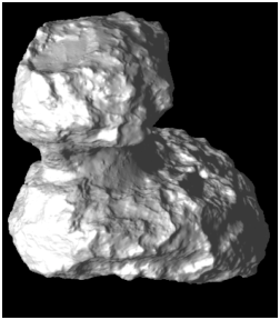
One application of such a self-optimizing Kohonen map is the mapping of the surface of a three-dimensional shape, like comet 67P/Churyumov-Gerasimenko, see Fig. 1.

 

Figure 1: Shape model of comet 67P/Churyumov-Gerasimenko.

 

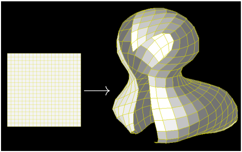
As input data, we use the three-dimensional positions of shape model vertices. The result of fitting a low resolution toy model to 67P is shown in Fig. 2.

 

Figure 2: Fitting a toy model of 21×21 neurons to the shape of comet 67P. This is just for illustration. The real map has much higher resolution.

 

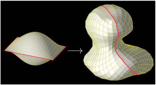
The map tries to sample the surface of the shape as evenly as possible. As a consequence, there is a gap between the edges of the map where they fold towards each other. The gap narrows with increasing resolution, however, by fitting a closed surface, see Fig. 3 we can avoid the gap at all. Moreover, the resultant map inherits the tessellation properties of the topologically equivalent Peirce quincuncial projection.

 

Figure 3: We construct a closed surface from two square grids of neurons connected at all four edges. This neural network learns the shape in the same way as the classical Kohonen map, however, it covers the complete surface without any gap. Again the real map has much higher resolution as this toy model.

 

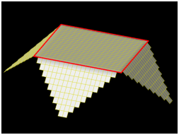
The resultant map is a shape model of 67P in its own right, albeit with relatively low resolution (the full scale model has 160,000 plates). But this shape model has the very special property that it can be unfolded to a two dimensional map. The are different possibilities how the closed structure is cut open and unfolded. One is illustrated in Fig. 4.

 

Figure 4: Unfolding of the closed surface into a two dimensional square map in quincuncial layout, which resembles the Peirce quincuncial projection of the world.

 

In this way, we obtain the Quincuncial Adaptive Closed Kohonen (QuACK) map of comet 67P.

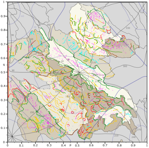
Any features on the surface of comet 67P can be projected onto the QuACK map. While the QuACK map has limited resolution (although much higher than the toy model illustrations shown here), features can be mapped with subgrid accuracy employing bilinear interpolation. An example of a geological QuACK map is shown in Fig. 5.

 

Figure 5: Example geological map of 67P in the QuACK map projection, from Leon-Dasi, M., S. Besse, B. Grieger and M. Küppers (2021).

 

How to cite: Grieger, B., Besse, S., Leon-Dasi, M., and Küppers, M.: QuACK: Quincuncial Adaptive Closed Kohonen maps for ducks and other odd shapes, Europlanet Science Congress 2021, online, 13–24 Sep 2021, EPSC2021-127, https://doi.org/10.5194/epsc2021-127, 2021.

We explore the performance of neural networks in automatically classifying asteroids into their taxonomic spectral classes. We particularly focus on what the methodology could offer the ESA Gaia mission. We constructed an asteroid dataset that can be limited to simulating Gaia samples. The samples were fed into a custom-designed neural network that learns how to predict the samples’ spectral classes and produces the success rate of the predictions. The performance of the neural network is also evaluated using three real preliminary Gaia asteroid spectra.

The overall results show that the neural network can identify taxonomic classes of asteroids in a robust manner. The success in classification is evaluated for spectra from the nominal 0.45–2.45 µm wavelength range used in the Bus-DeMeo taxonomy, and from a limited range of 0.45–1.05 µm following the joint wavelength range of Gaia observations and the Bus-DeMeo taxonomic system. The obtained results indicate that using neural networks to execute automated classification is an appealing solution for maintaining asteroid taxonomies, especially as the size of the available datasets grows larger with missions like Gaia.

How to cite: Penttilä, A., Hietala, H., and Muinonen, K.: Asteroid taxonomy using neural networks, Europlanet Science Congress 2021, online, 13–24 Sep 2021, EPSC2021-658, https://doi.org/10.5194/epsc2021-658, 2021.

Introduction
The knowledge of asteroid mineral composition is of high importance in planetary science, planetary defense, and in-space resource utilization. So far, mainly quantitative information on asteroid composition is derived by currently-used methods based on ratio of spectral parameters (band depths, band areas, band positions) or on spectral unmixing. These methods are highly sensitive to quality and consistency of input spectral data. In our approach we aim to test of using artificial neural networks (ANNs) for (semi-)quantitative mineralogical analysis of asteroid spectra.

Methods
Artificial neural networks have been developed to solve tasks which are difficult to define by exact mathematical methods and are less sensitive to quality of input data (in our case variation in spectral slope or absolute reflectance values). They are composed of layers of neurons. Each neuron of a layer is non-linearly connected with neurons in the following layer. The non-linearity makes the neural network flexible and enables it to solve various tasks. Neural networks consist of an input layer, any number of hidden layers, and an output layer. We utilize a neural network for determining modal and chemical compositions on the most common minerals presented in meteorites, i.e. olivine, orthopyroxene, clinopyroxene, and plagioclase. We implemented a so-called feed-forward neural network with one hidden layer . The inputs of the neural network are reflectances at different wavelengths. The outputs are modal composition of the observed sample and its chemical composition.

Data
We used measured reflectances from the Relab databse (http://www.planetary.brown.edu/relabdata/). We selected reflectance spektra of olivine and pyroxene which cover the wavelength interval between 350 nm and 2550 nm with a maximum step of 15 nm. These spectra were interpolated into a regular grid with a step of 5 nm. The interpolated spectra represent our input layer.

Results
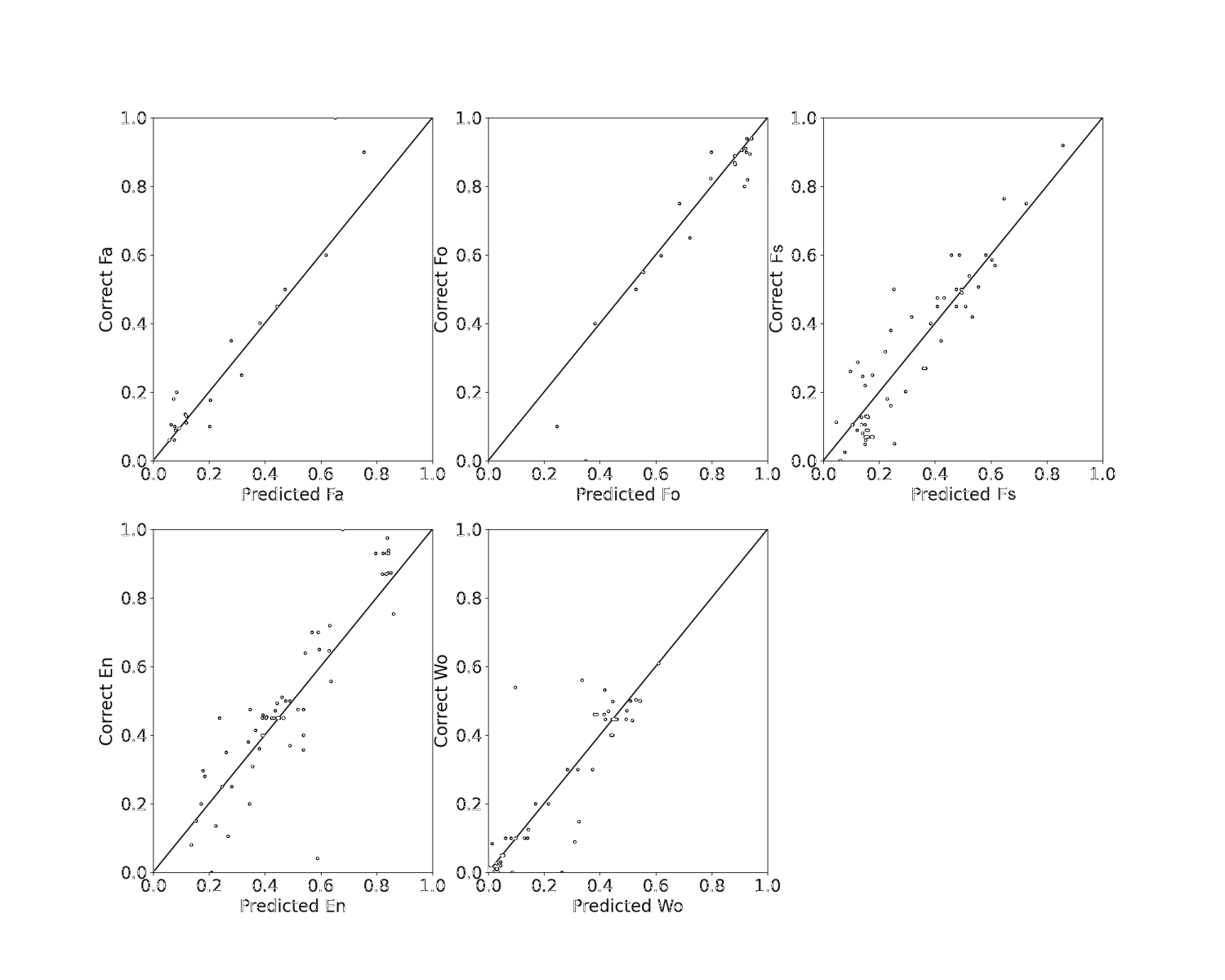
We applied the neural network on a set of olivine and orthopyroxene spectra. For this setup, we used 30 neurons in the hidden layer and 7 output layers (two for volume percentage of olivine and pyroxene, two and three for description of chemical composition of olivine and pyroxene, respectively). We split the data into two parts and used one of the parts for training the neural network. The results were evaluated on the other part. The results are shown in Fig. 1. The vertical axes show the correct (published) values while the horizontal axes the values predicted by the neural network.

Figure 1: Results of chemical abundances of olivines (top left and top middle panels) and pyroxenes
(other panels).

Discussion
Except a few outliers, the predicted values are within about 10% from the correct values. The outliers might be caused either by limited number of training samples or ambiguously determined “correct” values. However, the preliminary results are promising. In the near future, the prediction power of our neural network will be improved with more optimized architecture and increasing number of training samples.

How to cite: Korda, D., Kohout, T., Penttilä, A., and Klami, A.: Neural network for processing of asteroid spectra, Europlanet Science Congress 2021, online, 13–24 Sep 2021, EPSC2021-767, https://doi.org/10.5194/epsc2021-767, 2021.

The Moon Trek portal (https://trek.nasa.gov/moon) aims to provide the scientific community as well as the general public access to lunar data collected from various lunar missions. The portal also offers a suite of tools with the goal of allowing users to analyze the data for the purposes of education, mission planning, and research. Such tools include elevation profilers, crater and rock detection, lighting analysis, and slope analysis to name a few. Moon Trek is further expanding its analytic capabilities by adding feature detection to its toolset.

The feature detector, similar to the rock and crater detection tools, seeks to detect features on the lunar surface using orbital imagery. Unlike the detection tools currently available on the Moon Trek, the feature detector is built to be generic, trainable, and able to seek out any feature when provided a training set for the feature in question. The tool currently supports detection of craters, rocks, and lunar pits.

The feature detector takes a deep learning approach in finding features from orbital imagery. The model used in the latest detection tool is a Faster Region Based Convolutional Neural Network (Faster-RCNN) with a finetuning approach. More succinctly, the finetuning approach uses a model which has been developed and trained on a different and larger training set. The classification layer is replaced to detect features of the chosen domain (rocks, pits, craters, etc.) The model is then trained with smaller training sets.

Currently we use panchromatic Narrow Angle Camera (NAC) images from the Lunar Reconnaissance Orbiter Camera (LROC) as input. However, the model can be trained on orbital imagery from any mission. The tool’s output includes the NAC image with bounding boxes over detected and an ascii file showing pixel coordinates of each detected feature.

How to cite: Law, E., Gallegos, N., Nainan, C., and Malhotra, S.: Feature Detector on the Moon Trek Portal, Europlanet Science Congress 2021, online, 13–24 Sep 2021, EPSC2021-151, https://doi.org/10.5194/epsc2021-151, 2021.

Introduction

Mantle convection is a key driver of the long-term thermal evolution of terrestrial planets. Caused by the buoyancy-driven creeping flow of silicate rocks, mantle convection can be quantified through equations of conservation of mass, momentum and energy. These non-linear partial differential equations are solved through fluid dynamics codes such as GAIA [1]. However, the key parameters to these equations are poorly constrained. While the input parameters to the simulations are unknown, the outputs can sometimes be observed directly or indirectly using geophysical and geochemical data obtained via planetary space missions. Hence, the “observables” can be used to constrain parameters governing mantle convection. 

Given the computational cost of running each forward model in 2D or 3D (on the scale of hours to days), it is often impractical to run several thousands of simulations to determine which parameters can satisfy a set of given observational constraints. Traditionally, scaling laws have been used as a low-fidelity alternative to overcome this computational bottleneck. However, they are limited in the amount of physics they can capture and only predict mean quantities such as surface heat flux and mantle temperature instead of spatio-temporally resolved flows. Using a dataset of 2D mantle convection simulations for a Mars-like planet, [2] showed that feedforward neural networks are capable of taking five key input parameters and predicting the entire 1D temperature profile of the mantle at any given time during the 4.5-Gyr-long evolution of the planet.  Using the same dataset of forward models run on a quarter-cylindrical grid, we show that deep learning can be used to reliably predict the entire 2D temperature field at any point in the evolution. 

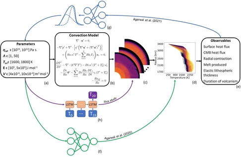
Fig. 1: Machine learning methods have been shown to work well for these low-dimensional observables such as the 1D temperature profile or components derived from it such as surface heat flux or elastic lithospheric thickness, both - (f) in a forward study ([2]) and (g) an inverse study ([3]). In this work, we demonstrate that (h) a surrogate can model 2D mantle convection using deep learning. 

Setup of mantle convection simulations

The mantle is modeled as a viscous fluid with infinite Prandtl number and Newtonian rheology under the extended Boussinesq approximation. The thermal expansivity and thermal conductivity are pressure- and temperature-dependent. Same applies to the viscosity, which is calculated using the Arrhenius law for diffusion creep. The bulk abundances of radiogenic elements are modified via a crustal enrichment factor, assuming that a crust of a fixed thickness formed very early in the evolution. Partial melting depletes heat-producing elements in the mantle and affects the energy balance. Finally, we add two phase-transitions in the olivine system. For a detailed description of the methods used, we refer to [2] and the references therein.

Compression of temperature fields

Each temperature field is of the size 302 x 394 grid points, making it a difficult task to predict such a high dimensional field from a limited amount of data. Hence, we first use convolutional autoencoders to compress each temperature field by a factor of 140 to a latent space representation, which is easier to predict (Fig. 2). 

Fig. 2: Convolutional autoencoders are used to compress the temperature fields by a factor of 140 to a so-called “latent space”. When constructed back to the original size, one can compute the difference between the original and the reconstructed field and use it to optimize the network weights.

Prediction of compressed temperature fields

As in [2], we test feedforward neural networks (FNN) to predict the compressed temperature fields from five input parameters plus time. We found that while the mean accuracy of the predictions relative to GAIA temperature fields was high (99.30%), FNN was unable to capture the sharper downwelling structures and their advection. The FNN fails to capture the rich temporal dynamics of convecting plumes and downwellings as the network only sees disconnected snapshots from different simulations (Fig. 3, upper panels).

To address this, we tested long short-term memory networks (LSTM), which have recently been shown to work in a variety of fluid dynamics problems (e.g. [4]). In comparison to the FNN, LSTM achieved a slightly lower mean relative accuracy, but captured the spatio-temporal dynamics much more accurately. The LSTM not only captures the downwellings, but also their advection in time (Fig. 3, lower panels). 

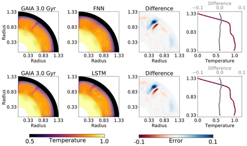
Fig. 3: Predictions from FNN (row 1) vs. LSTM (row 2), when compared with an  original GAIA simulation (column 1) in the test-set. Column 3 shows the difference between predicted and original temperature field, while column 4 shows the horizontally-averaged 1D temperature profiles from GAIA (solid blue) and from the machine learning algorithm (dashed red) as well as the difference between the two (grey line).

A proper orthogonal decomposition (POD) analysis (e.g. [5]) of the example simulation in the test-set shows that eigenfrequencies of the FNN predictions decay rapidly after only the first three to five modes. On the contrary, LSTM predictions are more energetic and hence, capture the flow dynamics more accurately (Fig. 4).

Fig. 4: Eigenfrequencies obtained through POD of the example simulation in the test-set.

References

1. C. Hüttig, N. Tosi, W. B. Moore, An improved formulation of the incompressible Navier–Stokes equations with variable viscosity, Physics of the Earth and Planetary Interiors, Volume 220, 2013, Pages 11-18, https://doi.org/10.1016/j.pepi.2013.04.002.

2. S. Agarwal, N. Tosi, D. Breuer, S. Padovan, P. Kessel, G. Montavon, A machine-learning-based surrogate model of Mars’ thermal evolution, Geophysical Journal International, Volume 222, Issue 3, September 2020, Pages 1656–1670, https://doi.org/10.1093/gji/ggaa234.

3. S. Agarwal, N. Tosi, P. Kessel, S. Padovan, D. Breuer, G. Montavon (2021). Toward constraining Mars' thermal evolution using machine learning. Earth and Space Science, 8, e2020EA001484. https://doi.org/10.1029/2020EA001484

4. Arvind T. Mohan, Dima Tretiak, Misha Chertkov & Daniel Livescu (2020). Spatio-temporal deep learning models of 3D turbulence with physics informed diagnostics, Journal of Turbulence, 21:9-10, 484-524. 10.1080/14685248.2020.1832230

5. L. Brunton and J. N. Kutz, 7 data-driven methods for reduced-order modeling, in Snapshot-Based Methods and Algorithms, edited by P. Benner, S. Grivet-Talocia, A. Quarteroni, G. Rozza, W. Schilders, and L. M. Silveira (De Gruyter, 2020)

How to cite: Agarwal, S., Tosi, N., Kessel, P., Breuer, D., and Montavon, G.: Deep learning for surrogate modelling of 2D mantle convection , Europlanet Science Congress 2021, online, 13–24 Sep 2021, EPSC2021-218, https://doi.org/10.5194/epsc2021-218, 2021.

Portable Fourier Ptychography Microscope (FPM) with Deep Learning Capability for Planetary Exploration

Thuc Phan¹, Thanh Nguyen^1,2, George Nehmetallah¹, and Shahid Aslam²

¹Catholic University of America, EECS, Washington DC, 20064, United States of America

²NASA, Goddard Space Flight Center, Greenbelt MD, 20771, United States of America

We present a portable FPM to perform wide field-of-view, high spatial-resolution imaging for biological samples. An NVIDIA Jetson-Nano board is used to computationally construct the images. The FPM has the potential to be compatible with space-based payloads [1].

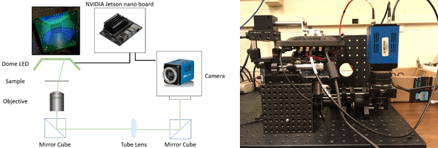
The compact FPM experimental system is shown in Fig. 1. The FPM is controlled by an NVIDA Jetson nano board with state-of-the-art machine learning processing capability. The camera captures low-resolution bright field and dark field intensity images corresponding to multiple illuminations of each light from the LED array. Different diffracted orders of light serve as the sub-complexed fields in the Fourier domain and are stitched under a constraint iterative process to perform the high-resolution reconstruction. The LED positions based on setup coordinates were digitally calibrated.

Figure 1. A portable inferencing FPM device. (left) Optical schematic, and (right) portable FPM tabletop setup. The NVIDIA Jetson Nano board enables the development of an inferencing deep learning pipeline to provide near real-time monitoring. The device is being tested by using a Lenovo Legion laptop and the following software packages: Python 3.8, Tensorflow/RT, CUDA 11.2, SPI-spidev, Open CV 4.0.

High-NA illuminators are needed for large space-bandwidth product imaging [2]. To achieve high-angle illumination with a sufficient signal-to-noise ratio in the darkfield region, the illuminators has a dome-like shape rather than planar shape [3]. A programmable dome array is made of five separate planar LED arrays that can illuminate up to 0.80 NA with discrete control of the RGB LEDs (Red: 625 nm, Green: 530 nm, and Blue: 485 nm) was used. The working distance is 65 mm. A 4x Nikon objective with 0.13 NA and a working distance of 17.2 mm was placed under the sample stage. This results in a larger synthetic NA of 0.93.

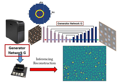
The device can be operated in a traditional FPM mode capturing intensity images and reconstructing 3D phase images with no deep learning (DL) capability (see Fig. 2). The normal mode is used to provide data for the DL mode to perform fresh training and testing. The DL model automatically detects if the sample is out-of-focus and then mechanically transits the sample to the focus plane using a translation stage or by digitally translating it into the focus position using DL. To implement near real-time monitoring, a DL model is used to speed up the DL-based FPM reconstruction by using 1 in 10 of the LED’s. This enhances the overall throughput of the system [4].

Figure 2. Deep learning framework for FPM inferencing. The generator network was trained under conditional generative architecture to predict the phase map. The trained generator model then was loaded on NVIDA Jetson Nano board to perform inferencing.

References

[1] Nguyen, T., et al. “Portable flow device using Fourier ptychography microscopy and deep learning for detection in biosignatures,” SPIE Defense and Commercial Sensing, Vol. 11401 (2020)

[2] Sun, J., et al. “Resolution-enhanced Fourier ptychographic microscopy based on high-numerical-aperture illuminations.” Sci. Rep. 7, 1187 (2017)

[3] Eckert, R., et al. “Efficient illumination angle self-calibration in Fourier ptychography.” Appl. Opt. 57, 5434-5442 (2018)

[4] Tian, L., et al. “Multiplexed coded illumination for Fourier Ptychography with an LED array microscope,” Biomed. Opt. Express 5, 2376-2389 (2014)

How to cite: Phan, T.: Portable Fourier Ptychography Microscope (FPM) with Deep Learning Capability for Planetary Exploration, Europlanet Science Congress 2021, online, 13–24 Sep 2021, EPSC2021-420, https://doi.org/10.5194/epsc2021-420, 2021.

Planetary magnetospheres create multiple sharp boundaries, such as the bow shock, where the solar wind plasma is decelerated and compressed, or the magnetopause, a transition between solar wind field and planetary field.
We attempt to use convolutional neural networks (CNNs) to identify magnetospheric boundaries, i.e.  planetary and interplanetary shocks crossings and magnetopause crossings in spacecraft in situ data. The boundaries are identified by a discontinuity in a magnetic field, plasma density, and in the spectrum of high-frequency waves. These measurements are available on many planetary missions. Data from Earth's missions Cluster and THEMIS are used for CNN training. We ultimately strive for successful classification of boundaries (shock, magnetopause, inbound, outbound) and the correct handling of multiple crossings.

How to cite: Ruedisser, H., Windisch, A., Amerstorfer, U. V., Píša, D., and Soucek, J.: Automatic Detection and Classification of Boundary Crossings in Spacecraft in situ Data, Europlanet Science Congress 2021, online, 13–24 Sep 2021, EPSC2021-226, https://doi.org/10.5194/epsc2021-226, 2021.