Europlanet Science Congress 2022
Palacio de Congresos de Granada, Spain
18 – 23 September 2022
Europlanet Science Congress 2022
Palacio de Congresos de Granada, Spain
18 September – 23 September 2022
MITM5
Machine Learning in Planetary Sciences

MITM5

Machine Learning in Planetary Sciences
Convener: Ute Amerstorfer | Co-conveners: Sahib Julka, Hannah Theresa Rüdisser, Mario D'Amore, Angelo Pio Rossi
Orals
| Thu, 22 Sep, 10:00–11:30 (CEST)|Room Andalucia 1
Posters
| Attendance Thu, 22 Sep, 18:45–20:15 (CEST) | Display Wed, 21 Sep, 14:00–Fri, 23 Sep, 16:00|Poster area Level 1

Session assets

Discussion on Slack

Orals: Thu, 22 Sep | Room Andalucia 1

Chairpersons: Ute Amerstorfer, Hannah Theresa Rüdisser
10:00–10:05
10:05–10:20
|
EPSC2022-480
Ingo Waldmann
The use of machine and deep learning is prevalent in many fields of science and industry and is now becoming more widespread in extrasolar planet and solar system sciences. Deep learning holds many potential advantages when it comes to modelling highly non-linear data, as well as speed improvements when compared to traditional analysis and modelling techniques.
One such problem is the identification and de-trending of stellar and systematic instrument noise in exoplanet lightcurves and in particular time-resolved spectroscopy of exoplanet atmospheres.
As part of the ESA Ariel Space mission and the European Conference on Machine Learning (ECML-PKDD), we have organised two very successful machine learning challenges in 2019 and 2021 (https://www.ariel-datachallenge.space).  The aim was to provide new solutions to traditionally intractable problems and to foster closer collaboration between the exoplanet and machine learning communities. Often interdisciplinary approaches to long-standing problems are thwarted by jargon and a lack of familiarity. Data challenges are an excellent way to break down existing barriers and establish new links and collaborations.
The top-ranked approaches range from deep-learning to gradient boosted extreme learning machines. In this presentation, I will discuss their pros and cons of solving the set challenge and show how new ideas generated by the data challenges can achieve real progress in the field.

How to cite: Waldmann, I.: The Ariel Machine Learning Data Challenge, Europlanet Science Congress 2022, Granada, Spain, 18–23 Sep 2022, EPSC2022-480, https://doi.org/10.5194/epsc2022-480, 2022.

10:20–10:30
|
EPSC2022-810
|
ECP
Adrian Kazakov, Anna Milillo, Francesco Lazzarotto, Stavro Ivanovski, Valeria Mangano, Miguel Escalona-Morán, Alessandro Mura, Stefano Massetti, Martina Moroni, Stefano Orsini, Roberto Sordini, Elisabetta De Angelis, Rosanna Rispoli, Alessandro Aronica, Nello Vertolli, Tommaso Alberti, Christina Plainaki, Fabrizio Nuccilli, and Raffaella Noschese

Abstract:

The exosphere of Mercury is the result of various processes and interactions of the surface with the planetary environment. The external factors acting on the planet, such as dust particles, solar wind protons and heavy ions, solar radiation and intense heat affect the composition and dynamics of the exosphere [1]. In turn, in situ exospheric measurements could allow us to derive surface information and complement surface mapping provided by devoted imagers, thus giving us additional information on the surface release processes, the dynamical interactions with the planetary environment, the erosion, space weathering and, eventually, about the evolution of the planet. At least two of the surface release processes - the micrometeorite vaporization and the ion sputtering - could serve as valid indicators of the regolith composition below, as they are stochiometric energetic surface release processes [2].

We hereby examine a tentative proxy method to derive the elemental and mineralogical composition of the regolith of Mercury from in situ measurements of its neutral exosphere through the use of deep neural networks (DNNs) [3]. We present a multivariate regression (MVR) supervised feed-forward DNN architecture whose inputs are the exospheric densities and proton precipitation fluxes measured in mock-up orbital runs through simulated Hermean exospheres [4] in view of the analysis of data from the SERENA (Search for Exospheric Refilling and Emitted Natural Abundances) instrument package on-board the Mercury Planetary Orbiter - part of the BepiColombo space mission to Mercury, nominal phase starting in 2026 [5]. The primary analysis task of the supervised learning algorithm is to predict from those exospheric measurements the constitution of the surface regolith below in terms of chemical elements and mineralogy. We show that, by learning from example, the DNNs can estimate the data generation mechanisms and allow us to omit the detailed analytical description of all the processes at the surface and in the exosphere, while at the same time give us a good approximation of the highly non-linear relationships between variables characterizing the release processes.

We further explore how the development of this method into nested DNNs could aid the constraining of the exopheric generation models and could give us even more insight into the interaction between the environment, the planetary surface and the exosphere. This way, we aim to add an artificial intelligence tool to our toolbox in the analysis of planetary data, which could be give us a new point of view on the exospheric measurements, thus breaking new ground for interpretations. [1] Milillo et al. 2005, SSR, 117, 397-443. [2] Killen et al. 2007, SSR, 132, (2–4): 433–509. [3] Kazakov et al. 2020, J. Phys.: Conf. Ser., 154, 12-14. [4] Mura 2005, PSS, 55, 1569–1583. [5] Orsini et al. 2020, SSR.

How to cite: Kazakov, A., Milillo, A., Lazzarotto, F., Ivanovski, S., Mangano, V., Escalona-Morán, M., Mura, A., Massetti, S., Moroni, M., Orsini, S., Sordini, R., De Angelis, E., Rispoli, R., Aronica, A., Vertolli, N., Alberti, T., Plainaki, C., Nuccilli, F., and Noschese, R.: Deep Neural Networks for Surface Composition Reconstruction from In Situ Exospheric Measurements at Mercury, Europlanet Science Congress 2022, Granada, Spain, 18–23 Sep 2022, EPSC2022-810, https://doi.org/10.5194/epsc2022-810, 2022.

10:30–10:40
|
EPSC2022-625
Jan-Peter Muller, Yu Tao, and Susan Conway

Introduction

High-resolution digital terrain models (DTMs) play an important role in studying the formation processes involved in generating a modern-day planetary surface such as the Moon. However, it has been a common understanding that DTMs derived from a particular imaging dataset can only achieve a lower, or at best, similar effective spatial resolution compared to the input images, due to the various approximations and/or filtering processes introduced by the photogrammetric and/or photoclinometric pipelines. With recent successes in deep learning techniques, it has now become feasible to generate pixel-scale topography using single-image DTM estimation (SDE) networks [1]. Although originally developed for Mars whose surface is very different due to the action of water and the distribution of dust through its perennially dusty thin atmosphere, the Moon has severe challenges due to the wide range of solar angles. Figure 1 shows an example of the 1 m/pixel LROC-NAC MADNet result produced using a 0.5 cm/pixel image compared with a 5m DTM generated using the standard Socet® photogrammetric process.

Figure 1. An example of 2 DTMs, the one of the left column generated at 5m using the SOCET® stereo photogrammetric processing chain at ASU whereas on the right column is the MADNet DTM generated at 1m.


Methods

Recent work on Mars on the MADNet 2.0 (multi-scale generative adversarial U-net based single-image DTM estimation) SDE system [ibid.] to produce single-input-image-based DTMs at twice the pixel-scale spatial resolution hads now been exploited to generate a 1m DTM of a large area on the lunar surface. Our study site is the von Karman crater located at 44.8°S 175.9°E on the lunar farside where the Chang’E-2 rover landed in November 2019 [2,3]. 370 LROC-NAC images were selected using ARCgis to minimise overlap and redundancy whilst trying to maintain the range of solar illumination angles. The coverage of these images is shown in Figure 2 superimposed on a coarse-scale (20m) DTM from Chang’E-2.

Figure 2. Coverage of 370 LROC-NAC ORI images in the resolution range of 0.5m-1.5m in their co-registered position to the Chang’E-2 14m MADNet DTM showing the dense coverage of the final DTM.

The different stages in the processing chain are shown schematically in Figure 3 emphasizing the different approaches between the photogrammetric stereo DTM pipeline and this new deep learning method, MADNet. With deep learning, we can simplify the complicated and time-consuming processes of the traditional stereo pre-processing, stereo matching, disparity refinement, interpolation and camera triangulation into one very fast image-to-height inference process, which only takes from a few seconds to a few minutes, given that the automated co-registration and multi-resolution height adjustment has been performed previously. Currently, this auto-coregistration process is the bottleneck although a COTS solution based on the Harris® ENVI® Modeler proved to be the most robust taking only a few minutes on a laptop. A specialist but low cost RTX3090 GPU is, however, required for the deep learning aspects.

Figure 3. Schematic flowchart of stereo photogrammetric process (upper panel) compared with this new deep learning based approach called MADNet.


Results

Co-registration and DTM height alignments were performed for the Chang’E-2 global 20m DTM using the SELENE+LOA global height reference map [4]. Training was performed using ≈400 pairs of ASU-PDS DTMs and images after careful screening to ensure only the highest possible quality were employed. Previous work on Mars indicates that a few bad training datasets would have catastrophic consequences on the MADNet prediction quality. In parallel 370 images were automatically co-registered to the 7m Chang’E-2 ORI mosaic using the proprietary ENVI® Modeler system. The results of the co-registration system are shown in Figure 2.

MADNet 2.0 is first applied to the 7m Chang’E-2 ORI image to produce a 14m DTM of the whole area. This is shown in Figure 4 using colour intensity height hill-shading for the CE2 mosaic and greyscale for the base reference of LOLA+SELENE over the base reference DTM.

Figure 4. MADNet applied to CE-2 (Chang’E-2) DTM to generate a 14m DTM superimposed on a 69m base DTM from SELENE+LOLA.


A preliminary analysis of the quality of the MADNet 14m CE-2 and LROC-NAC 1m DTM compared with a 5m ASU-PDS DTM is shown in Figure 5 This demonstrates the close congruence between all the 3 datasets as well as the fine-scale detail in the MADNet DTM compared with the other two datasets.

Figure 5. LROC-NAC 1m ORI superimposed on the 14m DTM where 4 profiles were extracted to show the high degree of agreement between the CE-2 (14m) , the 5m (PDS) and the 1m MADNet DTMs.


Conclusions

In this work, we have shown that we can apply MADNet SDE techniques to produce pixel-scale topography from Chang’E-2 mosaics and LROC-NAC images.

The final geotiff 1m DTM will be mosaiced and made available via the ESA Guest Storage Facility (GSF) at https://www.cosmos.esa.int/web/psa/ucl-mssl_meta-gsf as well as through the NASA Moontrek project (https://moontrek.jpl.nasa.gov). Given this capability large area maps using SDE could be produced for areas of interest to the NASA ARTEMIS project (which includes an ESA element) as well as ESA’s and China’s own lunar exploration plans.

Acknowledgements

The research leading to these results received initial funding from the UKSA Aurora programme (2018–2021) under grant ST/S001891/1, as well as partial funding from the STFC MSSL Consolidated Grant ST/K000977/1. The processing was supported by JPL contract no. 1668434. We thank Emily Law for all of her support for this work. S.C. is grateful to the French Space Agency CNES for supporting her GIS related work.

References

[1] Tao, Y.; Muller, J.-P.; Xiong, S.; Conway, S.J. MADNet 2.0. Remote Sens. 202113, 4220.

[2] Ren, X. et al. IEEE Trans. Geosci. Remote Sens. 2019,57, 6832–6843.

[3] Liu Z et al., Sci China Inf Sci, 2020, 63(4): 140901

[4] Barker, M. K. et al.. Icarus 273, 346–355 (2016).

How to cite: Muller, J.-P., Tao, Y., and Conway, S.: One metre 3D mapping of the Moon using the automated MADNet 2.0 single image height estimation, Europlanet Science Congress 2022, Granada, Spain, 18–23 Sep 2022, EPSC2022-625, https://doi.org/10.5194/epsc2022-625, 2022.

10:40–10:50
|
EPSC2022-473
Yu Tao, Jan-Peter Muller, and Susan Conway

Introduction
High-resolution digital terrain models (DTMs) play an important role in studying the formation processes involved in generating a modern-day planetary surface such as Mars. However, it has been a common understanding that DTMs derived from a particular imaging dataset can only achieve a lower, or at best, similar effective spatial resolution compared to the input images, due to the various approximations and/or filtering processes introduced by the photogrammetric and/or photoclinometric pipelines. With recent successes in deep learning techniques, it has now become feasible to improve the effective resolution of an image using super-resolution restoration (SRR) networks [1], retrieving pixel-scale topography using single-image DTM estimation (SDE) networks [2], and subsequently, combining the two techniques to produce subpixel-scale topography (Super-3D) from only a monocular-view input image [3]. 
Methods
Here we present our recent work [3] on combining the UCL (University College London) MARSGAN (multi-scale adaptive-weighted residual super-resolution generative adversarial network) SRR system [1] with the MADNet (multi-scale generative adversarial U-net based single-image DTM estimation) SDE system [2] to produce single-input-image-based DTMs at subpixel-scale spatial resolution [3]. Our study site is within the 3-sigma ellipse of the Rosalind Franklin ExoMars rover’s selected landing site (centred near 18.275°N, 335.368°E) at Oxia Planum.
We use the 4 m/pixel ESA Trace Gas Orbiter Colour and Stereo Surface Imaging System (CaSSIS) “PAN” band images and the 25 cm/pixel NASA Mars Reconnaissance Orbiter High Resolution Imaging Science Experiment (HiRISE) “RED” band images as the test datasets. We apply MARSGAN to the original CaSSIS and HiRISE images, and subsequently, we apply MADNet SDE to the resultant 1 m/pixel CaSSIS SRR images and the 6.25 cm/pixel HiRISE SRR images, to produce CaSSIS SRR-DTMs at 2 m/pixel and HiRISE SRR-DTMs at 12.5 cm/pixel, respectively. We show qualitative assessments for the resultant CaSSIS and HiRISE SRR-DTMs. We also provide quantitative assessments (refer to [3]) for the CaSSIS SRR-DTMs using the DTM evaluation technique that is described in [4].
Results
In this work, we perform qualitative assessment (visual inspections) for both the resultant 2 m/pixel CaSSIS SRR MADNet DTM mosaic and 12.5 cm/pixel HiRISE SRR MADNet DTMs. A small exemplar area (refer to “Zoom-in Area-1” in Figure 1 for its location) of the CaSSIS SRR MADNet DTM mosaic that overlaps with the HiRISE PDS DTM (DTEEC_039299_1985_047501_1985_L01), demonstrating the different level of details of the 25 cm/pixel HiRISE PDS ORI, the 1 m/pixel CaSSIS SRR image, the 4 m/pixel original CaSSIS PAN band image (MY34_004925_019_2_PAN), the shaded relief images of the 8 m/pixel CaSSIS MADNet DTM, 2 m/pixel CaSSIS SRR MADNet DTM, 1 m/pixel HiRISE PDS DTM, and the 50 cm/pixel HiRISE MADNet DTM, as shown in Figure 2.
 
Figure 1. Locations of the exemplar zoom-in areas are demonstrated next. Left: 25 cm/pixel HiRISE PDS ORI (ESP_039299_1985_RED_A_01_ORTHO) superimposed on top of the resultant 1 m/pixel CaSSIS SRR image mosaic [3], superimposed by the 1-sigma (red) and 3-sigma (dark-blue) ellipses of the Rosalind Franklin ExoMars rover’s planned landing site at Oxia Planum; Right: multi-level zoom-in views of the same HiRISE PDS ORI.

Figure 3 shows an example of Super-3D applied to CaSSIS imagery firstly in terms of SRR using MARSGAN and then using the SDE to produce this new Super-3D product.

 
Figure 2. Visual comparisons of a small exemplar area (i.e., “Zoom-in Area-1”) of the reference 25 cm/pixel HiRISE ORI, the resultant 1 m/pixel CaSSIS SRR image, the input 4 m/pixel CaSSIS PAN band image, shaded relief images of the resultant 8 m/pixel CaSSIS MADNet DTM, the resultant 2 m/pixel CaSSIS SRR MADNet DTM, the reference 1 m/pixel HiRISE PDS DTM, and the reference 50 cm/pixel HiRISE MADNet DTM (from top to bottom).
Conclusions
In this work, we show that we can use coupled MARSGAN SRR and MADNet SDE techniques to produce subpixel-scale topography from single-view CaSSIS and HiRISE images. The resultant CaSSIS and HiRISE SRR MADNet DTMs are published through the ESA Guest Storage Facility (GSF) at https://www.cosmos.esa.int/web/psa/ucl-mssl_meta-gsf. We recommend that readers download full-size full-resolution SRR and DTM results and look at their details. 
Acknowledgements
The research leading to these results is receiving funding from the UKSA Aurora programme (2018–2021) under grant ST/S001891/1. S.C. is grateful to the French Space Agency CNES for supporting her HiRISE related work. 

 
Figure 3. An example in the same region of Oxia Planum showing the original 4M CaSSIS image and the corresponding 1m MARSGAN SRR and the retrieved height models from the images shown above. 
References
[1] Tao Y et al. Remote Sens. 2021, 13, 1777. 
[2] Tao, Y. et al. MADNet 2.0:. Remote Sens. 2021, 13, 4220.
[3] Tao, Y. et al. Remote Sens. 2022, 14, 257.
[4] Kirk, R.L. et al. Remote Sens. 2021, 13, 3511.

How to cite: Tao, Y., Muller, J.-P., and Conway, S.: Super-3D: Subpixel-Scale Topography Retrieval of Mars Using Deep Learning, Europlanet Science Congress 2022, Granada, Spain, 18–23 Sep 2022, EPSC2022-473, https://doi.org/10.5194/epsc2022-473, 2022.

10:50–11:00
|
EPSC2022-842
Mars events detection with hybrid recurrent scattering neural network using InSight mission data
(withdrawn)
Grégory Sainton, Salma Barkaoui, Angel Bueno Rodriguez, Maartin de Hoop, Philippe Lognonné, Matthieu Plasman, Antoine Lucas, Taichi Kawamura, Keisuke Onodera, Aymeric Spiga, Alexander Stott, and Naomi Murdoch
11:00–11:10
|
EPSC2022-997
|
ECP
Daniel Le Corre, Nigel Mason, Jeronimo Bernard-Salas, David Mary, and Nick Cox

Recent technological advances have enabled satellites orbiting planetary bodies to retrieve more abundant streams of data faster. Machine Learning (ML) and other computer vision techniques provide the opportunity to analyse such data with higher accuracies and within shorter time-scales – much shorter than any human can achieve. However, the use of ML in planetary science is not accelerating at the same rate as in the related fields of geophysics or astronomy [1].

In this presentation we will present progress in creating ML tools for planetary surface feature detection. The goal of these tools is to fully exploit previously untapped volumes of available space data.

We will present an automated tool called the Martian Pit Shadow extractor (MAPS) which can detect the shadows cast by Martian pits and calculate their apparent depths. We will also present the results of applying MAPS to a current feature catalogue in the Mars Global Cave Candidate Catalog (MGC3) [2]. Pits are circular-to-elliptical depressions on the surface of terrestrial planets, which are most likely caused by gravitational collapse into a sub-surface void. These features are potential entrances to underground networks of evacuated lava tubes [3] and the depth of the pit is a factor that will influence the volume of the intact lava tube [4]. The propensity for ice caves to exist on Mars also increases with the thickness of the cavity’s ceiling [5], which itself will be larger for deeper pits. The purpose of MAPS is to automatically extract the shadow from a single cropped image of a Martian pit, as a means of calculating its apparent depth without the need for corresponding stereo images or elevation data. The apparent depth is defined as the depth of the pit at the extent of its shadow along the Sun’s line of sight [6]. MAPS has been tested with several methods of image segmentation with varying degrees of complexity from watershed transformation up to K-Means clustering. The next step is to adapt MAPS to other datasets to analyse pits on other planetary bodies such as the Moon.

Acknowledgements: This project has received funding from the European Union's Horizon 2020 research and innovation programme under grant agreement No 101004214.

[1] Azari, A.R.; Biersteker, J.B.; Dewey, R.M.; Doran, G.; Forsberg, E.J.; Harris, C.D.; Kerner, H.R.; Skinner, K.A.; Smith, A.W.; Amini, R.; Cambioni, S. Integrating machine learning for planetary science: Perspectives for the next decade, 2020, arXiv:2007.15129.

[2] Cushing, G.E. Mars Global Cave Candidate Catalog, PDS4 Archive Bundle, PDS Cartography and Imaging Sciences Node (IMG), 2015.

[3] Cushing, G.E.; Titus, T.N.; Wynne, J.J.; Christensen, P.R. THEMIS observes possible cave skylights on Mars, Geophysical Research Letters, 2007, 34, L17201, doi:10.1029/2007GL030709.

[4] Sauro, F.; Pozzobon, R.; Massironi, M.; De Berardinis, P.; Santagata, T.; De Waele, J. Lava tubes on Earth, Moon and Mars: A review on their size and morphology revealed by comparative planetology, Earth-Science Reviews, 2020, Vol. 209, 103288, ISSN 0012-8252, doi.org/10.1016/j.earscirev.2020.103288.

[5] Williams, K.E.; McKay, C.P.; Toon, O.B.; Head, J.W. Do ice caves exist on Mars? Icarus, 2010, Vol. 209, Issue 2, pp 358-368, ISSN 0019-1035, doi.org/10.1016/j.icarus.2010.03.039.

[6] Wyrick, D.; Ferrill, D.A.; Morris, A.P.; Colton, S.L.; Sims, D.W. Distribution, morphology, and origins of Martian pit crater chains, Journal of Geophysical Research, 2004, 109, E06005, doi:10.1029/2004JE002240.

How to cite: Le Corre, D., Mason, N., Bernard-Salas, J., Mary, D., and Cox, N.: Planetary Surface Feature Detection Using Machine Learning, Europlanet Science Congress 2022, Granada, Spain, 18–23 Sep 2022, EPSC2022-997, https://doi.org/10.5194/epsc2022-997, 2022.

11:10–11:20
|
EPSC2022-882
|
ECP
Small object detection network for monitoring mass wasting activity in the Martian North polar region
(withdrawn)
Oleksii Martynchuk, Lida Fanara, and Juergen Oberst
11:20–11:30
Display time: Wed, 21 Sep 14:00–Fri, 23 Sep 16:00

Posters: Thu, 22 Sep, 18:45–20:15 | Poster area Level 1

Chairperson: Ute Amerstorfer
L1.114
|
EPSC2022-47
|
ECP
Hannah Theresa Rüdisser, Andreas Windisch, Ute V. Amerstorfer, David Píša, and Jan Soucek

Planetary magnetospheres create multiple sharp boundaries, such as the bow shock, where the solar wind plasma is decelerated and compressed, or the magnetopause, a transition between solar wind field and planetary field.We attempt to use deep learning to identify magnetospheric boundaries, i.e. planetary and interplanetary shocks crossings and magnetopause crossings in spacecraft in situ data. The boundaries are identified by a discontinuity in a magnetic field, plasma density, and in the spectrum of high-frequency waves. These measurements are available on many planetary missions. Data from Earth's missions Cluster and THEMIS are used for training. We ultimately strive for successful classification of boundaries (shock, magnetopause, inbound, outbound) and the correct handling of multiple crossings.

How to cite: Rüdisser, H. T., Windisch, A., Amerstorfer, U. V., Píša, D., and Soucek, J.: Automatic Detection and Classification of Boundary Crossings in Spacecraft in situ Data, Europlanet Science Congress 2022, Granada, Spain, 18–23 Sep 2022, EPSC2022-47, https://doi.org/10.5194/epsc2022-47, 2022.

L1.115
|
EPSC2022-163
|
ECP
David Korda, Antti Penttila, Arto Klami, and Tomas Kohout

Introduction
Legacy methods which provide us with quantitative information on asteroid composition are based on spectral unmixing or specific spectral parameters (band depths, band areas, positions of band minima). These methods are sensitive to quality of input data and our apriori knowledge about the asteroid. We introduce a new approach based on artificial neural networks, which allows us to derive modal and chemical compositions of olivine-pyroxene-rich asteroids with precision better than 10 percentage points.

Data
We used measured reflectance spectra of olivine and pyroxene from the RELAB and C-tape databases. We selected spectra which were measured at least from 450 nm to 2450 nm with a resolution of 15 nm or better. Eventually, we interpolated these spectra to a wavelength grid with 5-nm spacing, denoised them using a convolutional filter, and normalised them at 550 nm. In total, we collected 510 reflectance spectra (100 olivine, 102 orthopyroxene, 108 clinopyroxene, 137 laboratory olivine-pyroxene mixtures, and 63 meteorites). For each spectrum, we have information about the sample modal abundances (in volume percent) and chemical composition (represented by end-members of individual mineral).
Model
An artificial neural network is a multi-parametric empirical model. Free parameters of the model are set (trained) according to input and output data. The neural networks are formed of layers of neurons. The basic layers are the input layer, the hidden layers, and the output layer. The layers are sequentially non-linearly connected. The non-linearity makes the neural-network model flexible enough to solve various tasks.

We trained a neural network for determining mineral modal abundances and mineral chemical compositions of olivine, orthopyroxene, and clinopyroxene, which are the major constituents of S-complex-like meteorites. The implemented neural network is made of an input layer, two convolutional hidden layers, and an output layer. The input layer inputs reflectance values at given wavelengths. The reflectance values are propagated through the model and result in the mineral modal abundances in volume percent and mineral chemical compositions represented by the mineral end-members.

Results
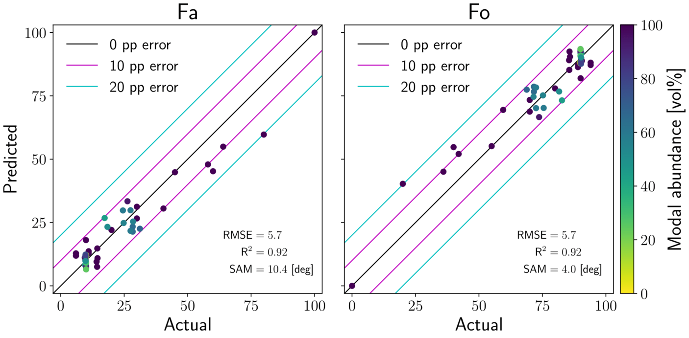
We evaluated accuracy of the trained model on different set of olivine, pyroxene, and olivine-pyroxene-mixture spectra. We found that modal abundances can be estimated with RMSE better than 10 percentage points, and chemistry of olivine and orthopyroxene with RMSE of about 5.7 percentage points. RMSE of clinopyroxene chemistry is about 11 percentage points. The results for olivine chemistry is shown in Fig.1. 

We applied the trained neural network on olivine-pyroxene-rich asteroid spectra (DeMeo et al., 2009; Binzel et al., 2019). We found a good agreement between S-type and Q-type asteroids and ordinary chondrites. Additionally, the model predicted that V-type asteroids are made of almost pure pyroxene, and A-type asteroids of almost pure olivine. The model revealed a systematic shift in olivine fraction between S-type and Q-type asteroids.

Discussion
We compared the neural-network predictions with the legacy band-area / band-centre-based methods (Cloutis et al., 1986; Gaffey et al. 2002; Reddy et al. 2015) and found that our predictions on modal abundances and chemistry are closer to the actual values and the validity region of our model is larger.

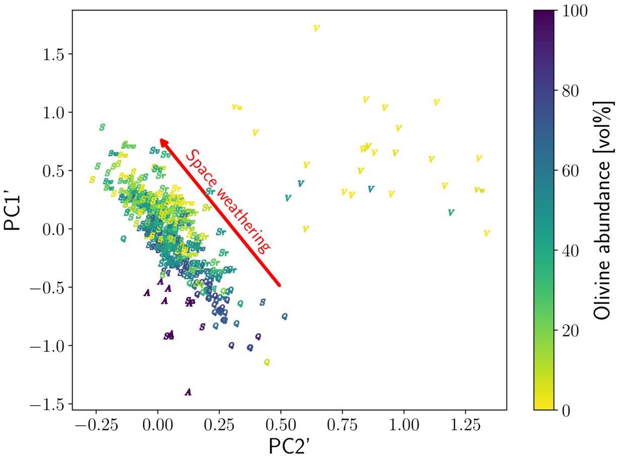
When analysing S-complex asteroid spectra, we observe apparent systematic depletion of olivine in S-type asteroids compared to Q-type asteroids, which have olivine abundance similar to those of ordinary chondrites. We hypothesise that this can be an effect of space weathering rather than compositional trend. Olivine undergoes space weathering changes in shorter timescale compared to pyroxene. Therefore, the space-weathering-attenuated absorption bands of olivine naturally results in relatively lower predicted olivine abundance compared to pyroxene.

We tested the hypothesis using (1) principal-component-based classification with determined space-weathering direction (Binzel et al., 2019), and using Chelyabinsk meteorite with (2) laboratory-induced space weathering and (3) its mixtures with spectrally featureless dark impact-melted or shock-darkened phases. The overall silicate mineralogical composition of Chelyabinsk meteorite in cases (2) and (3) remained consistent. In the PCA graph (1) in Fig. 2 and in weathered Chelyabinsk (2), we observed apparent depletion of olivine with increasing weathering, while the olivine abundance remained constant in the mixtures with darkened material (3). Even a large (50% and more) portion of spectrally neutral phase did not change predictions made by our model significantly. 


Conclusions
These results show that our model is sensitive to relative changes in strength of individual mineral absorptions, while at the same time is insensitive to wavelength-independent spectral attenuation. On weathered asteroids, the model is capable of finding locations which are fresher or more weathered if slowly varying modal abundance is assumed

References
Binzel, R. P., DeMeo, F. E., Turtelboom, E. V., et al. 2019, Icarus, 324, 41
Cloutis, E. A., Gaffey, M. J., Jackowski, T. L., & Reed, K. L. 1986, J. Geophys. Res., 91, 11, 641
DeMeo, F. E., Binzel, R. P., Slivan, S. M., & Bus, S. J. 2009, Icarus, 202, 160
Gaffey, M. J., Cloutis, E. A., Kelley, M. S., & Reed, K. L. 2002, in Asteroids III (University of Arizona Press, Tucson), 183–204
Reddy, V., Dunn, T. L., Thomas, C. A., Moskovitz, N. A., & Burbine, T. H. 2015, in Asteroids IV (University of Arizona Press, Tucson), 43–63

How to cite: Korda, D., Penttila, A., Klami, A., and Kohout, T.: Neural network for determining asteroid composition, Europlanet Science Congress 2022, Granada, Spain, 18–23 Sep 2022, EPSC2022-163, https://doi.org/10.5194/epsc2022-163, 2022.

L1.116
|
EPSC2022-680
|
ECP
Mireia Leon-Dasi, Sébastien Besse, and Alain Doressoundiram

Evidence of explosive volcanism on the surface of Mercury has been identified in the form of vents and pyroclastic deposits using images and spectral data acquired by the MESSENGER mission (Goudge et al. 2014, Thomas et al. 2014, Jozwiak et al. 2018, Pegg et al. 2021). Understanding the history of the volcanic eruptions forming these features provides an insight in the geological and thermal evolution of the planet. To this end, it is important to constrain the characteristics of each vent and, correlating them with the environment, classify the features according to their age and geological conditions. An individual analysis of a selection of vents has been carried out by Barraud et al. 2021 and Besse et al. 2015, providing new insights on the size, volcanic content and spectral properties of these features. However, performing a global analysis presents further challenges.  The collection of volcanic features identified presents a wide variety of characteristics in terms of morphology (simple vent, pit vent, vent-with-mound etc.), shape (circular, elliptical, curved), location (crater centre, crater rim, inter-crater plain), distribution (isolated or compound) and spectral properties of the pyroclastic deposit. This introduces a large number of variables that complicate the characterisation and timing of volcanic eruptions. 

The vast amount of data returned by the MESSENGER mission offers both a challenge and an opportunity in the methodology to solve this problem. While the combination of a large number of observations from different instruments can complicate the physical interpretation of a given process, it opens the door to the use of machine learning techniques. These methods rely on the identification of patterns on the input data without considering the associated physics, with the aim to reveal underlying correlations that can then be related to physical and chemical phenomena. This technique has been applied to the entire dataset collected by the Mercury Atmospheric and Surface Composition Spectrometer (MASCS), to classify the visible-near-infrared reflectance spectra into three categories (D'Amore et al. 2022). 

In this work, we investigate the application of machine learning to explore the differences amongst the pyroclastic deposits and volcanic vents, with the aim of improving the understanding on the evolution of explosive volcanism in Mercury. In this methodology we combine data from the MASCS and the Mercury Laser Altimeter (MLA) instruments with other properties of the vent surroundings (e.g., crustal thickness). By treating unrelated physical variables together as components of the same input vector, the outcome is a set of dimensions that have no direct physical meaning but can uncover underlying structures to be later physically or chemically interpreted. 

How to cite: Leon-Dasi, M., Besse, S., and Doressoundiram, A.: Exploring the diversity in pyroclastic deposits and volcanic vents on Mercury with machine learning techniques, Europlanet Science Congress 2022, Granada, Spain, 18–23 Sep 2022, EPSC2022-680, https://doi.org/10.5194/epsc2022-680, 2022.

L1.117
|
EPSC2022-1066
|
ECP
Nikolaj Dahmen, John Clinton, Men-Andrin Meier, Simon Stähler, Doyeon Kim, Alex Stott, and Domencio Giardini

InSight seismic data and marsquake catalogue

NASA's InSight seismometer has been recording the seismicity of Mars for over 3 years and to date, over 1300 seismic events were found by the Marsquake Service (MQS) [1,2]. Marsquakes usually have a low signal-to-noise ratio (SNR) and are consequently often hidden or contaminated by the background noise, making their detection and analysis challenging. Local winds interact with the lander and seismometer system and generate noise levels that fluctuate throughout the Martian day and regularly exceed typical event amplitudes. Additionally, extreme temperature changes cause transient high-amplitude spikes [3]. Conventional tools, such as the STA/LTA detectors, perform poorly on this dataset, as the various noise signals often share a common bandwidth and can be similar in duration to marsquakes [3]. Therefore, MQS detects events by manual data review and discriminates them from wind noise [4] by comparing the seismic data to onboard wind measurements if available, or otherwise, to the excitation of wind-driven lander modes. MQS classifies events by their frequency content into low- (<10%) and high-frequency (>90%) event families and assigns a quality based on their locatability (A: highest to D: lowest quality) [1].

Marsquake detection with convolutional neural network

Deep learning methods, and in particular convolutional neural networks (ConvNet) are nowadays routinely used for complex tasks such as speech or visual object recognition [5]. Here, we use a ConvNet architecture designed for image segmentation [6] to detect marsquake energy in the time-frequency domain. We train the ConvNet to predict segmentation masks that pixel-wise identify event and noise energy based on the time-frequency representation of a given waveform. We use the method to detect marsquakes and to decompose their signal in event and noise components. This allows us to estimate the marsquake duration, frequency content, and SNR.  We use the ConvNet to extend the MQS catalogue and further highlight its value in removing noise contamination from marsquakes [7]. Since the MQS catalogue is much smaller than typically labelled datasets used in deep learning [7], we create a training set with synthetic events with stochastic waveform modelling [8]. Synthetic events mimic the different MQS event types in terms of frequency content and duration and are combined with recorded InSight noise to include all types of noise.

Results

We run our ConvNet-based detector on the complete 20 samples-per-second dataset (over 900 Martian days) and compare our results to the careful manually curated MQS catalogue: we can detect all high-quality events and the majority of low-quality events - in addition to these, we find many additional low SNR events. We extend the catalogue by ~50% more events, of which the majority belongs to the high-frequency event family. An overview of the MQS events and our new detections is given in Figure 1. Similar to the MQS catalogue, we find many events in the quiet evening periods during the spring and summer of the Martian year 1 and 2, and further increase the number of events during the nights when noise levels are elevated. During the high noise periods (day time and winter), when noise amplitudes are orders of magnitudes above typical event amplitudes, we do not confidently detect events apart from a few that fall into short quieter periods. Our results suggest that the MQS catalogue is essentially complete for high SNR events and further support previous findings [9] on the seasonality of high-frequency events and their increased activity in Martian year 2 compared to year 1.


Figure 1: Overview of seismic noise, catalogued MQS events and new detections from ConvNet: the background of the main figure represents the broadband, vertical component seismic noise level (data gaps shown in white). The symbols indicate different event types belonging to the low frequency (LF, BB) or high frequency family (2.4, HF, VF), and colours indicate the qualities in the MQS catalogue; new detections found with our ConvNet detector are shown with their predicted event family type. The panel on the left side shows the cumulative event count using MQS events (blue) and MQS events and new detections (red). The event numbers are dominated by the high frequency events (corresponding to over 90% of events).

References:

[1] Clinton et al. (2021), 10.1016/j.pepi.2020.106595

[2] InSight Marsquake Service (2022), doi.org/10.12686/a16

[3] Ceylan et al. (2021), 10.1016/j.pepi.2020.106597

[4] Charalambous et al. (2021) 10.1029/2020JE006538

[5] LeCun et al. (2015), 10.1038/nature14539

[6] Ronneberger et al. (2015), 10.1007/978-3-319-24574-4_28

[7] Zhu et al. (2019), 10.1109/TGRS.2019.2926772

[8] Boore (2003), 10.1007/PL00012553 

[9] Knapmeyer et al. 10.1016/j.epsl.2021.117171

How to cite: Dahmen, N., Clinton, J., Meier, M.-A., Stähler, S., Kim, D., Stott, A., and Giardini, D.: A Deep Marsquake Catalogue, Europlanet Science Congress 2022, Granada, Spain, 18–23 Sep 2022, EPSC2022-1066, https://doi.org/10.5194/epsc2022-1066, 2022.