Oral presentations and abstracts
This session welcomes abstracts addressing all aspects of ice giant systems including (but not limited to) the internal structure of the ice giants, the composition, structure, and processes of and within ice giant atmospheres, and ice giant magnetospheres, satellites, and rings. We also welcome interdisciplinary talks that emphasise the cross-cutting themes of ice giant exploration, including the relationship to exoplanetary science and the connections to heliophysical studies. The session will comprise a combination of solicited and contributed oral and poster presentations on new, continuing, and future studies of the ice giant systems and the connection of the ice giants to our current understanding of planetary origins, both in our solar system and around other stars. We welcome papers that
• Address the current understanding of ice giant systems, including atmospheres, interiors, magnetospheres, rings, and satellites including Triton;
• Advance our understanding of the ice giant systems in preparation for future exploration, both remote sensing and in situ;
• Discuss what the ice giants can tell us about solar system formation and evolution leading to a better understanding of the current structure of the solar system and its habitable zone as well as extrasolar systems;
• Address outstanding science questions requiring future investigations including from spacecraft, remote sensing, theoretical, and laboratory work necessary to improve our knowledge of the ice giants and their relationship to the gas giants and the solar system;
• Present concepts for missions, instruments, and investigations to make appropriate and useful measurements of the ice giants and ice giant systems.
Session assets
Uranus and Neptune are the last unexplored planets of the Solar System. I show that they hold crucial keys to understand the atmospheric dynamics and structure of planets with hydrogen atmospheres. Their atmospheres are active and storms are believed to be fueled by methane condensation which is both extremely abundant and occurs at low optical depth. This means that mapping temperature and methane abundance as a function of position and depth will inform us on how convection organizes in an atmosphere with no surface and condensates that are heavier than the surrounding air, a general feature of gas giants. Using this information will be essential to constrain the interior structure of Uranus and Neptune themselves, but also of Jupiter, Saturn and numerous exoplanets with hydrogen atmospheres. Owing to the spatial and temporal variability of these atmospheres, an orbiter is required. A probe would provide a reference profile to lift ambiguities inherent to remote observations. It would also measure abundances of noble gases which can be used to reconstruct the history of planet formation in the Solar System. Finally, mapping the planets’ gravity and magnetic fields will be essential to constrain their global composition, structure and evolution.
How to cite: Guillot, T.: Uranus and Neptune are key to understand planets with hydrogen atmospheres, Europlanet Science Congress 2020, online, 21 Sep–9 Oct 2020, EPSC2020-514, https://doi.org/10.5194/epsc2020-514, 2020.
We aim at investigating whether the chemical composition of the outer region of the protosolar nebula can be consistent with current estimates of the elemental abundances in the ice giants. To do so, we use a self-consistent evolutionary disc and transport model to investigate the time and radial distributions of H2O, CO, N2, and H2S, i.e., the main O-, C-, N, and S-bearing volatiles in the outer disc. We show that it is impossible to accrete a mixture composed of gas and solids from the disc with a C/H ratio presenting enrichments comparable to the measurements (70 times protosolar). We also find that the C/N and C/S ratios measured in Uranus and Neptune are compatible with those acquired by building blocks agglomerated from grains and pebbles condensed in the vicinities of N2 and CO ice lines in the nebula. In contrast, the presence of protosolar C/N and C/S ratios in Uranus and Neptune would imply that their building blocks agglomerated from particles condensed at higher heliocentric distances. Our study demonstrates the importance of measuring the elemental abundances in the ice giant atmospheres, as they can be used to trace the planetary formation location and/or the chemical and physical conditions of the protosolar nebula.
How to cite: Mousis, O., Aguichine, A., Helled, R., Irwin, P., and Lunine, J. I.: Ice lines and the formation of Uranus and Neptune, Europlanet Science Congress 2020, online, 21 Sep–9 Oct 2020, EPSC2020-613, https://doi.org/10.5194/epsc2020-613, 2020.
Neptune’s atmosphere is highly dynamic with atmospheric systems observable as bands and discrete cloud systems that evolve in time scales of days, weeks and years. Most of them are observed as tropospheric clouds and elevated hazes that appear highly contrasted in observations obtained in hydrogen and methane absorption bands in the red and near-infrared spectrum of the planet. Given the small size of Neptune as observed from Earth (2.3 arcsec), it is difficult to characterize most of these clouds. Basic questions such as if they are convective storms, vortices or clouds detached from atmospheric waves or bands can be difficult for an specific feature in a given observation [1]. Only Adaptive Optics or lucky-imaging instruments in 8-m telescopes or larger, and HST, can provide suitable data, but the difficulty to access enough observational time in these facilities suggests that a combination of data from several observing programs can help. Smaller telescopes can also play an important role since they can be used to follow the main cloud systems and cover the gaps between observations obtained by the larger telescopes. This can provide the life-time or drift rates of the largest meteorological systems allowing to compare observations of the same features observed months apart in the largest telescopes.
During the last few years we have combined observations obtained from a variety of telescopes to study the major cloud systems and understand their life-time and evolution [2, 3], including those of “companion” clouds linked to rare dark vortices that are only observable in blue wavelengths from space [2, 4, 5]. In this work we present our data for 2019 which consists of the following observations:
- HST observations from the Outer Planets Atmospheres Legacy program (OPAL).
- Several sets from Keck and Lick telescopes from different programs including some relatively frequent observations from the TWILIGHT program.
- GTC observations with the HiperCam instrument doing lucky-imaging.
- Calar Alto 2.2m telescope with the PlanetCam lucky-imaging instrument.
- One single observation from Gemini while testing an AO system.
- Additional observations from the Pic du Midi 1.05 m telescope.
- Images provided by amateur astronomers and available through the PVOL [6] database.
The combination of these data suggests more variability and less cloud activity in 2019 than in previous years with a lower number of features in the data sets obtained with smaller telescopes. We provide the identification of particular meteorological systems over late summer 2019 and present drift rates of different mid-latitude features in the south hemisphere that are close but separated enough to the Voyager zonal winds to deserve attention. Other cloud systems in the south polar region and north tropics seem to follow the Voyager wind profile.
Future punctual observations achievable with new observational facilities such as the JWST will benefit from the evolutionary time-lines of the major cloud systems of Neptune and their drift rates in the atmosphere provided by similar future campaigns.
References
[1] Hueso and Sánchez-Lavega, Atmospheric Dynamics and Vertical Structure of Uranus and Neptune's weather layers. Space Science Reviews, 2019.
[2] Hueso et al., Neptune long-lived atmospheric features in 2013-2015 from small (28-cm) to large (10-m) telescopes. Icarus, 2017.
[3] Molter et al., Analysis of Neptune's 2017 Bright Equatorial Storm, Icarus, 2019.
[4] Wong et al., A New Dark vortex on Neptune, The Astronomical Journal, 2018.
[5] Hsu et al., Lifetimes and Occurrence Rates of Dark Vortices on Neptune from 25 Years of Hubble Space Telescope Images, The Astronomical Journal, 2018.
[6] Hueso et al., The Planetary Virtual Observatory and Laboratory (PVOL) and its integration into the Virtual European Solar and Planetary Access (VESPA), Planetary Space Science, 2018.
How to cite: Hueso, R., de Pater, I., Chavez, E., Simon, A., Sromovsky, L., Sánchez-Lavega, A., Wong, M., Fry, P., Delcroix, M., Dhillon, V., Hernández-Bernal, J., Iñurrigarro, P., Littlefair, S., Marsh, T., Ordoñez-Etxeberria, I., Pérez-Hoyos, S., Redwing, E., Rojas, J. F., and Tollefson, J.: Monitoring Neptune's atmosphere with small and large telescopes: results for 2019, Europlanet Science Congress 2020, online, 21 Sep–9 Oct 2020, EPSC2020-354, https://doi.org/10.5194/epsc2020-354, 2020.
Uranus and Neptune have only been visited by one spacecraft, Voyager 2. Their atmospheres thus remain mysterious in terms of composition and dynamics, despite repeated efforts to observe them from the ground and earth-orbiting telescopes. Deep composition is key to constrain internal and formation processes but is difficult to measure with remote sensing techniques because of the condensation into various cloud layers of several key volatiles. Chemical complexification initiated by solar UV and magnetospheric electrons, as well as contamination by external sources (dust, comets, ring and satellite material), all occurring in the upper atmosphere but diffusing downward, can further complicate the situation because of the mixing of these various components caused by dynamics.
In this context, an atmospheric entry probe to measure key volatiles (e.g. noble gases, C, N, S, P) in the upper troposphere is highly desirable (Mousis et al. 2018, Cavalié et al. 2020) and would benefit from direct observational support from an orbiting spacecraft (Fletcher et al. 2020), as well as contextual ground-based supporting observations. All these measurements are essential to constrain the chemistry models we develop to better understand the composition and dynamics in the Ice Giant atmospheres. With a coherent set of models, ranging from 1D thermochemical and diffusion models for the tropospheres (Cavalié et al. 2017, Leconte et al. 2017, Venot et al. 2019, 2020) to 2D time-dependent photochemical models for the stratospheres and ionospheres (Hue et al. 2018, Dobrijevic et al. 2020), we aim at contributing to a better understanding of the Ice Giant composition and dynamics.
How to cite: Cavalié, T., Dobrijevic, M., Hue, V., and Leconte, J.: Chemistry and dynamics in the atmospheres of the Ice Giants: from the troposphere to the ionosphere, Europlanet Science Congress 2020, online, 21 Sep–9 Oct 2020, EPSC2020-53, https://doi.org/10.5194/epsc2020-53, 2020.
A number of images and analyses have demonstrated the presence of hazes and clouds in the atmosphere of the ice giants. While the formation of hazes is attributed to the methane dissociation in the high stratosphere by solar UV and energetic particles that leads to a number of chemical reactions (e.g. Moses et al., Icarus, 307, 2018), the observed clouds are the result of the condensation of CH4 and H2S in the troposphere (e.g. Irwin et al., Nature Astronomy, 2018). However, the lack of current limb observations taken at different tangent heights limits our knowledge about the vertical structure and optical properties of these aerosols. In this work, we will present different results obtained with a coupled cloud-haze microphysical model (Toledo et at., Icarus, 333, 2019; Toledo et at., Icarus, 350, 2020) used to constrain the particle size, density, vertical structure and time scale of aerosols in the ice giants. Our simulations show, among other results, high precipitation rates at pressures greater than 0.5 bar and timescales ranging from years (for the haze) to a few hours (CH4 clouds).
How to cite: Toledo, D., Irwin, P., Rannou, P., Fletcher, L., and Yela, M.: Constraints on aerosol structure and formation in the atmosphere of the ice giants from microphysics simulations, Europlanet Science Congress 2020, online, 21 Sep–9 Oct 2020, EPSC2020-593, https://doi.org/10.5194/epsc2020-593, 2020.
Many studies were carried out recently regarding the exploration of Ice Giants, in the context of the next NASA decadal survey in planetary sciences and astrobiology, of the next planning cycle in ESA's Science Programme, and of a possible NASA-ESA collaboration. A mission to an Ice Giant could include an atmospheric probe, to operate in the 1-10 bars pressure range. Its payload could comprise sensor(s) devoted to the measurement of electrical properties, plasma densities and conductivities.
In order to check the performances of such instruments, it is necessary to develop models of the electron and ion densities profiles, with and without aerosols, from which the electrical conductivities can be derived.
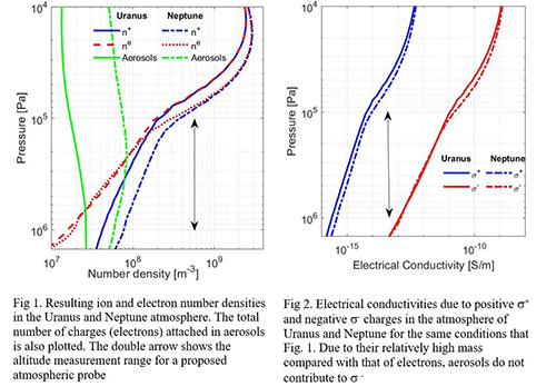
A model was developed based on studies performed at Mars and Titan [1-2], which computes the atmospheric positive and negative electrical conductivities between 0.1 and 15 bars in the atmosphere of Neptune and Uranus. In this altitude range, galactic cosmic rays ionize the atmospheric constituents, which react with atmospheric neutrals and aerosols, leading to the formation of ions heavier than the ones produced by cosmic rays. The densities of positive ions, electrons and charged aerosols are obtained by solving their corresponding continuity equations. It has been found that aerosol particles tend to be negatively charged due to the attachment of electrons, as a more efficient process than the attachment of positive ions. Therefore, the electrical conductivity due to negative charges is strongly reduced compared to the one expected when aerosols are not present. However, the electrical conductivity due to positive ions does not change so dramatically. The experimental determination of both components of the electrical conductivity can be useful to understand the properties of aerosols, plasma and electric currents in the atmospheres of Ice Giants.
Figure 1 and 2 shows some the first results of the number density and electrical conductivities in the atmospheres of Uranus and Neptune. They were calculated for a cosmic rays flux valid for a heliocentric potential of 100 MV, neglecting the planetary internal magnetic field, a mean ion mass of 100 amu and the aerosol particle distribution reported by Toledo et al. [3-4], which is extended down to the pressure range here considered.
References
[1] Cardnell, S., et al. (2016), A photochemical model of the dust-loaded ionosphere of Mars, J. Geophys. Res. Planets, 121, doi:10.1002/2016JE005077.
[2] Molina-Cuberos, G.J., et al. (2018) Aerosols: The key to understanding Titan's lower ionosphere, Planet. Space Sci, 153, 157 – 162, doi: 10.1016/j.pss.2018.02.007.
[3] Toledo et al. (2019), Constraints on Uranus's haze structure, formation and transport, Icarus 0019-1035, doi: 10.1016/j.icarus.2019.05.018
[4] Toledo et al. (2020) Constraints on Neptune’s haze structure and formation from VLT observations in the H-band, Icarus, doi: 10.1016/j.icarus.2020.113808
How to cite: Molina-Cuberos, G. J., Witasse, O., Montmessin, F., and Berthelier, J.-J.: Modelling of the Electrical Conductivities in the Atmosphere of Ice Giants, Europlanet Science Congress 2020, online, 21 Sep–9 Oct 2020, EPSC2020-523, https://doi.org/10.5194/epsc2020-523, 2020.
Context
One-dimensional modelling efforts for icy giant atmospheres have been performed in the past, from pioneering works to more recent comprehensive studies [2]. Circulation patterns in the troposphere and stratosphere inferred from visible, infrared, and microwave observations and models have been discussed in [3], but few fully three-dimensional models of Ice Giants have ever been presented.
Among the differences between these studies are the estimated radiative time constants and the consequences for the atmospheric circulation on Uranus and Neptune. For instance, comparing 2018 VLT images to Voyager data, Roman et al. [4] pointed out that the Uranian troposphere underwent almost no changes in terms of thermal structure over the intervening decades, pointing out that either the radiative time constants are much longer than estimated by Li et al. [2], or there is a very efficient energy redistribution by global circulation.
Deciphering such questions as well as preparing future observations require a supporting model able to adequately simulate atmospheric structure of these planets.
Method
Here, following what has been previously done for Saturn [5] and Jupiter [6], 1-D radiative-convective equilibrium modelling – corresponding to a GCM column in the absence of dynamics – is performed with a radiative-transfer code based on a correlated-k method and a two-stream solver. We utilise modern estimates of gaseous opacities, with vertical and horizontal distributions provided by photochemical modelling [7]. We explore the response to seasonal solar forcing along with the sensitivity to aerosols - with optical properties generated based upon Mie theory - which are poorly constrained by observations and therefore a source of uncertainties for radiative models.
Full 3-D simulations with dynamics are discussed in a companion abstract [8].
Results
First, aerosol-free simulations with planetary-averaged gaseous opacities lead to thermal structures that are globally too cold in the modelled stratospheres (e.g. more than 30K in the Uranian case). This ‘energy crisis’ in the middle atmosphere is an outcome that previous models have already been facing, and various processes have been proposed to solve the enigma, such as gravity waves breaking or radiative processes due to aerosols. Thus, in the present work, we investigate if and how this gap could be closed within our radiative model in the absence of dynamics, and provide some quantitative analysis of this ‘energy crisis’.
As photochemical models such as those by Moses et al. [7] point out, there exists considerable leeway in the choice of hydrocarbons profiles (e.g. assuming different eddy diffusion coefficients) to constrain our model that are still consistent with the available data. Furthermore, due to both seasonal photochemistry and atmospheric circulation, there are strong evidence for latitudinal variations of methane in both planets and some theoretical evidence for latitudinal variations of hydrocarbons, at least on Neptune. Hence we prescribe seasonal variations of their abundances within our radiative transfer based on KINETICS [7] outputs. On this basis, we present how the thermal structure and its seasonal patterns are affected.
In addition, we explore the parameter space of aerosol properties – within the range of observational constraints - with various sets of synthetic tropospheric clouds (CH4,H2S) and stratospheric haze (optical depth, albedo, particle size distribution, etc.).
For the different sets of simulations, we discuss the inferred radiative time constants, how they can be compared to previous work and how this will affect the circulation and constrain energy redistribution once dynamics is activated.
Finally, compared to previous works, we go one step further to provide a solid ground upon which the full 3-D circulation model for the Ice Giants can grow. Such work will be useful for interpreting future observations of Uranus and Neptune from the James Webb Space Telescope and new missions to these outer worlds.
Further reading
[1] Conrath et al., 1990 ; https://doi.org/10.1016/0019-1035(90)90068-K
[2] Li et al., 2018 ; https://arxiv.org/pdf/1806.02573.pdf
[3] Fletcher et al., 2020 ; https://arxiv.org/pdf/1907.02901.pdf
[4] Roman et al., 2020 ; https://arxiv.org/pdf/1911.12830.pdf
[5] Guerlet et al., 2014 ; https://doi.org/10.1016/j.icarus.2014.05.010
[6] Guerlet et al., 2019 : https://arxiv.org/pdf/1907.04556.pdf
[7] Moses et al., 2018 ; https://arxiv.org/pdf/1803.10338.pdf
[8] Milcareck et al., 2020, EPSC 2020 Abstract Book.
How to cite: Vatant d'Ollone, J., Fletcher, L. N., Guerlet, S., Roman, M. T., Moses, J., Milcareck, G., and Spiga, A.: Paving the way to an Ice Giants GCM : A radiative-convective modelling approach, Europlanet Science Congress 2020, online, 21 Sep–9 Oct 2020, EPSC2020-292, https://doi.org/10.5194/epsc2020-292, 2020.
Observations of Neptune, made in 2018 with the Multi Unit Spectroscopic Explorer (MUSE) instrument (in Narrow-Field Adaptive Optics mode) at the Very Large Telescope (VLT) and covering the wavelength range 480 – 930 nm were previously reported by Irwin et al. (Icarus, 311, 2019). Here, these observations have been reanalysed to incorporate more effectively the effects of limb-darkening following a new approach based on the Minnaert limb-darkening model, after Pérez-Hoyos et al. (Icarus, under review, 2020). The 800 – 900 nm region of our observations includes similar strength absorption bands of methane and H2–H2/H2–He collision-induced absorption, which allows changes in cloud-top altitude to be discriminated from methane abundance variations. Splitting the background atmosphere (i.e., away from bright, discrete clouds) into latitude bands, the measured variation of reflectivity with observed zenith angle at each wavelength is fitted with Minnaert limb-darkening coefficients, which can then be used to reconstruct the expected spectrum at any angle that can then be fitted with our retrieval model, NEMESIS (Irwin et al., JQSRT, 109, 2008). We find that this approach: 1) provides much stronger constraints on the cloud structure and methane abundance; 2) makes better use of all the available data and; 3) is more computationally efficient. We find a very similar variation in cloud-top (at ~3 bar) methane mole fraction as previously reported, but with much better characterized errors, and with mole fractions diminishing from ~5% at equatorial latitudes to ~3% in the south polar region. The retrieved latitudinal distribution of cloud-top methane abundance in Neptune's atmosphere can be seen in the figure below, where Neptune's south pole is at bottom left. We show that, although the reduction of methane abundance is well constrained (i.e., reducing by a factor 5/3 from the equator to the south pole), the absolute abundances are not so well determined. This is because the retrieved methane abundance also depends on the assumed background cloud properties, for which a number of different combinations are found to provide equally good fits to the data, but differ in their retrieved methane abundances by ±1%.
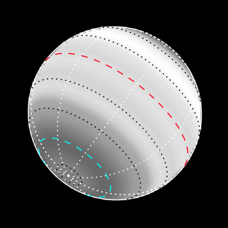
How to cite: Irwin, P., Dobinson, J., James, A., Toledo, D., Teanby, N., Fletcher, L., Orton, G., and Perez-Hoyos, S.: Limb-darkening reanalysis of latitudinal variation of cloud-top methane abundance in Neptune's atmosphere from VLT/MUSE-NFM, Europlanet Science Congress 2020, online, 21 Sep–9 Oct 2020, EPSC2020-241, https://doi.org/10.5194/epsc2020-241, 2020.
Introduction: NASA’s Spitzer Infrared Spectrometer (IRS) acquired mid-infrared (5-37 μm) disc-averaged spectra of Uranus very near its equinox over 21.7 hours on 16th to 17th of December 2007. A global-mean spectrum was constructed from observations of multiple longitudes, spaced equally around the planet, and have provided the opportunity for the most comprehensive globally averaged characterisation of Uranus’ temperature and composition ever obtained (Orton et al., 2014 a, b). In this work, we analyse the disc-averaged spectra at four separate longitudes to shed light on the discovery of longitudinal variability occurring in Uranus’ stratosphere during the 2007 equinox.
The composition and temperature structure of Uranus’ stratosphere is dominated by methane photolysis in the upper stratosphere (Moses et al., 2018). The complex hydrocarbons produced in these solar-driven reactions are the main trace gases present in the stratosphere and upper troposphere. These species are observable at mid-infrared wavelengths sensitive to altitudes between around one nanobar and two bars of pressure (Orton et al., 2014a).
Due to Uranus’ extremely high obliquity we can only clearly observe its longitudinal variation in disc-averaged observations close to its equinox. The northern spring equinox occurred in December 2007 with the aforementioned Spitzer observations occurring just 10 days after. The Spitzer data have been re-analysed using the most up to date pipeline available from NASA’s Spitzer Science Centre, resulting in minor changes over the previous reduction.
Longitudinal Variation: We assess the variations in discrete channels sensitive to different emission features. The radiances inside each interval are averaged and compared to the mean of all four longitudes. Each instrument module is exposed at a different time causing a spread of data points across the multiple longitudes displayed in Figure 1.
We detect a variability of up to 15% at stratospheric altitudes sensitive to the hydrocarbon species at around the 0.1-mbar pressure level. The tropospheric hydrogen-helium continuum and the monodeuterated methane that also arises from these deeper levels, both exhibit a negligible variation smaller than 2%, constraining the phenomenon to the stratosphere. Observations from Keck II NIRCII in December 2007 (Sromovsky et al., 2009; de Pater et al., 2011) and VLT/VISIR in 2009 (Roman et al. 2020) suggest possible links to these variations in the form of discrete meteorological features. In particular, Roman et al. (2020) identified discrete patches of brightness in 13-μm (acetylene) emission within a broad stratospheric band at mid-latitudes, which could be related to the variability observed by Spitzer.
Optimal Estimation Retrievals: Building on the forward-modelling analysis of the global average study, we present full optimal estimation inversions (using the NEMESIS retrieval algorithm, Irwin et al., 2008) of the low-resolution spectra at each longitude to distinguish between thermal and compositional variability. The model suggests that variations can be explained solely by changes in stratospheric temperatures. A temperature change of less than 2 K is needed to model the observed variation. This is compounded by results from high-resolution forward models (primarily sounding the ethane and acetylene emission) constructed using the parameters retrieved from the low-resolution spectra.
The data were best reproduced by models with atmospheric mixing via eddy diffusion that was weaker than that assumed by Orton et al. but still within the confines of a realistic fit according to their model. An eddy diffusion coefficient value of 1020 cm2sec-1 and a tropopause methane mole fraction of 8.0x10⁻⁵ provides the best fit to the temperature structure and the methane vertical profile whilst also maintaining the closest chi-squared value for the spectral fit (Moses et al., 2018).
Conclusion: The longitudinal variation detected at Uranus during the 2007 equinox is an observed physical change in the stratosphere of the planet, most likely a temperature change associated with the band of bright stratospheric emission observed in ground-based images. The Spitzer IRS data can provide much detail but without accompanying spatial resolution it is impossible to come to a definitive conclusion as to the origins of the changes.
The James Webb Space Telescope, when it launches in 2021, will provide much improved spectral and spatial resolution needed in the mid-infrared band to provide answers to the causes of the observed variation.
How to cite: Rowe-Gurney, N., Fletcher, L. N., Orton, G. S., Roman, M. T., Mainzer, A., Moses, J. I., de Pater, I., and Irwin, P. G. J.: Longitudinal Variations in the Stratosphere of Uranus from the Spitzer Infrared Spectrometer, Europlanet Science Congress 2020, online, 21 Sep–9 Oct 2020, EPSC2020-244, https://doi.org/10.5194/epsc2020-244, 2020.
In-situ probe measurements of planetary atmospheres add an immense value to remote sensing observations from orbiting spacecraft or telescopes, as highlighted and justified in numerous publications [1,2,3]. Certain key measurements such as the determination of noble gas abundances and isotope ratios can only be made in situ by atmospheric entry probes, but represent essential knowledge for investigating the formation history of the solar system as well as the formation and evolutionary processes of planetary atmospheres. Following the above rationale, a planetary entry mission to one of the outer planets (Saturn, Uranus and Neptune) has been identified as a mission of high priority by international space agencies. In the last Planetary Science Decadal Survey, a Uranus probe/orbiter was the highest priority for a future flagship Mission.
Within the scientific frame of atmospheric planetary sciences, a two- to three-year research study called IPED (Impact of the Probe Entry Zone on the Trajectory and Probe Design) investigates the impact of the interplanetary and approach trajectories on the feasible range of atmospheric entry sites as well as the probe design, considering Saturn, Uranus and Neptune as target bodies. The objective is to provide a decision matrix for entry site selection by comparing several mission scenarios for different science cases.
This talk introduces a tool development that focuses on the approach circumstances of a planetary entry probe upon arrival depending on science objectives of the entry sites. Science objectives are organised in four (planetocentric) latitude ranges: (1) low latitudes ‹15°, (2) mid latitudes between 15° and 45°, (3) high latitudes between 45° and 75° and (4) polar latitudes of ›75°. The latitude ranges are considered as potential entry zones for the IPED tool implementation. The final tool will allow mission designers and scientists to determine accessible entry sites (or regions) of a planet by using the hyperbolic entry velocity (direction, declination and absolute value) and the altitude of the entry interface point.
The IPED tool enables a 3D visualization of accessible / non-accessible latitudes depending on the range of selected parameters such as the flight path angle and the probe velocity at atmospheric entry, as well as environmental conditions of the destination planet such as the planet’s ring geometry and obliquity. The talk will present the status of work and first results, examples of which are displayed in the following figures for the planet Saturn for a case of a hyperbolic incoming velocity of v∞ = 12.06 km/s and an entry altitude of 700 km. Figure 1 shows the 3D overview of the planet’s system, with the black arrow representing the direction of approach asymptote of a probe trajectory aiming for the centre of gravity (flight path angle @ entry = 90°) and the shaded grey area being the ring structure of the planet. Variations of the B-plane vector and clock-angle result in a set of entry trajectories impact locations in the planet’s atmosphere are represented in dark green on the planet’s sphere. The trajectories are tested for safe ring crossing before impact (red points = unsafe, green points = safe). Unsafe trajectories are blocked and not considered in the evaluation. Figure 2 evaluates all entry points (dark green points in Figure 1) for specific characteristics at entry, mainly the flight path angle, the orbital and equal atmospheric relative velocity and the rotational speed of the planet at that latitude. The final development goal is a tool that allows a comparison of data based on different trajectories and approach asymptotes, launch windows and restrictions imposed by the probe design, such as limits on the flight path angle or entry velocity. The necessary development steps will be explained and discussed.
The presented research was supported by an appointment to the NASA Postdoctoral Program (NPP) at the Jet Propulsion Laboratory (JPL), California Institute of Technology, administered by Universities Space Research Association (USRA) under contract with National Aeronautics and Space Association (NASA). © 2020 All rights reserved.
[1] Mousis, O. et al., Scientific Rationale for Saturn’s in situ exploration, Planetary and Space Science 104 (2014) 29-47.
[2] Mousis, O. et al., Scientific Rationale for Uranus and Neptune in situ explorations, Planetary and Space Science 155 (2018) 12-40.
[3] Hofstadter, M. et al., Uranus and Neptune missions: A study in advance of the next planetary science decadal survey, Planetary and Space Science 177 (2019) 104680.
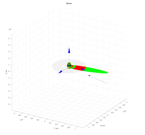
Figure 1 - 3D Overview on the evaluation space: The Saturn’s ring structure is displayed in grey, the body inertial reference frame as blue arrows, the asymptote of the incoming hyperbolic velocity as a black arrow, plane crossing trajectories in green (safe) and unsafe (red) and atmospheric entry locations in dark green.
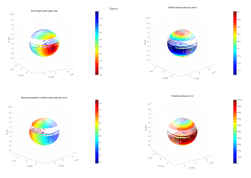
Figure 2 – Evaluation of all entry points (dark green points in Figure 1) for characteristics and their variation over the latitude / longitude at atmospheric entry at 700 km altitude: the flight path angle (upper left corner), the orbital velocity (upper right corner), equal atmospheric relative velocity (lower left corner) and the rotational speed of the planet (lower right corner).
How to cite: Probst, A., Spilker, L., Spilker, T., Atkinson, D., Mousis, O., Hofstadter, M., and Simon, A.: Assessing the Accessibility of different Latitudes for Planetary Entry Probe Missions to Saturn, Uranus and Neptune, Europlanet Science Congress 2020, online, 21 Sep–9 Oct 2020, EPSC2020-435, https://doi.org/10.5194/epsc2020-435, 2020.
The NASA Ice Giants Pre-Decadal Survey Mission Report (2017) recommended the high scientific importance of sending a mission with an orbiter and a probe to one of the Ice Giants, with preferential launch dates in the 2029-2034 timeframe. Such a mission concept is equally well supported by European scientists and Mousis et al (P&SS, 155, 12, 2018) give compelling scientific rationales for the exploration of these worlds with missions carrying in situ probes.
In this presentation we will outline the conceptual design of the Advanced Ice Giants Net Flux Radiometer (IG-NFR) instrument, currently being designed by NASA Goddard Space Flight Center to make in situ observations of the upward and downward fluxes of solar and thermal radiation in the atmospheres of Uranus and Neptune. The IG-NFR is designed to: (i) accommodate seven filter bandpass channels in the spectral range 0.25-300 µm (ii) measure up and down radiation flux in a clear unobstructed 10° FOV for each channel; (iii) use thermopile detectors that can measure a change of flux of at least 0.5 W/m2 per decade of pressure; (iv) view five distinct view angles (±80°, ±45°, and 0°); (v) predict the detector response with changing temperature environment; (vi) use application-specific integrated circuit technology for the thermopile detector readout; (vii) be able to integrate radiance for 2s or longer, and (vii) sample each view angle including calibration targets. The IG-NFR system noise equivalent power at 298 K is 73 pW in a 1 Hz electrical bandwidth.
We present initial simulations of the anticipated observations using two radiative transfer and retrieval tools, NEMESIS (Irwin et al., JQSRT, 109, 1136, 2008) and the Planetary Spectrum Generator (PSG, Villanueva et al., 2017, https://psg.gsfc.nasa.gov). For the NEMESIS modelling the radiative fluxes observable at varying pressure levels were calculated with a Matrix-Operator plane-parallel multiple-scattering model, using between 5 and 21 zenith angle quadrature points and up to 38 Fourier components for the azimuth decomposition. We also employed PSG to further validate our flux estimates, providing an important benchmarking and comparison test between both models. PSG solves the scattering radiative transfer employing the discrete ordinates method, with the scattering phase function described in terms of an expansion in terms of Legendre Polynomials. Molecular cross-sections are solved via the correlated-k method employing the latest HITRAN database (Gordon et al., 2017), which are completed with the latest collision-induced-absorption (CIA, Karman et al., 2019), and UV/optical cross-sections from the MPI database (Keller-Rudek et al., 2013). For the nominal case the Sun was assumed to be at an altitude of 10° above the horizon. The internal radiance field was calculated at each internal level for a standard reference Uranus atmosphere (e.g., Irwin et al., 2017) with the addition of a single cloud layer, based at 3 bar and composed of particles with a mean radius of 1.0 µm (and size variance 0.1) and assumed complex refractive index of 1.4 + 0.001i at all wavelengths. The opacity and fractional scale height of this cloud were fitted in both models to match the combined near-infrared observations of HST/WFC3, IRTF/SpeX and VLT/SINFONI analyzed by Irwin et al. (2017). The internal radiance fields were calculated from 0.4 to 300 µm using this atmospheric model.
We will show how these simulations are being used to guide the choice of spectral filter bandwidths and centres to optimize the scientific return of such an instrument. We will show that observations with such an instrument can be used to constrain effectively the radiation energy budget in the atmospheres of the Ice Giants and can also be used to determine the pressures of cloud and haze layers and broadly constrain particle size. Such modelling also allows us to simulate the visible appearance of Uranus’ atmosphere during a descent and to perform detailed validations of the simulations by comparing the two radiative transfer models (NEMESIS and PSG).
How to cite: Irwin, P., Calcutt, S., Dobinson, J., Alday, J., James, A., Roos-Serote, M., Aslam, S., Nixon, C., and Villanueva, G.: Modelling the expected observations of the Advanced Ice Giants Net Flux Radiometer (IG-NFR) instrument concept, under study for future entry probe missions to Uranus or Neptune., Europlanet Science Congress 2020, online, 21 Sep–9 Oct 2020, EPSC2020-306, https://doi.org/10.5194/epsc2020-306, 2020.
Above the dynamic clouds in Neptune’s atmosphere, the temperatures and photochemical composition within Neptune’s stratosphere are expected to respond to slowly modulating insolation over decades [1]. With Neptune’s seasons stretching over more than forty years, the entire history of reliable infrared observations resolving the planet’s disk comprises a mere fraction of a season. Yet, as we shall show, within this relatively brief window, observations appear to show changes in emission that would imply that sub-seasonal processes are significantly modifying the chemical and/or thermal structure in Neptune's stratosphere.
We present an analysis of the mid-infrared images and spectra of Neptune acquired using the VISIR instrument at the Very Large Telescope (VLT) between 2006 and 2018. Images in Q-band (17.65, 18.72, 19.50 µm) are used to infer upper-tropospheric temperatures (~200 mbar), while Neptune’s stratosphere (~1 mbar) is analyzed using a combination of imaging and spectra sensitive to emission from ethane (12.2 µm), methane (7.9 µm), and the S(1) hydrogen quadrupole (17.03 µm).
While we find that temperatures in the upper troposphere show no significant changes in time (remaining consistent with temperatures inferred from 1989 Voyager-IRIS measurements [2, 3]), the stratospheric emission appears to have changed unexpectedly over the past decade. Absolute radiances are uncertain, but relative trends in the spatially resolved emission are robust and show an asymmetric change in brightness temperature of up to ~3 K between and 2006 and 2008. The 2008 trend in emission continued throughout 2009 observations before returning to a relatively more symmetric pattern in 2018 (see Figure 1). Combined with the 2006 H2 S(1) quadrupole data, the observations indicate that the distribution of stratospheric emission observed in 2006 can likely be explained by the stratospheric temperature structure. However, no contemporaneous VLT-VISIR observations of the quadrupole emission were made in subsequent years, and so the nature of the observed changes between 2006 and 2008-2009 are ambiguous–they can potentially be explained by changes in the stratospheric temperatures, changes in the ethane abundances, or changes in both temperature and chemistry. The timing of these changes coincides with an extended maximum in Neptune’s photometric brightness following the 2005 southern summer solstice [4] and a decline in the discrete cloud coverage apparent in HST imaging [5]. Altogether, these observations suggest that Neptune’s stratosphere experiences intra-seasonal changes that may be coupled to dynamical forcing or variable mixing from the troposphere on timescales of years or less.
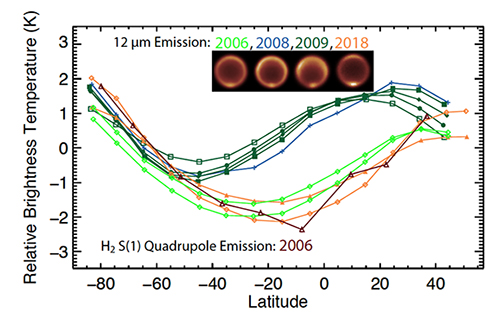
Figure 1. Relative variation in the longitudinally averaged brightness temperatures inferred from 12.2 µm emission (ethane at ~1 mbar) as a function of latitude for observations from 2006 (light green), 2008 (blue), 2009 (dark green) and 2018 (orange). Example images corresponding to these years are shown in the inset. Absolute calibrations are uncertain and show some spread, so relative trends have been normalized to roughly coincide (arbitrarily) at southern latitudes and the planet limbs, with zero here chosen by the mean. These trends show that the stratospheric emission in 2008 and 2009 differed in shape from those observed in 2006 and 2018, possibly indicating a change in stratospheric temperatures or ethane. The red curve shows the trend in stratospheric hydrogen quadrupole emission for 2006 and suggests that the observed trend in 12.2 µm emission in 2006 was likely primarily determined by the temperature structure.
[1] Moses, J. I., Fletcher, L. N., Greathouse, T. K., Orton, G. S., & Hue, V. 2018, Icar, 307, 124.
[2] Conrath, B.J., Flasar, F.M., Gierasch, P.J., 1991. Thermal structure and dynamics of Neptune’s atmosphere from Voyager measurements. J. Geophys. Res. 96, 18931–18939.
[3] Fletcher, Leigh N., et al. "Neptune at summer solstice: zonal mean temperatures from ground-based observations, 2003–2007." Icarus 231 (2014): 146-167.
[4] Lockwood, G. W. "Final compilation of photometry of Uranus and Neptune, 1972–2016." Icarus 324 (2019): 77-85.
[5] Karkoschka, Erich. "Neptune’s cloud and haze variations 1994–2008 from 500 HST–WFPC2 images." Icarus 215.2 (2011): 759-773.
How to cite: Roman, M. T., Fletcher, L. N., Orton, G. S., Vatant d'Ollone, J., Sinclair, J. A., Rowe-Gurney, N., Moses, J., and Irwin, P. G. J.: Sub-Seasonal Variations in Neptune's Stratospheric Infrared Emission from VLT-VISIR, 2006-2018, Europlanet Science Congress 2020, online, 21 Sep–9 Oct 2020, EPSC2020-471, https://doi.org/10.5194/epsc2020-471, 2020.
The dominant form of mass and energy transport between the Sun and the Ice Giant magnetospheres of Uranus and Neptune remains an open question. Predictions based on theory suggest that a combination of the weaker internal magnetospheric plasma sources and significantly tilted magnetic dipole fields of Uranus and Neptune may enable increased solar wind-magnetospheric coupling. Much of this coupling is dependent on the local solar wind parameters, specifically the Alfvénic Mach number (MA). Despite predictions of transport driven by solar wind coupling, the Voyager 2 flyby of Uranus observed a large MA of ~23 and a loop-like plasmoid in the magnetotail, suggestive of more internal planetary plasma driving. In order to better constrain the possible scenarios of internally-driven vs. externally-driven magnetospheric convection at a given planet, a quantitative assessment of upstream plasma variations is required. The interaction between the solar wind and a planetary magnetosphere is often parameterized in terms of MA, with lower values enabling enhanced rates of magnetopause reconnection and energy exchange between the interplanetary and planetary environments. Here we perform a comprehensive analysis of upstream MA throughout the solar system using data spanning from 0.3 AU to 75 AU, collected by the Helios 1 & 2, Voyager 1 & 2, and Pioneer 10 & 11 spacecraft from 1972-2005. We find that systematic increases in solar wind magnetic pressure during periods of high solar activity lead to lower-than-expected MA upstream of the giant planets. These lower MA values combined with the significant tilt of the magnetic dipole axes at Uranus and Neptune likely result in amplified solar-wind-magnetospheric coupling at solar maximum. The results indicate that magnetospheric dynamics at Uranus and Neptune may be strongly dependent on solar cycle.
How to cite: Gershman, D. and DiBraccio, G.: Solar cycle dependence of solar wind coupling at the Ice Giants, Europlanet Science Congress 2020, online, 21 Sep–9 Oct 2020, EPSC2020-258, https://doi.org/10.5194/epsc2020-258, 2020.
Abstract
Aurorae at the Gas Giants have been vital in understanding the magnetosphere-ionosphere coupling of these planets. The only aurorae we have detected at Uranus was in the ultraviolet spectrum from Voyager II in 1986 and in 2011 from Earth observations with the Hubble Space Telescope. Previous infrared observations at Uranus have shown promising evidence for infrared aurora but have been unable to confirm these sightings.
Using NIRSPEC observations over a single night in 2006, we aim to spatially resolve the infrared aurorae at Uranus. These are high spectral resolution observations revealing H3+ emission lines from pole-to-pole along the planet’s noon meridian, allowing us to measure H3+ brightness variations, temperature, and column density at all latitudes as a function of time. Our initial investigation shows local time peaks of H3+ emission intensities in the northern and southern half of observations, with no significant variations of ro-vibrational temperatures recorded. This strongly suggests that the H3+ brightness variation is driven by short timescale H3+ density variations, indicating these intensity peaks must occur due to other processes, such as the aurorae.
1. Introduction
Our understanding of the aurora of Uranus comes almost entirely from past ultraviolet observations of the planet, both from Voyager II’s flyby, which produced a complete mapping of these aurorae in the UV spectrum [1] and then, more recently, from the detections of bright auroral spots using the Hubble Space Telescope [2]. Since the first detection of H3+ at Uranus in 1992 [3], there has been a sustained effort to successfully detect the Uranian aurorae in the infrared. Due to the weak emission from Uranus [3] and limitations in spatial resolution (R < 2,500 [4]) of previous data, producing a map of Infrared emissions has posed a problem [5].
These past observations have either shown apparent enhancement in H3+ density from average emission across the entire disk of Uranus on individual observation nights [4], or have revealed localized brightening on the disk of the planet without resolving the temperature and H3+ density, thus not proving an auroral origin for the brightness enhancement [5] [6].
Using the Near InfraRed SPECtrometer on the Keck II telescope (R ~ 20,000), we have investigated a night of observations to detect local time variations in H3+ emissions and to measure the ro-vibrational temperatures, to determine the cause of these emissions, if auroral.
2. NIRSPEC Observations and Data Selection
Observations were taken between 07:26 and 13:23 UTC on 5th September 2006 with NIRSPEC on the Keck II Telescope. Using a 0.288x24” slit aligned to the planet’s N-S rotational axis, a total 224 spectro-images were analyzed. To mitigate the effects of sky emission in our data, we present a final 54 emission spectra sets. These contain five H3+ emission lines of the Q branch, between 3.9447 and 4.0042µm.
Measurements from Q(1,0-) and Q(3,0-) emission lines were taken due to their higher signal-to-noise ratio. By fitting the brightness (intensity) of both lines across all 54 datasets, local time variations can be measured. Due to a break (calibration star observations) and slit unalignment (between 10:52 and 11:31 UTC), data is left blank.
3. H3+ Emission Intensities
All 54 datasets were stacked horizontally with increasing time (Q(1,0-) emissions in Figure 1). Any vacant pixels correspond to anomalous data points.
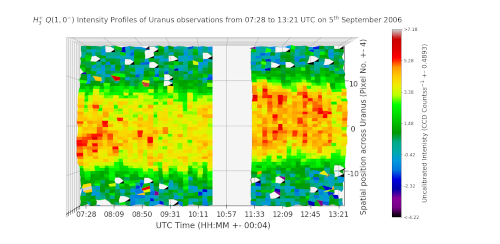
Figure 1: Local time variability of Q(1,0-) intensities across the slit. The pixel colour is dependent on intensity value, shown by the colour bar (right).
Between 07:28 and 08:15 UTC, we observe significant intensity peaks across Uranus (between 25% and 62% above local mean intensity). These peaks predominately occur in the negative spatial pixels where intensities are >20% greater than their positive counterparts. Between 11:27 and 13:03 UTC similar peaks of intensity are observed (between 12% and 49% above local mean intensity). In comparison, the intensities in the positive spatial pixels are >12% greater than the negative half but show no significant increase from earlier observations.
4. H3+ Ro-vibrational Temperatures

Figure 2: Temporal and spatial variability of H3+ temperature. The pixel colour is dependent on intensity value, shown by the colour bar (right).
Overall, a mean ro-vibrational temperature of 547K was measured between 07:28 and 08:15 UTC, 2% below the total mean temperature. A 1% increase in mean ro-vibrational temperature was observed between 11:27 and 13:03 UTC. We hence suggest that the ro-vibrational temperatures are not the cause of peak intensities in Figure 1.
5. Summary and Conclusions
Our initial findings show H3+ peaks between 07:28 to 08:15 UTC with further peaks observed between 11:27 and 13:03 UTC. These peaks appear independent to the ro-vibrational temperatures (which remains mostly constant). The latitudinal locations of these emissions across Uranus’s disk tied in with minimal thermal variation suggests that these emissions could be a result of the northern and southern aurorae of Uranus. If this is so, this makes our findings the first to spatially resolve Uranus’s infrared aurorae. Further work will involve column density measurements, with future work investigating ion velocities to understand ionospheric flows. Additionally, we will map this data across a 3D model of Uranus, to compare our findings with previous investigations of Uranus’s aurorae.
Acknowledgements
Emma Thomas was supported by an STFC studentship at the University of Leicester. All the data presented herein were obtained at the W.M. Keck Observatory, which is operated as a scientific partnership among the California and the National Aeronautics and Space Administration. The Observatory was made possible by the generous financial support of the W. M. Keck Foundation.
References
[1] Herbert, F. and Sandel, B.R., 1994. JGR Space Physics, 99(A3), pg. 4143-4160.
[2] Lamy, L., et al, 2012. Geophysical Research Letters, 39(7).
[3] Trafton, L.M., et al, 1993. The Astrophysical Journal, 524, pg. 1059-1083.
[4] Melin, H., et al, 2011. Astrophysical Journal, 729:134, pg. 9.
[5] Lam, H.A., et al, 1996. The Astrophysical Journal, 474, pg. 73-76.
[6] Melin, H. et al, 2019. Phil. Trans. R. Soc. A, 377: 20180408.
How to cite: Thomas, E., Stallard, T., Melin, H., and Chowdhury, N.: Searching for Uranus’s Infrared Aurorae from NIRSPEC Observations, Europlanet Science Congress 2020, online, 21 Sep–9 Oct 2020, EPSC2020-797, https://doi.org/10.5194/epsc2020-797, 2020.
All giant planets in the solar system have two types of moons as defined by their orbits and mode of origin. The first type, referred to as the regular moons, has tight circular orbits close to the equatorial plane of the host, implying primordial accretion in the circum-planetary disc. The second type, called the irregular moons, in contrast, is characterised by wide, highly-eccentric and -inclined orbits and are believed to be captured by their host from heliocentric orbits through some form of dissipation.
However, the Neptunian moon Triton, 3000 km across, does not neatly fit in any of the two categories — it is orbiting the host rather close-in but in a direction opposite to the spin of Neptune. The obvious incompatibility between its retrograde orbit and an in-situ accretion origin suggests that it was captured by Neptune, for example, as a component of a binary asteroid pair. Another moon in the system, Nereid, is a distant irregular satellite. It is the largest of its kind and at the same time features the tightest and the most eccentric orbit for an irregular moon.
Here we explore an in-situ formation formation for these two moons. We assume that both initially formed as regular satellites at Neptune. Then a planetary encounter triggers an evolutionary sequence of events for these two moons towards their observed orbits. Such an encounter cannot happen in the present solar system. But rather in the early solar system, there is an instability period as envisioned by the Nice scenario. Specifically in a later version of the Nice scenario where three gas giants (IG) are initially orbiting the Sun; during the instability period the additional IG gains a significant orbital eccentricity, allowing it to encounter other planets until finally ejected. Here, we model such an encounter between a moon-bearing Neptune and an IG.
We find that during the encounter, about half of the pre-existing Neptunian moons are ejected and the surviving moons are highly excited. Among the survivors, a few per cent gain retrograde orbits (Triton analogues, TAs) while a similar fraction acquire wide, eccentric orbit (Nereid analogues, NAs). While the NAs orbits match that of Nereid quite well, those of the TAs are highly eccentric. Often the orbit of the TA intersect that of the NA; then the latter will be removed due to scattering or collision within a Myr. How can the NA survive then? A further issue is after the Neptune-IG encounter, some of the other moons may also survive. Why are these additional moons not observed today?
We find that if these moons are small, collisions between them and the TA would eliminate the former without endangering the latter. Collisions also shrink the orbit of the TA, decouple from that of NA and hence NA is protected. Finally, tides takes control and circularise TA’s orbit on Gyr timescale.
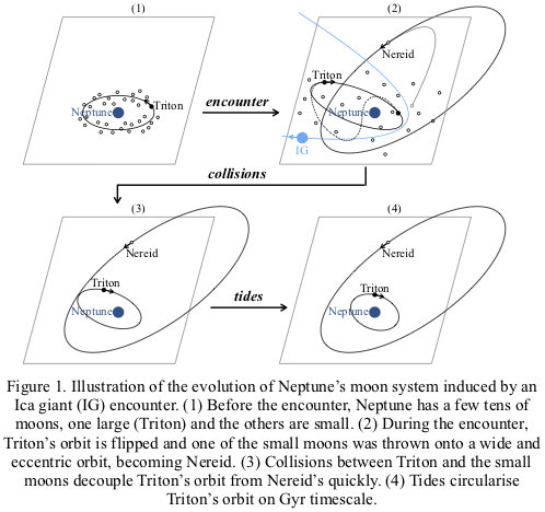
An illustration of our model is shown in Figure 1 and an example from the numerical simulations in Figure 2. Depending on how stringently we define a TA and NA, our model has an efficiency of 10^-5 - 10^-3.

In this in-situ formation model, Triton and Nereid accrete in the circum-planetary disk (see also, Harrington & Van Flandern, 1979, Icarus, 39, 131; Li et al. 2020, A&A, in press, doi: 10.1051/0004-6361/201936672) whereas the conventional capture model (e.g., Agnor & Hamilton, 2006, Nature, 441, 192; Nesvorny et al., 2007, AJ, 133, 1962) predicts that the two form in the circum-stellar disk. The environment, e.g., the temperature, in the two disks could be rather different, potentially leading to different compositional properties for example the fraction of volatiles. Hence, further observations as well as space missions would be helpful to constrain the formation path of the two moons.
Full details can be found in Li & Christou (2020, AJ, 159, 184).
The authors thank Dr. Craig B. Agnor for direct contributions to this work. DL acknowledges financial support from Knut and Alice Wallenberg Foundation (2014.0017 and 2012.0150) and from Vetenskapsrådet (2017-04945). The authors also thank the Royal Physiographic Society of Lund. Astronomical research at the Armagh Observatory and Planetarium is funded by the Northern Ireland Department for Communities (DfC).
How to cite: Li, D. and Christou, A.: An in-situ formation for Triton and Nereid, Europlanet Science Congress 2020, online, 21 Sep–9 Oct 2020, EPSC2020-769, https://doi.org/10.5194/epsc2020-769, 2020.
Introduction and Background
Trident is a mission concept to investigate Neptune’s large moon Triton, an exotic candidate ocean world at 30 AU (Prockter et al., 2019, Mitchell et al. 2019). The concept is responsive to recommendations of the recent NASA Roadmap to Ocean Worlds study (Hendrix et al., 2019), and to the 2013 Planetary Decadal Survey’s habitability and workings themes (Squyres et al., 2011).
The concept was chosen (Ref. 5) from proposals submitted in 2019, under NASA’s Discovery Program, and is currently in its Phase A, competing for selection with three other mission concepts.
Voyager 2 showed that Triton has active resurfacing with the potential for erupting plumes and an atmosphere. Coupled with an ionosphere that can create organic snow and the potential for a subsurface ocean, Triton is an exciting exploration target to understand how habitable worlds may develop in our Solar System and beyond. Using a single flyby, Trident would map Triton, characterize active processes and determine whether the predicted subsurface ocean exists.
Nominal mission
By launching during 2026, Trident would take advantage of a rare, efficient gravity-assist alignment, to capitalize on a narrow – but closing – observational window that enables assessment of changes in Triton’s plume activity and surface characteristics since Voyager 2’s encounter one Neptune-Triton season ago.
We have identified an optimized solution to enable a New Horizons-like fast flyby of Triton in 2038 that was proved to fit within the Discovery 2019 cost cap. The spacecraft has a robust design and uses high heritage instruments: (a) Infra-red spectrometer, (b) Narrow angle camera, (c) Wide-angle camera, (d) Triaxial magnetometer, (e) Radio science and (f) Plasma spectrometer. The mission concept builds on the New Horizons concepts of operation. Our overarching science goals are to determine: (1) if Triton has a subsurface ocean; (2) why Triton has the youngest surface of any icy world in the solar system, and which processes are responsible for this; and (3) why Triton’s ionosphere is so unusually intense.
Radio Science Instrument and Objectives
The Radio Science Instrument (RSI) is the assembly of the DST-R (Deep Space Transponder and Receiver) and USO (UltraStable Oscillator), see Fig. 1.
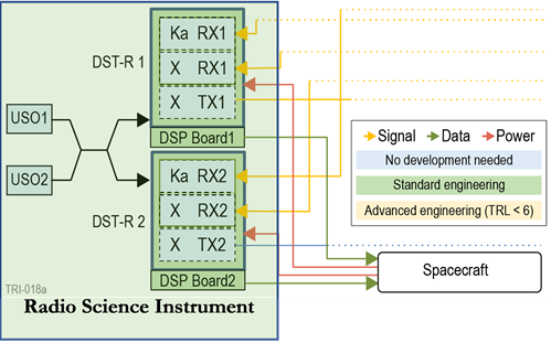
Fig. 1: Trident’s Block Diagram of the Radio Science Instrument
The RSI hardware involves no new technology or advanced development. The DST-Rs are provided by the Italian Space Agency (ASI). Dual USOs identical to the USO provided for the ESA/JUICE mission 3GM radio science experiment, are provided to ASI by the Israel Space Agency. ASI has a wide experience in providing RF instrumentation having led the development of several transponder units for deep space science missions in the last 30 years.
The USO feeds the DST-R and generates a stable frequency reference for the uplink radio signals to be recorded on board. The DST-R works at the same time as a phase-coherent Deep Space Transponder at X-band, but also as an on-board Receiver at X- and Ka-band.
The RSI contributes to two Trident science questions related to the science goals (1) and (3): “Is Triton an ocean world?” and “Why is Triton’s ionosphere so intense?”.
In particular, the RSI provides three physical parameters: (a) the electron density profiles on leading and trailing hemispheres, (b) temperature via neutral atmospheric density profile, and (c) the thickness of the hydrosphere from internal mass distribution. Physical parameters (a) and (b) are estimated through simultaneous, dual frequency (X-and Ka-band) uplink radio occultations while the physical parameter (c) is inferred by gravity science observations carried out via phase-coherent Doppler tracking at X-band.
Our quantitative requirements for the three above-mentioned objectives (a), (b) and (c) are as follows:
- measure the electron density in the ionosphere of Triton to +/- 10% of the population detected by Voyager, i.e. to a sensitivity of 4E+9 el/m3;
- measure the neutral atmosphere density and temperature to a sensitivity of +/- 0.1 Pa and +/- 5 K;
- measure the gravity quadrupole coefficient C22 with ≤10% error.
This paper shows how an optimal combination of on-board instrumentation, a careful trajectory design and an efficient radio science data processing strategy will lead to exceeding all quantitative radio science requirements listed above, with ample margins.
Acknowledgements
Authors PT, AB, LGC and MZ acknowledge financial support from Agenzia Spaziale Italiana (ASI), via contract No. 2020-13-HH.0 CUP F34I20000050005. This work was carried out in part at the California Institute of Technology, Jet Propulsion Laboratory under a contract from NASA. It describes a predecisional mission concept, for discussion and planning purposes only. The inputs of the various past and present members of the Trident team are gratefully acknowledged.
References
[1] L. M. Prockter, et al.: Exploring Triton with TRIDENT: a Discovery-Class Mission, 50th Lunar and Planetary Science Conference 2019 (LPI Contrib. No. 2132), Abstract 3188.
[2] K. L. Mitchell, et al.: Implementation of TRIDENT: a Discovery-Class Mission to Triton, 50th Lunar and Planetary Science Conference 2019 (LPI Contrib. No. 2132), Abstract 3200.
[3] Hendrix, A. R. et al. (2019) Astrobiology 19(1), doi:10.1089/ast.2018.1955.
[4] Squyres, S. W. et al. (2011) Vision and Voyagers for Planetary Science in the Decade 2013-2022, National Academies Press.
[5] https://www.nasa.gov/press-release/nasa-selects-four-possible-missions-to-study-the-secrets-of-the-solar-system
How to cite: Tortora, P., Oudrhiri, K., Bourgoin, A., Gomez Casajus, L. A., Zannoni, M., Buccino, D., Kaspi, Y., Galanti, E., Frazier, W., Prockter, L., Mitchell, K., and Howett, C.: TRIDENT Radio Science Objectives and Expected Performance, Europlanet Science Congress 2020, online, 21 Sep–9 Oct 2020, EPSC2020-1042, https://doi.org/10.5194/epsc2020-1042, 2020.
Marc Costa Sitjà1, Olivier Witasse2, Alfredo Escalante López1
1RHEA for European Sapce Agency,2European Space Agency
We present a systematic approach to analyse rapidly fly-by opportunities for the cruise phase of a mission to an Ice Giant. Such flyby would provide a unique opportunities to characterise Jupiter Trojans, Centaurs, or Jupiter Family comets.
A mission to an Ice Giant (Neptune and/or Uranus) will be among the ones examined by NASA's next Planetary Sciences and Astrobiology Decadal survey. ESA was exploring in 2018-2019 a potential collaboration to a NASA-led mission to an ice giant and has carried out a concurrent engineering design study [1] for possible European contributions. In this study, a dual launch in 2031 was contemplated; after a Jupiter swingby in late 2032, one orbiter would go to Uranus while the second one would reach Neptune.
The long cruise of a mission to Uranus and or Neptune would provide an excellent opportunity scientific investigations like heliophysics science [2], [3], [4]. In addition, it could provide an unexpected chance to visit an unexplored small body.
Examples of such flybys by missions to the outer solar system are well known. To mention some, the Rosetta spacecraft performed two flyb-bys of asteroid, 2867 Steins and 21 Lutetia [5]; Galileo performed fly-bys of 951 Gaspra and 243 Ida (these images provided the first direct confirmation of an asteroid moon, Dactyl) [6] and Cassini-Huygens performed a more humble fly-by of 2685 Masursky at about 0.011 AU.
In general flyby targets can only be chosen after launch from a list of candidates according to scientific interest, fly-by geometry, operational feasibility and the additional cost of propellant for the trajectory modifications [7]. The expected results from such observations include: the rotational properties of the target including the astrometric refinement of their orbit, the determination of their spin state and pole direction, global characteristics such as shape, volume, mass and bulk density, surface physical properties and morphology, detailed chemical and mineralogical characterization, effects of the space weathering on surface properties due to the solar wind interactions and exploration of the target's environment and activity.
We took a cruise trajectory to Neptune used in ESA's CDF study to search for a candidate flyby, as a check whether the science return of such mission could be enhanced. In this study, we checked whether a quick assessment of flyby opportunities for a candidate trajectory was possible.
In our analysis, we considered to search for JupiterTrojans, Centaurs, TransNeptunian Objects, and Jupiter-Family Comets [8]. The description provided for each family (sorted by orbit type) is the following:
For a preliminary assessment, we decided to use data from the JPL Small-Body Database Search Engine [9]. From the database we selected a total of 12507 bodies for which we retrieved the data in SPICE format (Spacecraft Kernel) [10]. To do so systematically, we used a Julia based client wrapper to Horizons [11] and then we took advantage of the SPICE Toolkit capabilities to perform a Closest Approach (CA) search for each body and obtain the time and distance of the event. We present preliminary results of our study hereby.
The results provide us with some interesting figures. The histogram below - table and in Figure 1- provides a wider view of the resulting distribution of objects as a function of the CA distance.
| Distance Bin (AU) | 0-0.1 | 0.1-0.5 | 0.5-1.0 | 1.0-2.0 | 2.0-100.0 |
| Number of objects | 1 | 7 | 12 | 42 | 12444 |
We selected some examples that are provided in the following table:
| Body Name | Family | Body ID | Inclination (deg) | CA (AU) |
| Shoemaker-Levy 9 | JFC | 1000183 |
5.982 |
0.16 |
| 335P/Gibbs | JFC | 1003007 | 7.27 | 0.07 |
| P/2015 TP200 | JFC | 1003474 | 8.77 | 0.38 |
| 2013 CT160 | C | 3667711 | 16.76 | 0.46 |
| 2019 TP13 | C | 3985102 | 4.93 | 0.44 |

The ongoing analysis shows that there is only one interesting result for the current trajectory: comet 335P/Gibbs. Such flyby could only be compared with the before mentioned Cassini 2685 Masursky at about 0.011 AU, in such case we would be seven times further and with such a rapid scenario we could already identify a potential flyby. Figure 2 shows a simulation of a theoretical Ice Giants flyby with 335P/Gibbs.
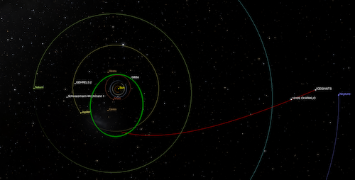
We repeat that this report is a very preliminary and approximate result, an updated will be given at the time of the conference. The main purpose of this contribution was to prove that such studies are feasible and can later help to optimise the trajectory design and the target selection process for fly-by opportunities. We plan to conduct such search with other mission such as JUICE and also to expand the catalogue of bodies for which we will conduct such searches.
[1] P. F. S. Bayon, Cdf study report: Ice giants (2019).
[2] L. N. Fletcher, Ice giant system exploration, white paper response to75esa call for voyage 2040 science themes (2019).
[3] C. Arridge, et. al., The science case for an orbital mission to uranus: Exploring the origins and evolution of ice giant planets, Planetary and Space Science 104 (2014) 122 – 140
[4] T. Bocanegra-Bahamon, et. al., Muse mission to the uranian system: Unveiling the evolution and formation85of ice giants, Advances in Space Research 55 (2015) 2190 – 2216
[5] M. Barucci, M. Fulchignoni, A. Rossi,Rosetta asteroid targets:892867 steins and 21 lutetia, Space Science Reviews 128 (2007) 67–78.
[6] M. J. Belton, C. R. Chapman, et.atl., Galileo’s encounter with 243 ida:An overview of94the imaging experiment, Icarus 120 (1996) 1 – 19
[7] F. B. T. Morley, Rosetta navigation for the fly-by of asteroid 2867 steins98(2009).
[8] B. Gladman, B. Marsden, C. Vanlaerhoven, Nomenclature in the outer solar system, The Solar System Beyond Neptune (2008)
[9] J. Giorgini, et.al., JP:’s on-line solar system data service
[10] C.H.Acton, Ancillary datas ervices of nasa's navigation and ancillary information facility, Planeary and Space Science 44 (1996) 65–70.
[11] J. A. Perez-Hernandez, An interface to nasa-jpl horizons system in julia
How to cite: Costa Sitjà, M., Witasse, O., and Escalante López, A.: Surveying potential cruise fly-by opportunities for an Ice Giant mission, Europlanet Science Congress 2020, online, 21 Sep–9 Oct 2020, EPSC2020-878, https://doi.org/10.5194/epsc2020-878, 2020.
Please decide on your access
Please use the buttons below to download the presentation materials or to visit the external website where the presentation is linked. Regarding the external link, please note that Copernicus Meetings cannot accept any liability for the content and the website you will visit.
Forward to presentation link
You are going to open an external link to the presentation as indicated by the authors. Copernicus Meetings cannot accept any liability for the content and the website you will visit.
We are sorry, but presentations are only available for users who registered for the conference. Thank you.