Oral presentations and abstracts

Introduction:  Estimates of asteroid (101955) Bennu’s gravity have been determined based on a series of independent solutions from different teams involved on the OSIRIS-REx mission. In addition to classical radio science techniques for estimating a body's gravity field coefficients, the discovery of particles ejected from Bennu that persist in orbit for multiple revolutions provides a unique opportunity to probe the gravity field to higher degree and order than possible by using conventional spacecraft tracking [1]. However, the non-gravitational forces acting on these particles must also be characterized, and their impact on solution accuracy must be assessed, requiring the different gravity field estimates to be compared and reconciled.

Given the measured gravity field of Bennu, rigorous constraints on its internal density heterogeneity can be found by comparing the measured field with the constant density field computed from the asteroid shape. These results in turn provide unique insight into the global geophysical processes that drive the external and internal morphology of small rubble-pile asteroids such as Bennu.

Finally, definitive results on the surface and close-proximity force environment of Bennu can be derived and updated from the initial analysis based on the total mass and constant density shape. Several aspects of the environment are highly sensitive to the gravity field and have changed from earlier results [2, 3, 4].

We will present the current gravity field solutions and uncertainties, update the surface and proximity environment models, and provide the geophysical implications and interpretations of these measurements.  

 Geophysical Models:  The estimated gravity field solutions are compared with the constant density shape model to constrain models of the internal density variation. We find that these differences are consistent with Bennu having an under-dense core and equatorial ridge. The degree to which these are under-dense cannot be specifically constrained, but feasible ranges for these values can be determined.

An under-dense equator could be consistent with transport of material to the equator without compaction. Given the slope transition at the Roche lobe, this would also be consistent with the ballistic transport of material into the equatorial region. Estimates of the rate of particle migration do not seem to be enough to account for the overall equatorial bulge of Bennu, however, implying that this feature could be older and not due to the more recent transport of material to the equator.

The lower-density interior is consistent with a period of rapid spin and failure of the interior of the body [5]. This could also be consistent with the raised equatorial bulge. This interior failure could have occurred in an earlier epoch of YORP-induced rapid rotation or could trace to the initial formation of Bennu as a distinct rubble-pile body [6]. Tests of this hypothesis require additional simulations of how rubble-pile asteroids coalesce after the catastrophic disruption of their parent body. 

Acknowledgements: This material is based upon work supported by NASA under Contract NNM10AA11C issued through the New Frontiers Program. Part of this research was conducted at the Jet Propulsion Laboratory, California Institute of Technology, under a contract with NASA. We are grateful to the entire OSIRIS-REx Team for making the encounter with Bennu possible.

References: [1] Lauretta D.S. & Hergenrother C.W. et al. (2019) Science 366, eaay3544. [2] Scheeres D.J. et al. (2019) Nature Astronomy 3, 352-361. [3] Barnouin O.S. et al. 2019. Nature Geoscience 12, 247-252. [4] Tricarico P. et al. (2019) EPSC-DPS Abstract #2019-547-1. [5] Scheeres D.J. et al. (2016) Icarus 276, 116-140. [6] Michel P. et al. (2018) AGU Fall Meeting 2018 Abstract #P33C-P33850.

How to cite: Scheeres, D., French, A., Tricarico, P., Chesley, S., Takahashi, Y., Farnocchia, D., McMahon, J., Brack, D., Davis, A., Ballouz, R., Jawin, E., Rozitis, B., Emery, J., Ryan, A., Park, R., Rush, B., Mastrodemos, N., Kennedy, B., Bellerose, J., and Lubey, D. and the OSIRIS-REx Team Members: The Measured Gravity and Global Geophysical Properties of (101955) Bennu, Europlanet Science Congress 2020, online, 21 Sep–9 Oct 2020, EPSC2020-929, https://doi.org/10.5194/epsc2020-929, 2020.

• Introduction

Previous studies have shown that material strength and density heterogeneity play important roles in asteroid reshaping processes through YORP spin-up (Holsapple 2010). The final shapes are also dependent on the magnitude and distribution of these intrinsic properties. In turn, material properties as well as the reshaping history of an asteroid could be revealed by examining its detailed morphology. The high-resolution shape, detailed surface characteristics, and internal density distribution of (101955) Bennu measured by the OSIRIS-REx mission (Barnouin et al. 2019; Walsh et al. 2019; Scheeres et al. 2019; Lauretta et al. 2019) now grant us an opportunity to decipher its material properties from its current state.

• Methodology

We use the Bennu shape model with a resolution of 1.68 m per facet derived from the data collected by the OSIRIS-REx Laser Altimeter (Seabrook et al. 2019; Barnouin et al. 2020) to construct rubble-pile models consisting of ~10,000 to ~100,000 spheres with different particle size distributions. The soft-sphere discrete element method is applied to simulate the spin-up process of these rubble piles (Schwartz et al., 2012; Zhang et al., 2017, 2018). The contact interactions between the constituent spheres are used to control the material shear and cohesive strengths. We study the behaviors of our simulated rubble piles against rotation as a function of frictional and cohesive properties. 

• Results

In response to the rotational acceleration, we find that the contact-force networks adjust themselves to maintain the overall stability. The stress distributions in the Bennu rubble-pile models change with the spin rate. When no cohesion is included, the local regions subject to the highest shear stress are located near the surface at the slow spin state and shift to the interior during the subsequent spin-up. The critical spin period value of this transition decreases with a larger friction angle of the asteroid.  For example, with a friction angle of ~20°, this transition occurs before achieving a spin period of ~ 5 hr and the Bennu rubble-pile model begins to fail internally and deform before achieving the current spin period of ~4.276 hr (Barnouin et al. 2019). With a friction angle of 30°, the rubble-pile Bennu is able to marginally keep its structure stable at 4.276 hr with an internal region subject to the highest shear stress. When the friction angle is larger than ~37°, the most sensitive region subject to the highest shear stress occurs at the surface at Bennu’s current spin rate. Since some recent surface mass movement is evidenced on Bennu (Jawin et al. 2020), Bennu’s material may have a high friction angle larger than 37° to promote surface movement. This friction-angle magnitude is common for terrestrial granular materials and is comparable to the maximum surface slope of Bennu (~40°).

The critical spin period to induce structural failure for Bennu modeled as a rubble pile with a friction angle of ~37° is ~3.4 hr, which is notably faster than its current spin period. If this is the case, Bennu might have been spun up to a spin period smaller than 3.4 hr in the past to induce some macroscopic reshaping effects. The critical spin period decreases to 2.6 hr if the rubble-pile material contains a small amount of cohesion ~ 3 Pa that is homogenously distributed. This fast critical spin state would lift any surface material that is not cohesively attached to the surface. This is inconsistent with the recent surface mass movement observed on Bennu. Furthermore, the structural failure is induced by surface cracking, preventing surface shedding from occurring. Therefore, our study suggests that Bennu should not have an overall cohesion larger than ~3 Pa.

However, if the cohesion distribution is highly heterogeneous, it is possible that some regions have a large material cohesion and some other regions are cohesionless. This inhomogeneous cohesion distribution is consistent with the estimated porosity and boulder distribution on Bennu, and could account for the formation of the observed features such as longitudinal ridges and internal heterogeneity.

Acknowledgements: Y. Z. acknowledges funding from the Université Côte d’Azur “Individual grants for young researchers” program of IDEX JEDI. Y.Z. and P.M. acknowledge funding support from the French space agency CNES and from the European Union's Horizon 2020 research and innovation programme under grant agreement no. 870377 (project NEO-MAPP). This material is based upon work supported by NASA under Contract NNM10AA11C issued through the New Frontiers Program. We are grateful to the entire OSIRIS-REx Team for making the encounter with Bennu possible.

References: 

Barnouin, O. S., Daly, M. G., Palmer, E. E., et al. 2019, Nat. Geosci., 12, 247.

Barnouin, O. S., Daly, M. G., Palmer, E. E., et al. 2020, Planet. Space Sci., 180, 104764.

Holsapple, K. A. 2010, Icarus 205, 430.

Jawin, E. R., Walsh, K. J., McCoy, T. J., et al. 2020, LPSC, 2326, 1201.

Lauretta, D. S., DellaGiustina, D. N., Bennett, C. A., et al. 2019, Nature, 568, 55.

Scheeres, D. J., McMahon, J. W., French, A. S., et al. 2019, Nat. Astron., 3, 352.

Seabrook, J. A., Daly, M. G., Barnouin, O. S., et al. 2019, Planet. Space Sci. 177, 104688.

Schwartz, S. R., Richardson, D. C., & Michel, P. 2012, Granular Matter, 14(3), 363–380.

Walsh, K. J., Jawin E. R., Ballouz, R.-L., et al. 2019, Nat. Geosci. 12, 242–246.

Zhang, Y., Richardson, D. C., Barnouin, O. S., et al. 2017, Icarus, 294, 98–123.

Zhang, Y., Richardson, D. C., Barnouin, O. S., et al. 2018, Astrophys. J., 857(1), 15.

How to cite: Zhang, Y., Michel, P., Barnouin, O. S., Daly, M. G., Ballouz, R.-L., Walsh, K. J., and Lauretta, D. S.: Numerical modeling of Bennu’s structural stability and implications for its internal and surface properties, Europlanet Science Congress 2020, online, 21 Sep–9 Oct 2020, EPSC2020-722, https://doi.org/10.5194/epsc2020-722, 2020.

Abstract: A sphere cluster (SPH-Mas) based gravity model allows a semi-analytic expression of the linearised equations around the equilibrium points. Depending on the sphere packing distribution, the SPH-Mas model can retrieve the same dynamical objects common to others gravity models (i.e. spherical harmonics and polyhedron) or for non-uniform density objects. This model has the advantage to define the same particles mesh distribution for both astrophysical and astrodynamics tools. The Hayabusa2’s Small Carry-on Impactor operation is used as a scenario to study the ejecta particle dynamics around an irregular body. The goNEAR (gravitational orbit Near Earth Asteroid Regions) tool was used to simulate the impact operation in a non-linear sense when the effect of the solar radiation pressure perturbation is taken into account for particles size of 10 cm, 5 cm, 1 cm and 1 mm in diameter.

Introduction: In November 2019, the Japanese Hayabusa2 spacecraft completed an 18 months mission exploration around the asteroid Ryugu [1] and it is expected to return to Earth late this year (2020). JAXA’s Hayabusa2 and NASA’s OSIRIS-Rex missions [2] are contributing to answer fundamental questions related to the formation of our solar system and the origin of Life [3]. After a successful touchdown in March 2019, Japan has set a new first when in April 2019 the Hayabusa2 spacecraft deployed and activated the explosive Small Carry-on Impactor (SCI) to successfully form an artificial crater [4].

We propose a genearlised methodology to study the dynamics around Equilibrium Points (EPs) of irregular bodies with application to the asteroid Ryugu [5]. To the core of our study, we aim to gain a general insight on the dynamics around irregular shape bodies for studying the dynamics of ejecta particles. Moreover, we are looking into a generalised gravity model of celestial bodies that can be easily extended not only to any irregular shape bodies but also to arbitrary density distributions [5]. The selected generalised gravity model provides a mass distribution that can be used for both hydrodynamics impact simulations and orbital dynamics around EPs.

Background: The mascons (“mas”s “con” centrations) has been mainly used for explaining the Lunar gravity anomalies originally detected in 1968 [6]. Conversely, Smooth Particles Hydrodynamics (SPH) codes are often used to simulate asteroid impact events and share the problem to handle the transition between a SPH simulation and N-body simulations [7]. Since the SPH and Mascons make use of the same mass conservation law and we are interested to interface the SPH simulations with the N-Body simulations, we will rename the selected gravity model as the SPH-Mascons (SPH-Mas) model.

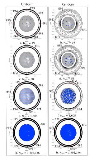
Figure 1: Sphere packing and the equilibrium points [5].

SPH-Mas Gravity Model: The gravity of an irregular shape body is modelled with a cluster of spheres, SPH-Mas. Each spherical particle contributes in the overall gravity field of the body. The exterior gravity potential of each sphere behaves as a single point mass. The potential of the irregular body is the result of the summation of each point mass’s potential that contributes to the overall potential field such that:

                                                                                     (1)

where  m_i (i = 1, ..., N_sph) is the mass of each SPH-Mas for a total of N_sph masses. r is the distance from the field point and the center of the asteroid. r_i is the distance of each masses with respect to the center of the asteroid. The total mass of the asteroid is conserved and given by m_b = ∑_{(i = 1,.., Nsph)} m_i.

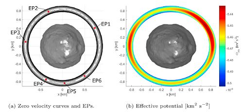
Figure 2: Shape model [1] and the equilibrium points.

Sphere Packing: We consider Ryugu’s polyhedron model published in [1] as our “high fidelity” gravity model. We distribute the SPH-Mas within the asteroid shape such that we can approximate Ryugu’s “high fidelity” gravity field. For the scope of testing our semi-analytic formula, we compared a uniform sphere packing approach with a random packing approach for different numbers of SPH-Mas. Fig. 1 shows the comparison between the uniform distribution in the left panel and the random distribution in the right panel for N_sph = 19, 58, 1,605 and 1,406,146. By comparing the location of the EPs between Fig 1 and Fig 2, it is clear that under the assumption of uniform density polyhedron, the uniform sphere packing is preferable to the random sphere packing even for the case of N_sph major to the order of million spheres. Indeed, the random sphere packing does not necessarily preserve the geometry of the EPs that affects the ejecta dynamics.

Effect of SPH-Mas Packing onto Particles Dynamics: The derived semi-analytical formula based on an SPH-Mas gravity model is a direct function of the sphere packing distribution (density), their position (r_i) and the asteroid’s spin axis angular velocity (7.6 h for Ryugu) which allows to find families of periodic orbits for ejecta particles around an non-uniform irregular shaped asteroid as shown in Fig 3.

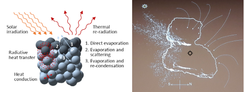
Fate of Ryugu’s Ejecta: We made use of goNEAR tool to simulate the dynamics of 10 cm, 5 cm, 1 cm and 1mm in diameter size particles under the effect of the solar radiation pressure perturbation. In the numerical experiment, few particles seemed to survive in orbit for diameter of 5–10 cm (Fig 4). The search for evidence of particles in Ryugu orbit is still unconfirmed however the stability of EPs can be linked to long survival particles in orbit.

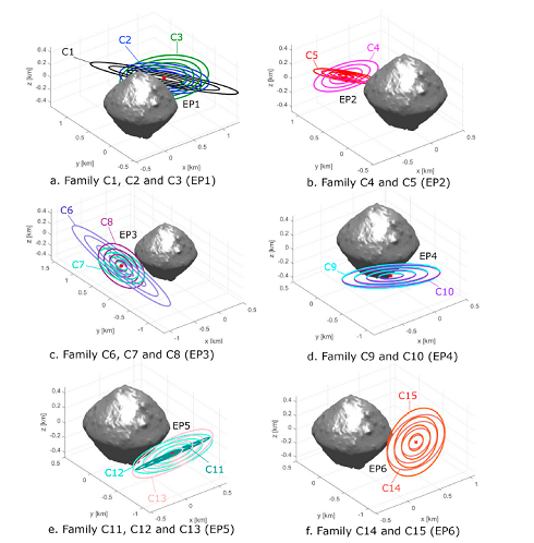
Figure 3: Family of periodic orbits as function of sphere packing [5].

Figure 4: SCI’s ejecta dynamics with the goNEAR tool [5].

References: [1] Watanabe et al. (2019) Science, 364, 268–272. [2] Lauretta et al. (2015) Meteoritics & Planet. Sci., 50, 834–849. [3] Sugita et al. (2019)  Science, 364, 6437. [4] Arakawa et al. (2019) Science, under review [5] Soldini et al, (2019) PSS, (2020) 180 [6] Melosh et al., (2013) Science, 340,1552–1555 [7] Ballouz et al., (2018) 49^th LPSC.

How to cite: Soldini, S., Saiki, T., Ikeda, H., Wada, K., Arakawa, M., and Tsuda, Y.: The effect of "MASCONS" Sphere Packing onto the Dynamical Environment around Rubble-Pile Asteroids: Application to Ryugu, Europlanet Science Congress 2020, online, 21 Sep–9 Oct 2020, EPSC2020-808, https://doi.org/10.5194/epsc2020-808, 2020.

Introduction

Asteroid (16) Psyche is the largest M-type asteroid in the main belt and the only metal rich asteroid of this size (D > 200 km). It has been proposed that Psyche could be an exposed planetary core [S17,D18]. This hypothesis and the uniqueness of Psyche's characteristics are the main reasons for its selection as the rendez-vous target of a NASA Discovery mission that is scheduled to launch in 2022 [E17].

However, the true nature of Psyche remains enigmatic which leads to the formulation of several distinct formation scenarios. Psyche’s density appears compatible with that of stony-iron meteorites such as mesosiderites [Vi18] as well as that of pallasites and CB chondrites [E20]. It is also unknown if its interior is intact or a is a rubble pile and if it is differentiated.

Observation

We obtained 35 images of Psyche at 7 epochs in July and August 2019 using VLT/SPHERE/ZIMPOL. They complement the first 25 images obtained in 2018 that were already presented in [Vi18], for a total of 60 images taken at 12 epochs. Psyche was observed near opposition with a pixel size corresponding to ~6 km/px. The first apparition in 2018 was limited to the northern hemisphere of Psyche but the second apparition in 2019 covered well the equatorial region and allowed us to achieve a complete coverage of the surface.

Methods

First, we generated an updated shape model of Psyche with the ADAM inversion algorithm [Vi15]. We used the same procedure as in [Vi18] and added the new SPHERE images and a new stellar occultation recorded in October 2019.

We then applied our Multi-resolution PhotoClinometry by Deformation (MPCD; [C13]) method on a selection of the SPHERE images to reconstruct the 3D shape of Psyche. The MPCD software gradually deforms the vertices of an initial mesh to minimize the difference between the observed images and realistic images of the surface. The ADAM model was used as input for the initial mesh and the spin parameters.

Results and conclusions

The ADAM and MPCD shape models are remarkably similar with a small volume difference and radial differences mean. The comparison between the SPHERE images and the corresponding synthetic images is given in Fig. 1. The densities derived from the volumes of both shape models combined with the average of available mass estimates are close to ~4 g/cm³ which is in agreement with other recent estimates [S17,D18,Vi18].

A shape analysis was performed by computing the radial differences between Psyche’s shape model and its best-fitting ellipsoid to obtain the average residuals relative to the mean radius. We then computed the sphericity index of Psyche using the same approach as in [V19]. We repeated the process for other large main-belt asteroids, the terrestrial planets and smaller asteroids visited in-situ by space missions. It revealed that Psyche’s shape appears intermediate between those of larger asteroids and those of smaller or similarly sized bodies. Psyche’s appearance is close to an ellipsoid with flat regions at the poles even though we identified three depression regions along its equator.

Finally, we investigated whether the shape of Psyche may be close to the equipotential shape of an hydrostatic body. The flatness and density of Psyche are compatible with a formation at hydrostatic equilibrium as a Jacobi ellipsoid with a shorter rotation period of ~3 h. Later impacts may have slowed down Psyche’s rotation, which is currently ~4.2 h, while also creating the imaged depressions. Our results open the possibility that Psyche acquired its primordial shape either after a giant impact while its interior was already frozen or while its interior was still molten owing to the decay of the short-lived radionuclide ²⁶Al.

Figure 1: Comparison between VLT/SPHERE/ZIMPOL deconvolved images of Psyche (top row) and the corresponding synthetic images of our MPCD (second row) and ADAM (third row) shape models. The red arrows indicate the direction of the spin axis.

Bibliography

[C13] Capanna, C., Gesquière, G., Jorda, L., Lamy, P., & Vibert, D. 2013, The Visual Computer, 29, 825

[D18] Drummond, J. D., Merline, W. J., Carry, B., et al. 2018, Icarus, 305, 174

[E17] Elkins-Tanton, L. T., Asphaug, E., Bell, J. F., et al. 2017, in Lunar and Planetary Science Conference, Lunar and Planetary Science Conference, 1718

[E20] Elkins-Tanton, L., Asphaug, E., Bell, J., et al. 2020, Journal of Geophysical Research: Planets

[S17] Shepard, M. K., Richardson, J., Taylor, P. A. et al. 2017, Icarus, 281, 388

[V19] Vernazza, P., Jorda, L., Ševecek, P., et al. 2019, Nature Astronomy, 477

[Vi15] Viikinkoski, M., Kaasalainen, M., & ˇ Durech, J. 2015, A&A, 576, A8

[Vi18] Viikinkoski, M., Vernazza, P., Hanuš, J., et al. 2018, A&A, 619, L3

How to cite: Ferrais, M., Vernazza, P., Jorda, L., Rambaux, N., and Hanuš, J. and the HARISSA team: Asteroid (16) Psyche's primordial shape: A possible Jacobi ellipsoid, Europlanet Science Congress 2020, online, 21 Sep–9 Oct 2020, EPSC2020-289, https://doi.org/10.5194/epsc2020-289, 2020.

Asteroid mass determination is performed by analyzing an asteroid's gravitational interaction with another object, such as a spacecraft, Mars, a companion in the case of binary asteroids, or a separate asteroid during a close encounter. During asteroid-asteroid close encounters, perturbations caused by the masses of larger asteroids can be detected in the post-encounter orbits of the smaller test asteroid involved in such an encounter. This can be described as an inverse problem where the aim is to fit six orbital elements for each asteroid and mass(es) for the perturbing asteroid(s), for a total of 13 parameters at minimum unless more asteroid-asteroid encounters are modeled simultaneously.

To solve this inverse problem, which is traditionally done with least-squares methods, we have implemented a Markov-chain Monte Carlo (MCMC) based solution and recently (Siltala & Granvik 2020) reported, among others, significantly lower than expected masses and densities for the asteroid (16) Psyche in particular. Psyche is an interesting, and topical, object as it is the target of NASA's eponymous Psyche mission and is commonly thought to be of metallic or stony-iron composition, which our previous density estimates disagreed with. In our previous work our two separate mass estimates for Psyche were based on modeling encounters with two separate test asteroids in both cases. Since then we have further refined our mass estimate for Psyche by simultaneously using eight separate test asteroids for this object, significantly increasing the amount of observational data included on the model which, in turn, will narrow down the uncertainties of our results at the cost of additional model complexity. Here we report and discuss our latest results for the mass of Psyche based on this case and compute corresponding densities based on existing literature values for the volume. We obtain a mass of (0.972 ± 0.148) * 10^-11 solar masses for Psyche corresponding to a bulk density of (3.37 ± 0.58) g/cm³ which is higher than our previous results while remaining consistent with them considering the uncertainties involved. It still remains lower than other previous literature values. We compare our results to these previous literature values and briefly discuss possible physical implications of these results.

In addition, due to previous interest from the scientific community, we have also computed mass estimates for Ceres and Vesta, both of which already have very precisely known masses from the Dawn mission. As such, our results for these two asteroids are not of direct scientific interest but they serve as an useful benchmark to verify that our algorithm provides realistic results as we have 'ground truth' values to compare our results to. We find that for both cases, our results are in line with those of Dawn.

How to cite: Siltala, L. and Granvik, M.: New estimates of the mass and density of asteroid (16) Psyche, Europlanet Science Congress 2020, online, 21 Sep–9 Oct 2020, EPSC2020-752, https://doi.org/10.5194/epsc2020-752, 2020.

INTRODUCTION

Comet 67P/C-G is a dusty object. As it neared its closest approach to the Sun in late July and August 2015, instruments on Rosetta recorded a huge amount of dust enshrouding the comet. This is tied to the comet’s proximity to our parent star, its heat causing the comet’s nucleus to release gases into space, lifting the dust along [10]. Spectacular jets were also observed, blasting more dust away from the comet. This disturbed, ejected material forms the ‘coma’, the gaseous envelope encasing the comet’s nucleus, and can create a beautiful and distinctive tail. A single image from Rosetta’s OSIRIS instrument can contain hundreds of dust particles and grains surrounding the 4 km-wide comet nucleus.

The study of the dust behaviour is vital for understanding the global evolution of the comet and has direct consecuences in the research of the origins of the solar system. [1]

That helps for calculating the average mass loss rate per period. Calculations are not so simple since two situations may occur. The diurnal thermal cycle plus the irregularities in the shape of the comet produces a flow of particles from the southern hemisphere to the northern and most particles are redeposited. However some areas, like Hapi region, are eroded around 1.0± 0.5 m per orbit. Some other areas are growing with deposits of dust creating moving shifting dunes. It is believed the 95% of the ejected dust particles are falling back into the comet.

DUST ANALYSIS

A simple image of the OSIRIS instrument can contain hundreds of dust and grain particles around a 4km sphere around the core. The images above show the level of complexity when processing an image. Partly, most image sequences are processed manually [5]

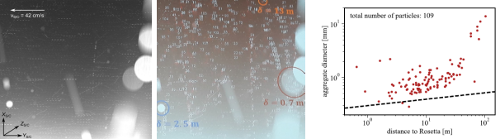
The largest particle that has been observed on the surface of the comet is at least 20 x 30 x 40 m in size and displaced by a distance of 140 m [4].

BIG BOULDERS

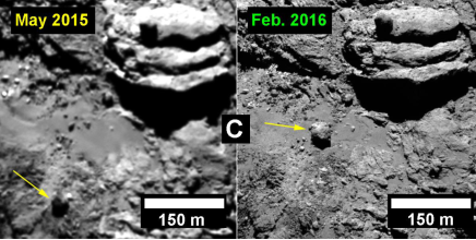
Sometimes, even larger chunks of material left the surface of 67P/C-G – as shown here. The sizeable chunk in this view was spotted a few months ago by astrophotographer Jacint Roger from Spain, who mined the Rosetta archive, processed some of the data, and posted the finished images on Twitter as an animated GIF. He spotted the orbiting object ina sequence of images taken by Rosetta’s OSIRIS narrow-angle camera on 21 October 2015. At that time, the spacecraft was at over 400 km away from 67P/C-G’s centre. The trajectories have been calculated with Trackmate [7] and SPICE [9]. The location of the particles in the image list of the instrument is complicated due to the large number of particles that the images contain. 

This particle was nicknamed Churymoon and at present its trajectory,orbital stability [8] is being studied as the consecuences of this discovery.

Following the methodology explained in [5], we can determine the size of Churymoon. Assuming that the photometric properties of the particle are the same as those of the nucleus, the total brightness of the particle divided by the total brightness of the comet per pixel gives us the fraction of pixels occupied by the particle.

The result, 3.9 meters in effective diameter, making Churymoon the largest 67P ejected particle ever detected.

^{* The size could be slightly overestimated by the calculation method used (ice or glitter in the core).}

METHODOLOGY

There is no universal method for calculating dust trajectories in comets [7]. To date, studies have been carried out on: trajectories close to the surface of the comet [2], in the first image; calculation of trajectories through parallax between two cameras on board Rosetta [13], [15], [16], in the second image; and orbital determination for long periods of time [11], in the third image. To determine Churymoon's trajectory, neither of these methods would work individually, but a combination of them could be effective:

Using the satellite's displacement as a parallax source, in the fourth image, the position and velocity could be determined if the particle remains long enough in the camera's field of view

This method has been automatically tested on other image sequences, in the last illustration, effectively solving the trajectories. The biggest drawback is the large number of false positives (stars, cosmic rays, etc ...) that make real detections difficult.

CONCLUSSIONS

The implications of discovering a particle like this suggest new unknowns:

• These particles would describe trajectories following the comet's rotation. If so, there would be a restriction in determining the distance assuming a pure radial motion.
• If the particle production ratio of more than one meter was high enough, they could be relevant in calculating the total production of gas and dust. The search for possible future Churymoons is vital
• In principle, the contribution of these particles to the early disappearance of the near-earth asteroid population would be very small (~ 2.5%), but this is not conclusive.

BIBLIOGRAPHY

[1] Fulle et al 2016

[2] Agarwal et al 2016

[3] Guttler et al 2016

[4] El Maary et al 2017

[5] Guttler et al 2017

[6] Timenez et 2017

[7] Chenuard N et al 2014.

[8] Bertini et al 2015

[9] DOI: 10.5270/esa-tyidsbu

[10] Blum et al 2015

[11] Davidsson et al 2016

[12] Bertini et al 2017

[13] Drolshagen & Ott et al 2017

[14] Davidsson et al 2015

[15] Drolshagen et al 2017

[16] Ott et al 2017

[17] Ott (IMC 2016)

How to cite: Marín-Yaseli de la Parra, J., Kueppers, M., Roger Pérez, J., and Osiris Team, T.: Analysis of a particle in the surroundings of 67P, Europlanet Science Congress 2020, online, 21 Sep–9 Oct 2020, EPSC2020-801, https://doi.org/10.5194/epsc2020-801, 2020.

An apparent discrepancy between the number of observed near-Earth objects (NEOs) with small perihelion distances (q) and the number of objects that models
predict, has led to the conclusion that asteroids get destroyed at non-trivial distances from the Sun. Consequently, there must be a, possibly thermal,
mechanism at play, responsible for breaking up asteroids asteroids in such orbits.

We studied the dynamical evolution of ficticious NEOs whose perihelion distance reaches below the average disruption distance q_dis=0.076 au, as suggested by
Granvik et al. (2016). To that end, we used the orbital integrations of objects that escaped from the main asteroid belt (Granvik et al. 2017), and entered the
near-Earth region (Granvik et al. 2018). First, we investigated a variety of mechanisms that can lower the perihelion distance of an object to a small-enough
value. In particular, we considered mean-motion resonances with Jupiter, secular resonances with Jupiter and Saturn (v_5 and v_6) and also the Kozai resonance.

We developed a code that calculates the evolution of the critical argument of all the relevant resonances and identifies librations during the last stages of
an object's orbital evolution, namely, just before q=q_dis. Any subsequent evolution of the object was disregarded, since we considered it disrupted. The
accuracy of our model is ~96%.

In addition, we measured the dynamical 'lifetimes' of NEOs when they orbit the innermost parts of the inner Solar System. More precisely, we calculated the
total time it takes for the q of each object to go from 0.4 au to q_dis (τ_lq). The outer limit of this range was chosen such because it is a) the approximate
semimajor axis of Mercury, and b) an absence of sub-meter-sized boulders with q smaller than this distance has been proposed by Wiegert et al (2020). Combining
this measure with the recorded resonances, we can get a sense of the timescale of each q-lowering mechanism.

Next, for a more rigorous study of the evolution of the NEOs with q<0.4 au, we divided this region in bins and measured the relevant time they spend at
different distances from the Sun. Together with the total time spent in each bin, we kept track of the number of times that q entered one of the bins.
Finally, we computed the actual time each object spends in each bin during its evolution, i.e., the total time it spends in a specific range in radial
heliocentric distance.

By following this approach, we derived categories of typical evolutions of NEOs that reach the average disruption distance. In addition, since we have the
information concerning the escape route from the main asteroid belt followed by each NEO, we linked the q-lowering mechanism and the associated orbital
evolutions in the range below the orbit of Mercury, to their source regions and thus were able to draw conclusions abour their physical properties.

How to cite: Toliou, A. and Granvik, M.: Dynamical evolution of near-Earth objects, Europlanet Science Congress 2020, online, 21 Sep–9 Oct 2020, EPSC2020-1104, https://doi.org/10.5194/epsc2020-1104, 2020.

Based on previous applications of laser altimetry to planetary geodesy at GSFC [Mazarico et al. (2014)], we use the recently developed PyXover software package to analyze altimetric crossovers from the Mercury Laser Altimeter (MLA) and improve geodetic parameters via least squares (LS) minimization of crossover discrepancies.
We simultaneously solve for orbital corrections for each MESSENGER track, for the geodetic parameters of the IAU recommended orientation model for Mercury [Archinal et al, 2018], and for the Mercury Love number h₂.
We calibrate the formal errors of our solution based on closed-loop simulations and on the level of independence from \emph{a priori values and data selection.

Data description:

From  March  2011  to  April  2015, the MESSENGER spacecraft orbited Mercury in a highly elliptical, near-polar orbit with a periapsis of ~200-400 km, an apoapsis between ~1.5-2 x 10^4 km, and an orbital period of 12 hrs initially and reduced  to  8  hrs  after  one  year. The spacecraft was  within  ranging  distance for the onboard MLA over  15-45 min periods near periapsis, typically at latitudes > 30 deg N.

MLA collected over 22 million measurements of surface height with a vertical precision of ~1 m and an accuracy of ~10 m. The total MLA dataset contains ~3,200 tracks and ~3 million crossovers, i.e., instances where  two  ground-tracks  intersect.  Because  of  the  elliptical  orbit,  the  laser spot  size  on  the  surface  varied  between ~10 - 100 m, while  the average distance  between each  crossover and its bracketing observations was ~200 m.

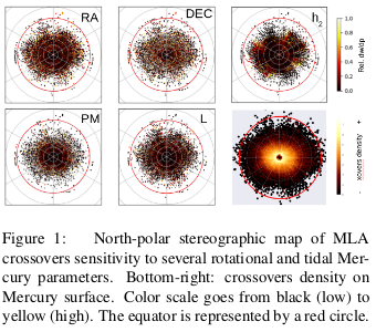
These  crossovers provide an opportunity to measure Mercury’s  orientation  and  rotation (see Fig.1).
Independent  confirmation  and  refinement  of  the IAU  libration  model,  developed  from  ground-based radar measurements [Margot et al. 2009], is important as it has implications  for  the  moment  of  inertia  of  the  outer  solid  shell and  thus  the  mass  distribution,  internal  structure,  and thermal  evolution  of  Mercury [Phillips et al. (2018), Genova et al. (2019)].

Processing and solution strategy:

Each  crossover  is  the  intersection  of  two  separate 
ground-tracks. It can be thought of as a differential measurement between two  distinct  observations of the same surface location at two different 
times. Any  difference  in  height  at the crossover  point  is  mainly due to the following  effects: 
(1)  Errors  in  the spacecraft  orbit and  attitude, or MLA  boresight  orientation,  (2)  interpolation  errors  of the surface topography between MLA footprints, and (3) geophysical signal due, e.g., to mismodeled  time-varying  planetary  rotation or to tidal vertical motions.

We perform the analysis of MLA data with the PyXover python code, whose modular structure is sketched in Fig.2.
Laser altimetry ranges are geolocated to the planetary surface and partial derivatives of the ground-tracks are computed with respect to the chosen parameters by finite differencing. Initial geolocation is based on the MESSENGER orbit navigation reconstruction by KinetX and on the values provided by the IAU for Mercury orientation [Archinal et al, 2018]. Values for the Love numbers h₂ and l₂ are set to 0 in our a priori tidal model.
Horizontal coordinates of crossover points are recovered in local stereographic projection in a two-step process, to balance computational time.
Expected elevations at intersection points are then interpolated from neighbouring points on each track. Their discrepancies w constitute the observation residuals to be minimized in the LS procedure.
Huber weighting is then applied to the crossovers depending on the reliability of the orbital tracks involved, on the off-nadir angle of the spacecraft and on inter-point distances. Crossovers with abnormally large discrepancies are strongly down-weighted in our analysis. 
We minimize the total RMSE of crossover discrepancies within a penalised LS with weights determined by Variance Component Estimation (VCE). 
The resulting corrections to MESSENGER orbits and Mercury geodetic parameters are then applied to update the a priori for the subsequent iteration, until convergence is reached.

Parametrization and error assessment:
Formal errors provided by LS and VCE are notoriously under-estimated. We thus perform additional analysis to consider systematic error sources, such as the chosen apriori values and data selection. In particular, we measure the stability of the solutions resulting from different Doppler reconstructions of MESSENGER orbits (KinetX and [Genova et al, 2018]) and from both IAU [Archinal et al, 2018] and [Genova et al, 2019] values for Mercury rotational parameters. Also, we process multiple sub-samples of 500,000 crossovers (max 20% in common, stratified by latitude to conserve the overall geographical distribution) and we verify the dispersion of the solutions at convergence.
Moreover, we conduct extensive simulations with time-of-flight ranges consistently generated from realistic topography to analyze the impact of the interpolation error and the reliability of the recovery in different scenarios and parametrizations. 

Processing of MLA crossovers:

Finally, we perform a weighted LS solution of orbit corrections and geodetic parameters based on the presented processing setup.
We base our solution on a set of 10⁶ crossovers selected according to their computed weight (i.e., their quality) and to ensure a balanced geographical distribution. 
We iterate the solution until convergence is reached, i.e., parameters changes are well below formal errors (<10 iterations). Observation weights are re-evaluated at each iteration down to the convergence of discrepancies RMSE at 5% and then fixed.

We check the reduction of the RMSE of post-fit discrepancies w, as shown in Fig.3, the evolution of VCE derived weights and the consistency of topography maps to evaluate the improvements.

Our results for some geodetic parameters are shown in Fig.4 and are consistent with previous solutions provided by other groups using various techniques (camera and altimetry, Doppler, Earth-based radar). 

Error bars are calibrated based on both closed-loop simulations and the analysis of systematic errors outlined in the previous section.
We will discuss the recovered h₂ and our determination of Mercury rotational parameters at the meeting.

Acknowledgements
S. Bertone acknowledges support by the Swiss National Science Foundation within the Advanced Postdoc Mobility program and by NASA’s Planetary Science Division Research Program through the CRESST II cooperative agreement. The MLA data were processed on the GSFC NCCS ADAPT cluster.

How to cite: Bertone, S., Mazarico, E., Barker, M. K., Goossens, S., Neumann, G. A., Sabaka, T. J., and Smith, D. E.: Latest update of Mercury geodetic parameters with altimetric crossovers from the Mercury Laser Altimeter (MLA), Europlanet Science Congress 2020, online, 21 Sep–9 Oct 2020, EPSC2020-525, https://doi.org/10.5194/epsc2020-525, 2020.

Knowing if the inclination of a satellite with respect to the equator of its planet is primordial can give hints on its origin and its formation. However, several mechanisms are able to modify its inclination during its evolution. The orbit of a satellite evolves over time and because of the tidal dissipation its semi-major axis can notably decrease or increase. Therefore the satellite can encounter several resonances in which it can potentially be captured. Some resonances are able to modify the equatorial inclination of a satellite. Touma and Wisdom (1998) noted that a resonance called ‘eviction’ between the mean motion of the Earth and the ascending node frequency of the Moon could increase by several degrees the equatorial inclination of the early Moon and could explain the present orientation of its orbit. Yokoyama (2002) studied these resonances for Phobos and Triton and observed that several resonances of this type can increase the equatorial inclination of Phobos in the future.

In this work, we study the different existing ‘eviction’ resonances to determine their possible influence on the equatorial inclination of a satellite. When a satellite goes through such a resonance, the capture is not certain and as noted by Yokoyama (2002), the probability of capture depends on several parameters as the obliquity of the planet and the interaction between other resonances. We consider the case of Phobos where we search to estimate the probability of a capture in an ‘eviction’ resonance by using an analytical Hamiltonian model and numerical simulations. This work will then notably estimate the probability that Phobos will be captured in the future in an ‘eviction’ resonance able to modify significantly its inclination and will measure the influence of the different parameters over the probability of capture.

Acknowledgments: The authors acknowledge support from project POCI-01-0145-FEDER-029932 (PTDC/FIS-AST/29932/2017), funded by FEDER through COMPETE 2020 (POCI) and FCT.

References:

Touma J. and Wisdom J., Resonances in the Early Evolution of the Earth-Moon System. The Astronomical Journal, 115:1653–1663, 1998.

Yokoyama T., Possible effects of secular resonances in Phobos and Triton. Planetary and Space Science, 50:63–77, 2002.

How to cite: Vaillant, T. and Correia, A. C. M.: Influence of some resonances on the inclination of a satellite, Europlanet Science Congress 2020, online, 21 Sep–9 Oct 2020, EPSC2020-440, https://doi.org/10.5194/epsc2020-440, 2020.

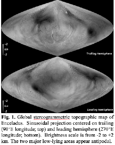
Cassini observations have led to several efforts to map the global topography of Enceladus [1-5]. The most prominent large-scale features include 100+ km scale basins (1), and the depressed south polar terrain (SPT) [2]. Here we present a revised and complete stereogrammetric map of Enceladus topography at 0.4-km scales (Fig. 1) including the north polar regions mapped at the end of the mission and that does not require interpolation. We reevaluate the distribution and origin of large-scale topographic deviations and compare north and south polar regions.

Stereogrammetric digital elevation models (DEMs) of Enceladus were constructed from Cassini stereo pairs and mosaics using the same software used to map the topography of Pluto, Charon, and other icy bodies [6].  As each stereo pairing has a unique stereo geometry, the vertical precision (or uncertainty) is variable across Enceladus and ranges from <50 to ~300 m.  Hence while most DEMs resolve geologic features, a few do not. The individual stereo-DEMs are assembled into a global DEM (Fig. 1) by minimizing the difference to our (coarser but coincident) map of 4591 match point radii values.  Our new map shows topography relative to the triaxial ellipsoid of [2].  Here we focus on global and regional variations and defer analyses of geologic features.

Schenk and McKinnon [1] discovered several oval-shaped depressions on the trailing hemisphere circa 150-km across and 1-1.5 km deep in their partial DEM.  They found an isostatic explanation for these depressions to be most physically plausible, and concluded that basins could be sites of cold, dense, immobile (or downwelling), partially clathrated ice, or alternatively, manifestations of deeper convective upwellings (and porosity reduction), either now or in the past. Tajeddine et al. [4] extended the global topography map through a spherical harmonic representation (to degree 16) based on both limb profiles [2] and stereogrammetric control points, and reported that additional depressions occurred on the remaining surface and that some formed an apparent great circle; [4] further suggested the circle was offset due to true polar wander (TPW).  Our new map is much denser in terms of stereo-derived elevations, yielding ~5.2×10⁶ measurements, spaced every 0.4 km or so.  We find that Enceladus’ surface topographic signature is both complex and subtle. Contrary to our expectations [1], no additional deep basins similar to those reported by [1] occur in the leading hemisphere.

Without these basins the case for a great circle alignment (and by extension any TPW implied) is weakened. We also note that the average ice shell thickness of ~20-25 km implied by Enceladus’ libration [7] does not easily support a convective origin for the “E basins” proposed by [4]; the present-day shell is too thin [cf. 8].

The circular resurfaced zone that dominates the leading hemisphere [9] has a warped signature suggestive of large rounded polygons separated by elongate depressions.  Some of the highest elevations occur in the southern part of this resurfaced zone. The topographic signature of the trailing hemisphere zone is different again.  Neither exhibit the concentric rings that might be expected from topographic relaxation or thickening of a region similar to the current depressed SPT, if they were once active in a similar way and ceased thermal activity. The two resurfaced zones may have responded differently to regional stresses than the older cratered terrains between them. 

2. North vs. South Polar Terrains

A fundamental characteristic of Enceladus is that the SPT is vigorously resurfacing and active but the cratered northern polar terrains (NPT) are not despite models that show similar tidal heating at both poles [10]. The NPT were the last areas to be mapped by Cassini. Our global DEM confirms that the SPT (>70°S) is depressed ~400 m relative to the best-fit ellipsoid (confirming [2]), but the NPT (>70°N) are elevated ~0.7 km above. The north polar imaging confirms that tectonic features with fresh blue-ice signatures do cross the NPT. The apparent broad doming of the NPT might suggest that either the ice shell is relatively thick there (and perhaps more resistant to tidal heating relative to the original southern terrain) or that incipient resurfacing is preceded by doming before the crustal replacement cycle begins.

3. Global Aspects and Conclusions

A global hypsogram of Enceladus (Fig. 2) using our new complete DEM (Fig. 1) shows that global topographic deviations from the first-order triaxial ellipsoid [2] are at the 95th percentile within ±1 km of the triaxial ellipsoid, confirming earlier incomplete maps [1,4]. Two ‘humps’ can be identified in the hypsogram at -0.4 km (representing the SPT) and at -1 km (representing the basins). This is possibly the narrowest global topographic signature in the Solar System for an ellipsoidal body [11], although it might be matched by Europa, Ganymede and Triton (work in progress), and is consistent with expected subdued topography of an active icy ocean world. The preservation of the deep 1-1.5 km deep basins is an unsolved problem [1,3], but might reflect patterns of heat flow from the core [12].  Enceladus’ topographic signature is complicated, with indications that older cratered terrains and the three younger resurfaced terrains responded differently to stresses.  The distribution of large deep basins is enigmatic, and although they do not form a great circle, lower-lying topography is more prevalent at mid-northern latitudes.  More complete analyses of higher harmonics are underway and may yield additional insights.

References

[1] Schenk, P., and McKinnon, W., GRL 36, L16202, 2009. 

[2] Thomas, P.C, et al., Icarus 190, 573–584, 2007.

[3] Nimmo, F., et al., JGR 116, E11001, 2011.

[4] Tajeddine, R., et al., Icarus 295, 46-60, 2017.

[5] Bland, M., et al., 4^th Planetary Data Workshop, abs. #7048, 2019.

[6]. Schenk, P.M., et al., Icarus, 314, 400-433, 2018a.

[7] Thomas, P.C, et al., Icarus 264, 37-47, 2016.

[8] Barr A.C., and McKinnon, W.B., GRL 34, L09202, 2007.

[9]. Crow-Willard, E., R. Pappalardo, JGR., 120, 928-950.

[10] Nimmo, F., et al., in Enceladus and the Icy Moons of Saturn, UA Press, pp. 79-94, 2018.

[11] Schenk, P., et al., in Enceladus and the Icy Moons of Saturn, UA Press, pp. 237-265, 2018.

[12] Čadek, O., et al., Icarus 319, 476-484, 2019.

How to cite: Schenk, P. and McKinnon, W.: Global Topography of Enceladus: North-Pole-South-Pole, Deep Basins and TPW Revisited, Europlanet Science Congress 2020, online, 21 Sep–9 Oct 2020, EPSC2020-497, https://doi.org/10.5194/epsc2020-497, 2020.

Io, the innermost of Jupiter’s satellites, is the most volcanically active, and probably one of the most remarkable body in the outer Solar System [1]. The total power emitted from Io's surface is estimated to about 100 TW at present [2,3], which is several orders of magnitude greater than can be explained by radiogenic heating alone. Io’s interior process manifests on the surface as extreme volcanic activity, providing some clues about the thermal state of its interior through the eruption properties and global distribution of volcanism [e.g. 4,5].

A variety of models have been proposed to determine the mechanism at the origin of the huge tidal dissipation in Io’s interior [e.g. 6,7,8,9]. The presence of a partially molten layer in the upper mantle of Io is broadly consistent with these interior models prediction, as well as with magnetic induction measurements [10], although this interpretation has recently been questioned [11]. However, while a high concentration of melts below the lithosphere is in line to explain the heat production and the heat released by volcanic activity, the degree of melting of this subsurface layer, going from moderately molten mantle to fully liquid subsurface ocean [7], is still largely debated.

The distribution of melt within Io is a key question driving future mission concept dedicated to Io’s investigation (IVO), planning to test these interior models via a set of geophysical measurements. One way to characterize it is through the tides. The measurement of the tidal deformation (either via the potential Love number k2 or the phase lag) can provide information about the internal structure of planetary bodies [e.g. 12].

The total amount of heat produced by tidal friction and its distribution in the interior is intimately linked to the structure and thermal state of Io's interior, especially the distribution of temperature and melt fraction [8,9]. Describing the mechanical response of partially molten rocks on a wide range of melt fraction is essential to correctly describe the tidal friction in Io, partial melt severely affecting viscoelastic properties of rocks. Understanding the retroaction between melt distribution and heat production is thus crucial to explain the heat budget of Io and to understand its tidally-induced volcanism.

In this context, the goal of the study is to calculate the tidal response of Io’s interior [13] for various distribution of melt within the mantle, to discriminate them in future tidal monitoring. A coherent melt profile between the sublithospheric partially molten layer and the underlying mantle is considered following petrological and two-phase flow arguments [4,14]. A rheological parameterization is developed in order to take into account the role of melt fraction on the elastic and viscous parameters of Io's partially molten interior. The results are analyzed in terms of tidal Love number k₂, taking into account a re-evaluation of the heat production by tidal friction in Io's partially molten interiors, by quantifying the role of melt fraction on both shear and bulk dissipation.

Our calculations show that the amount of melt fraction within the 100-km thick asthenospheric partially molten layer could be discriminated from tidal k₂ measurements and heat flow patterns. Depending on the assumed value of viscosity at the melting point and extent of melting beneath the lithosphere, three groups of internal structure models able to reproduce Io’s heat budget of 100 TW can be distinguished : (1) low viscosity mantle (<10¹⁷ Pa s) and moderately molten mantle and asthenosphere (<7%-<20% respectively) ; (2) high viscosity mantle (>10¹⁸ Pa s) with high melt content in the asthenosphere (>30%) ; (3) fully liquid magma ocean beneath a highly dissipative crust. Both mantle dissipation (1) and crust dissipation (2) models result in a comparable heat flow pattern, with maximal dissipation at the poles but can be distinguished by k₂ measurements. The asthenospheric dissipation (2) model has a k₂ Love number only slightly higher than the mantle dissipation model, but results in a totally different heat flow pattern. Note that our computed dissipation included bulk dissipation in addition to shear dissipation, which further enhances dissipation in the equatorial region for the asthenospheric dissipation (2) model. For the two other dissipation model, bulk dissipation has a negligible effect. 

Acknowledgements

The present work received financial supports from the ANR OASIS project and from CNES (Europa Clipper/SUDA, JUICE).

References

[1] Lopes, R. M., and Williams, D. A., Io after Galileo. Reports on Progress in Physics, 68(2), 303 (2005).
[2] Veeder, G. et al., JGR: Planets, Vol. 99, pp. 17095-17162 (1994).
[3] Spencer, J. et al., Eos Trans AGU, Vol. 81,  pp. 19 (2000).
[4] Keszthelyi, L., Jaeger, W., Milazzo, M., et al. 2007, Icarus, 192, 491
[5] Davies, A. G., G. J. Veeder, D. L. Matson, and T. V. Johnson (2015), Icarus, 262, 67–78
[6] Segatz, M. et al., Icarus, Vol. 75, pp 187-206 (1988).
[7] Tyler, R. H., W. G. Henning, and C. W. Hamilton (2015), Astrophys. J. Suppl. Ser., 218(2), 22.
[8] Bierson, CJ. and Nimmo, F., JGR: Planets, Vol. 121, pp 2211-2224 (2016).
[9] Steinke, T., Hu, H., Höning, D., van der Wal, W., & Vermeersen, B. 2020, Icarus,335, 113299
[10] Khurana, K. et al., Science, Vol. 332, pp. 1186-1189 (2011).
[11] Roth, L., Saur, J., Retherford, K. D., et al. 2017, Journal of Geophysical Research: Space Physics, 122, 1903
[12] Dumoulin, C. et al., JGR : Planets, Vol. 122, pp. 1338 1352 (2017)
[13] Tobie, G. et al., Icarus, Vol. 177, pp. 534-549 (2005).
[14] Spencer, D. C., Katz, R. F., & Hewitt, I. J. 2020, arXiv preprint arXiv:2003.08287
[15] de Kleer, K., Park, R., McEwen, A.S. Tidal heating: Lessons from Io and the Jovian System Final report (2019)

How to cite: Kervazo, M., Tobie, G., Choblet, G., Dumoulin, C., and Běhounková, M.: Inferring Io's interior from tidal monitoring , Europlanet Science Congress 2020, online, 21 Sep–9 Oct 2020, EPSC2020-598, https://doi.org/10.5194/epsc2020-598, 2020.