Europlanet Science Congress 2020
Virtual meeting
21 September – 9 October 2020
Europlanet Science Congress 2020
Virtual meeting
21 September – 9 October 2020

Poster presentations and abstracts

TP2

Shape, gravity field, orbit, tidal deformation, and rotation state are fundamental geodetic parameters of any planetary object. Measurements of these parameters are prerequisites for e.g. spacecraft navigation and mapping from orbit, but also for modelling of the interior and evolution. This session welcomes contributions from all aspects of planetary geodesy, including the relevant theories, observations and models in application to planets, satellites, ring systems, asteroids, and comets.

Co-organized by OPS/SB
Convener: Gregor Steinbrügge | Co-conveners: Jean-Baptiste Vincent, Alexander Stark, Marie Yseboodt, Ryan Park

Session assets

Session summary

Chairperson: Gregor Steinbrügge
EPSC2020-825ECP
Lord Dover, Stephen Lowry, Agata Rożek, Tarik Zegmott, Ben Rozitis, Simon Green, Colin Snodgrass, Paul Weissman, Yurij Krugly, Irina Belskaya, and Marina Brozović

Abstract

We are conducting an observing campaign with a sample of near-Earth asteroids (NEAs) to detect YORP-induced acceleration. Photometric lightcurves from small to medium optical telescopes are used to detect changes to spin state. Where available, radar and thermal-IR observations are used to develop physical models that are used to determine expected YORP strengths. We will present the results of an analysis of 2000 PN9 (hereafter PN9) using optical and radar observations between 2001 and 2016. A detailed physical model has been developed to describe the shape and spin-state of the asteroid. PN9 is top-shaped with an equatorial ridge, and is rotating close to the spin-breakup limit. PN9 is the largest asteroid known to have this distinctive and highly symmetrical 'YORPoid' shape, and is the fastest-rotating top-shaped body that is not part of a multiple system. Due to the size and shape of PN9, an observational detection of YORP acceleration has not been possible with the available data. The shape and rotation period indicate that PN9 is a YORP-evolved body similar to 1999 KW4 [1], and that it is a good candidate for future detection of mass-lofting events.

Introduction

The YORP effect is a thermal torque caused by the reflection, absorption and anisotropic re-emission of Solar radiation [2,3]. YORP is the main driver of physical and dynamical evolution for small bodies in the inner Solar System [4]. There are seven confirmed detections of YORP to date, all of which are in the 'spin-up' mode.

The observing campaign aims to increase the number of YORP detections such that theoretical understanding of YORP can be improved. Optical and IR observations were carried out on 42 NEAs through our ESO Large Programme from 2010 to 2014, with continued monitoring conducted through associated programmes. In addition to photometric observations, thermal-IR and radar observations have been obtained for the NEA sample.

PN9 was observed in 2001, 2006, 2010, 2011, 2015 and 2016 with various optical telescopes resulting in 29 lightcurves. Radar observations were also conducted at the Arecibo and Goldstone radar facilities in 2001 and 2006. Previously published lightcurves report rotational periods around 2.53 h [5,6] and initial diameter estimates range from 1.6 - 2.0 km [5,7]. PN9 has been previously classified as an Sq-type asteroid [8].

Results & Conclusions

Detecting YORP requires well constrained measurement of the evolving rotation period and pole orientation. These parameters can be determined using lightcurve data alone, although it is beneficial to have a detailed radar shape model. This greatly assists with the computation of rotational phase offsets between observations and synthetic lightcurves derived from a constant-period shape model. YORP causes a linear change in rotation period, which in turn causes a quadratic increase in rotational phase offset against time. A radar shape model greatly assists in the detection of this quadratic trend, which is highly desirable for constraining YORP strength.

fileStorageProxy.php_1.png

Figure 1: Shape model for asteroid 2000 PN9 developed using both radar and lightcurve observations. The top row shows the model from the positive end of the Z, Y and X axes in the body-centric co-ordinate system. The bottom row shows the model from negative end of the Z, Y and X axes. 

Lightcurves of PN9 have very low amplitudes due to the highly symmetrical nature of the object. Lightcurve data alone was not sufficient to constrain the orientation of the rotational axis, so the spin-state was determined using a combination of lightcurve and radar data. Figure (2) shows the χ2 fit of pole solutions across the whole sky, with the pole-scan converging to two regions that are opposite each other on the celestial sphere. This pole solution degeneracy implies uncertainty as to whether the asteroid is a prograde or retrograde rotator. Physical models were generated for all possible pole solutions, with all solutions within 1% of the best solution having a shape and period consistent with the best solution. For the best-fit pole solution at λ=228° β=-30°, we have determined the sidereal rotation period to be 2.532972±0.000015 hours. In the body-centric coordinate system where the z-axis is aligned with the rotation axis, the maximum extents of the X, Y and Z axes are 1.885x1.888x1.780 km. As shown in Figure (1), the shape is highly symmetrical with an equatorial ridge. This shape is characteristic for a rapidly rotating rubble pile, where material is being migrated towards the equator [9] and closely resembles the convex hull model of 1917 Cuyo, a candidate for rotationally-induced mass lofting [10]. We have measured the circular polarisation ratio (SC/OC) to be 0.225±0.004, which is consistent with PN9's taxonomic type. We have been unable to measure YORP acceleration; the size and shape of PN9 results in a low expected YORP strength, and phase offsets cannot be precisely measured with relatively featureless lightcurves.

Further work that will be presented at the meeting includes an updated physical model developed with newly obtained lightcurves, and an update on Spitzer thermal-IR lightcurves of PN9.

fileStorageProxy.php.png

Figure 2: The results of a search for the rotational pole of 2000 PN9 using radar and lightcurve data. The best solution is marked with a yellow '+'. The yellow and white lines enclose regions where χ2 is within 1% and 5% of the best solution respectively.

Acknowledgements

The authors would like to thank A. Fitzsimmons, R. Ya. Inasaridze, V. A. Ayvazian, V. V. Rumyantsev, V. G. Chiorny, I. V. Reva, M. A. Krugov, I. E. Molotov, M. W. Busch, M. C. Nolan, A. A. Hine, V. Negrón, L. A. M. Benner and M. D. Hicks for their contributions to this work.

References

[1] Ostro, S. J. et al. (2006) Science 314, 1276. [2] Rubincam, D. P. (2000). Icarus 148, 2. [3] Lowry, S. C. et al. (2007). Science 316, 272. [4] Bottke, W. F. et al. (2006). AREPS 34. [5] Belskaya, I. N. et al. (2009). Icarus 201, 167. [6] Warner, B. D. (2016). Minor Planet Bulletin 43, 240. [7] Busch, M. W. et al. (2006). Society for Astronomical Sciences Annual Symposium 25, 169. [8] Thomas, C. A. et al. (2014). Icarus 228, 217. [9] Walsh, K. J. et al. (2008). Nature 454, 188. [10] Rożek, A. et al. (2019) A&A 627, A172.


How to cite: Dover, L., Lowry, S., Rożek, A., Zegmott, T., Rozitis, B., Green, S., Snodgrass, C., Weissman, P., Krugly, Y., Belskaya, I., and Brozović, M.: Physical modelling of YORP-evolved NEA (23187) 2000 PN9 from optical and radar observations, Europlanet Science Congress 2020, online, 21 Sep–9 Oct 2020, EPSC2020-825, https://doi.org/10.5194/epsc2020-825, 2020.

EPSC2020-448ECP
Giulia Valvano, Othon Winter, and Rafael Sfair

Introduction

Asteroids are reminiscent bodies of the Solar System that are irregularly shaped, though some of them are nearly spheroidal. Despite of their irregular shape, some asteroids have similar characteristics. The spinning-top asteroids are characterized as oblate shapes with a pronounced equatorial bulge, as well as their fast rotation.

To understand the dynamics around these asteroids, we calculate the equilibrium points [1] of some spinning-top bodies, considering their irregular shape. The equilibrium points are points where there is a balance between the gravitational and centrifugal forces. Thus, when the body is spinning faster, the equilibrium points may be closer to the body, and some of them could touch the body's surface or even be inside the body. Besides the location of the equilibrium points, we also examined their topological structure according to the eigenvalues of the characteristic equation in the complex plane.

Location and classification of the equilibrium points

We considered a set of spinning-top asteroids to compute their respective equilibrium points: the Alpha bodies of the triples systems 2001 SN263 [2] and 1994 CC [3], the Alpha body of the binary system 1999 KW4 [4], the asteroids 2008 EV5 [5,6], Ryugu [7] and the retrograde model of the asteroid 1950 DA [8,9].

In this study, we identified that the Alpha body from the triple system 2001 SN263 has the larger number of equilibrium points, with 13 points. Among these points, the E13 point is the central one, the point E5 is an inner point and the remaining are close to the surface of the body, as if they were contouring the surface (Fig. 1).

The Alpha bodies from the systems 1994 CC and 1999 KW4, the asteroids 2008 EV5, and Ryugu have seven equilibrium points. In the same way as the equilibrium points of the 2001 SN263 Alpha, the equilibrium points of the Alpha bodies from the systems 1994 CC and 1999 KW4 are close to or inner to their surfaces. For the Alpha 1994 CC, only one equilibrium point is outside of the body.

The asteroids Ryugu and 2008 EV5 also have points close to the surfaces. However, these points are not so close as the other bodies analyzed in this study. Since the rotation period of Ryugu is slower (7.63262 hours) it is expected that its points are not so close to the surface.

For the asteroid 1950 DA we calculated the equilibrium points for different bulk densities (3.5 g cm⁻³ to 1.0 g cm⁻³). We find nine equilibrium points for the larger bulk density and in this case all points are close to the surface. However, as we decrease the bulk density, the equilibrium points move closer to the body's surface, even going inside the body for the smaller densities. Consequently, the number of points decreases, reaching the case of having only a single equilibrium point. In this case, the cohesive forces are important to keep the body's shape [9].

In terms of topological classification, we verified some similarities among all the points we calculated. All the odd points are classified as Saddle-Centre-Centre, while the even points are divided into two classifications: Sink-Source-Centre and Centre-Centre-Centre, being the Centre-Centre-Centre the only linearly stable points.


 Figure 1: Location of equilibrium points of the body Alpha from the triple system 2001 SN263 in the XY plane.

Acknowledgments

This study was financed in part by the Coordenação de Aperfeiçoamento de Pessoal de Nível Superior - Brazil (CAPES) - Finance Code 001, CNPQ (Proc. 305210/2018-1) and FAPESP (Proc. 2016/24561-0 and Proc. 2019/23963-5), CNPQ (Proc. 305737/2015-5).

References

[1] Jiang, Yu, et al. "Orbits and manifolds near the equilibrium points around a rotating asteroid." Astrophysics and Space Science 349.1 (2014): 83-106.

[2] Becker, T. M. et al. Physical modeling of triple near-Earth Asteroid (153591) 2001 SN263 from radar and optical light curve observations. Icarus, [s.l.], v.248, p.499-515, mar. 2015. Elsevier BV. Elsevier BV.

[3] Brozović, M. et al. Radar and optical observations and physical modeling of triple near-Earth Asteroid (136617) 1994 CC. Icarus, [s.l.],v. 216, n. 1, p.241-256, nov. 2011. Elsevier BV.

[4] Ostro, S. J. et al. Radar Imaging of Binary Near-Earth Asteroid (66391) 1999 KW4. Science, [s.l.], v. 314, n. 5803, p.1276-1280, 24 nov. 2006. American Association for the Advancement of Science (AAAS).

[5] Busch, M. W. et al. Radar observations and the shape of near-Earth asteroid 2008 EV5. Icarus, [s.l.], v. 212, n. 2, p.649-660. 2011. Elsevier BV.

[6] Tardivel, S., P. Sánchez, and D. J. Scheeres. ”The Story of 2008 EV5-Evidence of Fission.”Lunar and Planetary Science Conference. Vol. 47. 2016.

[7] Watanabe, S. et al. Hayabusa2 arrives at the carbonaceous asteroid 162173 Ryugu—A spinning top-shaped rubble pile. Science, [s.l.], 19 mar. 2019a. American Association for the Advancement of Science (AAAS).

[8] Busch, M. W., et al. "Physical modeling of near-Earth Asteroid (29075) 1950 DA." Icarus 190.2 (2007): 608-621.

[9] Rozitis, B .et al. "Cohesive forces prevent the rotational breakup of rubble-pile asteroid (29075) 1950 DA." Nature 512.7513 (2014): 174-176.

How to cite: Valvano, G., Winter, O., and Sfair, R.: The equilibrium points of spinning-top shape asteroids , Europlanet Science Congress 2020, online, 21 Sep–9 Oct 2020, EPSC2020-448, https://doi.org/10.5194/epsc2020-448, 2020.

EPSC2020-953ECP
Karolina Dziadura, Dagmara Oszkiewicz, and Przemysław Bartczak

The orbital motion of small bodies is affected by the Yarkovsky effect. First-time the effect was proposed by Yarkovsky in 1901 and then popularized by Öpik in 1950s. However, the first direct detection was only made in 2003 using radar observations. Nowadays there are hundreds of detections for NEAs and only a few for Main-Belt objects. In this work, I attempt to detect the Yarkovsky effect among multiple Main-Belt objects and other asteroids. I will show preliminary results for five asteroids using the OrbFit software.  OrbFit is a Fortran program for orbit propagation, ephemerides computation, orbit determination, close approach analysis, and impact monitoring. Orbits were calculated using FitObs with and without the Yarkovsky effect. Next, the ephemeris were computed for the times of GAIA observations and compared with the GAIA DR2 data.

How to cite: Dziadura, K., Oszkiewicz, D., and Bartczak, P.: Detecting the Yarkovsky effect using the GAIA DR2 catalogue, Europlanet Science Congress 2020, online, 21 Sep–9 Oct 2020, EPSC2020-953, https://doi.org/10.5194/epsc2020-953, 2020.

EPSC2020-853
Jérémy Rekier, Santiago Triana, Antony Trinh, and Véronique Dehant

Inertial modes are global oscillations that take place inside rotating objects, such as stars and planets with a fluid core and/or liquid ocean, which result from the restoring effect of the Coriolis force. Experimental studies in laboratory have shown that these modes can be excited by the action of tidal deformation at the fluid boundary as well as precession of the rotation axis. However, the influence of inertial modes on the rotation of planets remains unclear. As these modes have frequencies contained within the band -2<ω<2 (in diurnal frequency units), they are natural candidates to explain the small discrepancies observed in the nutation signal of the Earth in the nearly diurnal to long period time scales. The obvious example being the simplest inertial mode, the so-called ‘Spin-Over mode’ (SOM), which is often identified to the ‘Free Core Nutation’ (FCN) in the literature. A better knowledge of these inertial modes and the way they are linked to rotational modes can help to characterize and constrain the interior of other terrestrial planets by observing their rotation (Mars, Mercury, etc.).

Here we present a unified description of the rotational and inertial modes of a simple planetary model with a solid mantle and a fluid core. We clarify the link between the SOM and the rotational modes such as the FCN, Chandler Wobble (CW) and the Tilt-Over mode (TOM). We also investigate how the presence of a solid inner core, a magnetic field, density stratification and viscosity within the fluid core affect the frequencies and coupling between the rotational and inertial modes.


How to cite: Rekier, J., Triana, S., Trinh, A., and Dehant, V.: Planetary inertial modes and their relation to nutations, Europlanet Science Congress 2020, online, 21 Sep–9 Oct 2020, EPSC2020-853, https://doi.org/10.5194/epsc2020-853, 2020.

EPSC2020-215ECP
Robin Thor and Oliver Stenzel

We analyze data of the Mercury Laser Altimeter (MLA) aboard the MErcury Surface, Space ENvironment, GEochemistry, and Ranging (MESSENGER) spacecraft to infer Mercury’s reaction to tidal forces. The combination of the surface displacement, parametrized by the Love number h2, and the change in the gravity field, parametrized by the Love number k2, due to tides, can be used to reveal the existence and size of Mercury’s solid inner core (Steinbrügge et al., 2018). This in turn provides important constraints on Mercury’s thermal evolution and dynamo.


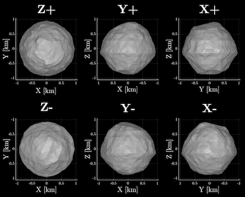
The MLA has delivered more than 40 million measurements of the shape of Mercury at about 26 million individual footprint locations. These locations are focused around the North Pole, with 78.5% of all measurements located between 50° N and 84° N. The topography at the footprint location is determined from the position of the spacecraft, the orientation of the instrument, and the measured range to the surface.


Previously, two methods have been proposed for the retrieval of tidal surface displacements from laser altimetry data: The crossover method (e.g., Mazarico et al., 2014) and a global approach, which simultaneously solves for global topography and h2 (Thor et al., 2020). In the global approach, the topography is parametrized as an expansion in 2D cubic B-splines on an equirectangular grid with resolutions reaching up to 32 grid cells per degree.


Here, we investigate the possibility to substitute the solution for topography in the global approach by the usage of a prescribed topographic model. This so-called direct altimetry approach has not been applied to the problem of retrieving tides from laser altimetry yet. We use a high-resolution (64 pix / degree) digital terrain model (DTM) obtained by photogrammetric evaluation of images obtained by the Mercury Dual Imaging System (MDIS, Becker et al., 2016) and compare the MLA topographic values to the corresponding values at the MLA measurement locations interpolated from the MDIS DTM.


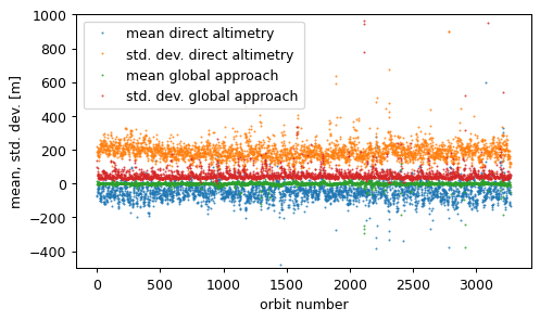
Figure 1: Mean and standard deviation of the residuals of the MLA measurements of each MESSENGER orbit, with respect to the MDIS data (direct altimetry approach) and to the topographic model obtained from the fit (global approach), respectively.


Fig. 1 shows the statistics of residuals between MLA topographic values and interpolated MDIS DTM values as well as the residuals of the adjustment applied in the global approach with a resolution of 16 grid cells per degree, equivalent to 2.7 km at the equator. The standard deviations over the entire data set are 83.59 m for the global approach and 251.06 m for the direct altimetry, respectively.


First, we note that for several orbits mean and standard deviation significantly exceed the usual levels. For both methods a careful elimination of outliers is indispensable. Outliers can be found in the MLA data per orbit and at individual measurements. The former type is likely related to the orbit determination process. Second, we note that even though the resolution of the DTM is at 64 pix / degree four times larger than the shown resolution of 16 grid cells per degree for the topographic model obtained in the global fit, its effective resolution is lower, leading to higher residuals. This shows that the photogrammetric DTM of Becker et al. (2016) has a worse fit to the MLA data than a coarser model derived from the MLA data itself. Therefore, the retrieval of the tidal signal from the photogrammetric DTM is challenging.


Future application of updated DTMs (Preusker et al. 2017) could remedy the low effective resolution when globally available. Furthermore, the co-registration of the MLA measurements to the DTM might lead to a better fit. However, this procedure comes with the concern that the stereo-photogrammetric generation of DTMs neglects tidal deformations.


References

Steinbrügge, G., Padovan, S., Hussmann, H., Steinke, T., Stark, A., & Oberst, J. (2018). Journal of Geophysical Research: Planets, 123, 2760– 2772.

Mazarico, E., Barker, M. K., Neumann, G. A., Zuber, M. T., and Smith, D. E. (2014), Geophys. Res. Lett., 41, 2282– 2288

Thor, R. N., Kallenbach, R., Christensen, U. R., Stark, A., Steinbrügge, G., Di Ruscio, A., ... & Oberst, J. (2020). Astronomy & Astrophysics, 633, A85.

Becker, K. J., Robinson, M. S., Becker, T. L., Weller, L. A., Edmundson, K. L., Neumann, G. A., ... & Solomon, S. C. (2016). In Lunar and planetary science conference (Vol. 47, p. 2959).

Preusker, F., Stark, A., Oberst, J., Matz, K. D., Gwinner, K., Roatsch, T., & Watters, T. R. (2017). Planetary and Space Science, 142, 26-37.

How to cite: Thor, R. and Stenzel, O.: Towards the extraction of the tidal signal from MESSENGER MLA data, Europlanet Science Congress 2020, online, 21 Sep–9 Oct 2020, EPSC2020-215, https://doi.org/10.5194/epsc2020-215, 2020.

EPSC2020-754ECP
William Desprats, Daniel Arnold, Michel Blanc, Stefano Bertone, Adrian Jäggi, Li Mingtao, Li Lei, and Olivier Witasse

Abstract

The gravity field of Callisto can be inferred using radio tracking data from a low-altitude orbiter around the icy moon. Orbit possibilities around Callisto are currently under study for the Gan De mission proposal [2]. However, gravity field recovery using Doppler observations is highly dependent on the orbit geometry. In this study, we will show the effect of different orbit constraints on the recoverability of Callisto’s gravity field parameters.

1. Introduction

The exploration of Callisto is part of the extensive interest in the icy moons characterization. In comparison to the other Galilean moons, Callisto has kept the best-preserved records of the Jovian system formation. As other missions will focus on Ganymede and Europa, mission proposals devoted to the exploration and characterization of Callisto are currently emerging [2][6].

The Gan De mission [2] is at a very early planning stage. Led by the National Space Science Center (NSSC), Chinese Academy of Science (CAS), this mission aims to send an orbiter around Callisto in order to characterize its surface and interior. Its degree of differentiation will also be investigated as well as the possible existence of an internal ocean, as Galileo measurements suggested.

As part of a global characterization of Callisto, the recovery of gravity field parameters is highly dependent on the orbital characteristics of the mission. In this presentation, we will analyze the impact of the orbit choice for an orbiter around Callisto.

2. Exploring different orbits

Multiple flybys of Callisto are expected from the JUICE and the Europa Clipper missions [5]. Even if this will provide additional information on Callisto, the global mapping of the outermost Galilean moon will be uniquely improved by means of an orbiter from a high inclination and a low altitude. A specific difficulty in the orbit design in the Jovian system is related to the orbit stability, which is highly impacted by the influence of Jupiter as a third body exerting strong perturbations on a Callisto orbiter Another constraint is to maximize the illumination by the Sun for solar power, which is of importance especially for low-altitude probes in the outer solar system. These constraints will all have direct implications on the orbit parameters.

In this presentation, we will select a number of different low Callisto orbits for Gan De, respecting different of the above mentioned constraints, and analyze and compare their scientific value for gravity field recovery. We will explore different altitudes, Sun beta angles, Earth beta angles and mission durations. We will also analyze the possibility to use repetitive ground track orbits [3].

3. Gravity field recovery simulation

Using an extended force model, different reference orbits will be propagated in the planetary extension of the Bernese GNSS Software (BSW) [4]. Today, our knowledge of Callisto’s gravity field is restricted to the results of the Galileo mission, which provided resulting its coefficients up to degree 2 coefficients [1]. In this presentation we will make use of a synthetic gravity field as ground truth for our simulation. Realistic Doppler tracking data (2-way X-band Doppler range rate) will be simulated as measurements from the Deep Space Network. These observations will then be used to reconstruct the orbit along with dynamical parameters. The focus of this presentation is on the quality of the retrieved gravity field parameters and tidal Love number k2.

Within this closed loop simulation, we will investigate the effect of the orbit geometry on the gravity field recovery. The effect of realistic tracking station schedule will also be considered, and an appropriate level of white noise will be added to synthetic Doppler observations.

Acknowledgements

This study has been funded with the support of the Swiss National Foundation (SNF).

References

[1] Anderson, J. D., et al. "Shape, mean radius, gravity field, and interior structure of Callisto." Icarus 153.1 (2001): 157-161.

[2] Blanc, M. et al: Gan De: Science Objectives and Mission Scenarios for China’s Mission to the Jupiter System, EGU General Assembly 2020, Online, 4–8 May 2020, EGU2020-20179.

[3] Cinelli, Marco, Christian Circi, and Emiliano Ortore. "Polynomial equations for science orbits around Europa." Celestial Mechanics and Dynamical Astronomy 122.3 (2015): 199-212.

[4] Dach, R. et al. "Bernese GNSS software version 5.2." (2015).

[5] Parisi, M. et al: "The gravity fields of Ganymede, Callisto and Europa: How well can JUICE do." Geophys. Res. Abstr. EGU2014 11758 (2014).

[6] Smith, D. E., et al. "MAGIC, A Discovery Proposal to the Icy Moon Callisto." AGUFM 2019 (2019): P34C-03.


How to cite: Desprats, W., Arnold, D., Blanc, M., Bertone, S., Jäggi, A., Mingtao, L., Lei, L., and Witasse, O.: Influence of Low Callisto Orbit design on gravity field recovery, Europlanet Science Congress 2020, online, 21 Sep–9 Oct 2020, EPSC2020-754, https://doi.org/10.5194/epsc2020-754, 2020.

EPSC2020-863
Mikael Beuthe

1. Introduction

Isostasy explains why observed gravity anomalies are generally much weaker than what is expected from topography alone, and why planetary crusts can support high topography without breaking up [1]. The apparent simplicity of the concept – buoyant support of mountains by iceberg-like roots – is belied by the debate that has been going on for over a century about ‘equal mass’ and ‘equal pressure’ prescriptions [2]. Since these isostatic models only differ at the planetary scale, it has not caused a problem for the application of isostasy to Earth because of its division in tectonic plates (large-scale geoid anomalies due to mantle convection are another reason). By contrast, isostasy on icy moons and dwarf planets is immediately faced with the problem of defining correctly isostasy at the largest scales. For this purpose, new isostatic models based on the minimization of stress [3], on time-dependent viscous evolution [4], and on stationary viscous flow [5] have recently been published (these models have historical precedents not cited here). The multiplicity of isostatic approaches is too much of a good thing. I will show that these new isostatic approaches are mostly equivalent.

2. Isostasy with Love

Isostasy can be formulated very generally as a loading problem using the ‘Isostasy with Love’ approach sketched in [3]. In Airy isostasy, the shell is loaded by a surface load (‘L’) and a bottom load (‘I’ for internal). The bottom-to-surface loading ratio ζn depends on the harmonic degree n and must be determined with the chosen isostatic prescription.

In elastic isostasy (‘E ’), the bottom-to-surface shape ratio can be expressed in terms of radial Love numbers at the surface or bottom of the shell:

where the ‘hat’ denotes deviatoric Love numbers, defined by subtracting the fluid value from Love numbers.

In viscoelastic isostasy (‘V ’), the shape ratio is given by a very similar expression, except that the Love numbers (and possibly the load too) are now time-dependent:

For elastic isostasy, I consider here the model of Zero-Deflection Isostasy (ZDI), which is closely related to Minimum Stress Isostasy (MSI) but is simpler to formulate. In ZDI, the isostatic prescription states that the radial deflection vanishes at the surface (it could alternatively be zero at the bottom of the shell, but let us keep it simple). If the shell is homogeneous and the core is rigid, analytical formulas can be generated with the elastic propagator matrix method. For example, the topographic ratio (closely related to the shape ratio but taking the geoid into account [5]) is given by

where fn(x) is a degree-dependent function which is known in analytical form.

In viscoelastic isostasy, similar analytical formulas can be obtained, using the correspondence principle, for Visco-elastic Isostasy with constant Load (VeLI) and with constant surface Shape (VeSI). In the viscous approach, analytical formulas for Viscous Isostasy with constant Load (VLI) or constant Shape (VSI) can be obtained using the viscous propagator matrix approach.

3. Visco-Elastic equivalences

The comparison of analytical formulas for the shape ratio, topographic ratio, or compensation factor in elastic/viscoelastic/viscous isostasy demonstrates the equivalences shown in Figure 1. Isostatic models thus belong to two independent groups: the elastic/stationary approaches ZDI-VeSI-VSI (plus MSI, not discussed here), and the time-dependent approaches VeLI-VLI. In the thin shell limit, the two groups yield the same predictions as Thin Shell Isostasy (TSI) which was initially obtained through stress minimization in a thin shell [6]. At low harmonic degree, TSI is a good approximation for Europa but a bad one for Enceladus. At high harmonic degree, shell thickness always matters and the various models give slightly different predictions of geoid anomalies.

These equivalences hold beyond the simple analytical model based on a homogenous crust and a rigid core. The equivalence between ZDI and VSI can be understood in terms of the Stokes-Rayleigh analogy relating elastic and viscous solutions with analogous boundary conditions [7]. This equivalence extends to viscous models with depth-dependent viscosity [5], which correspond to elastic models with depth-dependent shear modulus. The equivalence between ZDI and VeSI can be proven using the correspondence principle and the invariance of elastic isostasy under a global rescaling of the shear modulus of the crust (the latter implies that ZDI can be computed in the fluid-crust limit). The equivalence between VSI and VeSI, on the one hand, and between VLI and VeLI, on the other, can be understood as due to memory loss of the initial elastic response.

In conclusion, the elastic, viscoelastic, and viscous approaches to isostasy are not that different. The focus should now be on choosing the right boundary conditions, which express different physical pictures. In particular, viscous/viscoelastic isostasy with a constant load represents a completely different loading history from viscous/viscoelastic isostasy with a constant surface shape maintained by a time-dependent load at the bottom of the shell.

Acknowledgements

This work was financially supported by the Belgian PRODEX program managed by the ESA in collaboration with the Belgian Federal Science Policy Office

References

[1] Melosh J. (2011), Planetary Surfaces Processes, CUP.

[2] Hemingway D.J. (2017), GRL 44, 7695.
[3] Beuthe M. et al. (2016), GRL 43, 10088.
[4] Ermakov A. et al. (2017), JGR 122, 2267.

[5] Cadek O. et al.(2019), GRL 46, 14299.

[6] Dahlen F.A. (1982), JGR 87, 3943.

[7] Ribe N. M. (2018), Theoretical Mantle Dynamics, CUP

How to cite: Beuthe, M.: Equivalence between elastic, viscoelastic, and viscous isostasy, Europlanet Science Congress 2020, online, 21 Sep–9 Oct 2020, EPSC2020-863, https://doi.org/10.5194/epsc2020-863, 2020.

EPSC2020-914ECP
Claire Marie Guimond, Oliver Shorttle, and John F. Rudge

Topography is a crucial component of the Earth system: having rock exposed to the atmosphere lets surface temperatures self-regulate via silicate weathering, for example. However, there are limits to a lithosphere’s capacity to support mountains or valleys over geologic time. We see in our solar system that the range in a body’s elevations tends to decrease with increasing planet mass. These trends, inherent to planetary building materials, are modelled using well-studied concepts from geodynamics. As a first step, we predict feasible thermal evolutions and dynamic topography scaling relationships for rocky planets, eventually gearing to ask how massive a planet can be and still likely maintain subaerial land.

How to cite: Guimond, C. M., Shorttle, O., and Rudge, J. F.: Does topography matter for rocky exoplanets?, Europlanet Science Congress 2020, online, 21 Sep–9 Oct 2020, EPSC2020-914, https://doi.org/10.5194/epsc2020-914, 2020.