Oral presentations and abstracts
Electromagnetic scattering phenomena play a key role in determining the properties of Solar System surfaces based on observations using different techniques and in a variety of wavelengths ranging from the ultraviolet to the radio. This session will promote a general advancement in the exploitation of observational and experimental techniques to characterize radiative transfer in complex particulate media. Abstracts are solicited on progresses in numerical methods to extract relevant information from imagery, photometry, polarimetry and spectroscopy in solid phase, reference laboratory databases, photometric modeling, interpreting features on planetary surfaces, mixing/unmixing methods… Software and web service applications are welcome.
Session assets
Introduction: The OSIRIS-REx mission has revealed a dark, boulder-rich, apparently dust-poor surface of the B-type asteroid (101955) Bennu [1], therefore a challenge for bi-directional reflectance (rF) modeling. With an estimated geometric albedo of 4.5% [2], Bennu is darker than many comets, and its reflectance distribution is dominated by single-scattering processes. The general approach to model a dark asteroid’s bi-directional reflectance distribution is to apply the standard Hapke IMSA model and its shadowing function [3]. However, this can imprecisely describe the roughness slopes for rocky surfaces [4]. Assuming that surfaces are fully diffuse can negate a specular forward-scattering contribution from crystalline components in the regolith [7]. To achieve a more complete photometric modeling of Bennu’s scattering curve, we rely on the radiative transfer semi-numerical model of Van Ginneken et al. [8,9].
Observations: MapCam is an optical imager [10] on-board the OSIRIS-REx spacecraft, equipped with four broadband color filters (60-90 nm wide) centered at 473 (b'), 550 (v'), 698 (w') and 847 (x') nm. We analyzed images acquired during the Equatorial Station (EQ), a campaign of the Detailed Survey mission phase [11], over a full rotation of (101955) Bennu at a nadir spatial resolution of ~33 cm/px. EQ comprehended seven phase angle configurations α =[7.5° ,30° ,45° ,90° ,130°] .
We analyzed the pixel subtended by the mission’s candidate sample collection sites, for which highly precise, laser altimeter-based digital terrain models (DTMs) were available [12,13]. These four candidate sites were called Sandpiper (latitude=-47°; longitude=322°), Osprey (11°; 88°), Nightingale ( 56°; 43°), and Kingfisher (11°; 56°). The varied latitude and longitudes provided the range of observational conditions required for our analysis.
Methodology: The methodology consists of the following steps:
a) NAIF SPICE kernels [14] and the DTMs are ingested into a ray-tracing code for rendering shadowed images. This allows us to discount for the effects of macroscopic shadows, leaving only the sub-facet texture to be modeled. These ancillary images provide the incidence, emergence, phase & azimuth for every facet.
b) We apply Van Ginneken’s model to every facet. Occlusion and shadowing as well as the retro-reflection among the reliefs are taken into account. The model has two major components: the analytical expression for the specular reflection; and the numerically-integrated diffusive reflection. At total, the model has three free parameters: ρ (single-scattering albedo), σ (RMS roughness slope), and g (specular-to-diffuse ratio), plus the three more related to the scattering phase function (bi-lobe Henyey-Greenstein function: c, b1, and b2)
c) Inverse problem: We run the Monte Carlo Markov Chain to sample the multi-parametric space in order to reconstruct a posteriori probability distribution of solutions for every free parameter, i.e., (ρ, σ, g, b1, b2, c), from which the statistics for every solution are estimated.
Results: The MCMC technique reveals some interesting aspects of Bennu's surface (Fig. 1): while the RMS roughness slope of 27+1-5 is in line with what has been obtained for other asteroids using Hapke shadowing function, we are puzzled by the indication of a non-zero specular reflection ratio from the surface (2.6+1−0.8 %). The specular reflection hints at a possible mono-crystalline component.
As for the diffuse rough component, the analysis of the photometric correction of OCAMS images taken at varied phase angles (α) indicates a more complex scenario. Up to α = 90°, the photometric correction is vastly improved by mixing two different solutions for roughness (one with low RMS σ and another with global RMS σ), a bi-modality already perceived from the MCMC a posteriori distributions. We have shown that most of Bennu's brightness variation can be explained by tuning the roughness slope statistical distribution.
Finally, we report a back-scatter phase function for the phase angle range between 7.5°, and 130°, without any expressive spectral trend in the visible range. The MCMC inversion hints at a possible second forward-scatter lobe of at least ~0.2 width. This leads to two possible solutions for the asymmetric factor (ξ (1) = −0.360 ± 0.030 and ξ(2) = −0.444 ± 0.020). We also report a dark global approximate single-scattering albedo at 550 nm from the collective analysis of all site candidates of 4.64+0.08-0.09 % . The single-scattering MapCam four-band colors show a similar spectral trend to the global average OVIRS EQ3 spectrum. The four sites together provide a general description of Bennu's colors.
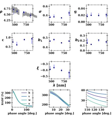
Fig. 1. Parametric solutions after the MCMC technique for all sample sites together, and the scattering phase function (bottom row) for each MapCam filters.
References:
[1] Lauretta, D. et al. Met.. & Plan. Scie., 50, Issue 4, 834-849, 2015.
[2] DellaGiustina, D.N. et al., Nat. Astron. 3, 241-351, 2019.
[3] Hapke, B. Icarus 59, 41-59,1984.
[4] Shkuratov et al., JQSRT 113, 18, 2431-2456, 2012.
[5] Davidsson, B. et al. Icarus 201, 335–357, 2009.
[6] Labarre, S. et al. Icarus 290, 63-80, 2017.
[7] Bowell, E., et al. Asteroid II, Univ. of Ariz. Press, 1989.
[8] Van Ginneken, B. et al. AO 37, 130-139, 1998.
[9] Goguen, J. et al. Icarus 208, 548–557, 2010.
[10] Rizk, B. et al.. Space Sci. Rev. 214, 26, 2018.
[11] DellaGiustina, D.N. et al., ESS 5, 929, 2018.
[12] Daly, M. G. et al., SSR 212, 899, 2017.
[13] Barnouin, O. S. et al., PLANSS 180, 104764, 2020.
[14] Acton, C. H.. PLANSS 44.1 (1996): 65-70.
[15] Hapke, B. Cambridge Univ. Press, 2ed., 2012.
How to cite: Hasselmann, P. H., Fornasier, S., Barucci, M. A., Praet, A., Clark, B. E., Li, J.-Y., Golish, D., N. DellaGiustina, D., Deshapriya, P., Zou, X.-D., G. Daly, M., S. Barnouin, O., A. Simon, A., and S. Lauretta, D.: Modeling first-order scattering processes from OSIRIS-REx color images of the rough surface of asteroid (101955) Bennu, Europlanet Science Congress 2020, online, 21 Sep–9 Oct 2020, EPSC2020-122, https://doi.org/10.5194/epsc2020-122, 2020.
OVIRS [1, 2] acquired visible to near-infrared spectra of asteroid Bennu’s surface showing an asymmetric absorption band centered at 2.74 ± 0.01 μm [3], attributed to the presence of hydrated phyllosilicates. This feature is widespread across Bennu’s surface. Such an absorption band has been detected in some carbonaceous chondrite meteorites [4, 5].
In this study, we report the results from two distinct methods to estimate the hydration of Bennu’s surface. We calculated the normalized optical path length (NOPL) as well as the effective single particle absorption thickness (ESPAT) [6, 7, 8] on Bennu’s hydration band and on the selected meteorite spectra. For both methods, we compare meteorite results with their H2O/OH– H content, to estimate a H2O/OH– H content of Bennu’s average surface. Carbonaceous chondrite meteorite H2O/OH– H contents are derived from laboratory studies [9, 10].
Bennu spectra. Analysed spectra were acquired by OVIRS during Equatorial Station 3 (EQ3) of the Detailed Survey mission phase, on May 9, 2019, at 12:30 pm local solar time [11]. The reflectance spectra have been calibrated and photometrically corrected to an incidence angle of 0°, emission angle of 30°, and phase angle of 30°, using a McEwen photometrical model [12].
Meteorite spectra. We used three sets of meteorite absolute reflectance spectra, from [4,5], [8], and [13]. For each set, powdered meteorite sample spectra were measured under vacuum (asteroid-like conditions).
We selected over 40 meteorites for which bulk H values have been independently measured [9, 10]. In the case of Orgueil, Bells, and Tagish Lake, several samples were analysed and several H contents were ultimately derived [9, 14], all of which were used.
Normalized Optical Path Length (NOPL). The NOPL parameter was calculated as described in [6, 7, 8] on each meteorite spectrum, each individual Bennu reflectance spectrum, and the global average spectrum of Bennu. A linear continuum was fitted from 2.67 to 3.3 μm. The wavelength, at which the NOPL parameter is calculated, is the mean band minimum position for the EQ3 data set at 2.73 μm. Methods used to locate the band minimum are described in [3].
Effective Single Particle Absorption Thickness (ESPAT). The ESPAT parameter was calculated following the method of [6, 7, 8]. Absolute reflectance spectra of meteorites and Bennu’s surface were first converted into single-scattering albedo spectra [6, 7, 8]. A linear continuum was then fitted from 2.67 to 3.3 μm and the ESPAT parameter is calculated at 2.73 μm as well. Our analyses do not include the organic absorption bands, present longwards of ~3.3 μm [11, 15]. Thus, we compare NOPL and ESPAT results with the hydrogen content of H2O/OH– groups in hydrated phyllosilicates only, measured for the selected meteorites [9, 10].
Figure 1 shows the NOPL parameter variations across Bennu’s surface using EQ3 spectra.
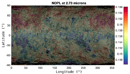
Figure 1: Map of NOPL values computed at 2.73 μm for each EQ3 spectrum of Bennu.
We find a linear correlation (Figure 2) between the NOPL parameter calculated at 2.73 μm on meteorite spectra and the meteorite H2O/OH– H content.
Using this linear correlation, for the NOPL calculated on Bennu’s EQ3 average spectrum, we estimate a H2O/OH– H content for Bennu’s average surface of 0.54 ± 0.11 wt.%.

Figure 2: Linear correlation between NOPL calculated at 2.73 μm and H2O/OH– H content of the seven selected meteorites (in colored points), and for average Bennu (blue circle).
As with the NOPL parameter, we also find a linear correlation between the ESPAT parameter calculated at 2.73 μm on meteorite spectra and the meteorite H2O/OH– H content. We therefore estimate a H2O/OH– H content for Bennu’s average surface of 0.49 ± 0.13 wt.%, using Bennu’s EQ3 mean ESPAT value and the latter correlation.
Discussion and Conclusion
The H2O/OH– H content for Bennu’s average surface obtained using NOPL parameters is consistent with the range obtained with the ESPAT parameter. Both methods are based on estimating global H content (in H2O/OH– groups of hydrated phyllosilicates) by analogy with meteorite data. The values of H2O/OH– H content of Bennu’s average surface we obtained are 0.54 ± 0.11 and 0.49 ± 0.13 wt.% using the NOPL parameter and the ESPAT parameter, respectively. From our results (Figure 2), Bennu’s average surface is most similar to heated CMs and Tagish Lake. Both estimated H2O/OH– H content ranges of Bennu’s average surface are more consistent with those of CM meteorites (0.46–1.36 wt%), Tagish Lake (0.50–0.69 wt.%), CR meteorites (0.30–1.20 wt.%), and CO meteorites (0.49–0.52 wt.%) [3, 9]. The gaussian modeling of the hydration band will complete those results.
Acknowledgements
This material is based on work supported by NASA under Contract NNM10AA11C issued through the New Frontiers Program. AP, MAB, FM, SF, PH and JDPD acknowledge funding support by CNES. INAF participation was supported by Italian Space Agency grant agreement n. 2017-37-H.0. We are grateful to the entire OSIRIS-REx Team for making the encounter with Bennu possible.
References
[1] Lauretta D. S. et al. (2017) Space Sci. Rev. 212, 925-984. [2] Reuter D. C. et al. (2018) Space Sci. Rev. 214, 54. [3] Hamilton V. E. et al. (2019) Nat. Astron. 3, 332. [4] Takir D. et al. (2013) Meteorit. Planet. Sci. 48, 1618–1637. [5] Takir D. et al. (2019) Icarus 333, 243–251. [6] Milliken R. E. et Mustard J. F. (2005) JGR, 110, E12001. [7] Milliken R. E. et al. (2007) JGR, 112, E08S07. [8] Garenne A. et al. (2016) Icarus, 264, 172-183. [9] Alexander C.M.O’D. et al. (2012) Science, 337, 721-723. [10] Alexander C.M.O’D. et al. (2013) Geochim. Cosmochim. Acta, 123, 244-260. [11] Simon et al. (in revision) Science. [12] Zou X.-D. et al., this meeting. [13] Potin S. et al. (2020) Icarus, 348, 113826. [14] Gilmour C. M. et al. (2019) Meteorit. Planet. Sci. 54, 1951–1972. [15] Kaplan et al. (2020) LPSC LI, 1050.
How to cite: Praet, A., Barucci, A., Kaplan, H., Merlin, F., Clark, B., Simon, A., Hamilton, V., Emery, J., Howell, E., Lim, L., Zou, X.-D., Reuter, D., Ferrone, S., Deshapriya, P., Fornasier, S., Hasselmann, P., Poggiali, G., Brucato, J., Takir, D., and Lauretta, D.: Hydration variations of Bennu’s surface: comparison of different methods. , Europlanet Science Congress 2020, online, 21 Sep–9 Oct 2020, EPSC2020-136, https://doi.org/10.5194/epsc2020-136, 2020.
1.Introduction
NASA’s OSIRIS-REx (Origins, Spectral Interpretations, Resource Identification, and Security–Regolith Explorer) asteroid sample return mission (Lauretta et al., 2017) began operating in proximity to near-Earth asteroid (101955) Bennu in December 2018. Here we present an analysis of the global photometry of Bennu from measurements by the OSIRIS-REx Visible and InfraRed Spectrometer (OVIRS; Reuter et al., 2018). This instrument is a point spectrometer with a wedged filter design. OVIRS is used for the spectral characterization of the surface of Bennu, with a field of view of 4 mrad and an effective spectral range from 0.4 to 4.3 μm. Our work focuses on OVIRS data acquired from December 9, 2018, to September 26, 2019.
2.Dataset
This study comprises the global observation data from Preliminary Survey and the two sub-phases of Detailed Survey, Baseball Diamond (BBD) and Equatorial Stations (EQ) (campaigns described in Lauretta et al., 2017). We use a total of 299,702 calibrated spots. More details about the data selection and calibration are introduced by Zou et al. (submitted).
3.Photometric analyses
We model the scattering properties of the surface of Bennu using the Lommel-Seeliger, Minnaert, McEwen, and Akimov photometric models. The best-fit model is a McEwen model with an exponential phase function and an exponential polynomial partition function. We use this model to correct the OVIRS spectra of Bennu to a standard reference viewing and illumination geometry at visible to infrared wavelengths for the purposes of global spectral mapping (Figure 1). We derive a bolometric Bond albedo map in which Bennu’s surface values range from 0.021 to 0.027. We find a phase reddening effect of 1.4±0.3 × 10⁻⁴ μm−1deg−1 across the wavelength range 0.48 to 2.5 μm, and our model is effective at removing this phase reddening.
We compare our OVIRS results to Golish et al. (2020)’s report on the global photometry of Bennu, based on imaging data from the OSIRIS-REx Camera Suite (OCAMS; Rizk et al., 2018). We also compare the results to ground observation and other minor planets including Ryugu.
Acknowledgements: This material is based upon work supported by NASA under Contract NNM10AA11C issued through the New Frontiers Program. We are grateful to the entire OSIRIS-REx Team for making the encounter with Bennu possible and the exploration highly successful. X.-D. Zou and J.-Y. Li also acknowledge partial support from the Solar System Exploration Research Virtual Institute 2016 (SSERVI16) Cooperative Agreement (Grant NNH16ZDA001N), SSERVI-TREX to the Planetary Science Institute. M. A. Barucci acknowledges funding support from CNES.
References
Bennett, C.A., et al. 2020. A high-resolution global basemap of (101955) Bennu. Icarus. doi: 10.1016/j.icarus.2020.113690.
Ernst et al., 2018, The Small Body Mapping Tool (SBMT) for Accessing, Visualizing, and Analyzing Spacecraft Data in Three Dimensions, LPSC 49, abstract no. 1043.
Golish, D.R., et al. 2020. Disk-resolved photometric modeling and properties of asteroid (101955) Bennu. Icarus, doi:10.1016/j.icarus.2020.113724.
Lauretta, D.S., et al. 2017. OSIRIS-REx: sample return from asteroid (101955) Bennu. Space Science Reviews 212(1-2):925-984.
Reuter, D.C., et al. 2018. The OSIRIS-REx Visible and InfraRed Spectrometer (OVIRS): spectral maps of the asteroid Bennu. Space Science Reviews 214(2):54.
Rizk, B., et al. 2018. OCAMS: the OSIRIS-REx Camera Suite. Space Science Reviews 214(1):26.
Zou et al. (submitted). Photometry of asteroid (101955) Bennu with OVIRS on OSIRIS-REx. Icarus.
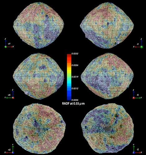
Figure 1. A global 3D facet-based map of the photometrically corrected (to 30°, 0°, 30°) OVIRS spots at a wavelength of 0.55 μm. The data are overlain on the OCAMS imaging basemap (Bennett et al., 2020), as viewed in the Small Body Mapping Tool (Ernst et al. 2018). Input spectra were obtained during Detailed Survey EQ3.
How to cite: Zou, X.-D., Li, J.-Y., Clark, B., Golish, D., Ferrone, S., Simon, A., Reuter, D., Domingue, D., Kaplan, H., Barucci, M., Fornasier, S., Praet, A., Hasselmann, P., Bennett, C., Cloutis, E., Tatsumi, E., DelllaGiustina, D., and Lauretta, D.: The Global Average Disk-Resolved Photometric Properties of (101955) Bennu, Europlanet Science Congress 2020, online, 21 Sep–9 Oct 2020, EPSC2020-146, https://doi.org/10.5194/epsc2020-146, 2020.
Introduction: Reflectance spectroscopy is commonly used to retrieve chemical and physical properties of the Solar System bodies. However, the reflectance spectrum of a surface depends not only on its composition, but also on several parameters, including the viewing geometry [1]. Unlike laboratory measurements where the composition and texture of the sample and the geometry of measurement are fixed and controlled, observations of planetary bodies integrate spatial heterogeneities and changes of observation geometries due to both the shape and the topography of the surface. Here we compare two spectral photometric models to reproduce laboratory measurements of the Bidirectional Reflectance Distribution Functions (BRDFs) of a sample. We then employ the resulting models to calculate phase curves of the dwarf planet Vesta at different wavelengths and simulate spectral image cubes of its surface acquired with virtual telescopes.
Laboratory measurements: Bidirectional reflectance spectroscopy of a fine powder of howardite is acquired using the spectro-gonio radiometer SHADOWS [2], using the geometrical configurations presented in [1].
Inversion models: Inverting photometric models consists in estimating the best values of their parameters to reproduce the BRDFs sampled in the laboratory. It is then possible to generate the reflectance spectra that would have been measured under any geometrical configuration needed for the planetary simulation. We consider two photometric models: the Hapke model based on physical principles and a modified version of the Ross-Thick Li-Sparse model [3]. The model is able to recreate BRDFs of many natural surfaces and was recently modified by [4] to increase its performances. We use the following RTLSR form:
R(θ,Ω,Φ,λ)=fiso(λ)+fvol(λ)Kvol(θ,Ω,Φ)+fgeo(λ)Kgeo(θ,Ω,Φ)+ffwd(λ)Kvol(θ,Ω,Φ)
where the K terms play the roles of Lambertian (iso), volumetric (vol), geometric (geo), and forward scattering (fwd) components respectively. Spectral weights fiso , fvol , fgeo, and ffwd of the four components are determined by the surface reflectance properties. Note that the volumetric kernel contains a simplified treatment of the opposition effect with fixed width and amplitude as this effect is poorly constrained by our measurements. As for the inversion of the models, we consider a Bayesian framework using either a sampling approach based on Markov Chain Monte Carlo [5] or an inverse regression approach based on a preliminary learning step [6,7].
Results and comparison of the models: Both models, Hapke and RTLSR, accurately recreate the spectral features observed on the measurements (fig. 1)
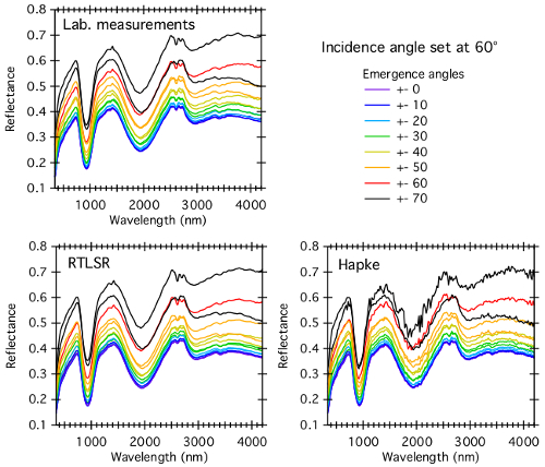
Fig. 1: Bidirectional reflectance spectroscopy of the howardite measured in the laboratory (top left panel), and simulations based on inversion with the RTLSR model (bottom left panel) and with the Hapke model (bottom right model).
It has been shown previously [8] that the Hapke model can have difficulties when modeling the reflectance of chips that cannot be considered as loose agglomerates of grains. The parametric formulation of the RTLSR model can be a more robust descriptor of the BRDF but offers very limited physical interpretation. The sample of howardite used here consists of a fine powder with a narrow grain size distribution, thus the results found here are similar between the two models. We will thereafter use the RTLSR model, which has a slightly better SNR.
Application to surface: We then applied the RTLSR spectral BRDF on each facet of a shape model of Vesta. We create a simulated Vesta covered with the fine powder of howardite over the whole surface. We then simulate a serie of images taken during the fly-by of a spacecraft near this simulated object, with a fixed illumination source and a range of phase angle from 6° to 135°. Along with the varying phase angle due to the fly-by, the shape of the body and its surface topography induce local variations of the geometrical configuration (fig. 2), thus creating variations in the reflectance spectra.
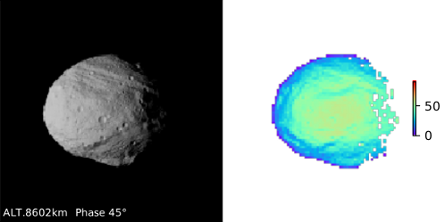
Fig. 2: Left: Radiance image of Vesta at 400nm as observed with a representative imaging spectrometer. Right: Local emergence angles measured on each facet of the shape model of Vesta.
In the case of an unresolved observation, the reflectance spectrum of a body is integrated over its whole surface, thus averaging the reflectance at fixed phase angle over all geometrical variations due to the shape and topography. We then compare various spectroscopic and photometric phase curves of the simulated Vesta and the howardite sample measured in the laboratory as exemplified in fig. 3.
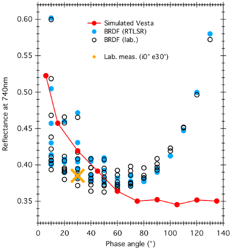
Fig. 3: Photometric phase curve of the simulated Vesta integrated over the whole surface (red solid line) compared to the BRDFs values measured in the laboratory (black circles) and inverted using the RTLSR model (blue circles).
The shape of the phase curve of the simulated Vesta shows a decreasing reflectance with increasing phase angle, typical of the micro and macroscale structures of the surface, drastically different from the phase curve measured in the laboratory. When comparing the spectroscopic parameters of the simulated Vesta to laboratory measurements acquired in the typical geometry of i0° e30°, we show that in the laboratory the reflectance is underestimated, while the spectral slope and amplitude of the absorption features are overestimated. As the composition of the surface of the simulated body is fully homogeneous, these differences are only due to the shape and topography of the asteroid.
Conclusion: We show here and application of a laboratory measured BRDF for the simulation of spectral image cubes and phase curves of a planetary body. If the observed body is not fully resolved, as it is often the case for asteroids spectroscopy, the measured reflectance spectrum is averaged over the whole surface. The observed spectra can be different from those measured in the laboratory, only because of geometrical effects due to the shape and topography of the surface.
References: [1] S. Potin et al. (2019) Icarus, 333, 415-428. [2] S. Potin et al. (2018) Applied Optics, 57, 8279-8296. [3] W. Lucht et al. (2000), IEEE Trans. Geosci. Remote Sens., 38, 977-998. [4] Z. Jiao et al. (2019) Remote Sens. Env., 221, 198-209. [5] F. Schmidt et al. (2015), Icarus, 260, 73-93. [6] A. Deleforge et al. (2014), Stat. & Comp. [7] B. Kugler et al. (2020), this conference [8] S. Potin et al. (2020), 51th LPSC, 1874.
How to cite: Potin, S., Douté, S., Kugler, B., Forbes, F., Beck, P., and Schmitt, B.: Simulated phase curves of Vesta based on laboratory bidirectional reflectance spectroscopy, Europlanet Science Congress 2020, online, 21 Sep–9 Oct 2020, EPSC2020-201, https://doi.org/10.5194/epsc2020-201, 2020.
Recent numerical simulations (Greenstreet et al. 2012, Granvik et al. 2018) predicted the existence of a population of small bodies that is orbiting entirely inside Venus orbit. They could represent about 0.22 % of the steady-state near-Earth asteroids (NEAs). These asteroids are called Vatiras (by analog with the Atira-class NEAs) or Interior to Venus Orbit Objects. However, only at the beginning of this year (January 4, 2020) the first one was discovered by Zwicky Transient Facility (Bolin et al. 2020). It is called 2020 AV2 and has the aphelion at 0.654 AU, and the perihelion at 0.457 AU.
The dynamical history of this object has been explored using N-body simulations (de la Fuente Marcos & de la Fuente Marcos 2020). It has been shown that 2020 AV2 was a former Atira-class, and perhaps a former Aten-class asteroid, which reached the Vatira orbit relatively recently in astronomical terms, ∼105 yr (within 9σ confidence level). Similar results have also been reported by Greenstreet (2020).
The orbit of 2020 AV2 makes it a peculiar case compared with those of the near-Earth asteroids. It is subjected to high temperature, strong solar wind irradiation, and close approaches to Mercury and (more distant) Venus. In this context, we carried out an observing run aimed at obtaining spectroscopic and photometric data for 2020 AV2. We used the 2.56 m Nordic Optical Telescope (NOT) and 4.2m William Herschel Telescope (WHT), both located at El Roque de los Muchachos Observatory in La Palma, Canary Islands (Spain). The observations were performed on the evenings of January 11, 13, and 14, 2020. They were challenging due to the low maximum elongation of this target (about 37 deg during our observations).
We obtained two visible spectra with the ACAM/WHT and with the ALFOSC/NOT instruments. The near-infrared part of the spectrum was obtained with the LIRIS/WHT instrument using the lr-zj prism. It covers the 0.9-1.5 μm wavelength range. The merged spectrum is shown in Fig. 1.

Fig.1 The combined visible - near infrared spectrum of 2020 AV2 (Popescu et al. 2020). The spectral curve is normalized to unity at 1.25 μm. The reflectance maximum at 0.745 μm and the band minimum at 1.075 μm are outlined by the two markers.
The merged spectrum, covering a wavelength interval between 0.5 and 1.5 μm, allowed us to classify 2020 AV2 as an Sa-type asteroid. The value estimated for the 1 μm band center, BIC = 1.08 ± 0.020 μm, points towards a composition similar to that of the S(I) subtype of asteroids with olivine-pyroxene mixtures, defined by Gaffey et al. (1993). This value of BIC is indicative of a ferroan olivine mineralogy similar to that of brachinite meteorites.
Last but no least, we derived the effective diameter of this Vatira to be 1.50+1.10−0.65 km by considering the average albedo of A-type and S-complex asteroids (pV = 0.23−0.08+0.11), and the absolute magnitude (H=16.40 ± 0.78 mag).
References: [1] Bolin et al. 2020, MPEC 2020-A99; [2] de la Fuente Marcos & de la Fuente Marcos, 2020, MNRAS, 494, L6; [3] Granvik et al. 2018, Icarus, 312, 181; [4] Greenstreet et al. 2012, Icarus, 217, 355; [5] Greenstreet 2020, MNRAS, 493, L129; [6] Popescu et al. 2020, MNRAS, paper accepted, https://doi.org/10.1093/mnras/staa1728
Acknowledgements: This work was developed in the framework of EURONEAR collaboration and of ESA P3NEOI projects. The work of M.P. was supported by a grant of the Romanian National Authority for Scientific Research - UEFISCDI, project number PN-III-P1-1.2-PCCDI-2017-0371. M.P., J.dL. and J.L. acknowledge support from the AYA2015-67772-R (MINECO, Spain), and from the European Union's Horizon 2020 research and innovation programme under grant agreement No 870403 (project NEOROCKS).This work was partially supported by the Spanish MINECO under grant ESP2017-87813-R. Based on observations made with the William Herschel Telescope (operated by the Isaac Newton Group of Telescopes) and the Nordic Optical Telescope. The paper make use of data published by the following web-sites Minor Planet Center, JPL Small-Body Database Browser , SMASS - Planetary Spectroscopy at MIT.
How to cite: Popescu, M., de León, J., de la Fuente Marcos, C., Văduvescu, O., de la Fuente Marcos, R., Licandro, J., Pinter, V., Tatsumi, E., and Curelaru, L.: Spectral properties of 2020 AV2, the first known asteroid orbiting inside Venus orbit, Europlanet Science Congress 2020, online, 21 Sep–9 Oct 2020, EPSC2020-549, https://doi.org/10.5194/epsc2020-549, 2020.
Linear least squares unmixing of infrared spectra is a fast and effective way to spectrally estimate the modal mineral abundances of laboratory samples and remotely-sensed surfaces to within 5% on average [e.g., 1]. This technique has been applied to spectra of whole rocks, coarse particulates, meteorites, and the Martian surface to successfully determine modal abundances [e.g., 1-3]. With the recent arrival of NASA’s OSIRIS-REx spacecraft to asteroid 101955 Bennu, the OSIRIS-REx Thermal Emission Spectrometer (OTES) has been providing a wealth of data to interpret using spectral unmixing techniques [e.g., 4].
The assumption of linear spectral unmixing allows for the deconvolution of a mixed spectrum if the individual spectra and particle sizes of the pure end members are present within a spectral library. By implementing a weighted linear least squares (WLS) unmixing algorithm, one is able to deconvolve these mixed spectra into areal percentages of each endmember with the underlying assumption that this then corresponds to the volume percentages [e.g., 1-3]. At thermal infrared (TIR) wavelengths, end member spectra of coarse particulates combine linearly due to high absorption coefficients and relatively small mean optical paths, which limits most of the volumetric scattering [e.g., 1-3]. Linearity in the TIR region continues as particle size decreases until the wavelength of light approaches the particle size, at this point particles become optically thin and non-linear behavior (e.g., volumetric scattering) is observed. However, Ramsey and Christensen [1] demonstrated that when unmixing fine particulates (10 – 20 μm) with a spectral library of end members at the same particle size linear unmixing can still be used to estimate modal mineral abundances.
In this study we investigate the effectiveness of a linear least squares unmixing approach to estimate mineral abundances for samples dominated by fine particulates (< 38 μm). We use a WLS algorithm and a spectral library of fine particulate pure minerals to unmix spectra of a suite of fine particulate, primitive asteroid analogs. Results from this investigation have implications for the interpretation of spectral observations of primitive asteroids that have a layer of fine particulate regolith.
[1] Ramsey M. S. and Christensen P. R. (1998) JGR, 103, 577-596. [2] Hamilton V. E. and Christensen P. R. (2000) JGR, 105, 9717-9733. [3] Rogers A. D. and Aharonson O. (2008) JGR, 113,EO6S14. [4] Hamilton V. E. et al. (2019) Nature Astron., 3, 332-340.
How to cite: Lowry, V., Donaldson Hanna, K., Campins, H., Bowles, N., and Hamilton, V.: Linear unmixing of fine particulate materials: implications for compositional analyses of primitive asteroids, Europlanet Science Congress 2020, online, 21 Sep–9 Oct 2020, EPSC2020-400, https://doi.org/10.5194/epsc2020-400, 2020.
Abstract:
As part of a larger study to elucidate the presence of hydrated minerals on asteroid surfaces, we are developing a robust taxonomic classification system using spectroscopic observations in the vicinity of 3 μm. We have constructed a Python algorithm to identify band centers and band depths near 3 µm for a set of normalized, thermally-corrected asteroid spectra for use to serve as inputs to Python’s Scikit-Learn library of Machine Learning (ML) algorithms. We anticipate a thorough investigation of both Principal Component Analysis and ML (supervised, unsupervised, and Artificial Neural Network) techniques to assess which technique is likely to be better suited for classifying the 3-µm data. At this writing, we have run tests using Python’s Agglomerative clustering ML algorithm to examine possible clustering scenarios. These initial steps have given us some familiarity with the mechanics of using ML on the 3-µm dataset as well as serving to identify some possible pitfalls or cul-de-sacs. Presented here are the preliminary results we have obtained.
Introduction:
Although various techniques have been used, asteroid classification has typically been done via Principal Component Analysis (PCA: [1,2]). PCA is a statistical technique that reduces the dimensionality of a dataset by identifying the most important parameters within a dataset based on their variance. Parameters that exhibit the greatest amount of variance are considered to be of greater importance while parameters with the least amount of variance are considered to be of lower importance. While the PCA technique produces better visualizations of the data by reducing the dimensionality of a dataset, the PCA technique comes with some drawbacks. Disadvantages such as its dependence on scale and information loss due to the orthogonal property of PCA can cause interpretation of PCA results to prove to be a more critical and time-consuming process. Therefore, exploring other means of classification may prove to be worthwhile.
Machine Learning (ML) algorithms have had a significant impact on the way in which data is analyzed and interpreted, and have already proven to be a powerfully reliable resource in the field of planetary science. Accordingly, the application of ML to an asteroid taxonomy has the potential to be more efficient, objective, and easy-to-implement than PCA. ML algorithms can be supervised, in which the program “learns” from training data and is able to classify new inputs, or unsupervised, in which the program analyzes the dataset to determine patterns such as clusters. [3] used an Artificial Neural Network (ANN, a subset of ML) to classify asteroids, work followed up by [4]. Recent explorations of supervised ML for asteroid taxonomy are promising, and have applied training sets from existing databases to new visible and/or NIR photometric data (e.g. [5,6,7]).
We seek to explore the benefits of ML algorithms, as well as compare and contrast to the PCA technique, in the production of an asteroid taxonomy. Our initial exploration has utilized a set of normalized, thermally-corrected asteroid spectra in the vicinity of 3 µm. We have identified band centers and band depths and served this parameter space as inputs to Python’s Agglomerative clustering ML algorithm.
Methodology:
Thermal corrections of the asteroid spectra were performed via a forward model that uses a modified version of the Standard Thermal Model (STM: [8]). The forward model treats the beaming parameter as a free parameter adjusting its value for each iteration of the STM until it converges onto a value that yields expected long-wavelength continuum behavior. Spectra were then normalized to unity at a wavelength of 2.3 µm, followed by identification of band centers and band depths near 3 µm using both polynomial and Gaussian fits. In addition, band depths were measured at wavelengths of 2.9 µm and 3.2 µm to gather more information on asteroid band shapes. Lastly, the aforementioned calculated spectral features were input into Python’s Agglomerative clustering algorithm to determine which asteroid spectra shared similar features.
Summary:
As part of a larger investigation to better understand hydrated mineralogies as they apply to asteroids, we have begun work towards developing a quantitative taxonomic framework derived from asteroid spectra in the wavelength range from 2.0-4.0 µm. Our exploration thus far of Python’s Agglomerative clustering algorithm has proven to be fruitful. Minor changes to the parameterization of this algorithm can yield very different results, which naturally can lead to different interpretations. The Agglomerative clustering algorithm is one of many the powerful ML algorithms we will explore against the PCA technique, all of which we will be discussing in our presentation.
References:
[1] Bus, S. J. and Binzel, R. P. (2002). Phase II of the Small Main-Belt Asteroid Spectroscopic Survey: A Feature-Based Taxonomy. Icarus, 158:146-177.
[2] DeMeo, F. E., Binzel, R. P., Slivan, S. M., and Bus, S. J. (2009). An extension of the Bus asteroid taxonomy into the near-infrared. Icarus, 202:160-180.
[3] Howell, E. S., Merenyi, E., and Lebofsky, L. A. (1994). Classification of asteroid spectra using a neural network. 99:10847-10865.
[4] Merenyi, E., Howell E. S., Rivkin A. S., and Lebofsky L. A. (1997). Prediction of water in asteroids from spectral data shortward of 3 µm. Icarus, 129:421-439.
[5] Moment, M., Trilling, D. E., Borth, D., Jedicke, R., Butler, N., Reyes-Ruiz, M., Pichardo, B., Peterson, E., Axelrod, T., and Moskovitz, N. (2016). First results from the rapid-response spectrophotometric characterization of near-earth objects using UKIRT. The Astronomical Journal, 151:98
[6] Popescu, Marcel & Licandro, Javier & Carvano, Jmf & Stoicescu, R. & De León, Julia & Morate, David & Boac\u{a, I.L. & Cristescu, C.. (2018). Taxonomic classification of asteroids based on MOVIS near-infrared colors. Astronomy & Astrophysics. 617. 10.1051/0004-6361/201833023.
[7] Wallace, S. M., Burbine, T. H., Sheldon, D., Dyar, M. D. (2019). Machine Learning applied to asteroid taxonomy based on reflectance spectroscopy: An objective method. LPSC 50, Abstract # 1097.
[8] Lebofsky, L. A., Sykes, M. V., Tedesco, E. F., Veeder, G. J., Matson, D. L., Brown, R. H., Gradie, J. C., Feierberg, M. A., Rudy, R. J. (1986). A refined standard thermal model for asteroids based on observations of 1 Ceres and 2 Palas. Icarus. 68:239-251.
How to cite: Richardson, M., Rivkin, A., and Sickafoose, A.: Investigating Machine Learning as a Basis for Asteroid Taxnomies in the 3-Micron Spectral Region, Europlanet Science Congress 2020, online, 21 Sep–9 Oct 2020, EPSC2020-963, https://doi.org/10.5194/epsc2020-963, 2020.
The SSHADE database infrastructure (http://www.sshade.eu) hosts spectral data of many different types of solids: ices, snows, minerals, carbonaceous matters, meteorites, IDPs and other cosmo-materials,… covering a wide range of wavelengths: from X-rays to millimeter wavelengths.
Its Search / Visualization / Export interface is open to the community since February 2018. It currently contains over 3500 spectra.
We are currently developping a 'band list' database that will provide the band parameters (position, width, intensity, isotopic species, attribution mode, ...) of a number of solids of astrophysical and planetary interest in various phases (crystalline, amorphous, ...) and mixtures (different compositions) and at different temperatures or pressures. We will first feed this database from critical compilations of all data published in various journals for pure ices and molecular solids (hydrates, clathrates, sulfur compounds, ...) and their mixture, including the own works of the members of the SSHADE consortium.
An efficient search tool will allow to filter on various parameters such as band position (or spectral range) and intensity, expected molecular or atomic formula, type of vibration (e.g. infrared, Raman, fluorescence...) and display the results graphically. A demonstrator prototype is online in the 'old GhoSST' database (https://ghosst.osug.fr/search/band).
This band list will be a key tool for astronomers and space explorers to identify unknown absorption bands observed in the spectra of the surface or atmosphere of many objects in the solar system. Once the best candidate solid selected by the user the tool will point to the best relevant spectral data present in the SSHADE databases.
How to cite: Schmitt, B., Bollard, P., Albert, D., Bonal, L., and Poch, O. and the SSHADE Consortium: SSHADE, its solid spectra databases and its future band list of molecular solids, Europlanet Science Congress 2020, online, 21 Sep–9 Oct 2020, EPSC2020-644, https://doi.org/10.5194/epsc2020-644, 2020.
Introduction
When studying the Martian surface, the composition of the materials is established on the basis of spectral detection, unmixing, and physical modelling using images produced by hyperspectral cameras. Information on the microtexture of surface materials such as grain size, shape, roughness and internal structure can also be used as tracers of geological processes (Fernando et al. PSS 2016). This information is accessible under certain conditions thanks to hyperspectral image sequences acquired over a site of interest from eleven different angles by the Compact Reconnaissance Imaging Spectrometer for Mars (CRISM@MRO, Murchie et al. JGR-Planets 2009) . Similar multi-angular observations can also be realized in the laboratory with spectro-photo-goniometers, on planetary analog materials or real extraterrestrial matter (Potin et al. Icarus 2019) . In both cases, the interpretation of the surface Bidirectional Reflectance Distribution Factor extracted from these observations, in terms of composition and microtexture, is based on the inversion of the Hapke model, a semi-empirical photometric model that relates physically meaningful parameters x to the reflectivity y of a granular material for a given geometry of illumination and viewing (Schmidt and Fernando Icarus 2015).
This work presents an efficient method, based on a learning approach in a Bayesian framework, able to invert the Hapke model on large experimental or remote sensing datasets, as illustrated on a challenging CRISM multi-angular sequence of images.
1 Inversion characteristics
In the CRISM case, the dataset provides both spatial and spectral dimensions. More specifically, each of the Nspatial spatial point of the scene is observed at Nspectral wavelengths, yielding Nspatial× Nspectral vectors of reflectance values. This high number of observations to be inverted usually makes approaches like Markov Chain Monte-Carlo simulations unacceptably slow. The approach we propose starts with a computer intensive learning phase that builds a statistical model for the Hapke model; it is then applied for all observables yobs.
Each observable is a vector of D reflectances, one for each geometry of measure. In the case of CRISM data, D = 11 is moderate, but in laboratory, D may be one order of magnitude higher. The statistical model we propose has the advantage to be able to handle high dimensional settings while remaining computationally tractable.
The Bayesian framework offers a natural solution to propagate uncertainties on measures, which are formalized as variance on the prior distribution, while the variance of the posterior distribution assesses the uncertainty induced by the inversion.
The complexity of the forward radiative transfer model often makes our inverse problem ill-posed. In practice, multiples solutions might be acceptable. More than a point estimator, our statistical model provides a full posterior density, whose multi-modality can be assessed and interpreted.
2 Bayesian inversion via a learning approach
From a statistical point of view, we formalize our model as couple of random variables (X,Y), where Y = F(X) + ε. X has a prior distribution on the physical parameters space, F is the forward model and ε is a centered Gaussian noise accounting for measure uncertainties. The main idea is to use a two steps approach: first, approximate this model by a parametric surrogate model, second use the surrogate model to invert the observations.
We chose the family of the so-called Gaussian Locally-Linear Mapping (GLLiM) (Deleforge et al StatComp 2015) . Such models are expressive enough to approximate highly non-linear, complex, forward models, while remaining tractable.
The learning step is performed by generating a training dictionary composed of samples from (X,Y), on which the likelihood is maximized by a standard EM algorithm. Regarding the dimensionality of the problem, the number of parameters is proportional to D, making this model suitable even for high dimensional observables. Moreover, the computational cost of the learning phase does not scale with the number of observations to be inverted.
The second step is performed by computing the posterior distribution of the random variable X given yobs. The inverse of the surrogate GLLiM has an explicit formulation in the form of a Gaussian Mixture. From this posterior density, the mean and variance are straightforward to compute. To handle a multi-solution scenario, the mixture can be further exploited.
3 Massive inversion of spectro-images
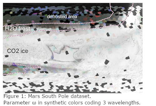
The dataset comes from a multi-angular observation of the South Pole of Mars by CRISM. The targeted scene presents spatially segregated C02 ice, H2O frost, and mineral dust (Douté and Pilorget EPSC 2017). After fusion and atmospheric correction of eleven hyperspectral images (Ceamanos et al. JGR-Planets 2013), the dataset provides both spatial and spectral dimensions, totaling Nobs = 154650 = 3093 × 50 measurements vectors yobs, which makes MCMC approach unacceptably slow. Maps of Hapke’s parameter values are generated from the results of our inversion and superposed with transparency onto the full resolution CRISM nadir image, which serves as a geological control background image.
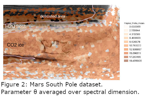
The results are satisfying from the application point of view. The colour composition of Figure 1 reflects the variation of ω at three wavelengths and corresponds well with the spatial distribution of the three previous materials and their known spectral optical properties. The map of the roughness parameter θ averaged over the spectral dimension (Figure 2) is color coded by intervals of values whose spatial variations are correlated with the composition and the structures of the terrains. In general, we find that all predicted parameters preserve some spatial regularity and show meaningful correlations with the composition and the geology.
Conclusion
We propose an efficient statistical and learning method for inverting physical models on massive remote sensing or experimental data. In the case of the Hapke model, the method has proved to produce satisfactory results for CRISM multi-angular acquisitions as illustrated in this paper and for laboratory spectrophotometric measurements as illustrated in Potin et al., this conference.
How to cite: Kugler, B., Forbes, F., and Douté, S.: An efficient Bayesian method for inverting physical models on massive planetary data, Europlanet Science Congress 2020, online, 21 Sep–9 Oct 2020, EPSC2020-335, https://doi.org/10.5194/epsc2020-335, 2020.
Abstract
One of the main difficulties to analyze modern spectroscopic datasets is the extremely large amount of data. For example, in atmospheric transmittance spectroscopy, the solar occultation channel (SO) of the NOMAD instrument onboard the ESA ExoMars2016 satellite called Trace Gas Orbiter (TGO) had produced ~10 millions of spectra in ~20000 acquisition sequences since the beginning of the mission in April 2018 until 15 January 2020. Usually, new lines are discovered after a long iterative process of model fitting and manual residual analysis.
Here we propose a new method, based on unsupervised machine learning, to automatically detect new minor species. Although precise quantification is out of scope, this tool can also be used to quickly summarize the dataset.
The methodology is the following: first we suggest to approximate the dataset by a linear mixture of abundance and endmember spectra. Then, unsupervised source separation is used, in form of non-negative matrix factorization. Several methods are tested on synthetic and simulation data.
On synthetic example, this approach is able to detect chemical compounds present at 1.5 times the noise level for 100 hidden spectra out of 104. Results on simulated spectra of NOMAD-SO targeting CH4 show a detection limit of 100 ppt in favorable conditions. Results on real martian data from NOMAD-SO show that CO2 and H2O are present, as expected, but CH4 is absent. Nevertheless, we find a set of new unexpected lines in the database.
Dataset
We propose here to focus on the Nadir and Occultation for MArs Discovery (NOMAD) instrument and especially the Solar Occultation (SO) channel [1], operating at wavenumbers from 2320 cm−1 to 4550 cm−1 (wavelength 2.2 to 4.3 μm).
Method
We propose to simplify the non-linear radiative transfer into a linear mixture. The collection of observation X is approximated by a few sources S and each of them present with an abundances A.
X=A.S (1)
Several algorithms have been proposed to solve this problem, subject to positivity (both S and A are non-negative). Such problem is called Non negative Matrix Factorization (NMF) [2]. This constraint is important to keep the physical meaning, but also to promote sparsity of S (a signal is sparse when a lot of values are close to zero except several non-zero values).
Results
Figure 1 and 2 present a synthetic toy example and demonstrate the capability of the method to extract a pure CH4 contribution, even hidden – 100 out of 10000 at 3-σ level of the noise.
Figure 3 illustrates the results on NOMAD data for order 136. Separated contribution of H2O and background are identified. No endmembers seemed to be related to CH4.
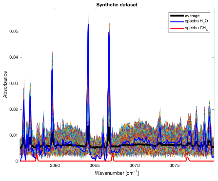
Figure 1: Synthetic dataset containing 104 spectra with various abundances of H2O and 100 containing CH4 at 3-σ level of the noise. In blue the reference spectra of H2O. In red the reference spectra of CH4.

Figure 2: Analysis of the dataset presented in figure 1 for NS = 4. Endmembers 1 and 3 are identified to the level with significant noise contribution, endmember 2 is identified to H2O, and endmember 4 is CH4.


Figure 3: (top) Results for real data of order 136 for NS = 5. The endmember 1 is identified to the level background (continuum misestimation), the endmembers 2, 3 and 4 are identified to H2O, either directly either from the adjacent orders. No endmember seems to be related to CH4. (bottom) Synthetic spectra from PSG [3]
Conclusion
We proposed a new machine learning tool [4], based on non-negative matrix factorization, to automatically detect new minor species. We applied it on potential CH4 detection on NOMAD-SO but future work should also focus on other order to allow new discovery by serendipity. Our tool may also be applied on other planetary spectral dataset, such as surface measurement.
Acknowledgements
We acknowledge support from the “Institut National des Sciences de l’Univers” (INSU), the "Centre National de la Recherche Scientifique" (CNRS) and "Centre National d’Etudes Spatiales" (CNES) through the "Programme National de Planétologie" and the ExoMars TGO programs. The NOMAD experiment is led by the Royal Belgian Institute for Space Aeronomy (BIRA-IASB), assisted by Co-PI teams from Spain (IAA-CSIC), Italy (INAF-IAPS), and the United Kingdom (Open University). This project acknowledges funding by the Belgian Science Policy Office (BELSPO), with the financial and contractual co-ordination by the ESA Prodex Office (PEA 4000103401, 4000121493), by Spanish Ministry of Science and Innovation (MCIU) and by European funds under grants PGC2018-101836-B-I00 and ESP2017-87143-R (MINECO/FEDER), as well as by UK Space Agency through grants ST/R005761/1, ST/P001262/1, ST/R001405/1 and ST/R001405/1 and Italian Space Agency through grant 2018-2-HH.0. This work was supported by the Belgian Fonds de la Recherche Scientifique - FNRS under grant number 30442502 (ET-HOME). The IAA/CSIC team acknowledges financial support from the State Agency for Research of the Spanish MCIU through the Center of Excellence Severo Ochoa award for the Instituto de Astrofísica de Andalucía (SEV-2017-0709).
References
[1] Vandaele et al., Space Science Reviews 214, 5, 2018
[2] Lee, D. D., Seung, H. S., 401, 788-791, Nature, 1999.
[3] Villanueva et al., 217, 86-104, JQSRT, 2018
[4] Schmidt et al., under review in JQSRT, 2020
How to cite: Schmidt, F., Cruz Mermy, G., Erwin, J., Robert, S., Neary, L., Thomas, I., Daerden, F., Ristic, B., Patel, M., Bellucci, G., Lopez-Moreno, J.-J., and Vandaele, A. C.: Machine learning for automatic identification of new minor species, Europlanet Science Congress 2020, online, 21 Sep–9 Oct 2020, EPSC2020-781, https://doi.org/10.5194/epsc2020-781, 2020.
Introduction:
Swirls are bright albedo features only found on the lunar surface. Almost every swirl is associated with a magnetic anomaly [e.g., 1, 2]. Therefore, a common explanation for the higher albedo of the swirls compared to their surroundings is that the magnetic shield deflects the solar wind and consequently protects the surface from space weathering [e.g., 3]. This would explain why these features often appear to be less mature compared to their surroundings. Another process that might play a role in the formation of the swirls are interactions with cometary material [e.g., 4]. Gas moving at high speed, thus acting like a landing rocket jet [5], removes the uppermost layer of mature material [6], so that subsequent magnetic shielding prevents the surface from maturing. This may also results in soil compaction [5]. A combination of soil compaction and space weathering effects is able to explain observed spectral trends at lunar swirls [7].
To better characterize the spectral trends of the swirl in Mare Moscoviense [2, 8], we extract the spectral charactersitics of the swirl based on spectral pairs and space weathering modeling to artificially space weather the immature fresh spectra to best fit the dark mature spectra. We compare the results to those obtained in [9] for typical small fresh mare craters.
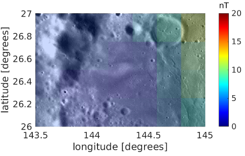
Figure 1: Swirl in Mare Moscoviense: magnetic flux density [10] overlaid on Lunar Reconnaissance Orbiter (LRO) Wide Angle Camera (WAC) mosaic [11]. The maximum magnetic flux density of this region is 11.4nT.
Data and Methods:
This study utilizes normalized spectra of the M3 instrument [12] and our recent space weathering simulation framework [9]. Additionally, we analyze the magnetic flux density maps of [10]. The M3 data are processed with the method described in [13,14,15] by applying topographic, thermal [16] and roughness correction [15, 17]. State-of-the-art space-weathering models such as [9, 18, 19, 20, 21] build upon the current distinction into nanophase iron particles (npFe) that are responsible for reddening and darkening and larger microphase iron particles (mpFe) that only cause darkening [18, 22]. We devised an ab-initio Mie-modeling approach [9] that is used to determine the amount of npFe and mpFe associated with the Mare Moscoviense swirl and the reference region around the craters Bessel F and G. We sample pairs that consist of a spectrum of typical immature soil (either on-swirl or fresh mare crater) and one from a nearby mature mare location, so that it can be safely assumed that the soil composition is identical. Finally, a non-linear optimization scheme used to estimate the amount of npFe and mpFe that is necessary for the modeled immature spectra to best match their corresponding observed mature spectra [9].
Results:
The swirl structure near Mare Moscoviense on the lunar farside is unique in the sense that the magnetic flux density given by [10] at the surface is mostly below 10nT (see Figure 1), while other swirls are associated with magnetic anomalies of several hundred nT [2, 10]. In Figure 2 the best-fit abundance of npFe and mpFe for the swirl are shown at their corresponding on-swirl locations. In Figure 3 the best-fit abundances are shown for the fresh mare craters. The resulting deviations between the measured and modeled mature spectra are very low (for a detailed discussion see [9]). Both regions show a strong correlation between mpFe and npFe weight percentages (Mare Moscoviense: r = 0.978; Bessel F/G: r = 0.962). This trend is illustrated in Figure 4. Consequently, a higher abundance of npFe corresponds to more mpFe in both regions. This trend appears to be largely linear for both regions, but with slightly different slopes.
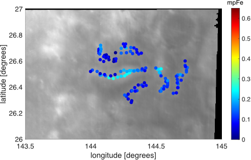
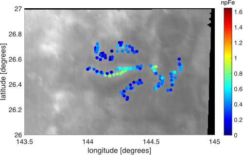
Figure 2: Best-fit mpFe and npFe weight percentages at the Mare Moscoviense swirl overlaid on the 1.579 μm reflectance derived from the M3 data set [12, 23].
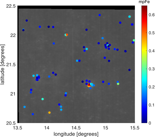
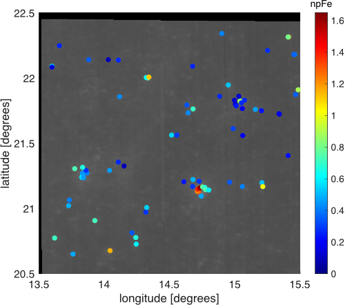
Figure 3: Best-fit mpFe and npFe weight percentages in the Bessel F and G region overlaid on the 1.579 μm reflectance derived from the M3 data set [12, 23].

Figure 4: Weight percentage differences of mpFe and npFe particles between fresh and mature spectra (crater data from [9]).
Conclusion:
The spectral differences at the Mare Moscoviense swirl correspond to a difference in maturity even without a relevant magnetic field that would shield the surface from space weathering. This means that magnetic shielding alone cannot explain the origin of this swirl. A possible explanation for the immaturity is the resurfacing of immature regolith by cometary gas as suggested by [5] and described for a landing rocket jet by [6]. The linear correlation between the npFe and mpFe values is another clue that both types of particles are created by similar processes.
[1] L.L. Hood and G. Schubert, 1980. Science, 208(4439):49–51.
[2] B.W. Denevi et al., 2016. Icarus, 273:53–67.
[3] R.A. Bamford et al., 2016. Astrophys. J., 830(2).
[4] P.H. Schultz and L. J. Srnka, 1980. Nature, 284:22–26.
[5] V.V. Shevchenko, 1993. Astronomy Reports, 37: 314–319.
[6] Y. Wu and B. Hapke, 2018. EPSL, 484:145–153.
[7] M. Hess et al., 2020. Astronomy and Astrophysics, in press.
[8] D.T. Blewett et al., 2011. JGR Planets, 116(E2).
[9] K.S. Wohlfarth et al., 2019. The Astronomical Journal, 158(2):80.
[10] H. Tsunakawa et al., 2015. JGR Planets, 120(6):1160–1185.
[11] R.V. Wagner, et al., 2015. LPSC XXXXVI, abstract #1473.
[12] C.M. Pieters et al., 2009. Curr. Sci., 96: 500–505.
[13] C. Wöhler et al., 2017. Science Advances, 3: e1701286.
[14] C. Wöhler et al., 2017. Icarus, 285:118 – 136.
[15] A. Grumpe et al., 2019. Icarus, 321:486 – 507.
[16] Y. Shkuratov et al., 2011. PSS, 59(13):1326 – 1371.
[17] B.J.R. Davidsson et al., 2015. Icarus, 252:1–21.
[18] P.G. Lucey and M. A. Riner, 2011. Icarus, 212(2): 451 – 462.
[19] D. Trang and P. G. Lucey, 2019. Icarus, 321:307– 323.
[20] S. Gou et al., 2020. EPSL, 535:116117.
[21] A. Penttilä et al., 2020. Icarus, 345:113727.
[22] C.M. Pieters and S.K. Noble, 2016. JGR Planets, 121(10):1865–1884.
[23] NASA and JPL. Planetary data system. https://pds-imaging.jpl.nasa.gov/volumes/m3.html, 2019.
How to cite: Hess, M., Wohlfarth, K., Wöhler, C., Berezhnoy, A. A., Bhatt, M., and Bhardwaj, A.: Space Weathering Trends at the Mare Moscoviense Swirl, Europlanet Science Congress 2020, online, 21 Sep–9 Oct 2020, EPSC2020-716, https://doi.org/10.5194/epsc2020-716, 2020.
Introduction
Small solar system objects may occasionally become captured temporarily by planets. Theoretical models (Granvik et al. 2012, Fedorets et al. 2017) predict the existence of a steady-state population of these objects, also known as minimoons, also in the Earth-Moon system. Only one minimoon, 2006 RH120 has been discovered until recently (Kwiatkowski et al. 2009). Since minimoons spend a significant amount of time in Earth’s vicinity, they have been identified as outstanding targets for in situ exploration, or test cases for initial steps of asteroid resource utilisation (Granvik et al. 2013, Chyba et al. 2014, Brelsford et al. 2016, Jedicke et al. 2018). Moreover, not only are minimoons outstanding targets to constrain the size-frequency distribution of metre-sized asteroids (Harris & D’Abramo 2015, Granvik et al. 2016, Tricarico 2017, Brown et al. 2002), but also for studying the structure of the smallest asteroids. However, until now, the observational evidence of the minimoon population has been lacking.
Observations
The object 2020 CD3 was discovered on February 15th 2020 at the Mt. Lemmon station of the Catalina Sky Survey, and was noticed to be on a geocentric orbit the following night. We report the results of the astrometric and photometric observational campaign to characterise 2020 CD3 performed by Gemini North, LDT, NOT, CFHT, CSS, and other telescopes during spring 2020. By investigating the solar radiation pressure signature on the astrometry of 2020 CD3, and broad-band photometry, we present evidence that 2020 CD3 is indeed the second temporary natural satellite in the Earth-Moon system. We describe its discovery circumstances, physical characterisation, rotational period and orbital evolution.
Discussion
Using 2020 CD3 as an example case, we discuss the challenges of discovering minimoons with contemporary surveys. For the first time, we are able to compare the observational evidence of minimoons with the theoretical models. We also assess the capture duration and rotation period of 2020 CD3 in context of simulation and similar objects. Finally, we compare the origin of minimoons as captured objects from the NEO population against their origin as lunar ejecta, and show why the first mechanism is dominant.
Prospects
The discovery of 2020 CD3, and the comparison to discovery predictions with other surveys (Bolin et al. 2014), assures that the expectation of discovery of tens of minimoons with LSST is realistic (Fedorets et al. 2020). With the anticipated growth of the population of minimoons, the path for further exploration of minimoons is foreseen.
References
Bolin et al. (2014), Icarus 241, 280
Brelsford et al. (2016), PSS, 123, 4.
Brown et al. (2002), Nature, 420, 294.
Chyba et al. (2014) JIMO, 10(2), 477.
Fedorets et al. (2017) Icarus, 285, 83.
Fedorets et al. (2020), Icarus, 338, 113517.
Granvik et al. (2012), Icarus, 218, 262.
Granvik et al. (2013) in V. Badescu ed. Asteroids: Prospective Energy and Material Resources, 151.
Granvik et al. (2016), Nature, 530, 303.
Harris & D’Abramo (2015), Icarus, 257, 302.
Jedicke et al. (2018) FrASS, 5, A13.
Kwiatkowski et al. (2009), A&A, 495, 967.
Tricarico et al. (2017), Icarus, 284, 416.
How to cite: Fedorets, G., Micheli, M., Jedicke, R., Naidu, S. P., Farnocchia, D., Granvik, M., Moskovitz, N., Schwamb, M. E., Weryk, R., Wierzchos, K., Christensen, E., Pruyne, T., Bottke, W. F., Ye, Q., Wainscoat, R., Devogele, M., and Buchanan, L. E. and the et al.: Characterisation of 2020 CD3, Earth’s second minimoon, Europlanet Science Congress 2020, online, 21 Sep–9 Oct 2020, EPSC2020-658, https://doi.org/10.5194/epsc2020-658, 2020.
Asteroids have remained mostly the same for the past 4.5 billion years, and provide us information on the origin, evolution and current state of the Solar System. For the physical characterization of asteroids, one of the best data sources is photometry: the measurement of the disk-integrated brightness of the asteroid. An asteroid's lightcurve (i.e. the dependency of the brightness as a function of time) is indicative of its surface scattering properties, as well as its shape and the state of spin.
In this work, we apply novel Bayesian inverse methods (Muinonen et al., A&A 2020, in revision) to derive phase curve parameters from photometric lightcurve observations. Our aim is to validate and expand the existing analyses by applying the methods to of the order of tens to hundreds of asteroids using photometric data from the Gaia Data Release 2 (Gaia Collaboration, Spoto et al., A&A 616, A13, 2018) and ground-based photometry (Durech et al., A&A 513, A46, 2010) from Database of Asteroid Models from Inversion Techniques (DAMIT). We derive phase curve linear slopes by using four techniques: 1) convex inversion on all data, 2) convex inversion on all data with fixed rotation parameters from DAMIT, 3) ellipsoid inversion on Gaia DR2 data only, and 4) ellipsoid inversion on Gaia DR2 data only with fixed rotation parameters from DAMIT. Finally, we compare the obtained slope parameters with the presumed Bus-DeMeo (DeMeo et al., Icarus 202, 160, 2009) taxonomic classes of the asteroids, and study possible correlations with the geometric albedos. The Gaia photometry has milli-magnitude precision and is thus extremely valuable when used to carry out asteroid taxonomic classification.
How to cite: Martikainen, J., Fedorets, G., Penttilä, A., and Muinonen, K.: Asteroid phase curve parameters from Gaia photometry, Europlanet Science Congress 2020, online, 21 Sep–9 Oct 2020, EPSC2020-654, https://doi.org/10.5194/epsc2020-654, 2020.
Asteroids are classified into different taxonomic groups according to their spectral reflectance properties in the visual and near-infrared (Vis-NIR) wavelengths. The spectral properties of the asteroid surfaces can be related to the material of the surface. There are a few taxonomic systems for asteroids, the most recent being the so-called Bus-DeMeo taxonomy (B-DM, DeMeo et al., Icarus 202, 2009). Usually, the exact wavelengths used in the taxonomic system are tied up with the particular survey data that was used to create the taxonomy. With the B-DM taxonomy, it is the SMASSII survey extended to near-infrared with the NASA IRTF telescope observations, and the wavelengths are 0.45–2.45 µm.
The ESA space observatory Gaia will produce a significant number of low-resolution asteroid spectra over the 0.33–1.05 µm wavelength range in the Data Release 3 and the final data releases. There is an evident need for evaluating the surface properties of these asteroids using the Gaia data. For example, the list of taxonomic classifications for asteroids, maintained in the NASA Planetary Data System, has 2,600 asteroids with some taxonomic class (Neese, C., Ed., NASA Planetary Data System, 2010), but the Gaia data will eventually contain about 100,000 asteroid spectra.
There is a plan to provide a new asteroid taxonomy using the Gaia observations (Delbo et al., PSS 73, 2012). However, a link to existing taxonomic systems such as B-DM would be highly valuable. In this work, we study the possibility to use feed-forward artificial neural network for asteroid spectral classification. We show that the classification accuracy can remain on a reasonably good level even if the B-DM classification is done with the neural network that is trained to use only data having wavelengths in the 0.45–1.05 µm range, which is the overlapping region with the Gaia and the original B-DM systems. This tool can provide the B-DM taxonomic classification for all the asteroids with Gaia spectroscopy.
Acknowledgements: Research supported, in part, by the Academy of Finland (project 325805).
How to cite: Penttilä, A., Hietala, H., and Muinonen, K.: Asteroid taxonomy using artificial neural networks, Europlanet Science Congress 2020, online, 21 Sep–9 Oct 2020, EPSC2020-3, https://doi.org/10.5194/epsc2020-3, 2020.
Stellar occultations provide an instantaneous relative astrometric measurement, as the position of the asteroid center of mass, at the mid-time of the event, is very close to the that of the occulted star. If this target star has an independently measured, accurate position, then the asteroid astrometry can be determined at a similar level of uncertainty. This fact is being routinely exploited, for instance, to improve the orbit of distant Trans-Neptunian Objects after a positive detection of an occultation, thus enhancing the probability of observing subsequent events. However, the same approach can be applied more extensively to the whole available data set of stellar occultations, mainly involving Main Belt asteroids (~5 000 events, for ~1 200 asteroids). We present the results obtained so far in this domain.
The exploitation of stellar astrometry from the Data Release 1 of Gaia has already shown the strong potential for such an approach. However, recent advances have made possible to reach a new level of accuracy.
The first innovation involves a more refined data reduction for occultation astrometry, taking into account differential relativistic effects. The new procedure also provides a more realistic error model, that takes into account both the reported measurement uncertainty, derived from each light curve of an event, and the errors on the position of the occultation chord relative to the asteroid center of mass.
The second major progress is the publication of the new data release by Gaia (DR2) in April 2018, providing nearly the full astrometric performance of the mission, providing proper motions and parallaxes for a large fraction of the stars.
Nevertheless, the exploitation of these data requires some additional care to be effective.
First of all, to exploit asteroid astrometry referred to Gaia DR2, a de-biasing (correction of local systematic errors) must be run on ground based astrometry, when this was reduced by pre-DR2 catalogues. We have recently completed the de-biasing procedure for all 14 099 asteroids present in DR2, and for all the asteroids that produced occultations in the past.
The second critical aspect are the subtle corrections to be applied to the DR2 catalogue to mitigate the impact of a reference frame rotation found in the catalogue (Lindegren 2020).
With this approach, we attempted to improve the asteroid orbits with all archival astrometry included, and with occultations only, for what can be considered to be the best possible exploitation of occultation astrometry to date. We illustrate the obtained performance, and the limitations of the methods for observed events with a small number of observed chords.
With the expected improvement in asteroid orbits brought by Gaia DR2 (and DR3 to come) a large number of smaller asteroids will provide reliable predictions and contribute more systematically to accurate astrometry, to the advantage of the detection of subtle dynamical effects (such as Yarkovsky) directly in the Main Belt.
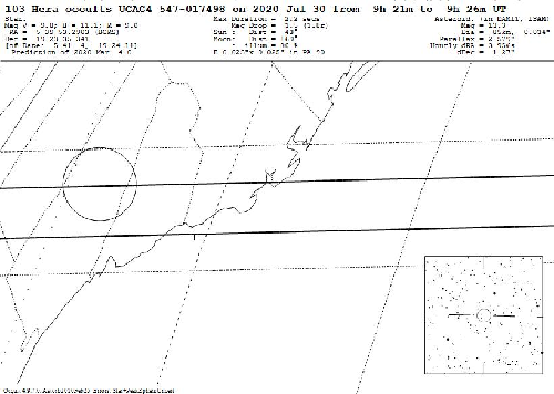
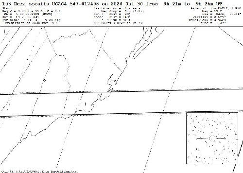
Fig 1. Prediction by Steve Preston (IOTA) to occultation of (103) Hera on 2020-07-30, using MPC data, compared to our prediction, combining MPC and Gaia. The resulting path uncertainty decreases by a factor of 6 with our method, a decrease verified for most of the asteroids present in GDR2, as the average decrease in the full sample was by a factor of ~5.
How to cite: Ferreira, J., Spoto, F., Tanga, P., and Machado, P.: Performance of occultation astrometry with Gaia DR2, Europlanet Science Congress 2020, online, 21 Sep–9 Oct 2020, EPSC2020-594, https://doi.org/10.5194/epsc2020-594, 2020.
Binary Transneptunian Objects (TNOs) have remained virtually unaltered since the formation of the solar system. They can therefore provide valuable insights into the history and properties of objects from the outer solar system, such as object compositions and dynamical history, including the effects of planetary migration on primordial planetesimal populations. Benecchi et al. 2009 measured the colours of 23 TNO binaries using the Hubble Space Telescope (HST), reporting a strong correlation between primary-secondary F606W-F814W colours. Marsset et al. 2020 extended this work into the NIR, adding a further three TNO binary objects with accurate colour measurements made using the Gemini-North telescope which indicated a similar colour correlation in the infrared.
We aim to increase the number of binary TNOs with accurate NIR colour measurements by reprocessing data available in the HST archive using a consistent MCMC-based point spread function (PSF)-fitting algorithm. We explore both the position and brightness parameter space for the binary components. Tiny Tim (Krist et al., 2011) PSFs are generated for each component and planted in a model image that is compared with the HST archive image to identify best-fit PSF parameter values. These values are then used to produce and subtract a final model image, providing accurate likelihood estimates for the in-image position and photometric brightness of each component.
We will present the results of applying the algorithm to archival data of 24 known binaries, including both optical and NIR colour measurements of both binary components. We will also provide a measure of our sensitivity to binary component separations and brightness ratios. Our results will be compared to the correlated colours observed by Benecchi et al. (2009) and Marsset et al. (2020).
References:
S. D. Benecchi, K. S. Noll, W. M. Grundy, M. W. Buie, D. C. Stephens, andH. F. Levison. The correlated colors of transneptunian binaries. Icarus, 200(1):292–303, Mar 2009. doi: 10.1016/j.icarus.2008.10.025.
J Krist, R Hook, and F Stoehr. 20 years of hubble space telescope opticalmodeling using tiny tim, 2011. URLhttps://doi.org/10.1117/12.892762.
Micha ̈el Marsset, Wesley C. Fraser, Michele T. Bannister, Megan E. Schwamb, Rosemary E. Pike, Susan Benecchi, J. J. Kavelaars, Mike Alexandersen, Ying-Tung Chen, Brett J. Gladman, Stephen D. J. Gwyn, Jean-Marc Petit, and Kathryn Volk. Col-OSSOS: Compositional Homogeneity of Three KuiperBelt Binaries.The Planetary Science Journal, 1(1):16, June 2020. doi:10.3847/PSJ/ab8cc0.
How to cite: Smith, R., Fraser, W., and Fitzsimmons, A.: Characterisation of Transneptunian Binaries in the HST Archive., Europlanet Science Congress 2020, online, 21 Sep–9 Oct 2020, EPSC2020-263, https://doi.org/10.5194/epsc2020-263, 2020.
Characterisation of the V-type asteroid population may help to comprehend the planetesimal formation and evolution. Asteroid phase-curves are known to relate to surface properties such as asteroid taxonomy, surface roughness, particle size distribution, albedo and many others, providing insight into surface properties of the V-types.
Gil-Hutton et al. (2017) showed that the basaltic asteroids display two distinct polarimetric behaviors, which they attributed to the regolith particle size. Considering that phase-curve parameters relate to surface and regolith properties, they may verify those distinct behaviors.
We observed about 20 asteroids during around 250 nights (over 500 fragmental lightcurves) to obtain high quality phase curves. We fitted the standard H,G; H,G1,G2, and H, G12 phase functions, limiting them to physical solutions only. This greatly extends the sample of well determined phase-curves for the underrepresented V-types. For asteroids with data from multiple oppositions we used a simultaneous fit assuming the same slope parameters in all apparitions and different absolute magnitude values. From these data we also derived the G12* parameter to be used in single parameter phase functions recommended for fitting low quality photometry. We do not find substantial evidence for any clustering into distinct phase curve parameters groups as suggested by Gil-Hutton et al. 2017. Only one asteroid (2763 Jeans) shows an exceptionally high G2 value.
Further work should be conducted to determine slope parameters of more V-types to further verify the division of V-type asteroids into two distinct groups. Obtaining phase curves of non-Vestoids (such as those in the mid and outer Main Belt) may also help clarify if the division into distinct V-type groups is due to particle size or mineralogical differences.
How to cite: Oszkiewicz, D. and the SONATA13: Characterisation of V-type asteroids using phase-curves, Europlanet Science Congress 2020, online, 21 Sep–9 Oct 2020, EPSC2020-699, https://doi.org/10.5194/epsc2020-699, 2020.
Abstract
We have developed the first database of asteroid regolith properties: fifty asteroids so far, to aid space resource utilisation workers. The physical parameters: grain density, grain size, near surface bulk density and porosity are provided of a collection of the asteroids. The strength of our method is that it combines three types of information: 1) spacecraft-based, in-situ data, 2) laboratory-based meteorite samples, and 3) telescopic, remote data, such as from polarisation-- the joint usage which amplifies the success and the probability of gaining new information. The database is also uniquely robust, due to its large number of crosschecks for the database's regolith parameters. Theoretical studies provide additional crosschecks. See Figure 1. A critical perspective is the assignment of the spatial scales where the bulk density and porosity of an asteroid is related to the average density and porosity of its constituent rocks, which is further distinguished from the average density of the mineral assemblages within the rocks.
Introduction
In-space resource utilisation will provide an extension of our SpaceShip Earth to include space infrastructures for, and of, our robots that are orbiting the Earth and traveling beyond. With such space resources, we can service, recycle, or build anew, without the limitations of carrying the resources from the Earth. Telecommuncations, Earth observations, planetary research, extraterrestrial life explorations, are just a few examples, which can be implemented cheaper and more efficiently using resources in space.
Despite the asteroid mining industry’s shift to smaller companies since 2018, it is no longer a question of ‘if’ but of ‘when’. The endeavour of the in-space utilisation of asteroid resources have several attractive features over their lunar and Martian counterparts, in that their low gravity, large quantities,and tiny sizes lead to different legal regimes for their utilisation and hence are more attractive for private funders to build in space with these resources.
The derived products for the asteroid regolith properties are currently following this flowchart:

Figure 1: Flowchart of the methodology of the Asteroid Regolith Database.
Meteorite Samples as Proxies?
One particular goal and feature of the Asteroid Regolith Database (ARD)'s robust strengths, is the use of proxies in lieu of asteroid samples to determine an asteroid regolith's porosity. This year, we sought to answer the following question before we can trust that meteorites can indeed be porosity proxies: Are meteorites already compressed in porosity before they enter the Earth’s atmosphere?
Empirical Support:
How to use such a Meteorite Proxy in the ARD:
- IF data for an asteroid is missing or sparse, but is linked to a meteorite analog, then one can compare the measured meteorite porosity of the analog material with the inferred bulk density of the material, to deduce density of the regolith grain.
- Thermal conductivity meteorite lab data additionally provides information to derive asteroid regolith particle sizes and particle porosity and crosschecks.
- However, IF the assumption is not valid, then one can still fit a functional form rearranging the thermal inertia equation, ρ = Γ2/(kcp) and keeping track of scales (ρrock, ρgrain, φrock, etc., for example: ρrock = (1−φrock)ρgrain and proceed.
- IF one assumes that it’s valid to match meteoritic thermal inertia versus porosity data to its asteroidal counterpart, then one can relate regolith parameters, to derive a functional form that relates thermal inertia and porosity. Such an assumption will allow one to fill in possible gaps in data, to help mitigate any lack of thermal inertia data to derive porosities for the asteroid regolith database.
-
In either case, we will have a function form that provides a Γ versus porosity relationship when we do not have thermal inertia data. The estimates of the accuracy will need to include the laboratory data acquisition errors along with the model fitting errors.
Summary and Conclusions
We have 50 asteroids thus far in our Asteroid Regolith Database. See the TREX website for the list: https://trex.psi.edu/
Upon investigating the meteorite proxy question, our Conclusions point to a clear need for more meteorite samples, measured in SEM in consistent ways.
Acknowledgements
The ARD has been supported, in part, by several funding organisations: (Vaivode): the University of Latvia Institute of Astronomy small research projects funding, and (Graps): the NASA Toolbox for Research and Exploration (TREX) project, which is a node of NASA’s Solar System Exploration Research Virtual Institute 2016 (SSERVI16) Cooperative Agreement (NNH16ZDA001N).
How to cite: Graps, A. L., Vaivode, M., Consolmagno SJ, G. J., and Britt, D. T.: An Asteroid Regolith Database for ISRU, Europlanet Science Congress 2020, online, 21 Sep–9 Oct 2020, EPSC2020-939, https://doi.org/10.5194/epsc2020-939, 2020.
Estimation of asteroid sizes from the observed thermal emission are performed by comparing the flux modeled from simple thermal models and thermophysical models (TPMs). The accuracy of the diameter estimate is dependent on the accuracy of the modeled surface temperatures, which are calculated differently among these models. Simple thermal models, like the often-chosen NEATM, do not account for subsurface heat conduction whereas thermophysical models explicitly account for it. This neglect of heat transport can, generally speaking, result in the overestimation of diameters when simple thermal models are used (Spencer, et al. 1989) because nighttime thermal emission is neglected by simpe thermal models (the NESTM model being the exception). Mommert et al. (2019) showed that NEATM diameter fits to NEAs are reasonably accurate (i.e. little systematic bias) when the solar phase angle of observation is <65°, however became increasingly inaccurate for phase angles >65°. On the other hand, TPMs are thought to provide highly accurate diameters regardless of the observing circumstances or physical properties of the surface because they include heat conduction.
Nearly all TPMs compute surface temperatures over a diurnal timescale, over which the solar energy input is held constant. However, as the case with high-eccentricity NEAs, a potentially overlooked effect on diameter determination is the influence of rapidly-change in solar heating. Because these objects experience large, rapid changes in the amount of absorbed sunlight, heat conducted into the subsurface at small heliocentric distances will affect surface tempertures at larger heliocentric distances. Figure 1 below demonstrates that this effect is more pronounced for larger orbital eccentricities.

Figure 1. Discrepancy (orbTPM-diTPM) in the maximum daily temperature at different heliocentric distances for a hypothetical asteroid with varying orbital eccentricity. Dots indicate time steps separated by ~2 days. Open circles show the median values of temperature discrepancy and heliocentric distance. A positive value for the discrepancy indicates a larger orbTPM temperature.
In this work we compare two TPMs: one with a fixed solar energy input over a diurnal timescale, diTPM, and another that models surface temperatures over an entire orbit, orbTPM. We compare the disk-integrated fluxes of each model in order to investigate and characterise any discrepancy. Emitted thermal flux is directly proportional to size, thus the flux discrepancy between the two models is used to quantify any bias in diameter determination when the diTPM is used.
The potential effects of thermal inertia, rotation period, spin axis, and phase angle on this discrepancy are considered. Finally, we employ the orbTPM on a few asteroids observed in the thermal infrared and postulate on the implications on thermal modelling of NEAs as a population.
How to cite: MacLennan, E. and Granvik, M.: Biases in TPM-derived Diameters for High-Eccentricity NEAs, Europlanet Science Congress 2020, online, 21 Sep–9 Oct 2020, EPSC2020-989, https://doi.org/10.5194/epsc2020-989, 2020.
Introduction
Optical properties are required information for correct models of the early solar system and protoplanetary disks. To this day the properties used in the models are mostly provided by laboratory studies of primitive analogs. Comets provide us with a closer analog to the protoplanetary material but have been, until recently, difficult to observe. Rosetta has given us the unique opportunity to observe with unprecedented accuracy.
The Microwave Instrument for the Rosetta Orbiter (MIRO) (Gulkis et al. 2007) measured the thermal radiation emitted from the subsurface of comet 67P/Churyumov-Gerasimenko (hereafter 67P). MIRO operated at millimetre (hereafter MM) and sub-millimetre (hereafter SMM) wavelengths with corresponding frequencies of 188.2 GHz (1.594 mm) and 562.8 GHz (0.533 mm), respectively.
The thermal radiation received by MIRO is strongly dependant on the sub-surface material properties, mainly its temperature and optical constants. Our aim is to derive from these observations the complex refractive index of the material of comet 67P's subsurface. To achieve this, we match the brightness temperatures measured by MIRO with synthetic values derived from a one-dimensional thermal model of the subsurface combined with radiative transfer models.
MIRO data selection
MIRO data used in this study are taken from the ESA Planetary Science Archive. We selected only those measurements where the orbiter was close to the surface of the nucleus, to minimise the MIRO beam size on the nucleus and, thus, to be able to focus on specific areas of the comet. Additionally, we set our focus on flat areas, which allows us to use a one-dimensional thermal model.
Just before equinox in March 2016, the Rosetta orbiter was 11 km from the surface of 67P, observing the relatively flat region Imhotep (Auger et al. 2015). This region is located on the bottom of the big lobe and consists of four sub-regions, a,b,c and d (Thomas et al. 2018). We analysed MIRO measurements in sub-region 'a', as it is the smoothest and closest to the equator (Thomas et al. 2018). Fig. 1 illustrates the location of sub-region 'a' on the nucleus.
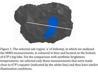
Fig. 2 shows the brightness temperatures MIRO measured in Imhotep's sub-region 'a' in March 2016 plotted against the effective local solar hour on the nucleus of comet 67P. Here, only measurements that are made at distances smaller than 20 km and with low emission angles were selected.
For the comparison with synthetic brightness temperatures, we filtered those measurements in sub-region 'a' that were made close to 67P's equator (see white line in Fig. 1) and, thus, experience similar illumination conditions. The three suitable temperature sets we found, two at night and one at day, are highlighted in Fig. 2 with darker colours.

Thermophysical simulation
The one-dimensional thermal model described in Gundlach et al. 2020 is based on a homogeneous medium and solves the heat transfer equation using the Crank-Nicolson method. We simulated 1000 cometary days, using as input parameters 67P's precise heliocentric distance and the illumination angle of the analysed area on the surface. The last simulated day refers to the day of the selected MIRO measurement. The output of the thermal model is a temperature profile with depth, which serves as input for the raytracing and radiative transfer models.
We modelled both, a homogeneous and a inhomogeneous medium (the inhomogeneous medium was built using pebble radii ranging from 3 mm to 6 mm). While for the former only heat conduction is relevant, the latter requires heat transfer by conduction and radiation.
Raytracing
The thermal emission of the comet measured by MIRO is modelled by raytracing, applying geometric optics through a three-dimensional structure of spherical pebbles, packed randomly at a volume filling factor of ∼0.58, close to a value of 0.55 expected for random loose packing (Onoda and Liniger 1990). Rays are traced backwards, from MIRO down to the comet, where they are reflected or absorbed. The complex refractive index of the pebble material is varied in a range n = 1.0 ... 1.4 for the real part and k = 0.001 ... 0.02 for the imaginary part. For the larger wavelength, the decrease rate of the number of rays with depth in the comet has been compared to attenuation coefficients calculated by waveoptics (FDTD, for pebble radii 3mm to 6mm, n = 1.2, k = 0.001, 0.003) and have been found to be similar. For the smaller wavelength, geometric optics then should be valid as well. The raytracing returns a depth profile e(x) of the starting points of rays contributing to the thermal emission and the directional-hemispherical reflectivity Rdh from which, after Kirchhoff's law (Hapke 1993), the emissivity of the cometary surface results.
Synthetic temperatures
The raytracing's emission profile e(x) is convolved with the intensity profile Bν(T(x)), where Bν is Planck's function, to get the temperature dependent emission profile. Integration over depth considering reflectivity Rdh yields the total comet's intensity. The additional reflected 3K cosmic background radiation can be neglected. Thus, the synthetic temperature Tν is given by:
Tv = Bv-1 ( (1 - Rdh) ∫ BvT(x)e(x) dx )
Conclusion
By using a one-dimensional thermal model combined with both a raytracing and radiative-transfer model, we were able to derive constraints on the subsurface material properties, namely its optical properties (real and imaginary part of the index of refraction) down to around 10 cm beneath the surface. We will present the models in detail as well as the optical properties we derived from this study. Reliable optical data are important as they provide the community with values of optical constants representative of the early solar system, protoplanetary disks and debris disks.
Acknowledgements
This study was performed as part of the DFG Research Unit ''Debris Disks in Planetary Systems".
References
Auger A., et al., 2015, A&A, 583, A35
Gulkis S., et al., 2007, Space Sci. Rev., 128, 561
Gundlach B., et al., 2020, MNRAS, 493, 3690
Hapke, B., 1993, Cambridge University Press, Chapter 13.D
Onoda, G., Liniger, E., 1990, Phys. Rev. Lett., 64, 2727
Thomas N., et al., 2018, Planet. Space Sci., 164, 19
How to cite: Bürger, J., Gundlach, B., Lethuillier, A., Glißmann, T., Blum, J., Mutschke, H., and Höfer, S.: Sub-millimetre/millimetre extinction of real protoplanetary matter derived from Rosetta/MIRO observations on comet 67P, Europlanet Science Congress 2020, online, 21 Sep–9 Oct 2020, EPSC2020-140, https://doi.org/10.5194/epsc2020-140, 2020.
We present a summary of the radar experiments performed with the Arecibo Observatory Planetary Radar system during 2019-2020. Located in Puerto Rico (18° 20' 36.6" N, 66° 45' 11.1" W) the Arecibo Observatory S-band (2380 MHz) radar system is capable of transmitting up to 1MW of power and uses the William E Gordon Telescope antenna of 305 m. The planetary radar science group focuses on performing follow-up (post discovery) observations of known small bodies as well as recently discovered ones. Priority is given to objects on the CNEOS Sentry impact risk list, those classified as Potentially Hazardous (PHA’s) and those that are potential spacecraft mission targets (NHATS). Although currently operating at 35% power capacity, Arecibo has observed 92 objects since September 2019 to abstract submission date, distributed as: 61 recently discovered objects, 28 PHA’s, 2 planets and 1 comet. We present here some science highlights of this year's observations of near-Earth objects (NEOs), including radar delay-Doppler images of 2020BX12, 2011WN15, 481394 (2006 SF6) and 162082 (1998HL1).
Introduction
The Arecibo Observatory is the largest and most powerful planetary radar system in the world, successfully observing up to 130 asteroids a year. Funded by the NASA-NEO Observations program, the ground-based observations done using the S-band (2380 MHz, 12.6 cm) radar systems are a highly cost effective and rapid tool to constrain physical and dynamical properties of the targets in comparison to space missions. This Instrument has the capability of transmitting a signal with or without phase modulation, providing extremely accurate astrometry measurements (range and radial velocity) on newly discovered objects, and track changes in the orbit of previously observed ones, such as those due to non-gravitational perturbations. Besides orbital characterization, radar data provides constraints on the object's size and rotation rate, is responsible for the discovery of satellites [1,2] and for some cases can identify the shape and near-surface (meter-scale) structures up to a few wavelengths deep.
Methods
The S-band system transmits a circularly polarized wave, and receives both the same-sense circular (SC) and opposite-sense circular polarization (OC) as transmitted. Radar observations usually start by a continuous-wave measurement to obtain the Doppler frequency spectrum of the echo. The measured Doppler spectrum bandwidth provides initial limits for rotation period and the object’s apparent diameter. From the measured received backscattered power in these two orthogonal states of polarization, it's possible to calculate the target's circular polarization ratio. Defined as the ratio of the SC and OC echo and commonly used as an indicator of the surface reflection properties. For targets with a relatively high signal-to-noise-ratio (SNR) we use phase modulation to produce delay-Doppler images, with range resolution as fine as 7.5 m per pixel in some cases. These images aid in the estimation of objects' diameter and provide an idea of the body's shape.
Results
Some highlights of our observations include: 162082 (1998 HL1) observed on October 25-28, 2019 with a delay-Doppler resolution of 75 m/px, its apparent diameter is estimated at 270 m, and its rotation period at approximately 11 hrs. Contact binary 481394 (2006SF6) was observed on November 11-15, 2019, with a delay-Doppler resolution of 7.5 m/px showing a maximum visible extent of 240 m. The rotation period is estimated to be 11.3 hrs and it was observed at various orientations. 2011 WN15 was observed on December 12-13, 2019, with a delay-Doppler resolution of 7.5 m/px providing an estimate on diameter of 900 m, and a rotation period of up to 4 hours. 2020 BX12 observation on February 4-5, 2020, led to the discovery of a secondary body, images with delay-Doppler resolution of 7.5 m/px, showed a diameter of 165 m for the primary and no more than 70 m for the secondary. The apparent rotation period for the primary is about 2.8 hrs and 49 hrs or less for the secondary.
Acknowledgements:
The Arecibo Planetary Radar Program is fully supported by NASA’s Near-Earth Object Observations Program in NASA’s Planetary Defense Coordination Office through grant no. 80NSSC19K0523 awarded to University of Central Florida (UCF). UCF manages the National Science Foundation facility under a cooperative agreement with Yang Enterprises, Inc. and Universidad Ana G. Méndez.
References
[1] Benner, L.A., Nolan, M.C., Margot, J., Brozovic, M., Ostro, S.J., Shepard, M.K., Magri, C., Giorgini, J.D. and Busch, M.W., 2008, September. Arecibo and Goldstone radar imaging of contact binary near-Earth asteroids. In DPS (pp. 25-03).
[2] Rivera-Valentin, E.G., Taylor, P.A., Virkki, A. and Aponte-Hernandez, B., 2017. (163693) Atira. CBET, 4347, p.1.
How to cite: Zambrano-Marin, L., Virkki, A., Marshall, S., Venditti, F., Hickson, D., McGilvray, A., Devogele, M., Taylor, P., and Rivera-Valentín, E.: Arecibo Science Highlights of Observatory Planetary Radar Observations: 2019-2020, Europlanet Science Congress 2020, online, 21 Sep–9 Oct 2020, EPSC2020-992, https://doi.org/10.5194/epsc2020-992, 2020.
Radar remote sensing is a powerful tool used to image planets, moons, asteroids, and comets with ground-based and orbital instruments. Variations in the backscatter coefficient, or albedo, are related to changes in the near-surface properties. Analyses of radar albedos have revealed polar ice deposits on Mercury (Slade et al., 1992), identified methane lakes on Titan (Stofan et al., 2007), and provided evidence for the ice crusts of Europa, Ganymede, and Callisto (Ostro et al., 1992). Interpretations of radar albedos of asteroids have been used to infer metallic composition, such as for 16 Psyche (Magri et al., 1999), the possible remnant metallic core that is the target of NASA’s Psyche mission. Analyses that combine measurements of radar albedos of asteroids with dielectric models have been used to determine the near-surface porosity of asteroids (Magri et al., 2001; Hickson et al., 2020).
In these models, the radar albedo is used to determine the Fresnel reflectivity of the near-surface, which can then be used to determine the complex index of refraction of the near-surface material, n=√εµ. The index of refraction is a function of the complex permittivity, ε, and the complex permeability, µ. Most minerals are paramagnetic, with permeabilities approaching that of vacuum. As such, many interpretations of the Fresnel reflectivity of planetary surfaces are predominantly concerned with the permittivity. However, some iron oxide minerals are ferromagnetic, and possess permeabilities that can be significantly greater than that of vacuum. The importance of these minerals in interpreting radar backscatter has been identified for Mars, for which iron oxide minerals such as magnetite, hematite, and goethite have been identified in the regolith (Stillman 2006). Earth-based spectroscopic observations of near-Earth asteroid 101955 Bennu, the target of NASA’s OSIRIS-REx mission, hinted at the presence of magnetite on the surface (Cloutis et al., 2013). Spectral data obtained by the OSIRIS-REx spacecraft have recently corroborated these early Earth-based observations (Hamilton et al., 2019). These data, combined with compositional analyses of analogue CI/CM carbonaceous chondrite meteorites, indicate that the surface of Bennu could be comprised up to 10% by magnetite.
In this study, we model the effect of magnetic iron oxides on the radar albedo of asteroids. Since the iron oxide abundance on asteroids is not well understood, we use Bennu as a test case. Laboratory measurements of the magnetic permeability of magnetite have been carried out by several authors, including Pettinelli et al., 2005, Cereti et al., 2007, and Stillman 2006 with application to orbital sounding radar of Mars. The measured permeability in these studies can be extrapolated to a volume fraction of magnetite of 10%, relevant for Bennu as mentioned above, using effective medium approximations. Figure 1 shows the measurements of magnetic permeability of various magnetite mixtures from Pettinelli et al., 2005 and Cereti et al., 2007 fit with the Bruggeman Symmetric mixing model using a permeability of 5.5 for the magnetite phase.

Figure 1: Magnetite mixture permeability measurements from the literature fitted with the Bruggeman Symmetric effective medium model.
At 10% magnetite, this model predicts an effective permeability of 1.21. This corresponds to an increase of the index of refraction by a factor of √1.21 = 1.1, or 10%. For a smooth surface at normal incidence, the radar albedo, σ, is equal to the Fresnel reflectivity:
σ = abs((√εµ - 1)/(√εµ + 1))^2.
Ignoring the imaginary part (which is often significantly lower than the real part), for a permittivity of 3 and permeability of 1 the above equation gives a radar albedo of σ = 0.072. If we further assume that this surface is comprised of 10% magnetite (and assume that the magnetite’s permittivity has already been incorporated into the effective permittivity of 3), changing the effective permeability to 1.21 increases the radar albedo to σ = 0.097. In this simple example, considering the magnetic effect of 10% magnetite increased the radar albedo by 35% compared with a strictly dielectric model.
We have shown through laboratory measurements from the literature and electromagnetic modeling that iron oxides can increase radar albedos of asteroids appreciably due to their magnetic properties. These magnetic properties must be better understood in the context of asteroids, and their abundances better characterized, for improved interpretation of planetary radar datasets.
References:
Cereti, A., et al. (2007). Electromagnetic measurements on Martian soil analogs: Implications for MARSIS and SHARAD radars in detecting subsoil water. Planetary and Space Science, 55(1-2), 193-202.
Cloutis, E. A., et al. (2013). Possible Causes of Blue Slopes (~ 0.5-2.5 µm) in Carbonaceous Chondrite Spectra. LPI, (1719), 1550.
Hamilton, V. E., et al. (2019). Evidence for widespread hydrated minerals on asteroid (101955) Bennu. Nature Astronomy, 3(4), 332-340.
Hickson, D. C., et al. Modeling the Dielectric Properties of Minerals from Crystals to Bulk Powders for Improved Interpretation of Asteroid Radar Observations. Journal of Geophysical Research: Planets, e2019JE006141.
Magri, C., et al. (1998). Mainbelt asteroids: Results of Arecibo and Goldstone radar observations of 37 objects during 1980-1995.
Magri, C., et al. (2001). Radar constraints on asteroid regolith properties using 433 Eros as ground truth. Meteoritics & Planetary Science, 36(12), 1697-1709.
Ostro, S. J., et al. (1992). Europa, Ganymede, and Callisto: new radar results from Arecibo and Goldstone. Journal of Geophysical Research: Planets, 97(E11), 18227-18244.
Pettinelli, E., et al. (2005). Laboratory investigations into the electromagnetic properties of magnetite/silica mixtures as Martian soil simulants. Journal of Geophysical Research: Planets, 110(E4).
Slade, M. A., et al. (1992). Mercury radar imaging: Evidence for polar ice. Science, 258, 635 – 640.
Stillman, D.E. (2006) Frequency and Temperature Dependence in Electromagnetic Properties of Martian Analog Minerals. Doctoral Thesis, Colorado School of Mines.
Stofan, E. R., et al. (2007). The lakes of Titan. Nature, 445(7123), 61-64.
How to cite: Hickson, D. and Virkki, A.: Modeling the effect of iron oxides on asteroid radar albedos, Europlanet Science Congress 2020, online, 21 Sep–9 Oct 2020, EPSC2020-444, https://doi.org/10.5194/epsc2020-444, 2020.
Please decide on your access
Please use the buttons below to download the presentation materials or to visit the external website where the presentation is linked. Regarding the external link, please note that Copernicus Meetings cannot accept any liability for the content and the website you will visit.
Forward to presentation link
You are going to open an external link to the presentation as indicated by the authors. Copernicus Meetings cannot accept any liability for the content and the website you will visit.
We are sorry, but presentations are only available for users who registered for the conference. Thank you.