Poster presentations and abstracts
Electromagnetic scattering phenomena play a key role in determining the properties of Solar System surfaces based on observations using different techniques and in a variety of wavelengths ranging from the ultraviolet to the radio. This session will promote a general advancement in the exploitation of observational and experimental techniques to characterize radiative transfer in complex particulate media. Abstracts are solicited on progresses in numerical methods to extract relevant information from imagery, photometry, polarimetry and spectroscopy in solid phase, reference laboratory databases, photometric modeling, interpreting features on planetary surfaces, mixing/unmixing methods… Software and web service applications are welcome.
Session assets
At present, the main database of asteroid absolute magnitudes is the Minor Planet Center (MPC). The MPC receives asteroid magnitudes from many observatories in different spectral bands of different photometric systems, but calculates absolute magnitudes for V band of the Johnson photometric system using the HG-function [1]. A comparison of the MPC absolute magnitudes (HMPC) with the dataset of high-quality absolute magnitudes obtained by Pravec et al. [2] revealed systematical differences between these datasets. The new HG1G2 function was recommended by Muinonen et al. [3] to be used for more precise calculating the asteroid absolute magnitudes. This function was calibrated according to good measured magnitude-phase dependences, and the average parameters for major taxonomic classes of asteroids were obtained [4, 5]. Using these average values, it is possible to calculate the absolute magnitudes of asteroids from individual observations at different phase angles. For sparse photometric data, it was suggested to use the two-parameter HG12 system [3, 4, 6].
Recently, large-scale survey programs such as Pan-STARRS and Palomar Transient Factory (PTF) [7, 8] performed new observations, within which absolute magnitudes of asteroids have also been derived. Both datasets are homogeneous, but they were obtained mostly in the Sloan system and then transformed to the Johnson system. Comparison of these datasets of absolute magnitudes with the MPC data showed systematical deviations [7, 8]. It should be noted that the absolute magnitudes of asteroids in the Pan-STARRS and PTF surveys [7, 8] were obtained in the new HG12 system. In addition, the work is continued to obtain the asteroid absolute magnitudes in the new system for PTF and Pan-STARRS datasets [9]. To check the reliability of these datasets and identify systematic deviations, an independent set of high-quality data on absolute magnitudes is required. Thus, we initiated an observational program to determine the absolute magnitudes of several hundred asteroids. Here we present preliminary results of our program.
For our dataset, we used first the data of the asteroid magnitude-phase dependences collected at the Institute of Astronomy of V. N. Karazin Kharkiv National University [5, 10–12]. We also used observational data of asteroids from our other programs and performed new observations of some asteroids [13–14]. We calculated our absolute magnitude dataset in the Johnson V band with a correction for lightcurve variations using the HG1G2 system according to its extension to low-accuracy data [4]. In such manner, we obtained a homogenous dataset of absolute magnitudes of about 300 asteroids in the range from 6.5 to 16 mag. Fig. 1 shows the correlations of the absolute magnitudes from the MPC, Pan-STARRS (HPS), and PTF (HPTF) datasets with those of the Kharkiv dataset (HKH).

Figure 1: Absolute magnitudes of MPC (HMPC), Pan-STARRS (HPS), and PTF (HPTF) vs. those of the Kharkiv dataset (HKH).
We observe a high correlation between our dataset and the other three datasets. There are small differences in the constant terms and slopes that point out some systematical deviations especially for the MPC and the PTF datasets.

Figure 2: Histogram of the absolute magnitude deviations between the Kharkiv and Pan-STARRS datasets.

Figure 3: Histogram of the absolute magnitude deviations between the Kharkiv and MPC datasets.
For the MPC dataset, we found a systematical deviation of about 0.1 mag (Fig. 3). It is less than that obtained in [2] and close to that obtained in [7]. The smallest deviations were found for the Pan-STARRS dataset. This is confirmed by the histogram of absolute magnitude deviations between the Kharkiv and Pan-STARRS datasets presented in Fig. 2. The solid line is a fit to the data using the Gaussian function.
We prepared a preliminary comparative analysis of the asteroid absolute magnitudes between the Kharkiv dataset and the MPC, Pan-STARRS, and PTF datasets. The analysis has shown that the absolute magnitude dataset obtained from the Pan-STARRS survey project is closest to our dataset and can be the most suitable for the determination of diameters or albedos of asteroids.
Acknowledgments
This research has made use of data and/or services provided by the International Astronomical Union's Minor Planet Center.
References
[1] Bowell, E., Hapke, B., Domingue, D., et al. In Asteroids II. Tucson. Univ. Arizona Press. P. 524−556, 1989.
[2] Pravec, P., Harris, A.W., Kušnirák, P., et al. Icarus, 221, 365-387, 2012.
[3] Muinonen, K., Belskaya, I.N., Cellino, A., et al. Icarus, 209, 542–555, 2010.
[4] Penttilä, A. Shevchenko, V.G., Wilkman, O., Muinonen, K. PSS, 123, 117–125, 2016.
[5] Shevchenko, V.G., Belskaya, I.N., Muinonen, K., et al. PSS, 123, 101−116, 2016.
[6] Oszkiewicz, D.A., Muinonen, K., Bowell, E., et al. JQSRT, 112, 1919-1929, 2011.
[7] Veres, P., Jedicke, R., Firzsimmons, A., et al. Icarus, 261, 34-47, 2015.
[8] Waszczak, A., Chang, C.-K., Ofeck, E.O., et al. Astron. J., 150, A75, 2015.
[9] Penttilä, A., Cellino A., Lu X., et al. DPS, 48, No 7, 228, 2016.
[10] Shevchenko, V.G., Belskaya I.N., Lupishko D.F., et al. EAR-A-COMPIL-3-MAGPHASE-V1.0. NASA PDS, 2010.
[11] Shevchenko, V.G., Belskaya, I.N., Slyusarev, I.G., et al. Icarus, 217, 202–208, 2012.
[12] Slyusarev, I.G., Shevchenko, V.G., Belskaya, I.N., et al. LPSC 43, 1885, 2012.
[13] Chiorny, V.G., Shevchenko V.G., Krugly Yu.N., et al. PSS, 55, 986−997, 2007.
[14] Shevchenko, V.G., Mikhalchenko O.I., Belskaya I.N., et al. LPSC 50, Abstract #1771, 2019.
How to cite: Shevchenko, V. G., Mikhalchenko, O. I., Belskaya, I., Chiorny, V., Krugly, Y., Slyusarev, I., Hromakina, T., Dovgopol, A., Gritsevich, M., Muinonen, K., and Penttilä, A.: Comparative analysis of the absolute magnitudes of asteroids with MPC, Pan-STARRS, and PTF datasets, Europlanet Science Congress 2020, online, 21 Sep–9 Oct 2020, EPSC2020-565, https://doi.org/10.5194/epsc2020-565, 2020.
- Abstract
From July 2011 to September 2012, the Dawn spacecraft orbited the large asteroid (4) Vesta. A nearly global coverage of the surface was achieved by the Visible and InfraRed mapping spectrometer (VIR) [1]. The change of CCD temperature during the data acquisition affects the instrument spectral response. As a consequence, the acquired spectra experienced a change in spectral slope. Here we present a method to correct this issue; this method is similar to the one we applied for the VIR VIS data of Ceres [2].
- CCD detector temperature dependencies
The acquisition of VIR data are organized in sequences during which several hyperspectral cubes are acquired. Within a given sequence, which may last several hours, the CCD temperature increases over time, while it goes back down in the time period between two sequences. The increase of CCD temperature induces a reddening of the spectra at visible wavelengths, as displayed in Fig. 1. To avoid misinterpretation and to retrieve a coherent shape of the Vesta spectra, a correction is therefore required.
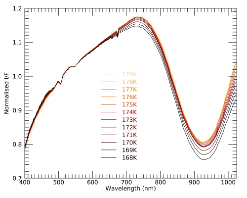
Figure 1 – Median spectral variations observed for each CCD temperature recorded during the VH2 mission phase (normalized at 550nm).
- Spectral correction
As in [2], we defined a correction factor for the different mission phases at Vesta, considering their particularities if necessary. This correction factor requires the definition of a reference temperature, at which the spectral response is considered reliable, and a corresponding reference spectrum. A previous analysis of the same effect on Ceres observations [2], revealed a reference CCD temperature of 177K. The correction has been applied on the mission phases during which VIR acquired VIS data. It allows to obtain a globally coherent dataset. Mapping and reliable spectral studies are then possible (see Fig. 2).
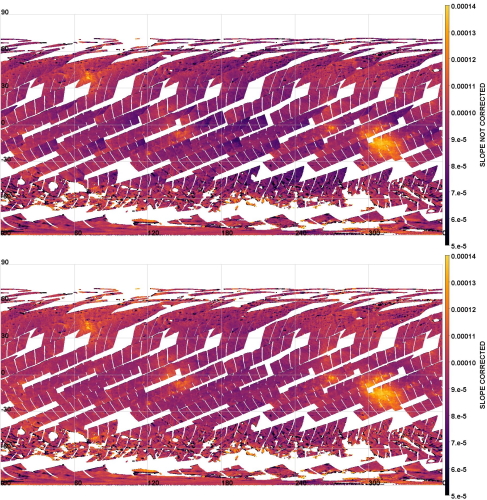
Figure 2 - Map of the spectral slope for the VH2 mission phase before (top) and after (bottom) the correction. The gradient observed, in each sequences, in the top panel vanishes in the bottom panel, after the application of the correction.
- Conclusion
The empirical method developed in [2] has now been applied to the Vesta data acquired by the VIS channel of the VIR spectrometer. This correction is mandatory to carry out reliable analysis of the Vesta surface at global and local scale.
- References
[1] De Sanctis, M. C., Coradini, A., et al. 2011, Space Science Reviews, 163, 329,
[2] Rousseau, B., Raponi, A., Ciarniello, M., et al. 2019, Review of Scientific Instruments, 90,
How to cite: Rousseau, B., De Sanctis, M. C., Ciarniello, M., Raponi, A., Scarica, P., Ammannito, E., Frigeri, A., Carrozzo, F. G., Tosi, F., and Fonte, S.: Dawn/VIR at Vesta: correction of the spectral variations induced by CDD temperature change on the visible channel, Europlanet Science Congress 2020, online, 21 Sep–9 Oct 2020, EPSC2020-116, https://doi.org/10.5194/epsc2020-116, 2020.
Abstract
We aim at retrieving physical and compositional surface properties of the nucleus of comet 67P/Churyumov-Gerasimenko (hereafter 67P) from VIS-IR hyperspectral images (‘cubes’). Here we report on our progress in the geometric modeling and spectral fitting.
Introduction
The measured cubes have been acquired with VIRTIS-M instrument [1] aboard Rosetta. Starting from a digital shape model of 67P [2], the radiance measured by a pixel results from sub-pixel radiance contributions of several shape model facets weighted by the wavelength-dependent spatial point spread function (PSF) of the instrument. Based on a corresponding sub-pixel geometric modeling, we have computed the weighting coefficients and quantified the PSF [3]. The radiance contribution from a single facet can be simulated from physical and compositional parameters defined on this facet, using a photometric model (Hapke or Shkuratov [4,5]). Besides facilitating the consideration of PSF effects, this approach allows us to better approximate the rugged fine-scale topography of 67P that leads to varying observation/illumination/shadowing conditions on sub-pixel scales. Also, the retrieval of parameters common to multiple acquisitions requires a definition of surface parameters bound to the shape model instead of the respective pixel footprints. In this work, we focus on the spectral fitting of entire sets of cubes.
Retrieval algorithm
The Bayesian Multi-Spectrum Retrieval algorithm MSR [6] fits the synthetic spectra to the measured ones by iteratively varying the facet properties. MSR takes into account constraints and Bayesian a priori information on the facet properties (mean values, standard deviations, correlation lengths/times/wavelengths) as well as measurement error information. Moreover, consistency requirements are respected. For instance, for measurements acquired at similar times, there are facet properties (surface roughness, particle size, composition, etc.) that do not change between repeated observations and can be treated and retrieved as common to those observations. To achieve this, MSR regards many measurements of a selected surface region under different illumination and observation conditions, shadowing state, spatial resolution, and at different wavelengths as a single meta-measurement. This is analogous to the meta-measurement formed by measurements at different single wavelengths, called a spectrum.
Preliminary results
At the present stage, MSR is tested to retrieve maps of shape model facet properties from a meta-measurement encompassing tens of VIRTIS-M-cubes, corresponding to the order of a million measured spectra, see Fig. 1.
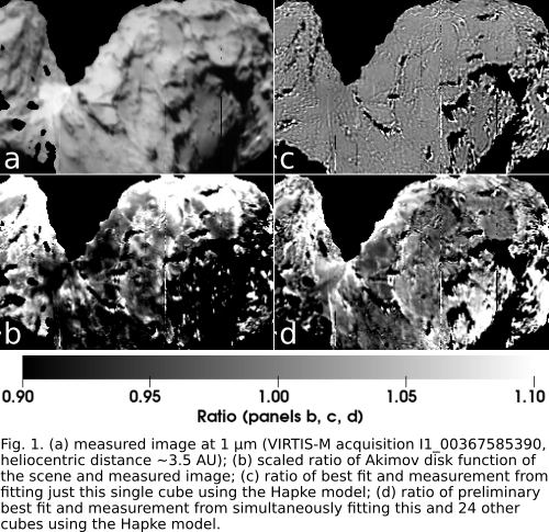
Panel (a) shows a calibrated and pre-processed measured VIRTIS-M cube, represented at 1 µm, mainly showing 67P’s northern hemisphere.
Panel (b) illustrates residual variations when the first-order effect of the complex topography of 67P is removed using the Akimov disk function [5], which describes the photometry of utterly rough surfaces. These residual variations can be due to limits in the applicability of the Akimov disk function or real physical variations in texture or composition. The phase angle (~40°) is too large for substantial opposition effects to show up.
In the case where we fit the entire cube using the Hapke model, panel (c) shows very little residual variations that are mainly associated with local terminators and slight PSF model imprecisions. This image illustrates that our present setup allows us to fit the measurements very accurately when the facet properties can vary freely within the frame of our Bayesian regularization for one cube. For this comparison, we selected as free parameters the single-scattering albedo and phase function asymmetry parameter spectra for two intimately mixed endmembers as properties that are constant over all facets, and the relative abundance of the two endmembers along with the roughness angle and filling factor as properties that can vary between facets.
Finally, panel (d) exhibits moderate residual variations. Here, we fitted a meta-measurement of 25 cubes at various illumination and observation conditions and displayed the one also represented in the other panels. The fitting took about one week on a desktop computer. Now the facet properties cannot vary as freely as for case (c), because simultaneously they also have to be compatible with all other considered cubes. The retrieved facet properties are therefore more well-grounded candidates for the actual surface properties. This panel demonstrates that using information from many hyperspectral images helps to reduce overfitting. We also note that the here utilized set of free parameters is not able to fully capture the spectral variability of the measurements within the frame of this model, pointing to the necessity of additional free parameters, or difficulties of the Hapke model to simultaneously parameterize the different cubes in a consistent way.
At this stage, it is not clear yet, how the retrieved facet properties are related to actual surface properties of 67P. At the meeting we will present different parameter sets that lead to equally well fits and discuss their plausibility. A similar investigation based on the Shkuratov model as well as a detailed error analysis, based on synthetic VIRTIS-M cubes, to investigate interferences between the retrieved and other parameters, are the next steps in this ongoing work. Finally, we expect our approach to be capable of identifying local surface property variations in a physically and mathematically well-grounded way, and we will investigate their correlations with morphologic regions on 67P.
Acknowledgements
We thank the following institutions and agencies for support of this work: Italian Space Agency (ASI, Italy). Centre National d'Etudes Spatiales (CNES, France), DLR (Germany). D.K. acknowledges DFG-grant KA 3757/2-1.
References
[1] Coradini et al. (2007) Space Sci. Rev. 128, 529. [2] Preusker et al. (2017) A&A 607, L1. [3] Kappel et al. (2019) EPSC-DPS 2019, EPSC-DPS2019-456. [4] Hapke (2012) Theory of Reflectance and Emittance Spectroscopy, 2nd edn. (Cambridge University Press). [5] Shkuratov et al. (2011) Planet. Space Sci. 59, 1326. [6] Kappel (2014) J. Quant. Spectrosc. Rad. 133, 153.
How to cite: Kappel, D., Arnold, G., Moroz, L., Raponi, A., Ciarniello, M., Tosi, F., Erard, S., Rousseau, B., Leyrat, C., Filacchione, G., and Capaccioni, F.: Sub-pixel geometric modeling and spectral fitting for Rosetta/VIRTIS-M measurements of the nucleus of comet 67P, Europlanet Science Congress 2020, online, 21 Sep–9 Oct 2020, EPSC2020-226, https://doi.org/10.5194/epsc2020-226, 2020.
We developed a fast algorithm to model a rough planetary surface by means of a statistical multi-facets approach. Consistently with Hapke theory (2012) we model the surface with a distribution of non-spatially resolved facets, being the distribution of their slopes completely described by roughness parameter 𝜃̅.
The parameters in input to model the effect of the surface roughness are the average incidence <i>, emission <e>, and phase <g> angles as inferred from shape model, illumination direction and spacecraft attitude.
Differently from the Hapke model, which is based on analytic relations, here we simulate N facets each with its own viewing geometry (i, e, g), derived from the distribution of slopes (given by 𝜃̅), and from a uniform distribution of rotations of the facets around the axis normal to the average surface. The numerical approach allows us to explore the cases of surfaces with large roughness (𝜃̅>20°) which cannot be described accurately in Hapke model. Once the distributions of i, and e are obtained, significant quantities (e.g. weighted average cosines of illumination and viewing angles), relevant for reflectance modeling, can be calculated as a function of 𝜃̅. Furthermore, the reduction of the scattered power with respect to a smooth surface, produced by the presence of tilted and projected shadows, is computed, similarly to the shadowing function used by the Hapke model.
Our algorithm is capable to model many facets (several thousands) in a short processing time (fractions of a second with a common laptop). The large number of modeled facets ensures a statistically robust result.
This model has two major applications:
- Characterization of the surface roughness by means of best fitting procedures. The correct retrieval of the roughness parameter 𝜃̅ in turn would allow a better retrieval of other quantities relevant for the estimate of additional surface properties (e.g. single scattering albedo, single particle phase function).
- The calculation of the viewing geometry for each facet allows to obtain histograms of relevant parameters for remote sensing applications. As an example, an accurate description of the distribution of the incidence angles on a rough surface is important for thermal modeling applications, since the quantity 4√𝑐𝑜𝑠(ⅈ) in first approximation is proportional to the temperature. This would allow a synergy between thermal emission and reflectance modeling to obtain an estimate of the roughness parameter. Moreover, it would allow the retrieval of a distribution of temperatures along the non-resolved facets. The latter would be important in determining the possible presence and extension of cold trap prone to host ices with direct application to unresolved Permanent Shadowed Regions (PSRs) present on polar regions of Mercury and Moon (Lawrence, 2016).
Here we show a comparison of the output of our computation with the outcomes of the Hapke model, and an application of the present method to characterize the temperature distribution in a rough surface.
Acknowledgments. We thank IAPS (Institute for Space Astrophysics and Planetology) for support of this work.
References:
Hapke B., 2012, Theory of Reflectance and Emittance Spectroscopy, Cambridge Univ. Press
Lawrence D. J., 2016, Journal of Geophysical Research: Planets, 122, pp. 21-52
How to cite: Raponi, A., Ciarniello, M., Filacchione, G., and Capaccioni, F.: Modeling non-resolved rough planetary surfaces by means of a statistical multi-facets approach, Europlanet Science Congress 2020, online, 21 Sep–9 Oct 2020, EPSC2020-761, https://doi.org/10.5194/epsc2020-761, 2020.
The spherical wavelet based on the lifting scheme is introduced for adaptive discrete-ordinate sampling of the radiation fields, particularly, in the radiative transfer computation using iterative schemes. The lifting scheme for wavelet transform is described from an implementation point of view, including the construction of hierarchical geodesic grids on the sphere and wavelet constructions. In addition, we compare the method with the conventional spherical harmonics, numerically investigating the transformation error and efficiency. The transformation matrices are built in the least-squares sense. The results demonstrate the feasibility of using spherical wavelets as an adaptive discrete-ordinate sampling method at the cost of O(N), where N is the number of significant coefficients.
How to cite: Xu, G. and Muinonen, K.: The spherical-wavelet techniques for RT simulation and analysis, Europlanet Science Congress 2020, online, 21 Sep–9 Oct 2020, EPSC2020-981, https://doi.org/10.5194/epsc2020-981, 2020.
We are compiling a service, which will produce almost real-time estimates of the Earth Bond albedo in visual and near-infrared wavelengths using the multi-wavelength images from the NOAA Deep Space Climate Observatory’s (DSCOVR) Earth Polychromatic Imaging Camera (EPIC). The service will be based on the known land and sea surface types of the Earth and the angular distribution models (ADMs) from the Clouds and the Earth’s Radiant Energy System (CERES) project (some details in Ihalainen, M.Sc. thesis, 2019, University of Helsinki, Finland). Instead of applying the CERES ADM albedo estimates as such, we will only use the ADM shapes for different land and sea surface types, but scale them using the corresponding observations from the EPIC camera.
As the EPIC camera will produce imaging of the Earth disk from the L1 point, in about every two hours and in 10 narrow band filters between 317–780 nm, we can follow the temporal changes in the Bond albedo both in short times scales and over longer periods. We will employ a custom-made classifier for cloud coverage over the Earth disk using the 10 bands in the EPIC images to improve the Bond albedo estimation with temporally suitable cloud coverage ADMs over the land or sea surface pixels.
The service will be run automatically in a dedicated server, and will produce the Bond albedo estimates via a public web interface.
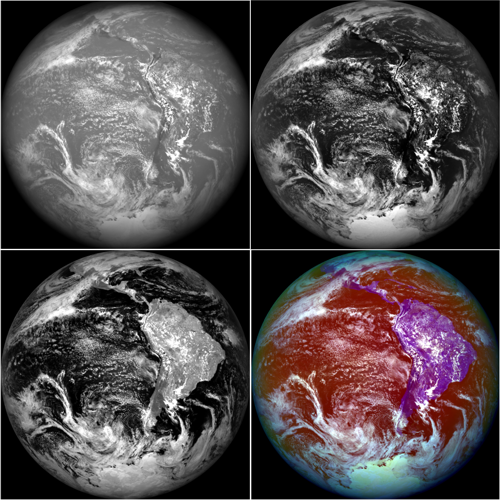
Figure 1. An example image from EPIC camera, taken at Jan. 1st, 2019. The three first images, counting from the top left corner, are gray-scale images at wavelength bands 317 nm, 388 nm, and 780 nm. The fourth image is false-color RGB composite from those channels.
Acknowledgements: Research supported by the Academy of Finland (project 298137).
How to cite: Penttilä, A., Uvarova, E., Vuori, M., Ihalainen, O., and Muinonen, K.: Earth Bond albedo retrieval, Europlanet Science Congress 2020, online, 21 Sep–9 Oct 2020, EPSC2020-749, https://doi.org/10.5194/epsc2020-749, 2020.
The so-called Earth co-orbitals are asteroids that share Earth’s orbit and are potentially linked to leftover material from the formation of the rocky planets. They are difficult to observe from the ground, because of their low conjunction frequency. Here we present light curves of a number of co-orbitals successfully observed during very narrow visibility periods when they approach the Earth. We used the FoReRo2 instrument attached on the 2-m RCC telescope at the Bulgarian National Astronomical Observatory - Rozhen. The figure shows the light curve of (418849) 2008 WM64, which has a semi-major axis a=1.005 AU, an orbital period of 1.01 yr and absolute magnitude H=20.6.
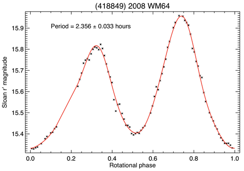
Knowing their spin rate and determining the magnitude of the YORP and Yarkovsky effects we can make inferences about their creation (YORP-induced fission of a parent body) and their past orbital evolution.
Acknowledgements
Work reported here was supported via grant ST/R000573/1 from the UK Science and Technology Facilities Council (STFC). Astronomical research at the Armagh Observatory and Planetarium is grant-aided by the Northern Ireland Department for Communities (DfC).
How to cite: Borisov, G., Christou, A., Bagnulo, S., Cellino, A., and Dell'Oro, A.: Light curves and spin rates of Earth co-orbital asteroids, Europlanet Science Congress 2020, online, 21 Sep–9 Oct 2020, EPSC2020-324, https://doi.org/10.5194/epsc2020-324, 2020.
1. Introduction
Studying Very Small Asteroids (VSAs, effective diameter <150 m) is important for understanding the structure and evolution of asteroids and some non-gravitational effects (YORP and Yarkovsky effects). VSAs originate from collisions or rotational disintegration of larger bodies, which are the so-called rubble pile asteroids. Because VSAs are monoliths, they can have shorter rotation periods than the spin barier (P<2.2 h), which limits the rotation rates of rubble piles.
Due to their small sizes VSAs are usually observed as Near-Earth Asteroids (NEAs), during their close approaches to Earth. At that time they pose an observational challenge due to fast movement in te sky.
2015 KW120 is NEA belong to Apollo group. It was discovered on 24 May 2015 by Catalina Sky Survey (MPEC 2015-K99). At the night of our observations (29 May), it was closest to the Earth at 1.1 Earth-Moon distance and its magnitude (according to the MPC) was V=15.6.
2. Observations and data reduction
Observations were performed with a 0.7-m robotic RBT/PST2 telescope at Winer Observatory in Arizona, with the Andor iXon3 888 CCD camera, which has a field of view (FoV) 10' x 10'. We used a broadband filter L ("luminosity", transmission 370-700 nm), which can be thought of as a sum of the g and r SDSS bands. Each CCD frame was exposed for 15 seconds. Data were calibrated for bias and flat field.
As the proper motion of 2015 KW120 was very high (370 arcsec/min), the telescope followed the asteroid to keep it in the FoV and to maximize the S/N. In this way, the image of the asteroid remained round on the CCD frame, and the images of the stars were trailed (Fig. 1). Instrumental magnitude measurements for the asteroid were made using the standard aperture photometry method (Fig. 2).
Usually the changes of the atmosphere transparency affect a lightcurve. This can be prevented by using comparison stars. But in our case, with a fast-moving asteroid, we came across two issues:
1) Long trails of stars in the CCD frame, for which the appropriate aperture shape should be used (an ellipse or better a pill[4]). We could not do automatic photometry of such fast changing position trails using Starlink package[1]. (The aperture position would have to be manually specified.)
2) At this speed, potential comparison stars leave the FoV very quickly. Our estimates assume that we would need about 90 stars to cover the entire observation.
Both reasons make the differential photometry in this case very laborious. Fortunately, the night was photometric and the collected data are of good quality, allowing for accurate determination of the rotation period.
3. Rotation period
We determined the rotation period by folding curves with the least squares fit of the Fourier series. The algorithm of our program was described in [5].
We obtained 4 probable solutions for the period: P1, P2, P3 and P4 (see Fig. 3). The most likely is P2=0.1358 h (see solution P2 in Fig 3 and composite curve for P2 solution in Fig 4.). The two maxima and two minima of the brightness of this solution are typical for the commonly accepted triaxial ellipsoid approximation of the shape of most asteroids. We also analyzed the remaining 3 solutions in terms of the probability of a curve dominated by a given Fourier harmonic at a given peak-to-peak amplitude and the solar phase angle. For this, we used tables from [2]. As observations were made at the phase angle of 64-74° and the amplitude is about 1.35 mag (measured from the Fourier fit curve), other solutions are very unlikely.
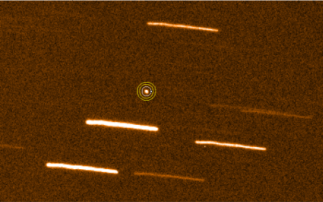
Fig. 1. A fragment of an example CCD frame, showing the trailed stars. The 2015 KW120 asteroid image is marked with a yellow aperture.
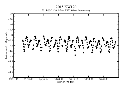
Fig. 2. Lightcurve of 2015 KW120
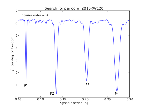
Fig. 3. Search period results showing a range of trial periods and the corresponding χ2 per degree of freedom. There are four possible solutions, marked by P1,P2,P3 and P4
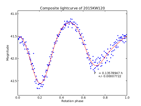
Fig. 4. Composite lightcurve of 2015 KW120 for the most probable rotation period P2.
4. The asteroid location in the period-diameter plot
The effective diameter can be determined from a standard equation given in [3]:
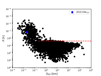
where: pV means the geometric albedo of the asteroid surface in the V band and H means absolute magnitude. The value of H=26 mag was taken from the Minor Planet Center. The albedo is not known for this asteroid, so we assumed pV=0.2 (this value is used in the Asteroid Lightcurve Database (LCDB) [6] for NEAs). Hence, we received D=19 m. The asteroid location in the PvsDeff plot is marked with a blue square in Figure 5. The asteroid definitely exceeds the spin barrier and is small in size, hence we conclude that it has a monolithic structure.
References
5. Summary
We observed 2015 KW120 asteroid, determined the rotation period P=0.1358±0.0001 h (8.147±0.006 min), and the amplitude peak-to-peak A=1.35 mag. Based on the location of the asteroid on the logP-logDeff chart, we conclude that the asteroid is a rapidly rotating monolith. In the near future, we are going to publish the results for other VSAs and also continue to observe objects of this type.
References
[1] Butkiewicz-Bąk et al. (2017) MNRAS 470, 1314-1320
[2] Currie et al. (2014) Astronomical Society of the Pacific Conference Series 485, 391
[3] Fowler and Chillemi (1992) Phillips Laboratory, Hanscom AF Base, MA, 17--43
[4] Fraser et al. (2016) The Astronomical Journal 151, 151-158
[5] Kwiatkowski et al. (2010) A&A 509, A94
[6] Warner et al. (2009) Icarus 202, 134
How to cite: Koleńczuk, P., Kwiatkowski, T., and Kamiński, K.: Photometry of super fast rotating, near-Earth asteroid 2015 KW120, Europlanet Science Congress 2020, online, 21 Sep–9 Oct 2020, EPSC2020-809, https://doi.org/10.5194/epsc2020-809, 2020.
Abstract
The so-called “primordial family”, is a recently discovered collisional family [1] that could be as old as the Solar system. It contains low-albedo asteroids and is located in the inner Main Belt. This family was identified by the V-shape technique [2] and is estimated to be at least 4 Gyr old, meaning that occurred before the giant planet instability [3]. Asteroids 2768 Gorky (1972 RX3) and 9086 (1995 SA3) are members of the primordial family and have been observed in order to determine their rotational period, spin pole and shape, which will give insights about their membership and the family evolution. The photometric data are obtained mainly by the University of Athens Observatory (UOAO) [4]. Models of the asteroids are derived by the lightcurve inversion method, which is stored in the Database of Asteroid Models from Inversion Techniques (DAMIT) [5].
1. Introduction
The so-called primordial family formed by an impact event 4 Gyr ago or even earlier, i.e. before the giant planet instability [3]. The identification of the primordial family has been done by using the V-shape technique [2]. The V-shape in (α,1/D) space is occurred due to the thermal Yarkovsky effect [6, 7, 2], where prograde-rotating asteroids drifting outwards and retrograde ones inward. As only the inward side of the V-shape of the primordial family is well defined, the members should have retrograde spin. Otherwise, the membership of asteroids with prograde spin could be disputed or the contradicting spin sense could be due to YORP cycles or a collision or a close encounter with other asteroid [8, 9]. Thus, it is essential to observe thoroughly the asteroids belonging to the primordial family, in order to determine their rotational state and shape.
2. Observations
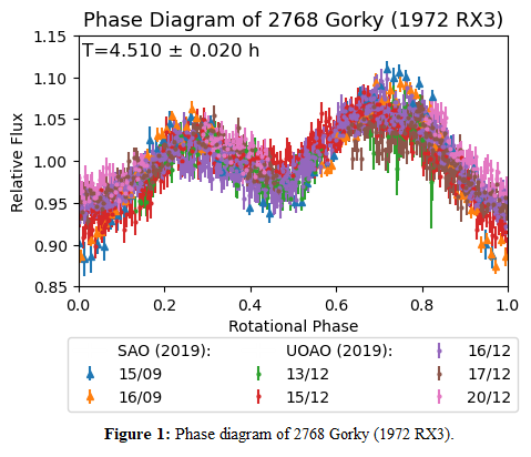
Asteroid 2768 Gorky (1972 RX3) is member of the primordial asteroid family of the inner main belt [1]. Its rotational period is 4.507 ± 0.010 h [10], while its spin pole and shape remain unknown. Observations from Sopot Astronomy Observatory (SAO) for 2 nights in September 2019, in phase angle of 32º, are available in Asteroid Lightcurve Photometry Database (ALCDEF)[11] and present a period of 4.445 ± 0.003 h [12]. On the Observatoire de Genève website of R. Behrend [13] rotational period of the asteroid was reported to be 4.5118 ± 0.0007 h. Asteroid 2768 Gorky (1972 RX3) has been observed from UOAO for 5 nights in December 2019, in phase angles between 10º to 14º.
Asteroid 9086 (1995 SA3) is member of the primordial asteroid family in the inner main belt [1]. Its rotational period, spin pole and shape remain unknown. UOAO has been observed this asteroid for 22 nights from October to November 2019, in phase angle ranging between 4º to 22º.
3. Methodology and Preliminary Results
Differential photometry of the asteroid has been obtained for each sky field. All images were dark and flat-field corrected and unguided. The measured values are in magnitudes and have been transformed properly in relative flux. The determination of the rotational period of the two asteroids and the estimation of the spin pole and shape of 2768 Gorky (1972) has been carried out through the lightcurve inversion method stored in DAMIT [5].
3.1 Asteroid 2768 Gorky (1972 RX3)
The lightcurve of asteroid 2768 Gorky (1972 RX3) present a low amplitude of ~0.1 mag (or ~0.1 intensity units), as Figure 1 shows. Generating 50 random spin poles as initial input for DAMIT software, the results have the distribution presented in Figure 2. The plot in this figure constrains the possible spin poles of the asteroid, while the χ2 value and the dark facet percentage should have the lowest value.

3.2 Asteroid 9086 (1995 SA3)
The lightcurve of asteroid 9086 (1995 SA3) present also a low amplitude of ~ 0.2 mag (or ~0.2 intensity units). The low brightness of the object in combination with the low amplitude of its lightcurve render the detection of its periodicity difficult, due to the background noise. In order to address this problem, the exposures of each night were combined in packs of 3, in order to increase the S/N and make the detection of light variation more prominent. The resulted period spectrum from DAMIT is presenting in Figure 3.

4. Summary and Conclusions
The rotational period of 2768 Gorky (1972 RX3) has been calculated as 4.510 ± 0.020 h, in agreement with the literature. The spin pole is not defined well enough. It is needed observations from more than one apparition for more robust results. Asteroid 9086 (1995 SA3), despite the extensive observations, does not present a clear lightcurve, as a result to have not unique solution in the period.
5. Further work
The determination of asteroids’ rotational state and shape requires observations from more than one apparition. Alternatively, combing the already ground based with sparse data from sky surveys or space-borne could also drive to unique solutions.
Acknowledgements
We would to acknowledge Dr. Hanus J. for his valuable help and advices for the lightcurve analysis that performed.
References
[1] Delbo, M. et al. (2017). Science, 357, 1026-1029.
[2] Bolin, B. T. et al. (2017). Icarus, 282, 290-312.
[3] Tsiganis, K., et al. (2005). Nature, 435(7041), 459-461.
[4] Gazeas, K. (2016). Revista Mexicana de Astronomía y Astrofísica, 48, 22-23.
[5] Ďurech, J. et al. (2010). Astronomy & Astrophysics, 513, A46. (DAMIT’s website: astro.troja.mff.cuni.cz)
[6] Milani, A. et al. (2014). Icarus, 239, 46-73.
[7] Spoto, F. et al. (2015). Icarus, 257, 275-289.
[8] Carruba, V. et al. (2013). Monthly Notices of the Royal Astronomical Society, 433(3), 2075-2096.
[9] Delisle, J. B., & Laskar, J. (2012). Astronomy & Astrophysics, 540, A118.
[10] Pray, D. P. et al. (2008). Minor Planet Bulletin, 35, 34-36.
[11] Asteroid Lightcurve Photometry Database (ALCDEF)’s website: alcdef.org
[12] Benishek, V. (2020). Minor Planet Bulletin, 47(1), 75-83.
[13] Observatoire de Genève, Website of R. Behrend: obswww.unige.ch/~behrend
How to cite: Athanasopoulos, D., Gazeas, K., and Delbo, M.: Preliminary results on the photometric study of two primordial family asteroids, Europlanet Science Congress 2020, online, 21 Sep–9 Oct 2020, EPSC2020-733, https://doi.org/10.5194/epsc2020-733, 2020.
The brightness of minor bodies depends, among other things, on their phase curves. Furthermore, the absolute magnitude, of a minor body is obtained from these curves, requiring observations at different phase angles, thus being impossible to obtain in a single observing night. Large photometric surveys help due to serendipitous observations of minor bodies in different epochs and phase angles.
Multiple wavelength phase curves have not been thoroughly explored yet, in particular, the possibility of obtaining photo-spectra (a very low resolving-power spectrum) at zero phase angle, i.e., not affected by phase coloring. In this presentation, we show preliminary results of multi-wavelength phase curves for over a thousand objects obtained using data from the SLOAN moving object catalog and discuss the statistical properties of the sample.
How to cite: Alvarez-Candal, A., Campo Bagatin, A., Benavidez, P., and Santana-Ros, T.: Multi-wavelength phase curves of minor bodies, Europlanet Science Congress 2020, online, 21 Sep–9 Oct 2020, EPSC2020-616, https://doi.org/10.5194/epsc2020-616, 2020.
Abstract
We apply the statistical lightcurve inversion method developed by Muinonen et al. (2020, convex inversion in magnitude space CIM) to re-analyze the photometric data of (346) Hermentaria. As a main goal, we compare the results derived by the CIM and original convex inversion method in flux space (CIF) provided by Kaasalainen & Torppa (2001) and Kaasalainen et al. (2001). The comparison concerns the solutions of spin and shape parameters.
1. Introduction
The idea to invert 3-D shapes of asteroids from their brightness variations can be traced to 1906 (Russell 1906). Now, several methods have been established to invert the shape of asteroids, the shape models range from triaxial ellipsoids to convex, and even non-convex shapes. Kaasalainen et al. (1992a,b) and Lamberg (1993) suggested a way to invert the convex shape of an asteroid by using the Gaussian surface density. Kaasalainen & Torppa (2001) and Kaasalainen et al. (2001) implemented the idea by the Levenberg-Marquardt algorithm.
Now, statistical techniques have been introduced into the photometry inversions of asteroids, e. g., a genetic algorithm (Cellino et al. 2015) and a Markov-chain Monte Carlo approach (MCMC, Muinonen et al. 2015). Wang et al. (2015b,a) presented a virtual observation method to figure out the uncertainties of parameters due to the observational uncertainties. Muinonen et al. (2020) developed a full statistical MCMC algorithm in the convex inversion of asteroids in the magnitude space (CIM), and gives a way to assess the uncertainties of spin parameters and convex shape parameters.
We re-analyse the photometric data of (346) Hermentaria with CIM and CIF algorithms, and show the main differences of the results in the derivation of the convex shapes.
2. Convex inversion with Bayesian inference
The brightness model used in the CIM (Muninonen et a l. 2020)) involves a convex shape represented with the Gaussian surface density and the Lommel-Seeliger scattering law. In the CIM, the free parameters are the spin parameters, shape parameters, geometric albedo, and two parameters of the H,G1,G2 phase function. As for constructing the convex shape from its Gaussian surface density, Muinonen et al. (2020) developed a computationally easier, stochastic optimization metod.
3. Results and discussion
In total, 23 lightcurves of (346) Hermentaria on 4 apparitions are involved. 10 light curves are from the APC database (Lagerkvist et al. 1993) and rest of the lightcurves are ours observations. Based on these data, we performed the shape inversion with the CIM and CIF methods. As only relative intensities are involved, the parameters of the H G1 G2 phase function in the CIM and the scattering parameters a, k,d and c in the CIF are not fitted. Table 1 list the derived spin parameters. Figure 1 shows the lightcurves fits for the case of the pole 2 solution.
Table 1. Spin parameters of Hermentaria
| Method |
Pole 1 (Ecliptic frame of J2000.0 ) |
Pole 2 (Ecliptic frame of J2000.0 ) |
Peroid (h) Pole 1, Pole 2 |
| CIF |
(133o.0,+17o.2) |
(319o.5,+16o.8) |
17.790043, 17.790039 |
| CIM |
(133o.8,+09o.6) |
(321o.9,+17o.2) |
17.790016, 17.790097 |


Figure 1. Lightcurves of Hermentaria (black circles) with the CIM and CIF model intensities ( red crosses and blue pluses respectively).
The CIM gives a consistent result on spin parameters. From Figure 1, the modeled lightcurves with the CIF fit well to the features. We think this is partly due to the fact that we use a lower degree of spherical harmonics in the CIM and partly due to the differing model for the observational uncertainties.
The theory by Minkowski (1903) provides a way to construct the three-dimensional shape of an object from its Gaussian surface density G. According to Minkowski, Muinonen et al.(2020) developed a stochastic optimization method to construct convex shape. Figure 2 shows the convex shapes of Hermentaria derived by the two methods.

Figure 2. Convex shapes of Hermentaria corresponding to Pole 2 solution: the CIM (left) and CIF solutions (right)
We have also compared the 3-D shapes constructed by the CIM and the CIF using the same Gaussian surface density originally derived by the CIM. Figure 3 shows the CIM and CIF results and by visual inspection, the results are very close to one another.

Figure 3 Convex shapes of Hermentaria corresponding to the same Gaussian surface density:
the CIF (left) and CIM reconstructions (right).
4. Summary
We applied the statistical convex inversion method (Muninonen et al. 2020) to analyze the photometric data of Hermentaria. The best-fit solution of the spin parameters and shape as well as the uncertainties of the estimated parameters can be derived.
We compared the results to that of the CIF and found that the spin parameters are consistent with one another. The Gaussian surface density derived by the two methods is slightly different which leads to slightly different convex shapes.
For validating the new shape reconstruction method in Muinonen et al. (2020), we compared the shape derived by the methods of Kaasalainen tel al.(2001) and Muinonen et al. (2020) from the same Gaussian surface density, and found them to be similar.
References
Cellino, A., Hestroffer, D., Tanga, P., Mottola, S., & Dell’Oro, A. 2009, A&A, 506, 935
Cellino, A., Muinonen, K., Hestroffer, D., & Carbognani, A. 2015, PSS, 118, 221
Kaasalainen, M., Lamberg, L., & Lumme, K. 1992a, A&A, 259, 333
Kaasalainen, M., Lamberg, L., Lumme, K., & Bowell, E. 1992b, A&A, 259, 318
Kaasalainen, M. & Torppa, J. 2001a, Icarus, 153, 24
Kaasalainen, M., Torppa, J., & Muinonen, K. 2001b, Icarus, 153, 37
Lagerkvist, C.-I., Erikson, A., Debehogne, H., et al. 1995, A&A Supplement Series, 113, 115
Lamberg, L. 1993, Ph.D. thesis, University of Helsinki, Finland, vol. 315L
Minkowski, H. 1903, Mathematische Annalen, 57, 447
Muinonen, K. & Lumme, K. 2015a, A&A, 584, A23
Muinonen, K., Wilkman, O., Cellino, A., Wang, X., & Wang, Y. 2015b, PSS, 118, 227
Muinonen ,K., Torppa, J., Wang, X.-B., Cellino,A., Penttilä , A., 2020, submited to A&A, in revised
Russell, H. N. 1906, Astrophys J, 24, 1
Wang, X., Muinonen, K., & Wang, Y. 2015a, PSS, 118, 242
Wang, X., Muinonen, K., Wang, Y., et al. 2015b, A&A, 581, A55
How to cite: Wang, X., Muinonen, K., and Cellino, A.: Photometric analysis for asteroid (346) Hermentaria: comparison of inverse methods, Europlanet Science Congress 2020, online, 21 Sep–9 Oct 2020, EPSC2020-490, https://doi.org/10.5194/epsc2020-490, 2020.
Abundance and speciation of Fe play an important role in meteorite classification. Ordinary chondrites, for example, are grouped based on their Fe content and speciation into H chondrites (H for high total Fe and high metal content), L chondrites (L for low total Fe) and LL chondrites (low total Fe, low metal). In differentiated bodies metallic Fe partitions into the core while oxidized Fe stay in the mantle. Mössbauer spectroscopy is a powerful tool to determine Fe-bearing mineral phases and Fe oxidation states, and to quantify the distribution of Fe between mineral phases and oxidation states. The miniaturized Mössbauer spectrometer MIMOS II is set up in backscattering geometry and thus enables non-destructive measurements of whole rock samples [1]. Creating a database of Mössbauer analyses of meteorites reported in the literature and from our own analyses with MIMOS II, we are investigating whether Mössbauer spectral information allows to distinguish between meteorite groups. It could then be used alongside other non-destructive techniques used for meteorite classification such as magnetic susceptibility measurements [2] and elemental analysis with portable X-Ray Fluorescence (XRF) spectrometers [3].
Mössbauer parameters were assembled from [4-6] and from measurements of meteorites loaned from the collections of National Museums Scotland (NMS). Literature data were obtained by measuring pulverized bulk rock samples in transmission geometry. The NMS meteorites were analysed with a MIMOS II instrument [1] at the Mössbauer Spectroscopy laboratory for Earth and Environment (MoSEE) at the University of Stirling. MIMOS II has a 1.4 cm diameter circular field of view, and we measured interior meteorite surfaces free of fusion crust.
In Fig. 1 we compare ordinary chondrites (OCs) with several achondrite groups where Fe is distributed between Fe(II) in olivine and Fe(0) in the metallic phase (the Fe-Ni alloy kamacite). OC H, L, and LL data are from [4], ureilite data are from [5]. Howardite, eucrite and diogenites (HEDs) have been measured for this work. A set of paired stony meteorites have been investigated with a MIMOS II on board the Mars Exploration Rover Opportunity at Meridiani Planum on Mars [6]. On the basis of their chemical composition they are similar to HEDs but have a higher metal content, which would be consistent with the silicate fraction of mesosiderites [6]. They are labeled as HED/MES in Fig. 1.
 Fig. 1
For the plot in Fig. 1 we have made the assumption that any Fe(III) measured stems from terrestrial weathering of most likely the metal phase. We have therefore added that Fe fraction to the kamacite metal fraction. This plot allows for a clear distinction between H and L, and H and LL groups. L and LL groups overlap and cannot be distinguished. However, this complements magnetic susceptibility measurements, which are able to clearly distinguish L and LL groups, but the data for L and H groups overlap [4] A combination of Mössbauer an magnetic susceptibility is therefore able to resolve the groups unambiguously. The two LL chondrites plotting amongst the H chondrites are so severely weathered that olivine was also weathered and contributed Fe to the Fe(III) weathering phases.
Ureilites, a group of primitive achondrites, plot in an area distinct from the H, L and LL OCs. There are two outliers. One near a kamacite + Fe(III) value of ~80% is so severely weathered that all kamacite has been converted to Fe(III), and the Fe(III) fraction likely also contains a significant fraction of Fe from weathered olivine. The other lies near a kamacite + Fe(III) value of ~42% and has an unusually high amount of Fe(II) associated with pyroxene rather than olivine.
The HED/MES meteorites found on Mars plot close to the L and LL OC groups and do not overlap with the HEDs. HEDs generally contain little olivine and metal, if any, and therefore plot close to the origin of the diagram. Excursions to higher kamacite + Fe(III) values larger than 10% are a result of substantial terrestrial weathering. We need to obtain Mössbauer spectra from mesosiderite silicate fractions to establish a grouping with the HED/MES specimens. The HEDs all plotting on the X-axis highlight that different parameters need to be plotted to compare, for example, more evolved stony achondrite groups that do not contain any metallic Fe, and meteorite groups that do not contain olivine.
Mössbauer spectroscopy has not been applied systematically to meteorites so far. As a result, Mössbauer data are not available for all meteorite groups or lack a statistically significant number of analyses of different specimens from each group. This work is therefore ongoing. We could show that certain meteorite groups can be distinguished on the basis of Mössbauer data. Some ambiguities can be resolved by applying other non-destructive techniques, e.g. magnetic susceptibility measurements or XRF. Mössbauer spectroscopy, magnetic susceptibility, and XRF are available in portable form and can be applied in the field or in situ on the surface of asteroids during similar missions, where they would provide an unequivocal link between parent body and the relevant meteorite group. Because these methods are non-destructive, they can also be applied to the small and invaluable sample volumes that will be returned from asteroids in ongoing missions such as the Japanese Hayabusa2 and NASA’s Osiris Rex.
References
[1] Klingelhöfer, G. et al.: Athena MIMOS II Mössbauer spectrometer investigation. Journal of Geophysical Research 108, 8067, doi:10.1029/2003JE002138, 2003.
[2] Rochette, P., et al..: Magnetic classification of stony meteorites: 1. Ordinary chondrites. Meteoritics & Planetary Science, Vol. 38, pp. 251-268, 2003.
[3] Zurfluh, F.J. et al.: Evaluation of the utility of handheld XRF in meteoritics. X-Ray Spectrometry, Vol. 40, pp. 449–463, 2011.
[4] Righter, K. et al.: Non-destructive classification approaches for equilibrated ordinary chondrites, Meteoritics and Planetary Science, Vol. 48(s1), 5232, 2013.
[5] Burns, R.G., and Martinez, S.L.: Mössbauer Spectra of Olivine-rich Achondrites: Evidence for Preterrestrial Redox Reactions. Proceedings of Lunar and Planetary Science, Vol. 21, pp. 331-340.
[6] Schröder, C. et al.: Properties and distribution of paired candidate stony meteorites at Meridiani Planum, Mars. Journal of Geophysical Research 115, E00F09, doi:10.1029/2010JE003616, 2010.
How to cite: Schröder, C., Fay, A., and Davidson, P.: Non-destructive meteorite classification using Mössbauer spectroscopy, Europlanet Science Congress 2020, online, 21 Sep–9 Oct 2020, EPSC2020-478, https://doi.org/10.5194/epsc2020-478, 2020.
Context
In the past about 10-15 years ground- and space-based observations of asteroids, results from space missions, and new efforts in laboratory and modeling work has advanced significantly, providing further and new data in many domains. On basis of these data, including much more volume and mass estimates, and from that density averages per taxonomic class, new statistical approaches revealed further structures in the asteroid belt and population, with implication on the description of the current and former state of the Solar System (DeMeo & Carry 2013). They suggest a more dynamic evolution of it (supporting the Grand Tack and Nice models) than thought before, but also rises new questions (see,e.g., DeMeo & Carry 2014, Michel et al. 2015).
Motivation and Aim
Size (volume), mass, density, and macro porosity are important physical properties for our understanding of the internal structure and morpholgy of asteroids (Scheeres et al. 2015). Though, we yet have density estimates for only some hundred objects (Carry 2012, this work), and only about 1/3 of them have a relative accuracy better than 20%. With very few exceptions, bulk densities are calculated from individual size and mass estimates, which themselves are derived using different methods. The number of density estimates is limited by the number of available mass estimates. Moreover, the relative accuracy of mass estimates is in many cases lower compared to that of size estimates, and, sometimes even incompatible between different methods within the formal uncertainties. The situation for sizes is generally better in terms of quantity, but also accuracy. Nevertheless even these comparable small relative errors of volume estimates can result in significant uncertainties of the derived density because of the relation ρ ~ D-3, were D is the volume-equivalent diameter. Comparing results derived by different methods (for both properties mass and volume), constraint by realistic density ranges, can reveal limitations and biases of the individual methods.
Up to now, no machine-readable, easy to use and open-access data collection was available. Purpose of SiMDA (Size, Mass and Density of Asteroids) is not only to serve as an up-to-date and complete collection of size and mass estimates, providing researchers with ready to use data, but also to support some visualization and interactive handling of the data addressing the issues mentioned before.
Data Sets
Starting point for this work was the data compilation by Carry (2012), with ~1000 mass and ~1500 volume estimates. These estimates were evaluated for each object (in most cases averaged), in order to derive a single value for the size, mass and bulk density for finally 287 small bodies (a dozen comets included).
In the work presented here, all data and references given in Carry (2012) were verified by examination of the original work (where possible) and completed if necessary, and then added to the data base. For the time after that date (2011/2012), the literature (and the web) was and is regularly searched for publications of mass and / or size estimates or any direct density measurements, which are then added to the SiMDA data base. This is of course an ongoing process. To name some examples: further volume data will become available due to continued light-curve and stellar occultation observations (both domains with large contributions by amateur astronomers), and by using combined-data asteroid shape and size modeling (see, e.g. Hanuš et al. 2017). The observation of asteroids by Gaia will allow to determine the mass of about 100 asteroids with a relative accuracy better than 50% (Mouret et al. 2008), and planetary ephemerides (INPOP, JPL DE) will provide new mass estimates on a regular basis as well. Currently (May 2020) ~1750 mass and ~4000 diameter estimates for ~425 objects are archived.
Implementation and Usage
SiMDA is implemented as web application, written in Python (https://www.python.org), and using Django (https://www.djangoproject.com) as framework. Data are stored in a SQLite (https://www.sqlite.org) data base. Plotly (https://www.plotly.com) provides visualization. Tabula (https://tabula.technology/) and Excalibur (https://excalibur-py.readthedocs.io/en/master/) is used to extract tabular data from PDFs, where necessary.
SiMDA (https://kretlow.de/simda) provides size and mass estimates and the references of the original works. These data are completed by taxonomic information, if available. The web user interface allows to search for an object or to select it from a list. All available size and mass data for the selected object are displayed in tabular form and visualized as scatter plot. Average values and a derived bulk density are calculated on the fly, including their standard errors. It is possible to interactively change this calculations, i.e. to select / deselect individual size and / or mass estimates and to update the numerical results and plots.
The second main feature is to provide a data catalog for all objects. A single ‘best’ value for size, mass and the bulk density is calculated and the resulting catalog can be downloaded in different formats for own research and further processing.
References
B. Carry, 2012. Density of asteroids. Planetary and Space Science, Volume 73, p. 98-118.
F.E. DeMeo, B. Carry, 2013. The taxonomic distribution of asteroids from multi-filter all-sky photometric surveys. Icarus, Volume 226, Issue 1, p. 723-741.
F.E. DeMeo, B. Carry, 2014. Solar System evolution from compositional mapping of the asteroid belt. Nature, Volume 505, Issue 7485, p. 629-634.
J. Hanuš, M. Viikinkoski, F. Marchis, J. Ďurech, M. Kaasalainen, M. Delbo', D. Herald, E. Frappa, T. Hayamizu, S. Kerr, S. Preston, B. Timerson, D. Dunham, and J. Talbot, 2017. Volumes and bulk densities of forty asteroids from ADAM shape modeling. Astronomy & Astrophysics, Volume 601, A114, 41 pp.
P. Michel, F.E. DeMeo, and W.F. Bottke, 2015. Asteroids: Recent Advances and New Perspectives. In "Asteroids IV" (P. Michel et al., Eds.). pp. 3-10. Univ. of Arizone, Tucson.
S. Mouret, D. Hestroffer, and F. Mignard, 2008. Asteroid mass determination with the Gaia mission. A simulation of the expected precisions. Planetary and Space Science, Volume 56, Issue 14, p. 1819-1822.
D. J. Scheeres, D. Britt, B. Carry, and K.A. Holsapple, 2015. Asteroid Interiors and Morphology. In "Asteroids IV" (P. Michel et al., Eds.). pp. 3-10. Univ. of Arizone, Tucson.
How to cite: Kretlow, M.: Size, Mass and Density of Asteroids (SiMDA) - A Web Based Archive and Data Service, Europlanet Science Congress 2020, online, 21 Sep–9 Oct 2020, EPSC2020-690, https://doi.org/10.5194/epsc2020-690, 2020.
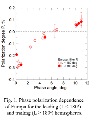
Particles of water ice are an integral part of many objects of the solar system - from the Moon and comets to the satellites of giant planets. For example, Europa is the smallest of the four Galilean moons orbiting Jupiter, and has a water-ice crust on surface. To study the chemical and physical properties of Europa’s ice crust, both photopolarimetrical observations and computer simulation of light scattering are required. Fig. 1 represents the new most accurate the phase curve of polarization of Europa in the filter R, obtained in 2018-2019 at the 2.6 - m telescope of the Crimean Astrophysical Observatory and 2-m RCC telescope of the Pik Terskol Observatory.
But for proper interpretation of observational data we should have information about the shape of the ice particles. Transition between amorphous and crystalline water ice phase can dramatically change the photopolarimetrical properties.
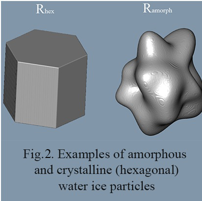
We carried out the computer simulation of light scattering by hexagonal ice crystals and amorphous ice particles (see fig. 2).
Shape of hexagonal crystals of water ice is described by Niels Bjerrum [1]. As a model of amorphous ice, random Gaussian particles were chosen, described in detail in [2].
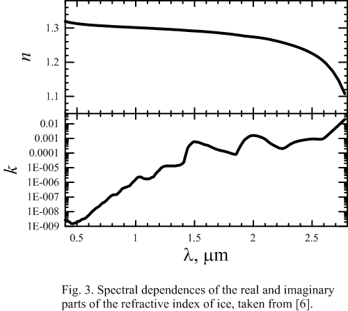
The particles are characterized by a size parameter X = 2πR/λ, where λ is the wavelength of the incident light, and R is the radius of sphere of equal volume. Here we consider a wide range of wavelengths - from 0.4 μm to 2.8 μm.
To calculate the light scattering properties of individual scattering particles the T-matrix method is often used [3]. Our calculations were performed by modifying the T-matrix method (the so-called Sh-matrices method, or the shape matrices method, described in [4, 5]).
Particles can be characterized by a complex refractive index m0 = n + i∙k. The spectral dependence of the refractive index (both real and imaginary parts) of ice particles on the wavelength is shown in Fig. 3. Data taken from [6].
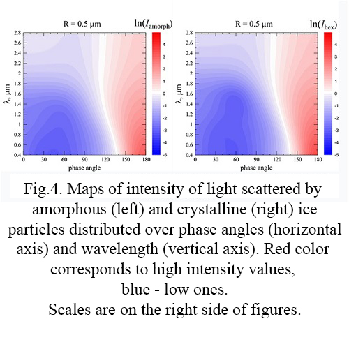
We calculated the intensity of light scattered by crystalline and amorphous ice particles at particles size R = 0.5µm. The results of the calculations are shown on figure 4. On this figure you can see the maps of ln(I), where intensity depends on both phase angle and wavelength of scattered light.
The linear polarization of scattered light by is characterized by the following equation:
 (1)
(1)
where and are the intensity of perpendicular and parallel components of scattered light with respect to the scattering plane.
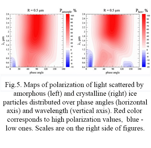
Figure 5 shows maps of the degree of linear polarization of amorphous and crystalline ice particles. The X axis corresponds to the scattering angle values, and the Y axis - to the wavelengths.
The figure shows a noticeable difference between the crystalline and amorphous structures. In the case of a crystalline structure, the branch of negative polarization is generally deeper and exists in a wider range of wavelengths.
For the most visual demonstration of differences, Figure 6 is shown, on which maps of the difference in intensity and degree of linear polarization of light scattered by crystalline and amorphous ice are built.
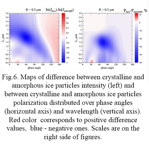
Based on figures, we can draw the following conclusions:
References
How to cite: Petrov, D., Savushkin, A., Zhuzhulina, E., Kiselev, N., Rosenbush, V., and Karpov, N.: The effect of crystallization on the photopolarimetrical properties of Europa’s ice crust, Europlanet Science Congress 2020, online, 21 Sep–9 Oct 2020, EPSC2020-532, https://doi.org/10.5194/epsc2020-532, 2020.
1. INTRODUCTION
In planetary sciences, rotational motion induced by interactions between solar system bodies and electromagnetic radiation is often attributed to the the Yarkovsky-O’Keefe-Radzievskii-Paddack (YORP) effect (Rubincam 2000). The YORP effect is related to anisotropic momentum exchange between the body and absorbed, reflected, or emitted photons relative to the body center of mass. For smaller particles, radiative torques (commonly referred to as RATs, see, e.g. Lazarian & Hoang, 2007) emerge from direct exchange of angular momentum in the scattering interaction. Further, RATs are considered to be strictly a result of scattering, and they provide a component of the total torque, which includes e.g., the accelerating and decelerating contributions of emissions. In the current work, contribution of emissions is omitted.
Using some simple scattering laws, such as the Lommel-Seeliger scattering law (see, e.g., Lumme & Bowell, 1981) allows relatively efficient treatment of torques due to scattering for non-convex bodies. Here, relative efficiency should be understood to correspond computational cost of calculation of disk-integrated brightness of non-convex bodies. A thermal emission part of YORP can be added in the future on top of the scattering code, as the bodies are essentially modeled as 3D meshes.
In the interactive poster, so-called YORP radiative torques, or YORP-RATs more concisely, are calculated and analysed for several test bodies. The non-interactive part of the poster describes the methodology and results of the work, the interactive part includes an online Jupyter script for participants of EPSC to work with.
2. GAUSSIAN RANDOM ELLIPSOIDS
A Gaussian random ellipsoid (GRE) (Muinonen & Pieniluoma, 2011) is defined by its axis ratio a : b : c, and standard deviation σ and correlation length l, the two of which determine the statistics of the ellipsoid deformation. Each GRE can be identified by initializing a commonly available random number generator uniquely, e.g. the functions and their random number seeds in the random-library of NumPy (van der Walt et. al., 2011) version 1.18.4. Example of two similar GREs, deformed by different amount, are in Figure .
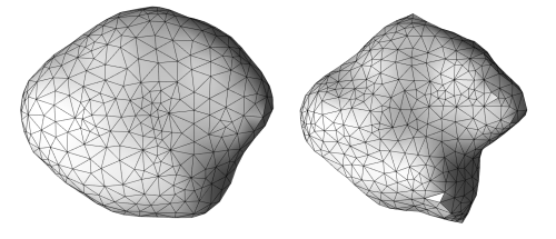
All GREs are generated as volume meshes, even though the YORP-RAT methodology only requires the definition of the body surface. The usage of volume mesh guarantees more accurate compatibility of the methodology with future addition of a model of thermal emission.
3. YORP RADIATIVE TORQUES OF A DARK BODY
The Lommel-Seeliger law describes scattering from bodies with a low albedo, such as many asteroids and the Moon. The Lommel-Seeliger (LS) reflectance is defined as
 (1)
(1)
where ῶ is the single-scattering albedo, P(α) is the single-scattering phase function, μ0= cos i of incident angle i, μ = cosϵ of emitted angle ϵ (both measured against the surface normal of an area element) and α is the common phase angle. The scattering of incient radiation produces radiation pressure, which for an irregular body is distributed unevenly across the surface, producing a net torque about the center of mass of the body. The total torque may be written as
 (2)
(2)
where the radiation pressure per area element is given by
 (3)
(3)
Above, Ω+ is the hemisphere on top of an area element, 1V is an indicator function of whether or not the area element is visible and illuminated, c is the speed of light and F0 is the radiant flux density on the body surface.
When () is inserted into (), the Ω-integral may be computed analytically for the Lommel-Seeliger case. The integral corresponds to the so-called hemispherical albedo, and can be written as
 (4)
(4)
Altogether, it is most illuminating to work with a normalized total torque
 (5)
(5)
To analyse the YORP-RATs, the total torque must be solved as a function of the body orientation. We work in coordinates, where illumination is along the x-axis, and the observer is in the (x, z)-plane. In Figure , the orientation of the body axis is given by angles θ and ϕ, around which rotations fix the body orientation.

4. CONCLUSIONS
The final poster presentation will include an interactive script based on the theory above and extensive analysis of the properties of YORP-RATs.
REFERENCES
Hoang & Lazarian, 2008, MNRAS, 388, 117
Lazarian & Hoang, 2007, MNRAS, 378, 910
Lumme & Bowell, 1981, AJ, 86, 1694
Muinonen & Pieniluoma, 2011, JQSRT, 112, 1747
Rubincam, 2000, Icarus, 148, 2
van der Walt, Colbert, & Varoquaux. 2011, CSE, 13, 22
How to cite: Herranen, J.: YORP scattering torques on Gaussian random ellipsoids, Europlanet Science Congress 2020, online, 21 Sep–9 Oct 2020, EPSC2020-792, https://doi.org/10.5194/epsc2020-792, 2020.
Please decide on your access
Please use the buttons below to download the presentation materials or to visit the external website where the presentation is linked. Regarding the external link, please note that Copernicus Meetings cannot accept any liability for the content and the website you will visit.
Forward to presentation link
You are going to open an external link to the presentation as indicated by the authors. Copernicus Meetings cannot accept any liability for the content and the website you will visit.
We are sorry, but presentations are only available for users who registered for the conference. Thank you.