Poster presentations and abstracts
This session welcomes all presentations on Mars' interior and surface processes. The aim of this session is to bring together disciplines as various as geology, geomorphology, geophysics, mineralogy, glaciology, and chemistry. We welcome presentations on either present or past Mars processes, either pure Mars science or comparative planetology, either observations or modeling or laboratory experiments (or any combination of those). New results on Mars science obtained from recent in situ and orbital measurements are particularly encouraged, as well as studies related to upcoming missions (ExoMars, Mars 2020, Mars Sample Return).
Session assets
Introduction: The OMEGA experiment onboard the ESA Mars Express orbiter [1] had observed the Martian surface in the 0.38 – 5.1 µm spectral range from 2004 to 2010. Additional observations with a limited spectral coverage are still ongoing. The dataset contains thousands of hyperspectral cubes covering most of the Martian surface with a typical spatial sampling of 1 km. Repeated observations of the same region have been frequently obtained over the mission, in particular in the high latitudes where time sampling can be about 10° of Ls over most of the year [2]. This spectral range covers water-related spectral signatures of the surface, the most prominent being located at 1.9 and 3 µm [3-6]. Previous studies of the water content derived from the 3 µm band have shown an overall increase of water hydration in the polar regions, with a modeled weight% increased by a factor greater than two in the northern polar latitudes, which presents the highest hydration state levels [5, 6].
The origin of this latitudinal trend is not yet fully understood, although two main hypotheses have been previously suggested and discussed: adsorption of water molecules at the surface (e.g. [5]) and chemical alteration from water molecules deeply bound into minerals or amorphous materials at the surface [6, 7]. We e.g. know that northern polar regions harbor salts, either in the form of large localized deposits of sulfates [8] or at low level in soils [9], as revealed in particular by the in-situ detection of low amount of perchlorates and carbonates from Phoenix [10, 11] not yet identified with orbital observations [12].
In addition, the presence of a significant amount of sub-pixels water ice patches in the polar regions may also result in an average increase of the 3 µm feature when observed at OMEGA resolution. Indeed, recent studies have shown that erosion can create scarps that expose the perennial near-surface water ice contained in the permafrost at latitudes about 55°N [13]. Permafrost depth decreases to a few centimeters at high latitudes while exposed ice stability increases [14], so such subpixels outcrops may be more frequent and could participate to the apparent increase of the 3 µm band depth with latitude.
Results: We have conducted a study of the joint variations of the 1.9 and 3 µm bands in the northern polar regions. Figure 1 shows the latitudinal variations of near-IR “albedo” (reflectance factor at 2.5 µm), 1.9 and 3 µm band depths from an OMEGA orbit during the northern summer. To minimize the impact of the well-established dependence of the 3 µm feature on albedo [3, 5, 15], we first focus on a limited albedo range ≥ 0.3. In agreement with previous studies [3,5,6], we observe that the 3 µm band depth continuously increases from 45% to 55% between 50°N and 70°N. We also observe a similar trend for the 1.9 µm band depth that goes from 2% to 4%. Thus, there seems to be a correlation between the latitude dependence of these two bands at global scale. This co-evolution is notably expected in the case of adsorbed water [4]. It may also results from an increase in the amount of trace minerals in soils, like hydrated sulfates that contains a 1.9 µm band, that may be also widespread at polar latitudes [9]. Investigations are ongoing to favor one of these two possible explanations.

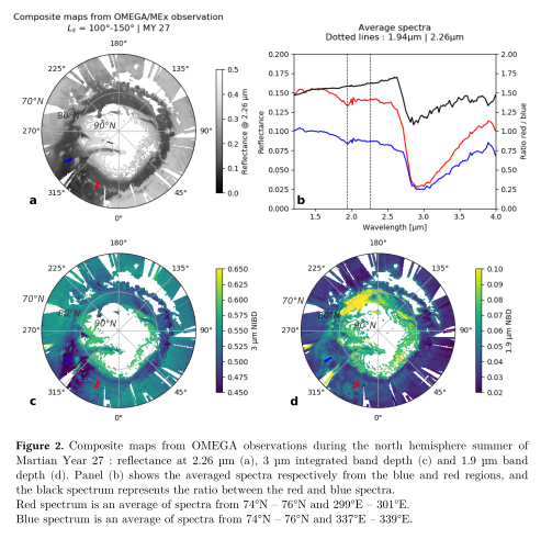
On the other hand, we can also observe some regional differences of the co-evolution of these two bands, for areas at the same latitude and that presents similar albedo values like in the northern latitudes of Acidalia Planita. Indeed, we can see on figure 2 that at ~ 75°N, there is a darker region between 290°E and 350°E (a). This region is associated with high and stable values of the 1.9 µm band (d). On the other hand, the 3 µm band changes significantly with longitude over the region (c), from 46% at 300°E to 52% at 340°E. The blue and red spectra on figure 2(b) show averaged spectra from two spots in this darker region, and the black spectrum is the ratio between the red (high 3 µm) and the blue (low 3 µm) spectra. We observe with this ratio that there is actually no 1.9 µm band variations between this two spots, whereas variations are notable for the 3 µm band.
Conclusion: These first investigations have highlighted the multiplicity of evolution behavior of the 1.9 µm and 3 µm band for different scales. Further work will be dedicated to deeper investigations of the co-evolution of the two bands at a regional scale, and their possible link with other spectral signatures. Our objective is to extend the amount of observational constraints related to the polar increase of the surface hydration observed in the 3 µm spectral range, to bring new constraints about the plausibility of the main two considered hypotheses: adsorbed water versus chemical alteration.
Acknowledgments: The OMEGA/MEx data are freely available on the ESA PSA at https://archives.esac.esa.int/psa/#!Table%20View/OMEGA=instrument .
References: [1] Bibring et al. (2004) ESA Publication Division, 1240, 37-49. [2] Langevin et al. (2007) JGR, 112, E08S12. [3] Milliken and Mustards (2005) JGR, 110, E12001. [4] Pommerol et al. (2009) Icarus, 204, 114-136. [5] Jouglet et al. (2007) JGR, 112, E08S06. [6] Audourd et al. (2014) JGR Planets, 119, 1969-1989. [7] Beck et al. (2015) EPSL, 427, 104-111. [8] Langevin et al. (2005) Science, 307, 1584-1586. [9] Massé et al. (2012) EPSL, 317-318, 44-55. [10] Boynton et al. (2009) Science, 325, 61-64. [11] Hecht et al. (2009) Science, 325, 64-67. [12] Poulet et al. (2010) Icarus, 205, 712-715. [13] Dundas et al. (2018) Science, 359, 199-201. [14] Smith et al. (2009) Science, 325, 58-61. [15] Pommerol and Schmitt (2008), JGR, 113, E10009.
How to cite: Stcherbinine, A., Vincendon, M., and Montmessin, F.: Martian surface aqueous alteration from the study of the combined evolution of the 1.9 and 3 microns band with OMEGA, Europlanet Science Congress 2020, online, 21 Sep–9 Oct 2020, EPSC2020-738, https://doi.org/10.5194/epsc2020-738, 2020.
Introduction: Oxia Planum (OP) will be the landing site of ‘Rosalind Franklin’ (RF), the ExoMars 2020 rover (Figure 1). With the primary goal of searching for signs of past and present life on Mars, the ExoMars rover will investigate the geochemical environment in the shallow subsurface over a nominal mission of 218 martian days (sols) [1]. Two science criteria for landing site selection were ancient terrains, representing the time at which Mars was at a peak of habitability, and a recent surface exposure age, minimizing cosmic ray bombardment and associated damage to organic biomarkers - key targets for Rosalind Franklin’s analytical instruments [1]. Oxia Planum contains ancient clay-bearing terrains and has undergone significant burial and erosion, with some terrains having been recently exposed, so it is an ideal site.
The landing site contains impact craters, the distribution, and degradation of which can tell us where and when burial and erosion processes have occurred. Here we: (1) Present an impact crater degradation classification scheme and database (Figure 2) [2]; (2) Report the likelihood of degradation morphologies occurring together; (3) Use the database to explore the timing of resurfacing events in OP, and; (4) Consider the implications for the geological evolution of the OP site and the wider Chryse/Arabia margin.
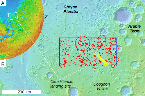
Figure 1: The location of Oxia Planum study area (blue square), the Exo-Mars landing site (yellow ellipses), impact craters (red).
Data: We developed a crater degradation classification scheme based on morphologies observable in 5–6 m/pixel CTX [3] and digitized on Murray Lab global CTX mosaic tiles; E028N16 and E024N16 [4]. We also used THEMIS [4] data overlain by the MOLA topography data to identify subtle relief patterns indicating buried “ghost craters”.
Methodology: All impact craters >500 m in diameter in the OP region (Figure 1) were recorded and classified. Classification is based on the deviation from a pristine morphology by post-impact burial and degradation processes in four aspects of their morphology: (1) Stratigraphic relationship, (2) cross-sectional shape, (3) crater rim morphology, and (4) ejecta morphology. From the database, we performed a quantitative analysis to assess the probability of different degradation morphologies occurring together using the open-source Anaconda Software Python/R data science packages. We used to use the Impact Crater Size Frequency Distributions (CSFD) of the different populations of craters, based on their ‘stratigraphic relationship’ criterion, to explore the timing of regional burial and erosion process events.
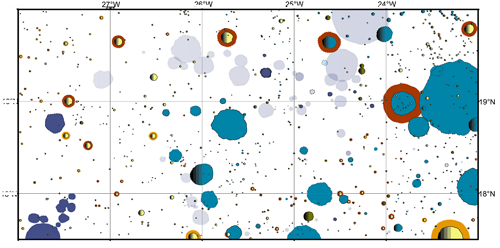

Figure 2: The distribution of impact craters in the Oxia Planum study area and the symbolization illustrating the 4 classes of degradation morphology.
Results: The classification shows that there is a generally consistent relationship between different morphological aspects of impact crater morphology as craters degrade, forming a general trend. The distribution of different degradation morphologies (Figure 2) highlights where different burial and erosion processes have occurred history of Oxia Planum.
To understand when these events happened we evaluated the CSFD for populations of craters with different degradation states (Figure 3). Craters that have not been infilled tell us the time since there has been substantial sedimentation and craters that retain sharp rims and do not have eroded ejecta tell use the time since there has been substantial regional erosion (Figure 4a). By considering buried craters, and those with removed rims embayed by younger terrain, we determine a minimum age of the basement (Figure 4b).

Figure 3: Cross-sections illustrating the time sequence of different classes within the ‘stratigraphy’ classification of impact craters [2].
Discussion & Conclusions: The model ages and distribution of impact craters with different states of burial and erosion suggest that different processes have occurred in OP at different times. Close inspection of the geological setting of these crater populations shows that:
(i) The ~4.0 Ga regional basement contains light-toned, layered, clay-bearing terrains. The light-toned surfaces host the most heavily degraded craters, and in the areas where craters have been buried, this is likely to be the underlying material in which the now buried craters formed. Furthermore, these impact craters are systematically found at lower elevations. Given the context of the study area, at the termination of a substantial ancient channel system (Coogoon Valles) into a very large basin (Chryse Planitia), we hypothesize that fluvial, lacustrine or possibly thalassic processes eroded and infilled these craters.
(ii) Although the depositional processes had stopped by ~3.5 Ga there was still widespread erosion, degradation, modifying the rims, and removing ejecta from craters. The bowl-shaped (not infilled) floors of those craters which still retain degraded ejecta suggest that all fluvial, or other heterogeneous depositional, activity in the region had ceased by this time.
(iii) All impact craters with sharp rims and preserved ejecta are younger than ~3.0 Ga. This suggests that since this time there have been substantially lower rates of erosion compared to the preceding ~0.5 Ga. This is consistent with global trends and implies that the removal of any regional overlying strata, such as might be represented by remnant rounded, buttes [6,7 ], occurred before this time.


Figure 4: The CSFD for impact craters which (a) overly the clay-bearing terrains and (b) underlay, or are found within, these clay-bearing units
Acknowledgment: The Open University’s ‘Space Strategic Research Area’ for funding A. Roberts’
References: [1] Vago, J. L. et., al. 2017 Astrobiology 17, 471–510. [2] Roberts et al., 2020 in prep, [3] Malin et al., (2006) [4] Dickson et al., 2018; (http://murray-lab.caltech.edu/CTX/index.html [5] Christensen et al., (2004) Space Science Reviews, 110,1 [6] Quantin-Nataf et al., 2020 in press at Astrobiology. [7] McNeil et al., 2020; This conference
How to cite: Fawdon, P., Roberts, A., and Mirino, M.: Impact Crater Degradation and the Timing of Resurfacing events in Oxia Planum., Europlanet Science Congress 2020, online, 21 Sep–9 Oct 2020, EPSC2020-55, https://doi.org/10.5194/epsc2020-55, 2020.
How to cite: Kereszturi, A., Égerházi, B., and Kondacs, F.: Differently aged intra-crater sediments next to each other on Mars, Europlanet Science Congress 2020, online, 21 Sep–9 Oct 2020, EPSC2020-93, https://doi.org/10.5194/epsc2020-93, 2020.
Introduction
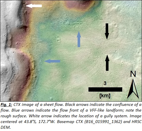
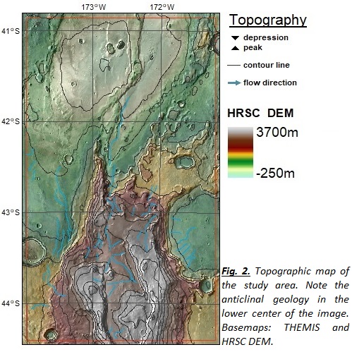
During an extensive grid-mapping campaign in the southern highlands of Mars [1], we detected sheet flow deposits on top of a mountain range in Terra Sirenum (located at 44°S, 188°E; Fig. 1,2). Although such formations have been described before near outflow channels and fissures [2,3], they were never observed on top of mountains. The related mountain rises up to 3,000 m above the surrounding plains, and appears to be formed by tectonic activities [4,5] during the Noachian [4]. It is also characterized by the highest internal heat flux values on Mars [6] and strong remnant magnetic fields [7,8]. Its general topography has similarities with a geological anticline, whose crest has been eroded, revealing an older outcrop (Fig. 2).
The high plains of the mountain consist of multiple flat valleys, whose floors are covered by an even deposit with distinct flow margins. Their surface is often characterised by lineations following the direction of the flow. They usually commence near the base of steep scarp crests. Their lengths may exceed 100 km, and their origin often coincides with viscous-flow features (VFF) [9] and gullies [10,11,12].
Methods & Results
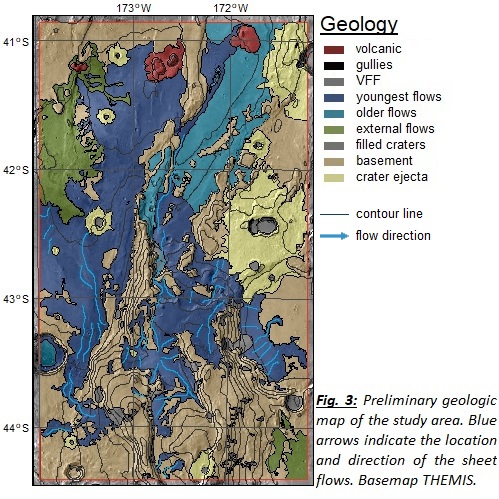
For analysing the sheet flow deposits we mapped their distribution (Fig. 3) based on CTX imagery [12], measured their thickness using MOLA single shot profiles [13], and determined their age by crater counts [14,15]. Based on these results we were able to reconstruct the stratigraphy of these flows and their relation to VFF and gullies.
Most sheet flows start at the base of steep scarp crests, following the topographic gradient down to the adjacent basins surrounding the mountain. Near these scarp crests, the flows are often covered by other deposits, resembling to VFF/glacier-like flows [9]. VFF are assumed to consist of water ice and solid particles [9]. In the study area, VFF are located in wide alcoves, steepening the adjacent crest. Their upper reaches are partially eroded or covered by gully deposits, which are assumed to be formed by water even today [11,12].
On their way down the sheet flows converge into small channels (Fig. 1) and diverge into small basins afterwards, indicating a certain viscosity of the flow material. All flows originating from the mountain emanate into two separate basins to the north where they terminate. Each of these basins contains a small volcanic edifice surrounded by lava layers [16].
The thickness values of the sheet flows vary from 5.6 to 31.7 m (based on 9 measurements), while the VFF range from 39.6 to 89.1 m (7 measurements). We also measured the thickness of volcanic flows found in the basins, having a depth of 85.3 to 103.8 m (3 measurements).
The mountain itself is lacking clear volcanic morphologies, and the relation of the flows to VFF and gullies, suggests that the sheet flows are not of volcanic origin. This assumption is supported by the age determination; while the volcanic flows are the oldest flows in the entire study area (~1.2 Ga), the sheet flows (~100 – 190 Ma) and VFF (~37 Ma) are much younger.
Discussion
Synthesizing the results, we suggest the following scenario: The mountain formed during the Noachian by tectonic processes. The small volcanoes in the basins north of it formed during the mid-Amazonian. During the latest Amazonian the sheet flows began to form (as slowly moving mud flows of high viscosity). However, we cannot yet determine the origin of the volatiles bound within the flows; they either originate from volatile-rich subsurface deposits or from atmospheric deposition in form the latitude-dependent mantle LDM, consisting of ice and dust [17]. In both cases, we suggest that the high internal heat flux [6] has triggered the melting and mobilisation of the volatiles. A preliminary screening on other mountain ranges with much lower heat flux values did not reveal further findings of such deposits. Hence, the internal heat flux can be considered a realistic scenario unleashing the volatiles.
After the sheet flows formed, they were covered by the stratigraphically more recent VFF. However, VFF show a rough morphology in contrast to the smooth sheet flows, and they are also much shorter (up to a few kilometres in length). This morphologic difference could be explained by a lower availability of volatiles, after much of the volatiles were already removed when the older sheet flows formed. The different volatile/solids-ratio of the VFF may have resulted in an even higher viscosity, and hence, different morphology. In this scenario, the volatiles have a subsurface origin rather than an atmospherical.
We also cannot exclude that the volatiles that formed both landforms (sheet flows and VFF) have each a different origin; it might be that the sheet flows originate from subsurface volatiles while the VFF originate from mobilised atmospheric volatiles (LDM).
However, it remains unknown why the sheet flows commenced during the late Amazonian and not before. But if the scenario of a warm subsurface and the presence of water is correct, the mountain could be an important location for the search of astrobiological signatures.
References
[1] Voelker et al. (2020), Icarus 346, 113806. [2] Burr and Parker (2006), GRL 33, L22201. [3] Voelker et al. (2018), Icarus 307, 1–16. [4] Tanaka et al. (2014), Geol. Map of Mars, US Geol. Survey Sci. Inv. Map 3292. [5] Karasözen et al. (2016), JGR Planets 121, 916–943. [6] Hahn et al. (2011), GRL 38 (L14203). [7] Connerney et al. (2005), Proc. Natl. Acad. Sci. USA 102 (42), 14,970-14,975. [8] Langlais et al. (2019), JGR Planets 124, 1542–1569. [9] Milliken et al. (2003), JGR 108 (E6), 5057. [10] Levy et al. (2009), Icarus 201, 113–126. [11] Dundas et al. (2010), GRL 37 (7), L07202. [12] Harrison et al. (2015), Icarus 252, 236–254. [13] Malin et al. (2007), JGR 112, E05S04; [14] Smith et al. (2001), JGR 106 (E10), 23,689–23,722. [15] Kneissl et al. (2011), Icarus 250, 384-394. [16] Michael et al. (2012), Icarus 218, 169–177. [16] Brož et al. (2015), EPSL 415, 200-212. [17] Kreslavsky and Head (2002), GRL 29 (15), 14-1–14-4.
How to cite: Voelker, M., Cardesín-Moinelo, A., and Martin, P.: The Melting Mountains of Mars? - Mud Flows in a Montane Environment, Terra Sirenum, Europlanet Science Congress 2020, online, 21 Sep–9 Oct 2020, EPSC2020-192, https://doi.org/10.5194/epsc2020-192, 2020.
One of the key elements in our search for extraterrestrial life is the availability of liquid water. Mars has been our primary target for finding life in the last decades, and the search for ancient life signs, possibly ideal terrains is still popular. In the history of the Red Planet there were presumably wetter periods [McKay et al., 1991], however on the surface of modern Mars there is little chance for the prolonged existence of larger water bodies. Theoretical models show a chance for ephemeral appearances [e.g. Brass, 1980, Kereszturi et al., 2009, Knauth and Burt, 2002, McEwen et al., 2014], while computational model results imply a microscopic scale (especially brines) emergence [e.g. Kossacki, 2008, Martínez and Renno, 2013, Möhlmann, 2004]. In this abstract we show the first results of our new research estimating the likelihood for surface perchlorate deliquescence on Mars.
We simulated the surface temperature, atmospheric pressure and water vapor volume mixing ratio for Mars year 29 using the LMDZ GCM detailed in Hourdin et al. (2006), which is the second generation of the climate model developed in the LMD described in the works of Sadourny et al. (1984) and Forget et al. (1999). From the output of the model we calculated the relative humidity with respect to ice and with respect to liquid detailed in Pál et al. (2020). There is a chance for deliquescence if both the temperature and the relative humidity with respect to liquid are above the calcium-perchlorate (Ca(ClO4)2) salt-specific threshold [Toner et al., 2014]. According to the research of Rivera-Valentín et al. (2018) if the relative humidity with respect to ice greatly exceeds 1, nucleation is favored rather than brine formation. Using this method we estimated the possibility of deliquescence on a binary scale, where 0 means no chance and 1 means definite chance.
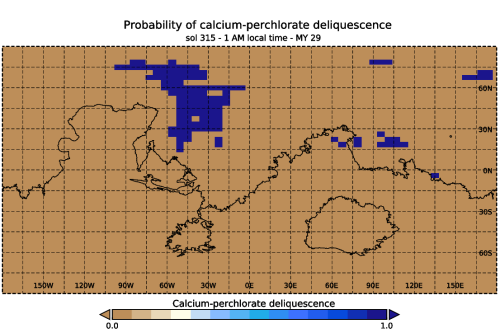
The possibility of deliquescence on a binary scale at 1 AM local time on sol 315 (the middle of northern summer). There is a larger area around Acidalia Planitia, where we see definite chance between the late northern spring and early northern autumn. We see a less defined, but persistent probability in the southern region of Utopia Planitia. This is a snapshot from the annual studies. 
Averaged probabilites of calcium-perchlorate deliquescence through the Mars year 29 at 1 AM local time. There is a rather consistent possibility between Ls 120 - 315 in the northern hemisphere, as well a during the southern summer (Ls 450 - 550) in the southern upper latitudes.
This work was supported by the EXODRILTECH project of ESA and the Excellence of Strategic R&D centers (GINOP-2.3.2-15-2016-00003) project of NKFIH, Hungary and the related H2020 fund, the COOP-NN-116927 project of NKFIH and the TD1308 Origins and evolution of life on Earth and in the Universe COST actions number 39045 and 39078.
How to cite: Pál, B. and Kereszturi, Á.: Binary maps detailing the possibility of liquid water through deliquescence on Mars, Europlanet Science Congress 2020, online, 21 Sep–9 Oct 2020, EPSC2020-225, https://doi.org/10.5194/epsc2020-225, 2020.
The erosion on Mars is poorly understood, especially the fluvial erosion, which modified obviously the surface of the Red Planet. There are several erosion models for the terrestrial environment. These models are without climbing completeness: USLE, USPED and SIMWE [1]. All of the listed models use physical variables, but most physical variables are available on SIMWE (SImulated Water Erosion) model. These are: elevation model, first order derivative of the slope (E-W and N-S direction), runoff infiltration rate, Manning’s value, rain event duration (min) and unique value (mm/hr), detachment coefficient, transport coefficient, critical shear stress. These variables are divided in two different GRASS GIS scripts: r.sim.water [2] and r.sim.sediment [3].
A former simulation used the SIMWE model on a Martian valley system, which is near to Tinto Vallis, in this case it is called Tinto B (2°55’ S, 111°53’ E). The first type of SIMWE model used the erodibility parameter (K-factor, based on the TES dataset), 15 mm/hr rain event, which held 5 minutes and used the default given parameter for the detachment (Dc) and the transport (Tc) coefficiente and critical shear stress. With these settings the SIMWE model gives a detailed map, which shows the small drainages, which are non- or barely visible on the CTX images. The second version of the model modified parameters, which come from the THEMIS thermal-inertia dataset. The K-factor sand related variable was modified with the normalised value of the thermal-inertia (local maximum of thermal-interia = 1). The variables for the detachment and transport coefficients were calculated also from the thermal-inertia values, and are equivalent with the sediment diameter sizes [4]. These converted sizes re related to the Shields parameter and critical bed shear stress [5]. From these variables the the detachment and the transport coefficient can be determined with the following equations: Tc=A/(𝛶*𝜌w1/2*gM) [6]; Dc=Kfac*(𝜏-𝜏c) [7], where Tc - transport coefficient, Dc - detachment coefficient, 𝛶 - Shields parameter, 𝜌w - density of water, gM - Martian gravity, Kfac - erodibility factor, 𝜏 - shear stress, 𝜏c - critical shear stress, A - variable from (cikk). The produced new estimated erosion-deposition map gives more detailed results, than the results in phase 1 [8], especially on the accumulation region of the small drainages. These more detailed results can give more information about the possible points of interest for further missions.
The model is still under improvement to adapt to the Martian environment. In this second phase the detachment and the transport coefficient have been determined, using the dataset of THEMIS thermal-inertia. In this case, all of the applied elevation datasets for the SIMWE model have to be reducatet to 100 m/px.
Acknowledgement: This work was supported by the GINOP-2.3.2-15-2016-00003 fund of NKFIH
References:
[2] Neteler, M. and Mitasova, H., 2008, Open Source GIS: A GRASS GIS Approach. Third Edition. The International Series in Engineering and Computer Science: Volume 773. Springer New York Inc, p. 406.
[3] Mitasova, H., Thaxton, C., Hofierka, J., McLaughlin, R., Moore, A., Mitas L., 2004, Path sampling method for modeling overland water flow, sediment transport and short term terrain evolution in Open Source GIS. In: C.T. Miller, M.W. Farthing, V.G. Gray, G.F. Pinder eds., Proceedings of the XVth International Conference on Computational Methods in Water Resources (CMWR XV), June 13-17 2004, Chapel Hill, NC, USA, Elsevier, pp. 1479-1490.
[4] Fenton, Lori. (2003). Aeolian processes on Mars: atmospheric modeling and GIS analysis. (Phd thesis, CALIFORNIA INSTITUTE OF TECHNOLOGY )
[5] Berenbrock, Charles; Tranmer, W., Andrew; Simulation of Flow, Sediment Transport, and Sediment Mobility of the Lower Coeur d’Alene River, Idaho, 2008, USGS Scientific Investigation Report, pp 43.
[6] Lamb, M. P., Dietrich, W. E., and Venditti, J. G. ( 2008), Is the critical Shields stress for incipient sediment motion dependent on channel‐bed slope? J. Geophys. Res., 113, F02008, doi:10.1029/2007JF000831.
[7] M.S. Kuznetsov, V.M. Gendugov, M.S. Khalilov, A.A. Ivanuta,; An equation of soil detachment by flow; 1998; Soil and Tillage Research,; vol 46; issues 1-2; pp 97-102
[8]Vilmos, Steinmann; László, Mari; Ákos, Kereszturi; 2020; Testing the SIMWE (SIMulate Water Erosion) model on a Martian valley system; EGU 2020 abstract; Wien
How to cite: Steinmann, V. and Kereszturi, Á.: Results of a modified physical based erosion model (SIMWE) on a Martian environment, Europlanet Science Congress 2020, online, 21 Sep–9 Oct 2020, EPSC2020-227, https://doi.org/10.5194/epsc2020-227, 2020.
Abstract
Laboratory measurements were performed on different mixtures made with clays and organic compounds with the aim of characterizing the detection capabilities of biosignatures by the Ma_MISS (Mars Multispectral Imager for Subsurface Studies) instrument.
Introduction
The main scientific objectives of the ESA mission ExoMars2022 are searching for signs of past and/or present life on Mars and characterizing the subsurface geochemical environment as a function of depth. The Rosalind Franklyn rover [1] payload consists of a suite of nine instruments that will provide information about the geological and geochemical environment of the surface and subsurface of the selected landing site (i.e. Oxia Planum) [2]. Remote sensing measurements performed by OMEGA and CRISM suggest that the exposed rocks on the surface of Oxia Planum experienced an intense aqueous alteration [3]. The widespread presence of Fe/Mg-Al-phyllosilicates and, more generally, the presence of silicates containing OH confirm the interaction between water and mother rocks, which is a prerequisite favorable to the development of life. In this framework, we performed several spectroscopic measurements of clay minerals mixed with different organic compounds, to assess Ma_MISS capability of organic’s detection in the Martian subsurface.
The Ma_MISS instrument
Ma_MISS is the Visible- and Near-Infrared miniaturized spectrometer hosted in the drill system of the ExoMars2022 rover that will characterize the mineralogy and stratigraphy of the excavated borehole wall at different depths (<2 m) [4]. Ma_MISS with a spectral range of 0.5–2.3 μm, a spectral resolution of about 20 nm in the IR, a SNR~100, and a spatial resolution of 120 μm will accomplish the following scientific objectives: (1) determine the composition of the subsurface materials; (2) map the distribution of the subsurface H2O and hydrated phases; (3) characterize important optical and physical properties of the materials (e.g., grain size); (4) produce a stratigraphic column that will provide information on the subsurface geology. Ma_MISS will operate periodically during pauses in drilling activity and will produce hyperspectral images of the drill’s borehole.
Experimental setup
The characterization of the scientific performances of the Ma_MISS instrument was made using the laboratory model (breadboard, Fig. 1 [5], [6]) at the Institute for Space Astrophysics and Planetology – INAF. The Ma_MISS breadboard includes the 5 W light source, the optical fibers, and the Optical Head with the dual task of focusing the light on the target and recollecting the scattered light. However, it does not include the flight spectrometer and is therefore coupled with a laboratory spectrometer (FieldSpec 4).
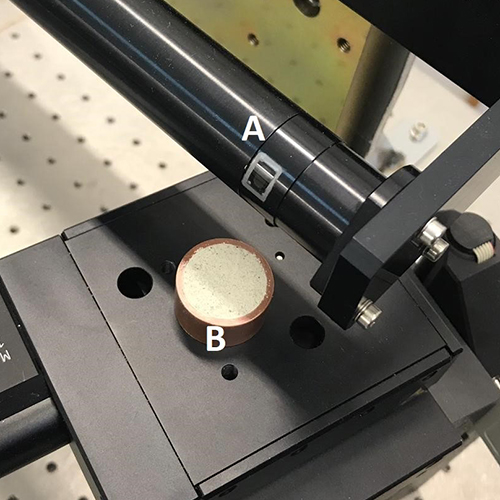
Fig. 1: Ma_MISS breadboard setup. A: Ma_MISS Optical Head; B: sample holder.
Clay/organic mixtures measurements
For these tests we prepared numerous samples mixing two clay minerals (nontronite and kaolinite) with four different organic compounds (asphaltite, glycine, benzoic acid, and polyoxymethylene). In particular, starting from the pure clay endmembers we tested two cases. In the first case, we added separately asphaltite and glycine in the following percentages: 25, 50, and 75, producing six different samples with high organics concentration. In the second case, we added separately benzoic acid and polyoxymethylene in percentages of 1, 5, and 10% preparing a set of six samples at a low concentration of organics. All mixtures with a grain size < 60 μm were measured using the Ma_MISS breadboard setup collecting reflectance spectra in the range 0.5–2.3 μm. Figure 2 shows an example of the data collected on the mixtures between kaolinite and glycine. Starting from the spectra of the pure clay (kaolinite 100%, black spectrum in Fig.2) and increasing the content of glycine by step of 25 wt.%, the band at 1.4 μm associated to the presence of the OH bond in kaolinite decreases. At the same time the band at 2.1–2.2 μm linked to the Al–OH bond in kaolinite become wider and much stronger due to the superimposition of the wider CH band of glycine at 2.1–2.25 μm.
Other mixtures with other types of organics in a concentration below the 1% are still in preparation with the aim of determining the lower detection limit of the instrument in the function of the different hosting minerals. In these tests, we used glycine and other organic compounds, as examples of organic compounds that show absorption features in the VIS-NIR range, although we do not expect to find these specific organics in the Martian subsurface.
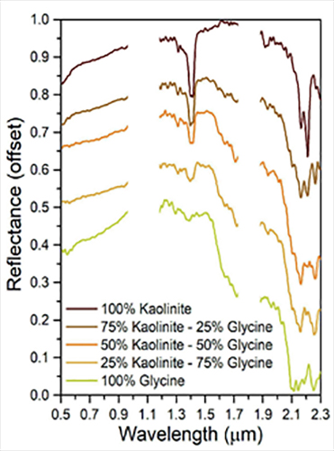
Fig. 2: Example of Ma_MISS breadboard measurements of mineral/organic mixtures (kaolinite-glycine) in variable proportion.
Conclusions
Laboratory investigations have been performed using the Ma_MISS breadboard model (coupled with a FieldSpec Pro) on mineral/organic mixtures in different proportions. Spectroscopic measurements collected on these mineral/organic mixtures are useful to characterize Ma_MISS instrument sensitivity in detecting traces of life intimately mixed with minerals that could be present in sedimentary sequences or in hydrothermal products in the Martian subsurface, which is one of the main scientific objectives of the ExoMars2022 mission. The obtained results show that the Ma_MISS instrument can give hints of the presence of organics in the Martian subsoil, as well as characterizing the mineralogy of the drilling site. Moreover, the selected minerals and organic compounds allow us to test the instrument with both dark and bright samples. The spectra obtained during these tests will allow us to build a spectral database useful for the interpretation of the scientific data.
Acknowledgments
We thank the European Space Agency (ESA) for the ExoMars Project, ROSCOSMOS and Thales Alenia Space for rover development, and Italian Space Agency (ASI) for funding and fully supporting Ma_MISS experiment.
References
[1] Vago J.L. et al. (2017): Astrobiology, 17, 6, 7. [2] Quantin C. et al (2016) #2863, 47th LPSC, Houston, TX. [3] Carter J. et al. al (2016) #2064, 47th LPSC, Houston, TX. [4] De Sanctis M.C. et al. (2017): Astrobiology, 17, 6, 7. [5] De Angelis S. et al. (2014): PSS, 101, 89-107. [6] De Angelis S. et al. (2017): PSS, 144, 1-15.
How to cite: Ferrari, M., De Angelis, S., De Sanctis, M. C., Altieri, F., Ammannito, E., Frigeri, A., Formisano, M., Mugnuolo, R., and Pirrotta, S.: Testing the Ma_MISS instrument capabilities for organics detection, Europlanet Science Congress 2020, online, 21 Sep–9 Oct 2020, EPSC2020-348, https://doi.org/10.5194/epsc2020-348, 2020.
Introduction
Alteration of mafic and ultramafic rocks on Mars surface and shallow subsurface has been postulated to have occurred throughout its history by means of different mechanisms, among which acid groundwater circulation (mainly sulfuric) is one of the most important [1,2,3,4]. This hypothesis is based on the high Fe and S concentration observed at various landing sites and strengthened by remote-sensing infrared detection of Fe/Al-bearing sulfates such as alunite, jarosite and Fe3+SO4(OH) [4,5]. These sulfates typically form as alteration of K-rich volcanic rocks and Fe-sulfides in low-pH environments. Additionally the occurrence of perchlorates could be related to the action of other acids (perchloric) [6]. The investigation in laboratory of acidic alteration of volcanic rocks is thus an essential step in order to provide constraints in the interpretation of remote-sensing and in-situ data from Mars missions of the next future (Mars-2020, ExoMars-2022). Several works recently have explored the processes of acid alteration of minerals and rocks both in the field and in laboratory by using different spectroscopic and microscopy techniques [7,8].
Methods
In our work we studied by Visible-Near Infrared reflectance and Raman spectroscopy the acid alteration of two volcanic samples, a basalt from Aeolian Islands (FCD1) and a rhyodacite from Alps (RDO). These two samples have been chosen with the aim of investigating the action of acids on both a mafic and a felsic rock. Four acids have been used for the treatment of samples, namely hydrochloric (HCl 37 vol%), nitric (HNO3 65 vol%), sulfuric (H2SO4 96 vol%) and phosphoric (H3PO4 85 vol%), in order to contemplate a diversity of acid environments. Samples were acid-treated both in the form of fine powders (d<50 μm) and slabs. For each of the two volcanic samples four aliquots of powders were produced, with the aim of allowing different durations of alteration, and kept in solution for 1 h, 24 h, 7 days and 6 months respectively. At the end of each time slot the aliquot was centrifuged at 9500 rpm for 5 minutes, the excess liquid removed, and dried at 70°C in desiccator prior of measurements. The rocks slabs were instead kept in contact with acid for a few days and subsequently dried.
VIS-NIR reflectance spectroscopy measurements were carried on with ASD FieldSpec-4 spectro-photometer coupled with a QTH lamp and optical fibers (i=30°, e=0°), in the 0.35-2.5-μm range, using LabSphere Spectralon as reference. The spectral sampling was 3-8 nm, and the spatial resolution about 6 mm.
Raman spectroscopy data were acquired with a Bruker-Senterra II spectrometer, with a 532 nm excitation laser, a power of 50 mW, 4 cm-1 spectral resolution, and about 5 mm of spatial resolution. Raman data were acquired on pre- and post-treatment slab samples.
Results
VIS-NIR. We present preliminary results of our experiments. Example of VIS-NIR spectra are shown in fig.1 for the basalt FCD1. The spectrum of pre-treated basalt (black curve, fig.1) is characterized by iron absorption features at 0.52 μm and 1 μm (faint), with a blue slope below 1.5 μm and a red slope above 1.5 μm. Although the effect due to some hydration is unavoidably present in the treatment, nevertheless the different acids produce different results. The overall spectral shape does not change much after treatment with HCl and HNO3, although new absorption features appear or increase in intensity. In the HCl-treated sample the 1-μm band is notably more marked than the pre-existing one, and new features appear at 1.44, 1.60, 1.75, 1.93, 2.15 and 2.24 μm. Although especially the ~1.4 and ~1.9-μm bands are related to hydration in the sample or to some new hydrated phase, nevertheless these new bands indicate the appearance of new mineralogical phases. For example some of these bands are reported to occur in hydrated Na-perchlorates [9]. Curiously in the HCl-treated sample the ~0.5-μm feature seems to disappear. In the H2SO4-treated sample the overall spectral slope is changed from red to blue, and only two hydration bands appear. In the HNO3-treated sample a new weak band appeared around 2.23 μm.
Raman. The Raman spectra of an alkali-feldspar phenocryst of the rhyodacite sample (RDO) collected pre- and post-treatment with HNO3 are displayed in fig.2 (black and red, respectively). The spectrum of the untreated sample is characterized by the typical Raman peaks of the alkali-feldspar. On the contrary, in the spectrum of the acid-treated sample, the appearance of the peaks at 1053 and 715 cm-1 indicate the formation of niter (NaNO3) in the same areas of the sample where the alkali-feldspar is present.


Conclusions
Visible-infrared and Raman analyses of both mafic and felsic volcanic rocks treated with different acids have shown the appearance of new absorption bands and changes in spectral shapes, indicating the formation of new mineralogical phases. While Raman data clearly indicate the presence of precise minerals, the interpretation of VIS-NIR spectra is not straightforward. Further analyses will be conducted both on the powders and slabs in order to recognize the new mineralogical phases, to discriminate between the alteration action of acid solution and water alone, and to disentangle the effects of the different acids over time.
Acknowledgements
This work is funded by ASI. We thank A.Pisello from University of Perugia for providing the rhyodacite sample.
References.
[1] Burns R.G., Journal of Geophysical Research, vol.92, n.B4, pp.E570-E574, 1987
[2] Burns R.G., 19th Lunar and Planetary Science Conference, 46-47, 1988
[3] Burns R.G. and Fisher D.S., Journal of Geophysical Research, vol.95, n.B9, pp.14,415-14,421, 1990
[4] Hurowitz J.A. and McLennan S.M., Earth and Planetary Science Letters, 260, 432, 443, 2007
[5] Ehlmann B.L. and Edwards C.S., Annu. Rev. Earth Planet. Sci., 42, 291-315, 2014
[6] Wilson E.H., Journal of Geophysical Research:Planets, 121, pp.1472-1487, 2016
[7] Gurgurewicz J. et al., Planetary and Space Science, 119, 137-154, 2015
[8] Smith R. et al., Journal of Geophysical Research:Planets, 122, pp.203-227, 2017
[9] Hanley J. et al., Journal of Geophysical Research:Planets, 119, pp.2370-2377, 2014
How to cite: De Angelis, S., Ferrari, M., De Sanctis, M. C., Altieri, F., Ammannito, E., Fonte, S., Formisano, M., Frigeri, A., and Giardino, M.: VIS-NIR and Raman analyses of acid altered volcanic rocks, Europlanet Science Congress 2020, online, 21 Sep–9 Oct 2020, EPSC2020-529, https://doi.org/10.5194/epsc2020-529, 2020.
We are developing a machine learning system based on high-resolution images of Earth and Mars for classifying periglacial landscape features, detecting their temporal changes, and assessing their global distribution as well as their potential as indicator for climate conditions and changes.
Earth periglacial landscape phenomena such as ice wedge polygons are closely linked to repeated freeze-thaw cycles, and the presence of water and ice in the subsurface. Ice wedge polygons, which are widespread in Arctic lowlands, constitute an important indicator for ground ice content. Ground ice makes permafrost vulnerable to thaw and subsidence, thus leading to massive changes in topography, hydrology, and biogeochemical processes [1]. Moreover, variations in permafrost extent due to climate warming in Earth’s polar regions cause changes in the aforementioned periglacial features.
On Mars, similar young landforms such as ice-wedge polygons and debris flows are found [2]. Large volumes of excess ice are known to exist in the shallow subsurface of mid-latitude regions [3]. A major debate focusses on whether similar freeze-thaw cycles thawed this excess ice in the geologically recent past. If true, this would be conflicting with the current Martian environment, which ostensibly prevents the generation of liquid water, and would therefore have implications for the recent hydrologic past of Mars. With liquid water also intrinsically linked to the climate evolution and the potential habitability of Mars, the investigation of the aforementioned landforms becomes essential. Moreover, the present-day surface of Mars experiences changes linked to H2O and CO2 ice, which are unlikely to be the result of aqueous processes [4, 5]. Detecting the magnitude and timing of these changes would enable the estimation of the related process rates [6, 7] and the testing of hypotheses regarding the formation mechanism.
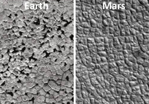
Polygons on Earth (source:[1]) and Mars (source: [8])
Quantification of periglacial features on regional- to global-scale has not been done for either of the planets so far. These features as well as their changes can be tracked with high resolution remote sensing across large regions using big data approaches of image processing, classification and feature detection. For Earth the detection and tracking of periglacial features would provide invaluable insights into periglacial and permafrost dynamics as well as in the potential for permafrost vulnerabilities to thaw in a warming world. For Mars, determining the distribution of such landforms, as well as the spatial relationship to each other and to external parameters such as topography, would provide clues for their formation and thus elucidate the role of liquid water in the recent past.
The key task is to map selected features across large regions using large high-resolution datasets, which makes automated methods for detection and classification of landforms essential. We are developing a powerful machine learning system that will identify the most appropriate image features for each landform. It will be trained on images for different cases of periglacial landforms. Ice wedge polygons are morphologically very similar on both planets, which besides the opportunity to conduct analogue studies, also provides the possibility to combine training datasets from both planets. Our system will be validated by manual identification of periglacial features on images, as well as with the existing validation datasets of both planets.
Our project is exploring the potential for a machine learning system to detect periglacial phenomena by exploiting big datasets of large regions of Earth and Mars. The resulting global-scale mapping of ice wedge polygons will provide insights regarding the permafrost vulnerabilities to changing climates on Earth, as well as about the recent role of liquid water on Mars. The former are linked to life and biogeochemical processes on Earth, while the latter to the evolution of climate and potential habitability of Mars.
Acknowledgements
This work is funded by Geo.X, the research network for geosciences in Berlin and Potsdam.
References
How to cite: Fanara, L., Hauber, E., Hänsch, R., Gwinner, K., Oberst, J., Rettelbach, T., Morgenstern, A., and Grosse, G.: Global-scale mapping of periglacial landforms on Earth and Mars, Europlanet Science Congress 2020, online, 21 Sep–9 Oct 2020, EPSC2020-583, https://doi.org/10.5194/epsc2020-583, 2020.
Abstract
We performed thermophysical simulations of Oxia Planum, the landing site of the ExoMars 2022 mission [5]. The numerical simulations concern: I) the influence of the thermal inertia on the subsurface temperature at the latitude of Oxia Planum; II) the heat released in the subsurface by the drill installed on the ExoMars rover. The numerical simulations are performed using a 3-D model using the discretization technique of the finite element method (FEM).
1. Introduction
Numerical simulations are required to characterize, from a thermophysical point of view, Oxia Planum, the landing site of the mission ExoMars 2022. A drilling system is installed on the ExoMars rover and it will be able to analyze up 2 meters in the subsurface of Mars. The spectrometer Ma_Miss (Mars Multispectral Imager for Subsurface) [1] will investigate the lateral wall of the borehole generated by the drill, providing hyperspectral images. Among the scientific objectives of Ma_Miss there are the characterization and the mapping of possible volatiles. In this regard, numerical simulations are useful to understand if the temperatures in the subsurface are such as to preserve volatiles, especially after the heating provided during the drilling operations.
2. Numerical Method
We performed our simulations by using a 3-D finite element model [2, 3], which solves the classical heat equation in a parallelepipedal domain representing a portion of Oxia Planum, the landing site of the ExoMars mission. The top of this domain is modeled with a Gaussian random surface in order to simulate the roughness of the surface. The dimensions of the domain are 1cm x 1cm x 5cm. The depth (5 cm) has been chosen since it is compatible with the likely skin depth. At the top we imposed a radiation
boundary condition, while on the other sides zero heat flux is imposed. The initial temperature is set at 200 K, which is compatible with the surface equilibrium temperature. Self-heating between the facets of our domain is taken into account. We investigate: I) the dependence of the subsurface thermal response to different thermal inertia; II) the
heat released by the drill in the subsurface of Mars. In particular, for the point II, we assume: a) the drilling is instantaneous in a well-defined “drilling temporal window”; b) thrust and rotational velocity are constant. The contribution of the drill is taken into account by applying an heat flux (depending in particular on the thrust, angular velocity and frictional heating) on the wall of the rock matrix in contact with the drill.
3. Summary and conclusions
In Fig.1 we report an example of the results we obtained by applying our numerical model. Fig.1 shows the temperature profile vs time at different depths for two cases: case

Fig.1: Temperature profile vs time at different depths. Case (A): K = 0.045 W m−1K−1; Case (B) K = 0.0045 W m−1K−1.
(A) with a thermal conductivity K=0.045 W m-1 K-1, compatible with Insight estimation [4] and case (B) with a thermal conductivity an order of magnitude smaller than the case (A). Case (A) is characterized by a thermal inertia of 270 TIU (Thermal Inertia Units) and a skin depth of 3 cm, while case (B) is characterized by a thermal inertia of 85 TIU and a skin depth less than 1 cm. Our numerical results suggest that: a) the surface temperature ranges from 180 K to 270 K if thermal inertia is high (300 TIU); b) surface temperature ranges from 140 K to 280 K if thermal inertia is low (<100 TIU); c) the self heating can increase surface temperature of about 10 K. In Fig.2 we shows the increase of the temperature due to the drilling process. In the x-axis is plotted the distance from the hole in the direction perpendicular to the drilling direction. Four cases are explored: rpm (rotation per minute) = 30 and 60 and frictional coefficient (η) = 0.5 and 0.9. The frictional coefficient computes the efficiency of the heat transfer by the drill. We observe an increase of temperature up to 300 K from the initial temperature, in case of rpm = 60 and frictional coefficient = 0.9 Future simulations with different parameters will be carried out. Moreover, a model validation with laboratory experiments is required.
Fig.2: Left panel: rpm = 30 and η= 0.5; right panel: pm = 60 and η= 0.9.
Acknowledgements
The Italian Space Agency (ASI) has founded the experiment.
References
[1] Coradini, A., et al.: MA_MISS: Mars multispectralimager for subsurface studies, Advances in Space Research, Volume 28, Issue 8, p. 1203-1208, 10.1016/S0273-1177(01)00283-6, 2001
[2] M. Formisano, M.C. [De Sanctis], S. [De Angelis], J.D. Carpenter, and E. Sefton-Nash. Prospecting the moon: Numerical simulations of temperature and sublimation rate of a cylindric sample. Planetary and Space Science, 169:8 – 14, 2019.
[3] Rinaldi, G., Formisano, M., Kappel et al., Analysis of night-side dust activity on comet 67p observed by virtis-m: a new method to constrain the thermal inertia on the surface. A&A, 630:A21, 2019.
[4] T. Spohn et al. The Heat Flow and Physical Properties Package (HP3) for the InSight Mission, Space Science Reviews volume 214, Article number: 96 (2018)
[5] Vago et al., 2017. Astrobiology, 17 6-7
How to cite: Formisano, M., De Sanctis, M. C., Federico, C., Magni, G., Altieri, F., Ammannito, E., De Angelis, S., Ferrari, M., Frigeri, A., Fonte, S., and Giardino, M.: Thermophysical modelization of the ExoMars 2022 landing site, Europlanet Science Congress 2020, online, 21 Sep–9 Oct 2020, EPSC2020-623, https://doi.org/10.5194/epsc2020-623, 2020.
Key in the interpretation and understanding of WISDOMs ground penetrating RADAR (GPR) measurements is the capability to correctly (and efficiently) simulate the instrument characteristics and the RADAR wave propagation in the Martian subsurface (the signal received by WISDOM), taking into account all relevant effects at large scale. In this contribution we present a ray tracing approach that can be applied to heterogeneous and inhomogeneous media and includes the antenna characteristics of the WISDOM instrument as well as rover structures.
The WISDOM GPR is part of the 2022 ESA-Roscosmos ExoMars “Rosalind Franklin” rover payload. It will probe the Martian surface and subface at centimetric resolution and a penetration depth of about 3m. WISDOMs primary scientific objective is the high-resolution characterization of the material distribution within the first few meters of the Martian subsurface as a contribution to the search for evidence of past life [1] and to support the drilling operations [2].
The simulation tool consists of two parts: The first part simulates the instrument at system level and generates the signal that is fed into the antenna as well as the receive-filter and discretization characteristic of the instrument (taking into account filters, RF effects and the ADC). The second part simulates the wave propagation of this signal in complex media (inhomogeneous or heterogeneous lossy media) taking into account polarization effects and the WISDOM antenna pattern [3]. This method is a hybrid between conventional raytracing (SBR), differential raytracing and physical optics. The simulation complexity can be granularly controlled and weighed against the level of approximation. It is capable of simulating electrically large domains with an acceptable accuracy yielding good predictions of the propagation properties in Martial soil while being significantly less computationally expensive than conventional full-wave solvers like FEM or the Finite-Differences in Time-Domain Method.
The results of the system-level-simulation and the propagation simulation for multiple measurement positions (along a rover track) are then combined (similar to the application of a filter) in order to generate a synthetic radargram. This radargram can be directly compared to the WISDOM measurements.
The proposed method is validated using measurements of the WISDOM instrument at analog sites and by reference simulations using the FDTD Method [4]. We present synthetic radargrams as simulation results for several sounding scenarios including the WISDOM antenna characteristics, an inhomogeneous subsurface and lossy materials.
The proposed approximation method yields accurate estimates of WISDOM soundings for a complex subsurface while being significantly faster than conventional (full wave) methods. The synthetic radargrams can easily be compared to actual measured data.
The research on WISDOM is supported by funding from the Centre National d’Etudes Spatiales (CNES) and the Deutsches Zentrum für Luft- und Raumfahrt (DLR).
[1] V. Ciarletti, C. Corbel, D. Plettemeier, P. Cais, S. M. Clifford, S.-E. Hamran, "WISDOM GPR Designed for Shallow and High-Resolution Sounding of the Martian Subsurface", Proceedings of the IEEE, Vol. 99, Issue 5, pp. 824-836, May 2011.
[2] V. Ciarletti, S. Clifford, D. Plettemeier and the WISDOM Team, "The WISDOM Radar: Unveiling the Sub surface Beneath the ExoMars Rover and Identifying the Best Locations for Drilling", Astrobiology, Vol. 17, No. 6-7, July 2017
[3] D. Plettemeier et al., "Full polarimetric GPR antenna system aboard the ExoMars rover," 2009 IEEE Radar Conference, Pasadena, CA, 2009, pp. 1-6, doi: 10.1109/RADAR.2009.4977120.
[4] C. Statz and D. Plettemeier, "BETSi: An electromagnetic time-domain simulation tool for antennas and heterogeneous media in ground penetration radar and biomedical applications," 2017 Computing and Electromagnetics International Workshop (CEM), Barcelona, 2017, pp. 37-38, doi: 10.1109/CEM.2017.7991875.
How to cite: Statz, C., Plettemeier, D., Lu, Y., Benedix, W.-S., Hegler, S., Ciarletti, V., Le Gall, A., Corbel, C., Oudart, N., and Hamran, S.-E.: Sounding and Signal Simulation of Complex Surface and Subsurface Structures for the WISDOM GPR, Europlanet Science Congress 2020, online, 21 Sep–9 Oct 2020, EPSC2020-663, https://doi.org/10.5194/epsc2020-663, 2020.
Introduction: We consider the surface structures and geological history of Isidis Planitia on Mars. It is a plain located inside a large impact basin of ~1500 km in diameter. Its age is ~3.8 Ga ago [1, 2]. Geologic history of Isidis Planitia (or at least some of its parts) is quite complicated and many details remain unclear. We believe that better analysis of surface structures (especially chains of cones) and large deep structures (e.g. mascon) will allow a better understanding of the processes responsible for present structures of Isidis.
Formation of basin and mascon:
One of the large Martian mascon is located under Isidis. This is an anomalously high mass concentration below the surface. Such structures were discovered during the Apollo missions on the Moon. The formation of mascon is possible only under special physical conditions. Therefore, its existence is an important source of information about past conditions and can help us determine thermal conditions in the past of the basin.
We use numerical models to this problem. Preliminary results point that the model allows to determine thermal conditions and some tectonic processes in the period when the mascon was formed.
Role of comparison: Earth, Mars and Moon:
The possibility of comparing processes on different celestial bodies is important for our research [3]. Mars is a body of intermediate mass and size between Earth and the Moon. Therefore, it can be expected that some geological processes on Mars are similar to processes on Earth (e.g. volcanism) or the Moon (e.g. mascon’s formation).
Role of distributed volcanism and chains of cones:
We are examining the system of cones on Isidis Planitia. Many of these chains have a characteristic furrow through the center, suggesting that fissure volcanism along circumferential dikes was common in the Isidis area. The cones have diameter of 300–500 m and height of ~30 m. This means slopes of 7–11° which is consistent with explosive type of volcanism. Similar cones are known from Iceland (64°03′53″N 18°13′34″). Some of Isidis Planitia cones are without a furrow. We recognize this type of volcanism on the volcanic archipelago of the Canary Islands and in particular on Lanzarote. The cones on Isidis have been divided into a few types depending on their structures. Currently, we are working on determining the duration and age of their volcanic activity, as well as the size of related magma plumbing system, which might be related to Syrtis Major.
Regions of Isidis:
Our analysis of chains of cones indicates that they can be grouped in larger systems. In this way Isidis Planitia has been divided into several characteristic regions. These separated regions have characteristic pattern of cones or cone chains.
We present here two examples. They represent concentrically arranged chains of cones. Fig. 1 a, b. represent cones with a characteristic furrow passing through the center. In contrast, Fig. 2 a, b, show cones arranged concentrically around the crater, from which the outflows can be seen.. It is possible that these forms represent different origin, explosive (Fig. 1), and effusive (Fig. 2).

Figure 1a
CTX mosaic with characteristic concentric arranged cones with a characteristic furrow. Black arrows indicate the direction of the arches' propagation. White rectangle is 20 km long. Center of image: 14o51’04.22”N; 83o57’15.12”E
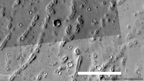
Figure 1b
Enlargement of the concentric cone area Fig. 1a. White rectangle – 4 km

Figure 2a
CTX mosaic with cones arranged concentrically around the crater. Characteristic outflows from cones are visible. Black arrows indicate the direction of the arches' propagation. White rectangle - 30 km. Center of image: 15o04’06.95”N; 81o16’14.87”E.

Figure 2b
Enlargement of the concentric cone area Fig. 2a. White rectangle - 4 km
References
[1] Ivanov, M.A., et al. 2012, Icarus. https://doi.org/10.1016/j.icarus.2011.11.029
[2] Rickman, H., et al. Planetary and Space Science, 166, 70–89, 2019.
[3] Czechowski, L., et al. 2020. LPSC 2020 in The Woodlands, Tx.
How to cite: Czechowski, L., Zalewska, N., and Ciazela, J.: Isidis Planitia: its regional and local characteristics, Europlanet Science Congress 2020, online, 21 Sep–9 Oct 2020, EPSC2020-795, https://doi.org/10.5194/epsc2020-795, 2020.
The presence of a liquid deposit of water below the South Polar Layered Deposits (SPLD) Region has been reported based on analysis of MARSIS radar data in the Planum Australe area (Orosei et al., 2018). These radar data show bright subsurface reflections that have been interpreted to be due to liquid water buried at a depth of 1.5 km (Orosei et al., 2018). The presence of such water would have important implications for the present-day thermal state of the region. Previous work based on the flexure of the lithosphere yielded a present surface heat flow of about 20–30 mW m-2 (Ruiz et al., 2010; Parro et al., 2017) at the south polar cap. Global thermal evolution models that included variations in crustal thickness and heat production estimated a global surface heat flow of 23.2–27.3 mW m-2 (Plesa et al. 2018). These estimations are difficult to reconcile with the high heat flows, in excess of 72 mW m-2 (Sori and Bramson, 2019), that are required to explain the existence of liquid water at 1.5 km deep. In this work, we aim to re-analyze the thermal state of the region and the thermal properties that are required to stabilize liquid water under the SPLD.
In order to study the thermal conditions that are compatible with the liquid water deposit, we first recalculated the depth of the bright radar reflections using a temperature-dependent relative permittivity for the water ice (Fujita et al., 2000). The depth to the putative liquid water is important, as deeper depths require lower heat fluxes to reach the melting temperature, and vice versa. We obtained a new depth to the bright reflector of 1.7 km, assuming a surface temperature of 160 K and a melting temperature of 200 K, which is appropriate if calcium perchlorate is present in the area.
Then, we calculated surface heat flows and subsurface temperatures by solving the stationary heat conduction equation. We assume that the composition of the SPLD region is a mixture of 85% of water ice and 15% of dust with a density of 1220 kg m-3 (Zuber at al., 2007). We use an ice thermal conductivity that is dependent on temperature following:

where T is the temperature in Kelvins (Fukusako, 1990). For the dust component, we assume a thermal conductivity of 2 W m-1 K-1, and calculate the thermal conductivity of the dust-ice mixture as a geometric mean (Beardsmore and Cull, 2001). We also include a superficial layer of CO2 with a thickness of 1 m, a density of 1600 kg m-3, and a thermal conductivity of 0.02 W m-1 K-1. We find that a surface heat flow of 61 mW m-2 is needed to obtain melting at 1.7 km depth. This result is still higher than the values previously estimated from lithosphere flexure in the region, but somewhat lower than that reported by Sori and Branson (2019). Additionally, fractures or voids near the surface of the SPLD at this site could reduce the thermal conductivity of the region and lower the required heat flow even further. In order to account for this possibility, we calculated surface heat flows for additional models which include an intermediate layer of lower thermal conductivity placed between the CO2 and the more conductive dust-ice mixture. Models with an intermediate insulating layer 15 m thick and with thermal conductivities between 0.05 and 0.1 W m K-1 yield surface heat flows of 41 and 50 mW m-2, respectively, to stabilize liquid water at 1.7 km depth. Further work will realize a more complete assessment of this location and of the regional heat flow context.
References
- Beardsmore, G.R. et al., (2001). Crustal Heat Flow: A Guide to Measurement and Modelling. Cambridge University Press, Cambridge, 324 pp.
- Fujita, S. et al., (2000). A summary of the complex dielectric permittivity of ice in the megahertz range and its applications for radar sounding of polar ice sheet. Physics of Ice Core Records: 185-212
- Fukusako, S., (1990). Thermophysical properties of ice, snow and sea ice. Int.J. Thermophys.11, 353–372.
- Martin-Torres F.J. et al., (2015), Transient liquid water and water activity at Gale Crater on Mars, NatGeosci8:357–361.
- Orosei R. et al., (2018). Radar evidence of subglacial liquid water on Mars, Science 1126/science.aar7268.
- ParroM. et al., (2017). Present-day heat flow model of Mars, Sci. Rep. 7, 45629; doi: 10.1038/srep45629.
- Plesa, A. C. et al., (2018). The thermal state and interior structure of Mars. Geophysical Research Letters, 45(22), 12-198.
- Ruiz, J. et al.,(2010). The present-day thermal state of Mars. Icarus 207, 631-637.
- Sori, M. M., and Bramson, A. M., (2019). Water on Mars, with a grain of salt: Local heat anomalies are required for basal melting of ice at the south pole today. Geophysical Research Letters, 46, 1222–1231.
- Zuber, M. T. et al., (2007). Density of Mars' south polar layered deposits. Science, 317(5845), 1718-1719.
How to cite: Egea-González, I., Lois, P. C., Jiménez-Díaz, A., Sori, M. M., Bramson, A. M., and Ruiz, J.: The stability of liquid-water below the South Polar Cap of Mars, Europlanet Science Congress 2020, online, 21 Sep–9 Oct 2020, EPSC2020-841, https://doi.org/10.5194/epsc2020-841, 2020.
Introduction: Igneous compositions found in float rock within Gale crater have revealed previously unseen compositional diversity, with a range of chemistry that predominantly falls into basaltic and trachy-basaltic classification [1]. In addition, Gale sedimentary rocks, both float and in situ, record a combination of source compositions and diagenetic overprints [2,3]. We examine several float samples identified by the Mars Science Laboratory mission’s Curiosity rover at different sites: 1 target from the approach traverse to the Kimberley site (sol 544); 4 targets from Ireson Hill (circa. sol 1600); 1 target from the Bressay site (sol 2018), to investigate their origin and relationship to previous units as well as wider Martian igneous chemistry. We use data from the ChemCam LIBS, APXS, Mastcam (MCAM), Mars Hand Lens Imager (MAHLI) and ChemCam Remote Micro-Imager (RMI) cameras. These targets were selected on the basis of distinctive chemical compositions and textures, falling outside typical igneous Gale float classification [2]. We employ the MELTS software package [4] to investigate possible magmatic sources and evolution pathways for these samples.
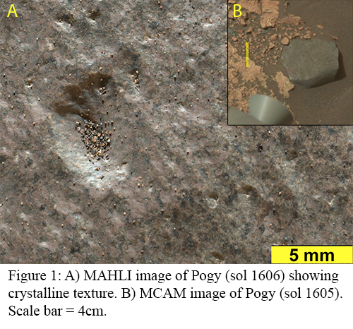
Float Rock Textures: Among the Ireson Hill samples, Pogy shows an unusual texture with two visually distinct phases (Fig. 1). A lighter toned phase makes up ~50% of Pogy’s texture, and the darker toned phase ~10% (measured through pixel counting of manually selected areas), with the remainder being interstitial material without distinct grains. Both phases are anhedral, with grain sizes typically ranging from 1-1.5 mm. The texture appears largely crystalline. It appears notably dissimilar in appearance to the local Stimson in situ and float rocks [5] found at Ireson Hill.
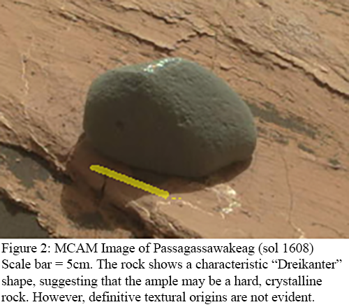
Among the other Ireson Hill targets, Passagassawakeag is an instance of a well-defined Dreikanter, which hints at a harder, crystalline mineralogy (Fig. 2). The remaining targets, Quimby and Wassataquoik do not show such strong evidence for igneous origin in available RMI and Mastcam imagery, but also do not feature the sedimentary texture of surrounding bedrock and float targets, and we therefore include them as possible igneous targets in this analysis.
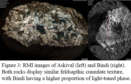
The two remaining targets discussed here, Bindi and Askival, display similar textures to each other. Both rocks display cumulate texture (Fig. 3), with light-toned, subhedral mineral grains with sizes up to >10 mm accounting for the majority (65%-70% in Askival) of the texture and dark toned assemblages (30%-35% in Askival) poikilitically enclosing the light toned grains, as interstitial material. Examples of small dark crystals enclosed within the lighter phase are also present. Askival also displays limited (approx. 1.2%) light toned sulphate emplaced as interstitial material. When combined with chemical analysis (below) of the light-toned grains this identifies these samples as feldspathic cumulates.
Compositions: Results for Pogy are presented SO3-free with a corresponding amount of CaO removed in order to account for excess CaSO4 present on Martian rock surfaces. Results were then recalculated to 100% total weight. Pogy’s APXS geochemical composition (Fig. 4) shows similarity in SiO2, Na2O, K2O, CaO, Al2O3 & TiO2 to the Adirondack-class basalt compositions predominant at the Gusev crater MER mission site, although it has a lower Mg#. However, we note that this similarity does not in itself establish an igneous origin for Pogy as Martian sedimentary rocks can also record igneous source compositions [1,3,5,7].
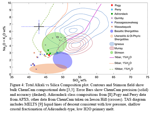
MELTS [4] modelling (Fig. 4) indicates that Pogy-like compositions can be generated by fractionation of magmatic compositions previously derived as parental to Adirondack-class basalts [9], with approximately 13% of the original mass removed through olivine fractionation. The exact conditions of magmatic evolution differ somewhat from the Gusev basalt pathways in order to account for the lower Mg# of Pogy’s composition compared to the Adirondack composition.


Bindi and Askival display clearly feldspathic compositions for a subset of the ChemCam LIBS spots, where the targeted spot was on a light-toned grain. Dark toned grains have mafic compositions. The two targets overall chemistry is differentiated by a higher SiO2 abundance in Askival. Comparing other elemental oxide abundances to SiO2 (Fig. 5 reveals a trend away from the Bindi compositional area, which we interpret as evidence of post-cumulate formation silicification. Comparison of the Albite-Anorthite phase ratio (Fig. 6) between Askival and Bindi shows an overlap, indicating that the cumulates may have formed under similar conditions. We again use MELTS with a variety of input compositions. Modelling performed with the “Johnnie” (basaltic Gale crater target) composition (Fig. 6) produces feldspars with similar phase compositions to those seen in Askival and Bindi.
Conclusions: Ireson Hill float rocks show a variety of textures and compositions, some of which e.g. Passagassawakeag and Pogy appear to be more crystalline than local Stimson bedrock and derived float. Pogy appers to be an igneous, plutonic rock, with an uncertain emplacement process at Ireson Hill.
Comparing to known Gale compositions and rocks, suggests that the Pogy composition represents low pressure, low H2O, fractionation in a shallow crustal setting. This has been preserved either directly as an igneous rock or as a dominant source component in some Gale sedimentary units [5]. The Askival and Bindi float targets are feldspathic cumulates, with Askival’s composition showing evidence for alteration of an original state similar to Bindi. MELTS modelling indicates that these cumulates could have been derived from a source with similar composition to typical Gale crater basalts.
References: [1] Edwards, P.H., et al.,. MAPS, 2017. 52(11): p.2931-2410. [2] Cousin, A., et al. Icarus, 2017. 288: p.265-283. 113622 [3] Bedford, C.C., et al.,. GCA, 2019. 246: p.234-266. [4] Ghiorso, M.S. et al. Eos, Trans AGU, 1994. 75(49): p.571-576. [5] Bedford, C.C., et al., Icarus, 2020. 341 [6] Yen et al., EPSL, 2017, 471: p.186-198 [7] Siebach, K.L., et al., Journal of Geophysical Research: Planets, 2017. 122(2): p.295-328. [8] McSween, H.Y., et al.. Science, 2004. 305: p.842-845. [9] Filiberto, J. and R. Dasgupta, EPSL, 2011. 304(3): p.527-537.
How to cite: Bowden, D., Bridges, J., Cousin, A., Schwenzer, S., Wiens, R., Gasnault, O., Thompson, L., Gasda, P., Bedford, C., Turner, S., and Williams, R.: Igneous Float Rocks at the Ireson Hill and Bressay Localities, Gale Crater, Mars, Europlanet Science Congress 2020, online, 21 Sep–9 Oct 2020, EPSC2020-861, https://doi.org/10.5194/epsc2020-861, 2020.
Introduction: Small cones are common on Mars [1]. Some are concentrated in large fields or form long chains of several dozen kilometers long. Similar cones and chains are observed on Earth in volcanic zones (e.g., Iceland).
The origin of cones on Mars is discussed in many papers [e.g., 2-5]. [2] investigated cones in Chryse Planitia. They believe that the cones are mostly results of mud volcanism and/or evaporite deposition.
Considered region: We analyzed the region on Chryse Planitia centered in ~38o13’ N and ~40o35’W - Figs 1 and 2. The region is at the boundary of a smooth plain (AHcs) and a complex unit (AHcc). AHcs is the Amazoniam-Hesperian smooth plain. A small region of another type (HNck in Fig.1) is: “older knobby material” [6]. All of considered forms are composed of lacustrine deposits. They are thick enough to cover possible underlying wrinkle ridges – [6]. These ridges could be a source of hot lava or pyroclastic falls.
Figure 1
Our region under study at Chryse Planitia (the white square) is at the boundary of smooth plain (AHcs) and complex unit (AHcc). HNck is the “older knobby material” – [6].

Figure 2
The considered region (see also Fig. 1). The chains of cones are indicated by solid black arrows and labeled by numbers 1, 2, 3, 4, 5. According to our hypothesis, the chains are formed along outcrops of sediment layers with high content of volatiles.
Proposed mechanisms of formation of chains: Our hypothesis assumes that the investigated region had been covered with several layers of lacustrine deposits with the layers of sediments rich in volatiles separated by layers with small amount of volatiles – Fig. 3.

Figure 3
The scenario, leading to formation chains of cones. Legend:1 – rich volatiles deposits, 2 - fissures, 3 – low volatile deposits, 4 – cones.

Figure 4
Apparent Thermal Inertia (ATI) map calculated from three pairs of THEMIS thermal bands (I11560003-I36037011, I47513003-I05775011 and I11560003=I36037011) and CTX based albedo (CTXP19_008417 - gray scale image).
Apparent thermal inertia (ATI):
It approximates thermal inertia and is often useful in remote sensing – Fig.4. The fundamental equation is ATI=(1-A)/∆T, where ΔT is the diurnal temperature difference (in K), and A is the Lambertian albedo. ΔT is obtained from THEMIS images (in this study: I11560003-I36037011). Albedo is derived from CTX images. Geometric, topographic and atmospheric corrections are applied. The ATI values range from 397.3 to 1134.4 with the arithmetic mean of 510.6 and median value of 496.9 J m-2 K-1 s-1/2. These values indicate the presence of sand and gravel.
Hypothesis of mud volcanoes:
. The ‘Martian version’ of mud volcanism could be substantially different than its terrestrial counterpart [7]. Note first, that the temperature of the boiling water on Mars was (for most of its history) substantially lower than in terrestrial atmosphere. We have assumed that some sedimentary layers contained substantial amount of water or ice. The stability of these layers depends on the pressure. A fissure, extending from the surface of Mars to the layer containing volatiles, could lead to the drop of pressure and release of gases. The gas release had led to development a chain of conical structures along the outcrop – Fig. 3.
Hydrocarbon stored in clathrates could be important for this process. The clathrates could release volatiles along outcrops at the temperature substantially lower than temperature of water. Probably, on Earth there have never been similar global processes (see however [8]).
Hypothesis of rootless cones:
The size and shape of the considered cones are not substantially different than many terrestrial rootless cones. The rootless cones are often generated when hot lava is interacting with water or ice. If lava flows through glacier or wetlands then it produces explosive outgassing. The blisters of water vapor could break through the lava and cause a so-called hydro-volcanic explosion, eventually forming pseudo-craters. Because the lava cools quickly, it does not spill around the cone.
Terrestrial rootless cones are of the shape and size similar to the cones on Chryse Planitia. The scenario leading to the origin of rootless cones in the considered region of Chryse Planitia requires the interaction of volatile-rich deposits from the outcrops with some hot matter. This hot matter could be a result of a rejuvenation of volcanic processes in a ridge adjacent to the considered area.
Conclusions:
1.We have presented the hypothesis explaining the origin of the cones chains in the chosen region of Chryse Planitia.
2.1 The ‘mud volcano mechanism’ assumes that the volatiles in the sediment layer are warm enough to be unstable. High temperature can be a result of increased heat flow of late magma intrusion below lacustrine deposits.
2.2 The ‘rootless cones mechanism’ requires hot volcanic material to come into contact with volatile-rich sediments.
Acknowledgments: This study was supported by statutory project of Institute of Geophysics of University of Warsaw.
References:
[1] Frey H., and Jarosewich, M., (1982) J. Geophys. Res. 87, 9867-9879. [2] Fagents, S., and Thordarson, T., (2007) https: //www.researchgate.net/publication /252418640._ [3] Farrand, W. H., et al., (2005), J. Geophys. Res.,110, E05005. [4] Gallinger, C.L. and Ghent, R.R,. (2016) 47th LPSC 2767.pdf. [5] Ghent, R. R., et al. (2012) Icarus 217, 1, 169-183. [6] Rotto, S., and K. L. Tanaka, (1995) Geologic/geomorphologic map of the Chryse Planitia: region of Mars. USGS. [7] Allen, C. C.; et al. (2008) Astrobiology, 8, 6, 1093-1112. [8] Allen. C.C., et al., (2013) Icarus 224, 424–432. [9] Orosei, R., et al., (2018). Science, vol. 361, 6401, 490-493. [10] Brož, P., et al., (2014) Earth and Planet. Sci. Let. 406, 14-23.
How to cite: Czechowski, L., Zalewska, N., Zambrowska, A., Ciazela, M., Witek, P., and Kotlarz, J.: Mechanism of Origin of Chains of Cones in Cryse PLanitia , Europlanet Science Congress 2020, online, 21 Sep–9 Oct 2020, EPSC2020-895, https://doi.org/10.5194/epsc2020-895, 2020.
1. Introduction
In 2008, the High Resolution Imaging Science Experiment (HiRISE) on board NASA’s MRO fortuitously captured several discrete clouds of material (Fig.1) in the process of cascading down a steep scarp of the water-ice-rich north polar layered deposits (NPLD). The events were only seen during a period of ~4 weeks, near the onset of northern spring, when the seasonal cover of CO2 is beginning to sublimate from the north polar regions. Russell et al. [1] analyzed the morphology of the clouds, inferring that the particles involved were mechanically analogous to terrestrial “dry, loose snow or dust”, making the events similar to terrestrial “powder avalanches” [2]. HiRISE confirmed the seasonality of these avalanches the following spring, and has been monitoring them (Fig.2) for a total of 7 Mars Years (MY29–MY35). We will present observations from this monitoring. We seek to: (1) quantify the frequency of these events (2) quantify their effect on the mass balance of the NPLD (especially with respect to competing processes such as viscous deformation and other mass-wasting events [3-5], and (3) investigate possible trigger mechanisms.
2. Observations
The avalanches often appear as dense clouds of reddish, air-lofted material moving down scarps of the NPLD margins. The scarps are steep (>50º) and appear fractured (Fig.1), and the clouds themselves range in extent from just a few tens of meters to over 200 m. Observations of many avalanche events at different stages allow us to deduce the course of a typical event. Avalanches start at a discrete point on the steep face and remain small and optically thick as they descend (Fig.1a,b). Upon reaching the basal unit they spread outward at speeds of several m/s (measured from color fringing in HiRISE images [1]), become optically thinner, and develop a more diffuse boundary (Fig1.c,d). The avalanches then transition to near-stationary clouds close to, but detached from the scarp, which presumably slowly settle onto the exposed basal unit (Fig.1e).
A total of 57 events have been captured in action on the so-called “Discovery Scarp” (Fig.2) since the first five events were captured here in a single HiRISE image. On average, 8 events are captured on this scarp per year, and they tend to occur on its steepest sections (50–70º), and preferentially on SW-facing scarps. Figure 2 shows the location of the Discovery Scarp and all other scarps along the NPLD margins where avalanches have been observed. An average of 20 new events are observed every year.
Avalanches have only been observed to occur between Ls 5º and 70º, and thus are an exclusively “springtime” event. This time of year coincides with both the sublimation of seasonal CO2 ice over the north polar region, and with a peak in subsurface compressional stresses in the scarp walls, as shown by [6].
3. Trigger mechanisms
In accordance with the seasonality of the avalanches, trigger mechanisms to consider are (1) sublimation-driven collapse of sections of the scarp wall (material in the avalanches would most likely be a combination of CO2 and surface dust), and (2) thermal stress-driven collapse, similar to exfoliation of granitic domes on Earth [6] (material would mostly be pulverized dusty water ice, i.e. the material that makes up NPLD beds).
To examine the first mechanism, we acquired HiRISE images early in the season, before the events occurred. Images of the discovery scarp at Ls 350º (Fig.3a) and Ls 1º appear to show that the CO2 has already sublimated from the steepest parts of the wall by this time. However, CRISM spectra of this location (Fig.3b,c) show absorption bands diagnostic of CO2 until after Ls 50º. Though the bands are weak, their presence suggests CO2 persists until this time. We also used a 1D thermal balance model [7] to calculate the amount of CO2 frost that accumulates on a steep surface throughout the year. With conservative estimates for thermal properties (i.e., assumed an exposed wall of water ice), model results show that on a 50º SW-facing slope, all CO2 frost has sublimated by Ls 10º, matching HiRISE observations but contradicting CRISM. This thermal model is extremely sensitive to dust cover on the scarp wall however, and a few cm of dust can accumulate, and maintain wintertime CO2. It is also possible that the steepness of the scarp makes it difficult to isolate in the CRISM data, and that the absorption bands correspond to influence from adjacent, flatter terrains.
4. Results and Future Work
Our study shows that north polar cap avalanches occur frequently on steep, marginal scarps of the NPLD, and likely have a substantial effect in eroding the NPLD. There are contradicting observations of CO2 frost on the steepest areas of the scarps, which we will further investigate with CRISM observations at high-roll angles that view the scarp more head-on. Even if CO2 is present in small amounts on the scarps early in the year, we have found that it is the fractured scarps that show a much higher frequency of avalanches than those that show little to no fracturing. Thus, although CO2 may be present in the clouds mixed with the avalanche material as it moves over the basal unit, a more likely trigger seems to be the springtime peak in compressional stresses that fractures the scarps [6]. In the future, we will quantify the mass wasted by the events with flow models used for terrestrial processes, and further investigate the triggers with improved detail in the thermal and stress models.
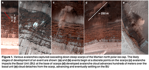
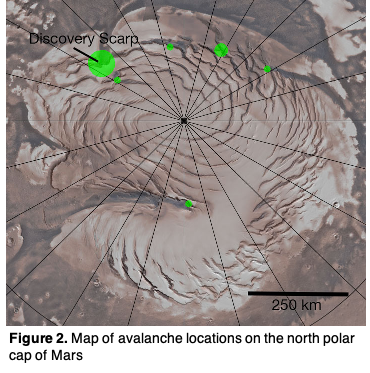
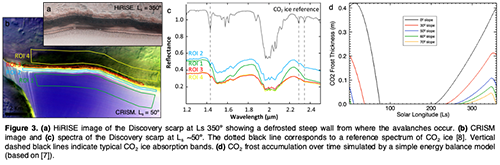
References
[1] Russell et al. (2008) GRL. 35, L23204. [2] McClung and Schaerer (2006), Mountaineers, Seattle Wash. [3] Sori, et al., GRL, 43. [4] Herkenhoff et al. (2020) 7th ICMPSE [5] Fanara et al. 2020, Icarus [6] Byrne et al. (2016), 6th ICMPSE [7] Dundas and Byrne (2010) Icarus 206, 716.
How to cite: Becerra, P., Herny, C., Valantinas, A., Byrne, S., Thomas, N., and Conway, S.: Avalanches of the Martian north polar cap, Europlanet Science Congress 2020, online, 21 Sep–9 Oct 2020, EPSC2020-1093, https://doi.org/10.5194/epsc2020-1093, 2020.
Magnetic pulsations are observed at Mars in the magnetotail and on the surface by the Maven and InSight magnetometers. The surface observations exhibit a frequency-dependent polarization in which the amplitude of the vertical component weakens with increasing frequency. This frequency dependence is not seen in the source regions studied by MAVEN. The source of the frequency dependence must be in the subsurface of Mars. The attenuation is consistent with an aquifer that is 3 km thick, containing water of the conductivity of terrestrial seawater.
How to cite: Yu, Y., Luhmann, J., and Russell, C.: Martian Aquifers: Detection by Magnetic Sounding from Surface Magnetometry, Europlanet Science Congress 2020, online, 21 Sep–9 Oct 2020, EPSC2020-169, https://doi.org/10.5194/epsc2020-169, 2020.
Introduction
On Mars, polygonally patterned ground is widespread at the mid to high latitudes and it is accepted to result from thermal contraction of ice-cemented soil1. Low-centered polygons (LCPs), i.e. polygons with a relatively lower elevation at their centre (Figure 1a), and high-centered polygons (HCPs), i.e. polygons with a relatively higher elevation at their centre (Figure 1b), can be observed at the martian mid latitudes2.
On Earth, ice-wedge polygons are morphologies that are formed when ice aggrades on a seasonal basis in thermal contraction cracks in ice-cemented soil3. This aggradation uplifts the sediment at the polygon margins forming LCPs. When ice-wedge polygons degrade as mean seasonal temperatures rise, the melting of the ice in the wedges drops the elevation at the polygon margins, forming HCPs3.
Both LCPs and HCPs can also be formed when the wedge-material is wind-blown sand, rather than ice; however, were the wedges comprised of sand a variance in morphology based on a change of latitude would not be expected since in this case the type of polygon expressed should not depend on the ambient thermal conditions. Therefore, based on the assumption that ground ice stability increases poleward on Mars4, we hypothesise that the relative abundance of LCPs compared to HCPs should increase with latitude if these polygons are a result of ice wedges rather than sand wedges. We test this hypothesis in a region of Utopia Planitia (Figure 2), where there is good coverage of high-resolution images sufficient to distinguish LCPs from HCPs and the widespread occurrence of polygonally patterned ground5.
Method
We used 73 High Resolution Imaging Science Experiment (HiRISE) images at 25-50 cm/px over the Utopia Planitia study region (Figure 2). 59 images remain to be analysed for a total of 132. The study area was divided into squares of 250,000 km², and for each one the presence or absence of LCPs and HCPs in the images was noted – where there were overlapping images only the highest quality image was assessed. At least five LCP- or HCP-type polygons must occur per square for their presence to be noted. Images were divided into two groups: the ones whose resolution/quality allows unambiguous identification of LCPs and/or HCPs when present (47 images, 29 with polygons), and the ones where identification was more challenging (26 images, 20 with polygons) e.g. because of low resolution, small polygon sizes, poor contrast, and/or atmospheric haze. Three further images were of insufficient quality for analysis. We distinguished two types of host terrain: “craters” (≥ 2 km diameter) and inter-crater plains. Finally, the ratio of the number of LCPs to the number of HCPs was calculated for each degree of latitude for both terrain types, and also for each image.
Results
We compared the data from the low resolution/quality images to the higher resolution/quality images and found the same latitudinal trends in the LCP-to-HCP ratio. We therefore considered these images as having reliable data, and results from both groups are reported in the subsequent analysis. In Figure 2 we show the LCP-to-HCP ratio per HiRISE image, however below and in Figure 3 we report the LCP-to-HCP ratio calculated for every 1° of latitude no matter which image they fall within.
If the LCP-to-HCP ratio is plotted for the polygons in craters and on the plains separately, polygons located on the inter-crater plains show a strong correlation between latitude and LCP-to-HCP ratio (R² ≈ 0.86, p-value ≈ 0.0003; Figure 3). Note that the LCP-to-HCP ratio is nearly always higher in craters than it is on the plains particularly at lower latitudes. However, no latitudinal trends are observable in the LCP-to-HCP ratio for polygons in craters (R² ≈ 0.12; Figure 3). Note that the extreme value of 6 in the LCP-to-HCP ratio at 40°N originates from two 30-40 km craters in which LCPs are very common and at this latitude no other HiRISE image with polygons has been found. When the data are analysed as an ensemble (i.e. the host terrain type is not taken into account), we find no correlation between latitude and LCP-to-HCP ratio (R² ≈ 0.28).
Conclusions
- polygons located on the plains in Utopia Planitia show a positive correlation between latitude and LCP-to-HCP ratio that is statistically strong. This provides evidence in support of the hypothesis that these polygons have ice-wedges at their margins whose degradation increases towards the equator1.
- the LCP-to-HCP ratio of polygons inside craters does not show any trend with latitude. We suggest that the micro-environment inside the crater could protect the ice-wedges from degradation: craters could form cold traps where volatiles are preferentially preserved6. This is supported by the higher LCP-to-HCP ratio in craters compared to the plains and the occurrence of polygons in craters to lower latitudes than on the surrounding plains. Our next step will be to examine the other factors that could influence the type of polygon that occurs inside craters, including elevation, crater diameter and preservation state.
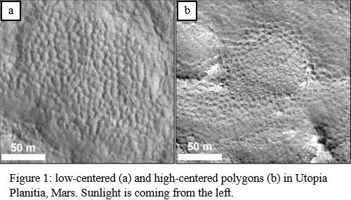
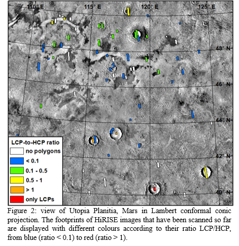

References
1Mellon M.T. (1997) J. Geophys. Res. 102 (E11), 25,617–25,628.
2Soare R.J. et al. (2018) Chapter 7, in, Dynamic Mars, recent landscape evolution of the red planet, eds. Soare, R.J., Conway, S.J. and Clifford, S.M., Elsevier, 464 p.
3Lachenbruch A.H. (1962) GSA Special Paper 70. vol. 69 Geological Society of America, New York.
4Schorghofer N., Forget, F. (2012) Icarus 220, 1112-1120.
5Soare R.J. et al. (2020) Icarus 342, 113233.
6Conway S.J. et al. (2012) Icarus 220, 174-193.
How to cite: Soare, R. J., Philippe, M., Conway, S. J., Williams, J.-P., Mc Keown, L. E., Godin, E., and Hawkswell, J.: Possible ice-wedge polygonisation in Utopia Planitia, Mars and its poleward gradient of latitude, Europlanet Science Congress 2020, online, 21 Sep–9 Oct 2020, EPSC2020-385, https://doi.org/10.5194/epsc2020-385, 2020.
Please decide on your access
Please use the buttons below to download the presentation materials or to visit the external website where the presentation is linked. Regarding the external link, please note that Copernicus Meetings cannot accept any liability for the content and the website you will visit.
Forward to presentation link
You are going to open an external link to the presentation as indicated by the authors. Copernicus Meetings cannot accept any liability for the content and the website you will visit.
We are sorry, but presentations are only available for users who registered for the conference. Thank you.