Oral presentations and abstracts
This session welcomes all presentations on Mars' interior and surface processes. The aim of this session is to bring together disciplines as various as geology, geomorphology, geophysics, mineralogy, glaciology, and chemistry. We welcome presentations on either present or past Mars processes, either pure Mars science or comparative planetology, either observations or modeling or laboratory experiments (or any combination of those). New results on Mars science obtained from recent in situ and orbital measurements are particularly encouraged, as well as studies related to upcoming missions (ExoMars, Mars 2020, Mars Sample Return).
Session assets
While liquid water is not thermodynamically stable at the surface due to the low temperature and pressure conditions, liquid groundwater may still exist in the Martian subsurface [1, 2].
In this study, we use fully dynamical 3D thermal evolution models [3] and 3D parametrized models [4] to calculate the depth at which favorable conditions for liquid water are present, assuming that a global subsurface cryosphere exists on Mars today. While fully dynamical 3D models take into account the effect of mantle plumes self-consistently, they are computationally expensive compared to 3D parametrized models that can cover a large range of mantle conditions, although requiring additional parametrizations for thermal anomalies in the interior. In all calculations, we use a 3D crustal model that is compatible with today’s gravity and topography data [5, 6].
Some of the most important parameters that affect the depth of liquid water are the spatial variations of crustal thickness and crustal thermal conductivity, since the crust has a lower thermal conductivity compared to that of the mantle and thickness variations can shift the groundwater table locally closer to the surface (Fig. 1). The amount and distribution of heat sources, and the presence of mantle plumes, can introduce additional perturbations to the depth of groundwater. The surface temperature distribution and the presence of salts and clathrate hydrates considerably affect the depth and locations where subsurface liquid water may be stable. Hydrated magnesium (Mg) and calcium (Ca) perchlorate salts, whose presence has been suggested at various locations on Mars [7], may significantly reduce the melting point of water ice. In addition to thick regolith layers, clathrate hydrates, if present in the subsurface, would provide an insulating effect reducing the crustal thermal conductivity at least locally [e.g., 8].
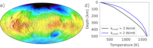
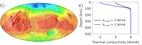
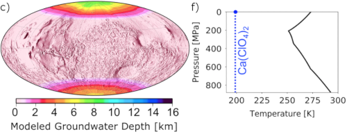
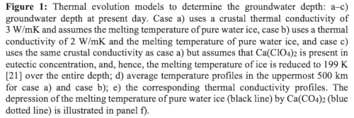
The effects of the crustal thermal conductivity and salt abundance on the depth of subsurface liquid water are shown in Fig. 1, where we use the same crustal thickness variations and crustal enrichment in radioactive heat sources in all simulations. The model in Fig. 1a assumes an average crustal conductivity of 3 W/mK, while the model in Fig. 1b has a lower conductivity of only 2 W/mK (see panel 1e for the spatially averaged conductivity profiles that, due to crustal thickness variations, show average values between mantle and crust in the topmost 110 km). Fig. 1d shows the effect of the crustal thermal conductivity on the subsurface temperature profile. For the lower conductivity case the subsurface temperature is warmer, and the groundwater table shifts, on average, 2.5 km closer to the surface. The model shown in Fig. 1c is similar to the one in Fig. 1a but assumes the presence of salts. Instead of using the melting temperature of pure water ice, as was done for the models in Fig. 1a and b, we lower the melting temperature to 199 K [9] over the entire depth, by assuming that Ca(ClO4)2 is present in eutectic concentration (Fig. 1f). This extreme, and unrealistic, assumption places constraints on the minimum depth at which liquid water may be present in the Martian subsurface today, since kinetic factors such as the flow of groundwater due to gravity may increase the depth of the water table, depending on the total amount of liquid water, porosity and permeability.
In Fig. 1a and b, the depth of the groundwater shows the combined effect of crustal thickness distribution and surface temperature variations. Mantle plumes have only a small effect and may introduce perturbations only if the groundwater is located, on average, at about 5 km depth or deeper. The effect of the crustal thickness is evident in basins, along the dichotomy, and in volcanic provinces, whereas surface temperatures give general water table depth trends with latitude. In Fig. 1c, the depth variations of the groundwater table are mainly caused by the surface temperature distribution, as the groundwater table is located very close to the surface (between 0 – 1 km for latitudes between -57° and 57°). Nevertheless, in all cases (Fig. 1a – c), the water table is significantly shallower in equatorial regions compared to polar regions, mainly governed by lower surface temperatures at the poles.
Our results suggest that the Martian subsurface has had, and still has, the potential to enable deep environments with stable liquid groundwater. Combined with the analysis of geomorphological features at the Martian surface that testify the involvement of water/ice activity and maps of subsurface water ice [10], such models could provide valuable estimates of the depth of liquid groundwater on past and present-day Mars providing key knowledge on the planet dynamics, evolution and astrobiological potential.
The technology to probe the Martian subsurface at depths of many kilometers is maturing [2]: TH2OR (Transmissive H2O Reconnaissance), a low-mass and average low-power transient electromagnetic sounder capable of detecting the presence of liquid water to depths of many kilometers is currently being developed at JPL [11]. Moreover, mission concepts such as VALKYRIE (Volatiles And Life: KeY Reconnaissance & In-situ Exploration) [12], which would add to the liquid water sounder a drill capable of accessing depths of 10s-100s of meters or more and employ a (bio)geochemical analysis package on the surface, would provide the measurements necessary to characterize the modern-day subsurface habitability of Mars.
References: [1] Clifford et al., 2010, JGR, 115(E7); [2] Stamenković V. et al., 2019, Nat. Astron., 3(2); [3] Plesa A.-C. et al., 2018, GRL, 45(22); [4] Breuer D. & Spohn T., 2006, PSS, 54(2); [5] Plesa A.-C. et al., 2016, JGR, 121(12); [6] Wieczorek M. & Zuber M., 2004, JGR, 109(E8); [7] Leshin L. et al., 2013, Science, 341; [8] Kargel J. et al. 2007, Geology, 35(11); [9] Marion G. et al., 2010, Icarus, 207(2); [10] Piqueux S. et al., 2019, GRL, 46.; [11] Burgin M. et al., 2019, AGU Fall Meeting, P44B-02; [12] Mischna M. et al., 2019, AGU Fall Meeting, P41C-3466.
Acknowledgments: This work was performed in part at the Jet Propulsion Laboratory, California Institute of Technology, under contract to NASA. © 2020, California Institute of Technology.
How to cite: Plesa, A.-C., Stamenković, V., Breuer, D., Hauber, E., Tarnas, J., Mustard, J., Mischna, M., and De Toffoli, B. and the TH2OR and VALKYRIE Teams: Mars' Subsurface Environment: Where to Search for Groundwater?, Europlanet Science Congress 2020, online, 21 Sep–9 Oct 2020, EPSC2020-698, https://doi.org/10.5194/epsc2020-698, 2020.
Abstract: Calcium sulfate mineral veins cross-cut fluviolacustrine sedimentary rocks at many localities on Mars. Although these veins probably formed under habitable conditions, their potential to retain ancient biosignatures is poorly understood. Here, we report ancient biogenic authigenic pyrite (FeS2) lining a fibrous gypsum (CaSO4.2H2O) vein of probable Cenozoic emplacement age from Permian lacustrine rocks in Northwest England. The observed pyrite distributions and textures suggests that the pyrite formed replacively after gypsum within the veins and was not inherited from the host rock. Spatially resolved ion microprobe (SIMS) measurements reveal that the pyrite sulfur isotope composition (δ34SVCDT) is negatively offset from the host gypsum by ~40‰. We infer that the pyrite was precipitated in the deep subsurface by microorganisms living in porosity at the vein margins, which coupled the reduction of vein-derived sulfate to the oxidation of wall-derived organic matter. This implies that such veins can incorporate biosignatures that remain stable over geological time, which could in principle be detected in samples returned from Mars [1].
Introduction: Fibrous, antitaxial calcium sulfate veins were encountered by the MER rover Opportunity in Endeavour Crater and are inferred to represent gypsum [2,3]. Similarly, white calcium sulfate veins (anhydrite, bassanite, and perhaps gypsum) cross-cut hundreds of metres of fluviolacustrine and aeolian stratigraphy traversed by the MSL Curiosity rover in Gale Crater, including the Yellowknife Bay and Murray formations [4,5,6,7]. Some of these veins are thought to post-date lithification and to have formed at depths of over 1 km in the subsurface [8]. Veins like these may be encountered in future by the Perseverance and Rosalind Franklin rovers, and have sometimes been discussed as an attractive target for astrobiological investigation, but their potential to preserve biosignatures is poorly understood. Here, we summarise a new study [1] of ancient biosignatures in ancient (Cenozoic), bedding-parallel, antitaxial veins of white, fibrous gypsum found in Permian lacustrine mudrock. These veins are located in the Eden Shales Formation of the Vale of Eden Basin, Cumbria, NW England, and were sampled underground in situ in the Kirkby Thore gypsum mine.
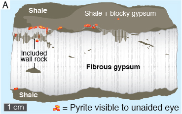
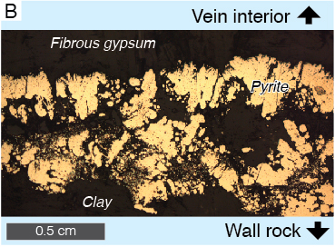
Figure 1: Pyrite at the margins of a gypsum vein. A: Sketch of hand sample. B: Reflected light photomicrograph showing brassy pyrite with complex microdigitate morphology at gypsum vein margin.
Results: Pyrite was observable to the unaided eye at the margins of the gypsum veins in polished hand samples (Figure 1A); its composition was confirmed with energy-dispersive X-ray spectroscopy. The pyrite displays a complex interfingering boundary with the surrounding gypsum, suggestive of replacive authigenic growth (Figure 1B; we do not consider this morphology itself a biosignature). Gypsum-entombed carbonaceous material of probable organic origin was identified by Raman spectroscopic microscopy in close proximity to the pyrite (from its prominent D- and G-bands); authigenic dolomite is also present. Spatially resolved ion microprobe (SIMS) measurements reveal that the pyrite sulfur isotope composition is consistently very light (δ34SVCDT = –30.7 ‰). Comparison with the sulfate in the vein gypsum (δ34SVCDT = +8.5 ‰; [9]) indicates a fractionation too large to be explained by non-biological (thermochemical) sulfate reduction (which in any case would be difficult to reconcile with the burial history of the host rock). We infer from these results that the pyrite is likely a product of in situ microbial sulfate reduction coupled to the oxidation of organic matter from the wall rock.
Implications for Mars: Our results imply that the porous margins of calcium sulfate veins in the subsurface can serve as conduits for the flow of sulfate-rich groundwater, and therefore as potential habitats for prokaryotes capable of utilizing this sulfate to oxidize organic carbon. Such habitats may disappear and reappear several times over long spans of geological time as veins reopen under changing stress regimes and re-seal as further sulfate precipitates. Microbial sulfate reduction in our samples was probably stimulated by the low but appreciable organic content of the host rock (TOC ~ 0.5 wt%). Other sources of carbon (e.g., methane) and electrons (e.g., hydrogen) may be available in organic-poor rocks on Mars. In principle, signatures of subsurface life similar to those reported here could be detectable in martian veins, particularly if they were selected to be returned to Earth for SIMS analysis. On Earth, the δ34S biosignature has been identified in rocks as old as 3.47 Ga, although it did not become widespread until after 2.5 Ga [10,11]. Sulfur isotope systematics are not well understood in martian contexts, and the isotopic fingerprints of any indigenous martian organisms may well have differed from those of life on Earth. Nevertheless, sulfide minerals do occur on Mars, and Curiosity Rover has detected isotopically light sulfide (by evolved gas analysis) in Gale Crater sediments, where it could ultimately have originated either from abiotic or from biotic processes [12]. The presence of preserved organic matter in our samples adds to the case that calcium sulfate veins could be an attractive target for analysis on Mars. We note that any biosignatures present in mineral veins cross-cutting sedimentary rocks would have originated in a subsurface habitat markedly different from the depositional environment of the host mudrock. As sampling targets, these rocks may therefore offer insights into two ancient martian habitats — surface and subsurface — for the price of one.
References: [1] McMahon, S., Parnell, J., & Reekie, P.B.R. Astrobiology (accepted). [2] Squyres, S.W., et al. (2012). Science 336:570–576. [3] Arvidson, R.E., et al. (2014). Science 343:1248097. [4] Nachon, M., et al. (2014) J Geophys Res Planets 119:1991–2016. [5] Vaniman, D.T., et al. (2014) Science 343:1243480. [6] Kronyak, R.E., et al. (2019) Earth Space Sci 6:238–265. [7] Minitti, M.E., et al. (2019) Icarus 328:194–209. [8] Caswell, T.E., and Milliken, R.E. (2017) EPSL 468:72-84. [9] Armstrong, J., et al. (2020) Ore Geology Reviews 116: 103207. [10] Shen, Y., et al. (2009) EPSL 279:383–391. [11] Thomazo, C., et al. (2009) Comptes Rendus Palevol 8:665–678. [12] Franz, H.B., et al. (2017) Nat Geosci 10:658–662.
How to cite: McMahon, S., John, P., and Philippe, R.: Mars-analogue calcium sulfate veins record evidence of ancient subsurface life, Europlanet Science Congress 2020, online, 21 Sep–9 Oct 2020, EPSC2020-1049, https://doi.org/10.5194/epsc2020-1049, 2020.
The Axius Valles on the Malea Planum region’s (MPR) northern flank down into the Hellas basin are one of the most extensive and densest channel networks on Mars [1,2]. While previous studies tentatively interpreted the area as pyroclastic deposits dissected by sapped water/lahar flows [3-8] we considered their viability versus low-viscosity lava flows.
Physiography
The Axius Valles and adjacent channels to the west consist of ~22,550 km of mostly parallel sinuous valleys dissecting a plain (drainage density of 0.09 km-1) of gentle but relatively uniform northnortheast tilt, i.e., long-wavelength dip, at ~0.6 to 0.9° (~1 to 1.6%) towards the Hellas basin floor. The channels are up to ~20 km wide and ~100 m deep, although most are narrower and shallower than ~5 km and ~50 m, respectively. The majority of the valleys originates around the rim of Amphitrites Patera between elevations of ~1,200 and ~1,600 m. Smaller subsets originate at or below the rim of Peneus Patera between elevations of ~0 m and ~600 m, or are traceable further south into the wrinkle-ridged plains of the MPR. The longest continuously traceable valley of the Axius Valles is ~325 km long and follows the topographic gradient from ~600 m above the datum down to ~ -4,800 m. The valleys’ sinuosity is relatively low, ranging from ~1 up to ~1.15, and anabranching is very common. In several locations, sinuous valleys are levéed, i.e., bound by ridges that can be up to ~100 m high.
Discussion
Based on their morphology and location, the Axius Valles have been tentatively interpreted as the result of sapped water or lahar flows that carved into friable pyroclastic deposits [3-7]. However, diagnostic features such as short, digitate levée-overspill deposits, bulged, lobate flow fronts (both typical for high viscosity flows, i.e., most lavas or mud/sludge), and associated pit-chains (typical for lava tubes, i.e., lava flows) are absent but might have been covered by 10s of meters thick dust-ice mantling [12] or eroded by intense deflation [e.g., 13]. In any case, the fact that the channels extend over 100s of kilometers on a slope of <1° seems to favor low viscosity density currents. Water or sludge flows stand to reason especially as ice accumulation models for an ancient martian 1 bar atmosphere predict a several 10s of meters thick ice sheet, i.e. potential melt water source, to form on the highest points of Amphitrites Patera [14]. Nevertheless, due to the geographic association with this patera – likely one of the largest calderas on Mars [e.g., 11,15] – the plausibility of very low-viscosity lavas such as komatiite and tholeiitic basalt [16-18] as alternatives to water should be ascertained. Mantle-derived low-viscosity magmas such as komatiite or tholeiitic basalt [e.g., 19-21] are indicated by the broad and gently sloped shields of Amphitrites and Peneus Paterae (11,15,21] and also an expected product of MPR volcanism, which was likely caused by deep ring-fractures and mantle upwelling related to the Hellas basin-forming event [11,15]. Furthermore, models indicate that komatiite and tholeiitic basalt flows on very shallow slopes should be able to travel up to ~325 km and form ~100 m deep channels if flow durations and 2-dimensional discharge rates are at least several months and ~150 m2 s-1, respectively [22,23]. In the channels close to the patera summits, whose average width is ~3 km, this would result in a discharge rate of 450,000 m³ s-1, which is within the spectrum deduced for other large terrestrial, lunar, and martian flows [24,25]. Given the sizes of Amphitrites and Peneus Paterae as potential source areas, as well as the volume of potentially basaltic material filling the Hellas basin (~106 km3 [13]), such discharge rates might be feasible, especially as itwould be a peak value and not constant over the course of a months-long eruption. Lastly, as is the case for overlapping and interacting lava channels on Earth, e.g., on the flanks of Etna or Teide, such networks form sequentially and not all at once, thereby suggesting a volcanic formation of the Axius Valles would have included multiple eruptions, too.
Preliminary Conclusions
The primary parameters of the Axius Valles, i.e., their sinuosity, size, anabranching, levées, and drainage density are not diagnostic and could be explained by multiple types of density currents. The channels’ length over a gentle slope implies low-viscosity liquids, i.e., water/sludge or certain lavas. Most of the channels can be traced back to Amphitrites Patera (likely one of Mars’ largest calderas) and large volumes of low-viscosity lavas are indicated by the area’s morphology. Although water/sludge flows remain a viable alternative to lava, previously proposed groundwater/-ice sapping [7] would not be expected in the hydrogeologically constrained setting of a caldera summit. An alternative is volcanically-induced melting of an ice sheet, which models [14] suggest to have accumulated on Amphitrites Patera in an ancient 1 bar atmosphere.
References
[1] Hynek et al. (2010). JGR: Planets, 115(E9), 1–14. [2] Alemanno et al. (2018). ESS, 5(10), 560–577. [3] Tanaka & Scott (1987). USGS IMAP 1802. [4] Tananka & Leonard (1995). JGR: Planets, 100(E3), 5407–5432. [5] Leonard & Tanaka (2001). USGS Geol. Inv., 2694, 80225. [6] Moore & Wilhelms (2001). Icarus, 154(2), 258–276. [7] Tanaka et al. (2002). GRL, 29(8), 1–4. [8] Bernhardt et al. (2016). Icarus, 264, 407–442. [9] Bernhardt & Williams (2019). Ann. M. of Plan. Geol. Mappers#7013. [10] Bernhardt et al. (2019). LPSC#1435. [11] Williams et al. (2009). PSS, 57(8–9), 895–916. [12] Willmes et al. (2012). PSS, 60(1), 199–206. [13] Bernhardt et al. (2016). JGR: Planets, 121(4), 714–738. [14] Fastook & Head (2015). PSS, 106, 82–98. [15] Peterson (1978). LPSC, 3411-3432. [16] Reyes & Christensen (1994). GRL, 21(10), 887–890. [17] Greeley et al. (2005). JGR, 110(E5), E05008. [18] Williams et al. (2005). JGR: Planets, 110(5), 1–13. [19] Williams et al. (2000). JGR: Planets, 105(E8), 20189–20205. [20] Elkins Tanton et al. (2001). Geology, 29(7), 631. [21] Arndt et al. (2008). Komatiite. ISBN 9780511535550. [22] Huppert & Sparks (1985). J. of Petrol., 26(3), 694–725. [23] Komatsu et al. (1992). GRL, 19(13), 1415–1418. [24] Whitford-Stark (1982). ESR, 18(2), 109–168. [25] Cattermole (1987). JGR: Solid Earth, 92(B4), E553–E560.
How to cite: Bernhardt, H. and Williams, D. A.: Water and lava both seem viable for the formation of one of Mars' densest and largest channel networks, Europlanet Science Congress 2020, online, 21 Sep–9 Oct 2020, EPSC2020-19, https://doi.org/10.5194/epsc2020-19, 2020.
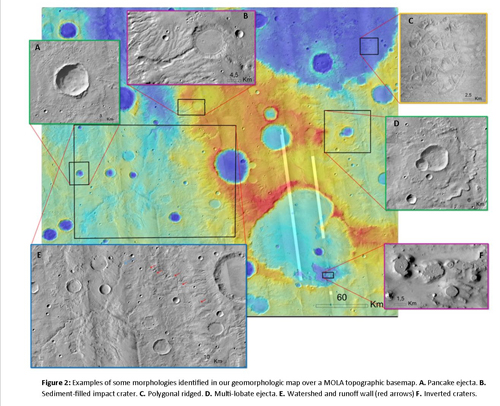
The study area (148.155 km2, Figure 1) is located in the southern equatorial region of Mars, approximately centered at 26.0° S and 6.5° E. Although subjected to extensive surface erosion, this heavily cratered region, selected as a representative section of the densely cratered highlands [1], still shows evident signs of past water erosion in the form of valley networks that regularly dissect the surface. As such, is an ideal area to study the role of water in modifying the surface of the Martian highlands.
The top elevation of the mapped region is located in the central and eastern areas, reaching a maximum elevation of 2,606 meters above the Martian datum (a.m.d.). The points of lower elevation in the area are locally inside impact craters (-678 m a.m.d.). We found two unusually large impact craters. One is at the northeast, about 180 km in diameter, and only its southern half is inside the area. The other is at the southeast, irregularly shaped, and 116 km in diameter. The topography in the mapped region is also defined by two large valley network systems which carve the surface flowing from south to north, and surround the positive relief at each flank.
We have produced a 1:500.000 scale geomorphological map with unprecedented detail, using ArcGIS 10.3 Desktop Software (ESRI) to draw and compiled a combination of a mosaic of hi-resolution CTX images, complemented by available Context Camera (CTX) images for cover gaps [2], a mosaic composed by MOLA and HRSC topography [3], and THEMIS-IR day imagery [4].
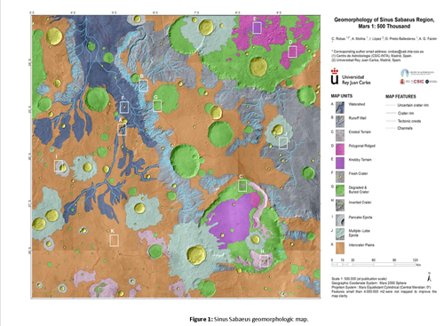
We mapped the main morphological units to contribute to the understanding of the hydrology of
this understudied region of Mars. We mainly focus on describing eleven different morphological units
and four geomorphic features (Figure 2), related to the past presence of water, as both ice and liquid,
to allow us to characterize the past environment and eventually to identify their presence and
persistence.
Among these units we would like to highlight the watershed unit, formed by incisions on the
surface that we interpret as evidence of aqueous activity, in which water came from channels that
flowed by the runoff wall unit. We differentiate a few types of impact craters, highlighting the inverted
crater unit and the sediment-filled impact crater unit, both filled up with sedimentary materials maybe
sourced by paleo-lakes. We differentiate two ejecta units related to liquid and ice water reservoirs;
and a polygonal ridged unit and a knobby terrain unit associated with permafrost environments.
Acknowledgments: This research is a contribution of the Project ”MarsFirstWater”, European
Research Council, Consolidator Grant no. 818602. Authors also thank the Agencia Estatal de
Investigación (AEI) project no. MDM-2017-0737 Unidad de Excelencia ”María de Maeztu”, and Rey
Juan Carlos University.
References: [1] Forsberg-Taylor, et al., (2004). Journal of Geophysical Research: Planets, 109
(E5). [2] Fergason R.L. et al. (2018) Astrogeology PDS Annex, USGS. [3] Dickson J.L. et al. (2018)
49th LPSC, Abstract#2083. [4] Christensen, P. R et al. (2004). Space Science Reviews, 110 (1), 85–
130.
How to cite: Robas, C., Molina, A., López, I., Prieto-Ballesteros, O., and Fairén, A.: The role of water on Sinus Sabaeus region, Mars, Europlanet Science Congress 2020, online, 21 Sep–9 Oct 2020, EPSC2020-967, https://doi.org/10.5194/epsc2020-967, 2020.
A beneficial outcome of ExoMars Rosalind Franklin Rover (ERFR) 1,2 landing site selection process has been the spinout science from detailed studies of parts of Mars that had not previously been examined in detail. Here, we present the geological description of Aram Dorsum3 (Fig. 1), a well-preserved, flat‐topped, branching, ~85 km long and ~ 1 km wide ridge system in western Arabia Terra that was a ‘top 3’ candidate site during ERFR site selection.
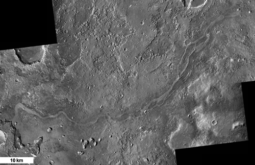
Fig 1. CTX Mosaic Showing Aram Dorsum (sinuous ridge running top right to lower left).
We use morphostratigraphic mapping of the Aram Dorsum ridge and surrounding area, and detailed morphological observations, to propose a consistent working hypothesis for the geological history of the region. Our observations and mapping reveal Aram Dorsum to be the sedimentary deposits of an extensive aggradational fluvial channel belt system, now preserved in positive relief by differential erosion. The existing ridge was once a large river channel belt set in extensive flood plains, many of which are still preserved.
Aram Dorsum is part of a wider set of similar inverted channels found across Arabia Terra4,5, and thus was probably part of a regional fluvial system, demonstrating movement of water and sediment across large distances. Furthermore, several smaller palaeochannel belts feed into the Aram Dorsum ridge from within the local regions, and their setting and network pattern suggest a distributed and local source of water. Aram Dorsum therefore appears to record both regionally and locally distributed sources of water.
Combining mapping with HiRISE6 and CTX7 Digital Elevation Model data reveals that the Aram Dorsum alluvial succession is up to 60 m thick, suggesting a formation time of 105 to 107 years by analogy to Earth8. Correlating our observations with previous regional‐scale mapping9 shows that Aram Dorsum formed in the mid‐Noachian, a result supported by impact crater size frequency distribution measurements.
The Aram Dorsum formation comprises a succession of what are, by analogy with terrestrial fluvial systems, probably coarse‐grained fluvial channel belt sandstones and finer‐grained overbank deposits. The vertical thickness of alluvial succession equates to several cubic kilometres of fluvial sediments in this study region alone. That other inverted channels elsewhere in Arabia Terra4,5,10 are similar in morphology and scale suggest that similar thicknesses and volumes of mid‐Noachian to late‐Noachian fluvial sediments may be extensive and common in the wider region.
Aram Dorsum was an extensive long-lived fluvial system with distributed sources. This suggests that local and regional precipitation (either as rain or as seasonal or repeated snow melt) was the source of water. That Aram Dorsum is one of several similar systems suggests that precipitation was widespread across western Arabia Terra during this period. In contrast, Aram Dorsum's low elevation and distance from the majority of the Valley Networks, argues against the source of water being melting of a distant, high‐altitude, ice sheet, or ice cap11,12. Similarly, the aggradational fluvial depositional setting and the scale of the system do not suggest deposition from multiple short‐lived fluvial flows, as might have occurred due to impact cratering or catastrophic volcanic outgassing temporarily altering the climate12–15. We conclude that Aram Dorsum is one of the oldest fluvial systems described on Mars and indicates climatic conditions that sustained surface river flows on early Mars.
References cited
How to cite: Balme, M., Gupta, S., Davis, J., Fawdon, P., Grindrod, P., Bridges, J., Sefton-Nash, E., and Williams, R.: Aram Dorsum: An Extensive Mid‐Noachian Age Fluvial Depositional System in Arabia Terra, Mars, Europlanet Science Congress 2020, online, 21 Sep–9 Oct 2020, EPSC2020-446, https://doi.org/10.5194/epsc2020-446, 2020.
Melting of ice is physically difficult to achieve under present-day Mars conditions [1,2,3], and the observational evidence for liquid water is ambiguous. The frost point temperature on Mars (~200 K) is far below the melting point of pure ice (273 K). Hence, water ice diffuses into the ambient atmosphere long before it reaches the melting point. Moreover, the total pressure of the atmosphere lies near the triple point pressure, so that ice near 0°C sublimates so rapidly that evaporative cooling exceeds the solar constant [1]. Here, one specific pathway for the formation of liquid water on present-day Mars is quantitatively evaluated: Melting of seasonal water frost in rough terrain [4]. In areas that are seasonally shadowed, water frost accumulates, and when the sun rises again, temperature increases rapidly. A rapid transition from cold to hot will involve little sublimation loss. A suite of quantitative models is used to investigate whether seasonal water frost can melt on present-day Mars.
When the water vapor content of the atmosphere is a non-negligible fraction of the total atmosphere pressure, as will be the case near melting, there is a strong buoyancy force that leads to free turbulent convection and strong evaporative cooling. The classical parametrization of the turbulent flux [1] has been updated based on more recent literature [4].
To obtain surface temperatures, a numerical model is used that includes direct solar irradiance, subsurface conduction, terrain shadowing, terrain irradiance, and sky irradiance. The surface energy balance is integrated over time at steps of 1/50th of a solar day (sol) for several Mars years.
The model site is at a latitude of 30°S and assumes a thermal inertia of 400 Jm-2K-1s-1/2. For a boulder, idealized as a half-sphere that sticks out from the surface, the situation is favorable. Beyond the southern (poleward) end of the boulder, water frost continuously accumulates for hundreds of sols, decimeters of CO2 frost also accumulate [5], and, when evaporative cooling is not considered, peak temperatures are well above the melting point. The location is seasonally shadowed around the winter solstice. Once the sun rises, the CO2 ice begins to sublimate, but the CO2-H2O ice composite cannot warm until all of the CO2 ice has disappeared. The first day of spring without seasonal CO2 frost is known as "crocus date''. After the crocus date, the surface temperature rises from 145 K to 273 K from sunrise until noon.
With evaporative cooling, the surface does not reach the melting point. On the first full sol after the crocus date, the temperature rises to 256 K and 0.1 kg/m2 of frost (a 100 μm thick layer) are lost until it first reaches this temperature. The next day, the peak temperature is 260 K and at this point 0.5 kg/m2 of frost have been cumulatively lost. The evaporative cooling is too strong to allow 273 K to be reached. The Viking 2 Lander observed almost continuous early frost 10-20 μm thick, and later patchy frost probably 100-200 μm thick [6]. More frost may accumulate in well-shadowed alcoves. Hence, the mass lost within a sol or two after the crocus date is within the amount that can be expected to be present.
The thermal model calculations demonstrate that sudden transitions from frost-accumulating conditions to near-melting conditions occur, but ultimately there is not enough energy available to compensate for the evaporative cooling. An energetically favorable situation is the sun rising at the equator at perihelion. In this case, peak temperatures within about 10 K of the melting point within one or two sols of the crocus date are realistic.
Protruding topography in the mid-latitudes creates locations that experience a rapid transition from conditions where water frost accumulates to high solar energy input. Beyond the pole-facing side of a boulder, CO2 and H2O frost can accumulate seasonally, and when the CO2 frost disappears in early spring, the water frost is heated to near melting temperature within one or two sols. The rapid temperature rise occurs on and following the crocus date. Evaporative cooling prevents temperatures from rising to 273 K even at an atmospheric pressure as high as 1000 Pa and even with a sublimation lag of several mm of dust. Overall, melting of pure seasonal water ice is not expected under present-day Mars conditions. Dark water frost (albedo 0.15) can reach peak temperatures within about 10 K of the melting point, and the loss of ice experienced during the warming phase is no larger than the amount of seasonal water frost that can be expected to be present. For bright water frost (albedo 0.4) peak temperatures within about 15 K of the melting point are realistic.
At these temperatures, seasonal water frost can melt on a salt-rich substrate. Hence, crocus melting behind boulders can lead to the formation of brine under present-day Mars conditions. Salts are commonplace on Mars and have a range of eutectic temperatures. The temperatures produced through crocus melting behind boulders would suffice, even at atmospheric pressures below that of the triple point of pure water. The process will repeat periodically as long as the salt is not depleted. Overall, it is realistic that seasonal water frost melts on salt-rich ground. Since the seasonal H2O frost layer is very thin, the total volume of brine produced is small.
Acknowledgments: This material is based upon work supported by NASA through the Habitable Worlds Program.
References: [1] A.P. Ingersoll (1970) Science 168, 972. [2] M.A. Kreslavsky & J.W. Head (2009) Icarus 201, 517. [3] M.H. Hecht (2002) Icarus 156, 373. [4] N. Schorghofer (2020) ApJ 890, 49. [5] K.J. Kossacki & W.J. Markiewicz (2004) Icarus 171, 272. [6] T. Svitek & B. Murray (1990) JGR 95, 1495.
How to cite: Schorghofer, N.: Crocus Melting on Mars, Europlanet Science Congress 2020, online, 21 Sep–9 Oct 2020, EPSC2020-175, https://doi.org/10.5194/epsc2020-175, 2020.
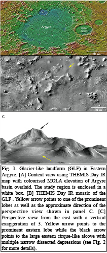
Introduction: Glacier-like forms (GLFs) are a particular class of ice-rich landforms that occupies the mid-latitudes of Mars [e.g., 1–4]. They appear to be concentrated around the 40º–55º latitude range in both hemispheres [3,4]. Here we present results from an ongoing geological investigation of what we interpret to be a debris-covered mountain glacier in the Argyre basin. The glacier system displays 1) multi piedmont-like terminal lobes, 2) gullied cirque-like source regions, 3) flows reaching ~35 km with an elevation drop reaching nearly 2 km from source to terminus, and 4) periglacial modification of surface materials indicative of near-surface ice. A better characterisation of this landform may provide clues regarding the formation and evolution of non-polar ice on Mars, particularly during periods of high obliquity.
Geologic Setting: The glacier is located along the inner eastern rim of Argyre basin (Fig. 1), which suggests that the hosting mountain is an erosional remnant of the basin’s rim materials [e.g., 5]. The mountain has an elevation of ~3250 m and rises ~4250 m above the surrounding terrains to the east, and more than 6000 m above the Argyre floor to the west. It displays a wide mesa-like flat top more than 20 km across along its longest axis with steep (22–30°) sides that have developed into cirque-like alcoves. Two prominent alcoves face NE and NW and their walls are highly dissected by narrow depressions resembling gullies. The mountain displays 3 distinct lobes that appear to flow from the base of the cirques trending NE, NW, and SW, among other minor flows, while a lobate debris apron extends to the SE.
Observations: We created a CTX mosaic for the study region and georeferenced it to an HRSC DTM to extract morphometric information on flow directions and influence of surrounding topography, and complemented this with a morphologic investigation using HiRISE images.
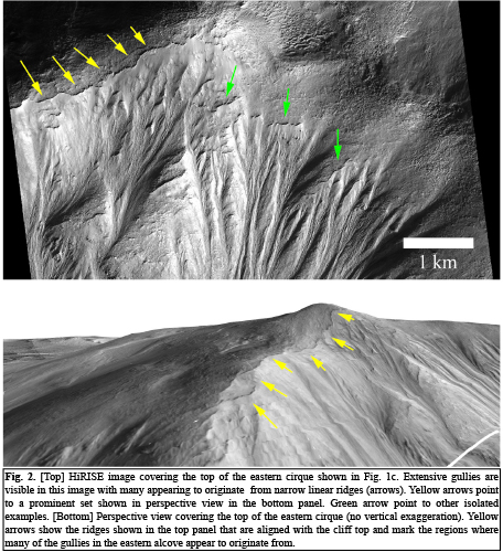
Paleo-accumulation regions: The source region for many of the flows appears to be the central mountain. Near the top, large cirque-like structures are visible that show extensive networks of gullies of variable widths and cross cutting relationships suggesting multiple, and varying, erosion cycles through time. Many of the drainage systems appear to originate from quasi-linear ridges, which are closely aligned with each other at the top of the mound (Fig. 2). We interpret these ridges to be the paleo-boundaries between the drainage systems and past ice-rich deposits at the mountain top, which contributed to the drainage systems.
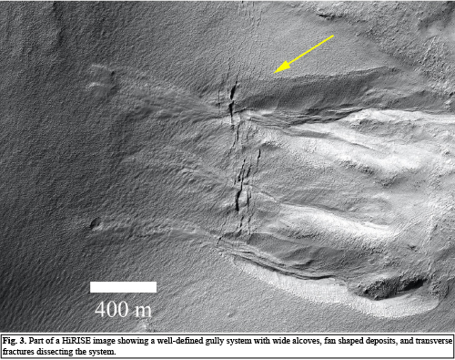
Fractures and gullies: On the western slopes of the central mountain, a number of distinctive gullies show deep alcoves, terminal fan-shaped deposits, and transverse fractures that cut through the gully system (Fig. 3). This type of transverse fractures that are quasi normal to the general slope suggest long-term modification following the gullies formation, which could be a result of periglacial modification, volatile loss, slowly flowing ice, or a combination of these processes.
Surface periglacial modification: High resolution images covering multiple locations in the glacier system show that the surface is pervasively modified showing patterned grounds, which we interpret to be seasonal thermal contraction polygons. In areas of pronounced slopes, surface patterns appear to be additionally aligned with these slopes with fractures that are transverse to the slope direction showing preferential widening. Such locations are likely preferential zones for volatile loss. In certain cases, the fractures widen to create wide troughs (Fig. 4). We plan to present these findings, among others, in the meeting in more detail and discuss their possible implications.
References: [1] Arfstrom, J., and Hartmann, W.K., (2005), Icarus, 174, 321–335. [2] Head. J.W. et al. (2010), EPSL, 294, 306–320. [3] Souness, C. et al. (2012). Icarus, 217, 243–255. [4] Hubbard, B. et al. (2014), Cryosphere, 8, 2047–2061. [5] Dohm, J.M. et al. (2015), Icarus, 253, 66–98.
How to cite: El-Maarry, M. R. and Diot, X.: Geologic Investigation of a Debris-covered Mountain Glacier in Argyre Basin, Mars: Implications for Past Climate and History of Non-Polar Ice, Europlanet Science Congress 2020, online, 21 Sep–9 Oct 2020, EPSC2020-222, https://doi.org/10.5194/epsc2020-222, 2020.
Abstract
We are exploring mass wasting at the scarps of the Martian North Polar Layered Deposits (NPLD) by probing into collapsed ice-fragments using multi-temporal HiRISE images. We apply change detection techniques to the images in areas of steep scarps and then determine sizes and volumes of the ice-fragments using boundary mapping in image pyramids. Our aim is to map the sources of block fall events through time, estimate volumes of displaced material and investigate their seasonality in order to better understand the behavior of the ice scarps and gain insights into their evolution.
1.Introduction
The steep scarps at the boundary of the NPLD have shown evidence of mass wasting in recent decades [1]. In particular, dust avalanches and ice-block falls, are probably related to thermoelastic stresses [2]. Ice-block falls are playing a significant role of active erosion at the north polar scarps of Mars [3,4,5]. Data from the High Resolution Imaging Science Experiment (HiRISE), including multi-temporal images with scales of up to ~0.25m/pixel, make it possible to identify small-scale changes [6]. Fanara et al. (2019) estimated the erosion rate of a scarp by detecting block falls and have found seven areas with similarly fractured scarps [5], from which ice-fragments detach and finally fall as ice-blocks. Figure 1 shows three sets of examples from different scarps, where ice-fragments have been detected in Mars Year 31 and have disappeared in Mars Year 32 (red arrows). The red circle in Figure 1a indicates the ice-block falls from the collapsed ice-fragment. Considering the active erosion during the past decades, we want to investigate the sources of the block falls and map them through time.
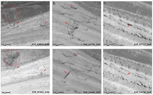
Figure 1. Three sets of images from different scarps between Mars Year 31 (first row) and Mars Year 32 (second row) show collapsed ice-fragments (red arrows). The red circle shows a resulting block fall event.
2.Method
Based on two ortho-rectified HiRISE images processed by Ames Stereo Pipeline (ASP) at different times, we detect the collapsed ice-fragments’ areas. We focus on images taken during the summer of Mars because the covering CO2 ice sublimates in spring and then the scarps will show distinct textures in summer. Before the ice-fragments collapse, they have shadows due to the solar incidence. While after the ice-fragments fall down, the original shadows disappear, allowing us to detect the active erosion.
We often find that for ortho-rectified images, co-registration must be refined. For this, we use image matching techniques. First, we use the normalized cross-correlation to find the approximate corresponding position of two images. Then, we divide both images into multiple tiles to avoid geometric deviations in different areas over the entire image. Regarding regional changes due to collapsed ice-fragments, intensity-based matching methods are sensitive, while optimized feature matching can work well. So, we use feature-based matching method combined with affine transform on all tiles to align them. In order to reduce radiometric differences caused by illumination, atmosphere and other conditions, we apply Wallis filter for radiometric normalization. Lastly, we obtain the difference image by subtraction and set a threshold to get the binary difference image, which shows the changed area.
On the difference image, the obvious discrepancy between the two images are the shadow areas. However, it is not always easy to distinguish the complete boundaries of the ice-fragments. So we intend to detect fuzzy edges via image pyramids and contrast enhancement in order to calculate the fragments’ areas.
The height of the ice-fragments are also critical for calculating the volume of the material loss. The vertical precision of HiRISE DEM is about tens of centimeters [6]. However, most of the fragments’ heights are ~1m, thus it is hard to determine elevation differences through DEMs. Therefore, we will combine the solar incidence angle with the shadow length of the ice-fragments to calculate their height.
3.Discussion
Our research focuses on the investigation of the source areas of block falls at the NPLD. The change detection method results in maps of the areas of active erosion through time. This way we derive important temporal and spatial constraints as well as volume estimations for the ongoing block fall activity. Ultimately we want to analyze the scarp activity based on the correlation of our results with seasonal and morphological parameters to help understand the ice behavior and the evolution of the NPLD scarps.
Acknowledgements
The first author thanks China Scholarship Council (CSC) for the financial support to study in Germany.
References
[1] Russell, P. S., et al. 5th ICMPSE. Vol. 1623. 2011.
[2] Byrne, S., et al. EPSC. Vol. 11. 2017.
[3] Herkenhoff, K. E., et al. Science. 317.5845 (2007): 1711-1715
[4] Russell, P. S., et al. 8th Intern. Conf. on Mars. Vol. 1791. 2014.
[5] Fanara, L., et al. 113434. 2019.
[6] McEwen, Alfred S., et al. JGR. 112. E5. 2007.
How to cite: Su, S., Fanara, L., Zhang, X., Gwinner, K., Hauber, E., and Oberst, J.: Sources and characteristics of block falls at the Martian north polar scarps, Europlanet Science Congress 2020, online, 21 Sep–9 Oct 2020, EPSC2020-267, https://doi.org/10.5194/epsc2020-267, 2020.
Abstract
This work focuses on the study of the characteristics and possible origin of distinct positive topographic landforms located in Scandia Cavi and Olympia Undae [1]. These are two regions close to the northern polar cap of Mars and which are of special interest because of the potential joint presence of volcanism, glacial processes and gypsum deposits which could be related to the past presence of liquid water there. Such processes can cast light on the geological evolution of the area.
We use images from Mars Express and Mars Reconnaissance Orbiter, as well as MOLA topographic profiles from Mars Global Surveyor to investigate 201 small and medium-size landforms in these two regions. These landforms have a priori similar characteristics, such as similar sizes and forms, but their origin might not be the same. A detailed analysis of images and morphometric parameters has allowed their classification into 6 groups, which are the so-called cratered cones, impact craters, ambiguous craters, simple and peaked domes, and irregular structures.
Different possible origins for these landforms are discussed such as impact, aeolian, glacial and volcanic processes. The possible implications for relationships between an available volcanic heat source nearby water ice and gypsum deposits make the area particularly interesting toward further constraining the region’s geology.
References
[1] Sánchez-Bayton et al., Morphological analyses of small and medium size landforms in Scandia Cavi and Olympia Undae, North Polar Region of Mars, under review at Journal of Geophysical Research: Planets
How to cite: Sánchez-Bayton, M., Treguier, E., Herraiz, M., Martin, P., Kereszturi, A., and Sánchez-Cano, B.: Morphological study of landforms in the Northern Polar Region of Mars, Europlanet Science Congress 2020, online, 21 Sep–9 Oct 2020, EPSC2020-366, https://doi.org/10.5194/epsc2020-366, 2020.
Abstract
We propose the co-registration of local laser profile segments to high resolution Digital Terrain Models (DTMs) as an approach for obtaining seasonal CO2 ice cover height variations on Mars. The co-registration is parameterized in instantaneous MOLA pointing angles involving a rigorous laser altimeter geolocation model. Thereby, the height bias of the MOLA footprint produced by the pointing bias could be compensated through an iterative process. The feasibility and advantages of this method are tested in an example region. The ultimate goal is to apply this method to Mars Orbiter Laser Altimeter (MOLA), SHAllow RADar (SHARAD) radar altimetry and high-resolution stereoscopic DTMs to generate long-term seasonal height change time series at the Martian poles with high spatial and temporal resolution.
1 Introduction
The dynamic growth and retreat of polar CO2 frost at the Martian poles has always been one of the focuses of planetary scientists [1, 2, 3]. Accurate measurements of seasonal and long-term elevation and volume changes can serve as important constraints in Mars climate models, help tap into the density evolution of the CO2 snow once combined with gravity measurements, and constrain the degree of stability of the polar deposits. The commonly-used approach to this problem is the cross-over analysis of the laser altimetry profiles, but this method may suffer from significant interpolation errors when spacing between footprints is large, also residual pointing, timing and orbit error may translate into lateral shifts of the laser profiles and further undermine the results. Here, we propose and validate the local co-registration between laser profile segments and high resolution DTMs from stereo pairs as a solution to these limitations.
2 Data
2.1 MOLA records
The MOLA Precision Experimental Data Record (PEDR) dataset features a total of 8505 profiles, acquired in the mapping and extended phases of Mars Global Surveyor (MGS) from February, 1999 to May, 2001, which spanned approximately a full Martian year [1]. The PEDR dataset was processed using MGS orbit trajectory model and a Mars rotational model by GSFC dating back to 2003. Therefore, we have incorporated a refined orbit model from [4] and IAU2015 Mars rotational model [5] in the MOLA geolocation reprocessing. Meanwhile, to account for the special relativity effect, the pointing aberration correction has also been taken care of in the reprocessing [6].
2.2 HRSC DTMs
The High Resolution Stereo Camera (HRSC) is a pushbroom camera onboard the European Space Agency (ESA) spacecraft Mars Express. A total of 34 HRSC DTM tiles are adopted which feature a grid size of 50 m and covers the majority of the Martian South Pole [7].
3 Methods
First, the reprocessed MOLA profiles are self-registered to each other to form a coherent reference in the Martian South Pole [8, 9]. Subsequently, individual HRSC DTM tiles have been aligned to the MOLA reference data and mosaiced to a self-consistent reference for the co-registration. The co-registration of the reprocessed MOLA profiles to the aligned HRSC DTM mosaic is setup by compensating for two alignment angles of the boresight and height which incorporates an analytical laser altimeter geolocation model. The benefit is that the height offset induced by bias in pointing can be simultaneously compensated during the iterative co-registration process. The height differences with respect to the DTM mosaic at either footprint, cross-overs, or pseudo cross-overs are assigned as the height corrections from the local co-registration process using segmented profiles centered at these feature points. Here, pseudo cross-overs are DTM-based and formed by two track segments that do not have to actually intersect, substantially increasing the available number of cross-overs [10]. Then, CO2 height change time series are obtained by median-binning those temporal height differences with the uncertainty quantified by scaled median absolute deviation. To get rid of a temporal systematic error, the acquired temporal trend is subtracted from the one at 60°S annulus which features unchanging topography.
4 Results
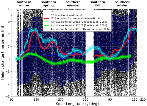
Figure 1: Results using height differences at footprints before the adoption of the local co-registration procedure (“F_LC”, red line, bottom) and comparison to previous literature (lime and aqua lines).
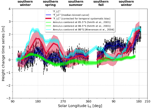
Figure 2: Results using height differences at footprints after the adoption of the local co-registration procedure (“F_LC”, red line, bottom) and comparison to previous literature (lime and aqua lines).
A test has been carried out at an example region situated right on the residual ice cap where largest peak-to-peak height variation would be expected. The uncertainty of the derived height change time series using height differences at footprints decreased from ~2 m to ~0.5 m after the adoption of the local co-registration procedure, roughly a fourfold enhancement (Figures 1 and 2). The maximum height fluctuation is estimated at ~2.5 m which is similar to that of Aharonson et al. (2004) [2]. The suspicious off-season accumulation pointed out by previous results using MOLA has not been resolved. While a sharp pit-shaped feature of ~1 m depth centered at solar longitude 210° is observed. Similar results have been obtained using height differences at cross-overs and pseudo cross-overs. As a byproduct of the co-registration process, MOLA alignment angles have also been examined to follow some specific temporal patterns.
5 Summary
We show the feasibility and merits of the local co-registration strategy in the application of retrieving height changes at either footprints, cross-overs, or pseudo cross-overs. As for the next step, we will put the SHARAD radar altimetry and reflectometry into test [11]. Combined with the MOLA laser altimetry, long-term CO2 height change time series spanning two decades could possibly be retrieved. Apart from height change mapping, the proposed method could also be readily adapted to the tidal Love number measuring, orbit refinement with so called “direct altimetry” [12] and others.
Acknowledgements
This work was supported by a research grant from Helmholtz Association and German Aerospace Center (DLR). We acknowledge the work by the MOLA and HRSC instrument and science teams.
References
[1] Smith et al.,Science, 2001, 294, 2141-2146.
[2] Aharonson et al., JGRPlanets, 2004, 109(E5).
[3] Genova, ActaAstronaut., 2020, 166, 317-329.
[4] Konopliv et al., Icarus, 2006, 182, 23-50.
[5] Konopliv et al., Icarus, 2016, 274, 253-260.
[6] Xiao et al., Submitted to JoG.
[7] Putri et al., PSS, 2019, 174, 43-55.
[8] Stark et al., EPSC2018, Contrib. No. 890.
[9] Stark et al., GRL, 2015, 429, 7881-7889.
[10] Barker et al., Icarus, 2016, 273, 346-355.
[11] Steinbrügge et al., LPSC2019, LPI Contrib. No. 2132.
[12] Goossens et al., Icarus, 2020, 336, 113454.
How to cite: Xiao, H., Stark, A., Steinbrügge, G., Neumann, G., and Oberst, J.: Co-registration of MOLA profiles to HRSC DTMs for mapping local seasonal ice cover height variations at the Martian poles, Europlanet Science Congress 2020, online, 21 Sep–9 Oct 2020, EPSC2020-181, https://doi.org/10.5194/epsc2020-181, 2020.
1. Introduction. Mars is currently characterized by a hypothermal, hyperarid climate that is thought to have persisted throughout the Amazonian [1]. The distribution of water ice on Mars has changed over time due to periodic variations in spin axis obliquity [2]. During periods of relatively higher obliquity than present, water ice is mobilized from the poles and deposited as snow and ice in the mid-latitudes, producing cold-based glacial landforms (Fig. 1A-B) [3-6].
Geologic evidence suggests that the ambient climate in the Noachian was significantly different. Fluvial and lacustrine features have been interpreted to indicate the presence of a warm and wet climate [7-8]. However, global climate models predict Noachian temperatures well below those required to sustain liquid water at the surface [9-10]. These models also predict that the distribution of water ice will mostly be controlled by altitude rather than latitude. Supporting geomorphic evidence for this hypothesis has been elusive because glaciation in such an environment is predicted to be cold-based and, as in the Amazonian, melting is limited to top-down (supraglacial) sources [11]. We can search for characteristic cold-based glacial morphologies preserved in high-altitude terrains in order to better assess the character of potential cold-based glacial processes in the Noachian [12].
2. Geology of Crater B. We report on the geology of a 54-km Noachian-aged crater in the southern highlands that displays evidence for cold-based glaciation. The crater is located in ~800 km northwest of the Hellas basin rim in Terra Sabaea. In a study of eroded crater floors in the same region, Irwin et al. [13] noted that the interior of this crater, which they designated “B,” contains a characteristic dark-over-light stratigraphy that is repeated in many other nearby craters. Inverted ridges are preserved in the more erodible dark unit and are likely fluvial in origin.
On the basis of this previous work, we mapped the interior of this crater in detail using CTX and HiRISE visible images. These data reveal an ensemble of additional features (Fig. 1C, 2) not previously described in Noachian-aged craters that indicate a history of cold-based glaciation and top-down melting.
A series of arcuate, upslope-facing scarps occurs near the base of the crater wall; each segment typically corresponds to a single upslope alcove. These scarps are positive relief features consistent with the deposition of moraines originating from cold-based glaciers flowing downslope from the alcoves. The heads of the inverted fluvial ridges closely follow the orientation of the scarps as they bend around the alcoves. A thin debris apron consistent with proglacial sedimentation occurs along the base of the crater wall, superposing the scarps and inverted ridge heads. We derive a lower limit crater age date of ~3.5 Ga, or Late Noachian–Early Hesperian (LN–EH), for the ensemble of cold-based glacial features in the crater based upon the superposition of the debris apron over the other units.
The largest system of inverted fluvial ridges extends 45 km circumferentially around the northeastern crater floor and terminates near the modern topographic low point of the crater. A second, smaller system of inverted ridges originates from the southern crater wall and terminates at the margin of a smaller deposit that sits ~30 m higher than the first basin.
3. Discussion and Conclusions. We interpret the alcove-scarp-ridge system (Fig. 1C) as the result of top-down melting of a cold-based crater wall glacier, leading to proglacial outwash in the form of fluvial channels that transported glacially derived sediment into multiple low-lying basins in the crater floor. The fine-grained channel effluent was likely removed by eolian erosion, which could also have modified the paleotopographic surface such that a slight difference exists between the current elevation of the two depositional basins. Outcrops of a lighter-toned indurated substrate are coincident with the lowest and most extensively deflated areas of the crater floor.
The endorheic crater B basin, with completely internal drainage, lies in contrast to the similarly-aged open- and closed-basin lakes on Mars [14-15]. The lack of significant exterior drainage into crater B argues against an origin for the inverted ridges as the depositional remnants of fluvial valley networks derived from areally distributed rainfall and runoff. Likewise, groundwater sapping is unlikely to produce the dense, high stream-order ridges we observe.
We hypothesize that a brief period of atmospheric warming caused top-down melting of cold-based crater wall glaciers during the transition from Noachian climate conditions to conditions typical of the later Hesperian and Amazonian. Recognition and documentation of these features provides specific criteria to search for other examples of past glaciation in the southern highlands in order to further test hypotheses of Mars climate evolution.
References. [1] Carr M.H., Head J.W. (2010) EPSL 294; [2] Laskar J. et al. (2004) Icarus 170; [3] Berman D.C. et al. (2005) Icarus 178; [4] Jawin E.R. et al. (2018) Icarus 309; [5] Berman D.C. et al. (2009) Icarus 200; [6] Fassett C.I. et al. (2010) Icarus 208; [7] Craddock R.A., Howard A.D. (2002) JGR 107; [8] Ramirez R.M., Craddock R.A. (2018) Nature Geo. 11; [9] Forget F. et al. (2013) Icarus 222; [10] Wordsworth R. et al. (2013) Icarus 222; [11] Fastook J.L., Head J.W. (2015) PSS 106; [12] Marchant D.R., Head J.W. (2007) Icarus 192; [13] Irwin R.P. et al. (2018) JGR 123; [14] Fassett C.I., Head J.W. (2008) Icarus 198; [15] Goudge T.A. et al. (2015) Icarus 260.
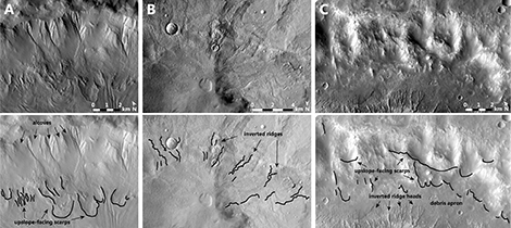
Fig. 1. (A) Amazonian cold-based glacial morphologies in an unnamed crater in Terra Sirenum. Moraine scarps mark former locations of glacial lobes. (B) Amazonian glaciofluvial valleys in the crater Greg have been inverted into ridges on the crater floor. (C) Degraded remnants of lobes and scarps are still preserved in crater B. The scarps are closely associated with the position of the debris apron and inverted ridge heads.
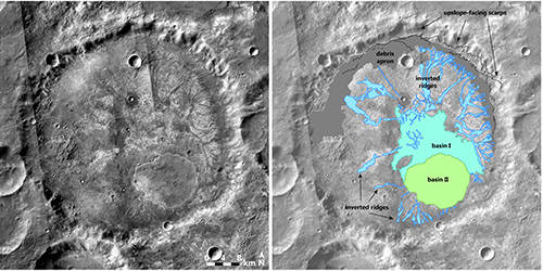
Fig. 2. CTX mosaic of crater B and sketch map overlay showing the major geologic features within crater B. Inverted tributary ridges begin near the crater wall base in association with upslope-facing scarps and debris apron and terminate in two depositional basins.
How to cite: Boatwright, B. and Head, J.: Noachian Crater Modification on Mars: Evidence for Cold-Based Crater Wall Glaciation and Endorheic Basin Formation, Europlanet Science Congress 2020, online, 21 Sep–9 Oct 2020, EPSC2020-976, https://doi.org/10.5194/epsc2020-976, 2020.
Introduction: Hale Crater is located on the north-eastern rim of Argyre Basin (35.7°S, 323.6°E and has been dated to 1 Ga (Early to Middle Amazonian; Jones et al., 2011). This complex crater is elliptical (125 km across compared to 150 km wide), which can be explained by an oblique trajectory of an impactor from the South-East. This hypothesis is supported by the asymmetrical expression of its central peak and ejecta blanket (Jones et al., 2011). Its ejecta and interior show evidence for an ice-rich composition of the target surface: the ejecta are lobate and bear channels, and the interior is pervasively pitted with alluvial fans (El-Maarry et al., 2013; Jones et al., 2011; Tornabene et al., 2012). The ejecta also hosts conical mounds. Here we test the hypothesis that these mounds are “molards”. Molards are conical mounds of debris that are formed by the loss of cementing ice from frozen blocks that have been transported in landslides in periglacial environments on Earth (Morino et al., 2019). We suggest that the conical mounds in the Hale ejecta result from the degradation of blocks of ice-cemented ground transported by the ejecta flows.

Approach: We have performed a regional and local analysis of the geomorphological setting, morphometry and morphometrics of the conical mounds in the Hale Crater ejecta. We focussed on a study area (240x180 km) in the South-East part of the Hale Crater ejecta (-36.0° – -39.0°N, 36.0° – 31.0°W), where the majority of mounds are found. The regional map was based on 25 m/pix images from the High Resolution Stereo Camera (HRSC on Mars Express). The associated Digital Elevation Models (DEMs) have a spatial resolution of 125-150 m/pix. The HRSC images were used as a base for georeferencing 25 Context Camera images at 6 m/pix (CTX on Mars Reconnaissance Orbiter). Using these data, we refined the Jones et al. (2011) map of the ejecta deposits and channels. We mapped all craters with sharp rims that were filled with the ejecta materials, in order to estimate the ejecta thickness by comparing the measured (filled) depth of the crater with the expected depth using the theoretical depth-to-diameter relationship.
High Resolution Science Imaging Experiment (HiRISE on Mars Reconnaissance Orbiter) data at 25-50 cm/pix cover limited zones, and we used two stereo-generated elevation models to perform detailed morphometric study of the mounds. We used closed 1 m contour lines to define the outer boundary of individual mounds. From this polygon, we calculated the mound diameter and the maximum elevation pixel, and thus the cone-height. We calculated flank slopes using profiles connecting the highest point of the cone to this outer-boundary. In the analysis presented here, we have used two terrestrial analogues, those in northern Iceland already presented in Morino et al. (2019) and Mount Meager in Canada (Roberti et al., 2017).

Results: The conical mounds in the Hale Crater ejecta are restricted to the inner ejecta, which we have found to be on average 65 m in thickness (Fig. 1). The mounds are concentrated around the channels formed in the inner ejecta and towards its outermost limit (Figs. 1,2). A lower frequency of superposed hundred-metre craters on this part of the ejecta suggests that auto-secondaries were not preserved as this ejecta remained fluid for a prolonged time after the impact. We have found an intimate association between mounds and channels, lobate margins, polygonal ridge patterns and pitted surface of the ejecta – all pointing to a water-rich debris or mud flow. Our comparisons to the Mount Meager debris avalanche support this assertion, where channels, lobes and mounds are also found in a similar spatial arrangement (Fig. 3).

We analysed the morphometrics of 2175 conical mounds in the Hale ejecta, finding diameters between 4 and 238 m (median 26-38 m) and heights between 1 and 53 m (median 5-7 m). Flank slopes ranged from 2 to 42° (median 13-22°; Fig. 4). Compared to a limited sample of 40 molards in Iceland, the conical mounds in the Hale ejecta are larger in spatial scale by one order of magnitude, with Icelandic molards being only up to 22 m in diameter, but usually only a few metres. As the scale of the molards on Earth is thought to scale with the size of the initial ice-cemented block, this result can be explained by blocks being initially several tens of metres to perhaps 100 m in size in the Hale ejecta (consistent with the 65 m average ejecta thickness). The conical mounds in the Hale ejecta have slopes at the lower end of those expressed by Icelandic molards, whose median is 16-35° (Fig. 2), which could be attributed to their extended exposure at the surface causing a decline in the flank slopes. Further work includes comparing to a larger sample of terrestrial molards of varying ages in Greenland and Canada, where we will particularly focus on the range of shapes expressed by molards.

Conclusions:
- We find that the morphology and setting of the conical mounds within Hale Crater ejecta are consistent with the formation pathway of molards on Earth, i.e. they result from blocks of ice-cemented ground that were thrown out in the impact and transported by the ejecta flows, and that degraded to cones of debris on loss of the interstitial ice.
- Comparison with terrestrial analogues reveals important geomorphological similarities between the ejecta flows of Hale and debris avalanches in periglacial environments on Earth, where substantial quantities of water are involved.
References:
El-Maarry, et al. 2013. https://doi.org/10.1016/j.icarus.2013.07.014
Jones, et al. 2011. Icarus 211, 259–272. https://doi.org/10.1016/j.icarus.2010.10.014
Morino, et al. 2019. EPSL 516, 136–147. https://doi.org/10.1016/j.epsl.2019.03.040
Roberti, et al. 2017. Geosphere 13, 369–390. https://doi.org/10.1130/GES01389.1
Tornabene, et al. 2012. Icarus 220, 348–368. https://doi.org/10.1016/j.icarus.2012.05.022
How to cite: Conway, S., Peignaux, C., Morino, C., Philippe, M., Collins-May, J., Butcher, F., and Roberti, G.: Evidence for ice in the ejecta flows of Hale Crater, Mars, Europlanet Science Congress 2020, online, 21 Sep–9 Oct 2020, EPSC2020-347, https://doi.org/10.5194/epsc2020-347, 2020.
Introduction: Gale crater preserves a 5 km thick sequence of stratified rocks, the lower-most section of which exhibits orbital spectra signatures of clay minerals transitioning up to sulfates over several hundred meters of stratigraphy [1,2]. Understanding the reason for this wet-to-dry change in the mineralogical signature is one of the primary objectives of the Curiosity rover exploration. The rover is currently positioned at the toe of the Layered Sulfate unit (LSu) exposed over a thousand meters in elevation and characterized from orbit by its general-layered texture and spectral signatures of monohydrated and polyhydrated Mg-sulfates [1–4].
Here we reconcile orbital data with new in situ analyses using MastCam and the Remote Micro-Imager (RMI) of the ChemCam instrument to provide an updated documentation of the LSu stratal components at large outcrop scales and at the highest available resolution. We then propose a provisional model for the depositional systems and their evolution in the sulfate unit, hypothesized to reflect overall diminishing availability of liquid water.
Dataset and Methods: The ChemCam RMI can perform long-distance image acquisitions, i.e. several kilometers away, with discernable features between 4-10 cm at 1 km, and 0.2-0.5 m at 5 km in the best focus conditions [5,6]. Beyond 5 kilometers the spatial resolution of HiRISE orbital images is better than that of the RMI, yet both still complement each other by offering orthogonal viewing angles. Usually a series of individual RMI is acquired, forming a mosaic of the target, which are first processed, including dark and flat field correction, then stitched, denoised and slightly sharpened to highlight small-scale contrasts [7].
Using the Visibility Tool of ArcGIS, the RMI mosaics were geolocated within a digital elevation model (DEM) as projected view sheds to enable accurate positioning of the outcrops observed on the RMI into the stratigraphic column (Figure 1).
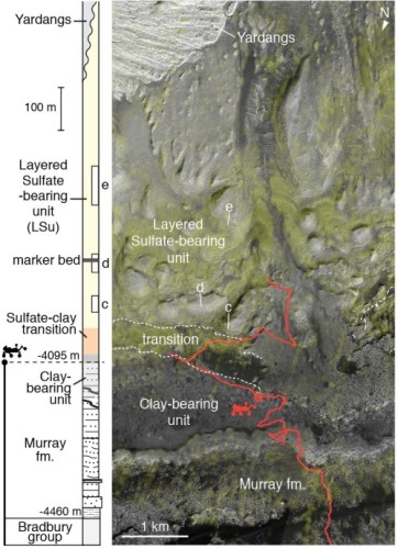
Figure 1: Stratigraphic context and close-up map of Mt Sharp with layered sulfate-bearing unit to be explored by the Curiosity rover. The column represents units elevation (left) along with intervals covered by RMI (Figure 2). Close-up map uses HiRISE MSL basemap overlaid with CRISM S-index in shaded yellow (right). Elevation contours on the sulfate-clay transition (dashed white) are shown with rover path (red).
Large-scale eolian crossbedding: Structures characteristic of large-scale, trough and planar crossbedding are observed in the lower section of the LSu, with large sets bounded by a variety of erosive surfaces (Figure 2c,f). Such cross-bedding forming 5 to 8 meters thick bedsets is most likely diagnostic of aeolian dunes due to its large scale [8]. Overall, no clear tabular crossbedding associated with sand sheet strata has been identified, and structures correspond instead to trough crossbedding as could be formed by superimposed dunes migrating in different directions.
The marker bed as a major deflationary surface: The marker bed is a regionally extensive, thin, smooth, dark-toned layer distinguishable from orbit for 10s of km at a similar elevation around Mt Sharp [2]. Curiosity now observes it in cross-section at higher resolution and reveals a variably prominent, few meter thick, resistant lip which crosscuts underlying strata (Figure 2d,g). The heterogeneous texture includes patches of planar bedded deposits similar to underlying strata and lens-shaped zones of disrupted or rubbly lithologies. Based on geometric and textural evidence, we hypothesize that the marker bed represents a super bounding surface, a type of erosional surface common to terrestrial eolian sequences and corresponding to a break in dunes development [9].
A Fluvial Depositional system in the upper LSu: Above the marker bed, the layering forms decameter thick beds ending with stratal bifurcations, interruptions, or wedgings. Three types of facies can be distinguished: (i) resistant, variably massive bodies; (ii) heterolithic facies with interbedded recessive and resistant elements; (iii) recessive, variably-toned facies. So far in outcrops observed in situ along the Curiosity rover traverse, resistant features of similar scale range from conglomeratic to fine-sandstone lithofacies, whereas recessive intervals are composed of mudstones [10]. We hypothesize that the LSu follows this connection, and propose in our model that the textures could represent a fluvial facies tract, with channel, bank, levee and floodplain deposits (Figure 2e,h).
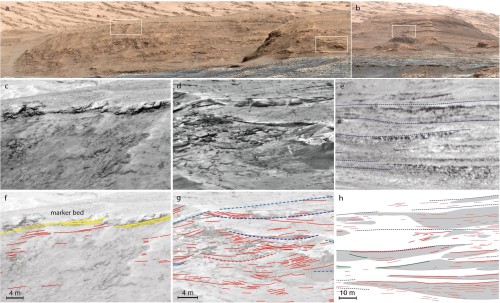
Figure 2: MastCam mosaic of buttes with RMI observations (a: mcam12635; b: mcam06060). RMI mosaic close-ups on sedimentary structures (c-e) and overlayed with tracings (f-h). Modeled structures include: eolian trough crossbedding (f) with bounding surfaces (dashed blue) and sets of cross-strata (red); unconformable boundary at the marker bed (g) with disrupted or rubbly lithologies representing possible lag deposits (shaded yellow) and surrounding strata (red); Fluvial depositional system (h) in the decameter thick layering (dashed lines) with channelized and wedged erosion resistant sandstone bodies (shaded gray) and stratification (red).
Discussion: These observations in the distance, both from orbit and the from the rover, indicate an evolution of depositional environments with fluctuations between wetter and dryer climate at the scale of hundreds of meters in the stratigraphy. Future ground investigation by the Curiosity rover will test and refine the model in these key stratigraphic intervals.
References: [1] Fraeman A. A. et al. (2016) J. Geophys. Res. Planets 121, 1713–1736. [2] Milliken R. E. et al. (2010) Geophys. Res. Lett. 37, L04201. [3] Powell K. E. et al. (2019) LPSC, p. 1455. [4] LeDeit L. et al. (2018) LPSC, p. 1437. [5] Langevin Y. et al. (2013) LPSC, p. 1227. [6] Herkenhoff K. E. et al. (2018) LPSC, p. 2155. [7] Le Mouélic S. et al. (2019) LPSC, p. 2132. [8] Bradley R. W. and Venditti J. G. (2017) Earth-Sci. Rev. 165, 356–376. [9] Kocurek G. (1988) Sediment. Geol. 56, 193–206. [10] Edgar L. A. et al. (2018) Sedimentology 65, 96–122.
How to cite: Rapin, W., Dromart, G., Rubin, D., Le Deit, L., Mangold, N., Fox, V., Gasnault, O., Herkenhoff, K., Le Mouélic, S., Dickson, J. L., Ehlmann, B. L., Maurice, S., Wiens, R. C., and Edgar, L. A.: Predicting changes in depositional environments up Mount Sharp stratigraphy, Europlanet Science Congress 2020, online, 21 Sep–9 Oct 2020, EPSC2020-757, https://doi.org/10.5194/epsc2020-757, 2020.
Introduction: The Glen Torridon (GT) region in Gale crater, has been explored using the Mars Science Laboratory rover, Curiosity, since January 2019 (~Sol 2300) to document clay-bearing rocks initially detected via orbiter data [1]. The rocks are part of the Murray formation, with lower GT consisting of the Jura member mudstones generally associated with a lacustrine deposition [2] overlain by laminated and cross-bedded fine-grained sandstones of the Knockfarril Hill (KfH) member. The latter hint at a sharp change in depositional environment that is critical to investigate [2]. To that extent, we use high-resolution photogrammetric micro-Digital Outcrop Models (DOM) to characterize centimeter-scale sedimentary structures in the KfH member to shed light on their implications in terms of depositional settings and dynamics.
Micro-Digital Outcrop Models (DOM) production using Structure-from-Motion photogrammetry: The MArs Hand Lens Imager (MAHLI) instrument is a color micro-imager on the rover’s robotic arm, able to distinguish coarse silt at a distance of ~2 to 4 cm [3]. MAHLI provides close-up perspectives on rock outcrops and individual targets, notably to assess grain size distribution and sub-mm- to cm-scale sedimentary structures. MAHLI photo mosaics of rock faces typically have sufficient overlapping frames to apply Structure-from-Motion photogrammetry to create 3D micro-DOMs (e.g. [4]). These high-resolution, accurate 3D representations can help us distinguishing sedimentary versus deformational structures from erosional features. Micro-DOMs also enable observation of the outcrop from varying points of view to characterize 3D structures and their lateral/vertical variations. This is especially important in the KfH member due to the very fine-grained nature of the observed sandstones, with cm-scale variations in the sedimentary architecture potentially indicative of rapid shifts in laterally evolving depositional settings. Understanding the nature of the rocks at this scale is also helpful to interpret the chemistry data obtained by the ChemCam instrument from the submillimeter scale (one measurement point) to the centimeter scale (between the points).
Characterization of 3D centimeter-scale sedimentary structures: Here, we focus on three outcrops that exhibit key characteristics of the KfH member of the Murray formation: Morningside (Fig. 1), Stack_of_Glencoul (Fig. 2) and Strathdon (Fig. 3).
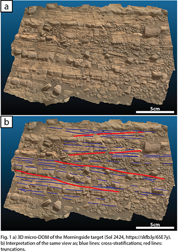
Morningside (Sol 2424, Fig. 1a) is part of an outcrop called Woodland Bay. It exposes a ~45 by ~25 cm patch of fine-grained sandstone that, we think, interfingers with surrounding Jura member mudstones. Morningside exhibits a conspicuous alternation of finely-laminated (mm-scale) and more massive cm-scale beds of fine sandstones. Both the beds and their inner laminations display cross-stratifications with varying directions of propagation (blue lines, Fig. 1b), separated by truncation surfaces (red lines, Fig. 1b). Interestingly, the more massive beds do not appear to result from a potential grading but are rather due to differential resistance to erosion. These structures indicate deposition under moderate but sustained fluvial hydrodynamical flow rather than a quiet lacustrine setting.
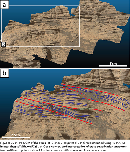
Stack_of_Glencoul (Sol 2444, Fig. 2a) is part of the Teal Ridge outcrop. It displays mm-scale laminations (blue lines, Fig. 2b) arranged in at least four sets of low angle (<15°) cm-scale cross-stratifications, separated by sharp truncation surfaces (red lines, Fig. 2b). These truncations and multiple/alternating directions of propagation in 3D (Fig. 2b) suggest deposition in a dynamic setting such as a fluvial environment. We also observe traces of a complex post-depositional history as indicated by a network of diagenetic veins (some cross-cutting the laminations, others occurring between layers, Fig. 2), identified by ChemCam as calcium sulfate veins (similar to those identified throughout the Murray formation; [5]).
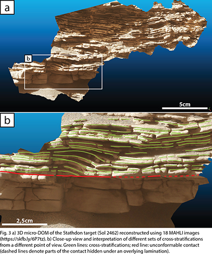
Strathdon (Sol 2462, Fig. 3a) shows sub-cm-scale undulating laminations, highlighted by differential erosion of the outcrop. While these undulations could be ripple marks, burial can also create similar structures [e.g. 6]. Nevertheless, these laminations are characterized by cm-scale cross-stratifications with varying directions of propagation (green lines, Fig. 3b), suggesting an energetic fluvial setting during deposition. In the lower part of the outcrop, undulated laminations are unconformably lying on a more massive bed (red line, Fig. 3b). This contact hints at potentially rapid fluctuations of the hydrodynamical regime between quieter and more energetic settings. Similar to the Stack_of_Glencoul target, Strathdon also displays a network of calcium sulfate veins.
Summary and future work: The production of high-resolution 3D micro-DOMs of centimeter-scale sedimentary structures based on MAHLI images proves to be useful to accurately identify and characterize these structures at a fine scale in the GT region. This is particularly important to assess the rapid lateral and vertical variations of the depositional setting as recorded in the Knockfarril Hill member of the Murray formation. Indeed, the cross-stratifications observed here within the fine sandstones of these outcrops indicate a progressive shift from quiet lacustrine environments of the underlying Jura member, towards a more dynamic fluviatile depositional setting.
These changes (through time and space) might have critical implications regarding the deposition and/or in situ formation of the clay-bearing rocks that are characteristic of the GT region. The documentation of the associated local geochemistry (notably in alkali elements), as documented by the ChemCam instrument, will be integrated in further work to assess whether the geochemical record varies in line with the sedimentary record.
Acknowledgments: EU H2020 PlanMap project.
References: [1] Milliken, R.E. et al. (2010) Geophys Res Lett, 3, L04201. [2] Fedo, C.M. et al. (2020) LPSC abstract #2345. [3] Edgett, K.S. et al. (2015) MSL MAHLI Technical Report 0001, Version 2. [4] Caravaca, G. et al. (2020) Planet Space Sci, 182, 104808. [5] L’Haridon, J. et al. (2018) Icarus, 311, 69-86. [6] Alexander, J. (1987) Geol. Soc. SP, 29, 315-324
How to cite: Caravaca, G., Mangold, N., Le Deit, L., Le Mouélic, S., Dehouck, E., Gasnault, O., Edgett, K. S., Rivera-Hernández, F., Fedo, C. M., and Wiens, R. C.: Using 3D reconstructions of centimeter-scale sedimentary structures to document changes in the depositional settings of Glen Torridon region (Gale crater, Mars), Europlanet Science Congress 2020, online, 21 Sep–9 Oct 2020, EPSC2020-49, https://doi.org/10.5194/epsc2020-49, 2020.
1. Introduction
ChemCam, the first extraterrestrially employed LIBS (laser-induced breakdown spectroscopy) instrument on board the Mars science laboratory (MSL) rover, has been successfully operating since landing in Gale crater in 2012 [1,2]. ChemCam is used nearly every sol [3] which allows to track compositional variations on a small scale and to collect a large dataset. Thus, machine learning based classification analyses can help to identify phases of similar compositions [4]. Using supervised techniques is challenging due to the lack of training data from Mars, nevertheless, unsupervised methods such as hierarchical clustering applied to particular datasets prove to provide conclusive and interpretable classifications [5-7]. Here, we present an optimized approach relying on repeated clustering of randomly selected sub-datasets in order to consolidate the selection of clusters that consist of targets with similar compositions and are somewhat unique relative to the others.
2. Method
We limited the ChemCam dataset to spectra from targets measured at a maximum distance of 3.5 m until sol 2756 of the mission which are 18833 spectra in total. Non-negative matrix factorization (NMF) with six components was applied for dimensionality reduction. For the clustering, we tested several techniques such as agglomerative hierarchical clustering with linkage complete and ward, spectral clustering, and k-means clustering. While the formers are efficient to identify outliers, the latter gives better results in terms of cluster quality measures such as silhouette scores and distance-to-spread ratios. Hence, we will focus on k-means clustering in the following.
The applied approach includes 100 repetitions with one repetition structured as follows:
3. Results
To evaluate if the clustering of the 100 repetitions is consistent, we computed the distribution of members n in the clusters for each repetition in Figure 1. Besides a few outliers, the membership is consistent between the runs which proves a certain stability of our clustering method. Next, we used the major elemental compositions [8] to compare the mean composition of each cluster among the repetitions, which is shown for all major elements in Figure 2. Similar as for the membership, the mean compositions of the clusters are consistent despite a few outliers. Furthermore, there are no strong overlaps of mean major elemental concentrations between the clusters. Within the 100 repetitions, spectra were selected multiple (20-40) times and as a measure of accuracy it was counted for each spectrum, how often it was assigned to the same cluster. For ≈88% of all spectra, the same cluster assignment was obtained each time the spectrum was in the selected sub-dataset. The spread of compositions in each cluster is larger than shown in Figure 2, therefore, standard deviations were computed (example for SiO2: cluster 1-5 ≈ 2-7 wt%, cluster 6 ≈ 17 wt%). In general, the differences between the means associated with the computed standard deviations reveal that each cluster has a unique signature at least in one or several elements.

Figure 1: Boxplot of n members in the clusters among the 100 repetitions. Besides a few outliers the cluster sizes are consistent between the runs.
The mean compositions in Figure 2 show that cluster 1 and cluster 6 have divergent SiO2 mean compositions while the other clusters 2-5 are at a similar level of SiO2. These clusters, on the other hand, have varying MgO mean concentrations. Furthermore, the largest clusters 3 and 5 are together with cluster 4 the clusters with the highest FeOT mean concentrations. Alkalis, in particular Na2O, are remarkable high in cluster 2 which is also enriched in Al2O3, indicating a felsic composition [9]. Furthermore, cluster 6 contains spectra from targets with high CaO which must be associated with frequently observed Ca-sulphate veins [10]. The members of the high SiO2 cluster 1 were mainly measured between sol 1000 and 1500 which is in agreement with local enrichments in SiO2 at Marias Pass and Bridger Basin [11].

Figure 2: For each repetition, the mean major element composition of each cluster was computed. Here, the results of all repetitions are shown in form of boxplots for each major element. Despite a few outliers, the clusters have stable mean compositions without strong overlaps.
4. Summary and Conclusions
The presented approach using repeated k-means clustering of NMF scores belonging to randomly selected sub-datasets reveals promising results to support the classification of ChemCam data [12]. The clustering is consistent in terms of membership and major element composition between the runs and the rate of unambiguous cluster assignments is ≈88%. At least six distinct compositions for the six clusters were observed which could correspond to end-members. Further investigations need to be done to derive and validate possible mineralogical phase labels for the clusters. With those labels, supervised learning models could be trained in order to rapidly identify new targets of similar compositions.
Acknowledgements
This work was supported by the Centre National d'Etudes Spatiales (CNES), France.
References
- [1] Maurice et al. (2012) SSR, 170, 95
- [2] Wiens et al. (2012) SSR, 170, 167
- [3] Maurice et al. (2016), JAAS, 31, 863
- [4] Forni et al. (2019), 50th LPSC, Abstract #1404
- [5] Gasnault et al. (2013), 44th LPSC, Abstract #1994
- [6] Gasnault et al. (2019), 9th Int. Conf. on Mars, Abstract #6199
- [7] Bedford et al. (2020), Icarus 341, 113622
- [8] Clegg et al. (2017), SAP B, 129, 64
- [9] Cousin et al. (2017), Icarus, 288, 265
- [10] Nachon et al. (2014), JGR: Planets, 119, 1991
- [11] Frydenvang et al. (2017), GRL, 44, 4716
- [12] Mangold et al. (2017), Icarus, 284, 1
How to cite: Rammelkamp, K., Gasnault, O., Forni, O., Lasue, J., and Maurice, S.: Optimization of clustering analyses for classification of ChemCam data from Gale crater, Mars, Europlanet Science Congress 2020, online, 21 Sep–9 Oct 2020, EPSC2020-867, https://doi.org/10.5194/epsc2020-867, 2020.
Introduction: Tridymite, cristobalite, and quartz are silica polymorphs, i.e., they share the same chemical formula SiO2 but their crystalline structures differ [1]. On Earth, tridymite is stable as a high-temperature hexagonal phase (870<T<1470 °C) and is mainly found in impact and volcanic complexes, crystallizing in hydrothermal or fumarolic environments, within ash plume, or from a melt [1]. Metastable forms of tridymite can exist at lower temperatures (< 450 °C) due to crystalline rearrangement. Metastable monoclinic tridymite is extremely rare on Earth and has only been detected in 5 volcanic and impact locations [2].
On Mars, the Curiosity rover that landed in the 3.8 Ga impact crater Gale surprisingly discovered significant amounts of monoclinic tridymite along with feldspar, cristobalite, magnetite, anhydrite, and Si-rich amorphous material in a lacustrine mudstone target called Buckskin [3]. Initially attributed to silicic volcanism [3], the scarcity of monoclinic tridymite on Earth now raises questions about its formation process on Mars: did hexagonal tridymite first crystallize from a high-temperature environment and then transform to a monoclinic tridymite? Did monoclinic tridymite form directly at low-temperature? A whole set of scenarios can be envisioned to explain the crystallization pathways of monoclinic tridymite, and this study aims to decipher which pathway(s) would be the most plausible.
Geological Context: The Buckskin target is a thinly laminated mudstone that is part of a unique >1-m thick SiO2-rich outcrop within the observed 350+ m thick Murray formation [4], which is interpreted to represent a distal lacustrine environment [5]. Highly silicic in composition (SiO2 ~ 74 wt. %) and strongly depleted in Al2O3 (Al2O3 ~ 5.5 wt. %) [3], Buckskin dramatically differs from more mafic-like compositions measured in most sedimentary rocks along the Curiosity traverse.
Methods: Buckskin has been analyzed by X-ray diffraction (XRD) with the CheMin instrument onboard the rover, and XRD patterns revealed the presence of monoclinic tridymite (15%), plagioclase (19%), and minor sanidine (4%), magnetite (3%), cristobalite (3%), and anhydrite (1%), along with a significant amount of a Si-rich amorphous material (44%) that contains opal-A, opal-CT and potential Si-rich glass [3,6]. Note that the XRD pattern of monoclinic tridymite indicates the fully ordered nature of tridymite and significantly differs from any forms of opal (e.g., Fig. 1).

Fig. 1. Diffraction pattern of Buckskin mudstone (black line) as observed by CheMin, and opal-CT (yellow line). XRD peaks of monoclinic tridymite (red lines) are shown for comparison.
Formation Pathways: On Earth, the rare terrestrial monoclinic tridymite results from the transformation of hexagonal tridymite that crystallized from a silicic magmatic or impact melt [2]. Interestingly, monoclinic tridymite, along with cristobalite, is often observed in meteorites, including martian meteorites, as a product of hexagonal tridymite which formed by magmatic and impact crystallization [7]. Hexagonal tridymite can also be encountered in various settings including pyroclastic flows, ash tuffs, fumarolic and hydrothermal environments. Figure 2 presents the pros and cons of each of the possible formation pathways for the Buckskin sample.

Fig. 2. Natural tridymite formation pathways as observed in terrestrial settings and meteorites.
One main issue with most of the scenarios is that quartz typically crystallizes due to temperature gradient or slow cooling since quartz is stable at T < 870 °C; however, no quartz has been confidently detected in the lower Murray formation. The second issue is the strikingly low Al2O3 in Buckskin mudstone is hard to reconcile with a silicic origin. The Al-depletion can potentially be explained by a detrital origin: Al could have been depleted during mineral transport by sorting.
Fractional crystallization is a process that has been suggested to explain detrital igneous minerals and felsic rock formations from the Bradbury formation, stratigraphically below the Murray formation from which Buckskin was sampled [8-9]. We used the same thermodynamical alphaMELTS models [10-11] that have been used to explain Bradbury igneous minerals [9] to observe whether tridymite was formed from the same melts. Fractional crystallization at pressures of 200 and 500 bars at FMQ +1 can produce tridymite from rhyolitic anhydrous melt, i.e., late stage magmas that previously formed plagioclase and pyroxene analyzed in Bradbury sedimentary rocks. However, no cristobalite is produced.
Discussion: According to (extra)-terrestrial observations, monoclinic tridymite is likely a product of hexagonal tridymite. The direct formation of monoclinic tridymite in low-temperature environments cannot be ruled out, although this is not observed in any terrestrial systems. Comparing with well-known settings, the absence of quartz in the Buckskin layer, and the low Al contents suggest that hexagonal tridymite and cristobalite could have been both formed from magmatic crystallization followed by rapid cooling to avoid any quartz crystallization. Although alphaMELTS simulations [10-11] do not predict any cristobalite, this latter could have crystallized at a temperature outside of its stability field, as a metastable form (< 1470 °C; e.g., [1]). A reasonable alternative is that hexagonal tridymite and cristobalite formed from an explosive silicic volcanic eruption, depositing ashes in a watershed that allowed mineral transportation into the ancient lake and the potential tridymite transformation from an hexagonal to a monoclinic form. Rhyolitic glass ashes, potentially from the same magmatic suite as observed for Bradbury igneous materials, may have been altered to opal-A. If true, this would suggest that explosive volcanism on Mars may be not restrained to basaltic systems only.
References: [1] Howie, R.A., et al. (1992). (p. 696). Longman; [2] Jackson, J. C., et al. Am. Min. 96.1 (2011): 81-88; [3] Morris, R.V., et al. Proceedings of the National Academy of Sciences 113.26 (2016): 7071-7076; [4] Czarnecki, S., et al. JGR: Planets 125.3 (2020); [5] Hurowitz, J.A., et al. Science 356.6341 (2017); [6] Morrison, S.M., et al. American Mineralogist 103.6 (2018): 857-871; [7] Bridges, J.C., et al. Meteoritics 30.6 (1995): 715-727; [8] Udry, A., et al. JGR: Planets 123.6 (2018): 1525-1540; [9] Payre, V. et al. JGR: Planets, In Review; [10] Ghiorso, M. S., & Sack, R. O. (1995). Contributions to Mineralogy and Petrology, 119(2-3), 197-212; [11] Gualda, G. A., Ghiorso, M. S., Lemons, R. V., & Carley, T. L. (2012). Journal of Petrology, 53(5), 875-890.
How to cite: Payre, V., Siebach, K. L., Thorpe, M. T., Antoshechkina, P., and Rampe, E. B.: Tridymite in Gale crater, Mars: Witness of explosive volcanism in Early Mars?, Europlanet Science Congress 2020, online, 21 Sep–9 Oct 2020, EPSC2020-501, https://doi.org/10.5194/epsc2020-501, 2020.
Introduction: The Dynamic Albedo of Neutrons (DAN) instrument designed to detect neutrons in order to determine hydrogen abundance in the Martian subsurface (down to 1 m deep) [1,2] is successfully working onboard Mars Science Laboratory (MSL) rover Curiosity for more than 7 years. We investigate the possible correlation between Water Equivalent Hydrogen (WEH) value as measured by DAN instrument along the Curiosity traverse and the presence of hydrated/hydroxylated minerals as seen by the Compact Reconnaissance Imaging Spectrometer for Mars (CRISM) instrument onboard Mars Reconnaissance Orbiter (MRO) in order to connect geochemical features of the surface to the subsurface WEH measurements.
The Curiosity rover covered more than 20 km on the Martian surface and crossed a range of terrain types and geological structures of different mineralogical composition. For the last 2 years Curiosity is driving across the regions discovered from the orbit by their spectral features: Vera Rubin ridge, rich in hematite, and Glen Torridon, containing clay minerals, according to CRISM data. We present the results of the comparison between CRISM data and DAN measurements acquired for these two regions.

Fig. 1. DAN active measurements for Vera Rubin ridge and Glen Torridon. Data from sol 1800 up to sol 2470.
Instrumentation: DAN instrument operates in two modes: active and passive. In active mode, DAN detects neutrons from the pulsing neutron generator (PNG). In passive mode, the instrument detects low energy neutrons produced by the rover’s Multi-Mission Radioisotope Thermoelectric Generator and by galactic cosmic rays as they propagate through Martian atmosphere and penetrate Martian subsurface. These neutrons interact with the soil nuclei through both elastic and inelastic scattering, slow down, and escape from the surface to be measured by DAN instrument. The energy spectrum of these neutrons is dependent on the amount of hydrogen in the Martian subsurface.
CRISM instrument onboard MRO is an imaging spectrometer that can cover wavelengths from 362 to 3920 nanometers at 6.55 nanometers per channel, observing Mars in both visible range and wavelengths within the infrared range [3]. Imaging the Martian surface in these wavelength ranges CRISM can identify a range of minerals by their spectral signatures.
Data Analysis: WEH value obtained through the analysis of DAN active measurements (see Fig. 1) increases from the mean value of 2.7 wt.% for Vera Rubin ridge up to 3.7 wt.% for Glen Torridon. Similarly, WEH value derived from the passive measurements (see Fig. 2) increases from 3.0 wt.% to 3.8 wt.%, respectively [4].

Fig. 2. DAN passive measurements for Vera Rubin ridge and Glen Torridon [4].
The correlation with mineralogical composition of the Martian surface was based on ALT and HYD Specialized Browse Product Mosaics, provided by the CRISM Team for the purpose of MSL landing site mapping [5]. The composite of the mosaics constructed from the IR spectral range show a combination of the indicators of hydrated/hydroxylated minerals believed to be present at Gale crater.
To find the correlation between DAN passive data and CRISM products we spatially overlayed the two datasets. Thus, the four samples of DAN passive data were obtained: passive measurements spatially corre-sponding to hydrated/hydroxylated minerals in CRISM products: phyllosilicates, mono- and polyhydrated sulfates, and passive measurements with no such corre-spondence. Then we compared three WEH distributions for each type of minerals with the reference one.

Fig. 3. WEH value distribution for: the group of DAN measurements with the spectral signature of polyhydrated sulfates – for Vera Rubin ridge and Glen Torridon (blue) and the reference group of the DAN measurements which do not have signatures of hydrated minerals – for the whole traverse (black) Dotted lines indicate mean values of the distributions: 3.24 wt.% and 2.56 wt.%, respectively.
Results. We present the results for Vera Rubin ridge and Glen Torridon parts of the Curiosity traverse. The analysis shows that not only polyhydrated sulfates (see Fig. 3) on the surface can lead to the WEH value increase, as it was stated in [6], but phyllosilicates (see Fig. 4) can provide the same effect, possibly if being presented not only on the surface and detected by CRISM, but in sufficient amounts in the subsurface to be detected by DAN. The shift of the WEH distribution, corresponding to the phyllosilicates on the surface, as well as the probability of their coincidence (according to the Pearson criterion – almost zero), allows us to presume a pronounced thickness of the phyllosilicates layer in the subsurface of Glen Torridon.

Fig. 4. WEH value distribution for: the group of DAN measurements with the spectral signature of phyllosilicates – for Vera Rubin ridge and Glen Torridon (red) and the reference group of the DAN measurements which do not have signatures of hydrated minerals – for the whole traverse (black). Dotted lines indicate mean values of the distributions: 3.33 wt.% and 2.56 wt.%, respectively.
References: [1] Mitrofanov I. G. et al. (2014) J. Geophys. Res., 119, 1579–1596. [2] Livak M. L. et al. (2014) J. Geophys. Res., 119, 1259–1275. [3] Pelkey, S. M., et al. (2007), , J. Geophys. Res., 112, E08S14. [4] Nikiforov S. Y. et al. (2020), LPSC2020, XXX. [5] Viviano-Beck, C. E., et al. (2014), J. Geophys. Res., 119, 1403–1431, http://crism.jhuapl.edu/ [6] Djachkova M. V., et al. (2019), EGU2019, id.16622
How to cite: Djachkova, M., Mitrofanov, I., Nikiforov, S., Litvak, M., Lisov, D., and Sanin, A.: Comparison between DAN/MSL subsurface water measurements and CRISM/MRO hydrated minerals abundance in Gale crater, Europlanet Science Congress 2020, online, 21 Sep–9 Oct 2020, EPSC2020-1048, https://doi.org/10.5194/epsc2020-1048, 2020.
The ExoMars Rosalind Franklin rover is scheduled to land in Oxia Planum, at the outlet of Coogoon Valles, in 2023. The site is located in the western Arabia Terra region, the most gradual transition of the planetary topographic dichotomy, also considered to be one of the oldest terrains of Mars (Davis et al., 2016). Despite the high potential of the area as a promising location to search for ancient life, some aspects of its regional geologic context remain elusive. The extremely complex hydrologic history of Coogoon Valles system (Molina et al., 2017) is one example of the difficulty in addressing its geologic record. The Arabia Terra surface is extensively modified, and the paucity of valley networks (Figure 1A) and the presence of many inverted structures (Hynek et al., 2010; Davis et al., 2016; Davis et al., 2019) seem to indicate a widespread denudation. Besides, some of the phyllosilicate-bearing light-toned layered materials found in the area could have been formed by weathered airborne transported volcanic tuffs or ashes, that may cover older features. The absence of obvious volcanic edifices near the study area, that could be a source for these materials (Kerber et al., 2012), does not exclude the presence of yet undiscovered volcanic sources in the vicinity. Some crater-like structures, which lack typical features of impact origin, could have been formed by tectonics, groundwater, thermokarst, or volcanic collapses (or a combination of all; Figure 2). Their morphology favors a volcanic origin (Molina et al., 2019), perhaps similar to the plain-style calderas described to the NE of Arabia Terra (Figure 2; Michalski and Bleacher, 2013).
The distribution of relatively small water- and volcanic-related features in the region provides additional evidence for processes that are difficult to assess on a regional scale. We have performed a grid-based mapping (Ramsdale et al., 2017; Voelker and Ramsdale, 2019) in two perpendicular study areas that overlap in the landing site area (Figure 1). The northern study area was separated into 2,171 grids (each 20x20 km, yellow in Figure 1B). It follows the dichotomy scarp from the landing site until reaching the plain-style calderas to the northeast (Michalski and Bleacher, 2013). Here we looked for features related to volcanic and thermokarstic activity as depressions pits, flows, and ridges. The other study area (2,563 grids, white in Figure 1B) transverses the dichotomy from the landing site southbound to Sinus Sabaeus in the Noachian highlands, where records of fluvial activity are much more prevalent (Robas et al., 2019). In this case, we looked for modified craters and various water-related features. In addition to that, we mapped further landforms found in both study areas, as knob fields, light-toned deposits, and channels. To identify the different features we used the global mosaic composed of CTX images (Malin et al., 2007; Dickson et al., 2018), a topographic mosaic from MOLA and HRSC data (Smith et al. 2001; Jaumann, R. et al. 2007; Fergason et al., 2018), and the quantitative THEMIS-derived global thermal inertia mosaic (Christensen et al., 2004, 2013).
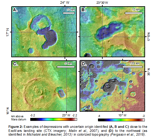
Acknowledgments: This research is a contribution of the Project ”MarsFirstWater”, European Research Council Consolidator Grant no. 818602. The authors also thank the Agencia Estatal de Investigación (AEI) project no. MDM-2017-0737 Unidad de Excelencia ”María de Maeztu”, and Rey Juan Carlos University.
References:
Christensen P. R. et al., Space Sci Rev. 110, 85–130 (2004).
Christensen P. R., R. L. Fergason, C. S. Edwards, J. Hill, in LPSC, 44, No. 1719, id. 2822 (2013).
Davis J. M., M. Balme, P. M. Grindrod, R. M. E. Williams, S. Gupta, Geology. 44, 847–850 (2016).
Davis J.M. et al, J Geophys Res Planets. 124(7), 1913–1934. (2019).
Dickson J. L. , L. A. Kerber, C. I. Fassett, B. L. Ehlmann, in LPSC, 49, No. 2083, id. 2480 (2018).
Fergason R. , T. Hare, J. Laura, Astrogeology PDS Annex, US Geological Survey (2018).
Hynek B. M., M. Beach, M. R. T. Hoke, J Geophys Res Planets. 115 (2010).
Jaumann R. et al., Planet Space Sci. 55, 928–952 (2007).
Malin M. C. et al., Journal of Geophysical Research: Planets, 112, E5 (2018).
Michalski J. R. , J. E. Bleacher, Nature. 502, 47–52 (2013).
Molina A. et al., Icarus. 293, 27–44 (2017).
Molina A., O. Prieto-Ballesteros, I. López, C. Robas, A. G. Fairén, in EANA Conf., 282577 (2019).
Ramsdale J. D. et al., Planet Space Sci. 140, 49–61 (2017).
Robas C., A. Molina, I. López, O. Prieto-Ballesteros, A. G. Fairén, in EANA Conf., 280888 (2019).
Voelker M., J. D. Ramsdale, in Planetary Cartography and GIS, H. Hargitai, Ed. (Springer International Publishing, Cham, 2019), pp. 293–302.
How to cite: Molina, A., Robas, C., Voelker, M., López, I., de Pablo, M. Á., Prieto-Ballesteros, O., and G. Fairén, A.: Grid mapping survey for water- and volcanic-related features along Arabia Terra in the context of the ExoMars landing site, Europlanet Science Congress 2020, online, 21 Sep–9 Oct 2020, EPSC2020-969, https://doi.org/10.5194/epsc2020-969, 2020.
MarsSI (“Mars Système d’Information”, french for Mars Information System) is a platform and service to catalog, process and retrieve data from orbiters. https://marssi.univ-lyon1.fr/MarsSI.
1. Introduction
Geological investigations of planetary surfaces require the combination of orbital datasets. Missions being often multiple-instruments platforms from multiple space agencies, the quantity of data available increased quickly.
MarsSI [3] is a platform designed to explore, calibrate, process and retrieve Mars orbital data. It was certified in 2017 as french national Research Infras- tructure by the Centre National de la Recherche Scientifique (CNRS) as part of the Planetary Surface Portal (PSUP) [2].
As of 2020, it indexes the optical (visible, multi and hyper-spectral) data from the recent orbiter missions, and allow to request the creation of Digital Elevation Models on demand. The focus, as highlighted by figure 1 is to allow the user to browse and request ”ready-to-use” products in regards of calibration, refinements and georeferencing. The user will be able to visualize and interpret the data in GIS or remote sensing software.
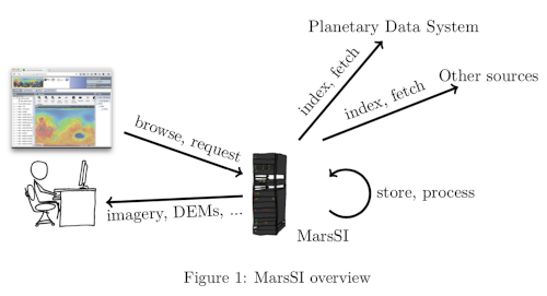
2 Architecture
MarsSI’s hardware is hosted at the Université Lyon 1 and is composed of a frontend server, a storage bay and a 80 core cluster. The software stack heavily relies on the OGC-defined standards for interoperability between components.
2.1 Catalog
MarsSI retrieve the footprints provided by the NASA Planetary Data System (PDS) in a database. These footprint information, alongside rasters that will be used as layers of our map display, is made available through a Mapserver instance. One issue we faced is the lack of Coordinates Referencing Systems definitions readily available in the WMS/WFS protocols, who rely on EPSG definitions codes. Adding and using non-standard EPSG definitions was a workaround to this issue.
Once the catalog, we proceed over the CTX and HiRISE data collections to find for each dataset overlapping images by at least 60% and a maximum differ- ence of acquisition angle of 10° to generate a list of potential Digital Elevation Models (DEMs).
2.2 Pipelines
Alongside the catalog, MarsSI uses several processing pipelines. Those pipelines defines steps and procedures to fetch, calibrate and refine products. A notable pipeline is the use of the Ames Stereo Pipeline [1] software to generate on- demand DEMs.
The pipeline execution is managed using the OAR (oar.imag.fr) batch scheduler.
One design choice of MarsSI was to present the products, including those created by the service, as global to all users (in contrast to service creating user-specific products). This was done to have only one reference to products like generated DEMs and reduce storage use. As a result, we only designed fully automated pipelines.
2.3 Frontend
MarsSI client interface is a web component based on Geomajas (www.geomajas. org), a free and open source GIS toolkit. Geomajas interface directly with the mapserver instance and provide widget for the main interface, shown on figure 3.
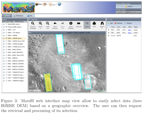
3 Usage and data volumes
MarsSI is open to the scientific communities around the world. As of june 2020, we count 294 registered users across more than 128 institutes. Storage-wise, we benefited to progressively download data as requested, reaching 34To in 2020.
4 Perspectives
We are currently working on integrating other data types in MarsSI, such as the MARSIS and SHARRAD radar datasets.
Another aspect we are working on is a more efficient and intuitive web in- terface not based on Geomajas. The rewrite would also take into account other maps such as polar projections and other planetary bodies.
As DEMs are our most requested products, we are investigating how to pro- vide qualitative assessment for those datasets. We are also looking for methods to generate large scale DEMs using mosaicking.
5 Conclusion
Built upon frameworks using standardized protocols, MarsSI offers the scientific communities a way to search and request data, most notably DEMs that can be derived from CTX and HiRISE data collection. We are now looking to modernize and extend the service with a newer interface that can present other planets and moons data.
Acknowledgments
MarsSI is a national Research Infrastructure, recognised as such by the French Ministry of Higher Education and Research. It was supported by the Pro- gramme National de Planétologie (PNP) of CNRS/INSU, co-funded by CNES. It was initialy supported by the European Research Council under the European Union’s Seventh Framework Program (FP7/2007-2013)/ERC Grant agreement No.280168.
References
[1] Zachary M Moratto et al. “Ames Stereo Pipeline, NASA’s open source automated stereogrammetry software”. In: Lunar and Planetary Science Conference. Vol. 41. 2010, p. 2364.
[2] François Poulet et al. “PSUP: A Planetary SUrface Portal”. In: Planetary and Space Science 150 (2018), pp. 2–8.
[3] C. Quantin-Nataf et al. “MarsSI: Martian surface data processing informa- tion system”. In: Planetary and Space Science 150 (2018), pp. 157 –170. issn: 0032-0633. doi: https://doi.org/10.1016/j.pss.2017.09. 014. url: http://www.sciencedirect.com/science/article/pii/ S0032063316304718.
How to cite: Volat, M., Quantin-Nataf, C., Thollot, P., and Mandon, L.: MarsSI: Martian surface data processing service, Europlanet Science Congress 2020, online, 21 Sep–9 Oct 2020, EPSC2020-564, https://doi.org/10.5194/epsc2020-564, 2020.
Introduction
In 2023 the Rosalind Franklin rover will land on Mars at Oxia Planum, as part of the European Space Agency’s ExoMars programme. Transverse Aeolian Ridges (TARs), periodic bedrock ridges (PBRs), dust devils, dust devil tracks, and/or windstreaks are common within the rover’s landing ellipse. These aeolian features can be used to characterize the paleo and contemporary aeolian environment of the landing region before the start of rover operations. Here we present new measurements of the orientation, morphologies, and directionality of TARs, PBRs, windstreaks, and active dust devils, in order to better understand the wind regime at the landing site, on a continuum of spatial and temporal scales.
Methods
We used machine learning (Novelty or Anomaly Hunter – HiRISE [NOAH-H])[1] and manual mapping-derived TAR and PBR distributions, as well as feature orientation and crest-line lengths to elucidate regional wind patterns in a 640 km2 area of Oxia Planum (Fig.1). The area was gridded into 160 four km2 quadrants, with every second quadrant analyzed. TAR crestlines were manually digitized as continuous and discontinuous ripples, based on NOAH-H ontological classes (Barrett et al., in prep). Continuous ripples are found at a variety of scales (metres to tens of metres in across-bedform length) and consist of patches of parallel ripples which merge into one another. Discontinuous ripples are features in which the aeolian bedforms are separated by areas of non-aeolian material, including those that are isolated on the surface and those which form part of a sparse patch overlying any non-aeolian material. PBRs were identified based on NOAH-H bedrock classes, as well as their morphology and texture, similar to PBRs found elsewhere on Mars[2] and Earth[3].
We used multiple change detection techniques on HiRISE, HRSC, and CaSSIS imagery to determine migration rates of TARs and to track active dust devils and analyze wind streaks [4-8].
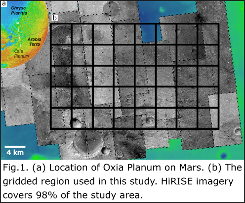
Results and Discussion
We digitized the crestlines of 7989 continuous ripples and 2764 discontinuous ripples. TAR along-crestline lengths range from 1.1 m to 556 m. Meter-scale TARs are common across the study area but decameter-scale TARs are uncommon, and are primarily found in topographic lows. Irrespective of the scale of the bedform, we found crestline azimuths to be consistent across the study area. Based upon terrestrial megaripple research using the difference in albedo to determine the stoss and lee slopes of ripples in the Argentinian Puna[9], coupled with the crestline azimuths determined from digitizing the landforms, we posit that the winds responsible for the expression of TARs in Oxia Planum blew from the NW-NNW towards the SE-SSE (Fig.2). Crestlines for 457 PBRs were digitized, and found to be longer than TAR crestline-lengths: PBRs have ridge-crests that range in length from ~4 m to just over 600 m. Azimuths of PBRs were found to be substantially different than TARs, requiring winds to have blown from the N-NNE or the S-SSE, accounting for 180° ambiguity. However, analysis of coregistered and orthorectified repeat HiRISE imagery over 11 Earth years showed no appreciable movement in TAR fields in the study area.
Two active dust devils were identified in the study area using HRSC images. One dust devil moved from the NW to the SE, while the second travelled from the SW to the NE. From a pair of CTX images taken 50 Earth days apart, 6 active dust devils and 649 dust devil tracks and/or windstreaks were identified. The features are predominantly oriented in a WNW-ESE direction with a secondary NEN-SWS noted for a few of the tracks (Fig.2).
The computed azimuths for TARs, PBRs, dust devils and dust devil tracks and/or windstreaks are markedly different (Fig.2), suggesting that different formative winds would have been necessary to result in the directionality of bedforms, landforms, and dust devils we currently see in Oxia Planum. These results pose important questions about the wind regime in this area. When were the winds responsible for TARs and PBRs active? And if contemporary winds are not responsible for TAR and PBR orientation, when did the wind regime shift? To begin answering these questions, our work will focus on comparing the results from this morphological study with modelled climate data in order to help determine when and why the wind regime changed.

Looking forwards to the surface mission, the surface platform for the Rosalind Franklin rover will carry a meteorological package that will provide in situ wind measurements. We can compare those data to our morphologically- and modelled-derived results. The rover itself will be able to analyze the granulometry of TARs and the bedrock strata of PBRs using imaging data, further assisting us to characterize the winds from a geomorphological standpoint. These datasets will provide further understanding of the aeolian regime of the Oxia Planum area and provide valuable insight into the climatic history of Mars.
References
[1] Barrett et al. (In Prep). NOAH-H, a deep-learning, terrain analysis system: results for the ExoMars Rover candidate landing sites.
[2] Montgomery et al. (2012). Journal of Geophysical Research: Planets, 117(E3).
[3] Hugenholtz et al. (2015). Aeolian Research, 18, 135-144.
[4] Balme et al. (2008). Geomorphology, 101(4), 703-720.
[5] Greeley et al. (2004). Geophysical research letters, 31(24).
[6] Leprince et al. (2007). IEEE Transactions on Geoscience and Remote Sensing, 45(6), 1529-1558.
[7] Reiss et al. (2011). Icarus, 215(1), 358-369.
[8] Grindrod et al (2018). Journal of Geophysical Research: Planets, 123(7), 1881-1900.
[9] Favaro et al. (2020). Icarus, 113765.
How to cite: Favaro, E. A., Balme, M. R., Davis, J., Grindrod, P. M., Fawdon, P., Barrett, A. M., and Lewis, S. R.: Aeolian Signals from landforms and bedforms at the Landing Site for the ExoMars Rosalind Franklin Rover in Oxia Planum, Mars, Europlanet Science Congress 2020, online, 21 Sep–9 Oct 2020, EPSC2020-572, https://doi.org/10.5194/epsc2020-572, 2020.
The ExoMars mission will deploy a stationary surface platform and a rover in Oxia Planum (OP), a region at the transition between the heavily cratered highlands of Mars and the ancient and filled impact basin, Chryse Planitia. While the fundamental geologic characteristics of the area have been investigated during the landing site selection process, detailed geologic or morpho-stratigraphic mapping is still missing. To fill this knowledge gap, two complementary mapping approaches were initiated by the ExoMars RSOWG: (1) Local HiRISE-scale mapping of the landing ellipse(s) area (reported elsewhere: Sefton-Nash et al., LPSC 2020). (2) Regional mapping at ~CTX-scale [this study] will provide a more synoptic view of the wider landing site within OP, enabling the contextualization of the units within the stratigraphy of western Arabia Terra and Chryse Planitia, and a comparison to other sites with similar key geologic and physiographic characteristics. It is also expected that this map will serve as a geologic reference throughout the mission and subsequent data analysis. The study area is located between 16.5°N and 19.5°N, and 334°E to 338°E. The data sets used for mapping include HRSC, THEMIS IR (day and night), CTX, and CaSSIS. Mapping scale in a GIS environment is 1:100,000, which will result in a final printable map at a scale of 1:1M.
Mapping started in mid-October 2019. Overall, the identified map units are very similar to those described by Quantin et al. (Astrobiology, submitted): The spatially most widespread units are the phyllosilicate-bearing unit that is the prime ExoMars target (with distinctly enhanced THEMIS nighttime temperatures when compared to its surroundings), a dark resistant unit of possibly volcanic or sedimentary origin, and a mantling unit that was likely emplaced by eolian processes. Multiple channels of various morphology and degradation state as well as sedimentary fan-shaped deposits (with low nighttime temperatures) imply a diverse and possibly long-lived history of surface runoff, perhaps accompanied or replaced by groundwater processes such as sapping. Inverted landforms (channels, impact craters) are the result of intense erosion. Additional mapped features include tectonic structures such as wrinkle ridges and lobate scarps (delineating a basin-like depression in the central mapping area), remnant erosional buttes in the northwestern portion of the mapping area (i.e. towards Chryse Planitia), craters and their ejecta blankets, and fields of eolian bedforms and secondary craters.
At the time of writing, the mapping is incomplete (partly cecause of the impact of the covid-19 crisis on the coordination of the joint mapping), and only initial and limited conclusions can be drawn. Overall, the mapping confirms previous geologic analyses. However, some features (e.g., contractional structures, channels, possible sapping landforms) need further attention as the may provide important constraints on the tectonic and aqueous evolution of the ExoMars landing area. A comparison to a distant, but geologically very similar site in Xanthe Terra, southeast of the Hypanis fan-shaped deposits, may enable testing of hypotheses raised by the geologic mapping of Oxia Planum.
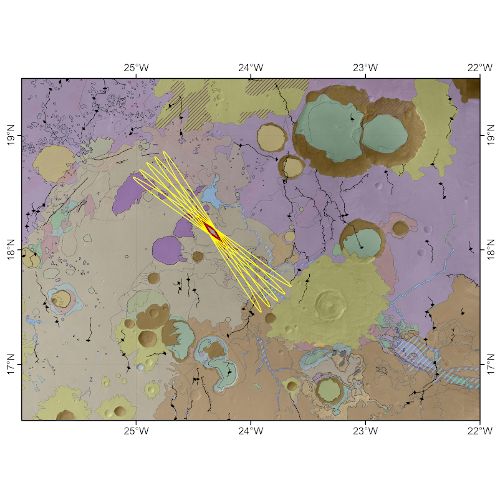

How to cite: Hauber, E., Adeli, S., Tirsch, D., Nass, A., Acktories, S., and Steffens, S.: Regional Geologic Mapping of the Oxia Planum Landing Site for the Exomars Mission, Europlanet Science Congress 2020, online, 21 Sep–9 Oct 2020, EPSC2020-1100, https://doi.org/10.5194/epsc2020-1100, 2020.
Planetary remote sensing (RS) missions are returning an ever increasing volume of data from across the Solar System. This wealth of data, much of it with a high spatial resolution, presents major challenges as well as opportunities. It is becoming increasingly difficult to fully interrogate large RS datasets such as the High Resolution Imaging Science Experiment (HiRISE) images of Mars (McEwen et al. 2010). The time required to survey all relevant images at full resolution can be daunting for all but the largest teams.
Advances in machine learning provide a way to overcome these challenges, by automating the initial surveying of planetary RS data, and providing a more accessible dataset, which highlights textural features of interest to the project.
The Novelty or Anomaly Hunter – HiRISE employs a deep learning convolutional neural network (DNN) to classify HiRISE images (LeCun et al. 2015; Simonyan and Zisserman 2015; He et al. 2016). A set of ontological classes was designed, which covered the complete range of textures at the site. These consisted of broad “terrain types” rather than formal geomorphological units. The aim of the project was to classify the Exo-Mars Rosalind Franklin Rover (Vago et al. 2017) landing site, and identify features such as aeolian bedforms or blockfields which might present localised hazards to rover operations (e.g. Rothrock et al. 2016). This would provide a useful input to traversability analysis. The focus was thus on detection, rather than digitisation. Producing a formal geomorphological map was beyond the scope of the project.
Four broad categories of classes were selected; non-bedrock surfaces, bedrock surfaces, aeolian bedforms, and boulder fields.
The surface classes were subdivided in terms of their metre scale relief and apparent roughness upon visual inspection. Bedrock classes exhibited clearly defined texture and relief, suggestive of outcrops, while non-bedrock was interpreted to consist of regolith or loose materials. Both were further subdivided according to the degree to texture present.
The bedform classes were distinguished from the non bedrock surfaces by the presence of clear aeolian ripple forms (Balme et al. 2008; Balme et al. 2017). They were subdivided based upon both the scale of the bedforms, and whether they were continuous or discontinuous. Large isolated ripples were labelled individually, but this was not practical for large fields of smaller discontinuous ripples. These were thus classified based on whether they overlaid bedrock, or non bedrock surfaces. A very small number of sites within the study area also exhibit rectilinear ripples. These were only found on a large scale.
Finally boulder patches consist of block fields, and regions of boulder strewn ground. Individual blocks were too small to label, so patches of boulder covered ground were classified.
These classes were used to manually label a set of ~1500 training images, each being a small 128-128m “framelet” extracted from the larger HiRISE image. From these examples, the DNN learned to classify the entire site according to the prescribed classification scheme. The model output consisted of a classified raster image, of the same dimensions as the original HiRISE image. This was colour coded and overlain on the HiRISE images for further analysis.
NOAH-H performed very well when identifying the very distinct classes such as bedforms, boulder fields and areas of fractured ground. Distinguishing between surface classes proved less reliable. This is likely due to the fact that many of these classes form a continuous variation, and so cannot be divided into discrete types with 100% reliability. When similar classes are grouped, and all bedrock or non bedrock terrains are considered together, the reliability of the model increased dramatically.
The majority of confusion occurred within these broader groups, rather than between them. The final run of the model produced a mean Intersection over Union (IoU) of 74.15% for the full class list and 92.33% for the grouped classes.
A set of sample locations were also studied to determine how the geomorphology was represented in the output data. This analysis broadly supported the results of the IoU analysis. The pixel scale results were not always found to be a perfect match, due to subtle variations within and between classes. The model sometimes struggled with “fuzzy” boundaries between regions of contrasting terrains.
However, it was found that even in cases where some individual pixels were misclassified, the classification of the area as a whole was frequently still both useful and reliable. While only 53% of sampled locations were found to be correctly classified at the pixel scale, 72% were correct when the landscape of the area as a whole was considered. When classes were combined into groups, this increased to 88% of the sampled locations.
The model results are thus most useful when considered at the “landscape scale”. It provides a very reliable guide to the distribution of terrains within an area and will provide a valuable tool for geomorphological study. It is already being applied to detection of aeolian hazards at the Oxia Planum site (See: EPSC2020-572).
References
Balme M, Berman DC, Bourke MC, Zimbelman JR (2008) Transverse Aeolian Ridges (TARs) on Mars. Geomorphology 101:703–720. doi: 10.1016/j.geomorph.2008.03.011
Balme M, Robson E, Barnes R, et al. (2017) Surface-based 3D measurements of small aeolian bedforms on Mars and implications for estimating ExoMars rover traversability hazards. Planet Space Sci 153:39–53. doi: 10.1016/j.pss.2017.12.008
He K, Zhang X, Ren S, Sun J (2016) Deep Residual Learning for Image Recognition. Proc. IEEE Conf. Comput. Vis. Pattern Recognition,. pp 770–778
LeCun Y, Bengio Y, Hinton G (2015) Deep learning. Nature 521:436–444. doi: 10.1038/nature14539
McEwen AS, Banks ME, Baugh N, et al. (2010) The High Resolution Imaging Science Experiment (HiRISE) during MRO’s Primary Science Phase (PSP). Icarus 205:2–37. doi: 10.1016/j.icarus.2009.04.023
Rothrock B, Kennedy R, Cunningham C, et al. (2016) SPOC: Deep Learning-based Terrain Classification for Mars Rover Missions. AIAA Sp 2016. doi: 10.2514/6.2016-5539
Simonyan K, Zisserman A (2015) Very deep convolutional networks for large-scale image recognition. 3rd Int. Conf. Learn. Represent. ICLR 2015 - Conf. Track Proc. pp 1–14
Vago JL, Westall F, Coates AJ, et al. (2017) Habitability on Early Mars and the Search for Biosignatures with the ExoMars Rover. Astrobiology 17:471–510. doi: 10.1089/ast.2016.1533
How to cite: Barrett, A. M., Balme, M. R., Woods, M., Karachalios, S., Petrocelli, D., Sefton-Nash, E., and Joudrier, L.: NOAH-H, a deep-learning, terrain classification system for HiRISE: Results for Oxia Planum and Mawrth Vallis., Europlanet Science Congress 2020, online, 21 Sep–9 Oct 2020, EPSC2020-676, https://doi.org/10.5194/epsc2020-676, 2020.
Introduction
Oxia Planum is a clay-rich plain located on the boundary between Arabia Terra and Chryse Planitia, and will be the landing site of the ExoMars 2022 rover, ‘Rosalind Franklin’. The region is situated between the ancient, rugged terrain of the southern highlands, and the young, smooth plains of the northern lowlands; in effect, the area acts as part of a transitional zone between the two hemispheres of the planet. Distributed across the Oxia and Circum-Chryse regions are thousands of kilometre-scale isolated landforms that resemble terrestrial mesas, buttes, hills, and plateaus (Figure 1). As a widespread geomorphological feature in this highland-lowland transitional area, they are important in the geological history of the region, but their origins are not well understood and are not yet documented. This study investigates the morphologies and distributions of the mounds in order to improve our understanding of their mode of formation and place in the regional stratigraphy.
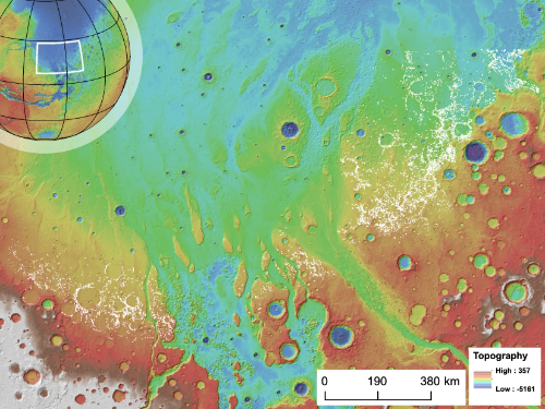
Figure 1: Study area showing the location of mounds (white dots) in Chryse Planitia.
Data and Methods
14,346 mounds were identified and investigated within a study area of ~500,000 km2 using an HRSC (High Resolution Stereo Camera; Jaumann et al., 2007) and orthorectified CTX (Context Camera; Malin et al., 2007) base map that was incorporated into an ArcMap GIS (Geographical Information Systems) environment. The mounds were identified by manual inspection and were distinguished from subjacent plains by their characteristic high albedo and low thermal inertia. Mound margins and prominences (such as peaks and plateaus) were identified by their visible morphology and were digitised by hand. A circular buffer of 100 m radius was generated around mound apexes, and a 200 m buffer generated around the lower mound margin in order to accurately capture the relief of the surrounding topography. Mound height was determined by extracting the maximum elevation of the mound tops and the mean elevations of the surrounding plains from the MOLA PEDR (Mars Orbiter Laser Altimeter Point Experimental Data Records) (Zuber, 1992) and the HRSC Digital Terrain Model (DTM) raster data sets.
Results
Mounds are classified into four categories: (1) Hills have a single prominent peak or smooth crest (Figure 2a). (2) Mesas have a single plateau at its maximum elevation (Figure 2b). (3) Clustered mounds are instances where multiple hill peaks or mesa plateaus are juxtaposed, but the gap between them does not reach the elevation of the surrounding plains (Figure 2c). (4) Compound mounds are when hills or mesas appear to be vertically stacked on top of one another, forming distinct tiers (Figure 2d). MOLA and HRSC-derived measurements reveal that the heights of the mounds increase with areal extent, up to a maximum of ~500 m, after which the height does not increase further. This maximum height limit is reached when mounds have an area of ~10km2 in area (Figure 3).
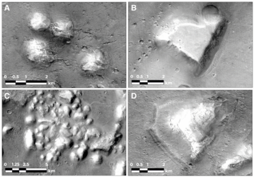
Figure 2: Examples of mounds (CTX): A: Hills, B: Mesa, C: Clustered Mounds, D: Compound Mounds.
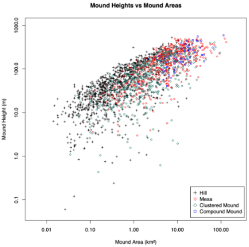
Figure 3: Graph showing the relationship between height and area for 2366 mounds of different classes.
Discussion
Mounds with clear, regolith-free margins show compelling evidence for being mantled and embayed by the dark plains material mapped as the HNCC1 and HCC2 units by Tanaka et al. (2005). They therefore predate the Late-Noachian to Early-Hesperian emplacement of these units. In the Oxia Planum region, the mounds directly overlie the Early Noachian (Quantin-Nataf et al., 2020) clay-bearing units. This suggests that the mounds were deposited—and partially eroded—between the Early and Late Noachian.
The morphology and morphometry of a given mound are an expression of its erosional condition (Figure 3). Hills, with their rounded appearances, have the lowest average heights and have clearly been eroded more than the flat-topped mesas, which include some of the tallest mound examples. Compound mounds are intermediate in both morphology and height, suggesting that they represent a transitional erosional state between hills and mesas, and that the population represents the remnants of an eroded layer. The population of mounds extends several hundred kilometres into the northern lowlands, implying that the layer the mounds formed from (if this is their origin) once covered a substantial amount of the northern lowlands, proximal to the dichotomy boundary.
Many of the mounds in the study area occur in curvilinear or ring-like arrangements, which are suggested to demarcate the location of underlying buried craters (Rodríguez et al., 2007). The preferential occurrence of mounds around the edges of buried impact craters implies that these areas were commonly more resistant to the erosion that created the mounds’ present-day relief. We suggest that these crater margin-delineating mounds are the result of post-impact hydrothermal/groundwater activity that exploited pre-existing impact-generated fractures. This process would have reinforced the material directly above the fractures through the precipitation of minerals that increased the mechanical competence of the superimposing ‘mound’ layer. Subsequent differential erosion then removed the non-indurated material, leaving arcuate patterns of mounds above crater-edges. Many mounds do not occur in arcuate patterns. We attribute these to localised fractures in the underlying bedrock that acted as individual conduits for fluid flow, or to craters that have had most of their mounds buried or removed through erosion.
Conclusions
Through studying the morphology, morphometry and distribution of mounds of Chryse Planitia we show that: (1) We have identified 14,346 mounds in the south Circum-Chryse region. The mounds can be divided into 4 classes, hills (isolated, rounded top), mesas (isolated flat topped), clustered mounds (non-isolated hills or mesas) and tiered mounds (stacked mesas and hills). (2) The height–area relationship of the mounds plateaus at a maximum of ~500 m. Combined with the observation of the degree of erosion of different mound morphologies, this result suggests that the mounds formed from at least one layer that was regionally extensive in the past. (3) The local distribution of mound-associated buried impact structures supports hydrothermal activity as part of the preferential preservation process.
How to cite: McNeil, J., Balme, M., Fawdon, P., and Coe, A. L.: Morphology, Morphometry, and Distribution of Isolated Landforms on the Margin of Chryse Planitia, Mars, Europlanet Science Congress 2020, online, 21 Sep–9 Oct 2020, EPSC2020-216, https://doi.org/10.5194/epsc2020-216, 2020.
Abstract
The WISDOM ground penetrating radar aboard the Rosalind Franklin rover of the ExoMars 2022 mission will provide radar images of the Martian shallow subsurface down to a few meters and with a vertical resolution of a few centimetres. Such a high resolution imaging of the subsurface will be key in understanding the geological context and guiding the sample acquisition by the rover’s drill. In order to enhance WISDOM resolution and meet the desired 3-cm value (the length of the samples that will be collected), a super-resolution technique known as the “Bandwidth Extrapolation” (BWE) is applied to WISDOM data. The BWE is validated on synthetic and laboratory data before being applied to observations acquired in a variety of potential Martian analog environments.
1. Range resolution and the BWE technique
The ExoMars 2022 rover mission is the first mission in the history of the robotic exploration of Mars able to collect 3cm-long samples down to 2 m below the surface [1]. The data collected by the WISDOM radar will be processed to produce images (radargrams) of the subsurface, that will be interpreted in terms of geological structures and provide constraints on the subsurface composition. WISDOM radargrams will bring insights into the geological context and evolution of the landing site, and eventually, guide the drilling operations [2]. The WISDOM flight model has been calibrated [3] and an improved version of the data processing pipeline is being developed.
WISDOM is a stepped-frequency radar operating at a central frequency of 1.75 GHz over a wide frequency bandwidth B (2.5 GHz). An Inverse Fourier Transform (IFT) is applied to the data to construct a response in time-domain. WISDOM range resolution 𝛿𝑟 is limited by the width of the synthetic pulse obtained in time domain, which is inversely proportional to the effective bandwidth of the instrument. 𝛿𝑟 also depends on the dielectric constant of the sounded medium 𝜀𝑟. Typically, for a pulse width at 6dB,
![]()
Windowing (a technique commonly used with IFT to reduce side-lobes) further degrades the resolution, to ~1.5 𝛿𝑟 for a Hamming window function. As a result, the vertical resolution of WISDOM radargrams in a subsurface with a typical dielectric constant of 4 after windowing would become ~5.4 cm which is slightly larger than the expected ~3.6 cm without windowing, and higher than the desired 3 cm.
In order to improve WISDOM range resolution, we implemented a processing technique developed at the Lincoln laboratory of the MIT in 1977: the Bandwidth Extrapolation (BWE) [4]. The BWE has already been successfully applied to planetary data from radars, such as MARSIS/Mars Express [5], SHARAD/MRO [6], and the Cassini radar [7], [8]. We have adapted it for implementation in the data processing pipeline of WISDOM. The BWE technique extrapolates a radar frequency spectrum with an autoregressive linear model of the signal [9] before IFT to increase its bandwidth [10], and therefore improve its resolution in time-domain. An enhancement by a factor of 3 can be achieved [11], leading to a new range resolution better than 2 cm for a dielectric constant of 4.
2. Validation and application on potential Martian analogs
The BWE was first validated on synthetic soundings simulating echoes from two reflectors separated by different distances with an additive white noise, to assess its ability to improve the resolution in distance while preserving the time delays and amplitudes values of the two corresponding echoes. The method was then applied to WISDOM experimental data acquired in semi-controlled environments, where the different reflectors’ location is known prior to sounding. Doing so, we confirmed that the BWE leads to a significant resolution enhancement, up to a factor 3, before applying the technique to various sets of data acquired in relevant Martian analog environments.
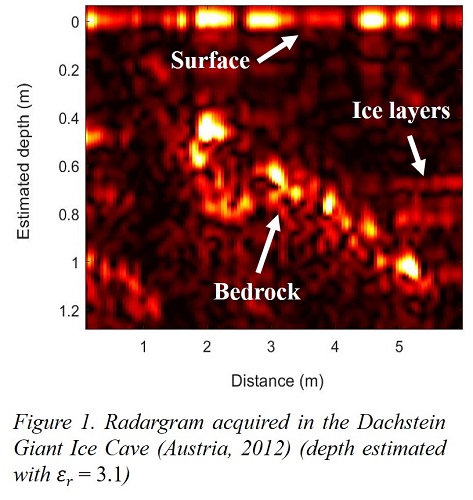
As an illustration, Figure 1 presents a radargram acquired in the Dachstein Giant Ice Cave (Austria, 2012), showing a bedrock beneath a layered ice-sheet [12], and Figure 2 the improved version after application of the BWE. The resolution is enhanced by a factor of 3 which greatly eases the detection and interpretation of buried structures. Further, new details are revealed. Other tested environments include a French Alps layered snowpack and pyroclastic deposits in the flanks of the Etna.
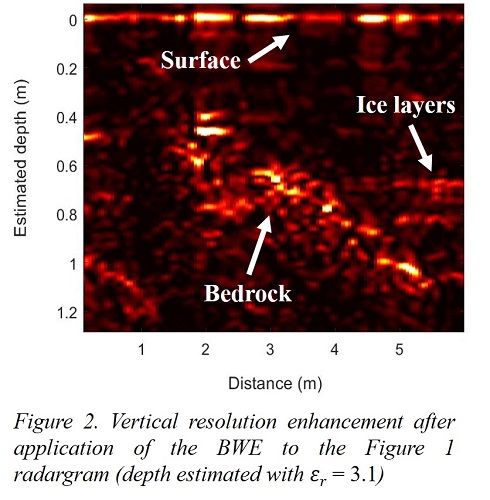
On Mars, the BWE technique will be a powerful tool to search for structures such as layered deposits or the buried part of an outcrop, and to detect buried boulders the rover drill must avoid.
3. Conclusion and perspectives
The implementation of the BWE super-resolution technique proved to bring an improvement of the range resolution by a factor of 3 in WISDOM radargrams. The use of this technique will be key in the interpretation of future radargrams acquired on Oxia Planum [13], landing site of ExoMars 2022, and to accurately determine the depth to be sampled by the drill. On-going work is dedicated to adapt BWE to the full polarimetric WISDOM dataset and to propose improved algorithms for an even more accurate bandwidth extrapolation.
Acknowledgments
This research is funded by the CNES and the UVSQ.
References
[1] J. L. Vago et al., Astrobiology, 2017.
[2] V. Ciarletti et al., Astrobiology, 2017.
[3] Y. Hervé et al., Planet. Space Sci., 2020.
[4] S. B. Bowling, MIT Lincoln Lab., 1977.
[5] M. C. Raguso et al., European Signal Processing Conference, 2018.
[6] M. C. Raguso et al., 5th IEEE International Workshop on Metrology for AeroSpace, 2018.
[7] M. Mastrogiuseppe et al., Geophys. Res. Lett., 2014.
[8] V. Poggiali et al., IEEE Trans. Geosci. Remote Sens., 2019.
[9] J. P. Burg, 37th Meet. Soc. Explor. Geophys., 1967.
[10] K. M. Cuomo, MIT Lincoln Lab., 1992.
[11] T. Moore et al., Lincoln Lab. J., 1997.
[12] S. Dorizon et al., Planet. Space Sci., 2016.
[13] C. Quantin-Nataf et al., Ninth Int. Conf. Mars 2019, 2019.
How to cite: Oudart, N., Ciarletti, V., Le Gall, A., Mastrogiuseppe, M., Hervé, Y., Benedix, W.-S., Plettemeier, D., Tranier, V., Hassen Khodja, R., Statz, C., and Lu, Y.: Resolution enhancement of WISDOM/ExoMars radar soundings applied on potential Martian analogs, Europlanet Science Congress 2020, online, 21 Sep–9 Oct 2020, EPSC2020-39, https://doi.org/10.5194/epsc2020-39, 2020.
On Earth, electric discharges in thunderstorms produce ELF waves in the Earth-ionosphere waveguide that circles the globe. These waves give rise to Schumann resonances in the waveguide resonant cavity. These waves are also expected to occur at Venus, produced by strong lightning in the Venus atmosphere and at Mars produced by active dust devils or dust storms, during southern hemisphere summer, when the planet is near periapsis. Within dust storms, dust particles undergo triboelectric charging. The charge transfer leads to charge separation. A lightning discharge is expected to occur when the charge exceeds the breakdown strength of the media present. The transient electric discharge emits electromagnetic waves in the VLF/ELF range of frequency, leading to Schumann Resonance in the surface-ionospheric cavity. In a heterogeneous cavity, Schumann resonance modes are observable using an in-situ instrument. Recently has it been possible to search for these electromagnetic waves from the Mars surface using the UCLA-provided InSight fluxgate magnetometer. The weakness of the vertical component of ULF waves at Mars suggests that the subsurface is electrically conducting, allowing trapping of electromagnetic energy between the sub-surface and the ionosphere. The fundamental mode of Schumann resonance carries higher energy compared to there are more chances of observing the fundamental mode. Various values of the first mode are predicted in the literature for Mars like 13-14 Hz or between 9-14 Hz and 17.5 Hz. Even if the fundamental mode is above 10 Hz, the 20 Hz sampling rate will allow detection of an aliased signal. We examine the data obtained during Martian sandstorms for the possible existence of such waves. A large dust storm was detected on Mars beginning on InSight sols 40 to 50, and ending during sols 50 to 90. Examining the 20 Hz InSight magnetometer data during this period reveals no clearly identifiable Schumann Resonance signals within the bandwidth of the magnetometer.
How to cite: Yu, Y., Russell, C., Chi, P., Haider, S., Pabari, J., and Luhmann, J.: Search for Martian Schumann Resonances, Europlanet Science Congress 2020, online, 21 Sep–9 Oct 2020, EPSC2020-541, https://doi.org/10.5194/epsc2020-541, 2020.
Introduction: The transport of ice by wind plays a major role in the surface mass balance of polar caps [1, 2]. Ice can be redistributed by wind due to (1) transport of ice particles and/or (2) transport of water vapour associated with sublimation/condensation. On Mars, although the low atmospheric density is less favourable for the transport of particles than on Earth, both dust and sand have been observed to be transported by wind [3,4]. Despite ice aeolian landforms have been observed at the surface of the North Polar Cap of Mars [2, 5, 6], ice particle transport has not been directly observed on the Martian surface. Similarly, no laboratory studies of snow/ice particle transport under Martian-like conditions have been attempted thus far due to the complexity of the material. In this study we performed experiments of ice particle transport in a wind-flow under low temperatures and low pressures. From the experiments, threshold shear velocity of water ice particle transport is retrieved for different pressures and sizes in order to evaluate the plausibility of ice particle wind-driven transportation at the surface of Mars.
The North Polar Cap of Mars: The Martian atmosphere is thin (7 mbar), cold (220 K) and dry (< 80 μm-pr) [7]. These conditions favoured ice sublimation/condensation processes. Spectral analyses [8, 9] suggested the optical ice grain sizes to vary between 10 μm to about 2000 μm for the seasonal frost and surface of the perennial North polar cap. But, the mechanisms of ice deposition are not well established. It can potentially come from vapour condensation directly onto the surface [9] or from snow fall [10]. This will affect the shape and size of ice particles and degree of ice sintering, which all influence the shear velocity threshold. The North polar cap experiences a permanent katabatic wind regime [11] with a typical friction shear velocity u* about 0.2 m.s-1. The complex interaction between the cryosphere and the wind leads to the formation of aeolian features at different scales [2, 5, 6].
Wind tunnel experiments: We performed experiments using the environmental wind tunnel AWTSII at Aarhus University. It is a cylindrical vacuum chamber, housing a recirculating wind tunnel about 8 m long, 2 m wide and 1 m high [12]. The facility can achieve a turbulent boundary layer flow at both low temperature and low pressure. The ice samples were produced by using the Setup for production of Icy Planetary Analogues [13]. The ice samples were sieved (125 - 250 μm, 250 - 500 μm, 500 - 2000 μm) as a monolayer on a plate covered with volcanic regolith (125 μm). The fan speed was increased by steps (shear velocity u* = 0 to 2 m.s-1) and the wind flow characterized by laser Doppler anemometry. The removal of ice particles was monitored by webcam. We performed the experiments for the different particle shapes and sizes for 4 different air pressures; 40, 100, 500 and 1000 mbar. The air temperature was maintained low (~-25°C) close to the sample plate to prevent the ice melting, sublimating and sintering.
Threshold shear velocity calculation: The threshold shear velocity was determined from analysis of acquired images. When bright ice particles are removed from the dark volcanic regolith plate, the reflectance of the surface decreases. Black and white reference targets are placed close to the sample plate in the field of view of the webcam. The reflectance evolution of a region of interest (ROI) on the sample plate is calculated as follow:
reflectance = (ROI – black target)/(white target – black target)
The reflectance serves as a proxy for ice mass removal. For each image the reflectance is linked to the corresponding shear velocity. In most of the cases performed, the reflectance is constant until a certain wind speed and then decreases. To determine the threshold shear velocity uth, we set the threshold reflectance at 10% decrease from the first image at u* = 0 m.s-1.
Results and conclusion: We have performed for the 1st time experiments of ice particles transportation at low pressure in a planetary wind tunnel. The averaged threshold shear velocity obtained at 1000 mbar, uth = 0.4 m.s-1, is consistent with theoretical and experimental calculation of ice/snow at terrestrial condition [14, 15], from 0.3 m.s-1 to 0.6 m.s-1 for range of ice particles sizes selected, supporting our set-up reliability. The shear velocity increases significantly as the pressure decreases. The influence of the ice grain sizes is not clear and more experiments are required. The results should then be scaled to Martian gravity in order to compare the results to wind speed simulations and conclude about the likeliness of transport of ice particles by wind at the surface of Mars.
References: [1] Das I. et al. (2013) Nature Geoscience, 6, 367-371. [2] Howard A. D. (2000) Icarus, 144, 267-288. [3] Cantor B. A. et al. (2010) Icarus, 208, 61-81. [4] Bridges B. A. et al. (2012) Geology, 40, 31-34. [5] Smith I. B. and Holt J. (2010) Nature, 465, 450-453. [6] Herny C. et al. (2014) EPSL, 403, 56-66. [7] Pankine A. A. et al. (2010) Icarus, 210, 5871. [8] Langevin Y. et al. (2005) Science, 307, 1584-6. [9] Appéré T. et al. (2011) JGR : Planets, 116, E05001. [10] Spiga A. et al. (2017) Nature Geoscience, 10, 652-657. [11] Spiga A. et al. (2011) PSS, 59, 915-922. [12] Holstein-Rathlou C. et al. (2014) Am. Met. Society, 31, 447-457. [13] Pommerol A. et al. (2019) Space Sci. Rev., 215. [14] Shao Y. and Lu H. (2000) JGR, 105, 437-443. [15] Clifton A. et al. (2006) JoG, 52, 585-596. [16] Herny C. et al. (2016) 6th MPSC, Abstract #6075. [17] Bordiec M. et al. (2018) ICAR X.
Acknowledgements: This work has been fund by Europlanet (Europlanet 2020 RI has received funding from the European Union's Horizon 2020 research and innovation program under grant agreement No 654208). This work has been supported by the University of Bern. This work has been carried out within the framework of the NCCR PlanetS supported by the Swiss National Science Foundation.
How to cite: Herny, C., Merrison, J., Iversen, J., Yoldi, Z., Bordiec, M., Carpy, S., Bourgeois, O., and Thomas, N.: Wind tunnel experimentation of ice particles transport in Martian-like environment, Europlanet Science Congress 2020, online, 21 Sep–9 Oct 2020, EPSC2020-343, https://doi.org/10.5194/epsc2020-343, 2020.
1. Introduction
New feldspar detections made by visible-near infrared spectroscopy this year on Mars [1], raise questions on the nature of the rocks involved and the magmatic processes responsible for their formation. Based on lunar studies, the presence of a 1.3 µm absorption band has been so far interpreted, as diagnosis of anorthosites containing more than 90% plagioclase [2]. However, these studies are based on VNIR spectra acquired in the laboratory, on binary mixtures of powders, containing Ca-plagioclase feldspar mixed with a mafic mineral such as olivine or pyroxene [3]. This paper presents our laboratory results regarding VNIR spectra measurements of several (uncrushed) terrestrial rocks containing feldspars of various compositions, in various amounts, and with different grain sizes as we expected all these factors to influence the spectral response. Our results allow us to survey in which cases the 1.3 µm band can be reproduced, and which are therefore possible analogue rock candidates. Finally, the sparse detections that have been recently made in the Valles Marineris region of Mars are compared with our library results.
2. Method
The objective of our study is to use VNIR reflectance spectroscopy to create a new reference spectral library containing reflectance spectra acquired on uncrushed terrestrial feldspathic rocks. Over 40 terrestrial feldspathic rocks of various types (volcanic, plutonic and metamorphic, Figure 1) were analyzed in this study.

Reflectance spectra of this wide range of rocks was measured with an ASD Fieldspec4 spectrometer in our laboratory. This instrument operates in three different wavelength ranges: VNIR (0.35 – 1 µm), SWIR 1 (1.001 – 1.801 µm), and SWIR 2 (1.801 – 2.5 µm), with a spectral resolution between 3 and 8 nm. Spectra were collected with the instrument bare fiber, contact probe, or Muglight. The distance of the fiber using accessories was ~ 15 mm from the rock, with a phase angle of ~45° and using an artificial light source. Approximately five different spectra were measured on each rock sample. Selected spectra are presented in Figure 2.

In parallel, Mars VNIR hyperspectral remote sensing data from the CRISM instrument (Compact Reconnaissance Imaging Spectrometer for Mars) onboard MRO (Mars Reconnaissance Orbiter) where feldspar signatures were recently reported [1] were analyzed. Raw data were downloaded from the PDS, corrected with the ENVI CAT (CRISM Analysis Toolkit) following the method described in [4] and then denoised using a custom-made routine [1].
Spectral criteria [5] are then computed to investigate whether or not an absorption band for a given wavelength was present. The BD1300 criteria was used in this study to highlight pixels which might contain a feldspar absorption band at 1.3 µm.
3. Results
Out of 42 measured analogue rocks, 18 rocks display absorption features around 1.3 µm. The rocks with positive 1.3 µm signatures include dacites, basalts, granodiorites, granites and diabase. Several spectra were measured on these rocks resulting in 82 positive spectra in our new spectral library (Table 1). The feldspar-bearing have absorption band centers varying from 1.15 to 1.4 µm.

A similar absorption is observed on eight analyzed CRISM cubes (Figure 2). The position of the center of the absorption band in the CRISM data is around 1.25 µm. If we compare the CRISM data to the spectra of our library, the right and left shoulders of the absorption band are very often equidistant from the center of the band, although the CRISM spectra here are limited at wavelengths >1 µm, making the left shoulder difficult to examine.
4. Discussion and Perspectives
Spectra collected on entire terrestrial feldspathic whole rocks show diagnosis plagioclase signatures which are similar to the ~1.3 µm absorption feature observed on Mars. Other candidate minerals, however, could show broad absorption bands centered between 1.1 and 1.3 µm, such as garnet, micas or volcanic glass. Still, spectral characteristics of both our library spectra and Mars CRISM spectra are more consistent with plagioclases.
Future work includes a detailed petrographic characterization of the analyzed samples. It is already shown, however, that some of our samples do not contain more than 40% plagioclase crystals and still display absorption band centered at 1.3 µm on the reflectance spectrum. These results are in contradiction with previous analysis of powder mixtures [6] which determined that the presence of 90% of calcic plagioclase is necessary in a rock for its band to be observable in a reflectance spectrum [3]. We argue that presence of an absorption band can also be influenced by the grain size which is an important factor to take into account: the larger the grain size, the deeper the absorption band, and most of our studied rocks do contain feldspar phenocrysts.
We conclude, from the comparison of our library spectra with the Mars CRISM spectra, that a range of effusive and cumulate rocks could correspond to the observed signatures. Previous studies suggested that these spectral signatures correspond to anorthositic primary crust [2], or felsic tertiary crust [7]. Although these hypotheses are plausible, our results suggest that it is virtually impossible to use feldspar detections to infer the presence of a primary or tertiary crust until we further constrain the true nature of the rocks and the exact geological context of these peculiar signatures.
5. References
[1] J. Flahaut et al. (2019). Goldschmidt Abstracts, 2019, 1010 (and article in prep.).
[2] J. Carter et al. (2013). Nature Geoscience, 6, 1008–1012.
[3] L.C. Cheek et al. (2014). American Mineralogist, 99(10), 1871-1892.
[4] S. Murchie et al. (2007). J. Geophy. Res, 112, E5.
[5] C.E. Viviano-Beck et al. (2014). Journal of Geophysical Research: Planets, 119, 1403–1431.
[6] D.A. Crown and C.M Pieter (1987). Icarus, 72(3), 492-506.
[7] V. Sautter et al. (2016). Lithos, 254-255, p.36-52.
How to cite: Barthez, M., Flahaut, J., Ito, G., Guitreau, M., and Pik, R.: Near-infrared laboratory measurements of feldspathic rocks as a reference for hyperspectral Martian remote sensing data interpretation., Europlanet Science Congress 2020, online, 21 Sep–9 Oct 2020, EPSC2020-606, https://doi.org/10.5194/epsc2020-606, 2020.
The Martian crust has long been thought to be made of relatively uniform FeO-rich mafic rocks but, over the last two decades, new meteorite discoveries, orbital and in-situ analysis of Martian rocks have painted a more nuanced picture. Alkaline rocks, silica-rich rocks and possible anorthosites have been identified at several locations [e.g., 1]. The basaltic rocks, still believed to account for the majority of the upper crust, also display a chemical variability that could be tied to the thermal-evolution of the planet’s interior [2]. Those various lithologies indicate that Mars had a rich geologic history and that the crust was shaped by a wide range of igneous processes.
The abundant basalts likely result from decompression melting of the upper mantle and represent a “secondary” crust that would have covered any “primary” crust formed during the crystallization of the magma ocean. The compositions of the melts transferred from the mantle to the crust are controlled by the pressure and temperature of melting and are best constrained with experiments [3]. However, experiments represent snapshots at fixed P-T and usually simulate isobaric batch melting processes that are not completely analogous to actual melting conditions in the mantle. An alternative is to use thermodynamic models [4, 5], which can be used to simulate polybaric and fractional melting. Unfortunately, those models show several important shortcomings. For example, pMELTS [4] systematically overestimates the FeO content of the melts produced at high pressure. To simulate partial melting of the Martian mantle, other workers have adopted a hybrid approach using pMELTS and corrections based on experiments [1-2]. This type of hybrid approach is still problematic because the magnitude of the offsets relative to experiments are pressure-dependent and larger than previously anticipated (e.g., up to 8 wt.% (Fig. 1a) vs. 3 wt.% [1-2] for FeO).
Here, we present a simple empirical model that reproduces the composition of experimental melts more accurately (Fig. 1b, 1d) and can also be used to simulate various melting behaviors. It is similar in concept to melting models developed for the near-fractional polybaric melting of the Earth mantle at mid-oceanic ridges [6]. The concentrations of minor and major incompatible elements (TiO2, Al2O3, Na2O, K2O and P2O5) into the melt are first calculated from experimentally determined partition coefficients between minerals and melt [3]. The concentration of the other major elements (SiO2, FeO and MgO) are then deducted from the concentration of incompatible elements and pressure. CaO is treated as a major compatible element or as an incompatible element, based on whether clinopyroxene is present in the residue (Fig. 1d).
The new empirical model calculates the composition of “instantaneous melts” formed by isobaric or polybaric continuous melting with an adjustable critical melt fraction (i.e. melt fraction retained in the residue). Compared to batch and aggregate melts (symbols and solid lines in Fig. 1), instantaneous melts (dashed lines in Fig. 1) become enriched in FeO, MgO and CaO and depleted in incompatible elements (e.g., K2O, Na2O, Al2O3) as melting progresses. Instantaneous melts can be pooled and directly compared to the composition of the Martian crust. They could also be used as input for more advanced modelling of igneous differentiation (e.g. involving fractional crystallization, magma mixing, etc.) to account for the formation of the more evolved Martian igneous rocks. In a future step, the new model will be used to incorporate an accurate treatment of compositional changes due to melting and depletion of the mantle in global thermochemical evolution models.
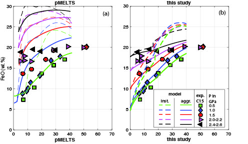
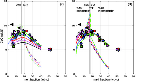
Fig. 1. Composition of mantle melts from a primitive mantle composition [7] at different but constant pressure (isobaric melting). (a, c) pMELTS model. (b, d) Empirical model. In this example, both models simulate continuous melting (near-fractional melting) with a 1% retained melt fraction. The dashed lines represent the “instantaneous melts” constantly removed from the residue. The solid lines represent the total pooled or “aggregate melts”, the sum of all previous instantaneous melts. Under isobaric conditions, aggregate melts are analogous to batch melts. Symbols (exp. C15) represent batch melts from the experiments of [3]. pMELTS accurately reproduces the experimental melt compositions at 0.5 GPa but not at higher pressure.
References:
[1] Sautter et al. (2015) Nat. Geosci. 10.1038/ngeo2474, [2] Baratoux et al. (2011) Nature 10.1038/nature09903, [3] Collinet et al. (2015) EPSL 10.1016/j.epsl.2015.06.056, [4] Ghiorso et al. (2002) G3 10.1029/2001GC000217, [5] Holland et al. (2018) J. Petrol 10.1093/petrology/egy048, [6] Till et al. (2012) JGR 10.1029/2011JB009044, [7] Dreibus and Wänke (1985) Meteoritics
How to cite: Collinet, M., Plesa, A.-C., Ruedas, T., and Breuer, D.: An empirical melting model for the Martian mantle , Europlanet Science Congress 2020, online, 21 Sep–9 Oct 2020, EPSC2020-1019, https://doi.org/10.5194/epsc2020-1019, 2020.
Introduction: Experimental studies showed that elevated phosphorus concentrations (> 1 wt. %) in terrestrial basaltic magmas have significant effects on the crystallization sequence, the composition and physical properties of melts [1-2]. [1] demonstrated that the polyvalent nature of P5+ favors the polymerization of silica tetrahedra, promoting the silica liquidus boundary in favor of that of pyroxene and the pyroxene liquidus boundary in favor of that of olivine. The enhancement of polymerized minerals can have significant implications regarding the petrogenesis of igneous rocks and mineralogy of the crust. Mars’ primitive mantle contains >10 times more phosphorus than Earth’s [3], which could result in considerable differences in magma compositions and crustal mineralogy between Earth and Mars.
Preliminary thermodynamical partial melting models based on a martian mantle composition using pMELTS software showed that phosphorus likely have implications in terms of magma compositions [4]. This study aims to explore with piston-cylinder experiments the effects of phosphorus on martian melt compositions and residual mineral assemblages when considering partial melting of a primitive mantle composition [6].
Methods: A set of nominally anhydrous partial melting experiments has been run on a primitive mantle composition [5] with two P2O5 contents (0 wt.% and 0.5 wt.%). We followed the exact same procedure as [6], which considered partial melting experiments in the same laboratory of a primitive mantle composition [5] with P2O5=0.2 wt.%, the actual mantle content. We will compare our results with those from [6].
Using oxides and carbonates, all reagents were fired to avoid any water contaminations, and mixed together using an agate motar for 2 hours. The mixture was then loaded in a graphite inner capsule, which was placed into a platinum outer capsule. Before welding shut the platinum capsule, the loaded capsule was dried at 300°C during 24 hours to minimize water contamination. The welded shut capsule was then emplaced into a crushable MgO internal spacers, cylindrical graphite furnaces, BaCO3 pressure sleeve, and the whole assembly was wrapped within a Pb-foil. A half-inch piston cylinder apparatus at Rice University has been used at a pressure of 2GPa and temperatures between 1210 and 1450°C during 24-72 hours. Texture and composition have been analyzed using an electron probe microanalyzer at Rice university, and quantitative elemental maps have been acquired using Wavelength Dispersive Spectrometers (WDS). Phase proportions have been calculated by mass balance calculations.
Equilibrium: Equilibrium conditions are likely met according to the defined delimitations between grain boundaries, exchange coefficients between Fe and Mg KD mostly varying from 0.30 to 0.40 (accepted value 0.35 [7]), the high quality of mass balance calculations (sum of squared residuals <0.30), and the low loss of Fe (relative FeO loss <2 wt.%).
Phase Proportions: The extent of melting corresponds to the amount of mixture between glass and dendritic orthopyroxene. Although the degree of melting is similar for each temperature regardless the amount of P2O5, a mixture of glass and quenched orthopyroxene is observed at low temperature in P-bearing samples compared to P-free samples (≥1260 °C and ≥1300 °C, respectively).
As shown on Figure 1, regardless the extent of melting, the addition of phosphorus promotes residual orthopyroxene in favor of olivine.

Figure 1. Proportion (in wt.%) of (left panel) orthopyroxene and (right panel) olivine as a function of extent of melting (%).Model martian mantle compositions with P2O5 = 0 wt.% (blue line), P2O5=0.2 wt.% ([6];orange line), and P2O5=0.5 wt.% (red line).
WDS maps of the lowest melting degree sample with P2O5=0.5 wt. % reveals scarce µm-sized grains depleted in SiO2, Al2O3 and FeO, and enhanced in CaO and P2O5 that are likely apatite.
Melt Compositions: Melt compositions correspond to that of the mixture between glass and quenched orthopyroxene. As presented on Figure 2, the addition of phosphorus lowers SiO2 up to 13 wt. % in P-bearing samples, especially at low melting degree ≤10%. At melting degrees ≤18%, P-free samples are depleted in FeOT and CaO/Al2O3 ratio in comparison with P-bearing samples.

Figure 2. Averaged composition (wt.%) of SiO2, FeOT, and CaO/Al2O3 of experimental partial melts as a function of the extent of melting (%). Error bars represent the standard deviation of the set of analyses for each experimental sample.
Discussion: The occurrence of melt mixtures at low temperature in P-bearing samples compared to P-free ones supports the stabilization of melt by the polyvalent cation P5+. The enhancement of orthopyroxene in favor of olivine in P-bearing samples also suggest an expansion of polymerized mineral liquidus boundary as shown for terrestrial basalts [1]. The enhancement of orthopyroxene can explain the decrease of SiO2 in P-bearing melts.
Polymerized minerals are promoted due to the ability of P5+ to remove network-modifying cation (M) like Fe2+ from silica network as illustrated by [1-2]. The occurrence of twice FeOT in the primitive martian mantle relative to Earth’s [3] likely enhances the complexation P-Fe(II), promoting polymerization of the Si-network. Stabilization of orthopyroxene may favor the accumulation of orthopyroxene cumulates within the martian crust. Partial melting of a mantle composition with P2O5=0.2 wt.% forms P-rich liquids at low melting degrees (P2O5>1 wt.%), likely explaining high P2O5 contents in martian basalts like those analyzed by Mars Exploration Rover at Columbia Hills [8], and the large amount of apatite detected by the Curiosity rover in Gale crater [9]. Amounts of phosphorus as low as P2O5=0.2 wt.% in the martian mantle are sufficient to significantly impact magma compositions and mineral assemblages of the upper mantle and crust.
[1]Kushiro, I. (1996) Earth Process:Reading the Isotopic Code, 109-122. [2]Toplis, M.J., et al (1994) GCA, 58,2, 797-810. [3]Dreibus G. and Wänke H. (1985) Meteoritics, 20, 267-381.[4]Toplis, M.J., et al. (2008) LPSC XXXIX Abst. #1282. [5]Lodders, K., & Fegley Jr,B. (1997) Icarus, 126(2), 373–394. [6]Ding, S. and Dasgupta, R. (2015) LPSC 48, 2079. [7]Filiberto, J. and Dasgupta, R. (2011) EPSL, 304(3), 527-537. [8]McSween, H.Y. et al. (2006) JGR : Planets, 111, E09S91. [9]Forni, O. et al. (2015) GRL, 42.
How to cite: Payre, V. and Dasgupta, R.: Effects of phosphorus on Martian magmas: an experimental study, Europlanet Science Congress 2020, online, 21 Sep–9 Oct 2020, EPSC2020-464, https://doi.org/10.5194/epsc2020-464, 2020.
1. Introduction
The Cerberus Fossae graben system (Figure 1) has recently received significant attention in the planetary science community due to the recent findings by InSight [1]. Specifically, the Cerberus Fossae fault system has been suggested as the possible source of shallow crustal seismic activity. On the other hand, the structures observed at Cerberus have long been suggested as being dike-induced grabens [2]. We recently applied area-balancing to a set of long linear graben in Elysium Fossae to infer dike subsurface geometries and emplacement conditions [3]. In this work, we apply the same methodology at Cerberus Fossae to assess the possibility that these structures are the result of dike intrusions, and to make inferences about the crustal properties at a local scale.
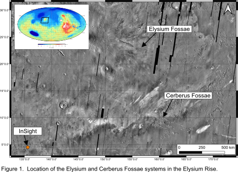
2. Cross-section balancing and geometry of the intrusions
The studied grabens are between 30-140 km long, and between 0.6-2.5 km wide, being therefore similar in length to the structures at Elysium Fossae, but significantly wider. 12 orthogonal cross sections to the grabens were constructed across the same number of structures. Topographic profiles were constructed using the PEDR dataset of the MOLA instrument.
Section balancing is achieved by calculating the lost area within the graben and estimating the heave of the graben-bounding faults. Graben area is calculated under basic assumptions; that the faults have angles of 60º, that the maximum depth observed in the graben is the actual depth, and that the undisturbed topography away from the faults represents the regional elevation. This allows to obtain a proxy of the depth of the upper dike tip and of dike width, which is assumed as equivalent to the sum of fault heaves.
Applying this methodology to the Cerberus grabens yields results which are consistent with previous work in Elysium, with theoretical considerations of dike-induced grabens, and with numerical experiments. However, the estimated dike widths at Cerberus are between 100-800 m, much larger than in any other Martian or terrestrial example. Despite this greater dimensions, width-length scaling relationships for the inferred Cerberus dikes are observed to be broadly consistent with sublinear scaling (Figure 2), which is characteristic of fluid-induced cracks [4]. Therefore, their geometry is consistent with that of giant dikes.
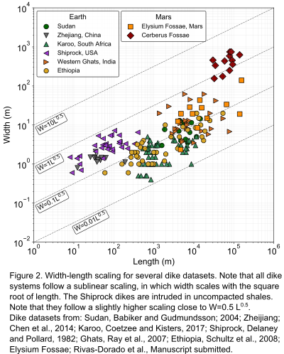
The much larger widths of the Cerberus dikes are an interesting feature. Martian dikes are expected to be of greater size relative to terrestrial dikes [5]. However, the Cerberus dikes are roughly one order of magnitude above the average width of the Elysium dikes. An observation made in several terrestrial datasets is that dikes intruded in uncompacted or fractured rocks tend to have greater widths than those intruded in intact rock [6]. We used simple principles of Linear Elastic Fracture Mechanics (LEFM), to explore the possibility that the Cerberus dike hint to a, at least locally, fractured crust.
3. Stress factors and their implications for the state of the crust
The stress intensity (Ki) factor is a measure of the stress required at the tip of a geological discontinuity to induce deformation. In the case of mode-I discontinuities (dikes, veins, and joints), the corresponding stress intensity factor is KI, and must be above a critical value (KIc) for propagation to occur. The fundamental expression of KI is [7]:
(1) KI=Yσe√(πa)
where Y is a geometric parameter dependant on fracture geometry, σe is excess pressure, and a is the fracture’s half length. However, if the opening of an individual fracture and the mechanical properties of the host rock are known, KI can also be calculated with the compact formula [8]:
(2) KI= [E/4(1-ν2)] Dmax √(π/a)
Where E is Young’s Modulus, υ is Poisson’s ratio, and Dmax is maximum opening. (1) shows clearly that KI depends mainly on fracture geometry and driving pressure. Therefore, cracks with similar geometry and formed under similar conditions should have similar values of KI. Previously calculated KI values at Elysium Fossae, which assumed intact basalts as the host rock, are between 3-15 GPa m1/2. These yielded reasonable estimations of excess pressures, in line with overpressures in Martian magmatic chambers. Since both Elysium and Cerberus Fossae belong to the same volcanic system, the dikes at Cerberus would be expected to reflect similar ranges of stress factors and excess pressures. However, similar KI values can only be obtained here if the properties of a fractured rock mass are presumed. Under this assumption, the inferred Cerberus dikes yield stress factors, calculated with (2), which are consistent with the theoretical factors of elliptical cracks formed at excess pressures of around 25 MPa (Figure 3).
4. Conclusions
Cross-section balancing applied in the Cerberus Fossae grabens yields values that describe an underlying dike system consistent with previous work and with the expected geometry of fluid-induced cracks. Furthermore, for these dikes to be emplaced under similar conditions to the neighbouring dike systems of Elysium Fossae, the host rock at Cerberus needs to have properties akin to those of a weak rock mass. This would provide an explanation for the gigantic dimensions of the dikes, and would likely have implications for the behaviour of the possibly seismogenic faults at depth.
References
[1] Giardini, D., et al., 2020. The Seismicity of Mars. Nat. Geosci. 13, 205–212. https://doi.org/10.1038/s41561-020-0539-8.
[2] Plescia, J.B., 2003. Cerberus Fossae, Elysium, Mars: A source for lava and water. Icarus 164, 79–95. https://doi.org/10.1016/S0019-1035(03)00139-8.
[3] Rivas-Dorado, S., et al. Submitted manuscript.
[4] Olson, J.E.: Sublinear scaling of fracture aperture versus length: An exception or the rule?, Journal of Geophysical Research, Vol. 108, NO.108, 2003.
[5] Wilson, L., Parfitt, E., 1990. Widths of dikes on Earth and Mars, LPI Technical Report 90-06. Houston.
[6] Delaney, P.T., Pollard, D.D., 1981. Deformation of Host Rocks and Flow of Magma during Growth of Minette Dikes and Breccia-bearing Intrusions near Ship Rock, New Mexico. USGS Prof. Pap. 1202 69.
[7] Lawn, B.R., Wilshaw, T.R.: Fracture of Brittle Solids, 204 pp., Cambridge Univ. Press, 1975.
[8] Schultz, R.A., 2019. Geologic Fracture Mechanics. Cambridge University Press, Cambridge. https://doi.org/https://doi.org/10.1017/9781316996737.
How to cite: Rivas-Dorado, S., Ruiz, J., and Romeo, I.: Evidence of dikes intruding a fractured crust beneath Cerberus Fossae, Europlanet Science Congress 2020, online, 21 Sep–9 Oct 2020, EPSC2020-642, https://doi.org/10.5194/epsc2020-642, 2020.
Abstract
Pit chains commonly occur along a bounding fault, allowing to infer a genetic relationship between grabens and pits. In this work we propose a comprehensive model for the formation of pit chains , the complex sequence of rift system and troughs in Noctis Labyrinthus. Like other previous authors, we confirm that a volcano-tectonic activity is the main process controlling the generation of such interesting and intricate structures in the studied area. We analyzed the geometrical properties and the maximum displacement as a function of fault length and cumulative frequency of fault length distribution for 499 mapped faults, which reveal the host lithology of the faults and the arrangement of rocks in of the crust and the lithosphere.
We finally suggest a model where a relative sequence of events responsible for the formation and development of the scalloped network of troughs in Noctis Labyrinthus (Mège et al.,2003).In this model, the magma propagates from depth to the surface by exploiting a network of interconnected fractures, and as a consequence, this magma inflation generates the formation of dike-induced grabens and pit chain on the surface.
Introduction
Noctis Labyrinthus is one of the enigmatic area in the surface of Mars.This area is made up by a complex inter-connected network of canyons and branched extensional faults and grabens Fig.1.These particular features of unknown origin, make Noctis Labyrinthus an interesting target to understand the possible factors that control the formation of these complex grid of troughs and infer the possible fault system evolution. We performed a detailed qualitative and quantitative study of these faults system through the study of their geometrical properties and surface morphology in order to understand their mechanical evolution and variations over different scales of length, the mechanisms of growth and the related stress field. We measured the maximum displacement as a function of faults length. The Dmax/L diagram provides slightly different results according to the fault type, since this ratio change from normal, thrust, and strike slip faults, so it provides information about the possible nature of the faults in the selected area (Seog Kim et al., 2005). The cumulative frequency plot Fig.3 was used to infer the scaling law of the fault system and faults growth, determine the lithology of the faulted rocks, the arrangement of materials in the subsurface and also the vertical confinement of faults vs. penetration of the brittle crust (Sornette.,2009; Torabi and Berg., 2011;Sornette et al., 1993; Cowie et al., 1991).

Fig.1.Surface interconnection between faults and pit chains, which follow a linear trend. Faults sizes and colors are labeled on the graph.
1. Data and methods
In our work, as a basemap, we used two orthoimages H3210_0000 and H3221_0000 from High Resolution Stereo Camera (HRSC) on board Mars Express, bearing a resolution of 12.5 m/pixel and for the surface topography, we utilized an individual Digital Elevation Model (DEM) from Mars Orbiter Laser Altimeter (MOLA) on board Mars Global Surveyor, with resolution of ~460 m/pixel. With these data sets, we made all morphometric measurements required for characterizing the faults and the grabens systems, analyzing faults distribution using rose diagrams, measuring faults lengths and the maximum vertical displacement of faults population and carry out a DMax Vs. L diagram and a cumulative frequency plot by input data in Origin software. Afterward, we studied the relationship of those fractures in terms of the formation and evolution of Pit chains and troughs.
2. Discussion and Conclusion
Noctis Labyrinhus is a framework of intricate rifts systems and branched faults, that have coalesced together to form an interconnected topography characterized by large troughs and canyons, driven by an invariant extensional stress field. Fault grow and develop at the same way but at different scales (Schultz et al., 2000; Turabi and Berg., 2011).
Crustal-Scale linkage in localized faulting zone is responsible for the formation of rift segment border by a pre-existing fracture (Soliva and Schultz., 2008). So far, only a few locations on Mars, where the DMax/L relationship has been measured. In our work, the nonlinear distribution in the Fig.2 might be explained by the presence of small size fractures, with different depths, which could be one of reasons that affect the large distribution of measurements in the Displacement-Length diagram (Turabi and Berg., 2011), or alternatively, it could be linked to the brittle crust thickness that control the displacement and the length of faults as in the terrestrial analogues faults systems (Soliva and Schultz., 2008; Schultz and Fossen.,2002; Soliva et al., 2005; Comie., 1998).

Fig.2. DMax /L diagram of faults studied in this work, shows a large scattering of values. The different DMax /L limits are plotted in various lines with different colors. Topographic offsets was measured along single MOLA tracks.
The cumulative frequency Vs. Length of fault population values grows in exponential fit Fig.3 of size distribution, mainly reflecting the presence of layered sequence of massive basalt (R.Soliva and R.Schultz., 2008).

Fig.3.The cumulative size distribution of the fault length population with Exponential and Power Law fits. On the diagram, the Exponential function fits the most with the main trend.
Furthermore,We classified pit chains as a morphological features of volcanic collapse generated by pressure drop above dikes (Mège and Masson., 1996; Liu and wilson., 1998; Scott et al., 2000; Mège and Masson., 1996; Wilson and Head., 2002; Ernst et al., 2001; Mège et al.,2003).Dikes play an important role to connect the surface to the magmatic source. The magma chamber at depth continuously generate flow that will be transported later to the upper levels through the dikes (Mège et al.,2003). This procedure will produce a stress in the dike tip, followed by deflation causing the collapsing of the surface, where there is a graben already formed. This sequence of events is responsible for the generation of the pit chain.We are suggesting a model based on a coupled physical processes of an early extension, visible on the surface by a forked grid of faults and grabens and a magma plumbing.
Acknowledgements
This research has been supported by European Union’s Horizon 2020 under grant agreement N° 776276-PLANMAP.
How to cite: El Yazidi, M., Pozzobon, R., Penasa, L., Debei, S., and Massironi, M.: The study of the relationship between Pit chains and grabens and their role in the formation of Rift systems and Troughs in Noctis Labyrinthus, Europlanet Science Congress 2020, online, 21 Sep–9 Oct 2020, EPSC2020-1069, https://doi.org/10.5194/epsc2020-1069, 2020.
Krupac crater in Sirenum Fossae, Mars: Understanding fresh impact cratering processes
S. Vijayan, Harish and Bhalamurugan Sivaraman
Planetary Science Division, Physical Research Laboratory, Ahmedabad, India.
vijayansiva@gmail.com
Introduction: The formation and evolution of impact craters can be studied using the fresh craters with distinguishable rays on Mars. Fresh craters with rays on Mars provide ample evidence for their preservation of impact event, records the post-impact modification, which reveals the recent geological activities. This fresh preserved ejecta is used as a chronological marker to understand the Amazonian geological activities. Apart from this, the fresh craters are also used to explore the target materials, which got exposed and excavated by the impacts. Apart from rays, such craters are potential targets for gullies, fan-like deposits, RSL, boulders, rim alteration, etc. Earlier studies [1, 2] identified rayed craters with few km diameter and inferred that they preserved the recent geologic records and could be possible events for the Martian meteorite source. Also, such fresh craters can be used as a potential analogy for the experimental impact cratering. In this initial study, we report geological records preserved within the Krupac crater (~1 km diameter) with fresh ejecta preserved around it (Figure 1a). This crater is located on the eastern side of the Eridania basin [3] in the Sirenum Fossae region. Krupac crater is located within the Simois Colles region. This part is geologically diverse and appeared to contain isolated paleolakes [3]. The rim of the Simois Colles region contains Al-Phyllosilicates [3], and some of the floor deposits indicates the presence of Olivine. The Krupac crater target material is thus a mixture of mafic and hydrated minerals.

Figure 1. a) Krupa crater and its fresh ejecta from HiRISE image (ESP_059256_1415), b) HiRISE colour image (ESP_059256_1415) shows the undissected rim, RSL, and unaltered rim on southern side.
Results and Discussion: The fresh ejecta is observed to span up to six crater radii, and it is not as far spread as other bright rayed crater reported by [2]. This ~1 km diameter craters ejecta spread is almost isotropic, but few rays are extended far than this 6 crater radius. Such discontinuous ejecta is challenging to distinguish due to their faded nature. The crater interior hosts gullies, large alcoves on the northern wall, which are possibly formed due to the pole facing activities within the crater. The equator facing wall of the crater completely lacks any such features and retains its pristine rim. These incised gully activities are one of the recent activities within the crater. The incised alcoves on the northern wall altered the rim of this fresh crater significantly. This incising alcove suggests that the rim wall is getting altered or extended due to this. This incision is varying around the crater and this helps to decipher about the differential erosion occurring within the crater. On average this incision is ~20 m from the pristine crater rim wall on the northern side (Figure 1b). This rim incision due to the alcove is altering the crater significantly [4], and some of the undissected rim is also present on the northern side as patches. This is the evidence for the differential weathering over the crater wall. Thus, such fresh crater rim incision reveals how crater rim erodes/alters over time.
On the crater rim, Recurring Slope Linea (RSL) are observed in large numbers [5,6,7] (Figure 1b). A small notable variation in the RSL length within HiRISE temporal images is observed. They are observed on top of the rim and over the terraced-like wall deposits within the crater. Mineralogically analysis using the CRISM suggests a noisy spectral signature over the crater region. A first degree polynomial fit for the median ratioed CRISM spectra extracted around the crater suggest presence of Phyllosilicate/clay signature. The indistinct spectra (Figure 2a) also shows a clay mixed carbonate-like signature. The carbonate absorption bands also occur/overlap with phyllosilicate Mg/Fe-OH hydroxyl bands [8]. It is unclear due to indistinguishable absorption; the detected minerals represent the exact surface mineralogy. Further analysis is needed to decipher their exact hydrated nature. There is no notable spectral signature from the RSL locations. The host surface of this crater holds the deposits of Fe/Me-phyllosilicates with light-toned deposits [3]. This Krupac crater is located on the sloped surface, which suggests that the earlier transported sediments were the host for this crater. Thus, the heterogeneous target for this Krupac crater and their younger nature is one good analogy for experimental cratering.

Figure 2. a) CRISM median ratioed spectra with notable absorption around ~2.29-2.31 µm and ~2.5 µm, b) crater size-frequency distribution estimated age for Krupac crater is ~4 Ma.
The Crater size-frequency distribution for the Krupac crater suggests a younger age of ~4 Ma (Figure 2b). This young Late Amazonian age, along with the preserved ejecta ray suggest that this Krupac crater preserved the recent geological activities and exposed the Noachian aged target materials. The presence of RSL, aqueous minerals may indicate that such fresh craters could be potential target for bio-signatures studies [6]. Overall, the Krupac crater is one of the well-preserved craters on Mars to decipher 1) rim-incision on the pole/equator facing walls, 2) RSL activities over the crater wall, 3) exposure of subsurface hydrated target materials and infer their heterogeneous mixtures, and 4) the well-preserved crater with ejecta and boulders can be used for comparing laboratory-based impact cratering experiments.
References: [1] McEwen A. S. et al., Icarus, 2005 [2] Tornabene et al., JGRPlanets, 2006 [3] Solmaz Adeli., et al; JGRPlanets, 2015 [4] Stucky de Quay et al., JGR Planets, 2019, [5] Chojnacki et al, JGRPlanets, 2016, [6] McEwen. A. S. 2018, LPSC2018. [7] Bishop, J. L. et al., LPSC 2019. [8] Brown, A. J. et al., JGRPlanets, 2020.
How to cite: Vijayan, S., Harish, N., and Sivaraman, B.: Krupac crater in Sirenum Fossae, Mars: Understanding fresh impact cratering processes, Europlanet Science Congress 2020, online, 21 Sep–9 Oct 2020, EPSC2020-1075, https://doi.org/10.5194/epsc2020-1075, 2020.
Introduction
The topographic correction of satellite images has to be applied to both disentangle albedo features from illumination effects induced by local topography and to perform thorough spectrophotometric analyses of planetary surfaces. This abstract focuses on the modelling and removal of surface brightness variations induced by topography, referred as topographic shading, from high-resolution visible images of Mars. We validate our method and report scientific applications to both single and multi-band datasets by analyzing High Resolution Imaging Science Experiment (HiRISE, [1]) colour observations of Martian recurring slope lineae (RSL, [2] ) and dust devil tracks [3] and Colour and Surface Science Imaging System (CaSSIS,[4]) panchromatic observations.
Data and methods
We initially apply the topographic correction (i.e. modeling and removal of topographic shading) to HiRISE images of Tivat Crater (-45.9°N, 9.5°E, Fig. 1A), Mars. This site hosts RSL (i.e. dark linear features that appear in warm season, fade in cold ones and recur annually) and dust-devil tracks (i.e. low-albedo tracks left by turbulent whirlwinds). Both features show a different albedo from nearby surfaces, representing an interesting scientific application of our method. In addition, relative photometry of Tivat crater’s RSL with respect to a “normalization” region having their same illumination and observation conditions (Fig. 2A) was recently published [5], offering us a benchmark for validating our method. All available HiRISE orthoimages of Tivat crater were radiometrically calibrated and atmospherically corrected with the dark pixel method, as in [5]. For each image, we followed the approach of [6] to compute local incidence and emission angle maps from the HiRISE DTM of the selected site. These maps were used to correct the image through the Lambert [6], Lommel-Seeliger [7], Akimov [8] and Minnaert [9] disk functions. The one returning the most uniform brightness values was selected for the photometric analysis. An example correction is shown in Fig. (1). We repeated the relative albedo analysis of [5] using both the original and corrected images. While with original images, affected by topographic shading, we obtain different results, our measurements on the topographically corrected images (Fig. 2B) and the derived time evolution of the RSL and nearby regions relative albedo (Fig. 2C) are consistent with [5], hence validating our method.
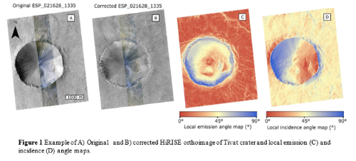
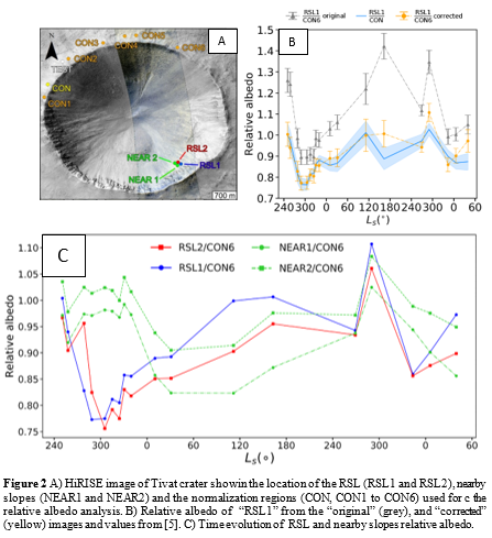
Results: HiRISE and CaSSIS case studies
Multi-band photometry of RSL. We extended our method to the BG and NIR bands of HiRISE color orthoimages of Tivat crater. Our measurements in Fig. (3C) suggest that RSL are darker than nearby slopes but have the same colours within measurement uncertainties, in agreement with [2]. The same result also holds between RSL and the dust-devil tracks, hence possibly suggesting that RSL could be dust-removed features too.
Topographic correction of CaSSIS panchromatic images. We corrected a CaSSIS panchromatic image depicting the north-eastern part of the Ascraeus Mons summit caldera complex (11.2°N, 255.9°E, Fig. 4C). Featuring a rich variety of slope orientations, this location represents a challenge for our method. The stereo observation of the site allowed the production of both DTM and orthoimages through the 3DPD photogrammetric pipeline [11]. These products, available through the Cassis DTM Repository [12], along with the computed local incidence and emission angle maps and the topographically corrected image are shown in Figure (4).
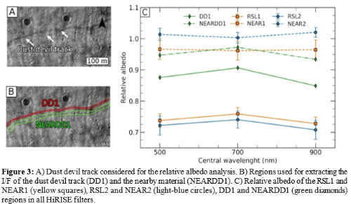
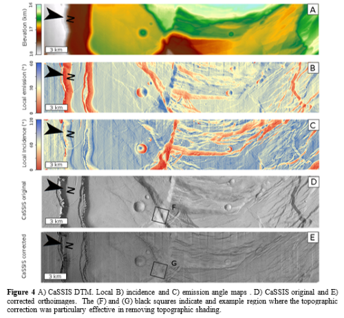
Conclusions
We presented and validated a method for removing topographic shading from HiRISE and CaSSIS images. We showed example applications by correcting HiRISE color datasets and a CaSSIS panchromatic image. The corrected images (Fig. 1,4) present a more uniform surface brightness, consistent with the removal of topographic shading. Corrected HiRISE color observation of RSL and dust-devil tracks allowed to investigate and compare the photometric properties of these features in all the HiRISE bands. The full methodology and scientific analyses of these datasets will be presented and discussed at the conference.
Acknowledgments: The authors wish to thank the spacecraft and instrument engineering teams for the successful completion of the instrument. CaSSIS is a project of the University of Bern and funded through the Swiss Space Office via ESA’s PRODEX programme. The instrument hardware development was also supported by the Italian Space Agency (ASI) (ASI – INAF agreement no. I/018/12/0), INAF/Astronomical Observatory of Padova, and the Space Research Center (CBK) in Warsaw. Support from SGF (Budapest), the University of Arizona (Lunar and Planetary Lab.) and NASA are also gratefully acknowledged. The study has been supported by the Italian Space Agency (ASI-INAF agreement no. 525 2017-03-17).
References
[1] A. S. McEwen et al. (2007), JGR:Planets
[2] A. S. McEwen et al. (2011), Science
[3] D. Reiss et al. (2016), SSR
[4] N. Thomas et al. (2017), SSR
[5] E. I. Schaefer et al. (2019), Icarus, 317,621–648
[6] B. Hapke, Theory of reflectance and emittance spectroscopy,1993
[7] M. B. Fairbairn (2005), \jrasc,99,3,92
[8] S. E. Schröder et al. (2013), PSS,85,198–213
[9] M. Minnaert (1941),Astrophys. J., 93,403–410
[10] P. K. Byrne et al. (2012), JGR:Planets
[11] E. Simioni et al. (2017), Int. Arch. Photogramm. Remote Sens. Spat. Inf. Sci.,vol. XLII-3/W1,133–139
[12] G. Cremonese and C. Re (2018), EPSC2018-1236.
How to cite: Munaretto, G., Pajola, M., Lucchetti, A., Re, C., Cremonese, G., Simioni, E., and Cambianica, P.: Topographic correction of HiRISE and CaSSIS images: validation and application to multi-band photometry of Martian recurring slope lineae, Europlanet Science Congress 2020, online, 21 Sep–9 Oct 2020, EPSC2020-328, https://doi.org/10.5194/epsc2020-328, 2020.
Introduction: Bright slope streaks are enigmatic surface features of increased albedo found on Martian slopes in low thermal inertia regions [1, 2]. These elongated features are thought to form as the more common dark slope streaks [3, 4] gradually fade or brighten with time [5]. In fact, in a few rare cases slope streaks have been observed to have bright and dark sections [1, 5, 6], which could be taken as evidence of this transition. The fading rate of dark slope streaks has been shown to be around 40 years [7] but the contrast reversal rate is unknown. Several hypotheses attempt to explain the origin of dark slope streaks: Dry-based models encompass formation through dust mass wasting, avalanching or granular flows [1, 6, 8]; and aqueous models cite subsurface aquifers as sources, lubricated dust flows and ground staining from saline fluids [9-13]. Various properties of dark slope streak populations were studied in detail to address their origin [14-16]. However, little is known about the physical parameters that would affect their photometry, e.g., surface texture, roughness and grain size. Here, we address this issue by acquiring multi-angular observations of bright slope streaks using the Colour and Stereo Surface Imaging System (CaSSIS) [17] onboard the ExoMars Trace Gas Orbiter (TGO). When necessary and available, we complement these observations with higher-resolution images of our study sites taken by the Mars Reconnaissance Orbiter’s (MRO) High Resolution Imaging Science Experiment (HiRISE). To obtain regional context for our observations, we used a global Context Camera (CTX) mosaic [18] to grid-map the locations of bright slope streaks in the Arabia Terra region [19].
Results: We surveyed the distribution of bright slope streaks in Arabia Terra using a grid map divided into ~16,000 hexagonal facets, each 20 km in diameter, and each qualitatively surveyed. Additionally, we documented ~30 locations of partially dark-bright slope streaks. We targeted one such peculiar case (first observed by the Mars Orbiter Camera (MOC) [1]) with CaSSIS and HiRISE (Fig. 1). This example features a bright apex that begins to darken towards the middle, and at the distal end appears indistinguishable from a dark slope streak. This same albedo reversal is visible under various lighting geometries (23°-86° incidence). We used these multi angular observations as the basis for photometric measurements of this slope streak, which are seen in Fig 2. We measured I/F values (detected irradiance (I) over the solar irradiance at zero incidence (F), such that I/F = 1 for a normally illuminated, perfectly diffuse reflector) of dark and bright slope streak regions-of-interest (ROIs), and ratioed them over the ROIs of the surrounding surface. This method avoids the reflectance dependency on local slope. Fig. 2 indicates that the dark (black squares) and the bright (red circles) part of the slope streak is up to 4.5% darker and 3.5% brighter respectively. It also appears that between years 2009-2014 (three HiRISE observations) the dark slope streak ROI is darker than in the three CaSSIS observations taken in 2020.
Discussion: In the past, the contrast reversal of slope streaks was attributed to either physical fading (coverage by atmospheric dust fallout) [5] or viewing geometry effects [6]. Loose snow avalanches on Earth were suggested as a possible analogous process where the latter effect occurs [e.g. 1, 6]. Interestingly, many dark, bright and dark-bright streaks are frequently found on the same slope, which suggests that their albedo is independent of viewing geometry. This is supported by the multiple observations seen in Fig. 1. Reflective behavior appears to be independent of illumination geometry, i.e. the slope streak exhibits the same contrast reversal in all observations. Further, our quantitative photometric measurements (Fig. 2) support this finding. The ratio of the dark ROI and the surroundings within 3 HiRISE observations is almost linear, but the earlier HiRISE image exhibits a higher ratio. The later (2020) 3 CaSSIS images of the dark ROI ratios illustrate a more faded streak. This fading could be a result of atmospheric dust fallout (e.g. dust storm in MY34), but this would not explain the bright ROI behavior. Another hypothesis is that the fading is related to gravity-controlled processes. Particles at the top of the streak might be more easily churned by wind and transported downwards by mass wasting. To investigate these two hypotheses, we will use a CaSSIS-based Digital Terrain Model (DTM) to accurately measure slopes and constrain their photometric effects, and a reflectance model based on Hapke theory [20] to simulate the difference in spectral reflectance between regolith with a variety of grain size distributions.
References: [1] Sullivan R. et al. (2001) JGR, 106, 23607-23633. [2] Schorghofer N. et al. (2002) GRL, 29, 2126. [3] Morris, E. C. (1984) JGR, 87, 1164–1178. [4] Ferguson H. M. & Lucchitta B. K. (1984) NASA Tech. Memo. 86246, 188-190. [5] Schorghofer N. et al. (2007) Icarus, 191, 132-140.[6] Baratoux D. et al. (2006) Icarus, 183, 30-45. [7] Bergonio J. R. et al. (2013) Icarus, 225, 194-199. [8] Chuang F. C. et al. (2007) GRL, 34(L20204). [9] Ferris J. C. et al. (2002), GRL, 29. [10] Miyamoto H. et al. (2004) JGR, 109, E06008. [11] Kreslavsky M. A. and Head J. W. (2009) Icarus, 201, 517-527. [12] Head J. W. et al. (2007) AGU Fall Abstracts, (#P22A-08). [13] Bhardwaj A. et al. (2019) Rev. Geophys., 57, 48-77. [14] Schorghofer N. and King C. M. (2011) Icarus, 216, 159-168. [15] Brusnikin E. S. et al. (2016) Icarus, 278, 52-61. [16] Mushkin A. et al (2010), GRL, 37, L22201. [17] Thomas N. et al. (2017), Space Sci. Rev, 212, 1897-1944. [18] Dickson J. L. et al. (2018), LPSC XLIX, Abstract #2083. [19] Ramsdale J. D. et al. (2017) PSS, 140, 49-61. [20] Hapke, B., 2012. Theory of Reflectance and Emittance Spectroscopy, 2nd ed. Cambridge University Press.
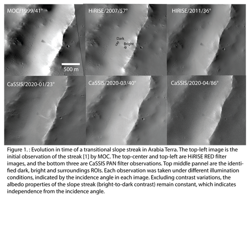

How to cite: Valantinas, A., Becerra, P., Tornabene, L. L., Pommerol, A., Hauber, E., Thomas, N., McEwen, A., and Cremonese, G.: Multi-angular Observations of Martian Bright Slope Streaks, Europlanet Science Congress 2020, online, 21 Sep–9 Oct 2020, EPSC2020-1062, https://doi.org/10.5194/epsc2020-1062, 2020.
Introduction: This study focuses on four unusual landslides located inside a 25 km diameter impact crater located in Nilosyrtis Mensae (Fig.1). Our initial study revealed that one of these landslides bears close similarity to a mudslide on Earth [1]. We performed a detailed morphological analysis and a comparison with terrestrial analogues to better understand their formation mechanism. We also consider the possible role of volatiles in their formation.
Approach: We used the Colour and Stereo Surface Imaging System (CaSSIS) [2] and ConTeXt imager (CTX) with a resolution of 6 m/pix and 5 m/pix, respectively, to carry out a regional study, while the High Resolution Imaging Science Experiment (HiRISE) images with a resolution of 25-50 cm/pix were used to carry out a detailed study of the landslides. We also used the HiRISE data to make Digital Elevation Models (DEMs) at 2 m/pix produced using the standard workflow in ISIS and SocetSet [3].
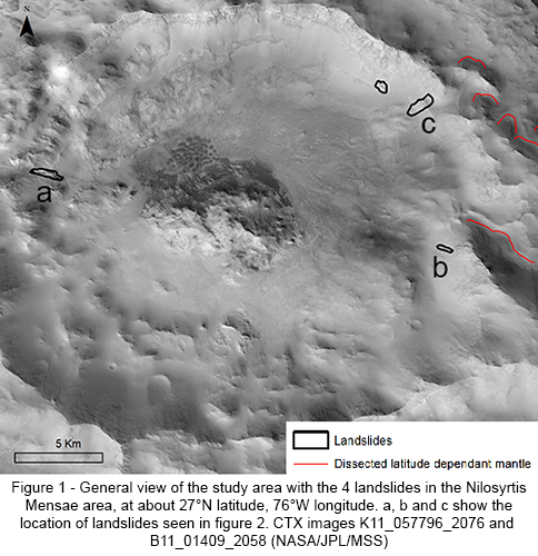
Morphological analysis results: The host crater has a rounded rim and highly degraded ejecta suggesting a Hesperian to Early Amazonian age. The crater shows some evidence of dissected latitude dependant mantle on pole-facing slopes on the outer crater walls (Fig.1) –
this is an ice-rich deposit which is thought to date to a few tens of Ma [4]. There are also ~200 well-preserved rockfall tracks on the eastern crater wall, indicating that the interior of the crater has had episodes of recent destabilization during the late Amazonian. The landslides have the following features in common: (1) a sliding surface with an angle between 20 and 25°; (2) an irregular, well-defined erosion zone; (3) compression ridges on the deposit; (4) a lobate deposit margin; and (5) lateral levees on 3 out of the 4 landslides with a thickness between 5 and 25 meters. In addition, on two of the four landslides, there are secondary failure scars within the main landslide deposit, suggesting reactivation, as shown in in Figure 3a. In addition, the overall morphology of these four landslides suggests a late Amazonian formation-age, based on their pristine appearance and the absence of impact craters on the deposit. The broadly similar ages of the landslides and the degraded latitude dependent mantle suggests a potential link.
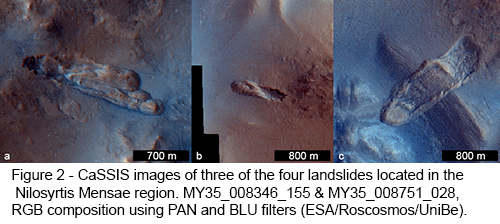
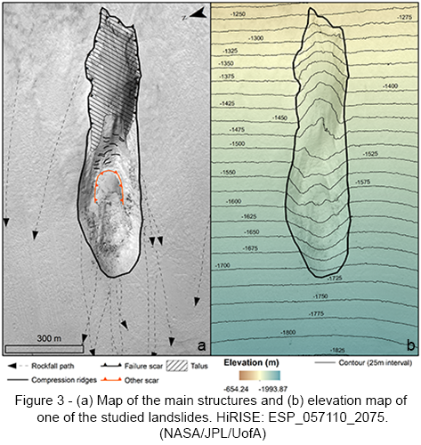
Terrestrial comparison: We conducted a morphological and rheological comparison with terrestrial analogues to better understand the flow dynamics of these martian landslides. We found that these landslides are most comparable with terrestrial earthflows, because they also: (1) occur on low surface slopes, (2) have lateral levees (3) have high relief lobate flow fronts and (4) possess similar material yield strength values around 100 kPa [5]. We estimated the yield strength of our martian landslides to be 1-100 kPa by using the cross-profile morphology of the flows as described in [6].
Conclusions: (1) We see numerous rockfall tracks showing the presence of recent instabilities in this region. (2) The observation of dissected latitude dependant mantle reveals ice has recently been present in the ground in this region. (3) The comparison that we made between the martian landslides and terrestrial analogues reveals similarity with earthflows in terms of morphology and rheology. (4) Liquid water is key to allowing earthflows to move on Earth, and the dissected latitude dependant mantle near the impact crater reveals the presence of ice in the past. We therefore propose that ice could have been involved in the formation of these landslides.
Acknowledgements: This thesis is funded by a ministerial grant. We are grateful for the support of the Programme National de Planétologie and the French Space Agency CNES. The authors thank the spacecraft and instrument engineering teams for the successful completion and operation of CaSSIS. CaSSIS is a project of the University of Bern funded through the Swiss Space Office via ESA's PRODEX program. The instrument hardware development was also supported by the Italian Space Agency (ASI) (ASI-INAF agreement no. I/018/12/0), INAF/ Astronomical Observatory of Padova, and the Space Research Center (CBK) in Warsaw. Support from SGF (Budapest), the University of Arizona (LPL) and NASA are also gratefully acknowledged.
References: [1] Guimpier et al. (2020) PSS, submitted. [2] N. Thomas et al. (2017) Space Sci. Rev., 212, 1897–1944. [3] R.L. Kirk et al. (2008) JGR, 113. [4] R.E. Milliken et al. (2003) JGR, 108, E6. [5] A.L. Nereson and N.J. Finnegan (2015) AGU Fall Meet. Abstr., EP41C-0943. [6] D.M. Pyle and J.R. Elliott (2006) Geosphere, 2, 253–268.
How to cite: Guimpier, A., Conway, S., and Mangold, N.: Atypical landslides in the Nilosyrtis region of Mars, Europlanet Science Congress 2020, online, 21 Sep–9 Oct 2020, EPSC2020-746, https://doi.org/10.5194/epsc2020-746, 2020.
Digital Elevation Models (DEM) are widely used tools in planetary sciences. Geometric parameters such as pixel orientations and local slopes can be derived from these DEM. However, as any data, DEM have a limited precision (i.e. errors), which yields to the propagation of errors on geometric parameters. Assessing local slopes is necessary for many morphological studies: then, how do the DEM vertical errors propagate on the slope values? To answer to this question, we develop a simple and fast numerical method based on the addition of noise on synthetic DEM. We evaluate the different components of slope errors to define the relationship between input DEM noise and output slope errors. Results can be used as first order estimations to discuss slope maps precision.
How to cite: Millot, C., Quantin-Nataf, C., and Leyrat, C.: Assessing slope precision from numerical propagation of DEM (Digital Elevation Model) vertical errors, Europlanet Science Congress 2020, online, 21 Sep–9 Oct 2020, EPSC2020-881, https://doi.org/10.5194/epsc2020-881, 2020.
Please decide on your access
Please use the buttons below to download the presentation materials or to visit the external website where the presentation is linked. Regarding the external link, please note that Copernicus Meetings cannot accept any liability for the content and the website you will visit.
Forward to presentation link
You are going to open an external link to the presentation as indicated by the authors. Copernicus Meetings cannot accept any liability for the content and the website you will visit.
We are sorry, but presentations are only available for users who registered for the conference. Thank you.