OPS4 | The Mysterious Saturn System

OPS4

The Mysterious Saturn System
Co-organized by MITM
Convener: Conor Nixon | Co-conveners: Mauro Ciarniello, Alice Lucchetti, Nadine Nettelmann
Orals
| Wed, 11 Sep, 10:30–12:00 (CEST)|Room Sun (Auditorium)
Posters
| Attendance Wed, 11 Sep, 14:30–16:00 (CEST) | Display Wed, 11 Sep, 08:30–19:00
Orals |
Wed, 10:30
Wed, 14:30
The Saturn system inspires awe with its brilliant bright rings, its diversity of moons from large to small, and the rapidly rotating planet itself with its polar hexagon and dramatic storm outbursts. The data from the Cassini-Huygens mission has aded more questions than answers, including whether the system has always looked this way, or it still rapidly evolving at recent times. This session welcomes submissions that address the many facets of the Saturn system, including those that seek to place it in the wider context of the solar system and exoplanetary systems.

Orals: Wed, 11 Sep | Room Sun (Auditorium)

Chairpersons: Conor Nixon, Mauro Ciarniello, Nadine Nettelmann
10:30–10:40
|
EPSC2024-31
|
On-site presentation
Ravit Helled

The formation history of giant planets inside and outside the Solar System remains unknown. We suggest that runaway gas accretion is initiated only at a mass of ∼100 M and that this mass corresponds to the transition to a gas giant, a planet whose composition is dominated by hydrogen and helium. Delayed runaway accretion (by a few million years) and having it occurring at higher masses is likely a result of an intermediate stage of efficient heavy-element accretion (at a rate of ∼10−5M yr−1) that provides sufficient energy to hinder rapid gas accretion. This may imply that Saturn has never reached the stage of runaway gas accretion and that it is a “failed giant planet”. The transition to a gas giant planet above Saturn’s mass naturally explains the differences between the bulk metallicities and internal structures of Jupiter and Saturn. The mass at which a planet transitions to a gas giant planet strongly depends on the exact formation history and birth environment of the planet, which are still not well constrained for our Solar System. In terms of giant exoplanets, the occurrence of runaway gas accretion at planetary masses greater than Saturn’s can explain the transitions in the mass-radius relations of observed exoplanets and the high metallicity of intermediate-mass exoplanets.

How to cite: Helled, R.: Is Saturn a failed gas giant?, Europlanet Science Congress 2024, Berlin, Germany, 8–13 Sep 2024, EPSC2024-31, https://doi.org/10.5194/epsc2024-31, 2024.

10:40–10:50
|
EPSC2024-181
|
ECP
|
On-site presentation
Saburo Howard, Simon Müller, and Ravit Helled

Studying the interiors of giant planets is important for understanding their origin. While accurate measurements of gravity field and seismology from Juno and Cassini teach us about the present-day internal structures of Jupiter and Saturn, further insights can be gained from simulating their evolution. Understanding the long-term thermal evolution of the giant planets is also critical to connect the planetary formation and the current-state structure of planets.

In Jupiter and Saturn, a phase separation between hydrogen and helium occurs, resulting in the formation of helium droplets which settle towards the deep interior. This phenomenon, also known as helium rain, can strongly affect their thermal evolution. Therefore, studying the evolution of Jupiter and Saturn, and giant planets in general, requires a good comprehension of the phase diagram of hydrogen and helium. However, the latter remains uncertain given the discrepancy between various theoretical calculations and experimental data.

I will present results of evolution models of Jupiter and Saturn with helium rain, using different phase diagrams. We find that a consistency between Jupiter's evolution and the Galileo measurement of its atmospheric helium abundance is achieved only if a shift in temperature in the existing phase diagrams is applied. We next use the shifted phase diagrams to model Saturn's evolution and find consistent solutions for both planets. We confirm that demixing in Jupiter is modest while in Saturn, the process of helium rain is significant. I will discuss the inferred structure of both planets, the inferred atmospheric helium content in Saturn and show the importance of equations of state and atmospheric models on evolution models. This analysis reveals key information on the interiors of giant planets and can also be used to constrain the phase diagram of hydrogen and helium.

How to cite: Howard, S., Müller, S., and Helled, R.: The evolution of Jupiter and Saturn with helium rain, Europlanet Science Congress 2024, Berlin, Germany, 8–13 Sep 2024, EPSC2024-181, https://doi.org/10.5194/epsc2024-181, 2024.

10:50–11:00
|
EPSC2024-234
|
ECP
|
On-site presentation
Peio Iñurrigarro Rodriguez, Alexander S. Medvedev, Ingo C. F. Müller-Wodarg, and Luke Moore

In the atmospheres of the Solar System planets, several kinds of atmospheric waves can be found. They are an important atmospheric phenomenon as, besides disturbing the atmosphere, they can also alter the mean structure and affect the general circulation [1]. Therefore, understanding their effects on the atmospheric dynamics is of paramount importance.

The thermospheres of the Giant Planets are hotter than what would be expected if solar heating were considered the only energy source. Historically, the few existing numerical models have had difficulties to reproduce the observed temperature structure at mid and low latitudes. It was long thought that waves propagating vertically might play an important role in determining the temperature by either heating the thermosphere [2, 3] or by weakening the intense high-latitude westward jets allowing the meridional transport of energy trapped in the polar regions [4, 5]. Recently, the detection of gravity waves in Saturn's thermosphere has been reported using data from Cassini INMS and UVIS occultation data [4, 5, 6].

The Saturn Thermosphere-Ionosphere Model (STIM) is the only 3D general circulation model published so far for Saturn's upper atmosphere [7, 8]. The model couples dynamically and chemically the thermosphere and the ionosphere. In this work, we have used the STIM model to perform high resolution numerical simulations of Saturn's thermosphere. They show the development of supersonic spiral gravity waves in the northern and southern auroral regions driven by the high latitude forcing produced by Joule heating and ion drag. We analyze the morphology and properties of these waves, their propagation and the forcing they impose on the mean flow. We also show simulations with forcing introduced at the bottom of the model to explore waves that can propagate through the thermosphere and their potential impact on the circulation.


References:

[1] Vallis. Atmospheric and Ocean Fluid Dynamics. Cambridge University Press, Cambridge, UK, 2006.

[2] Young et al. Gravity waves in Jupiter's thermosphere. Science, 276, 1997.

[3] O'Donoghue et al. Heating of Jupiter's upper atmosphere above the Great Red Spot. Nature, 536, 2016.

[4] Müller-Wodarg et al. Atmospheric Waves and Their Possible Effect on the Thermal Structure of Saturn's Thermosphere. Geophysical Research Letters, 46, 2019.

[5] Brown et al. Evidence for gravity waves in the thermosphere of Saturn and implications for global circulation. Geophysical Research Letters, 49, 2022.

[6] Brown et al. A pole-to-pole pressure-temperature map of Saturn's thermosphere from Cassini Grand Finale data. Nature Astronomy, 4, 2020.

[7] Müller-Wodarg et al. A global circulation model of Saturn's thermosphere. Icarus, 180, 2006.

[8] Müller-Wodarg et al. Magnetosphere-atmosphere coupling at Saturn: 1 – Response of thermosphere and ionosphere to steady state polar forcing. Icarus, 221, 2012.

How to cite: Iñurrigarro Rodriguez, P., Medvedev, A. S., Müller-Wodarg, I. C. F., and Moore, L.: Numerical simulations of atmospheric waves in Saturn's upper atmosphere, Europlanet Science Congress 2024, Berlin, Germany, 8–13 Sep 2024, EPSC2024-234, https://doi.org/10.5194/epsc2024-234, 2024.

11:00–11:10
|
EPSC2024-562
|
On-site presentation
Larry W. Esposito, Joshua P. Elliott, and E. Todd Bradley

Cassini observations of the micrometeoroid bombardment flux, ring mass and fractional pollution constrain the origin and history of Saturn’s rings. In the simplest model, the age of the rings can be estimated by assuming the rings are a closed system with constant bombardment at the current rate. However, the rings are not a closed system and Cassini spectroscopy is consistent with space weathering of the cosmic dust polluting the rings. The remote sensing of the rings shows a red slope, with higher pollution at the shortest wavelengths, consistent with reddening due to space weathering of atmosphereless bodies. If processes at the time of the micrometeorite impacts or subsequent chemical and physical weathering can degrade the original pollutants, this means that laboratory spectra are not appropriate to determine the total extrinsic material that has struck the rings over their lifetime. Laboratory results for irradiation of icy outer solar system analogues indicate oxidation of organics and other pollutants over time. It is now generally agreed that the radiolysis of ice by energetic ions, electrons and solar UV photons produces the oxygen, ozone and peroxide seen at many icy satellites. The porosity of ice provides sufficient space for chemical reactions and mobility. The ring particle surfaces are in addition continually gardened by particle collisions and meteoritic impacts. Because of the loss processes, the current fractional pollution provides only a lower limit on the total integrated pollution flux, and thus a lower limit for the ring age. Rosetta data on the dust composition and surface reflectivity of Comet 67P provide our starting point for the composition of the bombarding material: Two independent analyses of Cassini UVIS spectra of Saturn’s rings give fractional pollution in the outer B ring of 1.4 -3%. This provides a lower limit of 400 to 1600 million years for the most opaque parts of Saturn’s B ring, depending on whether we use the maximum or minimum values for the bombardment rate reported by Cassini CDA. This result shows Saturn’s rings may be as old as the planet Saturn itself, consistent with the estimates for the orbital evolution of ring moons Atlas and Epimetheus. The A and C rings may have formed more recently.


How to cite: Esposito, L. W., Elliott, J. P., and Bradley, E. T.: Space Weathering Provides a Lower Limit on the Age of Saturn’s Rings, Europlanet Science Congress 2024, Berlin, Germany, 8–13 Sep 2024, EPSC2024-562, https://doi.org/10.5194/epsc2024-562, 2024.

11:10–11:20
|
EPSC2024-920
|
On-site presentation
Sascha Kempf, Nicolas Altobelli, Jürgen Schmidt, Jeffrey Cuzzi, Paul Estrada, and Ralf Srama

One of the most exciting and controversial aspects of Saturn’s magnificent rings is that they may actually be a recent phenomenon in the solar system – forming long after the Earth, Saturn, and its moon. This possibility has been vigorously debated for nearly 40 years, since the Voyager flybys of Saturn. Over the years, the most powerful support for this hypothesis has turned out to be the puzzle of the rings’ nearly pure water ice composition – unique in the family of planetary rings – in spite of the constant hail of rocky-carbon meteoroids from outside the Saturn system. However, three major uncertainties have left the young-ring hypothesis unproven. Two of these have already been resolved by the Cassini mission: the amount of non-icy material currently in the rings, and the total ring mass. The third main constraint is the mass flux of non-icy meteoroids falling onto the rings. 

Measuring this mass flux was always a main science goal of the Cassini mission, and could only be achieved by the Cassini Cosmic Dust Analyzer instrument (CDA). In this talk we will report about the determination of the mass flux of non-icy material coming into the Saturn system, which completes the trifecta of constraints that are required to strongly support a youthful ring system [1]. The measurements present a thorough and detailed analysis of the series of unconnected individual particle detections by CDA over Cassini’s entire 13 year mission, converting these detections into the desired mass flux. The CDA detections determine the incident particle orbits, and they come (surprisingly) not from comets as expected, but mostly from Kuiper Belt Objects. This means that most of the particles have low speeds relative to Saturn and are strongly focused gravitationally, such that the flux at the rings is even larger than previously estimated. The derived mass flux implies a ring exposure time of less than 100 to 400 million years, which is in support of recent ring formation scenarios.

How to cite: Kempf, S., Altobelli, N., Schmidt, J., Cuzzi, J., Estrada, P., and Srama, R.: How old are Saturn’s rings?, Europlanet Science Congress 2024, Berlin, Germany, 8–13 Sep 2024, EPSC2024-920, https://doi.org/10.5194/epsc2024-920, 2024.

11:20–11:25
11:25–11:35
|
EPSC2024-981
|
On-site presentation
Carly Howett, Francis Nimmo, John Spencer, and Georgina Miles

Introduction: Enceladus’ activity is concentrated across its south polar terrain (SPT). The activity is concentrated along four fractures dubbed tiger stripes. Constraining the magnitude of the endogenic emission from this region has proved challenging, with estimates varying from 4.2 GW to 5.8 ± 1.9 GW and 15.8 ± 3.1 GW [1-3].

The reason for the discrepancy is due to how different studies disentangled the total (passive and endogenic) emission observed to isolate the endogenic component. In the 15.8 GW study estimated the magnitude of the passive emission through modelling and then subtracted from the total. The other studies instead assumed the low-temperature passive component was negligible by only considering only high-temperature (>80 K) endogenic emission across the SPT (5.8 GW), or just the tiger-stripes (4.2 GW).

So the different studies could not be contradicting each other. It’s feasible that the total endogenic emission is ~15.8 GW, but the tiger-stripe only emission is ~4.2 GW with the remaining ~11 GW coming from elsewhere. The most logical place for this extra emission is the region between the stripes, called interstitial (or funiscular) terrain. Thus, it is emission from this is the area that we focus upon in this work.

Data: Cassini Composite Infrared Spectrometer (CIRS) was highly sensitive to the peak power of their blackbody emission. CIRS was a Fourier transform spectrometer with three focal planes covering 10 to 1400 cm-1 (7.1 to 1000 μm) [4]. Focal plane 1 (FP1) covered 10 to 600 cm-1 (16.7 to 1000 μm) with a spatial reolution of 3.9 mrad, enabling it to be sensitive to thermal radiation above 40 K. This made FP1 particularly sensitive to the typical solar heated surface temperatures of the icy satellites and thus the focus of this work  . The specific CIRS FP1 data to be analysed is given in Table 1. An example of the CIRS coverage for a single scan is shown in Figure 2.

Cassini Orbit #

Date

# CIRS Observations

Spatial Resolution (km/pix)

61

03/12/2008

110

50-80

80

08/11/2008

59

3-23

90

10/31/2008

86

4-36

136

08/13/2010

219

11-29

228

12/19/2015

330

21-30

Table 1 – Details of the CIRS FP1 observations to be analysed. All encounters have a single FP1 scan except for Orbit 136 (6 scans) and Orbit 228 (4 scans).


Figure 1 – Footprints (shown by black elipses) of CIRS FP1 over Enceladus’ tiger stripe fractures taken during Orbit 136, first scan. The names of the tiger stripes are given. The solid line indicates the location of the center of the FP1 field of view, where the detector is most sensitive.

Method: Seasonal thermophysical models [5] are run over a range of expected thermophysical properties. The model accounts for Saturnshine and eclipses. The surface temperatures predicted by these models is then determined for each observation. Accounting for the Gaussian response of FP1 the surface temperatures are translated into a predicted radiance for each CIRS footprint and each set of thermophysical properties. These are then compared to the CIRS observed radiances to determine how well they agree.

Models that can fit the CIRS data close to, but not inside the SPT, imply they have thermophysical parameters consistent with those observed close to Enceladus’ SPT and thus provides a reasonable estimate of their value.

For these “good fit” models the difference between the observed and predicted radiances inside of the active regions can then be determined, to provide a constraint on the endogenic emission observed there.

Results: The analysis is ongoing, but here we present new results of a single scan taken during Orbit 136. The ground coverage of this scan was already shown in Figure 1. Model temperatures were obtained for albedos ranging from 0.7 to 0.9 in 0.25 increments, and between 5 and 100 MKS in 5 MKS increments below 50 MKS and 10 MKS increments above it. A subset of the model results are compared to the CIRS-derived temperatures in Figure 2.

The results show that the location of the tiger stripes is obvious in the FP1 data. The location of each stripe (indicated by vertical dotted line) coincides with a distinct increase in surface temperature ~10 K above the background. Between the fractures the temperature decreases to close to non-SPT temperatures. All model parameter sets are able to predict the CIRS observed temperatures at the start of the scan (outside the SPT). So none can be ruled out based on this study alone. However, it is obvious that the discrepancy between the predicted temperatures and those observed across the tiger stripes is highly model dependent.

Figure 2 – Model temperatures (red) compared with CIRS-derived surface temperatures (black). The distance given is from the start point (shown in Figure 1) following the FP1 ground track (shown by the solid line cutting through the ellipses in Figure 1). The dotted vertical lines indicate where an observation cuts across a fracture, from left to right these are: Damascus, Baghdad and Cairo. Note there is no model fit to the first six observations as they cover latitudes currently not modelled.

The difference between the model and observed temperatures is endogenic emission, so each model will predict a different endogenic emission. The range in endogenic emissions these models predict for this swath is between 0.02 and 0.45 MW km-2, with a mean value of 0.13 MW km-2. Assuming this mean value, and an SPT area of 13,500 km2 (the area polewards of 60  S) and such emission levels are constant across the active region then this implies the SPT could have a background endogenic emission of ~1.7 GW. We note this estimate is very preliminary and additional analysis will better constrain the thermophysical property regime and the spatial variation of the emission.

Acknowledgments: This work is funded through NASA CDAP 80NSSC19K0885.

References: [1] Spencer, J.R. et al., In Enceladus and the Icy Moons of Saturn, University of Arizona, 2018. [2] Spencer, J.R. et al., Science 311, 1401-1405, 2006. [3] Howett, C.J.A. et al., Journal of Geophysical Research 116, E03003, 2011. [4] Flasar, F.M.et al., Space Science Reviews 115, 169-297, 2004, [5] Spencer et al., Icarus 78, 337-354, 1989.

How to cite: Howett, C., Nimmo, F., Spencer, J., and Miles, G.: Constraining Enceladus' Endogenic Emission, Europlanet Science Congress 2024, Berlin, Germany, 8–13 Sep 2024, EPSC2024-981, https://doi.org/10.5194/epsc2024-981, 2024.

11:35–11:45
|
EPSC2024-102
|
On-site presentation
Marie Behounkova, Ondrej Soucek, Gael Choblet, Gabriel Tobie, and Martin Kihoulou

Introduction

Enceladus exhibits several remarkable characteristics, including a unique cryovolcanic activity [1] accompanied by anomalous heat flux [2], large ice shell thickness variations [e.g., 3], and a complex geological history recorded on the surface [4]. These features result from a complex interplay of internal and external forces operating over various temporal scales. Here, our main objective is to provide a comprehensive synthesis of various processes affecting the stress state of the ice shell from tidal to geological time scales. We study the individual contributions and assess their relative importance. We focus on the eccentricity-driven diurnal stresses enhanced by frictional faults [5-6]  and the effect of viscoelasticity. On longer time scales, we assess the impact of non-synchronous rotation [7]. We also investigate the possible role of the long-term viscous flow [3] driven by gravitational instabilities due to the variable ice shell thickness.

Model set-up

To achieve the objectives, we model the elastic or viscoelastic response of the ice shell with variable ice shell thickness with frictional faults to eccentricity tides and non-synchronous rotation. On long-time scales, we investigate the viscous flow resulting from the ice shell thickness variations [3]. In all cases, we employ FE method [8] in order to include the 3D character of the ice shell thickness variations and the presence of faults.

Eccentricity tides

To assess the stress associated with eccentricity tides, we account for variations in ice shell thickness and the presence of frictional faults. Considering the short time scale of 1.37 days and assuming a conductive temperature profile, we model the ice shell's rheology as elastic. The mechanical properties of the fault zone are approximated using a Mohr-Coulomb-type yield criterion [5]. During one orbital period, stress reaches up to 100 kPa in the vicinity of faults and for a low friction coefficient (Fig. 1). The stress regime changes from compressional to extensional and vice versa with depth mainly in the direction parallel to the faults due to the bending stresses. Due to nonlinear friction law, the response is coupled over various periods, effectively contributing to stresses on other time scales. In particular, the friction leads to the emergence of a background static stress in the model. The amplitude of the background stress increases with the friction coefficient and can become comparable to the diurnal component for high friction coefficients.

Non-synchronous rotation

The stress associated with possible non-synchronous rotation (NSR) of Enceladus is examined, taking into account variations in the ice shell thickness. This analysis considers a time scale ranging from 0.01 to 1 million years (Myr) for the period of NSR, as indicated by Patthoff et al. [7]. In our study, we adopt a viscoelastic (Maxwell) rheology, where the viscosity follows an Arrhenius dependence on temperature. A conductive temperature profile is assumed to characterize the thermal dependence of the ice rheology. Our simulations predict that the stress induced by NSR can reach approximately 4 MPa, dominating in stress magnitude among the investigated mechanisms. Furthermore, due to viscoelastic relaxation on NSR periods, a low-stress layer develops near the bottom boundary in the region of decreased viscosity (Fig. 2). However, this layer's impact on surface stress is found to be limited across all studied cases (bottom viscosity ≥1014 Pas). These findings highlight the importance of considering non-synchronous rotation, if present, and its associated viscoelastic effects when evaluating stress dynamics in Enceladus' icy shell.

Viscous flow

We quantify the flow and stress triggered by gravitational instabilities arising from uneven ice shell thickness [3]. On a geological time scale, we model the ice shell as a viscous fluid using the Boussinesq approximation while also incorporating the gravitational signal from the boundaries. We observe significant changes in the flow characteristics, transitioning from radial high-velocity flow (low viscosity contrast) to low-velocity tangential flow concentrated within a thin layer of low viscosity (high viscosity contrast). The maximum surface stress associated with the viscous flow is approximately 0.5 MPa (Fig. 3). Our results also emphasize the dependence of surface stress on the local ice shell thickness, with compressive stress associated with locally thin ice shells.

Summary

Our findings suggest that non-synchronous rotation induces the most significant stress, up to approximately 4 MPa, while surface stress from viscous flow reaches around 0.5 MPa, with compressive regimes in areas of the thinnest ice shell. Eccentricity tides induce comparatively lower stress, peaking at around 100 kPa in the South Polar Terrain. Frictional faults contribute to background stress, influenced by rheological properties, with viscoelastic effects proving negligible. This comprehensive assessment sheds light on the complex dynamics shaping Enceladus' icy surface.

Acknowledgements

This study received funding from the Czech Science Foundation under project number 22-20388S. The computations were conducted at the IT4Innovations National Supercomputing Center (e-INFRA CZ, ID:90254).

References

[1] Porco et al. (2006). Science 311, pp. 1393–1401. doi:10.1126/science.1123013

[2] Spencer et al. (2018) Enceladus and the Icy Moons of Saturn, pp. 163–174. doi:10.2458/azu_uapress_9780816537075-ch008 

[3] Čadek et al. (2019). Icarus 319, pp. 476–484. doi:10.1016/j.icarus.2018.10.003 

[4] Crow-Willard and Pappalardo (2015) JGR-Planets 120, pp. 928–950. doi:10.1002/2015JE004818 

[5] Pleiner Sládková et al. (2021), GRL 48, e2021GL094849. doi:10.1029/2021GL094849 

[6] Berne et al. (2023). JGR-Planets 128.6, 2022JE007712. doi:10.1029/2022JE007712 

[7] Patthoff et al. (2019). Icarus 321, pp. 445–457. doi:10.1016/j.icarus.2018.11.028 

[8] Alnaes et al. (2015). Archive of Numerical Software 3.100, pp. 9–23. doi:10.11588/ans.2015.100.20553

How to cite: Behounkova, M., Soucek, O., Choblet, G., Tobie, G., and Kihoulou, M.: Deformation of Enceladus’ Ice Shell: From Tidal Forces to Viscous Flow, Europlanet Science Congress 2024, Berlin, Germany, 8–13 Sep 2024, EPSC2024-102, https://doi.org/10.5194/epsc2024-102, 2024.

11:45–11:55
|
EPSC2024-1032
|
ECP
|
On-site presentation
Md Salman Raza, Alice Le Gall, Léa Bonnefoy, Frédéric Schmidt, Cédric Leyrat, Cyril Mergny, and Ghislain Picard

Introduction and Motivation

The Cassini probe (2004-2017) had onboard a RADAR operating both in an active and passive (or radiometry) mode at 2.2-cm wavelength. In its active mode, the RADAR recorded the backscatter from the surface (through the normalized radar backscatter cross section σ0) while in its passive mode it measured brightness temperatures (Tb). Both resolved and unresolved observations of Enceladus have concluded on the extremely radar-brightness of Enceladus, the largest in the Solar system [1,2]. Such radar-brightness can be partially explained by the presence of ultra-clean water ice particles at Enceladus’s surface, in particular in the SPT (South Polar Terrain), which offers a favorable medium for scattering. Nevertheless, so far none of the purely random wave scattering models have succeeded to reproduce the measured σ0 or radar albedos. Therefore, it remains an outstanding question to identify the scattering structures responsible for such high radar returns [4, 5]. Furthermore, during Cassini’s unique close flyby of Enceladus’ SPT (E16 flyby) swathing an area of few tens of kilometers, the Cassini RADAR used as a radiometer revealed thermal anomalies that had not been detected in the infrared [3].  However, the amplitude of the internal heat flux remains to be constrained.

To understand better both the scattering and thermal anomalies of Enceladus’ SPT, we developed a model able to jointly simulate Cassini active and passive observations. Comparison to the E16 data provide new insights into the compositional, thermal and structural properties of the subsurface of Enceladus’ SPT.

Method

To predict the backscatter (σ0) and thermal emission in the microwave domain we combine two models: (1) a thermal model providing depth profiles of the physical temperature beneath the surface at the E16 flyby epoch, and (2) a radiative transfer model to simulate both active and passive observations.

Thermal Model – We adapted a multilayer thermal model called Multi-layered Implicit Heat Transfer Solver to the case of Enceladus. This model accounts for Solar flux at the surface and a possible endogenic heat flux from the bottom [4]. The subsurface of Enceladus is modeled as a bi-layer medium with an icy porous regolith overlying a denser water ice substrate. The main parameters of the model are the porosities of the top and bottom layers ϕ1 and ϕ2 (which primarily control the effective thermal properties), the thickness d of the top layer and the endogenic heat flux (Fendo). Based on plume deposition rate modeling [5] a value of up to 90% was assumed for ϕ1. The thickness d is unknown, but [5] suggest it could be up to 700 meters and at least few decimeters based on [6]. We thus vary d from 10 cm to 500 meters. Lastly, Fendo is assumed to be in the range 0 - 0.5 W/m2 based on both infrared and microwave observations [7,3].Fig. 1 displays simulated temperature profiles obtained for ϕ1 = 60%, ϕ2= 10%, d = 10 m at the SPT for different values of Fendo. As Fendo increases, temperatures at depth increase up to values larger than 100 K. Further, the temperature profiles clearly show a discontinuity at the transition from the top to the bottom layer, the top layer acting like an insulating layer (especially if very porous). Additional analyses with different parameter combinations will be presented. The thermal model outputs are used as inputs for the radiative transfer model.

Fig. 1: Temperature profiles for a bi-layer subsurface model at latitude=-60°, longitude=150° at the epoch of the E16 flyby. And δtop/bottomseason/diurnal are the diurnal and seasonal skin depths for both layers.

RT Model - We used the Snow Microwave Radiative Transfer model, a multi-layer RT model initially designed for snow or sea-ice [8]. The assumed effective permittivity of the water ice subsurface depends on its porosity and includes possible contaminants fraction, here assumed as organic dust. The parameters of the RT model are thus the dust fraction and the water ice grain radius size (r1, r2) in the top and bottom layers. It is consistent with the assumptions on ϕ1, ϕ2 and d used for the thermal model. We vary from 50 microns to 1 mm [9].


Preliminary Results

Fig. 2: SMRT outputs for different cases noted in subplot legends and titles. Radar backscatter (σVV0 ) and brightness temperature (Tb) is for vertical polarization.

Fig. 2 presents outputs from the SMRT model in the case of a monolayer water ice subsurface with a constant porosity of 50% and the geometry of observation of the E16 flyby. Each simulation points corresponds to different locations at the SPT. We investigated the effect of r, Fendo and dust fraction on both σ0 and Tb. As expected, these quantities are anti-correlated. In particular, as the r  increases volume scattering increases leading to larger σ0and smaller Tb. Decreasing the dust fraction has a similar effect as dusts are more absorbent than pure water ice and thus not favorable to volume scattering. Adding an endogenic heat flux has primarily an effect on Tb.

Fig. 3 displays the comparison between the E16 active and passive Cassini RADAR observations and outputs from the model used in monolayer configurations. While the Tb range of values is well reproduced, the model predicts σ0 much smaller than the ones measured. In the presentation we will explore more assumptions.

Figure 3: Comparison of the data and model outputs obtained for different combinations of parameters (1. dust = 5%, r = 0.1 mm, Fendo=0, Θ=50, 2. dust = 5%, r = 1 mm, Fendo=0, Θ=50, 3. dust = 5%, r = 1 mm, Fendo=0.05W/m2, Θ=50, 4. dust = 0%, r = 0.2 mm, Fendo=0.05W/m2, Θ=50).

References

[1] Le Gall et al., 2019, Geophysical Research Letters 46, 11747–11755

[2] Le Gall et al., 2023, Icarus 394, 115446.

[3] Le Gall et al., 2017, . Nature Astronomy 1, 0063.

[4] Mergny et al., 2023, Article Submitted.

[5] Martin et al., 2022, Icarus 392, 115369.

[6] Black et al., 2001, Icarus 151, 167–180.

[7] Howett et al., 2011, Geophys. Res. 116, E03003

[8] Picard et al., 2018, Geoscientific Model Development 11, 2763–2788.

[9] Jaumann et al., 2007, Icarus 193, 407.

How to cite: Raza, M. S., Le Gall, A., Bonnefoy, L., Schmidt, F., Leyrat, C., Mergny, C., and Picard, G.: Insigths into scattering and thermal anomalies at Enceladus’ SPT from the active and passive Cassini radar observations., Europlanet Science Congress 2024, Berlin, Germany, 8–13 Sep 2024, EPSC2024-1032, https://doi.org/10.5194/epsc2024-1032, 2024.

11:55–12:00

Posters: Wed, 11 Sep, 14:30–16:00

Display time: Wed, 11 Sep 08:30–Wed, 11 Sep 19:00
Chairpersons: Mauro Ciarniello, Nadine Nettelmann, Conor Nixon
EPSC2024-347
|
ECP
|
On-site presentation
Cristian Radulescu, Andrew Coates, Sven Simon, and Geraint Jones

Based on the entire dataset collected by the Cassini Plasma Spectrometer, we provide a comprehensive picture of the pitch angle and velocity distributions of pick-up ions (PUIs) in Saturn’s inner and middle magnetosphere. We investigate the dependence of these distributions on Saturnian Local Time and magnetic latitude. We also search for correlations to the signatures of ion cyclotron waves observed by the Cassini magnetometer. Our survey reveals that ion pitch angle distributions have a pancake shape and their full width increases monotonically with magnetic latitude. This increase in angular width is anti-correlated with the observed amplitudes of ion cyclotron waves that are generated during the thermalization of the PUI distribution. We find no evidence of the observed, non-monotonic change of wave amplitudes with magnetic latitude mapping into the width of the pitch angle distributions. This suggests that only a small fraction of the energy deposited into the waves is transferred back to the ions to broaden the distribution. A possible reason for this is wave damping by the Maxwellian core of the distribution, formed by ions that have already been incorporated into the sub-corotating flow. In addition, wave propagation away from the magnetospheric field direction could reduce the efficiency of the energy transfer. When moving away from Saturn’s magnetic equatorial plane, the observed half-width of the velocity distributions does not evolve appreciably with latitude and L shell value. This behavior changes only outside the orbit of Rhea where the observed velocity distributions begin to broaden due to elevated plasma temperatures.

How to cite: Radulescu, C., Coates, A., Simon, S., and Jones, G.: Pick-up ion distributions in the inner and middle Saturnian Magnetosphere, Europlanet Science Congress 2024, Berlin, Germany, 8–13 Sep 2024, EPSC2024-347, https://doi.org/10.5194/epsc2024-347, 2024.

EPSC2024-996
|
On-site presentation
Geraint Jones and Andrew Coates

We provide an overview of observations near Enceladus obtained by the Cassini Plasma Spectrometer's Electron Spectrometer, CAPS-ELS (Young et al. 2004). The instrument was designed to observe electrons between 0.6 eV/e and 28.8 keV/e in energy per charge, though, as we report here, other negatively-charged particles are also detectable by the instrument. A major hindrance to the comparison of particle data between Cassini’s Enceladus encounters has been the differing flyby geometries, speeds, and instrument pointing parameters. To help remove some of these complicating factors, we present the encounters grouped according to encounter geometry. We take stock of the CAPS-ELS data obtained near Enceladus, with reference to earlier studies by ourselves and others of nanograins, negative ions, and magnetic field-aligned electron beams. We also highlight features not yet published, some of which are only revealed when data from the 14 encounters are analysed collectively. These include electron dropouts and spikes in and near the plume, the effects on the spacecraft and plume material when in the optical shadow of Enceladus, and curious electron pulsations. 

How to cite: Jones, G. and Coates, A.: Observations of negatively-charged particle populations near Enceladus and its plume, Europlanet Science Congress 2024, Berlin, Germany, 8–13 Sep 2024, EPSC2024-996, https://doi.org/10.5194/epsc2024-996, 2024.

EPSC2024-1061
|
On-site presentation
Peter Strub, Jürgen Schmidt, and Mark Millinger

The Saturnian system with its magnificent rings is a treasure trove for cosmic dust research.
Dusty rings fed by a variety of processes form a complex dust environment:
most notably in the case of ice volcanism on Enceladus feeding the E ring, but also
due to particles generated by the impact ejecta mechanism.

Here we present our new model of dust in the Saturnian system that is currently 
being developed as part of an ESA activity to predict the hazards for space missions.
This kind of effort also provides a wealth of opportunities to address
scientific questions. In this contribution we give an overview of the first results of
cosmic dust phenomena in this extraordinary environment, but also on the technical aspects 
of the model.

The Saturn Dust model traces test particles from source to
sink, ejected in the plumes of Enceladus feeding the E ring, and from impact ejecta processes
generating a low number of particles from other airless bodies. Their trajectories are
numerically integrated taking into account all relevant forces and mechanisms, i.e. gravity,
radiation pressure, Lorentz force, plasma drag, electric charging, and sputtering. 

We discuss the calibration using existing observations, based predominantly on 
results from the Cassini mission, we present an overview of the dynamical phenomena 
associated with dust in this environment, and we give an outlook on the upcoming user interface
for the model as a tool for mission planning and risk estimation.

How to cite: Strub, P., Schmidt, J., and Millinger, M.: A new Dust Model for the Saturnian System, Europlanet Science Congress 2024, Berlin, Germany, 8–13 Sep 2024, EPSC2024-1061, https://doi.org/10.5194/epsc2024-1061, 2024.

EPSC2024-167
|
On-site presentation
Ondřej Souček, Marie Běhounková, Martin Lanzendörfer, Gabriel Tobie, and Gaël Choblet

Introduction

After the detection of a remarkable jet activity above Enceladus' south-polar region [1], Cassini utilized flybys for a unique sampling opportunity, confirming the presence of a subsurface water ocean and pointing at the enormous astrobiological potential of the moon [2]. Understanding the plume activity and its relationship to internal processes has since become a task of primary scientific interest. The observed brightness variations in the plume [3] indicate their tidal origin, but the existence and timing of two activity peaks during the tidal period appear to contradict stress analysis predictions. Numerical models of deformation at the faults or localized hydraulic and thermodynamic processes within the fault system have so far failed to provide a comprehensive explanation of the temporal pattern in the observed plume activity. 

Data & Model

As input, we employ the plume brightness dataset representing the ice particle content published by Ingersoll and coworkers [3], who identified several tens of groups based on the days of data acquisition. We process the data by removing the long-period variability using a template constructed from a selected subset of measurements with maximal coverage over the tidal period (Fig. 2, a). 

In this study, we provide a synthesis and extension of some of these previous approaches and combine a 3D global model of tidal deformation of the fractured ice shell [4] with a 1D local model of transport processes within south-polar faults that involves dynamic motion of the water column induced by tides and shell deformation (inspired by [5]), and vapour transport within the fissures (inspired by [6]), combining two independent vapour transport mechanisms: slip-controlled jet flow and normal-stress-controlled ambient flow (Fig. 1). 

Figure 1: Our model for diurnal fluctuations in activity comprises both global and local components. The 3D global model (depicted on the left) delivers the tidal deformation of an ice shell with fractures, incorporating realistic variations in thickness [7] and fault surface geometry based on [8]. Kinematic and dynamic quantities are averaged along faults and across the shell's depth, serving as input for the local model. The local 1D model (shown in panel b) integrates models for liquid water hydraulic motion (I, depicted in white), vapour and solid grain transport above the water table (II, illustrated in blue), and a near-surface aperture model (III, depicted in brown) comprising two mechanisms: slip-controlled mechanism corresponding to macroscopic jet flow (panel c) and a normal-stress-controlled mechanism corresponding to ambient (more diffuse) vapour flow (panel d). The main controlling parameters in the model are also indicated: the effective friction at faults (µf), initial slip at faults (u0slip), the effective Young’s modulus of the fault zones (Eeff), and the activity scaling factors for the two mechanisms (A0u and A0σ).

Results

Our physical model involves 5 parameters that are identified in a Bayesian Monte-Carlo Markov chain fitting procedure to the activity data: effective friction coefficient and initial slip at the faults, effective Young modulus of the fault zone material, and two amplitudes of the vapour transport mechanisms (slip controlled and normal-stress controlled one). The model successfully predicts the main features of the observed plume’s temporal variability: the two-peak activity curve with a main maximum located at MA≈200˚ and a less pronounced local maximum at MA≈50˚. The model allows us to explain the relative amplitudes of the two peaks and captures the activity ramp between the two maxima (Fig. 3). 

Figure 2:  panel a: The diurnal variations of Enceladus’ plume activity, with filtering applied to remove longer-term trends. The symbols denote data sets corresponding to measurements acquired within a single observational day, with colour-coded representation indicating the respective years of data collection. The main activity curve characteristics are the dual peaks (at approximately MA≈40˚ and MA≈200˚) alongside a discernible ramp (occurring around MA≈80−140˚). In the top panel, we present, for comparative analysis, the temporal evolution of normal stress (depicted in gold) and horizontal slip (illustrated in red), computed by a 3d model of tidal deformation of Enceladus’ fault with frictional faults [4]. The temporal alignment of peaks and troughs in horizontal slip with the occurrence of early and mid-period plume peaks is apparent, whereas maximal tensile stress coincides with the observed ramp in plume activity positioned between the activity peaks.

panel b: The activity model's prediction (illustrated by the black solid line) compared to the rescaled data depicted in Figure 1 (shown here as grey symbols) provides insight into the intricate "plumbing system" of Enceladus. The activity signal comprises both primary slip-controlled (depicted by the red dashed line) and secondary normal-stress-controlled components (illustrated by the gold dash-dotted line). The former accounts for the two peaks occurring around 40-50 MA and 200 MA, while the latter explains the ramp observed around 80-140◦ and the subsequent increase in activity beyond 300 MA. 

In addition, the model provides a possible explanation for the differences between the vapour and solid emission rates during the diurnal cycle and the observed fractionation of the various icy particle families. Our model prediction could be tested by future JWST observations targeted when Enceladus is at different positions on its orbit and could be used to determine the optimal strategy for plume material sampling by future space missions.

Acknowledgements

This research was supported by the Czech Science Foundation (project no. 22-20388S).

References

[1] Porco et al. (2006). Science 311, 1393-1401. doi:10.1126/science.1123013

[2] Waite et al. (2009), Nature 460, 487-490, doi:10.1038/nature08153

[3] Ingersoll et al. (2020), Icarus 344, 113345, doi:10.1016/j.icarus.2019.06.006

[4] Pleiner Sládková et al. (2021), GRL 48, e2021GL094849. doi:10.1029/2021GL094849

[5] Kite & Rubin (2016), PNAS 113, 3972-3975, doi: 10.1073/pnas.1520507113

[6] Nakajima & Ingersoll (2016), Icarus 272, 309-318, doi: 10.1016/j.icarus.2016.02.027

[7] Čadek et al. (2019), Icarus 319, 476-484, doi: 10.1016/j.icarus.2018.10.003

[8] Porco et al. (2014), AJ 148, 45, doi: 10.1088/0004-6256/631148/3/45

How to cite: Souček, O., Běhounková, M., Lanzendörfer, M., Tobie, G., and Choblet, G.: Variations in Enceladus’ plume activity explained through the dynamics of water-filled faults on Enceladus, Europlanet Science Congress 2024, Berlin, Germany, 8–13 Sep 2024, EPSC2024-167, https://doi.org/10.5194/epsc2024-167, 2024.

EPSC2024-1212
|
On-site presentation
Joachim Saur, Stefan Duling, Alexander Grayver, and Jamey R. Szalay

Saturn's moon Enceladus is a moon generally considered to possess all necessary conditions for being a habitable planetary body. The Cassini spacecraft passed Enceladus on more than 20 close flybys within the time span 2005 to 2015. In our study, we analyze the measurements obtained during these flybys to investigate the time-spatial structure of Enceladus space environment. Despite no known deviations of Saturn's internal magnetic field from azimuthal symmetry, we show that the fields around Enceladus still contain time-variable components. Within the complex magnetic field environment caused by Enceladus' plumes, we subsequently search in Cassini measurements for signatures consistent with induced fields in order to probe the interior structure of Enceladus.

How to cite: Saur, J., Duling, S., Grayver, A., and Szalay, J. R.: Analyzing the space environment of Saturn's moon Enceladus to probe its interior, Europlanet Science Congress 2024, Berlin, Germany, 8–13 Sep 2024, EPSC2024-1212, https://doi.org/10.5194/epsc2024-1212, 2024.

EPSC2024-321
|
On-site presentation
Mauro Ciarniello, Gianrico Filacchione, Andrea Raponi, Valentina Galluzzi, Emiliano D'Aversa, and Beatrice Gorga

Introduction: During its thirteen-year orbit around the Saturnian system (2004–2017), the Cassini mission produced an outstanding amount of data that made it possible to characterize Saturn, its rings, and its moons. Studying the composition and physical characteristics of Saturn's icy moons was one of the mission's main scientific objectives, aiming at understanding how different endogenic and exogenic processes interact to alter the moons' surfaces. The spectrophotometric properties of the MId-sized Saturnian icy Satellites (MISS: i.e., Mimas, Enceladus, Tethys, Dione, and Rhea) were extensively characterized in the 0.35–5.1 µm spectral range by the Visual and Infrared Mapping Spectrometer (VIMS, [1]) onboard the Cassini orbiter. This revealed surfaces dominated by water ice with variable amounts of contaminants, causing color changes (e.g., spectral reddening in the 0.35-0.55 µm interval), and albedo variations within and among the moons (Fig. 1).

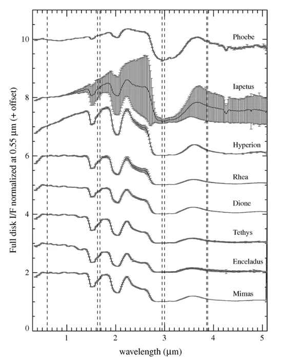
Figure 1. VIMS spectra of Saturn's icy moons, with the characteristic water ice bands at 1.5, 2., and 3 μm. The presence of non-icy compounds causes variations in albedo, VIS-NIR spectral slope, and UV downturn at 0.35-0.55 μm. Vertical dashed lines indicate VIMS' order sorting filter gaps. Adapted from [2].

By establishing appropriate spectral indicators (such as spectral slopes in the UV-VIS and VIS-NIR wavelength intervals and the depth of water ice absorptions) connected to regolith grain size and water ice/contaminant abundances, several studies examined the spectral and compositional variability of the MISS, providing qualitative trends of average properties [2, 3, 4] and at disk-resolved scales [5-7]. However, this approach was unable to fully characterize the compositional and physical properties from a quantitative standpoint, because this information is still at least partially entangled in the spectral indicators.

In an attempt to conduct a more quantitative analysis of the composition and physical characteristics of MISS's surfaces, VIMS hyperspectral data has been exploited through comparison with the outcomes of radiative transfer solutions (e.g., Hapke theory, 8), allowing to compute the spectra of different mixtures as a function of endmember abundances, mixing modalities, and grain size distributions. Such spectral modeling effort enables one to determine the spectral contribution of various compositional and physical properties to the observed spectral shape. In the case of MISS, similar attempts have been conducted in a small number of cases to constrain the composition of chosen terrains on selected targets (see [9] for Dione), or to determine the MISS compositional properties at full-disk scale [10, 2]. On the other hand, a systematic application of this methodology to perform a global compositional mapping from disk-resolved observations of MISS has not been performed yet.

In this paper, we set ourselves to this task, starting with the largest of Saturn's mid-sized icy moons, Rhea. To this end, we take advantage of VIMS photometrically-corrected disk-resolved data of the satellite, made available by [7]. This data, by minimizing the observation geometry bias, allows us to characterize the intrinsic specral and albedo variability of the surface and, by means of systematic spectral modeling, map the distribution of water ice and contaminants across the surface, along with the regolith grain size.

Method: we employ a VIMS photometrically-corrected spectral map of Rhea, adapting the methodology outlined in [7] (Figure 2, top panel). The spectral map is created by averaging photometrically corrected VIMS observations over a standard longitude-latitude grid with 0.5°x0.5° bin sampling. A hyperspectral cube with a spectrum assigned to each map position is the end product.

Using Hapke's theory, we conduct systematic spectral modeling for every bin in the spectral map. The surface is characterized as a mixture of water ice, a macromolecular organic compound (tholin, causing the UV absorption), and amorphous carbon (as a darkening contaminant), adopting a paradigm similar to previous modeling attempts [11].

Preliminary findings: we present a preliminary compositional map of Rhea in Figure 2 (middle panel). The spectral modeling results point to a surface composition dichotomy, where non-icy materials (carbon and tholin) are more abundant in the trailing hemisphere (longitudes 180°–360°) than in the leading one (longitudes 0°–180°), hosting larger amounts of water ice. The distribution of the various endmembers maps the albedo and color dichotomy of the surface, with a redder/darker trailing side contrasted to a bluer/brighter leading hemisphere (bottom panel of figure 2).

The inferred endmember spatial variability will be examined in light of the exogenous processes affecting Rhea's surface, such as photolysis, flux of charged particles driven by Saturn's magnetosphere, contamination of exogenic darkening material, and bombardment from E-ring grains [12], accounting for their longitudinal dependence, along with cratering and endogenous processes that shaped the surface of Rhea.

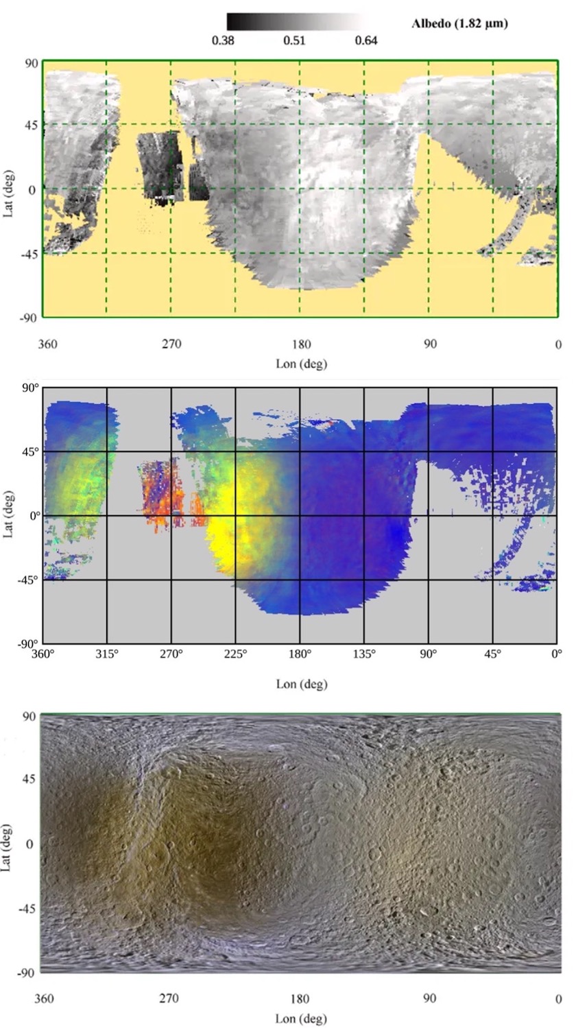
Figure 2. Top panel: 1.82-µm equigonal albedo map of Rhea in cylindrical projection [7]. Middle panel: RGB compositional map of Rhea (red: tholin abundance; green: carbon abundance; blue: water ice abundance). Bottom panel: Cassini Imaging Science Subsystem global color (IR, Green, UV) map (PIA18438, image credit P. Schenck, NASA/JPL-Caltech/Space Science Institute/Lunar and Planetary Institute).

Acknowledgments: This work is supported by the INAF data analysis grant "MId-sized Saturnian icy Satellites Investigation by Spectral modeling" (MISSIS).

References: [1] Brown et al., 2004. SSRv 115, 111–168. [2] Filacchione et al., 2012. Icarus 220, 1064–1096. [3] Filacchione et al., 2013. ApJ 766. [4] Hendrix, et al., 2018. Icarus 300, 103–114. [5] Stephan et al., 2016. Icarus 274, 1–22. [6] Scipioni et al., 2017. Icarus 290, 183–200. [7] Filacchione et al., 2022. Icarus 375. [8] Hapke, B., 2012. Theory of reflectance and emittance spectroscopy (Cambridge Univ. Press). [9] Clark et al., 2008. Icarus 193, 372–386. [10] Ciarniello et al., 2011. Icarus 214, 541–555. [11] Ciarniello et al., 2019. Icarus 317, 242-265. [12] Hendrix et al., 2018. Icarus 300, 103–114.

How to cite: Ciarniello, M., Filacchione, G., Raponi, A., Galluzzi, V., D'Aversa, E., and Gorga, B.: Mapping the surface composition of Rhea by means of spectral modeling, Europlanet Science Congress 2024, Berlin, Germany, 8–13 Sep 2024, EPSC2024-321, https://doi.org/10.5194/epsc2024-321, 2024.

EPSC2024-618
|
On-site presentation
Alice Le Gall, Salman Raza, Emmanuel Lellouch, Bryan Butler, Léa Bonnefoy, Cédric Leyrat, Frédéric Schmidt, Cyril Mergny, Colas Robin, François-Xavier Meyer, and Lucy Harrar

Introduction

Saturn’s icy satellites, in synchronous rotation around Saturn, often display large differences between their leading (L) and trailing (T) sides, which interact differently with their orbital environment and, in particular, with Saturn’s dust rings. Indubitably, the most dramatic hemispheric dichotomy in the Saturnian system occurs at Iapetus, whose T side and poles are about an order of magnitude optically brighter than most of its L hemisphere. The origin of this two-tone coloration has long been controversial; thanks to the observations of the Cassini mission which explored the Saturnian system from 2004 to 2017, there now seems to be a consensus toward an exogenic deposition of low-albedo materials originating from Phoebe’s vast debris ring that crosses Iapetus’ orbit [e.g., 1, 2, 3]. However, questions remain about the composition and vertical extent of Iapetus’ L hemisphere dark deposit. Measuring the thermal emission from Iapetus at different wavelengths, thus probing different depths, can help answering these questions. In particular, probing the L side of Iapetus at multiple centimetric wavelengths can put a firmer number on the thickness of the dark layer thus bringing key constraints for dynamical models aiming at reproducing dust distribution on Iapetus [e.g., 4]. That is why, in 2017, we have launched an observing campaign to collect spatially-resolved observations of Iapetus from the Jansky VLA (Very Large Array)  telescope. So far, a total of 30 hours of observations were collected [5].

Radio maps of Iapetus

The VLA telescope is an interferometry radio-telescope consisting of 28 antennas organized in a Y shape in the plains of San Agustin in New Mexico, USA. Since 2018, it was used to measure the thermal emission from Iapetus at various wavelengths from 0.7 to 6.0 cm i.e., in the Q, Ka, K, Ku, X and C bands. A total of 11 radio maps were built from these observations; Fig 1 displays 7 of them. They all probe Iapetus dayside, considering the location of the Saturn system and the Earth in relation to the Sun but with different portions of the leading side in the visible disk. The most resolved maps (28 May and 3 June 2018) show an asymmetry in the emitted flux with more flux coming from the dark face of Iapetus than from the bright face, implying that the latter is colder or at least less emissive. In addition to VLA observations, Iapetus’s thermal emission was also mapped in 2007 by the radiometer on board the Cassini probe at 2.2 cm [6].

Fig. 1:  Maps of Iapetus’ thermal flux collected in 2018, 2019 and 2021 from the JVLA (Very Large Array telescope, New Mexico, USA) at different wavelengths/bands in the microwave domain. Insets indicate the size of the primary beam and the albedo map of the visible disk.

Thermal emission model

The interpretation of VLA maps requires a thermal emission model. The model we developed combines a thermal model, providing the physical temperatures profiles (K) in Iapetus’ subsurface at different latitudes and longitudes, a transfer radiative model, to produce brightness temperature (K) maps of Iapetus which can be converted into radiance (erg.cm−2.s−1/sr−1) and then integrated over the beam (flux in Jy/beam) associated to each observation.

Thermal model - We adapted a multilayer model called “Multi-layered Implicit Heat Transfer Solver” (MultIHeaTS) [7] to the case of Iapetus. The unique source of heat is the Solar flux. The leading side subsurface consists in a top layer (the dark dust layer) overlying a bottom layer (the water ice crust) while a water ice monolayer is assumed for the trailing side. The main parameters of the bi-layer model are the porosities of each layer (which primarily controls the effective thermal inertia) and the thickness of the top layer (which, based on ground-based observations from the Arecibo 12.6-cm radar system should not exceed a few meters [8]). At cm wavelengths, the emission depth is expected to be larger than the depth of penetration of the diurnally-varying solar insolation. As a consequence, the sensed subsurface temperatures are a combination of diurnal and seasonal components and the thermal model is set to provide temperature profiles down to tens of meter depths.

RT model - We tested two multi-layer radiative transfer models: (i) a model proposed by [9] for RT in stratified agricultural soils which assumes smooth and flat buried interfaces with no scattering within the layers, (ii) the Snow Microwave Radiative Transfer (SMRT) model designed for snow or sea-ice [10], which considers wave scattering, absorption, reflection, and transmission. Both models take as inputs temperature profiles and their main parameter is the complex dielectric permittivity of the dark dust.

Preliminary results

In this presentation, we will compare observations to model predictions for various combinations of parameters looking for the parameter combination that best reproduces the observations. As an example, Fig. 2a shows the best-fit model for the observation of May 28, 2018; it was obtained for a dark layer of thickness 1 cm and made of organic materials with the [9] model. The L/T asymmetry is well reproduced but the residual map suggests that the emissivity of the T side is overestimated by the model while it is the opposite on the L side (Fig. 2b). This likely like indicates that volume scattering in the water ice crust cannot be neglected. Predictions using the [10] model should therefore lead to better fits.


Fig. 2: (a) Best-fit model for the observation of May 28, 2018. (b) Residual map (data-model).

 References

1. Buratti et al., 2002, Icarus 155, 375–381

2. Verbiscer et al., 2009, Nature 461, 1098.

3. Dalle Ore et al., 2012, Icarus 221 (2), 735–743

4. Tamayo et al. 2011, Icarus 215, 260

5. Bonnefoy et al., 2024, Icarus 41, 115950

6. Le Gall et al., 2014, Icarus 241, 221–238

7. Mergny and Schmidt, submitted

8. Ostro et al., 2006, Icarus 183 (2), 479–490.

9. Burke et al., 1979, J. Geophys. Res., 84( C1), 287– 294

10. Picard and al., 2018, Geoscientific Model Development 11, 2763–2788

How to cite: Le Gall, A., Raza, S., Lellouch, E., Butler, B., Bonnefoy, L., Leyrat, C., Schmidt, F., Mergny, C., Robin, C., Meyer, F.-X., and Harrar, L.: Iapetus: Investigating the most dramatic hemispheric dichotomy in the Solar system with radio observations, Europlanet Science Congress 2024, Berlin, Germany, 8–13 Sep 2024, EPSC2024-618, https://doi.org/10.5194/epsc2024-618, 2024.

EPSC2024-71
|
ECP
|
On-site presentation
Xiao Jin Xi and Alain Vienne

Numerical integration ephemerides are highly valued in both research and engineering due to their exceptional precision. However, their application in theoretical studies, particularly in the investigation of rotation and evolution, is constrained by their finite available time spans. In our previous work, we effectively explored the analytical representation of the mean longitude of Titan from the Jet Propulsion Laboratory (JPL) ephemeris. We established this representation as a function of combinations of proper frequencies and related the results with what is given in the synthetic ephemerides obtained by the Théorie Analytique des Satellites de Saturne (TASS).

In this study, we extend our analytical representations beyond the mean longitude to the other osculating elements of the Titan ephemeris. This allows us to create new synthetic representations that combine the benefits of both systems: the enduring stability and system intricacies of TASS, along with the exceptional precision characteristic of numerical integration ephemerides. These combinations encompass vital dynamical information, including the proper frequencies, which will be valuable for theoretical research.


How to cite: Xi, X. J. and Vienne, A.: Analytical Representation of Saturnian Satellite Numerical Ephemerides over Limited Time Spans, Europlanet Science Congress 2024, Berlin, Germany, 8–13 Sep 2024, EPSC2024-71, https://doi.org/10.5194/epsc2024-71, 2024.

EPSC2024-189
|
On-site presentation
Valery Lainey, Nicolas Rambaux, Gabriel Tobie, Nick Cooper, Qingfeng Zhang, Benoit Noyelles, and Kevin Baillié

During the thirteen years spent in orbit around Saturn before its final plunge, the Cassini probe provided more than ten thousand astrometric observations of moons. Such a large amount of precise data has allowed us to search for extremely small signals in the orbital motion of the Saturnian satellites. These signals can be linked to key physical mechanisms at play in the system, opening the doors to a new vision of the Saturn system. Using more than a century of ground-based astrometric observations, and benefiting from Cassini imaging data, we have studied the orbital motion of all of Saturn's inner and main moons, including those recently discovered by the Cassini probe. We show how astrometry has allowed us to characterize the strong tidal effects acting among the Saturnian system, while assessing the interior characteristics of several moons and their primary, including the discovery of Mimas' ocean. Updated results are presented.

How to cite: Lainey, V., Rambaux, N., Tobie, G., Cooper, N., Zhang, Q., Noyelles, B., and Baillié, K.: Latest astrometric results for the Saturnian system, Europlanet Science Congress 2024, Berlin, Germany, 8–13 Sep 2024, EPSC2024-189, https://doi.org/10.5194/epsc2024-189, 2024.