Poster presentations and abstracts
Mercury Science in the post-MESSENGER area, open to all Mercury relating subjects, and covering e.g.
- Mercury's interior, surface, environment, and interactions thereof
- BepiColombo Mercury Science
- BepiColombo Flyby (Earth, Venus, Mercury) and Cruise (Radio Science, Solar Wind, Gamma Rays): results and expectations
- Ground-based Mercury Observations: results and plans
- laboratory activities in support of Mercury Science
Session assets
The Mercurian Gamma-ray and Neutron Spectrometer (MGNS) is a scientific instrument developed to study the elementary composition of the Mercury’s sub-surface by measurements of neutron and gamma-ray emission of the planet. MGNS measures neutron fluxes in a wide energy range from thermal energy up to 10 MeV and gamma-rays in the energy range of 300 keV up to 10 MeV with the energy resolution of 5% FWHM at 662 keV and of 2% at 8 MeV. The innovative crystal of CeBr3 is used for getting such a good energy resolution for a scintillation detector of gamma-rays.
During the BC long cruise to Mercury, it is planned that the MGNS instrument will operate practically continuously to perform measurements of neutrons and gamma-ray fluxes for achieving two main goals of investigations.
The first goal is monitoring of the local radiation background of the prompt spacecraft emission due to bombardment by energetic particles of Galactic Cosmic Rays. This data will be taken into account at the mapping phase of the mission on the orbit around Mercury. Detailed knowledge of the spacecraft background radiation during the cruise will help to derive the data for neutron and gamma-ray emission of the planet at the mapping stage of the mission because many elements, like Mg, Na, O and others, the abundance of which at the uppermost layer of the planet is studied, are also present in the material of the spacecraft. Indeed, the nuclear lines of Al, Mg and O are well-pronounced in the spectrum, which are also expected to be detectable in the gamma-ray spectrum of the Mercury emission.
The second goal of MGNS cruise operations is the participation in the Inter Planetary Network (IPN) program for the localization of sources of Gamma-Ray Bursts in the sky. In fact, the localization accuracy by the interplanetary triangulation technique is inversely proportional to the distance between the spacecrafts that jointly detected a GRB. Before the launch of BepiColombo, the IPN network included a group of spacecrafts in the near-to-Earth orbit (e.g. Konus-Wind, Fermi-GBM, INTEGRAL, Insight-HXMT) and the Mars Odyssey spacecraft on the orbit around Mars. Now, MGNS provides another interplanetary location, potentially increasing the accuracy of GRBs localization. During the first 13 months of continuous operation, MGNS detected 24 GRB's. Pre-set value of time resolution for continuous measurements of profiles of GRBs is 20 seconds. Since of November 14, 2019, the BC Mission Operation Centre has allocated downlink resources to run MGNS continuously in a 1 sec time resolution for GRB measurements. The GRB detection rate, based on data with a time resolution of 1 sec is about 2-3 GRB's per month.
Gamma-rays of solar flares are also detectable by MGNS. Solar flares are nonstationary and anisotropic processes and the ability to observe them from different directions in the Solar system is crucial for further understanding their developments and propagation, as it was demonstrated in the case of HEND instrument on board Mars Odyssey. The Sun cycle is presently around its minimum, and MGNS has not detected any solar events during its first 7 months of the cruise, but the flight to Mercury is long enough and many future flares are expected to be detected.
The MGNS instrument will also perform special sessions of measurements during flybys of Earth, Venus and Mercury with the objective to measure neutron and gamma-ray albedo of the upper atmosphere of Earth and Venus and of the surface of Mercury. Another objective is to test the computational model of the local background of the spacecraft using the data measured at different orbital phases of flyby trajectories. The low altitude flybys (such as the 700 km flyby for Venus and three 200 km flybys for Mercury) would be the most useful for such tests being BC maximally shadowed for cosmic radiation by the actual planet. Neutron and gamma-ray measurements during Earth flybys enable investigation of interaction between solar wind and Earth environments as well as studies of spacecraft neutron and gamma-ray background upon its passage through the Earth's radiation belts.
How to cite: Kozyrev, A., Litvak, M., Sanin, A., Malakhov, A., Mitrofanov, I., Owens, A., Schulz, R., and Quarati, F.: MGNS experiment science investigations during BepiColombo cruise, Europlanet Science Congress 2020, online, 21 Sep–9 Oct 2020, EPSC2020-389, https://doi.org/10.5194/epsc2020-389, 2020.
Planetary Space Weather is the discipline that studies the state of the Sun and how it interacts with the interplanetary and planetary environments. It is driven by the Sun’s activity, particularly through large eruptions of plasma (known as coronal mass ejections, CMEs), solar wind stream interaction regions (SIR) formed by the interaction of high-speed solar wind streams with the preceding slower solar wind, and bursts of solar energetic particles (SEPs) that form radiation storms. This is an emerging topic, whose real-time forecast is very challenging because among other factors, it needs a continuous coverage of its variability within the whole heliosphere as well as of the Sun’s activity to improve forecasting.
The long cruise of BepiColombo constitutes an exceptional opportunity for studying the Space Weather evolution within half-astronomical unit (AU), as well as in certain parts of its journey, can be used as an upstream solar wind monitor for Venus, Mars and even the outer planets. This work will present preliminary results of the Space Weather conditions encountered by BepiColombo since its launch until mid-2020, which includes data from the solar minimum of activity and few slow solar wind structures. Data come from three of its instruments that are operational for most of the cruise phase, i.e., the BepiColombo Radiation Monitor (BERM), the Mercury Planetary Orbiter Magnetometer (MPO-MAG), and the Solar Intensity X-ray and particle Spectrometer (SIXS). Modelling support for the data observations will be also presented with the so-called solar wind ENLIL simulations.
How to cite: Sanchez-Cano, B., Moissl, R., Heyner, D., Huovelin, J., Mays, M. L., Odstrcil, D., Lester, M., Bunce, E. J., James, M. K., Witasse, O., and Benkhoff, J.: Preliminary results of Space Weather conditions encountered by BepiColombo during the first phase of its cruise, Europlanet Science Congress 2020, online, 21 Sep–9 Oct 2020, EPSC2020-689, https://doi.org/10.5194/epsc2020-689, 2020.
BepiColombo (ESA/JAXA), Solar Orbiter (ESA/NASA) and Parker Solar Probe (NASA), will be all traveling in the inner heliosphere for 5 years, between the launch of Solar Orbiter (10th February 2020) and the end of the cruise phase of BepiColombo (2018 - 2025). During the five years to come, these three spacecraft missions will cover different radial distances: BepiColombo will evolve between the orbit of Mercury up to Earth (0.3 AU and 0.9 AU), while Solar Orbiter’s highly elliptical orbit will cover distances from 1.02 AU to 0.28 AU, and Parker Solar Probe from about 0.7 AU to 0.04 AU. In addition to these missions, previous and future spacecraft missions will be taking measurements in our solar system (from Venus ~ 0.7 AU till Jupiter 5 AU). The exceptional and complementary plasma instrumental payloads and magnetometers on-board the different satellites will allow us to make unique multi-point measurements in the solar wind. Hence, in this work, we present the potential coordinated observations between at least BepiColombo, Solar Orbiter and Parker Solar Probe (including also other satellites such as probes at L1, or around Venus, Mars and Jupiter). More specifically, in the first part we focus on the different scientific topic that could be studied during the cruise phase of BepiColombo, in the second part we present the related potential operational instruments and in the last part we discuss the different windows of opportunities we have investigated based on different spacecraft geometries.
How to cite: Hadid, L. and the BepiColombo coordinated observations working group: Coordinated measurements during the Cruise phase of BepiColombo: science cases, operational instruments and windows of opportunities, Europlanet Science Congress 2020, online, 21 Sep–9 Oct 2020, EPSC2020-633, https://doi.org/10.5194/epsc2020-633, 2020.
Abstract:
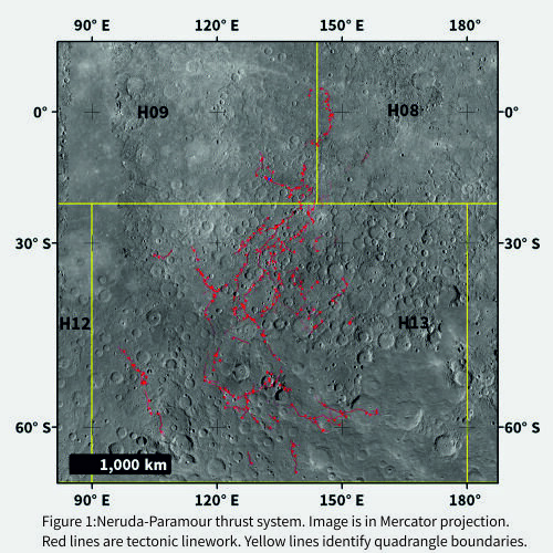
Our tectonic mapping as part of a larger morphostratigraphic mapping effort of the H13, Neruda Quadrangle (1) has led us to recognise the “Neruda-Paramour” thrust system. The system appears to extend from the southern limits of H13 north through H09 and H08 and simplifies at its northern end into Paramour Rupes (Figure 1). Mercury’s tectonic evolution is dominated by global scale contractional structures of which the Neruda-Paramour system is part of (2). These structures are believed to have formed either by secular cooling of the planet (3), tidal despinning (4), mantle overturn (5), true polar wander (6) or a combination of these processes. Regardless of the process, Mercury’s surface exhibits abundant evidence of global contraction in the form of shortening structures such as lobate scarps, high relief ridges and wrinkles ridges (7,8). These features are widely accepted as the surface expressions of thrust faulting and folding, produced by lithospheric horizontal compression. Often, these contractional features comprise major thrust systems as linked segments with a consistent trend (8). In order to understand the development of the Neruda-Paramour system and to ascertain if there is any sequence of movements, we are first mapping the system in its entirety followed by age dating of each thrust segment’s last movement using the buffered crater counting (BCC) technique.
Methods:
Tectonic lineament mapping
Primary basemap: Global ~166 mpp v1.0 BDR tiles with moderate (~74°) solar incidence angles.
Secondary basemaps: low (~45°) and high (~78°) incidence angle basemaps, ~665mpp enhanced colour mosaic; MLA- and stereo-derived DEMs.
Scale: 1:3M scale with digitisation at 1:300k.
Software: Esri ArcGIS 10.5.1 GIS software.
Buffered crater counting
Software: Esri ArcGIS 10.5.1 GIS software with CraterTools extension (9). CraterStats 2.0 (10).
We use the BCC technique by (8,11) which counts craters that are unfaulted and undeformed by the structures under investigation to derive absolute model ages of linear landforms. The BCC technique uses a buffer zone around the linear feature to include more craters to be taken into consideration for the crater size frequency distribution (CSFD) count. This addition of included craters produces a more robust measurement, which is important due to the restricted surface area that the structures occupy (12). We have chosen to consider all craters that directly intersect the structures ≥2 km. A fault buffer width of 2R (R=radius of the crater) for buffer generation is used. CSFD data is exported to CraterStats 2.0 where it is plotted in a log Ncum (cumulative crater frequency) vs log D (diameter) and using the production function (PF) a best fit of the CSFD data is made, giving an absolute model age value. The Neukum Production Function and Le Feuvre and Wieczorek Production Function are used and the results from each are compared. Method after (8).
Results:
We will present our analysis of the mutual age relationships between elements of the Neruda-Paramour thrust system and discuss the implications for the tectonics of this part of the globe.
Acknowledgements:
Mapping is in association with Planmap, funded through the EU Horizon 2020 research and innovation programme under grant agreement No. 776276. Ben Man is supported by STFC and the Open University’s Space Strategic Research Area.
References:
How to cite: Man, B., Rothery, D. A., Balme, M. R., Conway, S. J., and Wright, J.: Investigating the Neruda-Paramour thrust system, Mercury, Europlanet Science Congress 2020, online, 21 Sep–9 Oct 2020, EPSC2020-794, https://doi.org/10.5194/epsc2020-794, 2020.
Introduction
Boulders, meters-size blocks of rock, are seen in great numbers in high-resolution images of the Moon, Mars, and small bodies. Boulders and their geological associations provide information about surface processes on these bodies. Here we report on rarity of boulders on Mercury, and discuss possible implications of this.
Rarity of boulders on Mercury
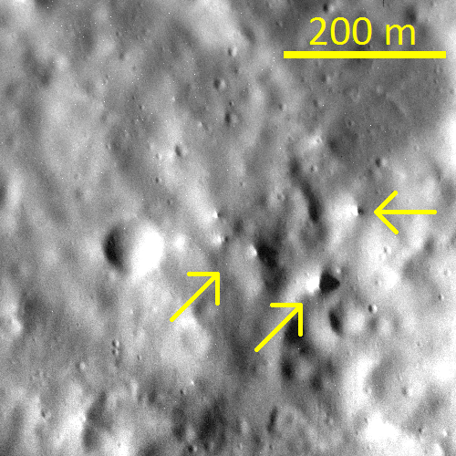
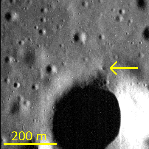
We studied boulders on Mercury with high-resolution images acquired by MDIS NAC camera onboard MESSENGER. We screened all ~3000 images of the highest resolution (<2.5 m/pix sampling) and acceptable quality, and found discernable boulders only in 14 of them (see examples in Fig. 1,2) [1]. The highest resolution images are small (0.25 Mpix), have a considerable smear, low signal-to-noise ratio, and are separated by large distances; they can be considered as random samples of surface morphology in a region limited by 40 – 70°N and 210 – 320°E, which is occupied mostly by the intercrater plains. The majority of the found boulders are associated with a single large young impact crater (Fig. 1), and a few boulders are associated with small impact craters (Fig. 2). With the available images, it is impossible to distinguish between intact boulders and debris piles of disintegrated or partly disintegrated boulders, therefore such (partly) disintegrated boulders are included in our boulder count.
To compare Mercury with the Moon, we extracted similar random 0.25 Mpix samples from LROC NAC images that have the same sampling, the same solar illumination incidence angle and are situated in highlands. We artificially degraded image quality to mimic MDIS NAC quality. Then we screened these image samples searching for boulders and found them at ~15% of the random sample images. Thus, boulders on Mercury are extremely rare in comparison to the Moon (~ 30x less abundant).
Possible causes
Boulder population on the Moon is dynamic: the characteristic boulder lifetime is ~100 Ma [2], and the observed population represents equilibrium between boulder formation and obliteration. The same obviously occurs on Mercury. Therefore, much sparce boulder population can occur due to a lower production rate, a shorter lifetime, or both.
Production rate. Boulders on the Moon occur in association with (1) fresh impact craters of different sizes and (2) hilltops, upper edges of rilles, and other convex relief forms. Respectively, there are two mechanisms of boulder formation: (1) bedrock fragmentation and excavation by impacts, and (2) progressive exposure of pre-existing blocks and fractured bedrock by removal of regolith layer from convex relief by diffusive creep. On Mercury we observe boulders in the first type of settings (craters) only. The intercrater plains on Mercury are significantly smoother than the lunar highlands [3], therefore suitable hilltops may be less abundant and might not be sampled in our limited image set. Thus, the general smoothness of Mercury in comparison to the Moon [3] may contribute to a lower boulder production rate.
Regolith on Mercury is thought to be thicker than on the Moon [3,4]. The smallest craters are forming in regolith and cannot excavate boulders. Due to the thicker regolith, the onset crater size for boulder formation is larger. Since the crater formation rate on Mercury is on the same order of magnitude, the larger onset crater size means a lower rate of boulder-forming impacts, and therefore, a lower boulder formation rate. However, these two factors seem insufficient to explain the huge difference in boulder occurrence between the Moon and Mercury.
Lifetime. Boulders are destroyed by small meteoritic impacts, ground by micrometeoritic impacts [2], and cracked and disintegrated by thermal stresses [5,6]. The relative role of these processes on the Moon is controversial. Since meteoritic flux is on the same order of magnitude on both bodies, it cannot account for the observed huge difference.
Peak daytime temperature at a flat monolith bedrock surface induces tensile stress equal to E α ΔT/(1-ν), where E is the Young’s modulus (~60 GPa for basalts [7]), ν is Poisson ratio (~0.25), α is linear thermal expansion coefficient (~10-5 K-1), and ΔT is the peak temperature excess above the mean temperature. For Mercury, this stress would regularly exceed 100 MPa. This value gives an order of magnitude estimate for peak tensile stress experienced by a boulder, if it is larger or comparable to the diurnal thermal skin depth for solid rock, which is ~3 m for the long day on Mercury. For smaller boulders the peak stress is lower; detailed modeling has been done in [5]. The boulders we observe are larger than 3 m, therefore, the peak stress is on the order of 100 MPa, much higher than a typical tensile strength of intact basalts (~14 MPa [7]). Therefore, all boulders acquire boulder-scale fractures at their first exposure at the surface. The difference Δα between thermal expansion coefficients of rock-forming mineral grains leads to thermal stress at grain scale [6]. They are scaled as C E Δα ΔT, where C depending on ν and grain geometry is on the order of unity. These stresses would also routinely exceed tensile strength; they would lead to formation of microfractures at grain scale. Thus, thermal stresses cause extensive fracturing of rocks on Mercury, which likely contributes to the short boulder life time.
The micrometeoritic flux on Mercury is significantly higher than on the Moon [8,9]. If micrometeoritic grinding is the dominant boulder obliteration mechanism on the Moon, then the difference in the micrometeoritic flux is likely to be sufficient to account for the entire observed difference in boulder abundance.
References
[1] Zharkova A. et al. (2019) LPSC 50, 1162.
[2] Basilevsky A.T. et al. (2013) PSS 89, 118-126.
[3] Kreslavsky M. et al. (2014) GRL 41, 8245-8251.
[4] Zharkova A. et al. (2015) AGU Fall, P53A-2099.
[5] Molaro J. et al. (2017) Icarus 294, 247-261.
[6] Molaro J. et al. (2015) JGR 120, 255-277.
[7] Schultz R. (1993) JGR 98, 10883-10895.
[8] Cintala M. (1992) JGR 97, 947.
[9] Borin P. et al. (2009) Astron. Astrophys. 503, 259.
How to cite: Kreslavsky, M. A., Zharkova, A., and Gritsevich, M.: Rarity of Boulders on Mercury: Possible Causes, Europlanet Science Congress 2020, online, 21 Sep–9 Oct 2020, EPSC2020-958, https://doi.org/10.5194/epsc2020-958, 2020.
The optical constant of the material, meaning the complex refractive index m=n+i k, is an essential parameter when considering the reflection and absorption properties of that material. The refractive index is a function of wavelength of the light, and usually the imaginary part k is what governs the reflection or transmission spectral behavior of the material.
The knowledge of the complex refractive index as a function of wavelength, m(λ), is needed for light scattering simulations. On the other hand, rigorous scattering simulations can be used to invert the refractive index from measured or observed reflection spectra. We will show how the combination of geometric optics and radiative transfer codes can be used in this task.
In this work, the possible application is with the future visual-near infrared observations of Mercury by the ESA BepiColombo mission. That application in mind, we have used four particulate igneous glassy materials with varying overall albedo and in several size fractions in reflectance spectra measurements (hawaiitic basalt, two gabbronorites, anorthosite, see details from Carli et al, Icarus 266, 2016). The grounded material consist of particle with clear edges and quite flat facets, and we choose to model the particle shapes by geometries resulting from Voronoi division of random seed points in 3D space (see Fig. 1).
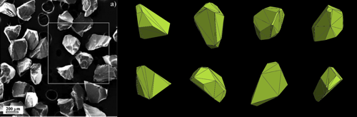
Figure 1. On the left, a SEM image of anorthosite particles, size fraction 224–250 µm (from Carli et al, Icarus 266, 2016). On the right, eight example particles from Voronoi division algorithm.
The refractive index inversion is done here using first a geometric optics code SIRIS (Muinonen et al, JQSRT 110, 2009) to simulate the average Mueller matrix, albedo, and scattering efficiency for a single Voronoi particle. Then, these properties are fed into radiative transfer code RT-CB (Muinonen, Waves in Random Media 14, 2004) to produce the reflective properties of a semi-infinite slab of these particles. This procedure is repeated for a 2D grid of particle size parameters x=2πr/λ, where r is the radius of particle, and imaginary part k of refractive index. In Vis-NIR wavelengths, the real part n is quite constant and is estimated to be about 1.58 for all the four glasses. From the simulated slab reflectance data with the 2D x, k parameter grid, we can first interpolate, and then invert the k parameter for any reflectance value with given wavelength and particle size.
The resulting spectral behavior of k for the four glasses and for all the size fractions was seems very realistic. Carli et al. (Icarus 266, 2016) inverted the k spectral behavior for these same samples using Hapke modeling, and the results are quite similar. An example of inverted k for one sample (anorthosite) is shown in Fig. 2.

Figure 2. Inverted imaginary part of refractive index, k, as a function of wavelength for different size fractions of anorthosite.
We show that rigorous light scattering simulations can be used to invert the optical constant of a material from observed reflectance spectra, at least if some assumptions regarding particle sizes can be done. These methods can be valuable when analyzing various illumination and observing geometries, intimate mixtures of multiple materials, and other cases where Hapke modeling might not be enough for accurate inversion. We foresee employing these methods to analyze the observations of Mercury from ESA BepiColombo mission.
Acknowledgements: Research supported, in part, by the Academy of Finland (project 325805).
How to cite: Penttilä, A., Väisänen, T., Martikainen, J., Carli, C., Capaccioni, F., and Muinonen, K.: Rigorous inversion of absorption coefficient from spectral properties of particulate material, Europlanet Science Congress 2020, online, 21 Sep–9 Oct 2020, EPSC2020-381, https://doi.org/10.5194/epsc2020-381, 2020.
Mercury geology reached a new era after the MESSENGER mission, which has allowed not only to acquire global information but also to study the geological history of the planet with multiple techniques. The orbital BepiColombo mission will be the next step to fix some of the Hermean paradigm because more techniques, coupled with the higher resolution of the instruments onboard Mio and Bepi.
Integration of compositional data and morpho-stratigraphic maps generally produced from camera data, will be one of the main issue to improve the understanding of Mercury geological evolution. This goal is also correlated with the efforts of other projects such as PLANMAP European H2020 and GMAP Europlanet 20-24.
Several morpho-stratigraphic maps of Mercury quadrangles have been produced, or are ongoing (e.g. Galluzzi et al. 2018), and a global map has been realized (e.g. Kinczyk et al. 2019). Discussion or integration at quadrangle level of Mercury is recently beginning (e.g. Bott et al. 2019; Zambon et al. 2019) and here we report activity done in the Kuiper H06.
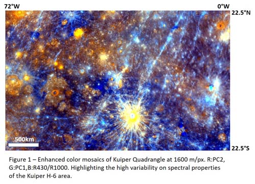
Kuiper (H06) is an equatorial quadrangle, and it encompasses the area between longitudes 72°W –0° and latitudes 22.5°N – 22.5°S. H06 morpho-stratigraphic mapping is still ongoing (Giacomini et al. 2018; 2019), it evidences a high variegation of units, from older intercrater plains to younger smooth plains, to craters. Several craters show pyroclastic deposits (e.g. Kerber et al. 2011; Pajola et al. 2020), in some cases with putative vents, and hollows. Some of the hollows look like very peculiar from spectral point of view, e.g. in Dominici Crater (Vilas et al. 2016; Lucchetti et al. 2018), showing possible indication of mineralogical phases. Whereas most smooth plains are limited in extension and confined on the floor of the largest craters, a wide smooth plain has been detected that surrounds Rudaki crater. Some of these plains show clearly color variegation (e.g. two color units within Renoir Basin, see Giacomini et al. 2018).
Due to the low latitudes, the coverage from MDIS data with high spatial resolution is lower than the northern quadrangles (e.g. Bott et al. 2019; Zambon et al. 2019) and we approach the study in a multiple-stage passages. This has been done to investigate the region with the best detail from a spectral point of view. Following the mosaic product procedure used by Zambon et al. (2019), we generate a homogeneous 8 color global mosaic at 1600 m/px scale (average scale taking into account the average resolution) and at 665 m/px pushing the resolution. Moreover, we considered the partial quadrangle coverage mosaics at 385 m/px and 246 m/px to exploit the presence of higher resolution color images.
We will show spectral variations considering specific indices and color combinations (example on Figure 1), discussing the possibility to define some spectral units which could be later integrated with the morpho-stratigraphic mapping. Furthermore, we will locally investigate the spectral variation of specific cases, e.g. fresh craters, hollows and pyroclastic material, to infer some indication on material composition, or within some blue dark regions to understand the possible darkening material.
This activity could be also helpful in the definition of indicators improving the selection procedure for regions of interest (see also Giacomini et al. 2020) to be studied for covering the science goals of the BepiColombo mission (e.g. Rothery et al. 2020).
Acknowledgements:
We gratefully acknowledge funding from the Italian Space Agency (ASI) under ASI-INAF agreement 2017-47-H.0. MM, CC, FZ, FA were also supported by European Union’s Horizon 2020 research grant agreement No 776276- PLANMAP. MM, CC, FA were also supported by Europlanet 20-24 GMAP, EPN-RI-2024.
References:
Bott N., et al. 2019. Global Spectral Properties and Lithology of Mercury: The Example of the Shakespeare (H‐03) Quadrangle. JGR-Planets, 124, 2326-2346.
Zambon F., et al. 2019. Spectral properties of the H05 Hokusai quadrangle on Mercury and relationship with the morpho-stratigraphic units. EGU 7796.
Giacomini L., et al. 2018. Updates on geologic mapping of Kuiper (H06) quadrangle. EPSC 721-1.
Giacomini L., et al. 2019. GEOLOGICAL MAPPING OF THE KUIPER (H06) QUADRANGLE OF MERCURY. XV Congresso delle Scienze Planetarie, pg. 71.
Giacomini L., et al. 2020. Scientific sites of interest in Kuiper Quadrangle (H06). EPSC this meeting.
Kerber L., et al. 2011. The global distribution of pyroclastic deposits on Mercury: The view from MESSENGER flybys 1–3. PSS, 59, 1895–1909.
Kinczyk M.J., et al. 2019. The First Global Geological Map of Mercury. EPSC-DPS 1045-1.
Lucchetti A., et al. 2018. Mercury Hollows as Remnants of Original Bedrock Materials and Devolatilization Processes: A Spectral Clustering and Geomorphological Analysis. JGR-Planets, 123, 2365-2379.
Pajola M., et al. 2020. MULTIDISCIPLINARY ANALYSIS OF LERMONTOV CRATER ON MERCURY. 51 LPSC 1402.
Rothery et al. 2020. Rationale for BepiColombo studies of Mercury’s surface and composition. Spa.Sci.Review. in press.
Vilas F., et al. 2016. Mineralogical indicators of Mercury's hollows composition in MESSENGER color observations. JGR 43, 1450-1456.
How to cite: Carli, C., Giacomini, L., Zambon, F., Ferrari, S., Massironi, M., Galluzzi, V., Altieri, F., Capaccioni, F., Ferranti, L., and Palumbo, P.: Kuiper Quadrangle spectral analysis: looking forward to integrated geological map, Europlanet Science Congress 2020, online, 21 Sep–9 Oct 2020, EPSC2020-367, https://doi.org/10.5194/epsc2020-367, 2020.
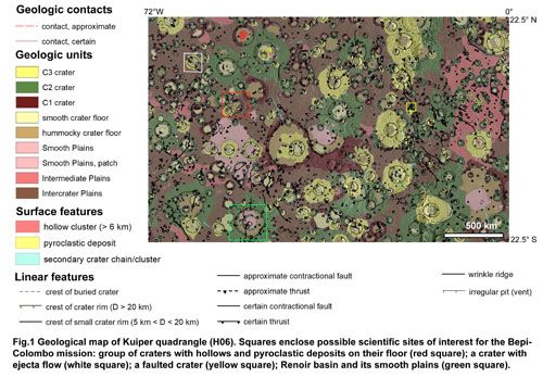
Kuiper quadrangle (H06) is located at the equatorial zone of Mercury and encompasses the area between longitudes 288°E – 360°E and latitudes 22.5°N – 22.5°S. A detailed geological map (1:3M scale) of the Kuiper quadrangle based on the high resolution MESSENGER data, was performed (Giacomini et al., 2018) (Fig.1).
The main basemap used for H06 mapping was the MDIS (Mercury Dual Imaging System) 166 m/pixel BDR (map-projected Basemap reduced Data Record) mosaic. Additional datasets were also taken into account, such as DLR stereo-DEM of the region (Preusker et al., 2017), mosaics with high-incidence illumination from the east and west, and MDIS global color mosaic (Denevi et al., 2018). The geological map showed that the quadrangle is characterized by a prevalence of crater materials which were distinguished into three classes based on their degradation degree (Galluzzi et al., 2016): from C1, consisting on the most degraded craters, to C3, including the freshest ones. Different plain units were also identified and classified on the basis of their density of craterisation: (i) intercrater plains, densely cratered, (ii) intermediate plains, moderately cratered and (iii) smooth plains, poorly cratered. Finally, several structures, mainly represented by thrusts, were mapped all over the quadrangle.
The mapping of quadrangle allowed the identification of canditate targets for the BepiColombo mission to Mercury (Fig.1). Indeed, volcanic features, as hollows and pyroclastic deposits, are widespread in the quadrangle. Their high-resolution analysis could give new information regarding the volcanism history on the planet.
Also several faulted craters have been detected. They represent important indicators to understand the kinematic of the structures transecting the craters (e.g. Galluzzi et al., 2015). Therefore, they will allow us to gain new clues on the tectonic history of the planet surface, with important implications for the knowledge of the thermophysical evolution of Mercury.
Further intriguing features are craters showing smooth ejecta with sinuous edges and a fluidized morphology. They have been called ejecta flows and they are thought to represent dry granular flows, although the presence of volatiles involved in the fluidization process can not be excluded (Xiao, 2013). Hence, high resolution data could give new inputs for the knowledge of the origin and evolution of these deposits.
Where MDIS WAC images at high spatial resolution are available, a more detailed analysis of the spectral behaviour of the surfaces can be accomplished (Carli et al., 2020). This allowed us to integrate geomorphological and spectral characteristics for specific areas in order to obtain new information about the landforms’ origin. Such procedure was preliminary conducted on Renoir basin, where two smooth deposits, showing different spectral characteristics, have been detected in different areas of its floor. However, a higher spectral and spatial resolution are needed to better appreciate the differences on those deposits.
In light of these evidences, it appears that the high resolution of the instruments of BepiColombo mission, like STC and HRIC cameras and VIHI spectrometer of SIMBIO-SYS, can significantly contribute to answer several questions raised during the geological mapping and analysis of the Kuiper quadrangle.
Acknowledgements
We gratefully acknowledge funding from the Italian Space Agency (ASI) under ASI-INAF agreement 2017-47-H.0. MM, CC, FZ were also supported by European Union’s Horizon 2020 research grant agreement No 776276- PLANMAP.
References
Carli et al., 2020. Kuiper Quadrangle spectral analysis: looking forward to integrated geological map. EPSC, this conference.
Denevi et al., 2018. Calibration, Projection, and Final Image Products of MESSENGER’s Mercury Dual Imaging System. Space. Sci. Rev., 214: 2. https://doi.org/10.1007/s11214-017-0440-y
Galluzzi et al., 2015. Faulted craters as kinematic indicators in planetary tectonics: application to Mercury. In: Volcanism and Tectonism across the Inner Solar System, vol 401. Geol.
Soc. London Spec. Pub, pp. 313–325.
Galluzzi et al., 2016. Geology of the Victoria quadrangle (H02), Mercury. J. Maps, 12, 226–238.
Galluzzi et al., 2018. The Making of the 1:3M Geological Map Series of Mercury: Status and Updates. Mercury: Current and Future Science of the Innermost Planet. Abstract#6075.
Giacomini et al., 2018. Updates on geologic mapping of Kuiper (H06) quadrangle. EPSC abstracts, 12, EPSC2018-721-1.
Preusker et al., 2017. Toward high-resolution global topography of Mercury from MESSENGER orbital stereo imaging: A prototype model for the H6 (Kuiper) quadrangle. Planetary and Space Sci., 142, 26-37.
Xiao, 2013. Impact craters with ejecta flows and central pits on Mercury. Planetary and Space Science, 82, 62-78.
How to cite: Giacomini, L., Galluzzi, V., Carli, C., Zambon, F., Massironi, M., Ferranti, L., and Palumbo, P.: Sites of geological interest in Kuiper quadrangle (H06), Europlanet Science Congress 2020, online, 21 Sep–9 Oct 2020, EPSC2020-556, https://doi.org/10.5194/epsc2020-556, 2020.
The BepiColombo mission is the first European mission to Mercury; the spacecraft will reach its destination in December 2025, and will study in detail the surface, the exosphere and the magnetosphere of the planet.
We have developed a thermophysical model with the aim to analyze the dependence of the temperature of the surface and of the layers close to it on the assumptions on the thermophysical properties of the soil. The code solves the one-dimensional heat equation, assumes purely conductive heat propagation and no internal heat sources; the surface is assumed to be composed of a regolith layer with high porosity and density increasing with depth. The illumination conditions are calculated by using a Mercury shape model and the SPICE routines [1].
The model will help us to interpret the data that will be provided by the instruments onboard the BepiColombo mission. Preliminary calculations have been carried out to analyze the thermal response of the soil as a function of thermal conductivity. The model is currently also used to study the sodium content in the planet's exosphere, whose origin is under investigation [2]; the MESSENGER mission has measured the exospheric sodium content as a function of time, detecting an increase at the "cold poles" (so called because of their lower than average temperature). We therefore want to study the effect of surface temperatures on the sodium content in the exosphere; for this purpose, the temperature distribution calculated with the code is used together with an atmospheric circulation model that calculates the exospheric sodium content [3].
A simplified version of the thermophysical code is almost ready to be available to the scientific community through MATISSE [4], the software developed at the SSDC in ASI and available at https://tools.ssdc.asi.it/Matisse.
[1] Acton, C. H. (1996), Planetary and Space Science, 44, 65-70
[2] Cassidy, T., et al. (2016), GRL, 43, 11 121-128
[3] Mura, A., et al. (2009), Icarus, 1, 1-11
[4] Zinzi, A., et al. (2016), Astronomy & Computing, 15, 16-28
How to cite: Rognini, E., Mura, A., Capria, M. T., Zinzi, A., Milillo, A., and Galluzzi, V.: Possible effects of Mercury surface temperatures on the exosphere, Europlanet Science Congress 2020, online, 21 Sep–9 Oct 2020, EPSC2020-838, https://doi.org/10.5194/epsc2020-838, 2020.
Introduction:
Sodium and potassium atoms produce the brightest emissions in Mercury’s tenuous exosphere. The existing body of work on K is substantially smaller than that of Na, since potassium is a more challenging observation from the ground and K emissions at 7665Å and 7699Å fall redward of the MESSENGER UVVS spectral range. Conversely, surface concentration of K in Mercury’s topmost soil has been mapped over the northern surface, while the Na regolith concentration has comparatively poor constraints [1][2]. In comparing the K and Na exosphere we also improve our understanding of the complex budget of sources and sinks in the alkali exosphere. The mechanisms generating sodium enhancements at the cold-pole longitudes, and variable hot spots near the magnetic cusp footprints, are not yet fully understood [3][4]. Mapping the structure of the potassium exosphere is therefore a worthwhile exercise, and better constraints on the Na/K ratio would be useful, since past literature offers a very broad range [5][6][7].
Observations:
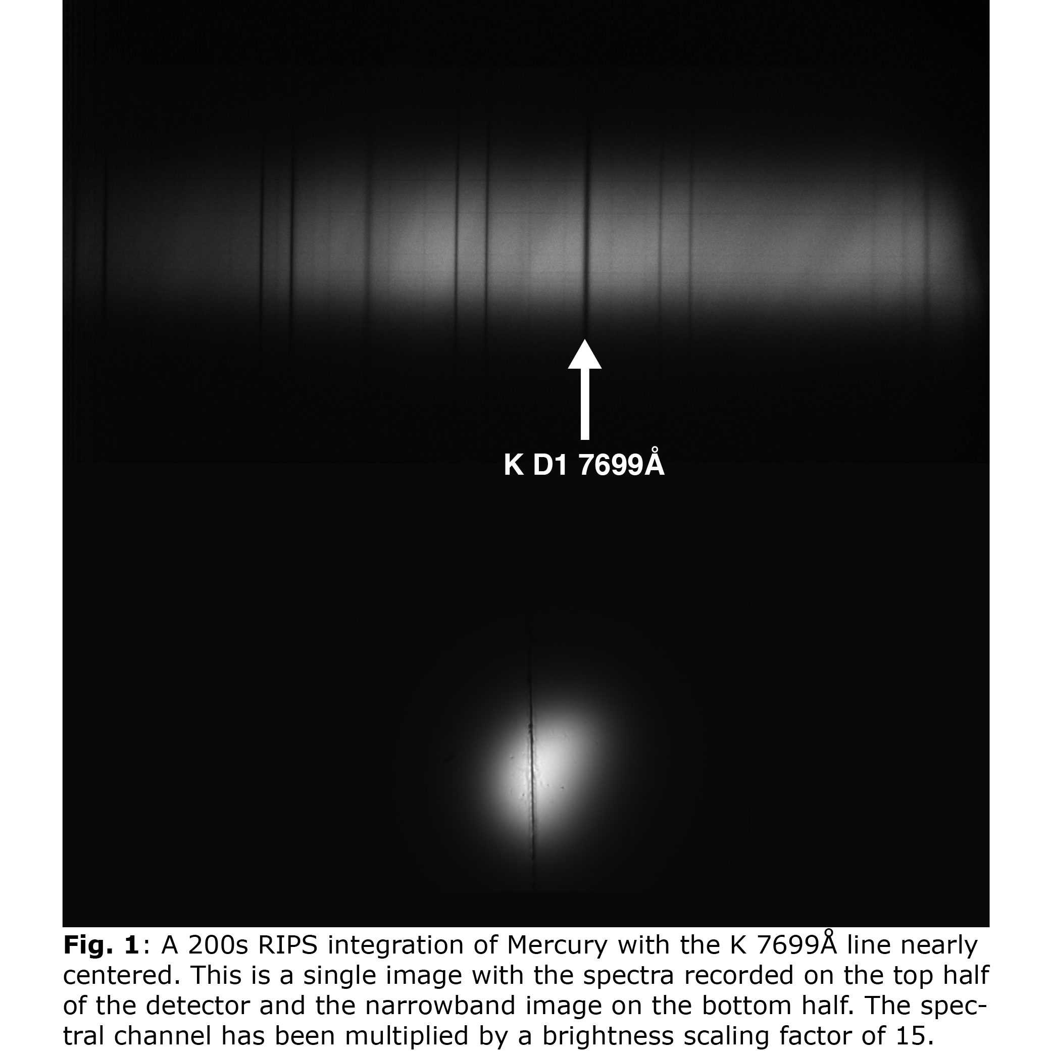
K observations were performed with the Rapid Imaging Planetary Spectrograph (RIPS) at the 3.67m Advanced Electro Optical System Telescope (AEOS) at Haleakala in 2018. The data we analyze here consist of 5 observations with integration times of 100 to 200 seconds, where the planet’s image is stabilized using adaptive optics. RIPS simultaneously records a narrowband image and a spectrum on a single CCD using mirrored slit jaws. The imaging channel provides both spatial registration of the slit aperture across the planet’s disk and a reference for the atmospheric blurring so that absolute brightness can be calibrated in each frame. Fig. 1 shows a 200s frame with the spectral channel brightness multiplied by 15 for visibility. Continuing with Mercury as its target, RIPS will provide dedicated ground support for the BepiColombo mission.
Analysis:
After standard dark and flat corrections, a photometric model is spatially convolved with a kernel and matched to RIPS’ imaging channel in order to determine the atmospheric and optical blurring unique to each observation. This reference for absolute flux and image quality is critical for observations at very high airmass. We apply a basic Hapke formulation [8] with parameters determined from MESSENGER’s Mercury Dual Imaging System [9]. The rotation and location of Mercury’s disk on RIPS’ detector, as well as an estimate for the seeing, are extracted by matching the imaging channel and photometric model. The result determines the absolute flux of Mercury’s continuum in units of MegaRayleighs per angstrom along the slit-length of the spectral channel.
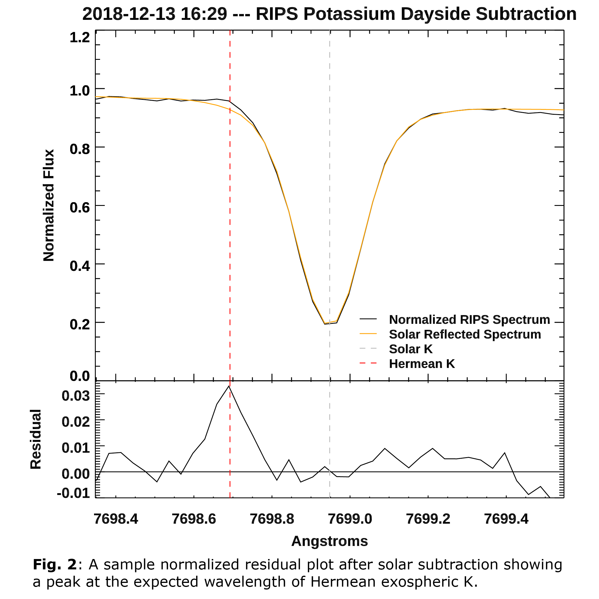
The recorded spectrum is rectified and normalized to the theoretical flux of the continuum. The spectrum is then spatially binned across Mercury’s disk. We found that five bins best optimized signal-to-noise ratio while preserving spatial information. The continuum is fit and subtraction is performed using a solar model [10]. This produces a residual signal of exospheric K seen in Fig. 2, which is integrated to obtain the binned brightness.
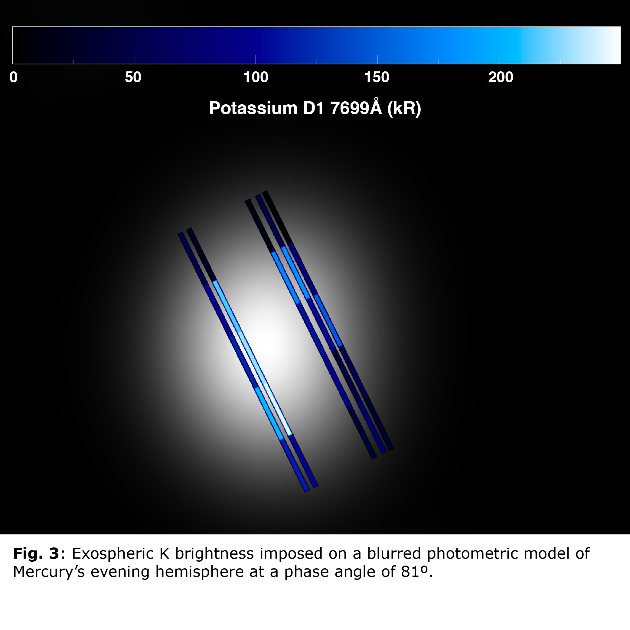
Results:
Fig. 3 shows the potassium emission in five discrete slit positions across Mercury’s disk imposed on a photometric model blurred to the average of the individual frames. The brightest calculated value for K is 250 kiloRayleighs, with the lowest being 3 kR. The mapped data suggest polar enhancement, particularly in the south. Enhancement over the southern cusp is characteristic of Mercury’s Na exosphere [4], but more data need to be analyzed to support this claim for K. Standard “g-value” calculations of the K excitation rate by solar photons allows this absolute brightness to be converted to column density. The peak column density corresponding to 250 kR is 4.1 × 109 cm-2. Local densities may be higher if the emitting region is unresolved. This column, together with previous RIPS results for Na D1+D2 abundance [4], results in an estimate of the Na to K ratio in the Hermean exosphere of about 25. This value is smaller than disk-averaged ratios in Potter et al. [5] (Na/K~ 34 to 142), or the range of spatial variations in the ratio that Doressoundiram et al. [7] reported (Na/K~ 80 to 400), but lies within the lower range reported by Killen et al. [6] (Na/K~ 22 to 49) across the planet’s dayside. The ratio calculated here should be interpreted cautiously since, while this estimate represents Na and K measurements from the same technique, these species were not observed concurrently, and alkali emissions are known to vary temporally.
References:
[1] Peplowski P. N. et al (2012) JGRE 117, E00L10.
[2] Peplowski P. N et al (2014) Icarus 228, 86.
[3] Cassidy, T. A. et al (2016) GeoRL 43, 121.
[4] Schmidt, C. A. et al (2020) Planet. Sci. J. 1, 4.
[5] Potter, A. E. et al. (2002) J. Geophys. Res. 107, E6.
[6] Killen, R. M. et al. (2010) Icarus 209, 75.
[7] Doressoundiram, A. et al. (2010) Icarus 207, 1.
[8] Hapke, B. (2012) Theory of Reflectance and Emittance Spectroscopy 2nd ed. (Cambridge: Cambridge Univ. Press).
[9] Domingue, D. L et al (2016) Icarus 268, 172.
[10] Kurucz, R. L. (2005) http://kurucz.harvard.edu/sun.html.
How to cite: Lierle, P., Schmidt, C., Baumgardner, J., Moore, L., and Swindle, R.: The Brightness of Mercury's Potassium Exosphere, Europlanet Science Congress 2020, online, 21 Sep–9 Oct 2020, EPSC2020-493, https://doi.org/10.5194/epsc2020-493, 2020.
We consider the possibility of radiation belts existence near Mercury. The study is carried out both using the Størmer theory for charged particles motion, in which zones of allowed and forbidden motion in an axially symmetric magnetic field are considered, and trajectories analysis.
The internal magnetic field of Mercury was discovered in 1974 by the Mariner 10 spacecraft. In [1] values for the dipole field at the Mercury equator Beq=192 nT and the north offset of the dipole dz=0.18 RM (where RM=2439 km is Mercury radius) were obtained, which were subsequently confirmed during the MESSENGER spacecraft flybys in 2011–2015. In our work, we also introduced a formal magnetopause at the distance Rmp=1.4 RM.
Allowed zones of particle motion are described in the Størmer theory in cylindrical coordinates by the inequality:
Q = 1 – (Pφ/(pρ) – qAφ/(pc))2 ≥0,
where Pφ is particle generalized angular momentum, p is its momentum, q is its charge, c is the speed of light, and Aφ is magnetic field vector potential (for more details see [2]). Equality Q=0 defines the boundaries of allowed zones, and Q=1 is a force line equation. We consider such Aφ, which is the sum of the potentials of pure dipole field and uniform external field be directing along the z-axis and approximating magnetopause currents fields.
Further, we measure lengths in units of the Størmer radius rst=√(qM/(pc)), where M is the absolute value of dipole magnetic moment. This radius acts as a scale factor. In a pure dipole field, it determines the curvature radius of the unstable circular trajectory lying in the dipole equatorial plane. The second Størmer integral of motion, arising as a result of axial symmetry, is the dimensionless parameter γ=Pφ/(2prst), which defines the shape and size (in rst) of allowed and forbidden zones. After their substitution, the inequality for Q takes the form:
Q = 1 – (2γ/ρ – ρ/r3 – Gρ)2 ≥0,
where we introduce a coefficient G=berst3/(2BeqRM3). In a pure dipole field for γ>1, there are two allowed zones: the infinite external and internal that is isolated and enclosed in the inner part of the sphere with radius rst. For external homogeneous field, in our calculations we used the value be=50 nT, whence G=–4.2717. In this case, when γ>–1/(8G) there is also a closed in space internal allowed zone.
Let us consider the motion of nonrelativistic particles, specifically protons, which trajectories start in points located at the dipole equatorial plane. Then an analysis based on Størmer’s theory can be connected with the classical description of particle motion through the initial pitch angle αeq and phase angle χeq as follows:
γ = 0.5 (1/R + R sin αeq sin χeq + R2G),
where R is the initial distance from the dipole.
On one hand, the condition of an internal allowed zone appearance from under the planet’s surface (that is possible, if rst is greater then planet radius), which occurs when γ=γin, must be fulfilled. On the other hand, the trajectories should not go beyond the magnetopause. The internal allowed zone firstly touches the magnetopause at γ=γout, and the final disappearance of the captured trajectories occurs at γfin<γout. As a consequence, in the case of Mercury only capturing of particles with kinetic energy K less than a few hundred keV can be possible. Particles within the internal allowed zone oscillate between mirror points, the positions of which depend on their initial pitch angles. Capturing of a particle possible if its mirror points is located above the planet’s surface, and the imprecision of the conservation of the 1st adiabatic invariant sin2α/B=const [3] does not lead to their significant displacement within the time T of interest to us. The description of the capture region located in the vicinity of the plane of the magnetic equator can be pictorially expressed by the formula:

where each elementary trajectory ‘traj.’ lies inside the allowed zone, α0 is αeq for the start position on the base of field line Q=1, αth1 and αth2 are the threshold values of α0 (Fig. 1), that as well as γfin slightly depend from T. Taking into account the variability of the Mercury magnetosphere, we chose prolonged T=20 minutes.

We considered sets of trajectories of 3∗104 protons with K=100 keV, the starting point of which was located at different distances R. Their motion was examined over a time interval of 60 seconds, in two directions in time. A particle that was thus captured for more than 2 minutes, which is approximately three times larger then their period of drift motion, was considered as captured (see Table).
| R (RM) | percentage of captured particles |
| 1.10 | 19.6 |
| 1.15 | 25.2 |
| 1.20 | 19.0 |
| 1.25 | 16.7 |
| 1.30 | 13.8 |
| 1.35 | 9.6 |
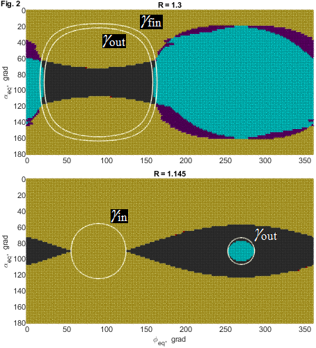
To describe the situation at the different points R, we also calculated maps showing the dependence of particles history on their initial pitch and phase angles (Fig. 2). Yellow color denotes particles colliding with the planet’s surface both in the past and in the future; red—either in the past or in the future; dark gray—capturing in the period under review; purple—arriving from outside the magnetopause and colliding with the surface, or vice versa; blue—flying by. We also drew the isolines γin, γout and γfin on these maps. As it can be seen, the flow of particles at a given point in the magnetosphere of Mercury does not consist solely of trapped, precipitated, or transit particles. At the same point, both passing particles and particles making less than one drift revolution before a collision with the planet surface can be detected.
[1] Alexeev I.I., Belenkaya E.S., Bobrovnikov S.Yu. et al. // J. Geophys. Res. Space Physics. 2008. V. 113. A12210.
[2] Lavrukhin A.S., Alexeev I.I., Tyutin I.V. // Ann. Geophys. 2019. V. 37. P. 535–547.
[3] Kuznetsov S.N., Yushkov B.Yu. // Plasma Physics Reports. 2002. V. 28, No. 4, pp. 342–350.
How to cite: Lukashenko, A., Lavrukhin, A., Alexeev, I., and Belenkaya, E.: A possibility to exist the trapped energetic particles zone near Mercury, Europlanet Science Congress 2020, online, 21 Sep–9 Oct 2020, EPSC2020-735, https://doi.org/10.5194/epsc2020-735, 2020.
The THEMIS solar telescope operating on Tenerife (Canary islands) has observed Mercury’s Na exosphere along several campaigns since 2007. A dataset of images taken between 2009 and 2013 are analysed here in relation with propagated solar wind data. A small subset of the images shows a low level of correlation between Na-emission and solar wind dynamic pressure. The amount of data at present is not sufficient to make a clear statement on whether the correlation is a coincidence or can be explained by other factors (position of Mercury and Earth, solar activity, etc.). Nevertheless, the authors present a comprehensive study taking into account all possible factors.
Sodium plays a special role in Mercury’s exosphere: due to its strong resonance line it has been observed and monitored by Earth-based telescopes for decades. Different and highly variable patterns of Na-emission have been identified, the most common and recurrent being the high latitude double-peak pattern [1]. It is clear that the exosphere is linked to the surface and influenced by the interstellar medium and the solar wind deviated by the magnetosphere, but the role and weight of the single processes are still under discussion [2].
In addition to the surface release processes already studied extensively in the past, we aim here to investigate more in detail the effect on Na exosphere of the following factors: the distance to the Sun, position in relation to the ecliptic plane, rotation of Mercury, solar UV and X-ray radiation. Na-emission intensity data (maximum and average) are provided by the dataset images collected from 2009 to 2013 by Earth-based observations performed at the THEMIS solar telescope.
In order to better investigate this open issue, we have studied the intensity of Na-emission as a function of solar wind dynamic pressure and true anomaly angle (TAA) of Mercury.
2.1 Propagated solar wind data
The present Na exosphere database can take advantage of the MESSENGER in-situ measurements of interplanetary magnetic field during the years 2011-2013. Unfortunately, the MESSENGER spacecraft had no in-situ measurement of solar wind parameters (velocity and density), so it is hard to interpret measurements that heavily depend on space weather circumstances. In order to overcome this difficulty, solar wind parameters from other space probes were shifted (in time and in space) with the Magnetic Lasso method to the position of Mercury [3]. Data of either the ACE or one of the two STEREO spacecraft were used, depending on which spacecraft had a smaller angular distance from Mercury.
All Na-emission images taken between 2009 and 2013 during relatively calm periods of the Sun were analysed, with a special focus on periods lasting for 2-3 consecutive days. Ten single cases are shown, in three cases there seems to be a direct (though not strong) relationship between solar wind pressure and emission intensity of Mercury’s Na-exosphere. A quantitative comparison is also carried out including a series of cases and the cross-correlation of several other factors with the aim to find the reason why the 3 selected cases show a higher correlation rate than the rest of the database.[a1] [M2]
The research of Mercury’s Na-emission variability is extended by the unknown solar wind dynamic pressure factor with the goal of reaching a more comprehensive understanding of exospheric processes occurring at the planet. Propagated solar wind parameters were used and compared with emission intensity. The study shows cases with a clear link between the two parameters.
Acknowledgements
We acknowledge use of NASA/GSFCʼs Space Physics Data Facilityʼs OMNIWeb (or CDAWeb or ftp) service, and OMNI data. We also thank the ACE SWICS instrument team and the ACE Science Center for providing the ACE data, NASA/NSSDC for Messenger data. MESSENGER data analysis was performed with the AMDA science analysis system provided by the Centre de Données de la Physique des Plasmas supported by CNRS, CNES, Observatoire de Paris and Université Paul Sabatier, Toulouse. We finally acknowledge the THEMIS staff in Tenerife (Canary Islands, Spain) for their fruitful help throughout the years of observation campaign. THEMIS data in 2013 was financially supported by the European Union's Horizon 2020 research and innovation program under grant agreement N. 824135 (SOLARNET). This work was partially supported by the OTKA FK128548 research grant.
References
[1] Mangano, V., Massetti, S., Milillo, A., Plainaki, C., Orsini, S., Rispoli, R., Leblanc, F.: THEMIS Na exosphere observations of Mercury and their correlation with in-situ magnetic field measurements by MESSENGER, Planetary and Space Science,115, 102–109,2015.
[2] Milillo, A.,Wurz, P., Orsini, S., Delcourt, D., Kallio, E., Killen, R.M., Lammer, H., Massetti, S., Mura, A., Barabash, A., Cremonese, G., Daglis, I.A., De Angelis, E., DiLellis, A.M., Livi, S., Mangano, V., Torkar, K.: Surface-exosphere-magnetosphere system of Mercury, Space Science Reviews, 117:397-443, 2005.
[3] Dósa, M., Opitz, A., Dálya, Z., Szegő, K.: Magnetic lasso: a new kinematic solar wind propagation method, Solar Physics 293:127,2018
How to cite: Dósa, M., Mangano, V., Bebesi, Z., Massetti, S., Milillo, A., and Görgei, A.: THEMIS telescope images analysed for space weather traces, Europlanet Science Congress 2020, online, 21 Sep–9 Oct 2020, EPSC2020-1022, https://doi.org/10.5194/epsc2020-1022, 2020.
The magnetosphere of Mercury is rather small and highly dynamic, due to its weak internal magnetic field and its close proximity to the Sun. The changing solar wind conditions principally determine the locations of both the Hermean bow shock and magnetopause. In 2011 – 2015 MESSENGER spacecraft completed more than 4000 orbits around Mercury, thus giving a data of more than 8000 crossings of bow shock and magnetopause of the planet. This makes it possible to study in detail the bow shock, the magnetopause and the magnetosheath structures.
In this work, we determine crossings of the bow shock and the magnetopause of Mercury by applying machine learning methods to the MESSENGER magnetometer data. We try to identify the crossings for the complete orbital mission and model the average three-dimensional shape of these boundaries depending on the external interplanetary magnetic field (IMF). Further, we try to clarify the dependence of the two boundary locations on the heliocentric distance of Mercury and on the solar activity cycle phase. Also, we study the effect of the IMF partial penetration into the Hermean magnetosphere. The results are compared with the obtained previously in other works.
This work may be of interest for future Mercury research related to the BepiColombo spacecraft mission, which will enter the orbit around the planet at December 2025.
How to cite: Lavrukhin, A., Parunakian, D., Nevskiy, D., Amerstorfer, U., Windisch, A., Julka, S., Möstl, C., Reiss, M., and Bailey, R.: Automatic detection of magnetopause and bow shock crossing signatures in MESSENGER magnetometer data, Europlanet Science Congress 2020, online, 21 Sep–9 Oct 2020, EPSC2020-826, https://doi.org/10.5194/epsc2020-826, 2020.
Origin and dynamical evolution of Mercury during the early stage of planet formation are still poorly understood (e.g., Ebel and Stewart, 2018, and references therein). Regardless of a scenario of Mercury’s formation, leftover planetesimals, asteroids, and comets would inevitably bombard Mercury’s surface after the completion of the primary accretion, including core-mantle separation. Such late impact bombardment is often called late accretion. The timing, duration and the dominant source (impactors’ origin) of late accretion to a terrestrial planet vary from model to model of planet formation (e.g., Abramov et al. 2013; Morbidelli et al. 2012; Morbidelli et al. 2018; Mojzsis et al. 2018; Brasser et al. 2020).
During late accretion, numerous small bodies impact on the surface of terrestrial planets – we define such impacts as cratering impacts. Late accretion would be a key process to characterize surface geomorphic and geochemical features of Mercury at the very last stage of its formation through global cratering, crust erosion, and accretion of exogenic impactors’ materials. Existing dynamical models indicate that Mercury experienced an impact bombardment with a total mass ranging from Mimp,tot ~ 0.08 × 10²⁰ to 8 × 10²⁰ kg (e.g., Abramov et al. 2013; Mojzsis et al. 2018; Brasser et al. 2020) and with impact velocity from vimp ~ 30 to 40 km/s (e.g., Le Feuvre and Wieczorek, 2008). However, the fate of the impactors and their effects on Mercury’s surface through the bombardment are still not clear.
Outcomes of cratering, surface erosion, and accretion of impactor’s material strongly depend on impact conditions (impact velocity, impact angle, and size of impactor). Recently, Hyodo & Genda (2020) derived scaling laws of erosion mass of target material and accretion mass of impactor material upon cratering impacts as a function of impact velocity and impact angle in a unit of impactor’s mass. In this work, by using these scaling laws (Hyodo & Genda 2020) as well as those predict the size of craters upon cratering impacts (e.g., Melosh and Vickery, 1989), we aim to understand the degree of global cratering, crustal erosion, and accretion mass of impactor materials during late accretion to Mercury.
Here, we attempt not to prioritize any specific scenario for late accretion (i.e., planet formation models). Instead, using Monte-Carlo and semi-analytical approaches combined with the scaling laws, we aim to generalize the outcomes of late accretion as a function of the total mass of impactors and typical impact velocity to Mercury (Hyodo et al. 2020, under review).
Within the range of parameters of late accretion discussed above as reference values, we report that late accretion could remove, on average, 50 m to 10 km of the primitive crust of Mercury. The cratering process during late accretion is extensive for erasing the older geological surface records on Mercury (see also, Mojzsis et al. 2018). Our Monte-Carlo simulations indicate that about 40 to 50wt.% of the impactor’s exogenic materials – about 0.3 × 10¹⁹ to 1.6 × 10¹⁹ kg in total including a consideration that accreted impactors’ material could be re-ejected during successive cratering impacts – are heterogeneously implanted on Mercury’s surface during late accretion. About half of the accreted impactor’s materials would be vaporized and the rest would be completely melted. We expect that our results would be useful to bridge predictions of different planet formation models and the detailed surface observations of Mercury, including the BepiColombo mission (Hyodo, Genda & Brasser 2020, under review).
How to cite: Hyodo, R., Genda, H., and Brasser, R.: Late accretion to Mercury: Global cratering, crust erosion, and accretion of exogenic materials, Europlanet Science Congress 2020, online, 21 Sep–9 Oct 2020, EPSC2020-487, https://doi.org/10.5194/epsc2020-487, 2020.
Please decide on your access
Please use the buttons below to download the presentation materials or to visit the external website where the presentation is linked. Regarding the external link, please note that Copernicus Meetings cannot accept any liability for the content and the website you will visit.
Forward to presentation link
You are going to open an external link to the presentation as indicated by the authors. Copernicus Meetings cannot accept any liability for the content and the website you will visit.
We are sorry, but presentations are only available for users who registered for the conference. Thank you.