OPS2 | Jupiter and Giant Planet Systems: Juno Results

OPS2

Jupiter and Giant Planet Systems: Juno Results
Co-organized by TP/EXOA
Convener: Scott Bolton | Co-conveners: Francesca Zambon, Heidi Becker, Anton Ermakov, Paul Hartogh, Alessandro Moirano, Ali Sulaiman
Orals
| Mon, 09 Sep, 08:30–12:00 (CEST), 14:30–16:00 (CEST)|Room Sun (Auditorium)
Posters
| Attendance Tue, 10 Sep, 10:30–12:00 (CEST) | Display Tue, 10 Sep, 08:30–19:00, Attendance 14:30–16:00 (CEST) | Display Tue, 10 Sep, 08:30–19:00
Orals |
Mon, 08:30
Tue, 10:30
The Juno spacecraft continues its journey around Jupiter and its satellites making new important discoveries. Results from Juno at Jupiter have revealed numerous processes associated with the physics and chemistry of its interior, atmosphere, magnetosphere and its origin and evolution. Juno’s extended mission transformed the Jupiter-focused mission to a full system explorer. The extended mission runs through 2025 and includes numerous close and distant flybys of Io, Europa, and Ganymede along with an exploration of Jupiter’s enigmatic ring system. This session invites observational and modeling results related to Juno’s results on Jupiter and the comparison to other giant planets and exo-planetary systems. New results from Juno’s extended mission on Jupiter’s northern latitudes as well as the satellites and ring system are welcome.

Orals: Mon, 9 Sep | Room Sun (Auditorium)

Chairpersons: Scott Bolton, Alessandro Mura
08:30–08:45
|
EPSC2024-512
|
solicited
|
On-site presentation
Vincent Hue, Thibault Cavalié, James A. Sinclair, Xi Zhang, Bilal Benmahi, Pablo Rodríguez-Ovalle, Rohini S. Giles, Tom S. Stallard, Rosie E. Johnson, Michel Dobrijevic, Thierry Fouchet, Thomas K. Greathouse, Denis C. Grodent, Ricardo Hueso, Olivier Mousis, and Conor A. Nixon

Jupiter's polar stratosphere exhibits unique chemical and dynamical processes that shape its atmospheric composition and structure. This paper reviews observational constraints and modeling efforts aimed at understanding the complex interplay between chemistry, dynamics, and aerosol microphysics in Jupiter's high-latitude regions.

Hydrocarbon observations from various instruments (e.g. Voyager/IRIS, Cassini/CIRS, IRTF/TEXES, Juno/UVS, and JWST/MIRI) have revealed significant abundance enhancements and latitudinal variations of species like acetylene (C2H2), ethylene (C2H4), ethane (C2H6), methylacetylene (CH3C2H), and benzene (C6H6) within the auroral regions. These enhancements are attributed to the influence of auroral processes and possible enhanced vertical mixing. IRTF/TEXES and JWST/MIRI also provided insights into the vertical structure of the polar atmosphere, suggesting that the methane homopause (i.e. the altitude where the methane molecular diffusion coefficient equals the vertical eddy diffusion one, and above which CH4 abundance decreases due to the molecular diffusion), is located at higher altitudes within the auroral regions compared to lower latitudes. Some of these observations also indicate that the aerosol layer is located at higher altitudes (above 20 mbar) in the polar regions compared to lower latitudes (around 50 mbar).

Modeling efforts have aimed to reproduce the observed meridional distributions of hydrocarbons and constrain the atmospheric dynamics and transport processes. 2D photochemical modeling, with parametrized meridional diffusion coefficients (Kyy) and advective circulation, suggests that a combination of moderate Kyy and a circulation cell with upwelling motions at the equator and downwelling motions at mid-latitudes is required to reproduce the observed meridional gradient of ethane (C2H6). Auroral chemistry models have explored the production of larger hydrocarbon ions and neutral species through ion-neutral reactions initiated by precipitating auroral particles, highlighting the potential role of auroral processes in the formation of stratospheric haze.

Cassini and ALMA observations of hydrogen cyanide (HCN) have revealed a striking enhancement and distinct vertical distribution within the auroral regions compared to lower latitudes, suggesting the influence of atmospheric dynamics on the chemical distributions. Measurements of the Doppler shifts in H3+ emission lines from ground-based telescopes, combined with measurements of wind-induced Doppler shifted HCN lines from ALMA, have revealed the presence of strong upper-atmospheric winds circulating around Jupiter's polar regions, possibly influencing the circulation down to the middle stratosphere.

Recent observations and modeling efforts have advanced our understanding of Jupiter's polar stratosphere. Key findings include the enhancement of hydrocarbon abundances within auroral regions, the higher altitude of the methane homopause and aerosol layers in polar regions, and the interplay between chemistry, dynamics, and aerosol microphysics in shaping the atmospheric composition and structure. We summarize the remaining outstanding questions that are to be addressed by current as well as forthcoming facilities and space missions.

Figure 1: Summary schematics of selected chemical distributions across Jupiter’s polar region. Particle precipitation leads to the formation of H3+ in the ionosphere, and to UV-auroras through the H and H2 emissions at the μbar level. Around the μbar level and below, solar-UV photolysis as well as charged particle precipitation leads to the formation of hydrocarbons. As hydrocarbons diffuse downward, they combine into heavier hydrocarbons and eventually form aerosols. HCN produced in the upper atmosphere, possibly from N2 destruction, becomes incorporated into aerosols before reaching ∼2mbar or below.

How to cite: Hue, V., Cavalié, T., Sinclair, J. A., Zhang, X., Benmahi, B., Rodríguez-Ovalle, P., Giles, R. S., Stallard, T. S., Johnson, R. E., Dobrijevic, M., Fouchet, T., Greathouse, T. K., Grodent, D. C., Hueso, R., Mousis, O., and Nixon, C. A.: The Polar Stratosphere of Jupiter, Europlanet Science Congress 2024, Berlin, Germany, 8–13 Sep 2024, EPSC2024-512, https://doi.org/10.5194/epsc2024-512, 2024.

08:45–09:00
|
EPSC2024-866
|
ECP
|
solicited
|
On-site presentation
Maria Smirnova, Eli Galanti, Andrea Caruso, Dustin Buccino, Luis Antonio Gomez Casajus, Edoardo Gramigna, Marco Zannoni, Marzia Parisi, Bill Hubbard, Paul Steffes, Steven Levin, Scott Bolton, Paolo Tortora, and Yohai Kaspi

The shallow layers of the Jovian atmosphere, the only regions accessible to direct investigation through in situ sampling and remote sensing experiments, are the looking glass through which the unknowns of Jupiter's structure are revealed. Radio occultation experiments have proved to offer invaluable opportunities to investigate the atmospheric dynamics of Jupiter, akin to descending a probe into its upper layers, offering unique insights into the thermal structure and composition.

Since July 2023, Juno's extended mission has presented a multitude of such opportunities, with each passing month bringing forth a new experiment, a first since the Voyager missions. In these experiments, as the Juno spacecraft orbits Jupiter, it is obscured by the planet along its trajectory. As the electromagnetic signal from the spacecraft travels towards Earth, it traverses through Jupiter's atmosphere, resulting in refraction on the signal. This refraction is recorded on the ground station as a frequency shift, known as the Doppler shift, compared to its expected frequency in a vacuum environment. Radio occultation experiments capitalize on these refraction effects to investigate and decipher the atmospheric vertical properties of the planetary atmosphere up to 0.5 bar.

The Juno radio occultations of Jupiter operated in a coherent two-way mode, utilizing multi-frequency link signals. Consequently, this study necessitated the use of an optimization method employing ray tracing techniques to track both the uplink and downlink signal through the neutral atmosphere in X- and Ka-band, enabling the extraction of vertical profiles of atmospheric parameters. The analyzed atmospheric pressure-temperature profiles highlight the potential of Juno's radio occultation experiments in elucidating the relatively unknown neutral atmosphere of Jupiter. In this presentation we present initial results from Juno's first year of radio occultations, analyse the measurement sensitivity concerning density and temperature, investigate the vertical temperature profiles at different latitudes and discuss their implications regarding the dynamics of Jupiter.

How to cite: Smirnova, M., Galanti, E., Caruso, A., Buccino, D., Gomez Casajus, L. A., Gramigna, E., Zannoni, M., Parisi, M., Hubbard, B., Steffes, P., Levin, S., Bolton, S., Tortora, P., and Kaspi, Y.: Analysis of Jupiter's atmosphere using Juno's radio occultations, Europlanet Science Congress 2024, Berlin, Germany, 8–13 Sep 2024, EPSC2024-866, https://doi.org/10.5194/epsc2024-866, 2024.

09:00–09:10
|
EPSC2024-734
|
ECP
|
On-site presentation
Simon Müller and Ravit Helled

Updated formation and structure models of Jupiter predict a metal-poor envelope. This is at odds with the two to three times solar metallicity measured by the Galileo probe. Additionally, Juno data imply that water and ammonia are enriched. This talk explores whether Jupiter can have a deep radiative layer separating the atmosphere from the deeper interior. The radiative layer could be caused by a hydrogen-transparency window or depletion of alkali metals.

We show that heavy-element accretion during Jupiter's evolution can lead to the desired atmospheric enrichment and that this configuration is stable over billions of years. The origin of the heavy elements could be cumulative small impacts or one large impact. The preferred scenario requires a deep radiative zone due to a local reduction of the opacity at ∼ 2000 K by ∼ 90%, which is supported by Juno data, and vertical mixing through the boundary with a similar efficiency to molecular diffusion (D ≤ 10-2 cm2/s). Most of Jupiter's molecular envelope could have solar composition while its uppermost atmosphere is enriched with heavier elements. The enrichment likely originates from the accretion of solid objects.

This possibility resolves the long-standing mismatch between Jupiter's interior models and atmospheric composition measurements. Furthermore, our results imply that the measured atmospheric composition of exoplanets does not necessarily reflect their bulk compositions. We also investigate whether the enrichment could be due to the erosion of a dilute core and show that this is highly unlikely. The core-erosion scenario is inconsistent with evolution calculations, the deep radiative layer, and published interior models.

How to cite: Müller, S. and Helled, R.: Can Jupiter's atmospheric metallicity be different from the deep interior?, Europlanet Science Congress 2024, Berlin, Germany, 8–13 Sep 2024, EPSC2024-734, https://doi.org/10.5194/epsc2024-734, 2024.

09:10–09:15
09:15–09:25
|
EPSC2024-553
|
On-site presentation
Ingo Müller-Wodarg, Peio Iñurrigarro Rodriguez, Luke Moore, Alexander Medvedev, and Tommi Koskinen

Jupiter’s upper atmosphere (thermosphere/ionosphere) forms the link between its deeper atmosphere and the vast magnetosphere with its current systems, some of which close in the planet’s auroral region. The combination of acceleration and heating have profound influence on the dynamics and temperatures of Jupiter’s upper atmosphere. The ongoing Juno and future JUICE missions as well as Earth based observations provide us with new measurements and questions about the upper atmosphere structure and dynamics. Fundamentally, the aim is to understand this highly coupled upper atmosphere region which is driven to varying degrees by the magnetosphere and by the deeper atmosphere via vertically propagating waves.

Exploring such a complex system requires global numerical models. Based on our Saturn Thermosphere Ionosphere Model (STIM) [1, 2, 3], we have developed a Jupiter Thermosphere Ionosphere Model (JTIM) which includes similar features as STIM, a thermosphere model coupled chemically and dynamically to an ionosphere model. The code numerically solves the coupled non-linear Navier Stokes equations of momentum, energy and continuity, including eddy and molecular diffusion of neutral gases and full two-way ion-neutral coupling. The magnetosphere interaction is currently accounted for by mapping a magnetospheric electric field and precipitation pattern into the polar regions and allowing for particle impact ionization in the auroral regions. The thermosphere’s lower boundary is flexible to allow for coupling to the deeper atmosphere via mean background parameters and atmospheric waves.

We present first simulations of the model with a focus on the complex thermosphere dynamics and thermal structure. The use of similar models for both Saturn and Jupiter allows for direct comparisons between the planets and difference in underlying physical processes under differing boundary conditions. We also address the question of the well-known upper atmosphere temperature conundrum which is common to all giant planets in our solar system.


References:

[1] Müller-Wodarg et al. A global circulation model of Saturn’s thermosphere. Icarus, 180, 2006.

[2] Müller-Wodarg et al. Magnetosphere-atmosphere coupling at Saturn: 1 – Response of thermosphere and ionosphere to steady state polar forcing. Icarus, 221, 2012.

[3] Müller-Wodarg et al. Atmospheric Waves and Their Possible Effect on the Thermal Structure of Saturn's Thermosphere. Geophysical Research Letters, 46, 2019.

How to cite: Müller-Wodarg, I., Iñurrigarro Rodriguez, P., Moore, L., Medvedev, A., and Koskinen, T.: Dynamics and thermal structure of Jupiter’s thermosphere in response to magnetosphere-atmosphere coupling, Europlanet Science Congress 2024, Berlin, Germany, 8–13 Sep 2024, EPSC2024-553, https://doi.org/10.5194/epsc2024-553, 2024.

09:25–09:35
|
EPSC2024-378
|
On-site presentation
John Rogers, Candice Hansen, Gerald Eichstädt, Glenn Orton, Tom Momary, Gianluigi Adamoli, Robert Bullen, Michel Jacquesson, Marco Vedovato, and Hans-Jörg Mettig

By combining data from JunoCam and ground-based images, we present a history of the large-scale cyclonic structures in Jupiter’s S2 domain spanning 7.5 years, thus establishing the range of lifetimes of chaotic formations for the first time. The S2 domain lies between the prograde jets at 36ºS (planetographic) and 43ºS, encompassing the traditionally named South South Temperate Belt (SSTB) and Zone (SSTZ).  The most distinctive features here are 6 to 9 long-lived anticyclonic white ovals (AWOs) [ref.1].  Between them are a number of cyclonic circulations, which have been well characterised by short-term imaging from previous spacecraft, but could not be comprehensively followed because many of them were not well resolved in ground-based images.  Images from JunoCam now enable most or all of them to be characterised on each of Juno’s orbits (e.g. Figure 1), and modern amateur imaging can resolve them more frequently for several months around Jupiter’s oppositions (e.g. Figure 2).  Thus we can now document these cyclonic features in the SSTB continuously from 2015 to 2023, along with high-resolution views of them from JunoCam.

They fall into three categories:  (i) Cyclonic dark spots or oblongs, often dark brown. (ii) Cylonic white oblongs (CWOs).  (iii) Folded filamentary regions (FFRs).

The first two are closed circulations; FFRs are more chaotic and may emit disturbance to east and west. The JunoCam images also sometimes reveal long, pale fawn-coloured sectors of the SSTB that resemble CWOs in structure and are probably closed circulations. In ground-based images these may appear as a dull-white CWO (because JunoCam is more sensitive to blue absorption than typical amateur filters) or as a nondescript sector of the SSTB. 

A diagrammatic chart showing the history of these types of cyclonic feature is in Figure 3.  Any of them can last for as little as ~4 months.  CWOs often last longer, ranging up to 2.8 years in this survey, and up to nearly 6 years in earlier ground-based records [ref.1].  FFRs also have a large range of lifetimes, although they may sometimes be temporarily weak; two have existed for the full duration of this survey (>7.5 years). Some sectors (delimited by AWOs) have shown repeated changes between the cyclonic types: any of three types can convert into any other over a matter of months, sometimes via a pale ochre oblong as intermediate (Figures 1 & 4).

Dark oblongs may form when a FFR becomes inactive.  Dark spots or oblongs often end their lives by becoming redder and then lighter in colour, sometimes becoming white.  Some of these dark spots are very small and can turn into white ovals that do not expand; these are not considered further here.  Longer structures can turn into light oblongs which expand in longitude as CWOs. 

CWOs sometimes brighten rapidly in their early stages; a new one in 2018 was very bright white and also bright in the 889-nm methane band, as was one in 2013 (just before this survey period).  This was not a transient convective plume, but static methane-brightness of the white oblong, which is a very rare condition for a cyclonic oval on Jupiter.  CWOs always expand in longitude during their lifetime. Four CWOs whose later stages were observed by JunoCam all ended gradually, changing from white to dull white or fawn, sometimes being very long but retaining the loop form suggesting continuing circulation; sometimes it was also visibly disturbed.  This stage lasted for up to a year; then in three cases it was terminated by a new FFR developing within its former boundaries.

New FFRs have appeared and disappeared about once a year.  A young FFR is usually small and expands, though they do not grow indefinitely.  We have never noted an especially bright convective outbreak initiating a FFR, though many could have gone undetected; and only one JunoCam observation of a young one showed it as methane-bright.

All three types are equivalent to cyclonic features in most other domains, although their relative size and importance vary. [See our abstract in the ODAA1 session for the STB.]  For example, dark spots or oblongs are smaller versions of ‘barges’ in the NEB; CWOs resemble structures in the STB; and FFRs are increasingly dominant in higher-latitude domains. This study is the first to show the full timecourse of FFRs.  Similar studies will be possible for other domains, in which the FFRs may be more variable and perhaps shorter-lived because they are not usually confined by AWOs.


Acknowledgements:  Some of this research was carried out at the Jet Propulsion Laboratory, California Institute of Technology, under a contract with the National Aeronautics and Space Administration (80NM0018D0004).

Details of the observations are posted in our regular reports on the JunoCam and BAA websites: 

https://www.missionjuno.swri.edu/junocam;  https://britastro.org/sections/jupiter


Reference 1:  Rogers J, Adamoli G, Hahn G, Jacquesson M, Vedovato M, & Mettig H-J (2014).  ‘Jupiter’s southern high-latitude domains: long-lived features and dynamics, 2001-2012.’ http://www.britastro.org/jupiter/sstemp2014.htm


Figure 1:

Figure 2:

Figure 3:

Figure 4:

How to cite: Rogers, J., Hansen, C., Eichstädt, G., Orton, G., Momary, T., Adamoli, G., Bullen, R., Jacquesson, M., Vedovato, M., and Mettig, H.-J.: Longevity of cyclonic formations in Jupiter’s S2 (South South Temperate) Domain, Europlanet Science Congress 2024, Berlin, Germany, 8–13 Sep 2024, EPSC2024-378, https://doi.org/10.5194/epsc2024-378, 2024.

09:35–09:45
|
EPSC2024-154
|
On-site presentation
Gerald Eichstädt, Shawn Brueshaber, Cheng Li, Glenn Orton, John Rogers, Candice Hansen-Koharcheck, and Scott Bolton

Introduction

Storms on Earth barely develop counter-rotating cores nor do so computer simulations of two-dimensional and incompressible Euler fluids [2]. But on Jupiter, JunoCam [1], the visible light imager on NASA's Juno spacecraft, collected image data of northern circumpolar cyclones (CPCs) that show distinct counter-rotating cores. Those cores occur either frequently, or they are often stable over several months.

The data points of our long-term time series are separated by the duration of at least one Juno orbit. Short-term image sequences taken during each of the considered Jupiter flybys reveal the morphology as well as the dynamics of a CPC.

While color images provide sufficient detail to measure angular velocities by stereo correspondence, and to derive vorticity maps, some of the methane-band image sequences reveal that counter-rotating cores do not stand out significantly. Two layers of clouds, one with a converging cyclonic flow, and one with a diverging anticyclonic flow, are not immediatley suggested by methane-band images. Therefore, a fluid-dynamical solution of counter-rotation within a two dimensional geometry ought to be found.

A counter-rotating core in a vortex of a two-dimensional Euler fluid is unstable. It is either ejected or disrupted in many cases.

Modelling a second layer, one with a steady flow, and allowing for some friction with the two-dimensional fluid of interest, can stabilize the counter-rotating core. The friction acts equivalently to vortex flux into or out of the layer of interest. The vortex flux is defined to be proportional to the difference between the vorticity fields of the two fluid layers, while the reference vorticity field remains constant. The global parameter of proportionality can be varied between 0 and 1, where 0 means no effect to the two-dimensional Euler fluid, and 1 means an identical copy of the steady flow. It's convenient to define the parameter of proportionality in terms the half-life of the vorticity flux in a sense that after that time, half of the vorticity difference would be leveled out in the absence of dynamics. A half-life of infinity translates into a parameter of proportionality of 0 for each simulation step, and a half-life of 0 translates into a parameter of proportionality of 1.

Vorticity maps and radial vorticity profiles in JunoCam images of CPCs

Figure 1

The first column of Figure 1 shows a northern CPC without a counter-rotating core. The angular velocity is increasing with decreasing distance from its center. The morphology shows a  typical spiral structure, the vorticity map shows a strongly cyclonic core, and the radial vorticity profile (blue line in the diagram) has its cyclonic maximum at the center of the cyclone (left end of the x-axis).

The two other columns show two CPCs with counter-rotating cores. The central column shows a gradual transition from cyclonic to anticyclonic rotation with decreasing radius, while the right colums shows a sharp boundary between the anticyclonic core and its cyclonic environment. In both cases, the radial vorticity profile shows an anticyclonic maximum at the center of the cyclone and a shallow local cyclonic maximum outside the center of the cyclone.

While an anticyclonic morphology can form for a cyclone with cyclonic vorticity decreasing towards the center, measurements of the dynamics return distinct anticyclonic rotation in the cores.

Long-term stability of anticyclonic cores

Figure 2

JunoCam observes the same CPC during several Jupiter flybys. Figure 2 shows such an example. The same CPC was observed during the PJ50, PJ51, PJ54, and PJ58 flybys. Each time, an anticyclonic morphology was detected at the core of the CPC. This means either that such a morphology developed with each flyby, or, more plausibly, lasted at least from PJ50 (2023 APR 08) to PJ58 (2024 FEB 03), hence for about ten months.

Methane-band images hint towards 2D embedding of the counter-rotation

Figure 3

The left column of Figure 3 shows a CPC with a cyclonic core, while the right column shows an example with a counter-rotating core. In both cases, color and methane-band images are available. The methane-band images do not show a significant difference between the relative elevation profiles of the two cyclones. With the cyclonic core assumed to be embedded in a 2D flow, this suggests that the same should be considered for the anticyclonic core.

Counter-rotating cores are unstable in an incompressible 2D Euler flow

Figure 4

Counter-rotating cores in an incompressible 2D Euler flow are usually either ejected or disrupted. Figure 4 visualizes time series of both scenarios. Bluish symbolizes cyclonic vorticity, and yellowish anticyclonic vorticity.

Vorticity flux by friction with a second layer stabilizes counter-rotation

Figure 5

Each row in Figure 5 represents a time series of the same 2D flow, but with varying levels of friction with a steady flow identical to the left-most column of the survey. The half-life of the vorticity flux increases from top to bottom. The top line approximates a steady flow with a stable counter-rotating core rather quickly, while the bottom line represents just the 2D Euler fluid without friction.

Conclusion

The counter-rotating core observed in Jupiter's northern CPCs suggest to exist in an approximately 2D fluid dynamical settings. Such a flow appears to be unstable for an incompressible 2D Euler flow. But for an appropriate vorticity exchange with a steady flow in a second 2D layer, the incompressible 2D Euler flow can be extended to a vortex with a stable counter-rotating core. The cause of the assumed steady flow in the second fluid level is out of the scope of this article.

Acknowledgement

Some of this research was carried out at the Jet Propulsion Laboratory, California Institute of Technology, under a contract with the National Aeronautics and Space Administration (80NM0018D0004).

References

[1] C.J. Hansen, M.A. Caplinger, A. Ingersoll, M.A. Ravine, E. Jensen, S. Bolton, G. Orton. Junocam: Juno’s Outreach Camera. Space Sci Rev 2013:475-506, 2017

[2] Eichstädt, G., Hansen, C., and Orton, G.: Fluid Dynamical 2D Simulations of Jupiter's South Polar Region Based On JunoCam Image Data, EGU General Assembly 2020, Online, 4–8 May 2020, EGU2020-12025, https://doi.org/10.5194/egusphere-egu2020-12025, 2020.

How to cite: Eichstädt, G., Brueshaber, S., Li, C., Orton, G., Rogers, J., Hansen-Koharcheck, C., and Bolton, S.: Counter-rotating cores in Jupiter's circum-polar cyclones observed by JunoCam and modeled in 2D, Europlanet Science Congress 2024, Berlin, Germany, 8–13 Sep 2024, EPSC2024-154, https://doi.org/10.5194/epsc2024-154, 2024.

09:45–09:55
|
EPSC2024-689
|
ECP
|
On-site presentation
Xing Cao, Peng Lu, Binbin Ni, and Shaobei Wang

Whistler-mode chorus waves are frequently observed in the Jovian magnetosphere and are known to play an important role in the dynamics of radiation belt electrons. By combining the observations from Galileo and Juno, we conducted a detailed statistical analysis of the spatial distribution of the occurrence rates, power spectral densities and averaged amplitudes of chorus waves in the Jovian magnetosphere. The statistical results show that chorus waves are mainly distributed in the near-equatorial (<20°) region at 5< M-shell <12. The averaged wave amplitudes range from several pT to tens of pT and are significantly enhanced in the vicinity of Europa and Ganymede. The wave amplitudes peak at M-shell = 8-11 within λ≤10° with a strong dawn-dusk asymmetry. In addition, the wave power spectral intensities decrease monotonically with increasing f/fce, where f and fce are the wave frequency and electron gyrofrequency, respectively. We subsequently construct an empirical model of the distribution of chorus wave amplitudes with M-shell, magnetic latitude and magnetic local time. Based on the developed wave model, we investigate the resonant interactions between chorus wave and radiation belt electrons at different M-shells. Our results improve the current understanding of the statistical distribution properties of chorus waves and their role in the dynamics of radiation belt electrons at Jupiter.

How to cite: Cao, X., Lu, P., Ni, B., and Wang, S.: Statistical distribution of chorus waves in the Jovian magnetosphere and their resonant interactions with radiation belt electrons, Europlanet Science Congress 2024, Berlin, Germany, 8–13 Sep 2024, EPSC2024-689, https://doi.org/10.5194/epsc2024-689, 2024.

09:55–10:00
Coffee break
Chairperson: Alessandro Moirano
10:30–10:45
|
EPSC2024-801
|
solicited
|
On-site presentation
Leigh N. Fletcher, Francesco Biagiotti, Oliver R.T. King, Michael T. Roman, Henrik Melin, Jake Harkett, Imke de Pater, Thierry Fouchet, Alessandro Mura, Davide Grassi, Guiseppe Piccioni, Mike Wong, Pablo Rodríguez-Ovalle, Patrick Irwin, Glenn Orton, Pat Fry, Gordy Bjoraker, and Ricardo Hueso

We present observations of Jupiter’s atmosphere using JWST’s NIRSpec (Jakobsen+2022, doi:10.1051/0004-6361/202142663) integral field unit (IFU) spectrometer acquired during the first year of scientific operations.  Near-infrared spectroscopic mapping provides a key tool for studying giant planet clouds, hazes, and gaseous composition from the cloud-forming weather layer to the radiatively-controlled lower stratosphere.  Spectrometers that span the 1-5 µm range provide access to reflected sunlight inside and outside of strong methane bands; ionospheric emission from H3+; and deep thermal emission from an atmospheric ‘window’ near 5 µm (where gaseous absorption is relatively low).  The superb spectral sensitivity, spectral resolution (R~2700), and uninterrupted spectral range of NIRSpec/IFU has provided an exquisite dataset for studying the 3D structure of Jupiter’s dynamic atmosphere, with sensitivity to wavelengths that have been previously inaccessible.  In this presentation, we compare NIRSpec/IFU spectra to those acquired by the JIRAM instrument (2-5 µm spectrometer) on NASA’s Juno spacecraft (Adriani+2017, doi:10.1007/s11214-014-0094-y), and look ahead to future Jupiter observations by the MAJIS instrument on JUICE (Poulet+2024, doi:10.1007/s11214-024-01057-2).

JWST Observations:  We used the NIRSpec/IFU instrument to acquire spatially-resolved spectral maps of Jupiter across a 3x3” field-of-view (FOV), using mosaicking to ensure wide spatial coverage.  Two gratings were used at high spectral resolution (R~2700, G235H and G395H) to span the 1.8-5.3 µm range.  While the small NIRSpec FOV precludes global mapping of Jupiter, representative regions of the atmosphere can be explored by combining multiple datasets.  As part of early-release science (ERS, PIs:  de Pater & Fouchet) programme 1373, six mosaic tiles were used to map the Great Red Spot on 2022-07-27 using both gratings; six G395H (2.8-5.3 µm) tiles and three G235H tiles (1.8-3.2 µm) were used to map Jupiter’s South Polar domain on 2022-12-27.  Data were reduced and navigated using the JWST pipeline and custom Solar System processing (King+2023, doi:10.3847/2515-5172/ad045f), mitigating the effects of saturation in reflectivity peaks near ~2 µm and strong thermal emission at 5 µm by subdividing long integrations into shorter durations (known as groups).  Emission features from H3+ and CH4 fluorescence were identified in the data (Melin+2024) and removed to enable fitting of the neutral atmosphere.

Great Red Spot:  JWST captured the GRS in July 2022 in a relatively quiescent state (Fig. 1), with fine tendrils of material (reddish in visible light) forming an anticlockwise spiral at the edge of the vortex, and cloud-free lanes of low reflectivity and bright thermal emission surrounding both the red anticyclone and the reflective aerosols of the GRS hollow.  Intriguingly, reflectivity maps between 3.0 and 4.5 µm (sounding upper-tropospheric aerosols) show a series of concentric ovals, forming lanes around the centre of the GRS, with the most reflective in the centre where wind speeds are lowest (and sometimes there is a counter-rotating cyclonic core).  A combination of principal component analysis (PCA) and Gaussian Mixture Models (GMM) was used to identify self-similar NIRSpec spectra (Biagiotti+2024, doi:10.5194/egusphere-egu24-12950), forming clusters for subsequent spectral inversion with NEMESIS to derive aerosol properties and gaseous abundances.  The clustering naturally identified the different spectra in the dark cloud-free regions; the whitish aerosols of the GRS hollow; and the red-orange aerosols of the GRS.  A persistent cluster defines the edge or halo of the GRS, showing a spectrum that is distinct from the GRS interior.  We repeated the same analysis on Juno/JIRAM spectra of the GRS acquired during Juno’s first perijove (2016-08-27, Grassi+2021, doi:10.1093/mnras/stab740), albeit with lower spectral resolution and coarser coverage of the JIRAM spectrometer.  The same clusters were identified, and the same persistent halo.  The halo may be associated with the mixture of red chromophores and the underlying background clouds. The clusters show considerable difference in the shape of the 2.6-2.8 µm reflectivity peak, indicating the presence of different cloud and haze properties (compositions, particle sizes, altitude distributions, etc.) in the different clusters.  Clusters closer to the GRS centre appear to have a distinct 2.7-µm reflectivity peak that is spectrally broader with enhanced reflection out beyond 3.0 µm.  Inversions varying the properties of the upper haze, deeper clouds, and abundances of ammonia and phosphine will be presented to determine the origin of the concentric lanes within the GRS.  Results will be compared to previous near-IR studies from Galileo/NIMS (Baines+2002, doi:10.1006/icar.2002.6901) and ground-based observations (Bjoraker+2018, doi:10.3847/1538-3881/aad186).

Figure 1 Jupiter's Great Red Spot observed by NIRpec at three wavelengths:  2.7 µm (reflection from deep clouds); 4.5 µm (combined reflection and thermal emission); and 4.6 µm (deep thermal emission).

South Polar Domain:  The December-2022 mosaic spans approximately 100o longitude (centred on ~20oW) and 50-90oS, with clearly-identifiable transitions in reflectivity and thermal emission associated with the edge of the South Polar Hood (SPH, 68oS graphic); a low-reflectivity band (62-68oS between prograde jets S5 and S6); and reflective bands between 50-60oS with numerous small cyclones and anticyclonic ovals between the S4 and S5 jets.  Folded Filamentary Regions (FFRs) are observed in a band at the edge of the SPH (68-73oS, Rogers+2022, doi:10.1016/j.icarus.2021.114742), appearing dark at 5 µm, but the spatial sampling of the NIRSpec/IFU spaxels is insufficient to resolve details of the edges of the circumpolar cyclones (CPCs).  H3+ emission clearly traces the outline of the southern auroral oval.  Zonal averages of the southern mosaic will be used to explore changes in aerosol properties and composition across the edge of the SPH.  Juno/JIRAM acquired a high-resolution M-band map of Jupiter’s south polar domain 9 days earlier (2022-12-15, perijove 47), allowing us to explore the longevity of the features in this longitude range.  The entire south polar domain is bright at 5 µm (i.e., thinner clouds, despite the reflective small-particle hazes of the SPH), punctuated by the darker (cloudier) FFRs and CPCs.

Acknowledgements:  JIRAM is funded by ASI–INAF Agreement 2016-23-H.3-2023.

How to cite: Fletcher, L. N., Biagiotti, F., King, O. R. T., Roman, M. T., Melin, H., Harkett, J., de Pater, I., Fouchet, T., Mura, A., Grassi, D., Piccioni, G., Wong, M., Rodríguez-Ovalle, P., Irwin, P., Orton, G., Fry, P., Bjoraker, G., and Hueso, R.: Structure of Jupiter's Great Red Spot and South Polar Domain from JWST/NIRSpec and Juno/JIRAM, Europlanet Science Congress 2024, Berlin, Germany, 8–13 Sep 2024, EPSC2024-801, https://doi.org/10.5194/epsc2024-801, 2024.

10:45–11:00
|
EPSC2024-674
|
solicited
|
On-site presentation
Steve Levin and the Juno MWR Team

The Juno Microwave Radiometer (MWR) has been collecting data in the Jovian system since 2016.  MWR has 6 independent channels, at frequencies of 0.6, 1.2, 2.5, 4.8, 9.6, and 22 GHz, with bandwidths ranging from 3.2% to 3.5% (Janssen et al.  2016).  The angular resolution of the 0.6 and 1.2 GHz channels is roughly 21˚ and the other channels have about 11˚ beamwidth.  The two low-frequency channels have high- and low-gain outputs, to accommodate the dynamic range needed for observations of the Jovian synchrotron emission.  The absolute gain is calibrated to roughly 1%, but is very stable over hours-long time scales, so that the uncertainty in difference measurements is less than 0.2%, a fact which is very important for optimal use of the data (Zhang et al. 2020).  The antenna patterns are well characterized, and the trajectory, spacecraft orientation, and spin typically enable differential limb-darkening measurements of the atmosphere with brightness temperature estimates that deconvolve the antenna gain for better effective angular resolution (Oyafuso et al. 2020).  Lower frequencies penetrate to greater depths, and MWR’s 6 channels cover three orders of magnitude from deepest to shallowest contribution function, with the 600-MHz channel achieving passive measurements of the temperature and opacity at hundreds of km into Jupiter’s atmosphere, or several km into the ice shells of Ganymede and Europa.

MWR has produced a remarkable series of discoveries.  Measurements of the atmosphere have yielded conclusions about Jupiter’s temperature and composition vs depth and latitude (e.g. Li et al. 2024), Ferrel-like circulation cells (Duer et al. 2021), 3-dimensional characterization of atmospheric storms (Bolton et al. 2021), multi-year variability of large-scale features at depth, nature of the circumpolar cyclones, prevalence and distribution of lightning (Brown et al. 2018), depletion of alkali metals (Bhattacharya et al. 2023), time-varying free electrons over the northern aurora, and more.  Measurements of Ganymede (Brown et al. 2023, Zhang et al. 2023) and Europa have given insight into their subsurface ice, while observations of Io tell us about its rocky surface and lava below. MWR observations of synchrotron emission give us an unprecedented view of the inner radiation belts.   We will present an overview of MWR results to date, with an emphasis on the most recent discoveries and how the MWR data are used to achieve them.


References

Bhattacharya, A. et al. 2023.  ApJL, 952:L27.

Bolton, S. et al. 2021.  Science, 374, 968–972.

Brown, S. et al. 2018.  Nature, 558, 87.

Brown, S. et al. 2023.  JGR Planets, 128, Issue 6.

Duer, K. et al. 2021.  GRL, 48 (23), e2021GL095651

Janssen, M. et al. 2017. Space Sci. Rev. 213, 139.

Li, C. et al. 2024.  Icarus, 414, 116028.

Oyafuso, F. et al. 2020. Earth and Space Science,7, e2020EA001254.

Zhang, Z. et al. 2020.  Earth and Space Science,7, e2020EA001229.

Zhang, Z. et al. 2023.  GRL,50, e2022GL101565.


How to cite: Levin, S. and the Juno MWR Team: Juno Microwave Radiometer Results From 8 Years At Jupiter, Europlanet Science Congress 2024, Berlin, Germany, 8–13 Sep 2024, EPSC2024-674, https://doi.org/10.5194/epsc2024-674, 2024.

11:00–11:10
|
EPSC2024-280
|
On-site presentation
Glenn Orton, Shannon Brown, Shawn Brueshaber, Cheng Li, Steven Levin, Andrew Ingersoll, Zhimeng Zhang, John Rogers, Gerald Eichstaedt, Scott Bolton, Thomas Momary, Candice Hansen, Leigh Fletcher, and Alessandro Mura

Introduction

This is a preliminary report on measurements by Juno’s Microwave Radiometer (MWR) of cyclonic vortices in Jupiter’s north polar region. Juno discovered cyclones close to both rotational poles, surrounded by constellations of circumpolar cyclones (CPCs) ~7° from the poles with diameters of ~4000-6000 km (Orton et al. 2017, Adriani et al. 2018). The CPCs move very slowly in longitudes fixed to the interior (System-III) and are stable in their general morphology (‘filled’ vs ‘chaotic’ or ‘spiral’) in the visible or at 5 µm (Tabataba-Vakili et al. 2020, Adriani et al. 2020, Mura et al. 2022). Mura et al. (2021, 2022) noted that the longevity and stability of the CPCs raises questions about their depth. Models range from shallow-water (Li et al. 2020) to deep convection (e.g. Yadav et al. 2020, Garcia et al. 2020, Cai et al. 2021). Credible 3D models require knowledge of their properties at depth.

MWR Observations

MWR observations, 1.38 - 50 cm in wavelength (Janssen et al. 2017), sense Jupiter at pressures of 0.7 to over 100 bars (Figure 1). Only recently could the MWR resolve the northern CPCs and North Polar Cyclone (NPC), enabled by successive close approaches (“perijoves” or PJs) migrating northward, shortening the distance between the spacecraft and the north polar region. The CPCs are all recognizable in Ch. 6, as relatively bright, with CPCs 2, 6 and 8 much dimmer than the others (Fig. 2). Unlike the CPCs, the NPC has one of the coldest antenna temperatures in the region. 

  Figure 3 shows that CPCs 1, 3, 4, 5 and 7 are detectable in Ch. 4-6. CPCs 2, 6 and 8 are undetectable in Ch. 3-5. CPCs 3, 5, and 7 are detectable in Ch. 3. A feature associated with CPC 1 could be present but is indistinguishable from a broad, warm background region.  The North Polar Cyclone has a relatively colder antenna temperature in all channels.

Discussion

The MWR maps are remarkable.  The chaotic or spiral CPCs (2, 6 and 8) are faint, smaller and closer to the rotational pole than the filled CPCs 1, 3, 5 and 7. The strength of all the cyclones (positive for the CPCs and negative for the NPC) diminish with depth. The virtual disappearance of chaotic/spiral CPCs 2, 6 and 8 in channels sensitive to pressures of 1.5 – 3 bars implies that they are probably shallower than the prominent, filled CPCs.  The appearance of CPCs in Ch. 3 means they have roots down to at least 9 bars of pressure. MWR observations of a cyclonic vortex at 38°N (Bolton et al. 2021) showed a similar behavior, but its brightness temperature ‘signature’ changed from positive to negative in Ch. 3, implying an inversion around 3-6 bars. An inversion is not evident here for either chaotic/spiral CPCs or the filled CPCs, except possibly for CPC4. Bolton et al. (2021) noted that if the warm brightness temperature is the result of a lower NH3 abundance, a dynamical mechanism is needed to transport ammonia downward from the upper atmospheric layers. A similar mechanism may be responsible for the northern CPCs, with the diversity of their strengths and depth dependences governed by a range of cyclonic vorticities. The cold NPC remains the most puzzling, as it is more similar to anticyclones, e.g. the Great Red Spot and an anticyclone at 19°N (Bolton et al. 2021), requiring higher NH3 abundances or colder temperatures. Separating physical temperatures and NH3 opacity is possible using observations resolving the cyclones over a range of emission angles, an approach successfully used for Jupiter’s equator (Li et al. 2024). We will take advantage of this using MWR measurements of this region at increasing spatial resolution between now and the expected mission end in late 2025.

Some of this research was carried out at the Jet Propulsion Laboratory, California Institute of Technology, under a contract with the National Aeronautics and Space Administration (80NM0018D0004).

Figure 1. Contribution functions of MWR channels. Measurements from Ch. 1 and 2, were not used in this study; their fields of view are twice as large as Ch. 3-6, and they did not resolve the CPCs sufficiently.

Figure 2. The morphologies of the region northward of 78° planetocentric latitude from three Juno instruments. Longitudes are 0° at the bottom and increase clockwise. The MWR map shows composite antenna temperatures for Ch. 6 PJ52-PJ60. The MWR fields of view are about the same size as the CPCs shown at higher resolution by JunoCam and JIRAM. The JunoCam map combines PJ57 and PJ58, and the 5-µm JIRAM map is the last contiguous one of this region. The North Polar Cyclone (“NPC”) and numerical CPC labels are shown in the JunoCam panel. The locations of the CPCs are very similar in each of the maps, due to their very slow longitudinal motion in System III.

Figure 3.  MWR maps of antenna temperature from PJ60 observations in Ch. 3-6 with the same orientation as in Fig. 2, together with the pressure of the contribution function maximum of each channel (see Fig. 1).  The fields of view of these channels are the same. Numerical identifications of the CPCs are shown. The keys give the respective range of antenna temperature values for each channel.


References

Adriani, A. et al. 2018. Nature 555, 216.

Adriani, A. et al. 2020. J. Geophys. Res. Planets 125, e2019JE006098.

Bolton et al. 2021. Science 374, 968.

Cai, T. et al. 2021. Planet. Sci. J. 2, 81.

Janssen, M. et al. 2017. Space Sci. Rev. 213, 139.

Garcia, F. et al. 2020. Mon. Not. Roy. Astron. Soc. 499, 4698.

Gavriel, N. & Kaspi, Y, 2021. Nature Geosci. 14, 559.

Li, C. et al. 2020. Proc. Nat. Acad. Sci USA 117, 24082.

Li, C. et al. 2024.  Icarus 414, 116028 (15 pp).

Mura, A. et al. 2021. Geophys. Res. Lett. 481, 32021GL094235.

Mura, A. et al. 2022. J. Geophys. Res. Planets 127, e2022JJE007241.

Orton, G. S. et al. 2017. Geophys. Res. Lett. 44, 4599.

Tabataba-Vakili, F. et al. 2020. Icarus 335, 113405.

Yadav, R. K. et al. 2020. Sci. Adv. 6, eabb9298.

How to cite: Orton, G., Brown, S., Brueshaber, S., Li, C., Levin, S., Ingersoll, A., Zhang, Z., Rogers, J., Eichstaedt, G., Bolton, S., Momary, T., Hansen, C., Fletcher, L., and Mura, A.: Unexpected Results from Microwave Sounding of Jupiter’s North Polar Cyclones, Europlanet Science Congress 2024, Berlin, Germany, 8–13 Sep 2024, EPSC2024-280, https://doi.org/10.5194/epsc2024-280, 2024.

11:10–11:15
11:15–11:25
|
EPSC2024-775
|
ECP
|
On-site presentation
Francesca Vitali, Stefania Stefani, Giuseppe Piccioni, Davide Grassi, and Marcel Snels

 Jupiter’s atmosphere is primarily composed of molecular hydrogen and helium.

Since the atmosphere of this gaseous giant represents a high-density environment, the H2 Collision Induced Absorption (CIA) fundamental band represents one of the main sources of opacity in the infrared part of the spectrum, particularly between 1 and 5 μm, which is a spectral range widely used by remote sensing instruments.

For this reason, it is important to have experimental data on the CIA absorption and to compare them with the theoretical models present in the literature, to have an estimation as accurate as possible of Jupiter’s atmospheric opacity, which represents important information for the already deployed Juno and Juice missions.

Consequently, measurements of the hydrogen CIA fundamental band have been performed in a wide range of temperature and pressure conditions, including the Jovian upper-tropospheric ones.

We performed measurements using a pure H2 gas and an H2-He mixture at typical Jovian concentrations (13.6% of He) and for different mixing ratios.

We used an experimental setup called PASSxS (Planetary Atmosphere Simulation for Spectroscopy) [1], which allows us to record spectra in the spectral range from 1 to 5 μm.

It comprises two stainless steel concentric vessels, as shown in Figure 1. The inner one contains the gaseous mixture under investigation, while the external can be evacuated to ensure thermal insulation of the sample chamber from the external environment.

Moreover, the inner vessel contains a multipass cell coupled with an FT-IR spectrometer. It has been aligned to reach an optical path of 3.27 m. The spectral resolution of the FT-IR ranges from  0.06 to 10 cm-1. For a more detailed description of the experimental setup refer to [1].

Figure 1: a graphical sketch of the PASSxS

Thanks to this experimental setup we obtained some high signal-to-noise ratio measurements in a temperature range that goes from 120K to 500K. Figure 2 shows the experimental binary absorption coefficients for a pure H2 gas in this temperature range. These are the first experimental measurements of the CIA H2 fundamental band at temperatures higher than 300K.

Figure 2: Pure H2 binary absorption coefficients in the [120, 500] K temperature range

Moreover, we studied the H2 CIA fundamental band for an H2-He mixture for various He concentrations, from a minimum of 13.6% of He (Jovian concentration) to a maximum of 90% of He. Figure 3 shows the absorption coefficients obtained for the mixture of interest with a He concentration that goes from 0% (pure H2 case) to 70% at room temperature. The measurements have been taken by inserting an initial H2 pressure of 6 bar, and different He pressures.

As you can see, as the He concentration increases, the peak around 4200 cm-1 becomes more pronounced.

Figure 3: Experimental absorption coefficients at room temperature for an H2-He mixture at different He concentrations, for an initial H2 pressure of 6 bar

Starting from the measurements acquired with the H2-He mixture at a certain temperature, it is also possible to separate the contributions to the total absorption coefficients due to the H2-H2 and the H2-He collisions, which are shown in Figure 4.

This allows us to re-calculate the absorption coefficients for any mixing ratio, and possibly study the opacity in this spectral range of any gaseous planet whose atmosphere is predominantly made of H2 and He.

Figure 4: Absorption coefficients at room temperature for the H2-H2 (blue curve) and H2-He (green curve) contributions. The red curves represent Abel's theoretical models [3]

Furthermore, using the typical Jovian He concentration we also performed measurements at three pressure and temperature conditions, chosen along Jupiter’s atmospheric profile shown in Figure 5. The three dots superimposed on the curve represent the chosen set points.

Figure 5: Jovian atmospheric profile [2]

Figure 6 shows the experimental absorption coefficients (blue curve) acquired for an H2-He mixture for typical Jovian concentrations at 402 K and a pressure of 19.2 bar.

The band shows a maximum absorption around 4200 cm-1 where the absorption coefficients reach a value of almost 5.8 10-4 cm-1.

Furthermore, the experimental data have been compared with Abel’s theoretical model [3] shown as the red curve. As one can see, there are some discrepancies between the data and the model, which should be investigated further.

Figure 6: Experimental absorption coefficients (blue curve) at typical Jupiter's upper-tropospheric conditions. The red curve represents Abel’s theoretical model [3]

Looking at the left side of the main peak of the band shown in Figure 6, it is easy to notice the presence of some tiny features called interference dips [4] not reproduced by the theoretical model.

They have been studied by acquiring some high-resolution spectra for a pure H2 gas and an H2-He mixture at room temperature for different pressure conditions.

The interference dips represent a lack of absorption at specific wavelengths.

We managed to resolve all four interference dips observed at the following wavenumbers: 4126 cm-1, 4143 cm-1, 4155 cm-1 and 4161 cm-1.

Acknowledgments: This work has been developed under the ASI-INAF agreement n. 2023-6-HH.0.

References:

[1] M. Snels and al. (2021), AMT 14, 7187–7197, https://doi.org/10.5194/amt-14-7187-2021.

[2] A. Seiff (1997),  Science Vol 276, pp.102-104,https://www.science.org/doi/10.1126/science.276.5309.102.

[3] M. Abel et al., (2012), The Journal of Chemical Physics, 136,https://doi.org/10.1063/1.3676405

[4] J. Van Kranendonk (1968), Canadian Journal of Physics Vol. 46, N. 10, https://doi.org/10.1139/p68-150.

How to cite: Vitali, F., Stefani, S., Piccioni, G., Grassi, D., and Snels, M.: Experimental results on the H2-H2 and H2-He collisional-induced absorption coefficients at typical Jupiter’s upper tropospheric conditions.  , Europlanet Science Congress 2024, Berlin, Germany, 8–13 Sep 2024, EPSC2024-775, https://doi.org/10.5194/epsc2024-775, 2024.

11:25–11:35
|
EPSC2024-950
|
On-site presentation
Stephen Markham and Tristan Guillot
At sufficiently high pressures (>~ Mbar) and low temperatures (103-104 K), hydrogen and helium become partly immiscible. Interpretations of Jupiter and Saturn's magnetic fields appear to favor the existence of a statically stable layer near the Mbar pressure level. We seek to demonstrate that the phase separation of hydrogen and helium is capable of producing a layer of static stability and an internal structure consistent with magnetic field measurements. From experimental and computational data for the hydrogen-helium phase diagram we ƒind that moist convection and diffusive convection are inhibited, implying a stable helium rain layer in both Jupiter and Saturn, but with a significant difference in terms of structure and evolution: In Jupiter, helium settling leads to a stable yet super-adiabatic temperature gradient that is limited by conductive heat transport. The phase separation region should extend on only a few tens of kilometers instead of thousands in current-day models, and be characterized  by a sharp increase of the temperature of about ~500 K for standard phase separation diagrams. In Saturn, the fact that helium rains occurs much deeper implies a helium flux that is much larger, relatively to the total planetary mass. We find that the significant (positive) latent heat associated with helium condensation implies that a large fraction, perhaps close to 100%, of the planet's intrinsic heat flux, may be locally transported by the sinking helium droplets. This implies that contrary to Jupiter, the temperature gradient in that region may be much lower, perhaps even subadiabatic, leading to Saturn possessing a much more extended helium-rain region, consistent with interior models constrained by seismological constraints. This also accounts, at least qualitatively, for the differences in strength and characteristics of the magnetic fields of the two planets: Jupiter's strong, complex, magnetic field and high Lowes radius (80 to 83% of the planetary radius) is consistent with the existence of a narrow stable helium-rain region and a convective metallic hydrogen envelope below. On the other hand, Saturn's ten times weaker, axisymmetric field may be consistent with a dynamo powered by compositional motions in a mostly stable helium-rain metallic region. Dedicated models are required to test these hypotheses.

How to cite: Markham, S. and Guillot, T.: Stable stratification of the helium rain layer yields vastly different interiors and magnetic fields for Jupiter and Saturn, Europlanet Science Congress 2024, Berlin, Germany, 8–13 Sep 2024, EPSC2024-950, https://doi.org/10.5194/epsc2024-950, 2024.

11:35–11:45
|
EPSC2024-688
|
ECP
|
On-site presentation
Paula Wulff, Hao Cao, and Jonathan Aurnou

Gravity measurements of the gas giants, as well as ring seismology in the case of Saturn, have led to increasingly complex structure models for both planets. The latest interior models for Jupiter and Saturn include a dilute, diffuse, or fuzzy core at their centres (e.g., Mankovich & Fuller 2021; Militzer et al. 2022). However, the dynamical nature of this central region and its effects on the dynamo process are not well constrained. Some hypothesise that the deep interior takes the form of a fully stably stratified dilute core while others argue for a convecting (inner) dilute core and a stably stratified transitional envelope atop. Either of these models will act to alter the geometry of the convective dynamo region considerably, especially in combination with likely additional stably stratified layers at mid-depths, due to helium rain.

Here we use 3D numerical MHD simulations to explore the effect of a dilute-core dynamo. As a first step, we adopt an imposed axial dipole with varying strength as a proxy for a deep dilute-core dynamo. We investigate its effects on the dynamical flows and magnetic field generation process in the convective metallic hydrogen layer above. In addition, a stably stratified transitional layer between the dilute-core dynamo and the convective metallic hydrogen layer has been implemented in our numerical models. 

With these numerical simulations, we aim to elucidate 1) which type of structures models leads to Jupiter-like or Saturn-like surface magnetic fields, and 2) if the deep dilute-core dynamo will leave observable imprints in the spatial or temporal pattern of the magnetic field. 

How to cite: Wulff, P., Cao, H., and Aurnou, J.: The Effects of Nested Dynamos in the Gas Giants, Europlanet Science Congress 2024, Berlin, Germany, 8–13 Sep 2024, EPSC2024-688, https://doi.org/10.5194/epsc2024-688, 2024.

11:45–11:55
|
EPSC2024-73
|
On-site presentation
Nadine Nettelmann and Jonathan Fortney
1. Introduction.   Hydrogen (H), helium (He) and oxygen (O) are the most abundant elements in the Sun, as they were in the protosolar nebula. By analyzing the bulk composition of Jupiter, in which a large fraction of the nebula material is confined today, information on the conditions in the disk at the time of planet formation can be obtained. Here, we use the water abundance observed by Juno to infer Jupiter's heavy element mass fraction Z from interior modeling. 
The Galileo entry Probe measured a depletion in He, Ne, and water with respect to protosolar values [1]. While the He-Ne depletion is generally considered evidence of H/He phase separation and He-rain at Mbar pressures, the water abundance at depth where the atmosphere is supposed to be quiet and homogeneous remained obscure. Juno measurements of convective storms, lightning, the cloud height, the upper tropospheric CO abundance, as well as ongoing analysis of the microwave absorption, finally constrained the deep water abundance to be within 0.1x and 7x solar [2]. A 0.1x (1x/2x/3x) solar water (or O/H) abundance corresponds to Z of ~0.5x (1.2x/2x/2.8x) solar for Zsol=0.015. The temperature at a reference level of 1-bar is observed to be T1bar=166-174 K [3].
Jupiter interior models are in addition constrained by the gravitational harmonics J2 and J4. However, current models that fit the Juno gravity measurements struggle to reach 1x solar Z in the atmosphere. Higher values like 2x solar are out of reach. In practise, H/He adiabats tend to be too dense to permit adding heavy elements in the amount of 1x solar or more, where the J2 and J4 are most sensitive. Possibilities to reconcile the Jupiter models with the Juno measurements include substantial over-estimation of density along the Jupiter adiabat by current H/He-EOSs [4] or that Jupiter's adiabat is on a higher entropy, corresponding to T1bar ~180 K, than seen in the atmosphere [5].  
Here, we insert an outer stable layer (OSL) with inverted He-gradient and investigate to what extent the low atmospheric-Z issue can be mitigated. Strong He-depletion at the bottom of the OSL is assumed to result from H/He phase separation at Mbar pressures. We validate this model against the (shifted) LHR0911 H/He phase diagram.
 
2. Method.   We place the OSL between 0.1 and 2 GPa. The temperature-gradient is adjusted to satisfy Ledoux-stability at Rρ-1=0.9. This places the OSL in the regime of fingering double diffusive convection [6].  We compute Jupiter models in sufficient agreement with the observed gravitational harmonics. We vary (i) the He-gradient dY across the OSL,  (ii) the transition pressure PHe between the He-depleted and He-rich layer at Mbar pressures, (iii) the deeper transition pressure PZ between Zatm and Zdeep, which are adjusted to fit J2 and J4, and (iv) T1bar between 166 and 174 K. For H/He we use the CD21-EOS [7], while for Z we use water-Equations of State (EOS). 
 
3. Results for Z
Figure 1: Resulting Zatm (open symbols) and Zdeep (filled) over the assumed He-gradient -dY across the Outer Stable Layer. The color scale shows PHe, and different symbols indicate T1bar.
 
With the removal of He (larger -dY) and its deposition deeper down, Zatm increases. A threshold of 1x atmospheric-Z can easily be reached and passed. For stronger He-depletion, up to 2x solar Zatm is possible if He rain extends to deep levels of 3-4 Mbars, see Figure 1. Simultaneously, the dilute core, which is clearly seen at dY=0, becomes more dilute (Zdeep decreases). Eventually, Zatm ~ Zdeep: a homogeneous-Z interior has emerged with a Z of 1.5-2x solar and a few ME rock core mass. The dilute core has disappeared.
 
4. Comparison to H/He phase diagram.   We compare the deep He-depletion at Mbar levels of our Jupiter models with the He-depletion predicted by the (shifted) LHR0911 H/He-phase diagram [8]. For adiabatic standard models (dY=0) based on CD21-EOS, a fine-tuned shift of this H/He phase diagram by -1100 K is needed to yield the observed atmospheric value YGal ~ 0.238. For our models with variable dY, consistency occurs where the region spanned by the points (Jupiter models) and the lines (H/He phase diagram) overlap. The overlap region is wide and relaxes the required shift to be within 1000-1200 K, see Figure 2.
Figure 2: Lines: He depletion along adiabats defined by T1bar (color code along the lines) according to the LHR0911 H/He-phase diagram [8] for different shifts thereof. Points: He depletion at the 1 Mbar level of P-T profiles with OSL.
 
5. Conclusions.  Insertion of an Outer Stable Layer with inverted He-gradient lifts Zatm up to 2x solar (O/H = 2x solar). Such Jupiter models have a homogeneous-Z interior and a small compact core. The dilute core has disappeared in favor of an enhanced He abundance. We furthermore find that a H/He phase diagram than can explain the observed atmospheric He-abundance will as well be consistent with strong depletion at Mbar depths, in which case the deep adiabats are cold. This may point to an actually super-adiabatic, stable He-rain region. Indeed, an extended deep stable region is suggested by Jupiter's gravitational response to tides observed by Juno [9]. 
 
6. References.   [1] Atreya, Mahaffy, Niemann et al Pl.Sp.Sci 51:105 (2003)   [2] Cavalie, Lunine, Mousis SSRv. 220:8 (2024)  [3] Gupta, Atreya, Steffes, et al PSJ 3:159 (2022)  [4] Howard, Guillot, Bazot et al AA 672:A33 (2023)  [5] Miguel, Bazot, Guillot et al AA 662:A18 (2022)   [6] Brown, Garaud, Stellmach ApJ 768:34 (2014)  [7] Chabrier & Debras ApJ 917:4 (2021)   [8] Lorenzen, Holst, Redmer PRB 84:235109 (2011)  [9] Idini & Stevenson 3:89 PSJ (2022)

How to cite: Nettelmann, N. and Fortney, J.: The disappearance of Jupiter's dilute core in favor of helium, Europlanet Science Congress 2024, Berlin, Germany, 8–13 Sep 2024, EPSC2024-73, https://doi.org/10.5194/epsc2024-73, 2024.

11:55–12:00
Lunch break
Chairperson: Melissa Mirino
14:30–14:45
|
EPSC2024-593
|
ECP
|
On-site presentation
Alessandro Moirano, Bertrand Bonfond, Alessandro Mura, Vincent Hue, Andrea Caruso, Bilal Benmahi, Denis Grodent, Linus Alexander Head, Jean-Claude Gérard, Guillaume Sicorello, Thomas K. Greathouse, Luis Gomez Casajus, Paolo Tortora, and Marco Zannoni and the JIRAM team

At Jupiter, the fast planetary rotation, the strong magnetic field and the presence of a relatively high density of charged particles create a powerful electromagnetic environment. The four major moons of Jupiter (Io, Europa, Ganymede and Callisto, also called “Galilean moons”) all orbit within the Jovian magnetosphere, and auroral emissions associated with their orbital motion can be observed (Figure 1). These are caused by the flow of the Io Plasma Torus and the plasma disk past the moons, which triggers a local perturbation that propagates as plasma wave modes (mainly Alfvén waves) down to the planetary atmosphere and back. Here, the Alfvén waves accelerate electrons into the ionosphere, where auroral emissions are generated. The morphology of the satellite-related emission (which is usually called “footprint”) reflects the shape of the wave-fronts of the Alfvén waves traveling from Io to the ionosphere and their bounces in the magnetospheric cavity (Figure 2). The propagation of these waves is affected by the magnetic field and plasma density, therefore, the footprint implicitly contains information on those parameters. 


Since 2016, the Juno mission has been providing plenty of high-quality observations of the Io footprint in the infrared (IR) and ultraviolet (UV) bands. The instruments that perform those observations are the Jovian InfraRed Auroral Mapper (JIRAM), whose L-band imager is designed to observe the H3+ emission, and the UltraViolet Spectrometer (UVS), which detects the de-excitation of the atmospheric hydrogen. The observations of the footprints can fulfill multiple, different purposes, such as (1) monitoring plasma conditions near the moons, (2) constraining magnetic field models, (3) investigating the vertical structure of the ionosphere and (4) characterizing the energy spectrum of the precipitating particles. To these ends, the Io footprint represents an ideal candidate, as its emission is brighter than the emission of the other footprints, it occurs in a region weakly affected by other emissions, and Io's environment is the least affected by the solar wind among the major moons. 


We propose an overview of the IR and UV observations of the Galilean footprints from Juno, with particular focus on Io. We show the comprehensive dataset of the footprint observations, which is compared to previous observations from the Hubble Space Telescope and to magnetic field models. The agreement with the latest magnetic field model based on the Juno magnetometer (JRM33) is overall very good, with the major deviations in the northern anomaly region. Such dataset can in principle be used to constrain the plasma conditions and its variations at the orbit of the moons, therefore we used two specific cases of the Io footprint observed by JIRAM to show the feasibility of using the footprint position to constrain the density and temperature of the Io Plasma Torus. As a result, we conclude that the Io torus during Juno perijove 11 was potentially less dense than during perijove 32. The same technique has then been applied to the JIRAM and UVS dataset, to determine the general state of the torus over the Juno mission and to highlight potential variations. To support this survey, the radio occultations performed by the radio tracking systems used by Juno’s Gravity Experiment have been included, as they wrap information on the electron content of the Io Plasma Torus. This analysis, spanning 2016-2022, suggests that the Io Plasma Torus can exhibit large variations (30-50%) in density and temperature over a couple of months (Figure 3). More recently, we started to investigate the UV vertical profile of the Io footprint by using limb observations (Figure 4), which are a unique source of information to constrain (1) the energy distribution of the precipitating particles and the energy deposition, and (2) the location of the methane homopause, which absorbs part of the UV emission and destroys the H3+ responsible for the IR emission. Lastly, we will briefly introduce a new fine structure discovered by JIRAM in the footprints and its potential explanation (Figure 5).

Figure 1. (a) Observation of the northern aurora in the UV band with the Hubble Space Telescope on November 26th 1998. The image shows the auroral footprints of Io, Europa and Ganymede, as well as the principal features of all the aurora. (b) Observation of the southern aurora in the IR band with Juno-JIRAM on September 12th 2019, showing the same features as in panel (a).

Figure 2. Scheme of the waves and particles giving rise to the different components of the Io footprint. The blue, green and red arrows are the Main Alfvén wing (MAW), Reflected Alfvén wing (RAW) and Trans-hemispheric Electron Beam (TEB), respectively. At the foot of each reflection, a spot is usually observed. The red stars represent the acceleration regions. The images of the Io footprint are acquired by Juno-JIRAM in the IR band.

Figure 3. Plot of the electron density and ion temperature of the Io Plasma Torus derived for each perijove from 1 to 42 using JIRAM, UVS and the radio occultations. The vertical axis on the left represents a scaling factor with respect to torus observed by Voyager 1. The blue diamonds are obtained from observations of the footprint in the northern hemisphere, the red crosses in the southern one. The dashed line is the average value. The black circles are the electron density and scale height of the torus (axis on the right) derived from Juno radio occultations only (Moirano et al., 2021).

Figure 4. Examples of the UV vertical profile of the Io footprint observed during perijove 34, which peaks between 600 km and 1000 km.

Figure 5. One example of the Io footprints observed by JIRAM during perijove 8 and showing the fine substructure highlighted with orange arrows.

How to cite: Moirano, A., Bonfond, B., Mura, A., Hue, V., Caruso, A., Benmahi, B., Grodent, D., Head, L. A., Gérard, J.-C., Sicorello, G., Greathouse, T. K., Gomez Casajus, L., Tortora, P., and Zannoni, M. and the JIRAM team: Moon-induced infrared and ultraviolet auroral emission at Jupiter: overview during the Juno mission, Europlanet Science Congress 2024, Berlin, Germany, 8–13 Sep 2024, EPSC2024-593, https://doi.org/10.5194/epsc2024-593, 2024.

14:45–14:55
|
EPSC2024-726
|
ECP
|
On-site presentation
Andrea Caruso, Dustin Buccino, Drew Coffin, Luis Gomez Casajus, Marzia Parisi, Marco Zannoni, Edoardo Gramigna, Paul Withers, Paolo Tortora, Ryan S. Park, Paul Steffes, and Scott Bolton

The Jovian magnetosphere, the largest in the Solar System, extends up to 50-100 Jovian radii. Io, Jupiter's innermost Galilean moon, orbits deep within this magnetosphere. Io’s volcanic activity emits 1 ton per second of material into the magnetosphere mainly SO2. Collisions with magnetospheric particles ionize SO2, forming a torus-shaped plasma cloud called the Io Plasma Torus (IPT) around Jupiter. When Io moves through Jupiter’s magnetic field, Alfvén waves are generated that propagate along Jupiter's magnetic field lines, leading to Alfvén Wings that extend from Io toward Jupiter's poles.

In the past few years, Juno’s radio science instrumentation, which can transmit dual-frequency X-band (8.4 GHz) and Ka-band (32 GHz) radio signals, has been used to conduct radio occultation experiments for the measurements of the ionospheric plasma surrounding Jupiter and its moons, Ganymede and Europa. Recently, the spacecraft performed two close flybys of Io on December 29, 2023 and February 4, 2024, namely I57 and I58. During both encounters, the radio ray path traveled through the Alfvén wings that connect Io to Jupiter. On both Io’s flybys, the downlink plasma was extracted using the dual-link single-uplink multifrequency calibration. Indeed, by performing a linear combination of the X and Ka-band data collected at the Earth’s antenna (namely, the differential frequency depicted in Figure 1), we can directly extract the dispersive contribution to the Doppler shift in the downlink. The extracted Doppler shift induced by the dispersive media indicated a high electron concentration within the Alfvén wings.

Figure 1 Downlink plasma obtained by a linear combination of X and Ka-band data collected during the Io's flybys I57 and I58

These data provide information on the path delay of the signal and, consequently, the Total Electron Content along the line of sight. In order to retrieve the electron density inside these structures from the Doppler measurements, we must introduce some geometrical assumptions on the Alfvén wing's size, orientation, and electron density distribution. Due to their tubular shape, conventional radio occultation inversion methods cannot be used to perform this analysis. Consequently, for these experiments we developed novel techniques tailored to this particular case. We modified an existing ray-tracing-based inversion algorithm, used in the past for the analysis of spherical and oblate ionospheres, by adding the assumption of a cylindrical distribution of electrons within the Alfvén wing. Alternatively, we assumed the electron density to be constant along horizontal tubes parallel to the Juno-Earth line to get an average density along the portion of the line-of-sight traversing the Alfvén wing. Using these approaches led to electron densities up to 17,000-30,000 cm-3 .

How to cite: Caruso, A., Buccino, D., Coffin, D., Gomez Casajus, L., Parisi, M., Zannoni, M., Gramigna, E., Withers, P., Tortora, P., Park, R. S., Steffes, P., and Bolton, S.: Io's Alfvén Wing Electron Density Measured by Juno Radio Occultations, Europlanet Science Congress 2024, Berlin, Germany, 8–13 Sep 2024, EPSC2024-726, https://doi.org/10.5194/epsc2024-726, 2024.

14:55–15:10
|
EPSC2024-528
|
solicited
|
On-site presentation
Alessandro Mura, Federico Tosi, Rosaly Lopes, Francesca Zambon, Roberto Sordini, Scott Bolton, Pete Mouginis-Mark, Julie Rathbun, Heidi Becker, Candy Hansen-Koharchek, Alberto Adriani, Christina Plainaki, Giuseppe Sindoni, Melissa Mirino, Giacomo Nodjoumi, and Madeline Pettine

NASA's Juno mission has been studying Jupiter since 2016 from a polar, highly elliptical orbit. While not its primary goal, Juno has captured images and spectra of Jupiter's Galilean moons from advantageous positions using onboard cameras: JIRAM (Jovian InfraRed Auroral Mapper - infrared), JunoCam (visible), and SRU (Stellar Reference Unit - visible). Specifically, JIRAM is an instrument that combines a dual-band imager and spectrometer. Its imager has a single detector capable of capturing 2D images through two different filters: L band (3.3 to 3.6 µm) and M band (4.5 to 5 µm). The angular resolution of its pixels (0.01°) is sufficient for moon imaging, though the spatial resolution varies based on the spacecraft's distance from the moons. Initially around 100 km/pixel, it has improved to about 500 m/pixel during the closest approaches of Juno to Io. This study focuses on analyzing JIRAM's high-resolution images to understand the location, shape, and some thermal characteristics of volcanic thermal sources on the moons. Recent findings from data collected by NASA's Juno mission unveil shared thermal attributes among approximately 50 paterae on Io, Jupiter's moon. These features exhibit conspicuous "thermal rings," indicative of elevated temperatures, encircling their central floors. Prominent examples, including Loki, Surt, Fuchi, Amaterasu, Mulungu, Chors, and Dazhbog Patera, alongside numerous others, display such consistent surface temperature pattern. Analysis of this novel Juno/JIRAM dataset suggests that the presence of hot rings surrounding paterae is a prevalent occurrence, likely signaling the presence of active lava lakes. Notably, most scrutinized paterae lack recent lava flows on their flanks, implying that during the observation period, the lava lake levels remained below the rim. These findings offer valuable insights into the dynamic activity of paterae, suggesting potential mechanisms such as central magma upwelling or cyclical vertical movements akin to a piston. The intense tidal forces experienced by Io may contribute to these phenomena.The distribution of these lava lakes across the moons is investigated, anc comparisons with visible light images are also made. Notably, Loki Patera exhibits numerous islands in the same positions as seen in previous visible light images from Voyager, suggesting a consistent lava level. 


Figure 1: Loki Patera as seen from Voyager (left, in the visible) and from JIRAM (right, in the infrared)


Figure 2: Pfu 1063 as seen by JIRAM


Acknowledgments

This work is supported by the Agenzia Spaziale Italiana (ASI). JIRAM is funded by the ASI–INAF Addendum n. 2016-23-H.3-2023 to grant 2016-23-H.0. Part of this work was performed at the Jet Propulsion Laboratory, California Institute of Technology, under contract with NASA.

How to cite: Mura, A., Tosi, F., Lopes, R., Zambon, F., Sordini, R., Bolton, S., Mouginis-Mark, P., Rathbun, J., Becker, H., Hansen-Koharchek, C., Adriani, A., Plainaki, C., Sindoni, G., Mirino, M., Nodjoumi, G., and Pettine, M.: Exploring the Distribution and Dynamics of Lava Lakes on Io: Insights from Juno Mission Data, Europlanet Science Congress 2024, Berlin, Germany, 8–13 Sep 2024, EPSC2024-528, https://doi.org/10.5194/epsc2024-528, 2024.

15:10–15:15
15:15–15:25
|
EPSC2024-291
|
On-site presentation
Scott Bolton, Zhimeng Zhang, Shannon Brown, Steve Levin, Anton Ermakov, Ryu Akiba, Jonathan Lunine, Jianqing Feng, Kevin Hand, James Keane, Sid Misra, Paul Hartogh, Dave Stevenson, Matt Siegler, and Lea Bonnefoy

During the Juno extended mission, the spacecraft passed Jupiter’s Galilean moons, Ganymede, and Europa, and then Io respectively.  The flyby of Ganymede was in June 2021, at a distance of ~1000 km, and in September 2022, the spacecraft flew by Europa at a distance of ~350 km.  Two flybys of Io at a distance of 1500 km occurred in December 2023 and February 2024. The close flybys were the first encounters with the moons in over two decades and provided the first opportunity to probe their subsurface at multiple microwave frequencies using Juno’s Microwave Radiometer (MWR).  The observations provided several swaths across the moons at six frequencies, ranging from 600 MHz to 22 GHz.

Early radar results of Jupiter’s icy moons dating back several decades identified the moons as extremely bright objects with significant radar scattering (Ostro et al., 1980).  Comparisons of the radar properties of Europa & Ganymede indicated important differences in the radar signatures from each other and our Moon (Ostro et al., 1992).  Possible explanations included modulations in porosity (Ostro and Shoemaker, 1990), random facets, larger than the observed wavelengths (Goldstein and Green, 1980), and the idea that the top meters of ice covering their surfaces may be crazed, fissured, and/or filled with jagged ice boulders (Goldstein and Green 1980).

The Juno MWR observations represent the first resolved interrogation of the moons Ganymede, Europa and Io’s subsurface structure.  For icy bodies such as Ganymede and Europa, the MWR observed brightness temperature, TB,  is dependent on such ice shell parameters as ice purity, the thermal structure of the icy shell (providing a constraint on the global heat flux) as well as the distribution of internal microwave scattering, thus allowing MWR to provide integral constraints on these shell properties. The MWR observations of Ganymede showed TB generally increases with depth, has a significant reflected synchrotron radiation component at the lowest MWR frequency, 600 MHz, and was well correlated with terrain type.  The TB was generally anticorrelated with visible reflectivity (albedo).  hermal gradient from deepest channels constrains heat flux (and thickness of conductive ice shell).  Analysis of the MWR results at Ganymede provided a new constraint on Ganymede’s heat flux and shell thickness (conductive and total).  Using a thermal model based on modified Mixing Length Theory from Kamata et al. (2018) and a Radiative transfer model accounts for microwave radiation propagation through the ice shell including the effect of synchrotron and galactic reflected radiation the results suggest a heat flux of  mW/m2 assuming pure ice.  The model suggests a thickness of conductive ice shell of   km

The surface of Jupiter’s moon Europa mapped by MWR covers a latitude range from ~20oS to ~50oN and a longitude range from 70oW to 50oE.  At these frequencies, the emission originates well beneath the nearly-transparent surface, probing from as deep as 28 km (at 0.6 GHz) and less than 20 m (at 22 GHz), depending on the purity of the ice.  At these frequencies, the emission originates well beneath the nearly-transparent surface, probing from as deep as 28 km (at 0.6 GHz) and less than 20 m (at 22 GHz), depending on the purity of the ice.  Microwave reflection plays an important role, and MWR data suggest the presence of small (radius a few cm) scatterers at depths of many meters.  Spatial variation is dominated by reflection, especially for the higher-frequency channels, and correlates with terrain type.  TB is generally lower than the expected physical temperature of the ice, indicating strong microwave reflection of the cold sky. 

The slope of the spectra indicates successively more reflection with decreasing frequency, down to ~2.5 GHz.  TB varies across Europa, much more than the expected variation in ice temperature, implying the amount of reflection must also vary.  The spectra from different locations are nearly parallel, suggesting all frequencies see a common set of reflectors.  No evidence of diurnal variation is observed in the MWR data, indicating even the highest frequency channel is probing beneath the diurnal layer.  Using a simple model, and minimal assumptions the MWR data suggest the presence of volume scattering small reflectors extending to ~1 km depth. 

At Io, the first fly-by observed Io’s north pole and the 2nd pass mapped latitudes within +/- 45o on the Jovian facing hemisphere. The broad frequency range of the MWR probes successively deeper into the Io sub-surface with the 0.6GHz channel probing the deepest.  The sub-surface temperature, dielectric and surface roughness properties are encoded in the spectra obtained by the MWR. Here we report on the first spatially resolved observations of Io at frequencies below 22 GHz.  We find the brightness temperatures decrease with increasing latitude and are coldest at the north pole, consistent with prior infrared observations of the surface skin temperature. We observe a strong spectral gradient in the lowest frequency channels (increasing with depth) reflecting the sub-surface temperature profile from which we can infer endogenic heat flow. A large specular component of the surface microwave reflection, constrains the surface roughness. MWR provides first maps of sub-surface thermal profile and constraints on surface material properties.  Prior infrared thermal measurements only sense very top surface (skin layer).  Results indicate a surface that is very close to specular (in microwave) – meaning the surface is relatively flat (on ~meter scales) as viewed by MWR (100 km spatial scale).  The surface dielectric constant is close to 3, suggesting a relatively low density surface layer. Preliminary analysis suggests evidence that that MWR may be able to constrain the sub-surface thermal gradient (internal heat from Io).

These unprecedented measurements of Io, Europa and Ganymede will allow comparative studies of their surfaces and subsurface structures. The Juno MWR measurements complement previous ground-based radar and microwave radiometry observations, which provided early characterization of these surfaces.  A comparison of the microwave spectra for all three satellites will be presented, as well as a detailed analysis and interpretation of the Ganymede MWR data that provide new constraints on ice subsurface properties. 

How to cite: Bolton, S., Zhang, Z., Brown, S., Levin, S., Ermakov, A., Akiba, R., Lunine, J., Feng, J., Hand, K., Keane, J., Misra, S., Hartogh, P., Stevenson, D., Siegler, M., and Bonnefoy, L.: Juno Microwave Radiometer Observations into the Subsurface of the Ice Shells of Io, Europa and Ganymede, Europlanet Science Congress 2024, Berlin, Germany, 8–13 Sep 2024, EPSC2024-291, https://doi.org/10.5194/epsc2024-291, 2024.

15:25–15:35
|
EPSC2024-502
|
On-site presentation
Francesca Zambon, Alessandro Mura, Rosaly M. Lopes-Gautier, Federico Tosi, Julie Rathbun, Madeline Pettine, Melissa Mirino, Giacomo Nodjoumi, Chiara Castagnoli, Andrea Cicchetti, Alessandro Moirano, Raffaella Noschese, Roberto Sordini, Christina Plainaki, Giuseppe Sindoni, Candice Hansen-Koharcheck, Heidi Becker, and Scott Bolton

Io, the most volcanically active body of the Solar System, has been the target of numerous ground-based and remote sensing observations over the past decades, improving our knowledge about the satellite.

Recent studies, based on data acquired by the Jovian InfraRed Auroral Mapper (JIRAM) [1] on board the Juno mission, confirm the presence of hundreds of hot spots [2,3,4]. New observations of Io obtained by JIRAM from Juno perijove 41 up to 53 provided very good spatial coverage of the northern hemisphere and a partial coverage of the southern hemisphere with a spatial resolution ranging between 27 and 9 km/pixel (Fig. 1). Furthermore, the very last observations reaching a spatial resolution of a few km/pixel, revealed unseen details of about ninety paretae, confirming the presence of several lava lakes [5] and allowing for a detailed study of their morphology [6]. 

In this work, we consider the JIRAM M-filter images centered at 4.8 µm, to integrate and improve the results obtained by [3]. We selected images from orbits 41-53, characterized by an unprecedented spatial resolution and negligible radiance saturation of the detector. For each orbit, we identify the hot spots giving priority to images with higher spatial resolution in case of data redundancy, to monitor the overall total spectral radiance distribution across the satellite and the temporal variability of each hot spot, if covered by multiple Juno orbits [7]. Thanks to these new dataset, we are able to better identify hot spots unresolved in [3], and locate new small and faint hot spots. Moreover, the good high spatial resolution coverage of the northern hemisphere (Fig. 2) allows to distinctly discern hot spots in this region, as well as in the rest of the satellite. JIRAM data represent a unique chance to study Io’s surface. In the next future, the spatial coverage will be increased by JIRAM observations following orbits 53, including also the southern polar region. This will be fundamental for a comprehensive understanding of this intriguing satellite. 

Acknowledgments

This work is supported by the Agenzia Spaziale Italiana (ASI). JIRAM is funded by the ASI–INAF Addendum n. 2016-23-H.3-2023 to grant 2016-23-H.0. Part of this work was performed at the Jet Propulsion Laboratory, California Institute of Technology, under contract with NASA.

References

[1] Adriani, A., et al. (2017). JIRAM, the Jovian infrared auroral mapper. SSR, 213(1–4), 393– 446. [2] Mura, A., et al. (2020). Infrared observations of Io from Juno. Icarus 341, 113607. [3] Zambon, F., et al. (2023). Io Hot Spot Distribution Detected by Juno/JIRAM. GRL, 50, e2022GL100597. [4] Davies, A. et al. (2024). Io's polar volcanic thermal emission indicative of magma ocean and shallow tidal heating models. Nat. Ast., Vol. 8, p. 94-100. [5] Mura A. et al. (2024). Hot rings on Io observed by Juno/JIRAM. Nature Communications Earth & Environment, in press. [6] Mirino, M. et al. (2024). Morphological characterization of Io’s Paterae  and their geological context. EPSC. [7] Mura, A. et al. (2024). The temporal variability of Io's hotspots. Frontiers in Astronomy and Space Sciences, in press.

Figure 1: Io global radiance map from Juno PJ51.

Figure 2: Io northern polar region radiance map from PJ51 at 9 km/pixel (JIRAM image JM0510_2023-05-16T03-13-11).

How to cite: Zambon, F., Mura, A., Lopes-Gautier, R. M., Tosi, F., Rathbun, J., Pettine, M., Mirino, M., Nodjoumi, G., Castagnoli, C., Cicchetti, A., Moirano, A., Noschese, R., Sordini, R., Plainaki, C., Sindoni, G., Hansen-Koharcheck, C., Becker, H., and Bolton, S.: Io JIRAM observations from Juno orbits 41-53, Europlanet Science Congress 2024, Berlin, Germany, 8–13 Sep 2024, EPSC2024-502, https://doi.org/10.5194/epsc2024-502, 2024.

15:35–15:45
|
EPSC2024-547
|
ECP
|
On-site presentation
Melissa Mirino, Alessandro Mura, Francesca Zambon, Federico Tosi, Giacomo Nodjoumi, Scott Bolton, Mike Ravine, Candice Hansen-Koharcheck, Fran Bagenal, Rosaly Lopes, Giuseppe Sindoni, and Christina Plainaki

Introduction: Jupiter’s moon Io is the most volcanically active body in our Solar System [e.g., 1]. Its surface is enriched of volcanism products such as widespread lava flows and pyroclastic deposits which suggest the presence of both effusive and explosive eruptions [1]. Among the candidate volcanic explosive centers are irregular and complex craters with scalloped edges, steep walls, and flat floors called paterae [2]. By their morphology, paterae have been interpreted as candidate caldera created by the collapse of magmatic chambers [2]. This interpretation is supported by their irregular arcuate shape and their association with mountains or plateaus which suggest tectonic influences [e.g., 2]. However, the debate of their formation and their geological nature is still active and under study, since data resolution from the image mosaic obtained from past NASA Galileo and Voyager missions is not always high enough to allow a deeper morpho-geological analysis of all the paterae identified on the surface [e.g., Fig. 1d].

     In recent years, remote sensing instruments onboard the NASA Juno mission [3] collected Io data at increasingly higher spatial resolution [e.g., 4]. The resolution attained in three orbits in 2023 (49, 51, 53) has allowed to observe both the morphology and the reflectance proprieties of Io’s paterae with unprecedented detail (Fig. 1). Paterae’s morphological characteristics have been observed and revealed by extracting information from a larger dataset including: (i) The Global image mosaic obtained from Galileo-Voyager [5], (ii) the Global Digital Terrain Model [6], (iii) the global USGS Io’s geological map [1], (iv) Juno/JunoCam  [7], and (v) Juno/JIRAM [8]. The morphological analysis has been performed considering the planimetric view (walls and floors) and the transversal cross section. We have added the features which are often associated with paterae (such as lateral flows) and the geological units which are related with each studied patera. Then, we have used the images of paterae as observed by JunoCam to interpret the flux variability and distribution on the surface of the studied features to support geological interpretation for the paterae morphological aspect, evolution, and activity. The ESRI ArcGIS software has been used for this study. Here, we report the results of a morphological breakdown of Io’s paterae performed at different levels, by using the visible images from the global mosaic and the latest images from JunoCam, coupled with infrared data collected by JIRAM. Then, we present statistics and the global distribution of the various patera types based on the different levels of the classification framework (example in Fig.2).

Figure 1: Examples of different morphological characteristics of paterae on Io’s surface as seen from visible images (global Galileo/Vikings mosaic) and JUNO-JIRAM processed images. Example of all paterae classified as active by using  JIRAM radiance data and as a- Rounded, b- Irregular, c- Elongated and d-N/A in visible images.  

Figure 2: Example of a global view of Io’s surface presenting a preliminary global survey performed by using only information from the Global image mosaic. Paterae extracted from the JUNO orbits 41-49 have been classified as rounded (green dots), irregular (red dots), elongated (yellow dots), and not available (N/A) when the resolution was not enough to get the information (blue dots).  White dots indicate the position of the other paterae mapped on the surface of the moon from the other orbits.

Acknowledgments: This work is supported by the Agenzia Spaziale Italiana (ASI). JIRAM is funded by the ASI–INAF Addendum n. 2016-23-H.3-2023 to grant 2016-23-H.0. Part of this work was performed at the Jet Propulsion Laboratory, California Institute of Technology, under contract with NASA.

References: [1] Williams et al., (2011), Geological Survey Scientific Investigations Map 3168, https://pubs.usgs.gov/sim/3168/. [2] Radebaugh et al., (2001), Journal of Geophysical research,  https://doi.org/10.1029/2000JE001406. [3] Bolt et al., (2017), Space Science Review, https://doi.org/10.1007/s11214-017-0429-6. [4] Mura et al., (2020), Icarus, https://doi.org/10.1016/j.icarus.2019.113607.  [5] Becker & Geisslet, (2005), Lunar and Planetary Institute Science Conference Abstracts 36. URL: http://www.lpi.usra.edu/meetings/lpsc2005/pdf/1862.pdf  [6] Kersten et al., (2021), Planetary and Space Science, https://doi.org/10.1016/j.pss.2021.105310. [7] Orton et al., (2017), Geophysical Research Letter,  https://doi.org/10.1002/2016GL072443. [8] Noschese et al., (2020), Advance in Space Research, https://doi.org/10.1016/j.asr.2019.09.052

How to cite: Mirino, M., Mura, A., Zambon, F., Tosi, F., Nodjoumi, G., Bolton, S., Ravine, M., Hansen-Koharcheck, C., Bagenal, F., Lopes, R., Sindoni, G., and Plainaki, C.: Morphological characterization of Io’s paterae and their geological context., Europlanet Science Congress 2024, Berlin, Germany, 8–13 Sep 2024, EPSC2024-547, https://doi.org/10.5194/epsc2024-547, 2024.

15:45–15:55
|
EPSC2024-731
|
On-site presentation
Michael Ravine, Candice Hansen, Michael Caplinger, Paul Schenk, Leslie Lipkaman Vittling, Daniel Krysak, Jason Perry, David Williams, Jani Radebaugh, Madeline Pettine, James Keane, Alexander Hayes, Julie Rathbun, and Scott Bolton

Introduction

NASA’s Juno spacecraft, orbiting Jupiter, had three close encounters with Io in 2023 and 2024, during which JunoCam acquired ~20 visible color images at 1 to 12 km/pixel.  The area covered by these images included high latitudes not well imaged on previous missions.  These images show significant changes from previous imaging.  JunoCam also observed a total of nine plumes associated with volcanic features. 

JunoCam instrument

JunoCam has a CCD detector with a strip filter array enabling imaging in three color bands—blue, green and red  (Hansen et al. [1]).  The JunoCam lens maps 58° across the 1600 pixel detector width, which is scanned by spacecraft rotation. Repeated readout of the of the CCD provides overlapping coverage in each band.  A color image is generated by reprojecting each “framelet” so that each color can be mosaicked and the three colors can be composited. 

Io Encounters

During the Juno extended mission (2021-present), Juno had multiple flybys of Io, the best of which occurred associated with  perijove passes PJ57, PJ58 and PJ60.  On PJ57 (30 December 2023), JunoCam imaged Io’s high northern latitudes from as close as 2,800 km, with a scale as small as 1.9 km/pixel (Figure 1).  The dayside JunoCam images from the PJ58 Io encounter (3 February 2024) covered the mid-latitudes from as close as 3,800 km and a scale of 2.6 km/pixel (Figure 2).  JunoCam also captured nightside images, illuminated by Jupiter.  While the signal levels were lower in these images, the scale was as small as 1.0 km/pixel.  Most recently, the PJ60 Io encounter (9 April 2024) images were from a greater distance (17,300 km) and with a larger scale (11.7 km/pixel), but they did provide coverage of the high southern latitudes. 

Results

Figure 3 shows a map of Io, assembled from JunoCam coverage from PJ55, 57, 58 and 60.  The map indicates the locations of surface changes either from lava flows or volatiles deposits from the JunoCam images.

Changes

Some instances of changes observed by JunoCam are as follows:

  • Kanehekili Fluctus (17.2° S, 33.4° W):  Kanehekili was imaged by Jupiter-shine on PJ58 at 1.8 km/pixel.  It appears as an integrated, single flow field, 210 kilometers north-south and 120 kilometers east-west, similar to its appearance in the Voyager imaging, but different from the two distinct flow fields in the Galileo coverage. JunoCam also shows a large, diffuse red deposit fanning out from the western side. 
  • East of Kanehekili (17.7° S, 23.2° W):  about 300 km east of Kanehekili, is a feature that was not seen previously, with two long, thin sets of flows, running roughly to the west and southwest from the active volcanic region at 17.2° S, 21.9° W.  A diffuse red deposit, 60 by 90 km, is just to the east of this source.  The terminal ends of the flows are surrounded by dark gray diffuse deposits, ~100 km across. 
  • Masubi Fluctus (43° S, 52.5° W):  JunoCam imaged Masubi  by Jupiter-shine on PJ58 and PJ60.  Two new flows formed at Masubi since the New Horizons observations of 2007, running south and east from common source. The eastern flow is 120 kilometers long, while the southern flow is 170 kilometer long. The eastern flow has two distal flow lobes, each with associated dark and bright diffuse deposits.
  • Nusku Patera (65° S, 3.6° W):  in the sixty-six days between Juno’s PJ58 and PJ60 encounters of Io, a circular red ring, 1100 km in diameter, formed around Nusku Patera, likely from a large, Pele-type plume rich in S2.

High phase albedo reversal

The PJ58 encounter acquired images with phase angles ranging from ~130° for the first to ~90° for the fourth.   This sequence shows the floors of three paterae quite bright at high phase.  The floor of Loki (Figure 4), progresses from whiteish gray at high phase to darker gray at lower phase (though still brighter than the near-black seen low phase).  This phase dependence would be expected from a surface with significant areal fraction of glassy component at the sub-pixel scale, like fresh lava flows. 

Plumes

Nine volcanic plumes were identified in JunoCam images (Figure 5).  Four came from active volcanic regions without previous plume detections (Seth, Mixcoatl, Tonatiuh, and Culann).  Estimated heights of these plumes ranged from 50 to 100 km.  These heights and brightness in the red-filter framelets suggest they are SO2 and dust-rich “Prometheus” type plumes.  The plumes at Kanehekili, Masubi, Tonatiuh, Volund, and Xihe are associated with regions of flow-like surface changes, consistent with them being caused by mobilization of surface volatiles. Multiple plume columns were observed at Xihe and Kanehekili during the PJ58 encounter, suggesting multiple active flow lobes at these locations.

Acknowledgements

This work was funded by the National Aeronautics and Space Administration through the Juno Project. Junocam images are available at https://www.missionjuno.swri.edu and are archived with NASA’s Planetary Data System (PDS).  

References

[1] Hansen, C. J., et al. Junocam: Juno’s outreach camera. Space Sci. Rev. 2014. doi10.007/s/11214-014-0079-x

Figures

Figure 1. JunoCam PJ57 Io encounter image sequence (the first image shows Io illuminated by Jupiter-shine).


Figure 2. JunoCam PJ58 Io encounter image sequence (the first two images show Io illuminated by Jupiter-shine).


Figure 3. Io mapped with JunoCam (PJ55, 57, 58 and 60), indicating changes or activity.  Cyan ovals denote areas of new, faded, or shifted plume and/or volatile deposits. Yellow ovals denote areas of probable new lava flows.


Figure 4. Four views of Loki Patera from PJ58, time progressing left to right.  Because of encounter trajectory, the phase angle progresses from ~130° in the leftmost image to ~90° in the rightmost image.  Note the darkening of the floor of Loki as the phase angle decreases, while the rest of the region shown appears the same.


Figure 5. Plumes observed by JunoCam: a) Xihe double plume observed during orbit 58 (02/2024); b) Prometheus plume observed during orbit 55 (10/2023); c) Prometheus (left) and Seth (right) plumes observed during orbit 60 (04/2024); d) Volund plume observed during orbit 55; e) Mixcoatl plume observed during orbit 60; f) Kanehekili double plume observed during orbit 58; g) Tonatiuh plume observed at the terminator during orbit 17 (12/2018).


How to cite: Ravine, M., Hansen, C., Caplinger, M., Schenk, P., Lipkaman Vittling, L., Krysak, D., Perry, J., Williams, D., Radebaugh, J., Pettine, M., Keane, J., Hayes, A., Rathbun, J., and Bolton, S.: Results from recent close-up imaging of Io by JunoCam (perijoves 57, 58 and 60), Europlanet Science Congress 2024, Berlin, Germany, 8–13 Sep 2024, EPSC2024-731, https://doi.org/10.5194/epsc2024-731, 2024.

15:55–16:00

Posters: Tue, 10 Sep, 10:30–12:00

Display time: Tue, 10 Sep 08:30–Tue, 10 Sep 19:00
EPSC2024-18
|
On-site presentation
C. Michael Haynes, Peter Addison, Aaron Stahl, Lucas Liuzzo, and Sven Simon

Based on a hybrid model of Europa's magnetospheric interaction, we provide context for the magnetic field perturbations observed by the Juno spacecraft during its only close flyby of the moon in September 2022. By systematically varying the incident flow conditions and the density profile of Europa's atmosphere, we demonstrate that the observed, large-scale signatures of magnetic field draping are consistent with a dawn-dusk asymmetry in the moon's neutral envelope. During the flyby, such an asymmetry would have enhanced the magnetic perturbations in Europa's anti-Jovian hemisphere, explaining why the spacecraft already detected strong field line draping while still several moon radii away. Conversely, a reduced neutral density in the sub-Jovian hemisphere can explain why the perturbations in the flow-aligned field component remained nearly constant as Juno approached Europa. While a dawn-dusk asymmetry in Europa's atmosphere has been predicted by theoretical work, our results provide the first in situ hints of its presence.

How to cite: Haynes, C. M., Addison, P., Stahl, A., Liuzzo, L., and Simon, S.: Magnetic Signatures of the Interaction Between Europa and Jupiter's Magnetosphere During the Juno Flyby, Europlanet Science Congress 2024, Berlin, Germany, 8–13 Sep 2024, EPSC2024-18, https://doi.org/10.5194/epsc2024-18, 2024.

EPSC2024-28
|
On-site presentation
Davide Grassi, Francesco Biagiotti, Alessandro Mura, Giuseppe Piccioni, Christina Plainaki, Giuseppe Sindoni, and Scott Bolton

Introduction: Thermochemical models of the Jupiter troposphere foresee the occurrence of liquid water clouds below the 4-5 bar level [1,2]. However, the same models also predict layers of NH4SH and NH3 aerosols at higher altitudes, and therefore it comes as no surprise that spectroscopic detections of deeper water clouds have been so far rather sparse [3,4]. In this work we describe the cloud clearance areas in Jupiter's atmosphere detected from JIRAM-Juno spectra in the wake of the Great Red Spot, in the South Equatorial Belt and the possible implications for cloud structure elsewhere on the planet.

Materials: We considered the spectra acquired by the instrument during the first Juno perijove passage in August 2016. JIRAM spectra cover the range 2-5 μm with a typical resolution of 13 nm. Acquisitions occur simultaneously along monodimensional slits of 256 spatially-contiguous pixels. Slits seldom ensure complete spatial coverage because of limited datavolume and complex operational scenario (spinning spacecraft). The signal measured at λ > 4μm is dominated by the thermal emission of the atmosphere (gases or aerosols). Over large areas of the planet the 5-μm signal is relatively low, being emitted at the cold tops of NH4SH and NH3 clouds between 1 and 0.5 bars. Regions of relative cloud clearance appear much brighter, allowing the radiation emerging from warmer levels at 4-5 bars (there, H2 collision induced absorption represents the main source of opacity). Radiation measured at λ < 3.2 μm is dominated by reflected solar radiation (rather than thermal or auroral emission). At λ > 1.5 μm Rayleigh scattering by gases becomes negligible and therefore vertical density profiles of aerosols are the main drivers for the signal measured in JIRAM spectra, along with the variation of atmosphere opacity modulated by gases (with a major role by methane). The radiance maximum usually observed at 2.78 μm corresponds to a region of relative transparent region in both methane and ammonia spectra. Here, clouds down to 2-3 bars can be detected (by mean of their reflections) in absence of uppermost aerosol layers.

Methods: Over large areas of the planet, JIRAM data confirm the anticorrelation previously observed [5] between signals measured in the thermal region (5 μm) and those at shorter wavelengths (2.73 μm) dominated by solar scattering. This phenomenology is consistent with the simplest model of an upper gray cloud deck (putatively composed of NH4SH and NH3). 

Within this general trend, we detected in JIRAM maps a few regions of high thermal flux that display an exceptionally low signal at solar wavelengths. An extremely thin upper cloud deck is the most straightforward interpretation for the spectral behavior shown by these areas. Notably, their location is comparable to that of the structures described in Fig. 6 of [5]. There, the authors reported the occurrence of deep clouds, possibly attributed to water.

To further investigate this hypothesis, we compared the spectral properties of the upper cloud clearance areas to those of nearby regions of similar thermal intensity but higher solar signal. Most intriguing shape difference is given by a broad increase in thermal emission centered at 4.55 μm observed over clearance areas.

This behavior is not consistent with a deep cloud in JIRAM clearance areas, and conversely suggests that these regions lack an opacity source located at the 3-4 bar pressure levels (peak of contribution functions at 4.55 μm [7]) commonly seen elsewhere. The processes responsible for cloud clearance in the upper deck seems therefore to be effective down to the level of a few bars.

Preliminary simulations performed assuming a liquid water cloud located between 3 and 8 bar (following the models given in [4]) for regions outside the clearance areas provide a peak in spectrum ratio located at 4.7 μm rather than 4.55 μm. A similar result is achieved raising the water cloud at 1.5 bar. More systematic exploration of possible combinations in cloud altitude, density, particle composition (liquid/ice) and size distribution is therefore required to further test the hypothesis of extensive water cloud occurrence at the level of a few bars in Jupiter's atmosphere.

Acknowledgments:

This work is supported by the Italian Space Agency through ASI-INAF contract I/010/10/0 and 2014-050-R.0.

References:

[1] Rensen F. et al (2023) Remote Sens., 15(3), 841; [2] Atreya S. K. et al. (1999) Planet. & Space Sci., 47(10-11), 1243. [3] Simon-Miller, A. A, et al., (2000) Icarus 145, 454–461 (2000) [4] Bjoraker, G. L., et al. (2015) ApJ, 810 (2) [5] Irwin, P.G.J et al. (2001) Icarus, 149, 397–415 [6] Banfeld, D. P. J. et al. (1998) Icarus, 135, 230–250 [7] L.A. Sromovsky, L.A. and Fry, P. M. (2018) Icarus, 307, 347–370

How to cite: Grassi, D., Biagiotti, F., Mura, A., Piccioni, G., Plainaki, C., Sindoni, G., and Bolton, S.: Spectral Properties of Clear Areas in the Wake of Jupiter Great Red Spot from Jiram-Juno Data, Europlanet Science Congress 2024, Berlin, Germany, 8–13 Sep 2024, EPSC2024-28, https://doi.org/10.5194/epsc2024-28, 2024.

EPSC2024-109
|
On-site presentation
The Orbits of the Regular Jovian Satellites and the Orientation of Jupiter's Pole
(withdrawn)
Robert Jacobson and Ryan Park
EPSC2024-369
|
On-site presentation
Sofya Dobrynina, Stefano Maffei, and Andrew Jackson

Ever since the first satellite flybys of the Gas Giants, executed by the Pioneer and Voyager missions of the 1970s, the scope of the study of the interior structure and dynamics of Jupiter and Saturn has grown exponentially. Currently, with the wealth of data obtained from the Cassini-Huygens and Juno missions, we are able to construct more comprehensive models of these planets’ interior structures that would be able to explain and recreate some of their characteristic features, namely the general properties of their observed magnetic fields and zonal flows, and enable us to develop theories not only on planetary magnetism, but also on planetary formation, evolution, and our Solar System as a whole.

Recent studies of the Jovian and Saturnian gravity fields suggest that both planets are likely to have dilute cores, characterised by an inhomogeneous heavy-element compositional gradient. This opens an opportunity to explore an alternative, full-sphere dynamo model, and compare it to previous standard models, which assume the presence of a distinct heavy-element inner core. Thus, the need arises for modified numerical interpretations, concerning boundary conditions and considerations of material properties, for the dynamo process in the presence of these dilute cores. To add to this, effects of a fully convective dilute core, double-diffusive convection, a more complex interior structure involving stably stratified layers, as well variable electrical conductivity are desired in order to consolidate the new model. 

To date, the majority of studies on electrical conductivity have assumed a near constant conductivity profile in the dynamo region, before having a steeply decaying conductivity in the outer envelope regions, in accordance with ab initio calculations. However, as part of the dilute core model, it is now all the more interesting to consider possible variations in the electrical conductivity profile, provided by the heavy-element gradient, in the dynamo region. This investigation may shine some light on any further potential complexities existing within the internal structures of Jupiter and Saturn, whether these add anything to our current models, and how these considerations ultimately affect the observed magnetic fields produced in simulations.

To this end, an eigensolver based on the Tau Spectral Method, and using Jones-Worland polynomials as basis functions, is proposed to obtain the magnetic decay eigenmodes from the magnetic induction equation in the toroidal and poloidal decomposition, when there are no contributions from kinematic dynamo action (ie, the flow u=0). This eigensolver aims to show whether this method is indeed effective to apply to the case of a fully-spherical geometry with variable electrical conductivity, with the goal of comparing this methodology with the collocation method used in existing dynamo simulation codes, such as MagIC, and conclude its worth in the pursuit of further studies.

How to cite: Dobrynina, S., Maffei, S., and Jackson, A.: A spectral method to account for variable electrical conductivity in the dilute cores of the Gas Giants, Europlanet Science Congress 2024, Berlin, Germany, 8–13 Sep 2024, EPSC2024-369, https://doi.org/10.5194/epsc2024-369, 2024.

EPSC2024-373
|
ECP
|
On-site presentation
Marco Loncar and Andrew Jackson

From the earliest interplanetary missions investigating magnetism, comparisons with features of Earth’s magnetic field have been of the utmost interest. In particular, the ability of a planetary field to change with time has only ever been conclusively observed on Earth and its detection on other bodies would be vital for the understanding of planetary dynamos. With the Juno spacecraft in orbit about Jupiter since 2016, a continuous time series of magnetic measurements now exists over an extended period. This provides a suitable foundation by which to study any potential secular variation and determine its validity.

Some of the first indications of secular variation have been attributed to the advection of Jupiter’s magnetic field by flow in the form of zonal winds. This was first postulated with respect to variations between the measurements of Juno and earlier satellites such as Pioneers 10 and 11 and Voyager 2. Subsequent work has been carried out using select data from the Juno spacecraft, that has proposed these observations can account for differential rotation in the planet’s deep interior and a time varying zonal flow (the latter suggesting the detection of Alfvén waves as a means of describing the behaviour).

Although such deductions lend credence to the detection of secular variation, they must be subject to continued analysis. This is tackled through the investigation of the null hypothesis, in which Jupiter’s field is taken to be static and subsequently analysed to see if its behaviour can be adequately described. Such models are constructed through regularised inversion and then subject to residual analysis. Through these means, we find conclusions relating Juno data to earlier spacecraft, difficult to unambiguously determine.

In addition to this, the effect of the magnetosphere of Jupiter on satellite measurements is not concretely understood. A problem with this lies in the potential for unmodelled phenomena to influence subsequent internal field models. The majority of models take the external field to be uniform with its source in the magnetodisc – this describes a ring current, tilted with respect to Jupiter’s equatorial plane. The effect of this is the production of a uniform field adequately described by an order l = 1 spherical harmonic expansion. To supplement this uniform field, a stochastic treatment is considered in which averaging over randomly oriented currents contributes to large scale correlations. The resulting model describes a uniform magnetodisc as well as the remaining non-uniform currents distributed about Jupiter. Such a treatment is yet to be applied to the case of a planetary magnetosphere but has shown its power in the treatment of seamounts and crustal magnetisation on Earth.

How to cite: Loncar, M. and Jackson, A.: Secular Variation on Jupiter and Stochastic Modelling of its Magnetosphere, Europlanet Science Congress 2024, Berlin, Germany, 8–13 Sep 2024, EPSC2024-373, https://doi.org/10.5194/epsc2024-373, 2024.

EPSC2024-482
|
On-site presentation
Yasmina M. Martos, Eduardo Ramirez, Jack E.P. Connerney, William Kurth, Masafumi Imai, and Stavros Kotsiaros

Decametric radio emissions (DAM) originating in Jupiter’s polar aurorae ought to generate along magnetic field lines at the local electron gyrofrequency. The Io-related DAM have received particular attention since the 1980’s, and it is expected that the maximum frequency of these emissions is bounded by the maximum magnetic field strength near the footprint of the instantaneous Io Flux Tube. DAM have been observed from Earth and spacecraft flybys before Juno, limiting the observation geometry to equatorial latitudes. Since 2016, and thanks to Juno, we have been able to observe Io-related DAM from a wide range of latitudes, leading to the observation of a new DAM feature that we preliminarily called “butterfly”. We analyze the Waves data from May 2016 to June 2023 searching for these butterflies to catalog them and determine their relationship with Io and the Jovian magnetic field. Based on the observation geometries, we found that these events (~ 135) are Io-related, they are always observed when Juno is in southern latitudes, they last for ~5 hours and their maximum observed frequency is ~20 MHz. As Juno is spending more time in southern latitudes as the mission progresses, the observation of butterflies keeps increasing over the years. Here, we study the role of the dipolar magnetic field of the southern hemisphere of Jupiter in the generation and observation of the butterfly events.

How to cite: Martos, Y. M., Ramirez, E., Connerney, J. E. P., Kurth, W., Imai, M., and Kotsiaros, S.: Jupiter’s magnetic field geometry and its relation with new decameter radiation events observed by Juno, Europlanet Science Congress 2024, Berlin, Germany, 8–13 Sep 2024, EPSC2024-482, https://doi.org/10.5194/epsc2024-482, 2024.

EPSC2024-496
|
ECP
|
On-site presentation
Mikel Sanchez Arregui, Arrate Antuñano, Ricardo Hueso, and Agustin Sanchez-Lavega

Despite the obvious differences among Jupiter, Saturn and Earth, there are some remarkably similar phenomena occurring on all three planets. One of them is the observed equatorial stratospheric oscillation of temperatures and zonal winds that on Earth is called the Quasi-Biennial Oscillation (QBO) and that was discovered on wind fields measured from meteorological balloons [1]. On Jupiter, a similar phenomenon was discovered in 1991 from observations of a cycle of temperatures in the equatorial stratosphere that oscillated with a periodicity of about 4 years [2], and was named the quasi-quadrennial oscillation due to its similarity with the QBO. This phenomenon was later shown to be irregularly affected by the development of large convective outbreaks outside the Equator changing the cadence of the regular cycle modifying the period of the oscillation from 3.9 to 5.7 years [3]. In Saturn, a similar oscillation of equatorial temperatures in the stratosphere was discovered with Cassini data [4-5] and was accompanied by the presence of an elevated narrow equatorial jet traced in the motions of the upper atmosphere equatorial hazes [6]. The Jupiter Equatorial Stratospheric Oscillation (JESO) represents an oscillation of temperatures that propagates downwards in time at pressure levels of 0.1-40 mbar and is confined between the North and South Equatorial Belts. Temperatures oscillate from having a local maximum at the equator and local minimum at ±14º latitude to the opposite situation. Because of the thermal wind relation, changes in temperatures should produce changes in stratospheric winds, but because this occurs at the equator, where Coriolis forces becomes negligible, the exact relation between meridional gradients of temperature and vertical wind shears requires the use of modified thermal wind equations that are untested with observational data [7]. Numerical modelling of JESO, and comparisons with Earth meteorology, suggest that gravity waves produced from convection at the troposphere are likely the major contributors to generating the JESO [8-9]. Recently, an intense narrow equatorial jet at stratospheric levels (200-50 mbar), close but below those most affected by the JESO changes in temperatures, has been discovered in analysis of James Webb Space Telescope (JWST) images [10] (data from July 2022 obtained as part of the Early Release Science Program 1373). This jet mimics the behaviour of the elevated equatorial narrow jet in Saturn [5]. The new jovian jet is confined at ±3º of the equator and it could represent a deep counterpart of the JESO phenomena, thus being a key part of the relation between the troposphere and stratosphere.

The lack of further JWST observations equivalent to those obtained in 2022, and the suspected temporal variability of the stratospheric jet, directed our interest to observations obtained by the Hubble Space Telescope (HST) at the strong methane absorption band at 890 nm (filter FQ889N), which are sensitive to the upper aerosols in the atmosphere at levels of around 200-300 mbar below those observed with the JWST. HST images of Jupiter at this wavelength have remained mostly unused in the past to measure winds in the planet due to the lower contrast of the images and the lower image quality than in filters sensitive to deeper levels in the troposphere. We have analysed HST images in this wavelength between 2015 and 2022 to retrieve zonal winds in the equatorial region and study potential variabilities in zonal jets, optical opacities and hazes altitudes. In this talk, we will present a thorough survey of zonal winds and clouds opacity and altitude results together with a close comparison with JWST data in 2022 and the published studies of the thermal aspects of the JESO [e.g. 11] that will enable us to understand in more detail the troposphere-stratosphere connection.


References: [1] Baldwin, Gray, Dunkerton et al., The quasi-biennial oscillation. Reviews of Geophysics , 39, 179-229 (2001). [2] Leovy, C., Friedson, A. & Orton, G. The quasiquadrennial oscillation of Jupiter's equatorial stratosphere. Nature 354, 380–382 (1991). [3] Antuñano, A., Cosentino, R.G., Fletcher, L.N. et al. Fluctuations in Jupiter’s equatorial stratospheric oscillation. Nat Astron 5, 71–77 (2021). [4] Fouchet, Guerlet, Strobel et al. An equatorial oscillation in Saturn’s middle atmosphere, Nature, 452, 200-202 (2008). [5] García-Melendo et al. A strong high altitude narrow jet at Saturn’s equator. Geophys. Res. Lett., 37, L22204 (2010). [6] Guerlet et al., Evolution of the equatorial oscillation in Saturn’s stratosphere between 2005 and 2010 from Cassini/CIRS data analysis. Geophys. Res. Lett. 38, L09201 (2011). [7] Marcus, Tollefson, Wong and de Pater. An equatorial thermal wind equation: Applications to Jupiter, Icarus, 324, 198-223 (2019). [8] Cosentino, R. G., Morales-Juberías, R., Greathouse, T., Orton, G., Johnson, P., Fletcher, L. N., & Simon, A. (2017). New observations and modeling of Jupiter's quasi-quadrennial oscillation. Journal of Geophysical Research: Planets, 122, 2719–2744. [9] Cosentino, Greathouse, Simon et al. The Effects of Waves on the Meridional Thermal Structure of Jupiter’s Stratosphere. The Planetary Science Journal. 1. 63 (2020). [10] Hueso, R., Sánchez-Lavega, A., Fouchet, T. et al. An intense narrow equatorial jet in Jupiter’s lower stratosphere observed by JWST. Nat Astron 7, 1454–1462 (2023). [11] Giles, Greathouse, Cosentino et al. Vertically-resolved observations of Jupiter’s quasi-quadriennial oscillation from 2012 to 2019. Icarus, 350,113905 (2020).

How to cite: Sanchez Arregui, M., Antuñano, A., Hueso, R., and Sanchez-Lavega, A.: A long-term study of the Jovian equatorial atmosphere at the upper troposphere-lower stratosphere from HST observations in the 890-nm methane absorption band, Europlanet Science Congress 2024, Berlin, Germany, 8–13 Sep 2024, EPSC2024-496, https://doi.org/10.5194/epsc2024-496, 2024.

EPSC2024-669
|
ECP
|
On-site presentation
Xinmiao Hu and Peter Read

Conventional weather layer General Circulation Models (GCMs) typically simulate over a height range extending only a short distance beneath the water cloud base, constrained by computational resources. Due to the limited knowledge about the environment at depth, the conditions specified at the bottom boundary of the domain are usually greatly simplified. Consequently, the influence of deeper atmospheric dynamics on cloud-level phenomena remains poorly understood. Recent observations from the Juno mission have provided new insights into the complex conditions prevailing within Jupiter's deep atmosphere. Given these advances, it is timely to re-evaluate the simple assumptions regarding the deep atmosphere currently employed in weather layer GCMs.
In this study, we challenge the conventional approach by introducing latitudinal variations in internal heat flux into a GCM of Jupiter’s atmosphere. Our model incorporates a heat flux profile that decreases from the equator to the poles, with additional complexities such as belt-and-zone contrast and hemispheric asymmetry. Preliminary results show significant deviations in weather layer atmospheric dynamics when compared to constant flux models, particularly in the equatorial regions. We discuss the underlying mechanisms driving these differences, providing insights into the coupling between Jupiter's visible weather layer and its obscured deeper layers. This work represents a step towards developing a more comprehensive GCM for Jupiter, which could also enhance our understanding of other giant planets, by incorporating more realistic conditions at the bottom boundary.

How to cite: Hu, X. and Read, P.: Latitudinal Variation in Internal Heat Flux in Jupiter's Atmosphere: Effect on Weather Layer Dynamics, Europlanet Science Congress 2024, Berlin, Germany, 8–13 Sep 2024, EPSC2024-669, https://doi.org/10.5194/epsc2024-669, 2024.

Posters: Tue, 10 Sep, 14:30–16:00

EPSC2024-517
|
Virtual presentation
Shawn Brueshaber, Glenn S. Orton, John Rogers, Gerald Eichstadt, Candice Hansen-Koharcheck, Alessandro Mura, Davide Grassi, Leigh N. Fletcher, Michael H. Wong, Steven Levin, Emma Dahl, and Scott Bolton

Juno has been observing the evolution of Jupiter’s circumpolar cyclones (CPCs) with the visible-light camera, JunoCam, and the 2-5 µm infrared JIRAM camera/spectrometer, since orbit insertion.  The CPCs have distinctive cloud features, and unique characteristics that, at least in visible and infrared wavelengths, broadly classify into two morphological forms, “filled,” and “chaotic” as in Tabataba-Vakili et al. 2020. Here, we call the chaotic form “spiral” (Fig. 1).

Figure 1: Left. Junocam image of Jupiter’s north polar cyclones, a composite of perijoves (PJ) 35 and 36. Image processed by Gerald Eichstädt. 0º Longitude Sys. III to the right (near CPC #1). Right. JIRAM image of Jupiter’s north polar cyclones (right) showing longitudes and oriented the same as the JunoCam image.

As revealed by JunoCam and JIRAM, the filled CPCs typically appear with large, visibly bright, 5- μ cloud features on the periphery, similar in appearance to a circular saw blade.  Just inward of those, nearly uniform darker regions appear occasionally displaying small hole-like openings, appearing bright at 5 μm. These darker regions (e.g., Fig. 1 left, CPC #3 & Fig. 2 left) are probably a result of flat non-convective stratiform clouds. The overall appearance of the periphery and just inward is reminiscent of shear-like instability in the flow. Anticyclonic circulation has been witnessed in the center of several filled CPCs (see Eichstädt et al., this meeting). Lightning has also been observed by JunoCam in one of the blade-like cloud features during PJ 31, and we occasionally observe thin, bright curvilinear cloud features and clusters of bright clouds with shadows indicating vertical structure.

Figure 2: Filled CPC #1. JunoCam (left) and JIRAM (right) Lambert map-projections of CPC 1 from PJ 38.The spiral CPCs (Fig. 3), including the central, north polar cyclone have a different morphology than the filled cyclones, appearing as flocculent and tightly wrapped series of alternatively bright and dark spirals. Interestingly, CPC #2 has partially transformed from a chaotic morphology into a filled morphology, similar perhaps to how oval cyclones and barges in the low latitudes can sometimes transform into folded-filamentary cyclones (e.g., Clyde’s Spot; Hueso et al. 2022). Microwave radiometry (see Orton et al., this meeting) strongly suggests the north polar cyclone (NPC) is a third class of polar cyclone that morphologically appears as a spiral type but has a different vertical brightness temperature structure than possessed by any of the CPCs.

Figure 3: Lambert map-projections. Spiral CPC #2, PJ 38. JunoCam (left) and JIRAM (center). Spiral CPC #8, PJ 52 Junocam (right). The JunoCam (JIRAM) bright (dark) core is not always present in a spiral CPC as evidenced by CPC #8 in the right panel.  However, the tightly wrapped spiral arms are present outside the core and are distinctly different than the stratiform cloud deck and “bladed” cloud features of filled CPCs.

We discuss the morphology, cloud areal coverage, and evolution of each of the CPCs and NPC as revealed by JunoCam and JIRAM throughout the course of the mission thus far. This work is an attempt to document the cloud-top structure of Jupiter’s polar cyclones and their changes for future modeling attempts to replicate them in detail, which, in turn, may provide additional insight into their formation, evolution, and stability.


How to cite: Brueshaber, S., Orton, G. S., Rogers, J., Eichstadt, G., Hansen-Koharcheck, C., Mura, A., Grassi, D., Fletcher, L. N., Wong, M. H., Levin, S., Dahl, E., and Bolton, S.: 
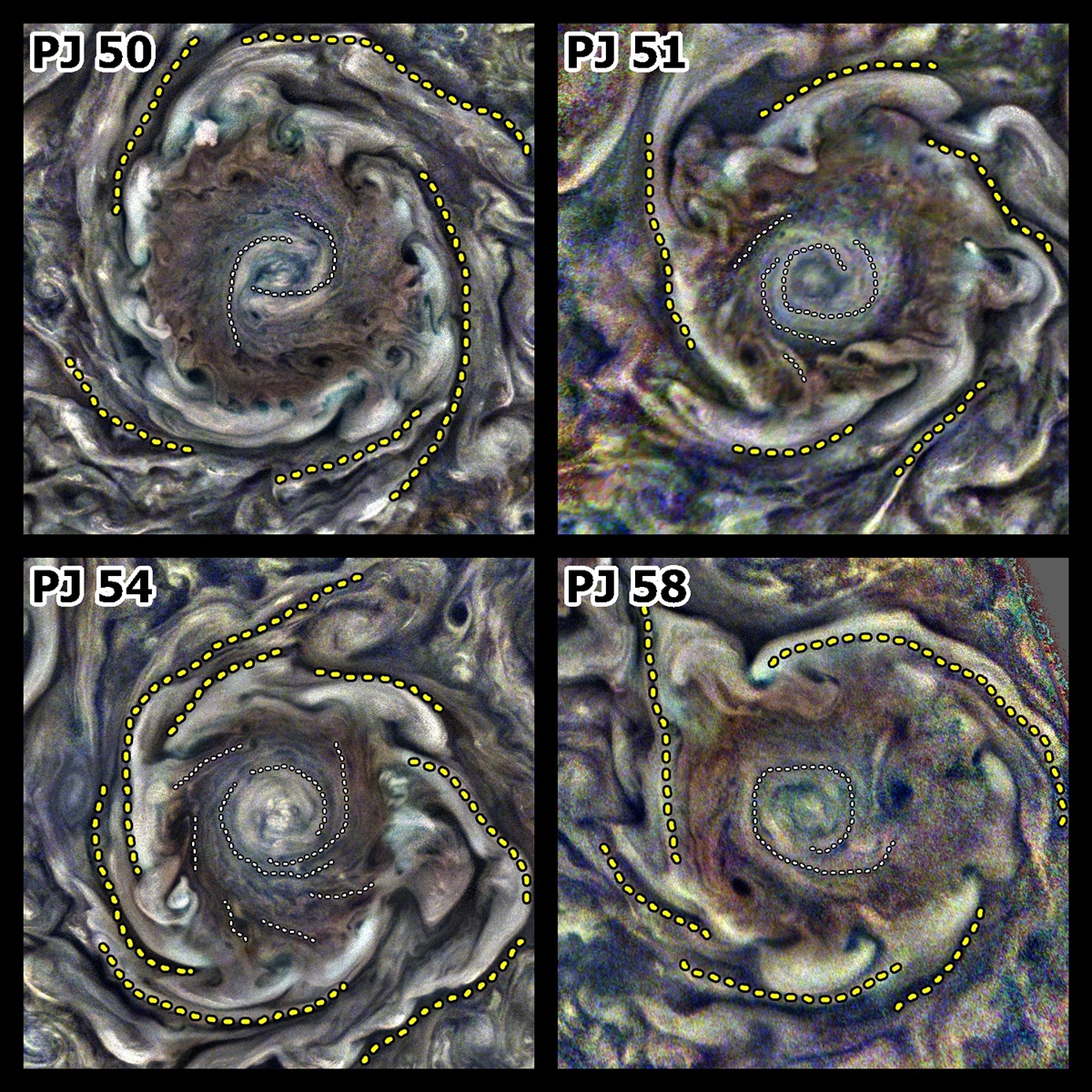
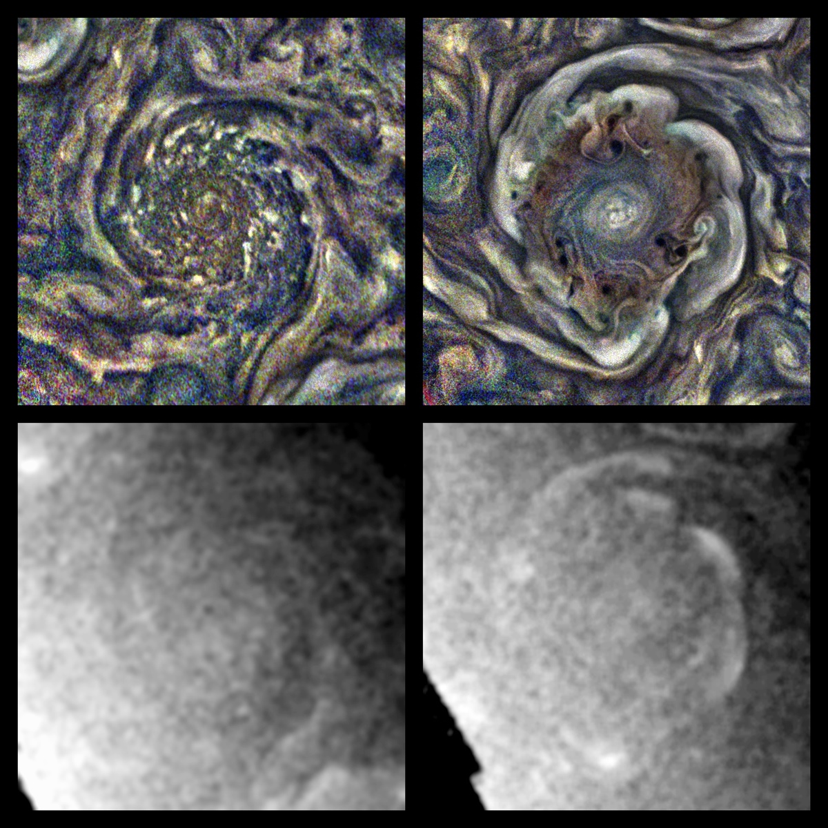
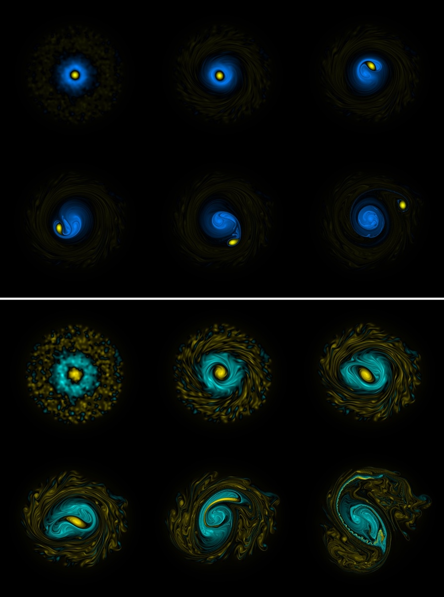
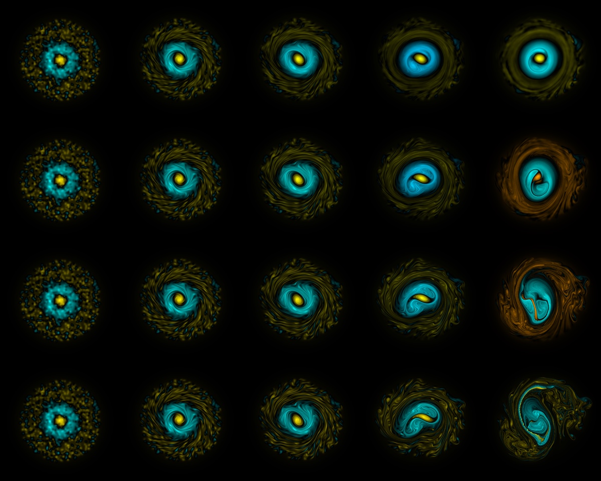
Morphological features and evolution of Jupiter’s Polar Cyclones revealed from JunoCam and JIRAM. , Europlanet Science Congress 2024, Berlin, Germany, 8–13 Sep 2024, EPSC2024-517, https://doi.org/10.5194/epsc2024-517, 2024.

EPSC2024-653
|
On-site presentation
Fran Bagenal, Vincent Dols, Phil Valek, and Hunter Waite

The JADE instrument on Juno has measured cold (<1 eV) heavy ions (sulfur and oxygen) in the equatorial ionosphere of Jupiter as the spacecraft made its closest approach to the planet (~3,500 km above 1 bar level), as reported by Valek et al. (2020) for 17 passes (between perijoves 6 and 23). The source of these heavy ions in Jupiter’s proton-dominated ionosphere remains unclear. The presence of sulfur and oxygen suggests they ultimately came from Io. Inward transport of plasma from the Io torus is slow and the total flux very small. Moreover, adiabatic heating would produce energetic particles reaching the equatorial ionosphere rather than cold populations. An alternative possible source could be neutral atoms that are ejected by the plasma interaction with Io’s atmosphere. We take estimates of the neutral fluxes from models of the Io plasma-atmosphere interaction and explore how the flux of neutrals reaching Jupiter depends on the ejection speed and direction. We then consider typical equatorial atmospheric conditions at Jupiter and evaluate how the incoming neutrals become cold heavy ions mixed into the ionosphere.

How to cite: Bagenal, F., Dols, V., Valek, P., and Waite, H.: Io Source of Heavy Ions in Jupiter’s Equatorial Ionosphere, Europlanet Science Congress 2024, Berlin, Germany, 8–13 Sep 2024, EPSC2024-653, https://doi.org/10.5194/epsc2024-653, 2024.

EPSC2024-778
|
ECP
|
On-site presentation
Giacomo Nodjoumi, Alessandro Mura, Francesca Zambon, Federico Tosi, Melissa Mirino, Mike Ravine, Candy Hansen, Rosaly Lopez, Fran Bagenal, Christina Plainaki, Giuseppe Sindoni, and Scott Bolton

Introduction

Processing JunoCam's raw images of Io to obtain georeferenced images is a critical task in planetary science. Although JunoCam is not a dedicated scientific instrument, it has provided extremely valuable data about Jupiter and its moons, including Io. Producing accurate georeferenced images is especially important now, as the extended mission aims to further study Io and the other Galilean moons.


Io, the innermost of Jupiter's four Galilean moons, is the most geologically active body in the Solar System, with over 400 active volcanoes [1]. This volcanic activity is driven by tidal heating resulting from Io’s orbital resonance with Europa and Ganymede. Observations from JunoCam provide crucial insights into Io's surface composition, volcanic activity, and interior structure.


JunoCam

JunoCam is a CCD sensor equipped with four filters red, green, blue, and methane designed to capture detailed color images of Jupiter and its moons [2]. JunoCam raw images are publicly available in PNG format and composed of multiple framelets of 128 x 1648 pixels, for each RGB filter. The reconstruction of these framelets, the optical distortion corrections, and the segmentation of the target of interests, are fundamental steps to achieve precise georeferenced results. The limb identification process is pivotal for creating accurate map-projected images. Identifying the limb accurately in each framelet allows for precise reconstruction and mapping of the image onto a georeferenced coordinate system.


Workflow Description

In the proposed workflow, raw images are enhanced through multiple Computer Vision (CV) pre-processing steps, to improve contrast and reduce noise, making limb detection more robust. Edge-detection is first applied to the enhanced images, to filter-in the framelets containing the target of interest. Then, segmentation masks are obtained by processing the framelets with the Segment Anything Model (SAM) [3]. Since SAM is class-agnostic, all the obtained masks are filtered by combining the overlapping ones and checking the corresponding DN mean values. This step is crucial for undistorting and map-projecting the framelets accurately.

The segmented framelets are then processed using a pin-hole camera model and SPICE kernels to undistort and map-project them. SPICE kernels provide spacecraft and planetary ephemeris data, which are essential for accurate map projection. The undistorted framelets are then stitched together to reconstruct the final georeferenced image.


Results

The proposed workflow has been tested on several JunoCam images of Io. The results show a good accuracy of georeferenced images, with a reproducible and robust workflow. The limb segmentation step, powered by SAM, is particularly effective in isolating the limb despite the challenging conditions present in raw space images, such as varying lighting and noise levels.


Figure 1. Interface of the interactive plot where users can create and interact with reconstructed uncontrolled mosaics of Junocam images. This tool allows for real-time adjustments and visualization, enhancing the user's ability to fine-tune the reconstruction process.

Figure 2.  Framelet segmentation step: the original raw image (a) and the raw image with segmentation masks superimposed (b). The segmentation masks, shown in red, highlight the detected limb, which is crucial for accurate georeferencing.


Conclusion

The semi-automated robust workflow presented in this paper significantly improves the georeferencing of Junocam images of Io. By leveraging advanced segmentation techniques and adhering to the FAIR principles, this work provides a valuable tool for the planetary science community. Future enhancements could include further automation and integration with other planetary image processing tools.


FAIR Principles

This work adheres to the FAIR principles—Findability, Accessibility, Interoperability, and Reusability—by publishing the workflow code as open-source, ensuring it is easy to use and modify. 

Acknowledgments

This work is supported by the Agenzia Spaziale Italiana (ASI). JIRAM is funded by the ASI–INAF Addendum n. 2016-23-H.3-2023 to grant 2016-23-H.0. Part of this work was performed at the Jet Propulsion Laboratory, California Institute of Technology, under contract with NASA.


References

[1] Zambon, F., Mura, A., Lopes, R. M. C., Rathbun, J., Tosi, F., Sordini, R., et al. (2023). Io hot spot distribution detected by Juno/JIRAM. Geophysical Research Letters, 50, e2022GL100597. https://doi.org/10.1029/2022GL100597

[2] Hansen, C.J., Caplinger, M.A., Ingersoll, A. et al. Junocam: Juno’s Outreach Camera. Space Sci Rev 213, 475–506 (2017). https://doi.org/10.1007/s11214-014-0079-x

[3] Kirillov, A., Mintun, E., Ravi, N., Mao, H., Rolland, C., Gustafson, L., ... & Girshick, R. (2023). Segment anything. In Proceedings of the IEEE/CVF International Conference on Computer Vision (pp. 4015-4026).

How to cite: Nodjoumi, G., Mura, A., Zambon, F., Tosi, F., Mirino, M., Ravine, M., Hansen, C., Lopez, R., Bagenal, F., Plainaki, C., Sindoni, G., and Bolton, S.: 
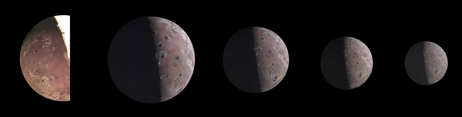
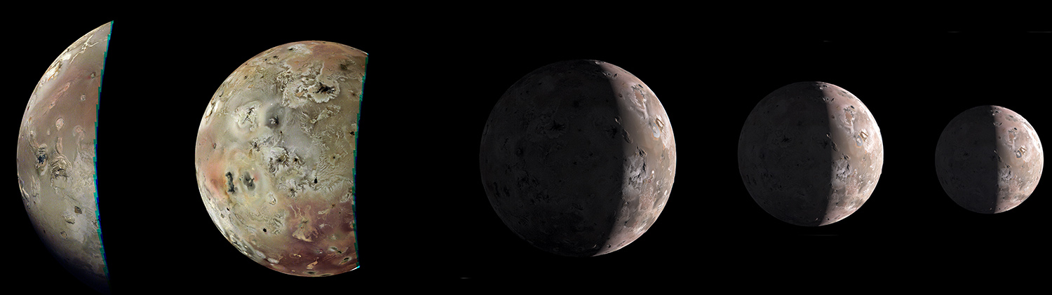
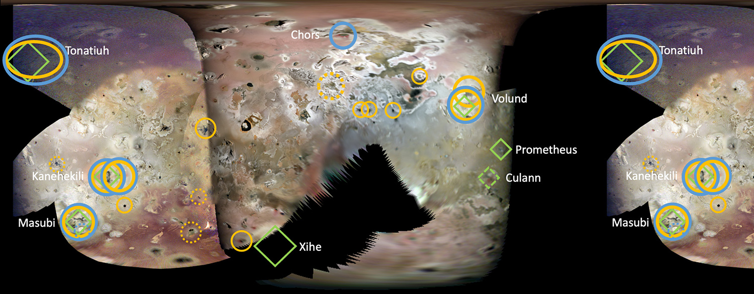
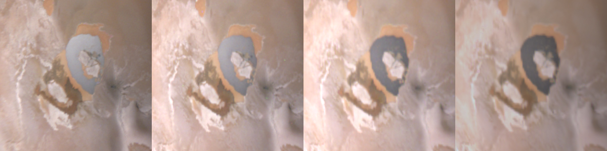
An Enhanced Toolset for JunoCam Images of Io with Interactive Mosaic Visualization and Segmentation-Enhanced Georeferencing, Europlanet Science Congress 2024, Berlin, Germany, 8–13 Sep 2024, EPSC2024-778, https://doi.org/10.5194/epsc2024-778, 2024.

EPSC2024-202
|
On-site presentation
Ricardo Hueso, Marc Delcroix, Agustín Sánchez-Lavega, and Mikel Sánchez

Jupiter is the largest and most massive planet in the Solar System. Because of its active and changing colored atmosphere, it is also the most popular target for amateur astronomers devoted to obtaining planetary images at high spatial resolution. Since 2010 several amateur astronomers have discovered intense flashes of light occurring in Jupiter’s atmosphere. These bright flashes are produced by the collision of objects of 5-35 m in diameter that impact Jupiter’s atmosphere at velocities higher than 60 km/s and release energies of the order of 10^15-10^16 Joules [1-3]. These energies are comparable to the energy released by larger impacts on the Earth, such as the Chelyabinsk impact in 2013. When observed from a distant point these bolides produce enough light to shine briefly for about 1-3 seconds as stars of apparent magnitude 3-7 that become observable with small telescopes. Up to December 2023, 13 such impacts flashes have been observed by amateur astronomers. One of the brightest impacts was discovered by a research team at Kyoto University devoted to search for such impacts [3-4]. This detection included observations in different filters that allowed to constrain a brightness temperature of about 8300 K. Additionally, a smaller impact flash created by an object of 1-4 m was observed by the Juno spacecraft in 2020 [5], providing a spectrum in the UV which results also in high brightness temperatures of 9600 K. These measurements of temperatures are very important, because calibrated light curves of impacts discovered by amateur astronomers require brightness temperatures to disentangle the luminous energy produced in the object, which allows to retrieve estimates of the mass of the objects. In recent years, several observers have been able to observe these impacts simultaneously using a variety of equipment sensitive to different spectral ranges, which agrees with these brightness temperature estimates.

Here we report on the characteristics of 3 impacts detected in 2020-2021 and 4 impacts observed in 2023, two of them observed on consecutive nights on December 28 and 29. Part of the enhanced frequency of these observations corresponds to the global collaboration DeTeCt (http://www.astrosurf.com/planetessaf/doc/project_detect.php), in which more than 250 individual observers monitor the planet frequently with an automatic detection software. This software alerts observers in case of positive detections and also provide statistics of the negative detections obtained. The DeTeCt collaboration has analyzed more than 343,000 video observations of the planet that together represent data equivalent to a full year of continuous observations. From this analysis we update our previous estimate [2] of the current impact rate in the Jupiter system. The new estimate does not differ significantly from our previous estimate of 10-60 bolide impacts in Jupiter for objects in the size range of 10-20 m in diameter. We explore the influence of these objects in the chemistry of the planet’s upper atmosphere and we examine the potential of the JUICE missions to observe fresh craters in Ganymede in its in-depth exploration of this Galilean moon in the 2030s.

References: [1] Hueso, Weslley et al. First Earth-based detection of a superbolide on Jupiter. The Astrophysical Journal Letters, 721(2), L129 (2010).  [2] Hueso, Delcroix et al. Small impacts on the giant planet Jupiter, Astronomy & Astrophysics 617, A68 (2018). [3] Arimatsu et al. Detection of an Extremely Large Impact Flash on Jupiter by High-cadence Multiwavelength Observations The Astrophysical Journal Letters, Volume 933, Issue 1, id.L5, 9 pp. (2022). [4] Arimatsu et al. Cloud reflection modelling for impact flashes on Jupiter. A new constraint on the bulk properties of the impact objects, Astronomy & Astrophysics, 677, id. A165 (2023). [5] Giles et al. Detection of a Bolide in Jupiter's Atmosphere With Juno UVS, Geophysical Research Letters, 48, id. e91797 (2021).

How to cite: Hueso, R., Delcroix, M., Sánchez-Lavega, A., and Sánchez, M.: Bright bolides in Jupiter in 2020-2024: Improving estimations of impact rates on the Jupiter System, Europlanet Science Congress 2024, Berlin, Germany, 8–13 Sep 2024, EPSC2024-202, https://doi.org/10.5194/epsc2024-202, 2024.

EPSC2024-208
|
ECP
|
On-site presentation
Cyril Gapp, Miriam Rengel, Paul Hartogh, Hideo Sagawa, Helmut Feuchtgruber, Emmanuel Lellouch, and Geronimo L Villanueva

Context. On October 31, 2009, the Photodetector Array Camera and Spectrometer (PACS) onboard the Herschel Space Observatory observed far infrared spectra of Jupiter in the wavelength range between 50 and 220µm as part of the program ‘Water and Related Chemistry in the Solar System’. The spectra have an effective spectral resolution between 900 and 3500, depending on wavelength and grating order.

Aims. We investigate the disk-averaged chemical composition of Jupiter's atmosphere as a function of height using these observations.

Methods. We used the Planetary Spectrum Generator (PSG) and the least squares fitting technique to infer the abundances of trace constituents.

Results. The PACS data include numerous spectral lines attributable to ammonia (NH3), methane (CH4), phosphine (PH3), water (H2O) and deuterated hydrogen (HD) in the Jovian atmosphere and probe the chemical composition from p∼275 mbar to p∼900 mbar. From the observations, we infer an ammonia abundance profile that decreases from a mole fraction of (1.7±0.8)x10-4 at p∼900 mbar to (1.7±0.9)x10-8 at p∼275 mbar, following a fractional scale height of about 0.114. For phosphine, we find a mole fraction of (7.2±1.2)x10-7 at pressures higher than (550±100) mbar and a decrease of its abundance at lower pressures following a fractional scale height of (0.09±0.02). Our analysis delivers a methane mole fraction of (1.49±0.09)x10-3. Analyzing the HD R(0) line at 112.1 µm yields a new measurement of Jupiter's D/H ratio, D/H=(1.5±0.6)x10-5. Finally, the PACS data allow us to put the most stringent 3σ upper limits yet on the mole fractions of hydrogen halides in the Jovian troposphere. These new upper limits are <1.1x10⁻¹¹ for hydrogen fluoride (HF), <6.0x10⁻¹¹ for hydrogen chloride (HCl), <2.3x10⁻¹⁰ for hydrogen bromide (HBr) and <1.2x10⁻⁹ for hydrogen iodide (HI) and support the proposed condensation of hydrogen halides into ammonium halide salts in the Jovian troposphere.

How to cite: Gapp, C., Rengel, M., Hartogh, P., Sagawa, H., Feuchtgruber, H., Lellouch, E., and Villanueva, G. L.: Abundances of trace constituents in Jupiter's atmosphere inferred from Herschel/PACS observations, Europlanet Science Congress 2024, Berlin, Germany, 8–13 Sep 2024, EPSC2024-208, https://doi.org/10.5194/epsc2024-208, 2024.

EPSC2024-242
|
On-site presentation
Agustin Sanchez-Lavega, Enrique García-Melendo, Jon Legarreta, Arnau Miró, Manel Soria, and Kevin Ahrens-Velásquez

Jupiter's Great Red Spot (GRS) is probably the best known atmospheric feature and a popular icon among solar system objects. Its huge oval shape, contrasted red color and longevity, have made it an easily visible target for small telescopes. The GRS is the largest and longest-lived known vortex, an anticyclone, of all solar system planets but its lifetime is debated and its formation mechanism remains hidden. G. D. Cassini discovered in 1665 the presence of a dark oval at the GRS latitude, known as the “Permanent Spot” (PS) that was observed repeatedly by him and others, until 1713. After a long period of 118 years without observations of PS, it is in 1831 when the presence at the same latitude of an elongated cavity or hollow in the South Equatorial Belt (SEB) was reported. We show from measurements on historical observations of its size evolution, shrinkage rates, and motions of PS and the GRS and its hollow that the 1831 drawing represents the first record of the proto-GRS. Therefore, PS is unlikely to correspond to the current GRS, and if so, the GRS would be at least 193 years old. Until 1872, the proto-GRS was drawn as a clear oval enclosed by a dark elliptical ring, and it was from that year that was drawn and photographed as a red oval accompanied by the hollow in the SEB (Figure 1) [1].

Recent microwave and gravity field measurements made by Juno spacecraft indicate that the GRS length is likely to be much greater than its depth [2-3]. We have used a Shallow Water (SW) [4] and the Explicit Planetary Isentropic Coordinate (EPIC) [5] models operating for Jupiter upper troposphere conditions to perform numerical simulations on the origin of the GRS. We have explored three different dynamical mechanisms for its genesis: a “super-storm”, the merger of a chain of mid-scale anticyclones, and a long-cell resulting from a shear flow instability. Our numerical simulations rule out the first two scenarios and support that the proto-GRS formed from an instability known as the South Tropical Disturbance [6] that grows between the two opposed Jovian zonal jets north and south of the latitude of the GRS. If so, the early GRS should have had a low tangential velocity so that its rotation velocity has increased over time as it has shrunk.

[1] Sánchez-Lavega, A. et al., 2024. The origin of Jupiter’s Great Red Spot. Geophysical Research Letters (in the press).

[2] Bolton S. J. et al. (2021). Microwave observations reveal the deep extent and structure of Jupiter’s atmospheric vortices. Science 374, 968-972.

[3] Parisi M. et al. (2021). The depth of Jupiter’s Great Red Spot constrained by Juno gravity overflights. Science 374, 964-968.

[4] García-Melendo E., Sánchez-Lavega A. (2017). Shallow water simulations of Saturn’s giant storms at different latitudes. Icarus 286, 241–260.

[5] Dowling T. E., et al. (1998). The explicit planetary isentropic-coordinate (EPIC) atmospheric model. Icarus 132, 221–238.

[6] Rogers J. H. (2008). The accelerating circulation of Jupiter’s Great Red Spot. J. Brit. Astron. Assoc. 118, 14-20.


Fig. 1:  (a) Drawing showing the Permanent Spot (PS) by G. D. Cassini, 19 January 1672. (b) Drawing by S. Swabe in 10 May 1851, showing the proto-GRS as a clear oval with approximate limits marked by a red dashed line. (c) Photograph by A. A. Common on 3 September 1879 showing the GRS as a prominently “dark” oval. (d) Photograph of the GRS and its hollow taken at Lick Observatory on 14 October 1890. (e) SW simulations of the proto-GRS as a circulating long-cell enclosed by a STrD instability. (f) (g) East-West and North-South velocity profiles across the elongated-cell center (marked by the red lines in (e)). All figures show the astronomical view of Jupiter (South up, East left). Adapted from [1].

How to cite: Sanchez-Lavega, A., García-Melendo, E., Legarreta, J., Miró, A., Soria, M., and Ahrens-Velásquez, K.: On the origin of Jupiter’s Great Red Spot, Europlanet Science Congress 2024, Berlin, Germany, 8–13 Sep 2024, EPSC2024-242, https://doi.org/10.5194/epsc2024-242, 2024.

EPSC2024-808
|
On-site presentation
Arrate Antuñano, Pablo Rodriguez-Ovalle, Ricardo Hueso, Thierry Fouchet, Agustín Sánchez-Lavega, Imke de Pater, Tom S. Stallard, Henrik Melin, Glenn S. Orton, Michael Wong, and Leigh N. Fletcher

The NIRCam instrument on JWST obtained high-resolution images of Jupiter at wavelengths between 1.65 µm and 4.05 µm on July 22, 2022 as part of the Early Release Science program 1373 [1]. At these wavelengths and at Jovian high latitudes, polar hazes located in the stratosphere become the dominant features in the images, with little visibility of details in the troposphere, which appear dark due to strong absorptions caused by methane and hydrogen. Ground-based and HST observations of Jupiter’s Polar Regions usually display smooth features in the hazes whose dynamics are difficult to discern due to low contrast and limited spatial resolution. The new JWST views of Jupiter’s polar and sub-polar areas display intriguing stratospheric features, the most remarkable ones being low-albedo, elongated features located at the sub-polar region (near 50°-60° latitude) in 3.35-µm and 3.6-µm images sensing stratospheric hazes and tropospheric clouds.

With the aim of characterising the nature and origin of the dark filaments observed in the sub-polar stratosphere in the JWST images, we examine various sets of images: (i) images taken by the NIRCam instrument on-board the JWST acquired at wavelengths between 1.65 µm and 4.05 µm on July 22, 2022, sensing from the troposphere to the stratospheric hazes; (ii) data taken by NIRSpec instrument on-board the JWST acquired on December 24, 2022, with the F290LP-G395H filter ranging from 3 µm to 5 µm; (iii) images captured by the WFC3 camera on the Hubble Space Telescope acquired at the methane absorption band (889 nm) and in the ultraviolet (275 nm), sensing the tropopause and upper-troposphere respectively, on July 28, 2022; and (iv) JunoCam images taken on August 18, 2022, in the visible channels sensing the cloud-tops. Polar projections of the NIRCam data are shown in Figure 1 and Figure 2, where some of the above-mentioned elongated features are indicated by coloured arrows.

In this talk, we present highlights from the investigation of the polar and sub-polar dynamics and the polar structures observed in the stratosphere of Jupiter. We report the presence of sub-polar dark elongated features in 3.35 µm and 3.6 µm images sensing stratospheric hazes and tropospheric clouds, and compare these features to other potential elongated structures observed in the JunoCam [2] and HST images. We also share an analysis of the sizes, distribution and types of elongated features observed in all the datasets analysed here and present the dynamics of these features by analysing image pairs separated by 10 hours. Finally, by analysing all the results, we propose different candidates that could explain the nature of these features and discuss their potential origin.

Figure 1: Polar projections of Jupiter’s northern hemisphere from images captured on July 22, 2022, by the NIRcam instrument on-board the JWST. Blue arrows indicate some of the dark elongated features and the red arrow indicates a bright-elongated arc.

Figure 2: Same as Figure 1 but for the southern hemisphere. Orange arrows indicate some of the dark elongated features and the green arrow indicates a bright-elongated feature.

References: [1] Hueso, R., Sánchez-Lavega, A., Fouchet, T. et al. An intense narrow equatorial jet in Jupiter’s lower stratosphere observed by JWST. Nat Astron 7, 1454–1462 (2023). [2] Orton, G.S., Rogers, J. et al. Jupiter’s High-Altitude Hazes as Observed by JunoCam. Geophysical Research Abstracts, Vol. 21, EGU2019-3188 (2019).

How to cite: Antuñano, A., Rodriguez-Ovalle, P., Hueso, R., Fouchet, T., Sánchez-Lavega, A., de Pater, I., Stallard, T. S., Melin, H., Orton, G. S., Wong, M., and Fletcher, L. N.: JWST/NIRCAM views of Jupiter's polar regions, Europlanet Science Congress 2024, Berlin, Germany, 8–13 Sep 2024, EPSC2024-808, https://doi.org/10.5194/epsc2024-808, 2024.