TP10 | Planetary Cryospheres: Ices in the Solar System

TP10

Planetary Cryospheres: Ices in the Solar System
Conveners: Oded Aharonson, Silvia Bertoli, Nicole Costa | Co-conveners: Ariel Deutsch, Gianrico Filacchione, Cynthia Sassenroth, Andreas Johnsson, Alice Lucchetti, Costanza Rossi, Shuai Li, Paul Hayne
Orals WED-OB3
| Wed, 10 Sep, 11:00–12:27 (EEST)
 
Room Mercury (Veranda 4)
Orals WED-OB5
| Wed, 10 Sep, 15:00–16:00 (EEST)
 
Room Mercury (Veranda 4)
Posters TUE-POS
| Attendance Tue, 09 Sep, 18:00–19:30 (EEST) | Display Tue, 09 Sep, 08:30–19:30
 
Finlandia Hall foyer, F44–52
Wed, 11:00
Wed, 15:00
Tue, 18:00
Planetary cryospheres encompass environments enriched of volatile ices, in the form of deposits, polar caps, glaciers, and permafrost. Cryospheres are found across the entire Solar System at very different heliocentric distances: on Earth, ice plays a crucial role in landscape evolution as a key hydrological resource and acts as a valuable paleoclimatic indicator.
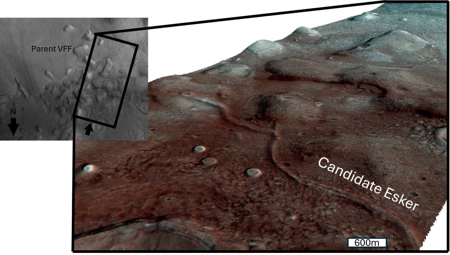
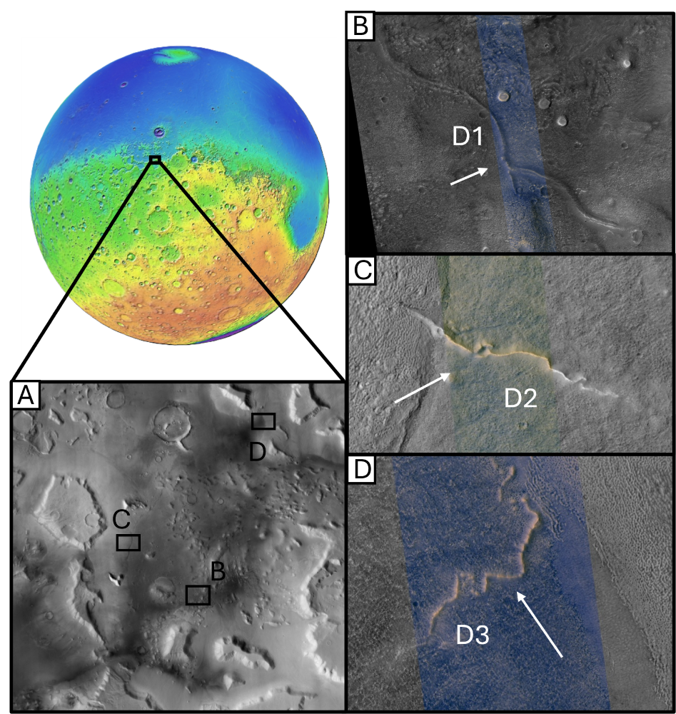
Martian polar caps exhibit analog features to those on Earth, including surface modification and associated landforms, but they also contain CO₂ ice. At mid-latitudes, periglacial landforms—such as polygonal terrains indicate the presence of subsurface ice, while glacier-like features provide evidence of past glacial activity. Moreover, airless bodies such as Mercury and the Moon host icy deposits within the permanently shadowed regions of their polar craters. Further away, beyond the frost line, water ice becomes the dominant compositional endmember. All satellites of Jupiter and Saturn have icy crusts. For some of them (Europa and Enceladus) we have clues for the presence of internal oceans. In addition to water ice, CO₂ and CH₄ also condense into cryosphere at extremely low temperatures. Trans-Neptunian Objects (TNOs), and cometary nuclei are the objects more distant to the Sun and their low temperature and orbital properties allow them to be “time-capsules” because preserve the most primitive material in the Solar System.
Therefore, studying ice on various planetary bodies is crucial for understanding their composition, geological history, climate evolution, and the processes that contributed to the formation of the Solar System.
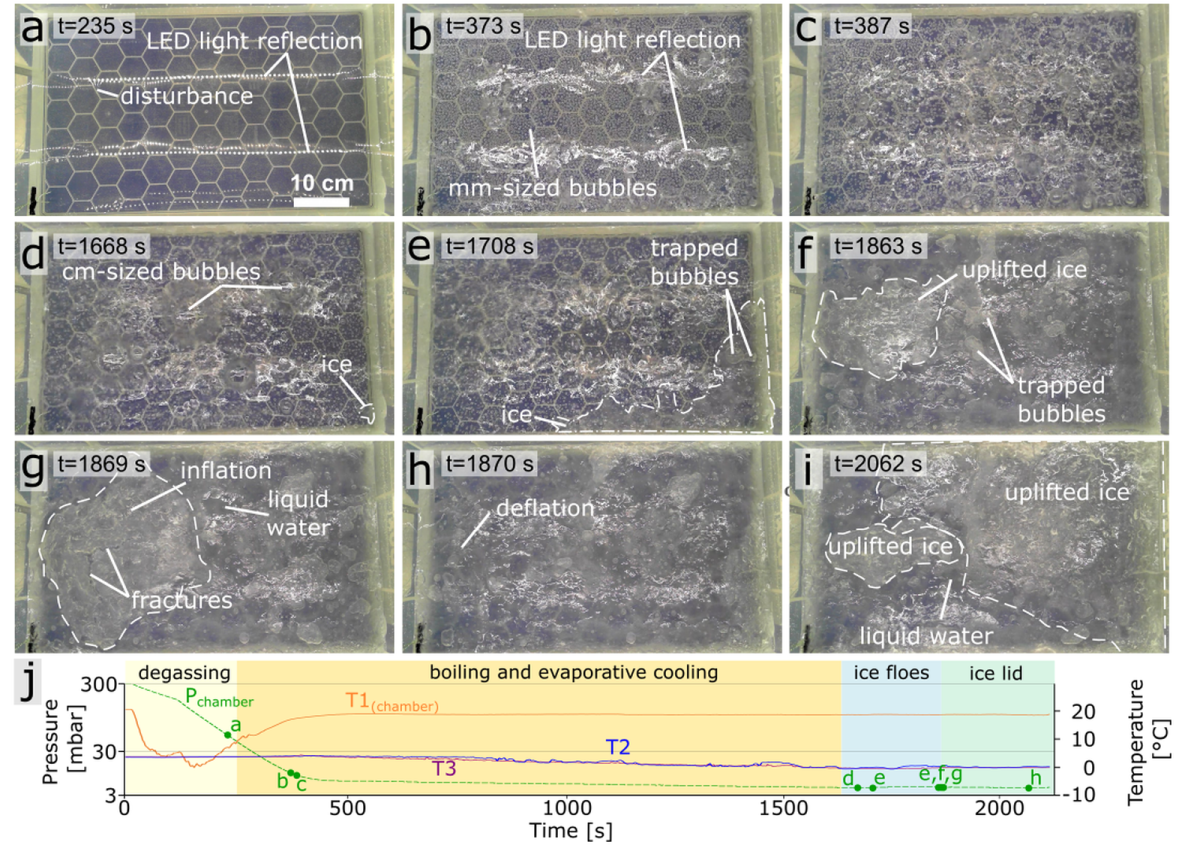
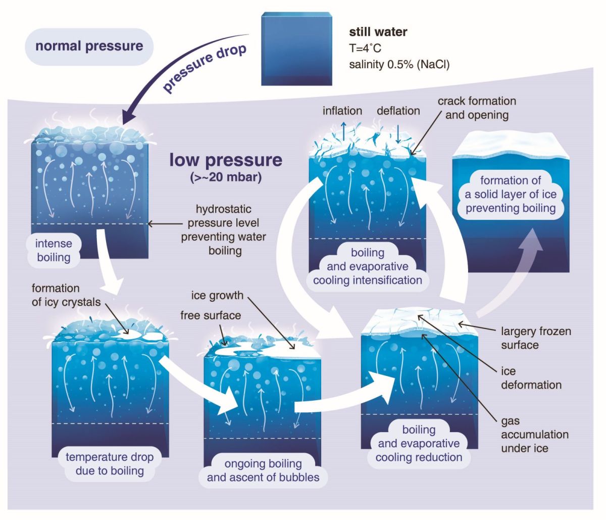
This session welcomes a broad range of contributions, including geological, geophysical and compositional analyses, mapping products, numerical modeling, and laboratory experiments, as well as research incorporating terrestrial analogs.

Session assets

Orals WED-OB3: Wed, 10 Sep, 11:00–12:27 | Room Mercury (Veranda 4)

Chairpersons: Oded Aharonson, Gianrico Filacchione, Alice Lucchetti
Moon
11:00–11:15
|
EPSC-DPS2025-34
|
solicited
|
On-site presentation
Oded Aharonson, Paul Hayne, and Norbert Schorghofer

The lunar polar regions harbor water ice detected directly and indirectly by remotely sensed data. The deposits are concentrated within perennially shadowed regions where water molecules are thermally stable. Owing to the gradual decrease in the lunar spin axis obliquity with time, these regions have grown in extent monotonically since the passage of the Moon through the Cassini State Transition ~4 Ga ago. Combining spectral observations of exposed ice with the theoretical predictions of regions of ice stability constrains the history of accumulation. Using reflected ultraviolet starlight, observations from LAMP exhibit a strong correlation between exposed ice fraction and the age of permanent shadow within which it resides.  This is the first such age relationship that has been identified for the lunar ice, and it indicates ice has accumulated quasi-continuously at least over the last ~1.5 Ga. The exposed ice area ratio of ~5% in the youngest PSRs that have been in shadow over the last ~100 Ma suggests that regolith gardening effectively balances the source and loss rates such that a 1 m layer at least partly equilibrates with the surface over that relatively short timescale.

Finally, we developed a simple model that simulates the sources, sinks, and mixing within the lunar regolith, and show that this model can successfully account for the observations. The model thus provides constraints on the physical parameters and characteristic timescales of the relevant processes.

Figure 1: The LAMP identifications of exposed ice (red, Hayne et al., 2015) superimposed on the PSR ages (blue-white, Schörghofer & Rufu, 2023) with shaded relief in the background.

Figure 2: Cartoon illustrating the simplified regolith gardening and ice accumulation processes our model assumes. At the surface, there is a time-dependent source and a proportional loss term. The domain is assumed to be mixed by a diffusive process.


How to cite: Aharonson, O., Hayne, P., and Schorghofer, N.: The History of Lunar Polar Ice Accumulation, EPSC-DPS Joint Meeting 2025, Helsinki, Finland, 7–13 Sep 2025, EPSC-DPS2025-34, https://doi.org/10.5194/epsc-dps2025-34, 2025.

11:15–11:27
|
EPSC-DPS2025-660
|
ECP
|
On-site presentation
Eric Volkhardt, Johanna Bürger, and Jürgen Blum

Evidence for the presence of water ice at the lunar poles has been gathered using various methods, including radar (e.g., Nozette et al., 2001; Campbell et al., 2006), far-ultraviolet (e.g., Gladstone et al., 2012; Hayne et al., 2015) and laser (Zuber et al., 2012; Lucey et al., 2014) reflectance measurements, neutron spectroscopy (e.g., Feldman et al., 2001), as well as the LCROSS impact experiment (Colaprete et al., 2010). Another more indirect approach involves identifying potential water ice stability regions by combining three-dimensional illumination models of the lunar terrain with thermal models that predict surface and subsurface temperatures. Several studies have utilized this method (e.g., Paige et al., 2010b; King et al., 2020; Formisano et al., 2024), with the main differences between models relating to the level of detail in modeling the illumination source, radiative transfer, and subsurface heat transport.

In this work, we combine the one-dimensional microphysical model for the lunar regolith layer developed by Bürger et al. (2024), which more directly simulates regolith properties, such as grain size and packing-density stratification, with a three-dimensional radiative flux model including topography. This model applies the ray-tracing technique to describe the amount of incoming and reflected solar flux as well as the reflected thermal emission received for every surface element of the investigated area. The radiative transfer model is based on Potter et al. (2023), but the equations are modified to allow for an incidence angle-dependent albedo. Bolometric temperatures measured by the LRO/Diviner lunar radiometer (Paige et al., 2010a) serve as a reference for the modeled surface temperatures and it is demonstrated that the key thermal trends are accurately reproduced.

During the modeling process, we identified several key factors for a correct simulation. First, at high latitudes where the Sun remains near the horizon, it is crucial to model the Sun as a disk rather than a point source to avoid inaccuracies in temperature simulations during sunrise and sunset. Second, to more accurately capture the illumination conditions for the thermal model, the area in which ray-tracing is applied should extend beyond the region where temperatures are modeled. When examining the effect of an incidence angle-dependent albedo, we found that the steep increase in albedo at high incidence angles—required by previous thermal models of global regolith properties (e.g., Hayne et al., 2017; Feng et al., 2020; Bürger et al., 2024)—does not agree with the observed Diviner bolometric temperatures near the poles. Instead, a much weaker dependency, as adopted by King et al. (2020), results in a better fit. Finally, when assessing subsurface water-ice stability, it is crucial to account for the diffusion barrier that reduces sublimation loss rates, as described by Schorghofer & Williams (2020), yielding shallower stability depths. 

Two areas of interest are modeled in detail: First, the Shackleton crater, which is located almost exactly at the lunar south pole and therefore experiences a unique illumination pattern with the crater rim being continuously illuminated and the inner part being in permanent shadow. The second area investigated is the landing site of NASA’s CLPS CP22 mission located on the Leibnitz Plateau. Onboard this mission will be ESA’s PROSPECT instrument, which consists of a drill and a chemical laboratory designed to analyze volatiles (Trautner et al., 2024). Accurate predictions of water ice stability depths are crucial for this mission. Figure 1 illustrates the simulated surface temperatures at three different local times at the CP22 landing site.

At the conference we will present surface temperature and water-ice stability maps of these two regions and discuss the key lessons learned during the modeling process.

Figure 1: Simulated surface temperatures at the CP22 landing site on the Leibnitz Plateau. Illustrated are the surface temperatures at three different local times (left: ~4:30 h, center: ~10:30 h, right: ~16:30 h) with the direction of the Sun being indicated as well.

References

Bürger, J. et al. (2024), JGR Planets, 129, E008152. Campbell, D. B. et al. (2006), Nature, 443, 835-837. Colaprete, A. et al. (2010), Science, 330.6003, 463-468. Feldman, W. C. et al. (2001), JGR Planets, 106, 23231 – 23251. Feng, J. et al. (2020), JGR Planets, 125(1). Formisano et al. (2024), PSS, 251, 105969. Gladstone, G. R. et al. (2012), JGR Planets, 117, E00H04. Hayne, P. O. et al. (2015), Icarus, 255, 58-69. Hayne, P. O. et al. (2017). JGR Planets 122.12, 2371–2400. King, O. et al. (2020). P&SS, 182, 104790. Lucey, P. G. et al. (2014), JGR Planets, 119, 1665-1679. Nozette, S. et al. (2001), JGR, 106, 23253-23266. Paige, D. A. et al. (2010a), Space Sci. Rev., 150(1–4), 125–160. Paige, D. A. et al. (2010b). Science, 330.6003, 479–482. Potter, S. F. et al. (2023). J. Comput. Phys., X 17, 100130. Trautner, R. et al. (2024), Front. Space Technol., 5, 1331828. Schorghofer, N. & Williams, J.-P. (2020), Planet. Sci. J., 1, 54. Zuber, M. T. et al. (2012), Nature, 486, 378-381.

How to cite: Volkhardt, E., Bürger, J., and Blum, J.: Predicting water ice stability depths at the lunar poles by combining a microphysical thermal model with a 3D radiative flux model, EPSC-DPS Joint Meeting 2025, Helsinki, Finland, 7–13 Sep 2025, EPSC-DPS2025-660, https://doi.org/10.5194/epsc-dps2025-660, 2025.

11:27–11:39
|
EPSC-DPS2025-1411
|
On-site presentation
Michelangelo Formisano, Andrea Raponi, Matteo Teodori, Silvia Bertoli, Mauro Ciarniello, Simone De Angelis, Maria Cristina De Sanctis, Gianrico Filacchione, Alessandro Frigeri, Luca Maggioni, and Gianfranco Magni

Introduction

Using the Moon as a case study, we investigate how small-scale surface roughness influences the thermal behavior of airless planetary bodies through self-heating effects. Indirect solar radiation, reflected and scattered by rough terrain, can warm otherwise shaded regions, particularly in highly irregular surfaces or concave topographies such as craters. This process can raise local temperatures by several kelvin, potentially affecting the stability of surface ices in micro cold traps. Our numerical model (e.g. [1]) accounts for both vertical and lateral heat exchange and simulates various rough surface configurations representative of lunar polar regions. We provide temperature maps, quantify self-heating contributions, and estimate the persistence of volatiles. These results may inform Lagrangian models (e.g., SPH codes) aimed at simulating volatile transport and exosphere formation [2].

Numerical Modeling

Before applying our 3D FEM model (e.g., [1]) using COMSOL Multiphysics, we generate synthetic rough surfaces with average slopes consistent with lunar surface roughness estimates found in the literature [3]. We produce eight terrains with mean slopes ranging from 2.5° (nearly flat terrain) to 40° (very rough surface). The method used to synthesize these surfaces is based on a sum of trigonometric functions, similar to a Fourier series expansion, where each term represents a specific spatial frequency of oscillation. In Fig.1, we show two of the synthetic surfaces: the left panels display the surface with a mean slope of 20°, while the right panels show the surface with a mean slope of 40°. The numerical code used to compute surface temperature accounts for both direct and indirect solar radiation, the latter known as self-heating. For these simulations, we arbitrarily choose a latitude of 80°, a heliocentric distance of 1 AU, and a global thermal inertia of 100 TIU.

Preliminary Results And Conclusions

For each of the analyzed surfaces, we produced maps of surface temperature, direct solar illumination, and indirect illumination (due to self-heating), as shown in Fig.2. The threshold temperature adopted to assess the stability of water ice is 110 K, corresponding to a sublimation rate of approximately 100 kg/(Gyr m2 ), and thus to a survival timescale consistent with the age of the Solar System. Our preliminary results suggest the existence of a threshold mean slope-around 20°-that separates two distinct regimes. At low slopes (0-20°), shadowing dominates over self-heating, enabling the formation of cold traps [4]. In contrast, at higher slopes (>20°), self-heating becomes the dominant effect, hindering the preservation of water ice. The set of scenarios developed in this work will be further refined to provide a useful dataset for various planetary contexts.

Figure 1: Examples of the analyzed surfaces: the left panels present the case with a mean slope of 20°, while the right panels show the case with a mean slope of 40°.

Figure 2: Case 1: (A) Incoming flux from direct solar illumination; (B) Incoming flux from indirect illumination due to self-heating of the terrain; (C) Surface temperature map: the blue color scale is limited at 110 K-the stability threshold for cold traps-to emphasize areas where cold traps may be present. The selected time corresponds to local noon.

References

[1] Formisano M., et al., 2024, Planetary and Space Science, 251, 105969
[2] Teodori M., et al., 2025, Icarus (under review).
[3] Helfestein P. & Shepard M. K., 1999, Icarus, 141, 107
[4] Hayne P. et al., 2017, JGR Planets, 122, 2371.

How to cite: Formisano, M., Raponi, A., Teodori, M., Bertoli, S., Ciarniello, M., De Angelis, S., De Sanctis, M. C., Filacchione, G., Frigeri, A., Maggioni, L., and Magni, G.: Thermal Role of Self-Heating and Surface Roughness in Micro Cold Trap Stability at the Lunar Poles, EPSC-DPS Joint Meeting 2025, Helsinki, Finland, 7–13 Sep 2025, EPSC-DPS2025-1411, https://doi.org/10.5194/epsc-dps2025-1411, 2025.

11:39–11:51
|
EPSC-DPS2025-2024
|
On-site presentation
Lior Rubanenko, Jean-Pierre Williams, and Matthew Siegler

Introduction

Lunar permanent shadowed regions (PSRs) may cold-trap and preserve volatile species for geologic time periods [1, 2]. In the past decades, surface and near-subsurface ice at concentrations of  was mapped on the Moon from orbit, as well as directly observed in the plume excavated by the LCROSS impact [3–7]. The absence of radar-bright features in PSRs further suggest that if any substantial ice persists on the Moon, then it is likely intimately mixed with the regolith [8].

Here, we hypothesize that if sufficiently concentrated subsurface ice persists within lunar cold traps, then it should increase the thermal conductivity of the subsurface – and decrease the amplitude of the diurnal thermal wave observed by Diviner.

Methods

Early observations of the Moon have found thermal emissions from the surface deviate significantly from Lambert scattering, and that this deviation can be well-explained by subpixel surface slopes casting shadows and emitting heat directionally. Under oblique illumination conditions, such as at the lunar poles, this aniostropic emission could increase the temperatures of PSRs through beaming [9, 10].

Previous thermophysical simulations of the Moon have neglected anisotropic scattering, and assumed the lunar surface behaves as a Lambert radiator [2]. This assumption resulted in a systematic underprediction of diurnal and annual maximum PSR temperatures compared to those recorded by Diviner (Figure 1). To address the disagreement found by those studies, we develop a thermophysical model which includes anisotropic (non-Lambert) surface emissions, and use it to re-calculate the surface heat balance in PSRs.

Our new model accepts generalized topography as input, and simulates insolation, scattering and thermal emissions between neighboring slopes using ray casting, as well as subsurface conduction [11]. However, instead of assuming each model facet is isothermal and thus radiates heat isotopically, we assume it is composed of subpixel surface slopes with some temperature distribution . To compute , we adapt a well-established statistical approach [9, 12] to any illumination and observation angles  and .  The model assumes subpixel surface slopes, whose directional components are , are distributed Gaussian, with zero mean and root mean square . This allows computing the radiance emitted by each surface element  as, where  is the Gaussian probability density function,  is the angle between the normal to each facet and the emission direction,  is the Stefan Boltzmann constant, and where both integrations are performed only over the part of the surface visible to the observer. Our anisotropic radiance model was tested and agrees with directional emissions measured by Diviner.

Results

We simulate the temperatures of 25 polar craters (15 southern, 10 northern) at peak southern polar summer, initially assuming radiative equilibrium, and find our new model effectively corrects the previously observed systematic underprediction for non-cold-traps (maximum temperatures > 100 K). However, for cold traps (maximum temperatures < 100 K), we find model-simulated maximum temperatures are warmer than Diviner-measured maximum temperatures, suggesting their thermal conductivities are elevated compared to non-cold-trapping surfaces (Figure 1). Using a 1-D thermal diffusion model with the simulated scattered flux as input, we fit the diurnal amplitude of the thermal wave in each PSR location to estimate its thermal conductivity and potential ice content. We find that the elevated model maximum temperatures are best explained by a volumetric mixture of ice and regolith, with up to 10%wt.

Figure 1.

Conclusion

Here, we apply a new thermal model which accounts for anisotropic emissions from the lunar surface, to resolve previous discrepancies [2] between model-simulated and Diviner-measured temperatures of permanently shadowed regions. We find that when assuming radiative equilibrium, model simulated maximum temperatures of cold-trapping PSRs (maximum measured temperatures < 100 K) are higher than measured temperatures, and hypothesize this disagreement is caused by the presence of ground ice, which increases the thermal conductivity of the surface and decreases the amplitude of the diurnal thermal wave. Using a 1-D thermal diffusion model, we find this decreased thermal wave amplitude is best explained by the presence of up to 10%wt ice, in agreement with previous observations (Figure 2).

Compared to exposed ice, buried ice is significantly more resistant to heating and other destructive mechanisms such as photolysis and impact gardening. As a result, our newly mapped deposits likely preserve water and other volatiles for much longer time periods – and thus offer insight into the historical composition of these substances through time.

Figure 2.

References:

[1]       Watson et al. (1961), J. Geophys. Res. 66
[2]       Paige et al. (2010), science 330
[3]       Hayne et al. (2015), Icarus 255
[4]       Fisher et al. (2017), Icarus 292
[5]       Li et al. (2018), Proc. Natl. Acad. Sci. 115
[6]       Mitrofanov et al. (2010), Science 330
[7]       Colaprete et al. (2010), Science 330
[8]       Campbell et al. (2006), Nature 443
[9]       Smith (1967), J. Geophys. Res. 72
[10]     Rozitis and Green (2011), Mon. Not. R. Astron. Soc. 415
[11]     Rubanenko and Aharonson (2017), Icarus 296
[12]     Bass and Fuks (2013), 93

How to cite: Rubanenko, L., Williams, J.-P., and Siegler, M.: Thermal Spectroscopy Reveals Pervasive Deposits of Ground Ice in the Southern Polar Region of the Moon, EPSC-DPS Joint Meeting 2025, Helsinki, Finland, 7–13 Sep 2025, EPSC-DPS2025-2024, https://doi.org/10.5194/epsc-dps2025-2024, 2025.

Icy bodies
11:51–12:03
|
EPSC-DPS2025-1647
|
ECP
|
On-site presentation
Jessica Hogan, Mark Fox-Powell, Rachael Hamp, Victoria Pearson, and Manish Patel

Background

The plumes of Saturn’s moon Enceladus emit water vapour and ice grains from cracks in the ice shell, fed by vents that transport subsurface ocean material upwards to the surface [1]. These ice grains have varied compositions, but the salt-rich population (“Type III”) are interpreted to originate as dispersed ocean spray droplets representative of the subsurface ocean composition [2]. It is assumed that Type III grains can therefore be used as a tool to interpret the chemistry and habitability of the otherwise inaccessible subsurface.  However, from the subsurface ocean to space, ocean fluid ascends through an extreme temperature and pressure gradient, and it is not yet understood how this influences the composition of ejected ice grains. There have also been observations of size-dependent, compositional stratification in the plumes, wherein larger grains fall back to the surface and smaller grains are ejected further from the plume source [3]. This implies that different droplet sizes experience a different cooling rate when exposed to the same plume temperatures. Since cooling rate influences composition [4], there is a likely compositional difference between grain sizes that deposit on the surface and those that escape. Therefore, high-altitude plume sampling by spacecraft and observations of surface fallout may provide different compositional information about the subsurface ocean material.

The focus of this work is to understand the relationship between droplet size and composition, and specifically how salts such as sodium chloride, carbonates, and phosphates, which are believed to be present in the subsurface ocean [2, 5], behave during freezing. By quantifying the solid phase composition of frozen droplets of simulated Enceladus ocean composition, we can establish whether compositional differences exist across a range of grain sizes.


Methods

We designed a fluid simulant representative of Enceladus’ ocean derived from salt constituents confirmed by Cassini measurements of the plume [5, 6], and with a pH of 10 (a midpoint encompassing estimates [7, 8]). Experimental simulations of ice grain formation allowed us to assess how grain size affected the composition and spatial distribution of salts within a droplet. Through quenching aliquots of the fluid across a wide range of droplet volumes (≤ 1× 10 ─ 4 µL, 0.5 µL, 5 µL)  in liquid nitrogen (Figure 1), fluids undergo flash-freezing (>10 K s-1) designed to simulate freezing rates relevant to the plume-forming regions on Enceladus. Utilising scanning electron microscopy-energy dispersive spectroscopy (SEM-EDS) and X-ray diffraction (XRD), we studied the elemental composition, mineralogy and physical partitioning of solid phases within ice grains and how this varies across grains of different volumes. Introducing a range of droplet sizes into the same thermal environment provides variation in bulk cooling rate [10], applicable to grains of different size fractions in the Enceladus plumes.

Figure 1 – Optical microscopy image of flash-frozen ice grains mounted onto quartz slide (10-100 µm size).


Results

Preliminary SEM-EDS analysis of the 0.5 and 5 µL grains detected the formation of sodium chloride, sodium carbonate and sodium phosphate salts. The micro-scale arrangement of these salts differed - sodium carbonate/bicarbonate manifested as relatively flat sheets of rounded, globular nodules of sub-micron size, whereas sodium chloride salt fibres are isolated in striated, parallel ridges across both droplet sizes (Figure 2). At the 100 µm scale, all salts appear embedded together in a matrix across the droplet sizes, but heterogeneities in their distribution become visible under higher magnification. Textural differences between droplet sizes were expressed, with vesicle-like pore spaces and compositional heterogeneity between salts visible at the 10 µm scale in the 5 µL grains. By contrast, the 0.5 µL grains consist of a finer microstructure, with morphological differences from the partitioning of various salts displayed at the 5 µm scale. Compositional heterogeneities are expressed at different scales dependent on grain size, and whether such differences are visible at mineralogical level will be studied in follow-up analyses.

Figure 2 - SEM image capturing the microstructure of NaCl features within a flash-frozen 0.5 µL ice grain.


Next steps

The focus of ongoing analysis will be the solid phase composition of the smallest grain size (≤ 1× 10 ─ 4 µL) and quantifying the phase abundance in all ice grains using cryo-Raman and XRD. Additionally, future work will assess how composition and grain microstructure is affected by the presence and absence of organics that preferentially form with specific solid phases and may be present in plume material [11]. These findings enable us to predict potential compositional differences between grain sizes, and to understand how organics are incorporated, between the largest grains that fall back to the surface and the smaller grains that achieve escape velocity.


References

[1] Porco, C. C. et al. (2006). Science. 311(5766), 1393-1401; [2] Postberg, F. et al. (2009). Nature 459, 1-4; [3] Postberg, F. et al. (2011). Nature 474, 620-622; [4] Fox‐Powell, M. G. (2021). J. Geophys. Res. Planets 126; [5] Postberg, F. et al. (2023). Nature, 618(7965), 489-493; [6] Postberg, F. et al. (2009). Nature, 459(7250), 1098-1101; [7] Zolotov, M. Y. (2012). Icarus 220, 713–729; [8] Glein, C. R. et al. (2018). The Geochemistry of Enceladus: Composition and Controls. Enceladus and the Icy Moons of Saturn, 39; [9] Postberg, F. et al. (2018). Nature 558, 564; [10] Adda-Bedia, M. et al. (2016). Langmuir 32.17, 4179-4188; [11] Khawaja, N. et al. (2019). MNRAS 489.4, 5231-5243.

How to cite: Hogan, J., Fox-Powell, M., Hamp, R., Pearson, V., and Patel, M.: Size-Dependent Composition of Ice Grains Relevant to Salt-Rich Particles in the Plumes of Enceladus, EPSC-DPS Joint Meeting 2025, Helsinki, Finland, 7–13 Sep 2025, EPSC-DPS2025-1647, https://doi.org/10.5194/epsc-dps2025-1647, 2025.

12:03–12:15
|
EPSC-DPS2025-853
|
ECP
|
On-site presentation
Lucas Lange and Sylvain Piqueux

NASA's Europa Clipper mission will characterize the current and recent surface activity of the icy-moon Europa through a wide range of remote sensing observations. In particular, the Europa Thermal Emission Imaging System (E-THEMIS) will measure global, regional and local surface temperatures at three thermal infrared wavelengths, under various conditions of local time and emission angles [1]. These measurements will not only enable the detection and characterization of thermal anomalies on the surface, but also provide insight into the thermophysical properties of the regolith, such as particle size, block abundance, and subsurface layering.

Indeed, in the absence of endogenic heat-sources, Europa's surface temperatures are controlled by the albedo and thermal inertia of the surface. To date, these properties have been derived for Europa by comparing the surface temperature modeled by 1D thermal model with measurements from either ground-based observations [e.g., 2,3], Voyager 1 flyby [4] or by the PPR instrument onboard the Galileo spacecraft at the end of the 20th century [5,6].

The thermophysical properties of granular porous ice, as expected on Europa, differ fundamentally from silica-based trends usually considered by thermal models applied to rocky bodies [7]. Specifically, the bulk thermal conductivity of ice can vary by several orders of magnitude [7], depending on the microphysical properties of ice (crystallinity, ice crystal radius, porosity, contacts between ice crystals) and temperature (Fig. 4). Importantly, radiative conductivity within water ice fines is always neglected in models used to date [3,8-11], while it is a major contributor in the conductivity of particulate water ice, even at the low Europa temperatures [7]. Furthermore, [7] demonstrated that the contact conductivity for small-size ice crystals was controlled by the nature of contacts between ice grains. As a consequence, while the thermal conductivity for silica-based material decreases with decreasing grain size, [7] demonstrated that porous ice made of micrometer size ice crystals follows an opposite trend, and yields high thermal inertia (Fig. 4a), potentially inducing high nighttime temperatures compared to those expected with coarser material (e.g., +20 K in the case illustrated in Fig. 4b). Because the surface of Europa is thought to expose both crystalline and amorphous ice, with very small ice crystals [12,13], it is important to understand the differential thermal regimes that could results from various icy materials configurations, especially to avoid the erroneous identification of thermal anomalies as endogenic hotspots.

To account for this new knowledge, we are improving the KRC -K for k, symbol of thermal conductivity, R for rho (density), and C for Cp (specific heat) -  thermal model [8], which has been extensively used for planetary surfaces thermophysical studies, and which will be used for the interpretation of future E-THEMIS data. We have incorporated state-of-the art thermal inertia dependencies to ice properties described in [7], and we are currently implementing the emissivity dependency to ice temperature [e.g.,14], the penetration of solar radiation within the icy surface to simulate solid-state greenhouse effect [e.g., 15], and subsurface layering. At the conference, we will present model predictions for surface temperature signatures resulting from these physical processes, and compare them with PPR observations. This comparison enables us to place constraints on Europa's near-surface properties, including porosity, grain size, and potential layering. Ultimately, this work aims to refine the interpretation of upcoming E-THEMIS thermal observations and help distinguish between thermophysical and endogenic origins of thermal anomalies on Europa.


Figure 1: Effects of (a) the ice properties on thermal inertia [7] compared to silicate trends and (b) on Europa’s temperatures (computed with KRC). A surface composed of fine small crystalline grains can exhibit an unexpected high  thermal inertia, inducing a +20 K nighttime warming compared to the surrounding surfaces, and be thus  misinterpreted as a hot-spot.


References: [1] Christensen et al. (2024), The Europa Thermal Emission Imaging System (E-THEMIS) Investigation for the Europa Clipper Mission, Space Science Reviews; [2] Hansen (1973),  Ten-micron eclipse observations of Io, Europa, and Ganymede. Icarus; [3] Trumbo et al. (2018), ALMA thermal observations of Europa. Astronomical Journal; [4] Spencer (1987), The surfaces of Europa, Ganymede, and Callisto: an investigation using Voyager IRIS thermal infrared spectra (Jupiter). PhD thesis at the University of Arizona; [5] Spencer et al. (1999), Temperatures on Europa from Galileo photopolarimeter-radiometer: nighttime thermal anomalies, Science; [6] Rathbun et al. (2010), Galileo PPR observations of Europa: hotspot detection limits and surface thermal properties, Icarus; [7] Ferrari & Lucas (2016), Low thermal inertias of icy planetary surfaces, Astronomy and Astrophysics; [8] Kieffer (2013), Thermal model for analysis of Mars infrared mapping, JGR: Planets; [9] Spencer et al. (1989). Systematic biases in radiometric diameter determinations, Icarus; [10] Hayne et al. (2017), Global regolith thermophysical properties of the Moon from the Diviner Lunar Radiometer Experiment, JGR: Planets; [11] Thelen et al. (2024), Subsurface Thermophysical Properties of Europa’s Leading and Trailing Hemispheres as Revealed by ALMA, The Planetary Science Journal; [12] Berdis et al. (2020), Europa’s surface water ice crystallinity: Discrepancy between observations and thermophysical and particle flux modeling, Icarus; [13] Hansen, & McCord (2004), Amorphous and crystalline ice on the Galilean satellites: A balance between thermal and radiolytic processes, JGR: Planets; [14] Ferrari (2024), Infrared emissivity of icy surfaces. Sensitivity to regolith properties and water-ice contaminants, Astronomy and Astrophysics; [15] Brown & Matson (1987), Thermal effects of insolation propagation into the regoliths of airless bodies, Icarus.

Acknowledgement: This work was performed at the Jet Propulsion Laboratory, California Institute of Technology, under a contract with NASA (80NM0018D0004). LL’s research was supported by an appointment to the NASA Postdoctoral Program at the Jet Propulsion Laboratory, administered by Oak Ridge Associated Universities under contract with NASA.

How to cite: Lange, L. and Piqueux, S.: Near-Surface Properties of Europa Constrained by the Galileo PPR Measurements , EPSC-DPS Joint Meeting 2025, Helsinki, Finland, 7–13 Sep 2025, EPSC-DPS2025-853, https://doi.org/10.5194/epsc-dps2025-853, 2025.

Mars
12:15–12:27
|
EPSC-DPS2025-1794
|
On-site presentation
Ernst Hauber, Harald Hiesinger, Nico Schmedemann, Andreas Johnsson, Michael Zanetti, Cynthia Sassenroth, Tilman Bucher, Matthias Geßner, Michael Angelopoulos, Adam Johantges, Bernard Hallet, Julia Boike, Guido Grosse, Ivar Berthling, and Jaakko Putkonen

Recent and present non-polar ice deposits (e.g., [1-6]) are important records of the changing dynamics of the Martian climate and constitute an important resource for possible future in-situ resource utilization (ISRU) [7]. Recently the mapping of such ice deposits has gained significant momentum, as several projects (e.g., SWIM; [8-9]) addressed the distribution of such deposits, and dedicated space missions have been suggested to study such deposits and their links to the climate history (e.g., COMPASS [10]; I-MIM/International Mars Ice Mapper Mission [11]; IceBreaker [12]; ice drilling plans of ESA and NASA, such as the ice-drilling Mars Life Explorer lander). Many of these ice deposits are associated with landforms that resemble glacial and periglacial surface features on Earth [13]. Moreover, a number of landforms on Mars have been hypothesized to have formed by the action of liquid water in the last few millions of years, and possibly even until today (e.g., [14]). Such landforms include, but are not restricted to, gullies and associated depositional fans, patterned ground, and flow lobes on slopes, which have been interpreted as evidence for debris flows, freeze-thaw cycles, and solifluction, respectively (e.g., [15-17]). However, under current conditions (low T, thin atmosphere), liquid water is not stable at the surface of Mars unless special conditions are met (e.g., [18-19]), although contemporary subsurface liquid water is debated [20]. Hence, a reconstruction of the planet’s recent climate history involving liquid water is challenging (e.g., [21,22]). Furthermore, as morphologic interpretations are typically not unambiguous (the concept of equifinality, e.g., [23]), most if not all of these landforms may also have formed by alternative “dry” processes (see, e.g., the study of polygonal textures in Gale crater by ref [24]).

Fieldwork on terrestrial analogues is considered essential to understand planetary landforms and their evolution, as the Earth is still our “reference” to understand geologic processes [25]. The knowledge gained by fieldwork helps to establish multiple working hypotheses and test them (e.g., for the case of polygonal ground see ref [26]).

The remote Arctic archipelago of Svalbard constitutes  a unique terrestrial analog environment for comparison to latitude-dependent cold climate landforms on Mars. Svalbard contains abundant periglacial features in close proximity, allowing for an integrated landscape analysis approach to understand the evolution of cold climate landforms on Earth and Mars.

The main questions driving our fieldwork on Svalbard are:

  • Does the formation of cold-climate landforms on Mars require freeze-thaw processes and the melting of snow/ice (i.e., was there liquid water involved in their formation)?
  • What are the rates of cold-climate processes on Mars (i.e. what are the possible time scales of their formation)?
  • How do analogous landforms on Mars respond to changing climates, which on Earth has some of its most dramatic consequences in the Arctic? What are the hypothesized reasons for the recent environmental evolution of Mars?


We have been conducting Earth-analog studies for Mars in Svalbard since 2008. The program includes qualitative and quantitative studies of individual landforms, mapping efforts, and short- and long-term monitoring activities. We have acquired high-resolution aerial datasets of selected key regions in Svalbard in the years 2008, 2020, and 2024. Data sets derived from the aerial images include visual, NIR, and thermal image mosaics as well as high-resolution DEMs. Interpretations using these remote sensing data have been complemented by ground truth observations made in the field to gain insight, to characterize near-surface materials and conditions, and to produce very detailed geomorphological maps [27]. Fieldwork involves structure-from-motion techniques, pole and kite imagery, and measuring several weather and soil parameters during the active warm season. Moreover, using the KNaCK ultra-high resolution mobile LiDAR scanning system, we are able to measure the local topography with very high resolution (Fig. 1; [28]). Mobile LiDAR scanning with this resolution allow for ultra-high-resolution mapping and morphometric measurements, with repeatable control for change detection. All data are geodetically controlled, with dGPS precision of <2 cm.

Comparing LiDAR data from 2024 and 2025, we aim to identify cm-scale changes in patterned ground (sorted circles) over a timescales of days to a year. We can also compare these data with data acquired since the 1980’s [29] to extend our monitoring timeline to decades during which environmental conditions have changed significantly.

[1] Warren et al (2024) Sci. J. 5, 174, https://doi.org/10.3847/PSJ/ad5e6f; [2] Plaut et al. (2009) Res. Lett. 36, L02203, https://doi.org/10.1029/2008GL036379; [3] Byrne et al. (2009) Science 325, 5948, 1674-1676, https://doi.org/10.1126/science.1175307; [4] Bramson et al. (2015) Res. Lett. 42, 6566–6574, https://doi.org/10.1002/2015GL064844; [5] Stuurman, et al. (2016) Res. Lett. 43, 9484–9491, https://doi.org/10.1002/2016GL070138; [6] Dundas et al. (2018) Science 359, Issue 6372, 199-201, https://doi.org/10.1126/science.aao16; [7] Sako et al. (2025) JGR-Planets130, e2023JE008232, https://doi.org/10.1029/2023JE008232; [8] Putzig et al. (2024) 10th Int. Conf. Mars, LPI Contribution No. 3007, id.3084; [9] Morgan et al (2025) Sci. J. 6, 29, https://doi.org/10.3847/PSJ/ad9b24; [10] Byrne, et al. (2019) 9th Conf. Mars, LPI Contribution No. 2089, id. 6450; [11] Viotti et al. (2024) 10th Int. Conf. Mars, LPI Contribution No. 3007, id.3493; [12] Glass et al. (2024) 8th Conf Mars Polar Sci. Expl., LPI Contribution No. 3064, id.6072; [13] Hauber et al. (2011) Geol. Soc. London Spec. Publ. 356; 111-131, https://doi.org/10.1144/SP356.7; [14] Dickson et al. (2023) Science 380, 1363-1367, https://doi.org/10.1126/science.abk2464; [15] Malin & Edgett (2000) Science 288, 2330–2335, https://doi.org/10.1126/science.288.5475.2330; [16] Soare et al. (2014) Icarus 233, 214-228, https://doi.org/10.1016/j.icarus.2014.01.034; [17] Gallagher et al. (2011) Icarus 211, 458–471, https://doi.org/10.1016/j.icarus.2010.09.010; [18] Hecht (2002) Icarus 156, 373–386, https://doi.org/10.1006/icar.2001.6794; [19] Martín-Torres (2015) Nature Geoscience 8, 357–361, https://doi.org/10.1038/ngeo2412; [20] Lauro et al. (2021) Astron. 5, 63–70, https://doi.org/10.1038/s41550-020-1200-6; [21] Ingersoll (1970) Science 168, 972-973, https://doi.org/10.1126/science.168.3934.972; [22] Jakosky & Phillips (2001) Nature 412, 237–244, https://doi.org/10.1038/35084184; [23] Haines-Young & Petch (1983) Trans. Inst. British Geogr. 8(4), 458–466 https://doi.org/10.2307/621962; [24] Hallet et al. (2022) JGR-Planets 127, e2021JE007126, https://doi.org/10.1029/2021JE007126; [25] Baker (2014) Planet. Space Sci. 95, 5-10, https://doi.org/10.1016/j.pss.2012.10.008; [26] Berman & Mellon (2025) Icarus 435, 116558, https://doi.org/10.1016/j.icarus.2025.116558; [27] Sassenroth et al. (2023) Geografia Fisica e Dinamica Quaternaria 46, 135-151, https://doi.org/10.4454/23dce671; [28] Zanetti et al. (2025) 56th LPSC, #2124 ; [29] Hallet & Prestrud (1986) Quatern. Res. 26, 81-99, https://doi.org/10.1016/0033-5894(86)90085-2; [30] Angelopoulos et al. (2025) EGU25-19953, https://doi.org/10.5194/egusphere-egu25-19953.

How to cite: Hauber, E., Hiesinger, H., Schmedemann, N., Johnsson, A., Zanetti, M., Sassenroth, C., Bucher, T., Geßner, M., Angelopoulos, M., Johantges, A., Hallet, B., Boike, J., Grosse, G., Berthling, I., and Putkonen, J.: Svalbard Permafrost Landforms as Analogues for Mars (SPLAM): Scientific outcomes and outlook, EPSC-DPS Joint Meeting 2025, Helsinki, Finland, 7–13 Sep 2025, EPSC-DPS2025-1794, https://doi.org/10.5194/epsc-dps2025-1794, 2025.

Orals WED-OB5: Wed, 10 Sep, 15:00–16:00 | Room Mercury (Veranda 4)

Chairpersons: Silvia Bertoli, Nicole Costa, Cynthia Sassenroth
15:00–15:12
|
EPSC-DPS2025-427
|
On-site presentation
Stefano Nerozzi, Michael Christoffersen, and Jack Holt

Introduction:  The basal unit (BU) is an ice-rich sedimentary deposit within the Planum Boreum (PB) on Mars lying between the Late Amazonian North Polar Layered Deposits (NPLD) and the Late Hesperian Vastitas Borealis interior unit  (Fig. 1, [1-4]). It consists of two subunits, rupēs and cavi [1-5], and represents a record of polar geologic processes and climate events spanning most of the Amazonian Period (~3.3 Ga, [4, 6]). Despite numerous recent studies, several key questions remain unanswered regarding the BU nature [6, 7]:

  • Structure and stratigraphy. How are the cavi and rupēs units related? What is the geometry of the erosional unconformity between them? What is their extent and volume?
  • Climate and composition. Ref. [5] hypothesized that the cavi unit is made of alternating sand sheets and pure water ice remnants of former polar caps, and thus is a record of the interplay between volatiles and sedimentary processes. In comparison, very little is known about the rupēs unit. What are its volatile and lithic components? Does the nature of the lithic fraction in rupēs differ from that of cavi?

It is now possible to answer these outstanding questions thanks to advancements in data processing techniques and the extensive, dense coverage of radar sounding profiles across PB.

Figure 1: (a) Topographic map of PB and surrounding terrains. (b) Stratigraphy of PB units, modified after [4]. The white line delineates the location and orien-tation of the profile in Fig. 2.

Methods: We use a recently released set of Mars Advanced Radar for Subsurface and Ionosphere Sounding (MARSIS, [8]) profiles that solves ionospheric distortions, resulting in improved quality of radar returns [9]. Thanks to its low operating frequencies (1-5 MHz), MARSIS is capable of penetrating through the entire thickness of the BU (Fig. 2), and thus is the key to fully reconstruct the distribution of the rupēs and cavi units underneath PB. We used the Seisware interpretation suite to map radar reflectors corresponding to the base of the BU and the contact between the cavi and rupēs units across over 500 MARSIS profiles at 3-5 MHz. We then applied inversion techniques to determine the real and imaginary parts of the dielectric permittivity of the rupēs unit following previously established approaches [5, 6, 10, 11] to obtain new insights on its composition.

Figure 2: (a) Original and (b) interpreted sample of MARSIS profile 9548 (location in Fig. 1).

Results: We found that the rupēs unit extends underneath the entirety of the western half of PB and part of Olympia Planum as one continuous unit, and has a upper unconformity with cavi following a pole-facing sloping geometry (Fig. 2). The rupēs unit occupies a volume of 191,000 km3, representing ~53% of the BU. We measured a real dielectric permittivity across the rupēs unit of ε’ = 4.00±0.85 (3 MHz), ε’ = 4.14±0.84 (4 MHz), and ε’ = 4.08±0.78 (5 MHz). We find that the permittivity is spatially heterogeneous (driving apparent uncertainty) and increases moving towards Hyperborea Lingula (at the floor of Chasma Boreale, Fig. 1), where it reaches its maximum values exceeding ε’ = 6. We measured a loss tangent across the rupēs unit of tanδ = 0.017±0.006 (3 MHz), tanδ = 0.013±0.006 (4 MHz), and tanδ = 0.012±0.006 (5 MHz). The loss tangent also increases towards Hyperborea Lingula, where it reaches tanδ >0.02. We note that the base of Hyperborea Lingula is difficult to detect, especially at 5 MHz.

Figure 3: Ternary diagram with possible ice and lithic mixture for the rupēs unit with plotted results of die-lectric permittivity inversions. The white shade repre-sents overlapping real permittivity and loss tangent results.

Discussion: Our initial analysis of the rupēs unit complex permittivity suggests that its composition differs substantially from that of the cavi unit [5], with large loss tangent values indicating the presence of significant amounts of lithic materials. Basalt alteration products with large loss tangents (i.e., tanδ >0.02), such as ferric oxides and/or hydrated minerals [13, 14] are required to explain the high loss tangent measurements, while the strong frequency dispersion of water ice imaginary permittivity [e.g., 12] explains the observed frequency dependence. We find a best match between real dielectric permittivity and loss tangent inversion results using a mixture of 10-15% gypsum and basalt alteration products and 85-90% water ice (Fig. 3). This is further supported by detections of ferric oxides on Mars [e.g., 15], and poly-hydrated Ca, Mg, and potential Fe sulfates at BU exposures [16, 17]. Rupēs materials may have been transported from lower latitude sources [4], where aqueous alteration is more viable than at polar latitudes. However, the strong spatial heterogeneities suggest that significant alteration occurred in situ during the Amazonian period, as previously proposed by [16], perhaps facilitated by warmer high-obliquity periods predicted to occur during the last 3 Gyr [18]. Finally, the high loss tangent measured in Hyperborea Lingula explains the lack of rupēs basal detections by SHARAD [5, 6, 19] despite the relatively low thickness (i.e., 150-200 m) of the rupēs unit at that location [4, 5].

Acknowledgments:  This work was supported by NASA MDAP grant 80NSSC22K1079. SHARAD is provided and operated by the Italian Space Agency (ASI). We are grateful to SeisWare Inc., for providing software licensing.

References: [1] Byrne and Murray (2002) JGR: Planets. [2] Fishbaugh and Head (2005) Icarus. [3] Putzig et al. (2009) Icarus. [4] Tanaka et al. (2008) Icarus. [5] Nerozzi and Holt (2019) GRL. [6] Nerozzi (2021) Icarus. [7] MEPAG Science Goals document. [8] Jordan et al. (2009) PSS. [9] McMichael et al. (2017) 2017 IEEE RadarConf. [10] Campbell et al. (2008) JGR: Planets. [11] Grima et al. (2009) GRL. [12] Fujita et. al. (2000) Physics of Ice Core Records. [13] Stillman and Olhoeft (2008) JGR: Planets. [14] Mattei et al. (2022) EPSL. [15] Bibring et al. (2006) Science. [16] Massé et al. (2012) EPSL. [17] Das et al. (2022) Icarus. [18] Laskar et al. (2004) Icarus. [19] Seu et al. (2007) JGR: Planets.

How to cite: Nerozzi, S., Christoffersen, M., and Holt, J.: Revealing the Stratigraphic Architecture and Composition of the North Polar Basal Unit on Mars with Multiband Radar Analyses, EPSC-DPS Joint Meeting 2025, Helsinki, Finland, 7–13 Sep 2025, EPSC-DPS2025-427, https://doi.org/10.5194/epsc-dps2025-427, 2025.

15:12–15:24
|
EPSC-DPS2025-1063
|
On-site presentation
Shane Byrne, Grace Shore, Margaret Landis, Patrick Russell, Sarah Sutton, Kris Akers, and Michael Wolff

Introduction:  Layers within the martian North Polar Layered Deposits (NPLD) have long been thought to contain a climatic record akin to terrestrial ice cores [1]. The NPLD likely wax and wane in thickness with variations in Mars’ orbit and obliquity; however, strong local effects on erosion and deposition patterns can also be seen.  Spiraling troughs pervade the NPLD interior and have migrated poleward [2]. Chasma Boreale has persisted throughout NPLD history while other similarly large depressions have been filled in by accumulation [3].

Along part of their margins, the NPLD are bounded by near-vertical scarps of up to 800 m in relief (Figure 1).  These scarps typically overlie exposures of a sandy basal unit [4-5]. Removal of this friable material may be undermining the NPLD [6] and counteracting the shallowing effects of viscous relaxation [7]. These scarp faces appear heavily fractured with jagged slab-like fragments (Figure 1) and lack the thicker slumping dust covers seen on the troughs [12].


Figure 1. HiRISE image (PSP_007338_2640, Ls 34) of 70° scarp at 84°N 235°E with avalanche in progress [11].  Yellow box shows location of scarp texture in bottom left. A granite dome in Yosemite Valley [16] shows sheeting joints at a similar scale in the bottom right.


Evidence for mass wasting of these steep cliffs is common. Frequent frost and dust avalanches (Figure 1) are observed by HiRISE in early spring (Ls 0-50) each year [6, 11,17].  Blockfalls also occur often, as evidenced by fresh basal debris and scarp changes [8-10]. Many changes are difficult to resolve on these near-vertical scarps, but exfoliation of large slabs (Figure 2) indicates the prevalence of sheeting joints in addition to fractures perpendicular to the scarp surface.


Figure 2. HiRISE images ESP_016292_2640 (left) and ESP_024639_2640 (right) show collapse of a 70m wide slab during MY30.


Here, we examine the unique thermal environment of these scarps and the thermally generated stresses they endure. We find tensional fractures are easily generated and that compression, combined with scarp-curvature, can lead to sheeting joints and exfoliation of slab-like fragments in a process that has terrestrial analogs on granitic domes (Figure 1). We hypothesize that avalanches are caused by blockfalls and compare their seasonality to thermal stresses.

Thermomechanical Behavior: We simulated the thermal behavior of these steep scarps assuming they are water ice overlain by a negligible dust cover. Their steepness means that they exchange reflected and emitted radiation with surrounding flat terrain as well as open sky. We separately simulated the temperatures of the surrounding terrain (assumed to be dark sand when defrosted) to calculate the upwelling fluxes onto the scarp face. Near-vertical polar surfaces have similar illumination geometries to flat terrain at the equator, but with much larger atmospheric path lengths (Figure 3) making their heating sensitive to interannually-variable aerosols. We calculate scarp and flat surface heating with a 16-stream pseudospherical radiative transfer model.

Figure 3. Polar scarp and equatorial illumination near equinox.


We follow the approach of [13] to calculate time varying stresses in an initially unfractured viscoelastic solid undergoing thermal expansion and contraction. No lateral strain can occur, so surface-parallel elastic stresses are created that decay due to grain-size-dependent viscous effects. Zenner pinning [14] with NPLD dust abundances [15] constrain ice grain sizes to be 10–1000 microns. During much of the northern summer, shallow diurnal temperature oscillations drive surface stress that alternate between extensional and compressive (Figure 4). At depth, compressional stresses occur during warmer periods and are thus more-effectively viscously relaxed. Colder ice allows for greater extensional stress during polar night.


Figure 4. Thermoelastic stresses (positive is tension) on a SW-facing 70° slope as a function of depth and season. Ice grain size is 100 microns.


Discussion: These steep scarps with thin dust covers cannot remain unfractured. Peak extensional stress exceeds water-ice strength to depths of meters (Figure 4). Once fractures have formed, surface-parallel strain is possible (through opening/closing of cracks) reducing extensional stresses.  Fracture spacing should decrease until all points on the scarp face are near enough to a crack to avoid further fracturing from this mechanism [18].

In addition to these fractures, surface-parallel compression, in concert with surface curvature, can generate extensional stresses below (and normal to) the surface [16]. On terrestrial granitic domes, these result in surface-parallel sheeting joints and rockfalls. High compressional stresses on these martian scarps are relatively easy to generate, so only modest surface curvature (calculated from HiRISE stereo DTMs) is required. Peak compressive stresses (Figure 4) and sheeting joint formation occur in the upper meters in early spring, seasonally coinciding with avalanches.

Tensional and compressional stresses can thus divide the scarp face into disconnected slab-like sections that can fall 100s of meters and generate an avalanche of dust and debris en route. The seasonality of the compression wave that descends into the subsurface (Ls 0-50) matches the that of the avalanches [11,17] lending support to a stress origin for the avalanches although other mechanisms have been proposed [11].

References: [1] Byrne, Ann. Rev. Earth & Planet. Sci., 2009. [2] Smith et al., Nature, 2010. [3] Holt et al., Nature, 2010. [4] Byrne & Murray, JGR, 2002. [5] Fishbaugh & Head, Icarus, 2005. [6] Russell et al., LPSC, 2012. [7] Sori et al., GRL, 2016. [8] Fanara et al. 2020, Planet. Space Sci. 180, 104733. [9] Fanara et al. 2020, Icarus 342, 113434. [10] Su et al. 2023, Icarus 390, 115321. [11] Russell et al., GRL, 2008. [12] Herkenhoff et al., Science, 2007. [13] Mellon, JGR, 1997. [14] Durand et al., JGR, 2006. [15] Grima et al., GRL, 2009. [16] Martel, GRL, 2011. [17] Russell et al. 2024, 8th Intl. Mars Polar Conf. [18] Mellon et al., JGR 113(E4), 2008.

How to cite: Byrne, S., Shore, G., Landis, M., Russell, P., Sutton, S., Akers, K., and Wolff, M.: Stressful Times at the North Pole of Mars, EPSC-DPS Joint Meeting 2025, Helsinki, Finland, 7–13 Sep 2025, EPSC-DPS2025-1063, https://doi.org/10.5194/epsc-dps2025-1063, 2025.

15:24–15:36
|
EPSC-DPS2025-277
|
On-site presentation
Frédéric Schmidt, Michael Way, Aurélien Quiquet, Igor Aleinov, and Christophe Dumas

Introduction

The possibility of an ocean on Mars has been proposed since the 1990’s (e.g. Baker, 1991) with a lot of controversy. Several reviews of the hypothesis of an ancient northern ocean on Mars have be proposed in recent years.These studies point to an episodic presence of an ocean in the early Hesperian to the early Amazonian (about 3.6-2.5 billions years ago).This hypothesis has been relaunched by the discovery of potential tsunami deposits (Rodriguez, 2016; Costard, 2017) with at least two impact events. In addition, the Lomonosov crater morphology is coherent with an impact in shallow water, atthe very same age of the tsunami deposits (Costard, 2019), around 3 Ga, that couldbe the source of the tsunami. A detailed geological analysis identified similarities between Olympus Mons and other edifices with oceanic island on Earth (Hildenbrand, 2023). In previous work, the long term stability of an ocean in a cold and wet Martian climate seemed impossible in three dimensional General Circulation Models (3D-GCM) (e.g.Forget, 2013; Wordsworth, 2013; Turbet, 2017; Turbet & Forget, 2019; Kite, 2021). These studies found that the water tends to accumulate in the form of ice in the southern highlands. This view changes when ice sheet processes and ocean circulation are included (Schmidt, 2022). In this study, a fully equilibrated water cycle has been proposed with a simplistic ice sheet model. The contribution aims at improving it.

Following up on Schmidt (2022) with an improved surface modeling, the aims of this article are to estimate the coupled ice sheet/climate processes, including the strong bi-directional coupling between ice sheet, albedo and topography. To our knowledge, this is the first instance where a GCM was coupled to a detailed ice sheet model on Mars to estimate the equilibrium water cycle. We use asynchronous coupling, with alternative equilibrium climate and equilibriumice sheet modeling. This article aims at studying the potential distribution of ice, including ice sheetflow, on Mars at 3 Ga and at estimating the water cycle at this time. The results of this numerical study can be extended to Earth-like climate conditions on Mars, that are also foreseen earlier than 3 Ga. An extension to the Noachian is more challenging because of the Tharsis bulge.


Model

The work is here based on 2 models : ROCKE-3D, a three-dimensional (3D) General Circulation Model (GCM) that is used for terrestrial planet climate studies (Wayet al., 2017) and GRISLI (Quiquet, 2018) a 3D thermo-mechanical ice sheet model.

The typical timescale for ROCKE-3D to reach equilibrium is 200 Martians years, but the ice sheet requires a modeling timescale around 10 000 y. It is therefore impossible to compute both at the same time. Instead, wepropose the standard scenario : asynchroneous coupling. It consists of:

R compute the equilibrium climate using ROCKE-3D

RG compute the equilibrium ice sheet using GRISLI using input from R

RGR compute ROCKE-3D using input from RG

And so on...


Results

Figure 1 shows the main output field of ROCKE-3D after 3 alternative couplings (step RGRGR): rain precipitation, snow and ice fraction at the surface, snowfall, andsea/land surface temperature. The general results are comparable to those in Schmidt (2022) except that due to the albedo feedback the snow fraction tends to accumulate more on the Tharsis bulge.

Figure 2 shows the ice sheet topography, ice sheet thickness, basal melt and basalvelocity computed by GRISLI (step RGRGRG). The ice sheet is up to 4300 meter thickbut the flow is relatively limited with 300 m/y at maximum, compared to Earth whereit can reach several km/y. This is mainly due to the low gravity. The typical basal melting values are in cm/y, highly correlated to the ice sheet velocity, reaching locally maximum values at 30 cm/y. One interesting point to note is that the ice sheet reaches theocean in two points in the North East and North West edges, demonstrating that a glaciercan flow through the wetland and reach the ocean to potentially produce icebergs. Inaddition, the relative low velocity would prevent the ice from massively eroding the substratum. The isostasic effect can reach up to 800 m.

Figure 1 Main fields from the RGRGR simulation for the rain precipitation, ice fraction , snowfal), surface temperature. Black contour lines represent surface elevation level. The dashed white contour line represents the domain of the GRISLI ice sheet simulation area, centered in the major snow accumulation area around the Tharsis plateau.

Figure 2 Ice sheet topography computed by GRISLI (step RGRGRG). For this particular simulation, the ice sheet reaches the ocean and could potentially produce icebergs. The ice tends to accumulate in the flattest regions near the topographic peaks.


Table 1 presents the same integrated results as in Schmidt (2022). The first part of the results table clearly demonstrates that the climate is getting colder when coupling with the ice sheet model due to the albedo feedback. The Icy Highland surface isincreasing due to the decreasing altitude of the 0°C isotherm. The corresponding Wet lowland is shrinking by a factor of 1.5. The thickness of sea ice and its fraction of the total ocean surface is also significantly increasing.