Oral presentations and abstracts
Geologic mapping is of key importance for planetary exploration, lander/rover mission target selection and planning and in situ characterization of landing sites and roving traverses.
The large heterogeneous base of data recently collected by planetary missions can now be analysed using an integrated approach, embedding traditional morphostratigraphic mapping with spectral units differentiation and three-dimensional geologic modelling, at multiple scales. In addition Virtual Reality can be effectively used as a tool for retrieving data essential for in situ geological maps.
International collaborative efforts for geologic mapping and 3D geological reconstructions can be tied to the new Europlanet infrastructure.
The session welcomes inputs on scientific mapping use cases, mapping-focused data fusion and integration, as well as tools and workflows that can specifically aid the planetary geologic mapping process, including 3D geo-modelling and VR activities.
Session assets
Abstract
Knowledge of the constituents of the Martian surface and their distributions over the planet informs us about Mars’ geomorphological formation and evolutionary history. In this research, an unsupervised end-to-end unmixing model using autoencoders is proposed, that can produce physically plausible abundance maps of the surface mineralology from hyperspectral imaging data.
1 Introduction
Mars’ formationary and evolutionary history can be inferred by studying the mineralogical constituents of the Martian surface and their distributions. Knowledge of the specific minerals present and their abundances constrain the possible histories of the planet’s surface (Liu et al., 2016).
Hyperspectral imaging of Mars from the Compact Reconnaissance Imaging Spectrometer for Mars (CRISM; Murchie et al., 2007) provides unprecedented insight into the distribution of surface mineralogy. Usually, minerals are identified from spectral absorption features and comparison to spectral libraries (see Viviano-Beck et al., 2014). This can be incredibly time consuming, and relies upon detailed a priori knowledge of the surface chemistry and geology. In order to obtain constituent mineralogical spectra (endmembers) and their fractional abundances one must perform spectral unmixing.
Machine learning methods have been used extensively for Earth based hyperspectral imaging analysis, but only a few works to our knowledge have attempted to produce end-to-end unmixing models: Guo et al. (2015); Palsson et al. (2018, 2017); Zhang et al. (2018). Data obtained from hyperspectral imaging of Mars is essentially of the same format as that obtained from Earth, so similar kinds of analysis can be performed.
2 Method
Signal decomposition techniques, namely principal component analysis (PCA) and independent component analysis (ICA) are used in order to investigate the presence - and the approximate number - of distinct, clearly detectable signals (component spectra) within CRISM imaging data.
Clustering algorithms are then used to obtain an alternative estimate of the number of distinct identifiable mineralogical components present within the spectra. The intuition is that the optimal number of clusters identified should match the number of components determined through the use of signal decomposition techniques.
Autoencoders (a type of neural network consisting of an encoder and decoder function that are trained to reproduce their input to their output) are then trained on the spectra from the image. They learn an approximation of the LMM whereby the weights of the decoder correspond to the endmember spectra and the activations of the encoder are the fractional abundances of the endmembers for a given spectrum (Palsson et al., 2018, 2017). The number of endmembers in the learned approximation to the LMM are then set as the estimates of the number of component signals from PCA and clustering. Figure 1 shows a schematic of this.
Learned endmembers are extracted from the networks and abundance maps are produced by projecting the activation of each neuron in the decoder to the pixel location of the input spectrum for all of the spectra in the image.
These techniques all get around the requirement of detailed a priori knowledge by making no assumptions about the state of the surface. To our knowledge, this is the first work to address the use of unsupervised neural networks for an end-to-end spectral unmixing of Martian hyperspectral images.
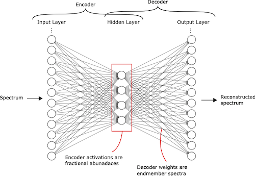
Figure 1: Schematic view of an autoencoder used for spectral unmixing.
3 Results and Conclusion
The signal decomposition techniques provide strong evidence for the presence of detectable mineralogical signals within the data, and the number of signal components estimated from PCA are consistent with the estimates from clustering.
PCA, ICA, and the abundance maps produced by the trained autoencoders all appear to convincingly replicate features of the surface topography. Figure 2 shows an example of this, comparing the quicklook image for phyllosilicates (a false colour RGB image constructed from wavelengths using spectral parameters; Viviano-Beck et al., 2014) to one of the produced abundance maps. This provides strong evidence that these methods have learnt mineralogically significant spectra, and that the autoencoders have learnt a physically plausible approximation to the LMM. This is despite the fact that at no spatial information is provided at any point to any of these methods – their results are purely based on spectral information.
Hence, when combined with methods to estimate the number of endmembers present, one can construct an unsupervised end-to-end linear unmixing model using autoencoders, that learns to identify physically plausible mineralogical endmembers. Once trained, this pipeline will allow the large number of CRISM data sets to be characterised and abundances mapped over the surface of the planet. This method is also extendable to any kind of planetary hyperspectral imaging, allowing simple mineralogical mapping on an unprecedented scale.
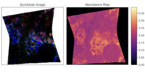
Figure 2: Quicklook image for phyllosilicates (a false colour RGB image made using spectral parameters; Viviano-Beck et al., 2014) alongside one of the produced abundance maps.
References
Guo, R., et al. (2015). Hyperspectral image unmixing using autoencoder cascade. In 2015 7th Workshop on Hyperspectral Image and Signal Processing: Evolution in Remote Sensing (WHISPERS), volume 2015-June, pages 1–4. IEEE.
Liu, Y., et al. (2016). End-member identi- fication and spectral mixture analysis of CRISM hy- perspectral data: A case study on southwest Melas Chasma, Mars. Journal of Geophysical Research: Planets, 121(10):2004–2036.
Murchie, S., et al. (2007). Compact Reconnaissance Imaging Spectrometer for Mars (CRISM) on Mars Reconnaissance Orbiter (MRO). Journal of Geophysical Re- search, 112(E5):E05S03.
Palsson, B., et al. (2018). Hyperspectral Unmixing Using a Neural Network Autoencoder. IEEE Access, 6:25646–25656.
Palsson, F., et al. (2017). Neural network hyperspec- tral unmixing with spectral information divergence objective. In 2017 IEEE International Geoscience and Remote Sensing Symposium (IGARSS), pages 755–758. IEEE.
Viviano-Beck, et al. (2014). Revised CRISM spectral parameters and summary products based on the currently detected mineral diversity on Mars. Journal of Geophysical Research E: Planets, 119(6):1403–1431.
Zhang, X., et al. (2018). Hyperspectral Unmixing via Deep Convolutional Neural Networks. IEEE Geoscience and Remote Sensing Letters, 15(11):1755–1759.
How to cite: Hipperson, M., Waldmann, I., Grindrod, P., and Nikolaou, N.: Mapping Mineralogical Distributions on Mars with Unsupervised Machine Learning, Europlanet Science Congress 2020, online, 21 Sep–9 Oct 2020, EPSC2020-773, https://doi.org/10.5194/epsc2020-773, 2020.
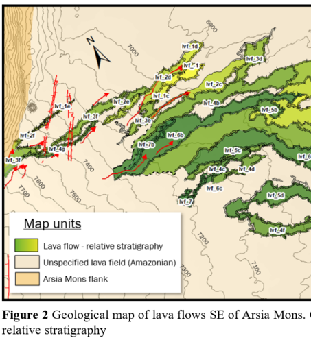
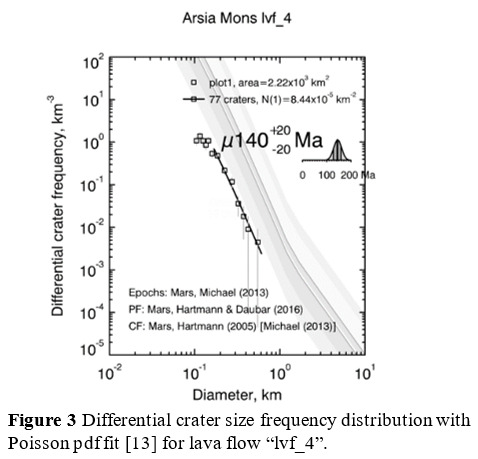
Introduction: The Tharsis dome is the main volcanic province on Mars. Being the locus of volcanism since at least the lower Hesperian, the age of emplacement and succession of its lava flows gives insights onto the thermal evolution of the planet since that time. Late Amazonian volcanic activity has taken the form of a large number of long and narrow lava flows, the vast majority of which unmapped to date. Mapping them is critical to characterize the recent dynamics of the Tharsis volcanism and relationships with tectonic activity. We focus on a group of fresh-looking lava flows located SE of Arsia Mons (Fig. 1). We map individual flows and determine their crater retention age, correlate with stratigraphy.

Geological Setting: Arsia Mons is the southernmost shield volcano of the Tharsis Montes. The edifice is ~400 km wide and rises 10 km above the surrounding topography. Its eruptive history includes explosive and effusive episodes [1]. The youngest episodes are thought to have occurred within the caldera and in the southern rift zone, forming a large fan-shaped lava aprons at 130 Ma [2,3]. Mapping of individual lava flows around vents [4] constrains the intra-caldera activity between 200-300 Ma and 90-100 Ma, with a peak at 150 Ma. The SE lava field (Fig. 1) was previously dated using HRSC data, and inferred to be 189 Ma [3].
Dataset and methods: Individual lava flows are mapped based on CTX images (6 m/px), THEMIS Night and Day-IR imagery (~100 m/px), and MOLA shots, and their succession is established using cross-cutting and stratigraphic relationships.
Absolute ages are estimated using automated crater detection and counting based on machine learning technique [5]. This method was favoured over manual counting because of time efficiency on large surface areas, such as total extents of lava flow. The algorithm was trained on THEMIS images where database for craters >1 km already exists [6]. The algorithm is applied to CTX mosaic from Murray Lab [7] to detect impact craters of diameter >100 m. A second algorithm based on cluster analysis is used to clean clusters of secondary impact craters. Each crater detection is then checked manually by visual inspection. Crater ages and errors are derived from crater size frequency distribution plots using Craterstats II [8] and Hartmann’s chronology system [9].
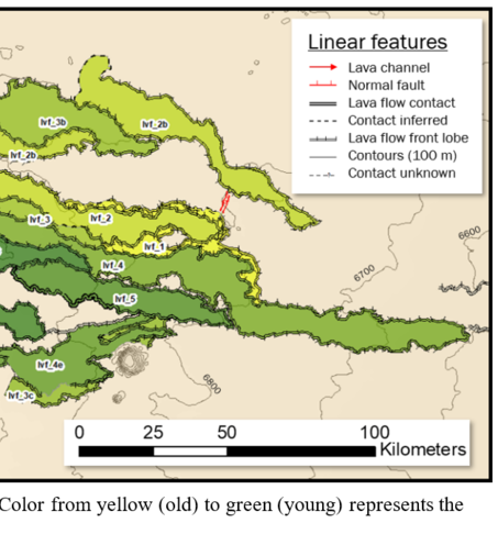
Results: We have mapped 37 individual lava flows and sorted them with respect to their stratigraphic relationships (Fig. 2). Flow length and width are in the range 20-300 km, and 0.7-21 km. Flows have typically a rugged surface with sometimes a medial channel system, while others display a smoother texture and wider extent.
The flows originate from the southern lava apron of Arsia Mons. The flowing direction is toward ESE, the direction of the current regional slope of the Tharsis dome. In the NW, they overprint SW-NE-trending grabens, but are cut by other normal faults from the same graben system, implying syn-tectonic volcanism. The total number of craters retrieved by the counting algorithm and kept after visual inspection is 948. The age of 23 flows could be obtained. They range from 200±50 Ma to 54±20 Ma, with 80% of lava flows between 60 and 160 Ma. In the SE, the longest lava flows lie on a 470±100 Ma older flow.
Discussion and perspectives: The obtained ages span 150 million years, with an apparent peak age at 150 Ma. This age corelates with the 150 Ma peak eruption age within the caldera [4]. It has been argued that a transition from explosive to effusive style occurred at Arsia Mons 200 Myrs ago [4]. Our results confirm that after effusive volcanism resumed, volcanic activity at Arsia Mons was not restricted to the caldera. Activity centered at the caldera and the southern flank followed a several hundred million years hiatus after main-flank building activity already noted by previous studies [3,4]. Crosscutting relationships between lava flows and bounding faults of concentric grabens indicate that extensional tectonics was coeval with some of the eruptions.
Length compared to width suggests lavas of mafic compositions. Texture pattern visible in CTX shows similarity with flows located further SW and NE of Daedalia Planum and dated 100 Ma [10]. The bright and rugged textures indicate differences in viscosity, similarly to basaltic flows found on the flanks of terrestrial shield volcanoes (aa’ and pahoehoe texture – e.g. [11]).
Morphometric study based on high-resolution digital terrain models will help confirm this interpretation and infer viscosity [12], a first step towards understanding the dynamics of the most recent eruptions at Arsia Mons.
Acknowledgments: This work is supported by the TEAM program of the Foundation for Polish Science (TEAM/2016-3/20), co-financed by the European Union under the European Regional Development Fund. This study is also supported by Europlanet 2024 RI's GMAP project.
References: [1] Ganesh I. et al. (2020) J. Volcanol. Geotherm. Res., 360. [2] Neukum G. et al. (2004) Nature, 432, 971-979. [3] Werner S.C. (2009), Icarus, 201, 44-68. [4] Richardson J.A. et al. (2017), EPSL, 458, 170-178. [5] Benedix, G. K. et al. (2020) Earth and Space Science 7, no. 3 [6] Robbins S. (2012), JGR, 117(E). [7] Dickson J.L. (2018), LPSC, Abstract #2480. [8] Michael G. G. and Neukum G. (2010) EPSL, 294, 223–229. [9] Hartmann W. K. (2005) Icarus, 174, 294–320. [10] Crown, D. A., & Ramsey, M. S. (2017). J. Volcanol. Geotherm. Res., 342, 13-28. [11] Holcomb, R. T. (1987) US Geol. Surv. Prof. Pap, 1350(1), 261-350. [12] Kolzenburg S. et al. (2018), J. Volcanol. Geotherm. Res., 357, 200-212. [13] Michael G. G (2016) Icarus 277:279–285
How to cite: Tesson, P.-A., Mège, D., Lagain, A., and Gurgurewicz, J.: Late Amazonian lateral lava flows coeval with caldera eruptions at Arsia Mons, Europlanet Science Congress 2020, online, 21 Sep–9 Oct 2020, EPSC2020-710, https://doi.org/10.5194/epsc2020-710, 2020.
The quantity, quality, and type of available datasets on Mars have improved in the last couple of decades. Context Camera (CTX) (Malin et al., 2007) on board the NASA Mars Reconnaissance Orbiter (MRO) provides a global coverage with an average resolution of 6 meters/pixel while the High Resolution Imaging Science Experiment (HiRISE) on board MRO (McEwen et al., 2007) allows up to 30 cm/pixel analyses at the local scale. These data allow at places also the DTM generation, but extensive topographic reconstructions at an average scale of 50 meters/pixel are possible using the High Resolution Stereo Camera (HRSC) on board of ESA Mars Express (MEX) (Neukum et al., 2004). Moreover compositional constraints can be provided by the spectral data coming from Observatoire pour la Minéralogie, l’Eau, les Glaces, et l’Activité (OMEGA) on board MEX and from Compact Reconnaissance Imaging Spectrometer for Mars (CRISM) on board the NASA Mars Reconnaissance Orbiter (MRO) (Murchie et al., 2007).
These relatively recent datasets coupled with the older datasets and Geographical Information Systems (GIS) provide an impressive suite of tools to develop meaningful planetary geological maps. In principle, these new data allow to add to the traditional geomorphological or chronostratigraphic mapping approaches, also a geological map approach somewhat akin to the one well-known on Earth, although, a ‘true’ geological map should be based on the lithological characters of the mapped units; using tone, texture, absence/presence of sedimentary structure, and, if possible, compositional hints to define the units, may represent an adequate ‘planetary perspective’, obviously in addition to the stratigraphic position within the succession. This map approach has the advantages to be relatively objective (and so potentially more useful for geological context analyses) and to represent the stratigraphic complexity within a region. This approach is complementary to the more interpretative (because it includes the processes/environments of formation of the different features) one of the geomorphological maps, which has the obvious advantage to describe the environments/processes active in the region.
In the framework of the GMAP (Geologic MApping of Planetary bodies) project, we present here an attempt to merge these two cartographic products taking advantage of GIS-based tools. Moreover, we aim at testing, where possible, the Earth-born symbols designed for the Geological Map of Italy (ISPRA, 2009, 2018) to try to make the ‘language’ of geological maps as uniform as possible. In order to perform these analyses, we selected a series of putative fluvio-lacustrine landforms located in Holden crater, along the south-eastern inner rim (coordinates 26.9°S-33.5°W). The geological map allowed to distinguish several units separated by unconformities. In particular, the Impact unit, equivalent to the one recognized by Tanaka et al. (2014) is nonconformably covered by the materials located inside the crater and along the crater rim. These materials can be distinguished in two groups separated by a disconformity, the first characterized by a relatively large lateral extension of the units and the second by a scattered appearance of the units. Within the first group, a disconformity separates a lower part from the upper part of the succession. The geomorphological map allows to genetically interpret these units, defining: i) a first impact stage, correspondent to the emplacement of Holden crater, ii) a ‘water-related’ phase (correspondent to the lower group of the geological map), and iii) an aeolian phase made of mega-ripples and dunes (correspondent to the upper group of the geological map). The ‘water-related’ phase can be further divided in a fluvio-lacustrine and a glacial phase.
We propose the realization of a unique geologic and geomorphologic product that includes a polygon layer with the geological units map described above, a linear layer with the unit contacts (i.e., stratigraphic characterization), and a linear shapefile with tectonic features and geomorphological interpretations. The polygonal units’ layer might be also suitable to subdivide the units in lower-order ranked units, using appropriate fields (i.e., formation/members on Earth). This approach might be best suited for projects developed at the local scale, similar to what is done on Earth, while a chronostratigraphic approach is more fitting and recommended at the regional and global scale. We will identify a possible set of graphical symbols describing the surface features, locating potential limits in current GIS symbology implementation.
The GMAP project represents an opportunity to share our experience and to collect current practices in planetary and terrestrial geological and geomorphological mapping, identifying what elements are still lacking and need to be discussed or developed.
References
ISPRA (2009) - Carta Geologica d’Italia. Guida alla rappresentazione cartografica. Modifiche e integrazioni ai Quaderni 2/1996 e 6/1997. Roma, pp. 166
ISPRA (2018) - Carta Geomorfologica d’Italia. Guida alla rappresentazione cartografica. Modifiche e integrazioni al Quaderno 4/1994. Roma, pp. 95
Malin, M. C., J. F. Bell, B. A. Cantor, M. A. Caplinger, W. M. Calvin, T. R. Clancy, K. S. Edgett, L. Edwards, R. M. Haberle, and P. B. James (2007), Context camera investigation on board the Mars Reconnaissance Orbiter, Journal of Geophysical Research: Planets(1991–2012), 112(E5).
McEwen, A. S., E. M. Eliason, J. W. Bergstrom, N. T. Bridges, C. J. Hansen, A. W. Delamere, J. A. Grant, V. C. Gulick, K. E. Herkenhoff, and L. Keszthelyi (2007), Mars reconnaissance orbiter’s high resolution imaging science experiment (HiRISE), Journal of Geophysical Research: Planets (1991–2012), 112(E5).
Murchie, S. et al. (2009), Evidence for the origin of layered deposits in Candor Chasma, Mars, from mineral composition and hydrologic modeling, Journal of Geophysical Research: Planets, 114, E00D05, doi:10.1029/2009je003343.
Neukum, G, R Jaumann, and H. the and Team (2004), HRSC—The High Resolution Stereo Camera of Mars Express, European Space Agency Special Publication, SP-1240, 17–35.
Tanaka, K., J. Skinner, J. Dohm, R. Irwin, E. Kolb, C. Fortezzo, T. Platz, G. Michael, and T. Hare (2014), Geologic map of Mars, USGS Scientific Investigations Map 3292, doi:10.3133/sim3292.
How to cite: Pondrelli, M., Frigeri, A., Marinangeli, L., Di Pietro, I., Pantaloni, M., Pozzobon, R., Nass, A., and Rossi, A. P.: Geological and geomorphological mapping of Martian sedimentary deposits: an attempt to identify current practices in mapping and representation, Europlanet Science Congress 2020, online, 21 Sep–9 Oct 2020, EPSC2020-232, https://doi.org/10.5194/epsc2020-232, 2020.
Crommelin Crater is a ~90km impact crater, located at 349.8° E and 5.1° N in Arabia Terra (Mars). This particular region displays a pervasive water and fluid activity fingerprint, made of several sulphate-bearing minerals, recorded both in Arabia and the nearby meridian planum and light albedo fine-layered deposits. These, informally named ELD (equatorial layered deposits [1, 2]) can be found both within craters and in the surrounding plateaus, and can range from 10 m to more than 1 km of thickness [1]. Indeed, several km-thick bulges made by ELDs can be seen within several craters of Arabia, among which the Crommelin Crater [1].
Its bulge is slightly elliptical in shape (50*30 km) covering almost more than half the size of the entire crater, with the surroundings of the bulge encompassed by gently folded ELDs. In order to investigate the possible origin of the bulge and of the folding we firstly performed a geological and structural mapping on a mosaic of CTX orthoimages at 6m/pixel (Context Camera onboard MRO [3]) and DEMs (Digital Elevation Models).
For this purpose we created a merged DEM of the whole crater area based on multi-resolution DEMs by means of CTX DEMs at 18 m (covering 2/3 of the crater), HRSC DEMs with 100 m and the final data gaps covered by MOLA MEGDR (Mars Orbiter Laser Altimeter Experiment Gridded Data Records [4]) data with 463 m of grid spacing respectively. From the geologic map, scaled 1:160.000, we could see that the bulge units occupy a lower stratigraphic level than the surrounding ELDs. These appear heavily eroded and dismantled with sharp contact at the base of to the bulge. We extracted ELD dip and strike measurements and combined them with the mapping of the prominent ELD strata: this way we were able to carry out a structural interpretation and to mark the position of inferred fold axes. Cross sections were defined crosscutting the strata orthogonally to their strike and topographic profiles together with all relevant information, such as inferred fold axes, intersecting bedding traces and local bedding attitude, were automatically computed for the chosen section traces by MOVE software with the aid of the DEM; the geologic interpretation was afterwards carried out in each of the cross-sections. The structural analysis highlighted the presence of gently folded strata whose axial planes appear concentric with respect to the bulge. Km-size symmetric folds sets are visible on the western sector, whereas asymmetric folds with radial outwards vergence are visible on the northwestern sector, appearing more pronounced in the proximity of the bulge. In the southern sector, a sequence of elliptical basins with inward dipping strata and major axis concentric to the bulge suggest a dome-basin interference pattern of folding. In order to further investigate the folded geometries and the structural setting, we approached the problem in 3D in MOVE software. By interpolating the same stratigraphic horizons across 13 interpreted cross-sections of the folded strata of the ELD unit in the western ans southern crater sectors, we reconstructed the full 3D geometry of deformed strata and built 3D ribbons of the main geologic contacts. The overall geostructural observations and the 3D reconstruction point towards the idea of a bulge uplift after the deposition of the surrounding layered deposits, that have caused fold sets typical of a diapiric phenomenon.
Acknowledgments: This research was supported by European Union’s Horizon 2020 under grant agreement No 776276- PLANMAP.
References:
[1] Pondrelli, M., Rossi, A.P., Le Deit, L., Fueten, F., van Gasselt, S., Glamoclija, M., Cavalazzi, B., Hauber, E., Franchi, F., Pozzobon, R., 2015. Equatorial layered deposits in Arabia Terra, Mars: facies and process variability. Geol. Soc. Am. Bull. https://doi.org/10. 1130/b31225.1.
[2] Hynek, B.M., Arvidson, R.E., Phillips, R.J, 2002. Geologic setting and origin of Terra Meridiani hematite deposit on Mars. J. Geophy. Res. Planet. 107 (E10), 18 -11-18-14.
[3] Malin, M.C., Bell, J.F., III, Cantor, B.A., Caplinger, M.A., Calvin, W.M., Clancy, R.T., Edgett, K.S., Edwards, L., Haberle, R.M., and James, P.B., 2007, Context Cam- era investigation on board the Mars Reconnaissance Orbiter: Journal of Geophysical Research, v. 112, E05S04, doi: 10 .1029 /2006JE002808 .
[4] Smith, D.E., Zuber, M.T., Solomon, S.C., Phillips, R.J., Head, J.W., Garvin, J.B., Banerdt, W.B., Muhleman, D.O., Pettengill, G.H., Neumann, G.A., Lemoine, F.G., Abshire, J.B., Aharonson, O., Brown, C.D., Hauck, S.A., Ivanov, A.B., McGovern, P.J., Zwally, H.J., and Duxbury, T.C., 1999, The global topography of Mars and implications for surface evolution: Science, v. 284, p. 1495–1503, doi: 10 .1126 /science .284 .5419 .1495 .
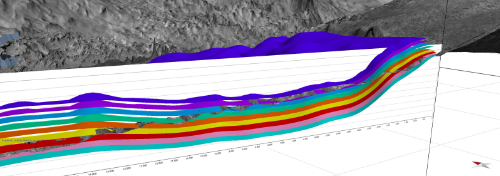
Figure 1: example of the reconstructed 3D layers in western Crommelin, in section view
How to cite: Pozzobon, R., Pesce, D., and Massironi, M.: 3D geomodel of the deformed deposits in Crommelin Crater (Mars), Europlanet Science Congress 2020, online, 21 Sep–9 Oct 2020, EPSC2020-770, https://doi.org/10.5194/epsc2020-770, 2020.
Modern and ancient fluvial-deltaic systems on Earth contain highly diverse ecosystems in all terrestrial climates. Fluvial and lacustrine deposits have been discovered on Mars by the NASA Mars Science Laboratory rover Curiosity, and may be present in Oxia Planum, where the ESA/ROSCOSMOS ExoMars rover Rosalind Franklin is set to land in 2023. The primary aim of the ExoMars mission is to search for signs of past and present life on Mars. Whilst fluvio-deltaic-lacustrine sandstones and mudstones are high priority targets for sampling and drilling, it is important to obtain information on the palaeoenvironmental context of these deposits during mission exploration.
The geometries of sedimentary structures and distribution of sedimentary facies within fluvial deposits provide information which can be used to reconstruct the geometries and flow parameters of these ancient systems. This provides us with quantitative means with which to make inferences on the ancient climate of Mars, and aids decision making with regards to rover science operations. Here we present a detailed quantitative 3D analysis of fluvial sedimentary architecture on Mars using rover image data. We used the 3D visualization software tool PRo3D1 to render the Shaler outcrop, observed at Yellowknife Bay by the NASA Mars Science Laboratory Rover, Curiosity2, as a scaled 3D textured model using the PRoViP 3D vision processing software3, and to map out key sedimentological features in order to characterize their geometry and dimensions, following existing facies descriptions4 .
Mastcam data taken from different rover locations was processed into 3D surfaces and spatially matched to Navcam stereo-panoramas to create a digital outcrop model (DOM). The Shaler DOM was constructed using 17 Mastcam stereo-panoramas taken on Sols 120-121 and 309-324. A 30 m x 13 m area of the NE-SW trending outcrop was analysed. Sedimentary facies, key bounding surfaces and sedimentary structures were mapped out on the DOM (Fig. 1) and the dip and strike of lithological boundaries, key bounding surfaces, and cross-laminations were measured directly from the DOM. Apparent widths and thicknesses of the layers and cross-lamination sets were measured. Regularly spaced, sedimentary logs were collected and matched to illustrate the detailed internal structures of the outcrops analysed. Four types of sedimentary structures were identified; low-angle cross strata dipping to the SE (Fig. 2), ~ 50 cm thick; convex up, sub-parallel undulating laminations forming structures with 20-40 cm amplitude and 2 m wavelength; single sets of trough cross-laminations and compound, stacked cosets of trough cross-laminations, with thicknesses on average 9 cm, and yielding a common palaeoflow direction to the NE and SW. These data allow us to reconstruct the internal architecture of a fluvial bar-form which forms the Shaler outcrop, and quantify the key geometries and their spatial relationships in three-dimensions. These data are highly useful in providing context and relative timings for environmental reconstruction.
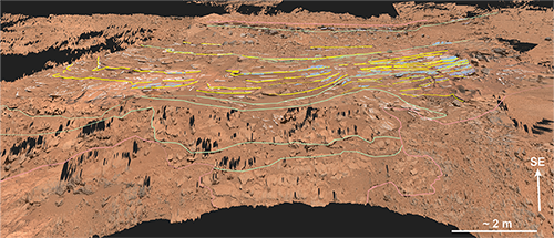
Figure 1. Line interpretation of Shaler in PRo3D, showing the lithological boundaries (pink lines), facies assocation boundaries (green lines), accretion surfaces (yellow lines), layer contacts (white lines), cross-lamina sets (blue lines) and undulatory convex up bedforms (green lines).
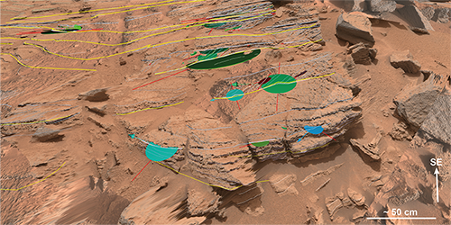
Figure 2. Detailed view of stacked sets of cross-laminations in the southwestern part of the Shaler outcrop.
1. Barnes et al., 2018, Geological Analysis of Martian Rover‐Derived Digital Outcrop Models Using the 3‐D Visualization Tool, Planetary Robotics 3‐D Viewer—PRo3D. Earth and Space Science.
2. Grotzinger et al., 2014, A Habitable Fluvio-Lacustrine Environment at Yellowknife Bay, Gale Crater, Mars. Science
3. Paar et al., 2015, PRoViDE: Planetary Robotics Vision Data Processing and Fusion. European Planetary Science Congress 2015.
4. Edgar et al., 2017, Shaler: in situ analysis of a fluvial sedimentary deposit on Mars. Sedimentology.
How to cite: Barnes, R., Gupta, S., Paar, G., Bauer, A., Ortner, T., and Traxler, C.: Three-dimensional reconstruction and quantification of fluvial-deltaic sedimentary deposits in Gale crater, Mars, from rover-derived Digital Outcrop Models., Europlanet Science Congress 2020, online, 21 Sep–9 Oct 2020, EPSC2020-821, https://doi.org/10.5194/epsc2020-821, 2020.
1 Introduction & Scope
The remarkable success of deep learning (DL) for object and pattern recognition suggests its application to autonomic target selection of future Martian rover missions, to support planetary scientists and also exploring robots in preselecting possibly interesting regions in imagery, increase the overall scientific discoveries, and to speed-up the strategic decision-making.
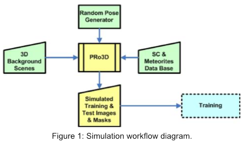
Deep learning requires large amounts of training data to work reliably. Many different geologic features are to be detected and to be trained for in a DL-systems. Past and ongoing missions such as the Mars Science Laboratory (MSL) do neither provide the necessary volume of training data nor existing “ground truth”. Therefore, realistic simulations are required. The scheme and workflow of the Mars-DL simulation is depicted in Figure 1.
Realistic simulations are based on accurate 3D reconstructions of the Martian surface, which are obtained by the photogrammetric processing pipeline PRoVIP [1]. The resulting 3D terrain models can be virtually viewed from different angles and hence can be used to obtain large volumes of training data.
2 Shatter Cones
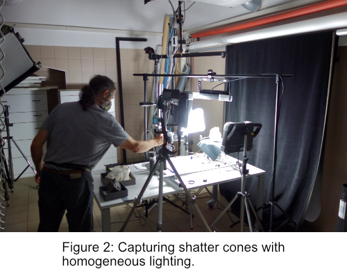
For Mars-DL it was decided to focus on shatter cones (SC), which are macroscopic evidence of shock metamorphism and form during meteorite impact events [2]. Shatter cones take on a variety of sizes and shapes depending mainly on the rock type, but all of them have distinctive fan-shaped “horsetail” structures that resemble striations, which makes them well-suitable objects to train a DL-system and assess its detection reliability. Due to their rare presence in real imagery, we place textured 3D models of SCs into the real context of a Martian surface region. A 3D capturing and reconstruction campaign provided a series of 3D models from SCs taken from actual terrestrial impacts (Figure 2).
They have sufficient geometric and texture resolutions to preserve characteristic features. To allow shading of SCs the texture was captured with homogeneous lighting to obtain a pure albedo map without any prebaked lighting. High resolution DTMs (Digital Terrain Models) of Martian surfaces usually have an image texture being derived from rover instrument imagery. Their prebaked lighting effects such as shading, shadows and specular highlights are determined by the sun’s direction at capturing time, obtained from SPICE. For a shatter cone to perfectly blend into the scene, it first needs to be shaded from the same illumination direction and second it needs to cast a shadow from the same angle as found in the original background surface.
Many shatter cones from terrestrial sites have a contact surface, where they were broken or cut from the outcrop and museum specimens often bear a label. This surface must not be visible in training images (although broken cones exist in impact deposits as well), and are marked by a vector as part of the meta-data of the 3D model to keep them invisible during automatic positioning.
3 Simulation with PRo3D
Planetary scientists can explore high-resolution DTMs with a dedicated viewer called PRo3D [3]. Fluent navigation through a detailed geospatial context allows visual experience close to field investigations. Therefore, PRo3D offers much of the required functionality to generate large volumes of training images.
PRo3D was extended for batch rendering to enable mass-production of training data. It accepts commands from a JSON file that defines many different viewpoints from which to render different types of images. The training of DL systems also demands masks for the shatter cones and depth images. For both, special GPU shaders were implemented.
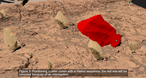
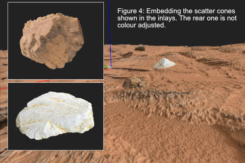
The automatic random positioning of shatter cones is also controlled by JSON commands. We calculate positions for a given viewpoint region with a Halton sequence, which guarantees an even distribution. The size and rotation of each SC is randomly modified within given ranges, observing visibility constraints mentioned above. Axis-aligned bounding boxes of SCs are used to determine how deep they penetrate into the surface and allow efficient collision detection between SCs. Intersections are avoided by removal of individual SCs (Figure 3). To enhance realism, SCs are color adjusted to the image texture of the surrounding environment and shaded with the appropriate illumination direction obtained from the corresponding SPICE kernels (Figure 4).
We present an efficient way to generate large amounts of images for the training of DL systems to support autonomous scientific target selection in future rover missions. It is based on available high-resolution Martian surface reconstructions and newly created shatter cone models. The viewer PRo3D, developed for planetary science explorations, was extended for the efficient mass simulation of different DL training sets.
Future work includes the design of a shader that combines shadows cast from SCs with the image texture of the surrounding surface and a fully automatic color adjustment.
References
[2] French B.M., and Koeberl C. (2010) The convincing identification of terrestrial meteorite impact structures: What works, what doesn't, and why. Earth-Science Reviews 98, 123–170.
[3] Barnes R., Sanjeev G., Traxler C., Hesina G., Ortner T., Paar G., Huber B., Juhart K., Fritz L., Nauschnegg B., Muller J.P., Tao Y. and Bauer A. Geological analysis of Martian rover-derived Digital Outcrop Models using the 3D visualisation tool, Planetary Robotics 3D Viewer - Pro3D. In Planetary Mapping: Methods, Tools for Scientific Analysis and Exploration, Volume 5, Issue 7, pp 285-307, July 2018.
Acknowledgments
This abstract presents the results of the project Mars-DL, which received funding from the Austrian Space Applications Programme (ASAP14) financed by BMVIT, Project Nr. 873683.
How to cite: Traxler, C., Fritz, L., Nowak, R., Paar, G., Koeberl, C., Bechtold, A., Garolla, F., and Sidla, O.: Simulating rover imagery to train deep learning systems for scientific target selection, Europlanet Science Congress 2020, online, 21 Sep–9 Oct 2020, EPSC2020-566, https://doi.org/10.5194/epsc2020-566, 2020.
Introduction: The Apollo 15 landing site is one of the calibration points for the lunar cratering chronology, which compares crater size-frequency distribution (CSFD) measurements to lunar sample ages [e.g., 1-6]. Following our series of studies [7-10] of the lunar chronology using recent lunar mission and sample analysis data [11-15], we produced new detailed geological maps of Apollo 15 landing site and used these to define homogeneous areas for measuring CSFDs of the geological units where samples were collected.
Methods: We used LROC Wide Angle (WAC; 100 m/pixel) and Narrow Angle Camera (NAC; ~0.5 m/pixel) data [11] with incidence angles between 55-80°, SELENE (Kaguya) image data, a LOLA/SELENE merged digital elevation model (DEM) [12], Clementine [13] and Kaguya Multiband Imager (MI) data [16] for geological mapping. The CSFDs were measured on the identified geological units by using CraterTools [17] in ArcGIS, and the gained values were plotted in Craterstats [18] using pseudolog binning, in cumulative and relative plot. Randomness analyses [19] were used to identify and avoid secondary crater chains and clusters. The new N(1) values will be correlated with recently determined sample ages [20] to obtain new calibration points.
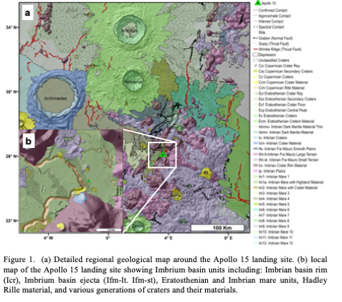
Geological Events: The Apollo 15 landing site lies east of the Hadley rille near the rim of the Imbrium basin. The mapped area contains the Imbrium basin rim (Icr), Imbrium basin ejecta (Ifm-lt, Ifm-st, and Ifs, mapped on the basis of topographical differences), and Imbrian plains (Ip). The valley is filled with various mare units belong to Eratosthenian- and Imbrian-aged mare units [21], which are resurfaced by the ray and secondary crater materials from both Autolycus and Aristillus craters [22,23]. The network of rilles in vicinity belongs to different ages.
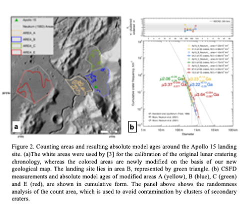
CSFD Measurements: The new geological map was used to modified Neukum’s (1983) selected count areas A, B, C, and E, and to measure CSFDs in these areas using LRO and Kaguya image data. Areas A and B lie on the same mare unit (Im1) and have N(1) values of 2.99x10⁻³ km-2 and 2.98x10⁻³ km-2, The landing site lies in Area B. Area C consists of various geological units and we gain N(1) value of 1.72x10⁻³ km-2, which may represent young crater material. Similarly, Area E also has two N(1) values of 3.55x10⁻³ km-2 and 7.88x10⁻³ km-2, representing two mare units.
Neukum (1983)[3] used an N(1) value of 3.2±1.1x10⁻³ km-2 measured on Area B, and sample age ~3.28 Ga for the lunar cratering chronology calibration [3]. The recent sample analyses determined ages of ~3.26 Ga for olivine normative basalts and ~3.35 Ga for quartz normative basalts [20].
Acknowledgements: WI and HH were funded by the German Research Foundation (Deutsche Forschungsgemeinschaft SFB-TRR170, subproject A2) and CvdB was supported by EU H2020 project #776276, PLANMAP
References: [1] Hartmann (1970) Icarus 13, 299-301. [2] Neukum et al. (1975) The Moon 12, 201-229. [3] Neukum (1983) NASA TM-77558. [4] Neukum et al. (2001) Space Sci. Rev. 96, 55-86. [5] Robbins (2014) EPSL 403, 188-198. [6] Stöffler et al. (2006) Rev. Min. Geochem. 60, 519-596. [7] Iqbal et al (2019) Icarus 333, 528-547. [8] Iqbal et al (2018) LPSC 49, 1002. [9] Iqbal et al (2019) LPSC 50, 1005. [10] Hiesinger et al (2020) LPSC 51, this conference [11] Robinson et al (2010) Space Sci. Rev. 150, 81-124. [12] Barker et al. (2016) Icarus 273, 346-355. [13] Pieters et al. (1994) Science 266, 1844-1848. [14] Ohtake et al (2013) Icarus 226, 364-374. [15] Nemchin et al (2018) LPSC 49, 1936. [16] Lemelin et al (2016) LPSC 47, 2994. [17] Kneissl et al. (2011). PSS 59, 1243-1254. [18] Michael et al. (2016) Icarus 277, 279-285. [19] Michael et al. (2012) Icarus 218, 169-177. [20] Snape et al (2019) GCA. 266, 29-53. [21] Hiesinger et al (2000) JGR 105, 29239-29275. [22] Howard (1971) USGS, I-723 [23] Carr et al (1971) USGS, I-723.
How to cite: Iqbal, W., van der Bogert, C., and Hiesinger, H.: Detailed Geological Studies and Absolute Model Ages of the Apollo 15 Landing Site, Europlanet Science Congress 2020, online, 21 Sep–9 Oct 2020, EPSC2020-1091, https://doi.org/10.5194/epsc2020-1091, 2020.
On the southern hemisphere of the lunar farside lies the interesting Tsiolkovskiy crater that presents on its floor one of the few exposures of mare volcanism on the far side and an unusually well-shaped central peak.
Its morphology and the remotely-sensed detection of minerals such as olivine and Purest Anorthosite (PAN), make Tsiolkovskiy crater an area to be considered for a possible landing site for a rover-based exploration. With this objective we are carrying on a geological characterization of this crater.
Tsiolkovskiy crater (20.4° S, 129.1° E) is a Late Imbrian impact crater with an elliptical shape and a minor axis diameter of about 180 km [1, 2].
Over the crater floor rises a ~3 km-high particularly bright and well-preserved central peak surrounded by an exclusively dark and smooth mare deposit formed by multiple eruptive events [2]. Moreover, on the central peak have been detected PAN [3, 4] and olivine [5].
The above-mentioned characteristics highlight the scientific interest represented by Tsiolkovskiy crater as a main driver to characterize its interior as landing site and evaluate the possibility to safely plan route traverses for rovers.
Aiming to focus the strategy of exploration for a future lunar landing mission we are producing geological maps of the area in order to select locations of high interest and traverse paths for in-situ investigations and analysis in order to help unravel key scientific questions concerning the origin and evolution of the Moon, the structure and composition of the lunar crust and interior and the presence of volatiles and of minor and trace elements.
The geomorphological mapping of the impact crater has been carried out on the Lunar Reconnaissance Orbiter Wide Angle Camera [6] global mosaic with a resolution up to 100 m/pixel along with elevation data derived from the Lunar Orbiter Laser Altimeter and Kaguya Terrain Camera DEM merge [7] with an horizontal and vertical resolution respectively of about 59 m/pixel and 3-4 m.
The surface morphology mapping has then been coupled with the spectral mapping performed on the ~200 m/pixel false color composite (Red 750/415 nm; Green 750/1000 nm; Blue 415/750 nm) generated using the Clementine UVVIS [8] reflectance image.
Moreover, an high-resolution mapping is being produced on Lunar Reconnaissance Orbiter Narrow Angle Camera (NAC) [7] images along with NAC-derived DEMs both with a resolution of about 0.5 m/pixel.
From the geomorphological mapping (Fig. 1) have been distinguished the following crater floor (CF) and crater walls (CW) units:
- CF smooth material: very smooth and planar material with a sharp boundary with respect to adjacent materials,
- CF hummocky material: rough material reworked during the impact and CW debris,
- CF central peak: sharp and well-recognizable central peak morphology,
- CW smooth ponds: smooth material areas texturally discording with respect to the surrounding areas,
- CW steep scarps: exposed steep scarps with slopes >40°,
- CW rim: terraces and scarps made up by collapsed material.
The spectral mapping (Fig. 2), instead, has been performed on the basis of the different color of the units, associated to a different origin and composition of the materials. The mapping allowed the distinction of the following units:
- Fresher basalts: predominant yellow color, corresponding to most of the CF smooth material,
- Basaltic plain: predominant orange color, corresponding to the remaining CF smooth material unit,
- Noritic-anorthosite/troctolite: light blue color, mostly correlated to the CF central peak and CW steep scarps units,
- Anorthosite: blue color, mostly correlated to the CF central peak and CW steep scarps units,
- Mature highland soil: red color, corresponding to the CW rim, CW smooth ponds and CF hummocky material units.
Finally, in the area surrounding the central peak of Tsiolkovskiy crater is being produced an high-resolution geological mapping with the aim to better define the geological setting for a rover-based exploration. So far, the mapping allowed to highlight some interesting features such as mare rilles and wrinkle ridges in proximity to the peak.
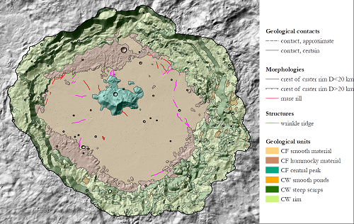
Fig. 1: Geomorphological mapping superposed on the hillshade generated from the Lunar Orbiter Laser Altimeter and Kaguya Terrain Camera DEM merge.
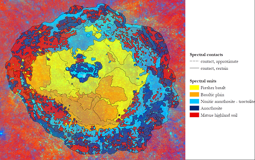
Fig. 2: Spectral mapping superposed on the Clementine UVVIS Color Ratio.
Here we presented the geomorphological and spectral mapping of Tsiolkovskiy crater performed so far. In the next future the high-resolution mapping will be completed and coupled with a spectral investigation by means of Chandrayaan-1’s Moon Mineralogy Mapper [9] data. Moreover, a radar investigation for the presence of deep structures, such as voids and lava pile emplacements, will be carried on by means of Kaguya Lunar Radar Sounder [10] data. To conclude, in order to perform a complete characterization of Tsiolkovskiy crater as a possible future landing site, we will perform a steepness and hazard analysis for the definition of the landing ellipses and route traverses for a rover exploration.
Acknowledgements
This research was supported by the European Union’s Horizon 2020 under grant agreement No 776276-PLANMAP.
References
[1] Whitford-Stark, J.L. & Hawke, B.R., XIII LPSC, pp. 861-862, 1982
[2] Pieters, C.M. & Tompkins, S., JGR, Vol. 104, pp. 21935-21949, 1999
[3] Ohtake, M. et al., Nature, Vol. 461, pp. 236-241, 2009
[4] Lemelin, M. et al., JGR: Planets, Vol. 120, pp. 869-8878, 2015
[5] Corley, L.M. et al., Icarus, Vol. 300, pp. 287-304, 2018
[6] Robinson, M.S. et al., Space Sci. Rev., Vol. 150, pp. 81–124, 2010
[7] Barker, M.K. et al., Icarus, Vol. 273, pp. 346-355, 2016
[8] Lucey, P.G. et al.,JGR, Vol. 105, pp. 20377-20386, 2000
[9] Pieters, C. M. et al., Current Science, Vol. 96, pp. 500-505, 2009
[10] Ono, T. et al., Space Sci. Rev., Vol. 154, pp. 145-192, 2010
How to cite: Tognon, G., Pozzobon, R., and Massironi, M.: Landing site characterization for Tsiolkovskiy crater, Europlanet Science Congress 2020, online, 21 Sep–9 Oct 2020, EPSC2020-581, https://doi.org/10.5194/epsc2020-581, 2020.
Abstract
In order to provide a dataset for a Virtual Reality environment for Astronaut training, 3D images of 1m/pixel of Aristarchus Crater has been produced using the CASP-GO software based on the NASA’s Ames Stereo Pipeline. In addition to the 3D images, to provide the best viewing quality, 50cm/pixel images with the least shadow are chosen to be terrain corrected with the topographical information. This research will show the selection of the images used in this dataset, their processing, and the current status of the 3D imaging datasets.
1. Introduction
The NASA ARTEMIS Programme is a human exploration programme carried out by NASA, US commercial spaceflight companies, ESA, JAXA, and CSA. The programme is the next step in establishing a sustainable human presence on the Moon amongst other goals. Aristarchus is a young crater with transient features which was previously selected as a site for the Apollo 18 mission and is one of the landing site candidates for the ARTEMIS mission. To provide a VR dataset for astronaut training for the mission, the best 3D image dataset is needed, which we currently lack. This dataset can be achieved using LROC-NAC, the current highest resolution and coverage on the Moon that has been operating continuously since 2009.
A fully automated multi-resolution Digital Terrain Model processing chain for Mars stereo imagery (ESA-HRSC, NASA-MRO/CTX and HiRISE) based on the Ames Stereo Pipeline [1] has been developed at UCL within The EU-FP7 iMars project (http://www.i-mars.eu) called CASP-GO[2]. CASP-GO utilises tie- point-based multi-resolution image co-registration [3], and the Gotcha [4] sub-pixel refinement method. Since the end of the project in March 2017, thousands of CTX, and tens of HiRISE and HRSC 3D products have been processed with CASP-GO and have been published through the ESAC Guest Storage Facility (GSF) [5].

Figure 1: Current Version of the Aristarchus Image Mosaics
2. Methods
Stereo pairs have been selected from the official LROC-NAC stereo pair list. However, as the stereo pairs on the list only covers roughly half of the crater and ends in 2018, a MatLab code was written to look for a new set of stereo pairs to fill the gaps using the LROC-NAC coverage shapefiles (https://ode.rsl.wustl.edu/moon/indextools.aspx?displaypage=footprint) information until 2 February 2020.
Other than the ASP core pre-processing, initial matching, subpixel matching, camera triangulation, and DTM generation, five additional workflows are used to improve the DTM quality in CASP-GO. MGM is employed from the latest ASP pipeline to improve DTM quality [6]. A wrapper is written to allow processing of LROC-NAC stereo pairs in CASP-GO.
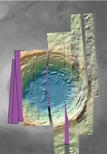
Figure 2: Current Coverage of Aristarchus Individual DTMs with remaining stereo pairs to process (purple)
3. Results
A base map was initially generated using the 20m/pixel Chang’E2 DTM [6] co-registered to the LOLA-SELENE 69m/pixel DTM product [7]. The 1m/ pixel DTMs are created using this DTM as a base for co-alignment using iterative closest point adjustment. Masks are created to crop out bad data, especially on the overlapping areas between multiple individual DTMs. Residuals are reduced by using the ISIS pc_align. The orthorectified 0.5-1m images are used as a reference alongside the Chang’E 2 orthorectified images and the LROC-WAC image to look for overlapping images with similar solar azimuth, phase, and solar elevation angles to produce 50cm/pixel images. The current mosaic is shown in Figure 1.
The resultant multi-resolution and bundle-adjusted co-registered 1m 3D models will be provided with a 0.5m mosaiced corrected image for employment with NASA Moontrek [7]. VR will be employed by NASA for astronaut training using these data for the ARTEMIS programme. These products will be made available through the ESA Guest Storage Facility once a peer review paper is accepted, the ESA-GSF is described elsewhere [8]. An example of a 3D view of the current version of the result is shown in Figure 3.

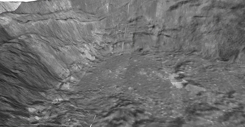
Figure 3: 3D View of images overlaid on Digital Terrain Models in QGIS 3D Map View
4. Summary and Future Work
In this research, a 1m/pixel Aristarchus DTM mosaic has been created using individual DTMs made using the UCL CASP-GO pipeline. A mosaic of images is being produced with the same viewing condition. A full assessment will be performed to provide the best quality DTM and ORI mosaics following the completion of the DTMs and the ORIs to help visualize the human mission to the moon. These 3D map products will be publicly released in the near future.
Acknowledgements
This work is funded by NASA Contract No. 1639009. Part of the research leading to these results has received partial funding from the European Union’s Seventh Framework Programme (FP7/2007-2013) under iMars grant agreement n˚ 607379. We thank Emily Law (NASA PDS) for helpful discussions and inputs.
References: [1] Beyer, R., et al. (2018), Earth and Space Science, vol 5(9), pp.537-548. [2] Tao, Y., J-P. Muller, Putri et al. (2018) PSS, Vol. 154, pp.30-58, [3] Tao, Y., Muller, et al. (2016), Icarus, vol 280, pp.139-157. [4] Shin, D. and J.-P. Muller (2012), Pattern Recognition, vol 45(10), pp.3795 - 3809. [5] Muller, J.-P. et al. (2019), Vol. 13, EPSC-DPS2019-1355-1. [6] Di, K et al. (2014). Planetary Geodesy and Remote Sensing, pp. 77–96. [7] Day, Schmidt, Law (2019) Vol. 13, EPSC-DPS2019-1154-1 [8] Barker, M.K. et al. (2016) Icarus, 273, 346–355.
How to cite: Putri, A. R. D., Chernetskiy, M., Tao, Y., and Muller, J.-P.: 3D Imaging of Aristarchus Crater for Human Exploration on the Moon, Europlanet Science Congress 2020, online, 21 Sep–9 Oct 2020, EPSC2020-617, https://doi.org/10.5194/epsc2020-617, 2020.
Please decide on your access
Please use the buttons below to download the presentation materials or to visit the external website where the presentation is linked. Regarding the external link, please note that Copernicus Meetings cannot accept any liability for the content and the website you will visit.
Forward to presentation link
You are going to open an external link to the presentation as indicated by the authors. Copernicus Meetings cannot accept any liability for the content and the website you will visit.
We are sorry, but presentations are only available for users who registered for the conference. Thank you.