Oral presentations and abstracts

Abstract

Observations from the Texas Echelon Cross Echelle Spectrograph (TEXES) on NASA’s IRTF and the VISIR instrument on the VLT are used to characterize the Saturn’s seasonal changes. Radiative transfer modelling (using NEMESIS [8]) provides the northern hemisphere temperature progression of the atmosphere over 10 years, both during and beyond the Cassini mission. Comparisons between imaging observations taken one Saturn year apart (1989-2018) show the extent of the interannual variability of Saturn’s northern hemisphere climate for the first time.

1. Introduction

With the culmination of Cassini's unprecedented 13-year exploration of the Saturn system in September 2017, and with no future missions currently scheduled to visit the ringed world, the requirement to build upon Cassini's discoveries now falls upon Earth-based observatories. Mid-infrared observations have been used to characterise features such as the extreme temperatures within an enormous storm system in 2011 [1,6], the cyclic variations in temperatures and winds associated with the 'Quasi-Periodic Oscillation' (QPO) in the equatorial stratosphere [2] and the onset of a seasonal warm polar vortex over the northern summer pole [3].

Saturn's axial tilt of 27º subjects its atmosphere to seasonal shifts in insolation [4], the effects of which are most significant at the gas giant's poles. The north pole emerged from northern spring equinox in 2009 (planetocentric solar longitude L_s=0º), and northern summer solstice in May 2017 (L_s=90º), providing Earth-based observers with their best visibility of the north polar region since 1987, with its warm central cyclone and long-lived hexagonal wave [5,6].

Studying these interconnected phenomena within Saturn's atmosphere (particularly those that evolve with time in a cyclic fashion) requires regular temporal sampling throughout Saturn's long 29.5-year orbit. We present here a showcase of research from the wealth of archived observations from both TEXES and VISIR obtained over the past decade.

1.1 Temperature progression

Methane (CH₄) is used to determine stratospheric temperatures due to its even distribution across the planet, as well as its well understood emissive behavior. Figure 1 shows the visible changes in the stratospheric and tropospheric conditions as seen by VISIR over 3 years; these images are representative of a range of filters between 7-20 µm, which can be stacked and inverted to derive the 3D temperature distribution in the upper troposphere and stratosphere. Using this technique, we probe changes in the atmospheric 3D temperature distribution across the planet disc in VISIR observations taken from April 2008 (L_s=343º) to July 2018 (L_s=102º); thereby discerning the spatial variability as well as temporal. VISIR observations concurrent with the Cassini/CIRS observations will be used to cross-check the time-series from Cassini, which can be extended beyond the end-of-mission with the newer VISIR observations. These profiles will provide a new measure of long-term temperature variability in the context of an established model.

1.2 Interannual Variability

Spectroscopic maps of the northern summer hemisphere from TEXES instrument on the IRTF collected in September 2018 have provided a unique opportunity, as they were acquired exactly one Saturn year apart from the 1989 observations of Gezari et al, (1989) [7], which were the first ever 2D images of Saturn in the mid-IR. Examining the differences in brightness temperatures and composition will indicate the extent of any interannual variation for Saturn’s northern hemisphere. This study will also provide unique insight into the timescale of the QPO which will be contrasted with a previously suggested biennial cycle [2]. The seasonal temperature progression measured in Section 1.1 also enables us to place this interannual variability in a wider context and provides further opportunity for insightful comparison with the comparatively shorter-term temperature variability.

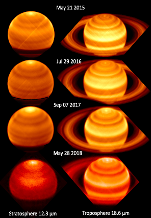
Figure 1: VISIR observations from P95-102 sensing the troposphere (right) and stratosphere (left).  Polar warming is evident in the stratosphere; but is considerably smaller than that seen during southern summer and in the historical record of the 1980s.  The warm polar hexagon is seen at the north pole, the first such observation from the ground. Work to remove residual striping is ongoing and has been successfully applied to the 2017 images. 2015-16 images have been published by Fletcher et al., 2017 [2].

Acknowledgements

This research is funded by a European Research Council consolidated grant under the European Union’s Horizon 2020 research and innovation program, grant agreement 723890. We would like to thank co-author Mael Es-Sayeh for his significant contribution to this research.

References

[1] Fletcher et al., 2012, Icarus 221, p560-586

[2] Fletcher et al., 2017, Nature Astronomy, 1, p765-770

[3] Fletcher et al. 2015, Icarus. 251, 131-153

[4] Fletcher et al., 2015, https://arxiv.org/abs/1510.05690

[5] Fletcher et al., 2008, Science. 319, 79-81

[6] Fouchet et al., 2016, Icarus, 277, p196-214

[7] Gezari et al., 1989, Nature, 342, 777–780

[8] Irwin et al. 2008, JQSRT 109:1136-1150

[9] Orton et al., 2008, Nature 453, p198

How to cite: Blake, J., Fletcher, L., Antunano, A., Melin, H., Roman, M., Es Sayeh, M., Donelly, P., Rowe-Gurney, N., King, O., Greathouse, T., and Orton, G.: Saturn’s Seasonal Atmosphere: Cassini CIRS contrasts to VLT and IRTF observations, Europlanet Science Congress 2020, online, 21 Sep–9 Oct 2020, EPSC2020-310, https://doi.org/10.5194/epsc2020-310, 2020.

To address questions about the driving mechanisms of Saturn's equatorial oscillation, our team at the Laboratoire de Météorologie Dynamique built the DYNAMICO-Saturn Global Climate Model to study tropospheric dynamics, tropospheric waves activity (Spiga et al. 2020) and equatorial stratospheric dynamics (Bardet et al. 2020) of Saturn. Previous studies (Guerlet et al. 2014, Spiga et al. 2020, Cabanes et al. 2020) have shown that our model produces consistent thermal structure and seasonal variability compared to Cassini CIRS measurements, mid-latitude eddy-driven tropospheric eastward and westward jets commensurate to those observed and following the zonostrophic regime, and planetary-scale waves such as Rossby-gravity (Yanai), Rossby and Kelvin waves in the tropical channel. Extending the model top toward the upper stratosphere allowed our model to produce an almost semi-annual equatorial oscillation with opposite eastward and westward phases. Associated temperature anomalies have a similar behavior than the Cassini/CIRS observations, but the amplitude of the temperature oscillation is twice smaller than the observed one. The absence of sub-grid-scale waves in the model produces an imbalance in eastward- and westward-wave forcing on the mean flow and could be an explanation to the irregularity in both the oscillating period and the downward rate propagation of the resolved Saturn equatorial oscillation.

To explore the impact of those small-scale waves on the spontaneous equatorial oscillation emerging in the DYNAMICO-Saturn GCM (Bardet et al. 2020), we add a sub-grid-scale non-orographic gravity waves drag parameterization in our model.
This parameterization is directly adapted from the stochastic terrestrial model of Lott et al. (2012). This formalism represents a broadband gravity wave spectrum, using the superposition of a large statistical set of monochromatic waves. As the time scale of the life cycles of gravity waves is much longer than the time step of our GCM, our parametrization can launch a few waves whose characteristics are randomly chosen at each time step. This stochastic gravity waves drag parameterization is applied in DYNAMICO-Saturn on all points of the horizontal grid.

A key parameter used in the non-orographic gravity waves drag parameterization is the maximum value of the Eliassen-Palm flux. The Eliassen Palm flux represents the momentum carried by waves that could be transferred to the mean flow. This value has never been measured in Saturn's atmosphere and it represents an important degree of freedom in the parameterization of gravity waves.

We performed several test simulations, lasting two Saturn years whose initial state is derived from Bardet et al (2020), with an horizontal resolution of 1/2° in longitude/latitude and a vertical resolution ranging between 3 bar to 1 μbar. For these test simulations, the maximum value of the Eliassen-Palm fulx is set to 10^-6, 10^-5, 10^-4 and 10^-3 kg m^-1 s^-2. 

Preliminary results show that the appropriate value of our main parameter is between 10^-5 and 10^-4 kg m^-1 s^-2. Eliassen-Palm flux value of 10^-3 kg m^-1 s^-2 demonstrates a too large impact: the equatorial oscillation is entirely vanished is this configuration. The simulation using the value of 10^-6 kg m^-1 s^-2 is equivalent to the control simulation without the gravity waves drag parameterization.  

The next step is to test other parameters, as phase velocity of the gravity waves, horizontal wavenumber, to understand how gravity waves impact the equatorial oscillation.

How to cite: Bardet, D., Spiga, A., Guerlet, S., Millour, E., and Lott, F.: Parameterizing gravity waves in the DYNAMICO-Saturn Global Climate Model to understand Saturn's equatorial oscillation, Europlanet Science Congress 2020, online, 21 Sep–9 Oct 2020, EPSC2020-601, https://doi.org/10.5194/epsc2020-601, 2020.

The delivery of enriched icy grains has been proposed as a mechanism to explain the enrichment of Jupiter with noble gases [1]. The enrichment with noble gases imposes constraints on the formation temperature of these grains, with Ar in particular only adsorbing to amorphous ice below 30K [2]. While significant consideration has been given to the formation conditions of the ices, the release of species as the grain migrates inward toward the forming planets has been given less thought. The desorption of the noble gases Ar, Kr and Xe trapped in amorphous ice occurs largely below 80K [3], while Jupiter formed at a temperature of 130K. [4] The composition of the icy grains thus changes from formation to deposition. The accretion and release processes are visualised in Figure 1.

The accretion and subsequent desorption of noble gas species alongside water into an enriched icy grain has been simulated using a Monte Carlo model. Assuming a tetrahedral structure of amorphous water ice, particles are deposited onto a predefined grid at temperatures sufficiently low to retain Ar. The temperature is subsequently increased up to 150K, capturing the temperature range relevant for giant planet formation. Previously reported experimental measurements of evaporation rates are used to benchmark the model and constrain the diffusion and evaporation rates of each noble gas species. The accretion and heating phases are shown in Figure 2, alongside the relevant physical processes. The desorption of each species from the ice is tracked during heating, and used to compute the temperature-dependent enrichment profile of the grain.

The Ar/Xe ratio of an icy grain simulated to form at 20K and heated up to 150K is shown in Figure 3. The higher thermal velocity of Ar causes the grains to initially be excessively enriched with Ar relative to the other noble gases at deposition. The ratio of 1.6 upon delivery to Jupiter at 130K is in line with atmospheric probe measurements conducted by Galileo, shown as the shaded green area. For icy particles accreted from gas reservoirs with a limited water budget, a distinct dip in the Ar/Xe ratio is observed in the 30K-70K range in which the ice giants formed. In this temperature range, Ar readily desorbs from the ice while Xe is retained. The atmospheric signature of the amorphous ice delivery mechanism could thus differ for Neptune in particular, with a depletion of Ar relative to Jupiter a possibility. This feature can be taken into account during the interpretation of potential future composition measurements of ice giant atmospheres. In addition, the results suggest the delivery of 0.1-0.5m_⊕ of enriched ice is sufficient to provide the measured Jovian enrichment.

References:

[1] Tobias Owen, Paul Mahaffy, HB Niemann, Sushil Atreya, Thomas Donahue, Akiva Bar-Nun, and Imke de Pater. A low-temperature origin for the planetesimals that formed jupiter. Nature, 402(6759):269, 1999.

[2] A Bar-Nun, J Dror, E Kochavi, and D Laufer. Amorphous water ice and its ability to trap

gases. Physical Review B, 35(5):2427, 1987.

[3] R Scott Smith, R Alan May, and Bruce D Kay. Desorption kinetics of ar, kr, xe, n2, o2, co,

methane, ethane, and propane from graphene and amorphous solid water surfaces. The Journal

of Physical Chemistry B, 120(8):1979-1987, 2016.

[4] Takayuki Tanigawa and Hidekazu Tanaka. Final masses of giant planets. ii. jupiter formation

in a gas-depleted disk. The Astrophysical Journal, 823(1):48, 2016.

[5] Nikhil Monga and Steven Desch. External photoevaporation of the solar nebula: Jupiter's

noble gas enrichments. The Astrophysical Journal, 798(1):9, 2014.

How to cite: Dotinga, R., Cazaux, S., and Dulieu, F.: Atmospheric signatures of amorphous water ice delivery, Europlanet Science Congress 2020, online, 21 Sep–9 Oct 2020, EPSC2020-1116, https://doi.org/10.5194/epsc2020-1116, 2020.

How to cite: Benmahi, B., Cavalié, T., Dobrijevic, M., Biver, N., Bermudez Diaz, K., Sandqvist, A., Lellouch, E., Moreno, R., Fouchet, T., Hue, V., Hartogh, P., Billebaud, F., Lecacheux, A., Hjalmarson, A., Frisk, U., and Olberg, M.: Monitoring of the temporal evolution of water vapor in the stratosphere of Jupiter with the Odin space telescope between 2002 and 2019, Europlanet Science Congress 2020, online, 21 Sep–9 Oct 2020, EPSC2020-87, https://doi.org/10.5194/epsc2020-87, 2020.

Abstract

In the first 20 orbits of the Juno mission, over 150 waves and wave-like features have been detected by the JunoCam public-outreach camera. A wide variety of wave morphologies were detected over a wide latitude range, but the great majority were found near Jupiter’s equator.  By analogy with previous studies of waves in Jupiter’s atmosphere, most of the waves detected are likely to be inertia-gravity waves.

The Juno mission’s JunoCam instrument [1], has detected very small-scale waves. Our survey of JunoCam images revealed a surprising variety of features with wave-like morphologies.  They are presented in terms of differences in visual morphology, without implication that this differentiation arises from the associated responsible dynamics.

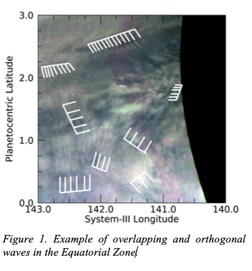
Long wave packets with short, dark wave fronts represent 79% of the types of waves in our inventory, especially in the Equatorial Zone (EZ) that were also detected in previous studies.  These include wave trains with orthogonal wave crests.  Even more commonly, we detected wave packets with tilted fronts that are not oriented orthogonally to the wave packet direction. Both the meridional extent and wavelength of these waves are much shorter than the Rossby deformation radius, so it is logical to assume that they are formed by and interact with small-scale turbulence, and thereby propagate the waves in all directions (Fig. 1). Sometimes the short wavefronts are aligned in curved wave packets, all associated with larger features, and located outside the EZ. 

Short wave packets with wide wave fronts were also detected.   In the Earth’s atmosphere, such waves are often associated with thunderstorms producing a brief impulse period with radiating waves.

Wave packets with bright features appear bright on a dark background rather than dark on a lighter background, like the waves described above.   Differences between darker and brighter wave crests could be the composition of the material affected.

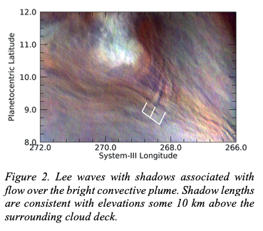
Lee waves, stationary waves generated by the vertical deflection of winds over an obstacle, were also detected. Jupiter’s atmosphere no doubt possesses the dynamical equivalent of an obstacle (Fig. 2).

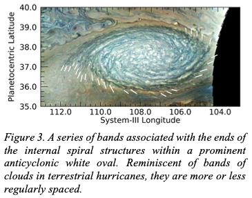
Waves associated with large vortices include compact cyclonic and anticyclonic features with extended radial wavefronts, resembling structures in terrestrial cyclonic hurricanes (Fig. 3). 

Long, parallel dark streaks are seen both with a non-uniform patterns and  in regularly spaced parallel bands.  Their orientation suggests that they are tracing out the direction of flow on streamlines.

Figure 4 plots the distribution of mean wavelengths for different types of waves and wave-like features as a function of latitude, co-plotted with mean zonal wind velocity.  The minimum distance between crests is 29.1 km. The variability of wavelengths within a single packet is typically no greater than 20-30%.  The equatorial waves with long packets and short crests in the EZ have wavelengths that are clustered between 30 km and 320 km, with most between 80 and 230 km in size.  No waves are found at latitudes associated with retrograde zonal flow unless associated with a larger atmospheric feature.

JunoCam, detected 157 waves or wave-like features in its first 20 perijove passes. Of these, 100 are waves with long, linear packets and short crests. Another 25were detected with short packets and long crests.  They are all likely to be truly propagating waves, which  form the vast majority of features detected, concentrated in a latitude range between 5ºS and 7ºN. Few of these appear to be associated with other features except for waves that appear to be oriented in lines of local flow. There were fewer waves in the EZ between the equator and 1ºN than there were immediately north and south of this band, which was different from the waves detected by Voyager imaging in 1979 that were more equally distributed.  Other waves outside the EZ are influenced by other features.  These include waves associated with an anticyclonic or cyclonic eddies, lee waves some 10 km above the surrounding cloud deck. Several features appeared within or emanating from vortices. Two sets of extremely long, curved features were detected near the edges of a southwestern extension of a region associated with high 5-µm radiances at the southern edge of the NEB.   No waves were detected south of 7ºS that were not associated with larger vortices, such as the GRS.  No waves or wave-like features were detected in regions of retrograde mean zonal flow that were not associated with larger features, similar to the waves detected by Voyager imaging.

Acknowledgements

The primary support for this research was provided by NASA, a portion of which was distributed to the Jet Propulsion Laboratory, California Institute of Technology. 

References

 [1] Hansen et al. Junocam: Juno’s outreach camera. Space Sci. Rev. 217, 475-506.  2017.

[2] Wong et al. High-resolution UV/optical/IR imaging of Jupiter in 2016–2019. Space Sci. Rev. 247, 58. 2020.

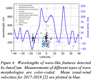
How to cite: Orton, G., Tabataba-Vakili, F., Rogers, J., and Hansen, C. and the JunoCam Waves Investigation Team: A Survey of Small-Scale Waves and Wave-Like Phenomena in Jupiter’s Atmosphere , Europlanet Science Congress 2020, online, 21 Sep–9 Oct 2020, EPSC2020-26, https://doi.org/10.5194/epsc2020-26, 2020.

Jupiter’s atmosphere displays some of the most dramatic weather of any planet in our Solar System, with cycles of activity changing the upper tropospheric and stratospheric temperatures, aerosols, and cloud structures through physical processes that are not yet well understood. In the troposphere, Jupiter’s banded structure undergoes dramatic planetary-scale disturbances that can evolve over short timescales changing its appearance completely at a range of altitudes, from the cloud tops (~500 mbar) to the deeper levels (1-4 bar). Some of these tropospheric variations seem to occur randomly, like the impressive fading and revival of the South Equatorial Belt at 7°-17° S (planetocentric latitude), while others follow a periodic pattern, like the North Equatorial Belt expansions at 7°-17° N (with a ~4.5-year periodicity), the Equatorial Zone disturbances (~7-year period) within ±7° of the equator (Antuñano et al. 2018 doi:  https://doi.org/10.1029/2018GL080382) and the convective outbreaks at 21° N in the North Temperate Belt (~5-year period) (Antuñano et al., 2019 doi: https://doi.org/10.3847/1538-3881/ab2cd6). In the stratosphere, Jupiter’s equatorial and off-equatorial temperature and winds at 10-20 mbar exhibit a remarkable 4-5-year periodic oscillation with height forced by waves produced from tropospheric meteorological activity at the equatorial latitudes.

Here we use almost 40 years (more than 3 jovian years) of ground-based infrared observations captured at NASA’s Infrared Telescope Facility (IRTF), the Very Large Telescope (VLT) and Subaru between 1980 and 2019 in a number of filters spanning from 7.9 to 24.5 µm.  These filters sample upper tropospheric and stratospheric temperatures and aerosols via collision-induced hydrogen and helium absorption, and emission from stratospheric hydrocarbons.  This long-term time series is used to (i) understand the impact of the previously mentioned tropospheric activity on the periodicity of the stratospheric temperature oscillations, (ii) characterize the long-term variability of Jupiter’s atmosphere at different altitudes in the upper troposphere and stratosphere, and (iii) investigate the long-term thermal, chemical and aerosol changes in Jupiter’s troposphere. In particular, we generate Lomb-Scargle periodograms and apply a Wavelet Transform analysis to our dataset to look for potential periodicities on the brightness temperature variability in different filters and compare them to previously reported cyclic activity at visible wavelengths (sensing the ammonia cloud top at ~500 mbar) and 5 µm (sensing the 1-4 bar pressure level). Finally, a Principal Component Analyses (PCA) is also performed to analyse the correlation of the brightness temperature variations at different belts and zones.

How to cite: Antunano, A., Fletcher, L. N., Orton, G. S., Sinclair, J. A., and Kasaba, Y.: Long-term Cycles of Variability of Jupiter’s Atmosphere from Ground-based Infrared Observations, Europlanet Science Congress 2020, online, 21 Sep–9 Oct 2020, EPSC2020-183, https://doi.org/10.5194/epsc2020-183, 2020.

Abstract

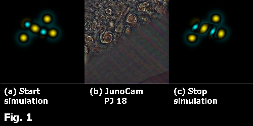
Comparing JunoCam images with simulation runs of two-dimensional Euler fluids reveals similarities between the morphology of Jupiter's cloud tops and simulated vorticity maps. We present examples of these analogies. They are required to establish conjectures that state these similarities in a more formal way.

Introduction and Context

JunoCam [1] has been collecting images of Jupiter's cloud tops for almost four years at the time of the submission of this abstract. In examining these images, we realized that two-dimensional simulations of Euler fluids [2] revealed patterns in vorticity fields reminiscent of structures in Jupiter's cloud tops. We pursue this initial observation further. A small collection of analogies between real data and simulations is presented, which inspire formal conjectures describing a correlation between vorticity and cloud features. These initial conjectures result in algorithm candidates that translate cloud morphology into vorticity and can be assessed and further refined on the basis of fluid-dynamical simulations.

In a larger-scale context, when two or more JunoCam images cover the same area of Jupiter with a time delay of several minutes, methods similar to stereo correspondence can be applied to retrieve velocity or vorticity field data. Displacements of corresponding areas of the surface between images can be used either to estimate a velocity field directly, or via the stream function component of a Helmholtz decomposition indirectly. Alternatively, measured rotations of surface areas can be used to estimate vorticities. Vorticity data inferred by any of these methods provide a low-resolution context and a reference for a refinement of the vorticity field on the basis of spatially higher-resolved morphological considerations.

The presentation will focus on a small survey of JunoCam images together with simulation runs developing structures similar to those observed in the images. This collection of examples is required for the empirical definition of formal conjectures connecting morphology with vorticity.

Example

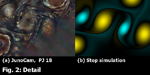
Figure 1 shows an excerpt of a map of Jupiter's north polar region during the PJ18 flyby that suggests a simplified model to initialize a simulation run. The initial model is simplified to consist of six Gauss vortices, representing four circumpolar cyclones (CPCs in yellow) and two anticyclonic white ovals (AWOs in blue). After a short simulation run, the vortices develop filamentary vorticity structures that are also apparent in the original JunoCam image, see detail in Fig. 2.

Conjectures

• The above example suggests that the brightness of the cloud tops is correlated with the total amount of the relative vorticity.

• Intact vortices of similar size that touch each other are of opposite sign. They form a filamentary structure between them consisting of two parallel filaments of opposite vorticity.

• Two nearby cyclones are separated by a filament of anticyclonic vorticity.

References

[1] C.J. Hansen, M.A. Caplinger, A. Ingersoll, M.A. Ravine, E. Jensen, S. Bolton, G. Orton. Junocam: Juno’s Outreach Camera. Space Sci Rev 2013:475-506, 2017

[2] G. Eichstädt, C. Hansen, G. Orton. Fluid Dynamical 2D Simulations of Jupiter's South Polar Region Based On JunoCam Image Data. EGU2020-12025,

How to cite: Eichstaedt, G., Hansen-Koharcheck, C., and Orton, G.: Comparing Selected JunoCam Images of Jupiter with Vorticity Fields Occuring In Simulations of Two-Dimensional Euler Fluids, Europlanet Science Congress 2020, online, 21 Sep–9 Oct 2020, EPSC2020-1007, https://doi.org/10.5194/epsc2020-1007, 2020.

Moist convective storms powered by the release of latent heat in rising air parcels are a key element of the meteorology of the Gas Giants [1] and are suspected to play also an important role in the atmospheric dynamics of the Ice Giants [2]. In Jupiter convective storms of different spatial scales occur with different frequencies, from short-lived localized storms [3] to longer-lived storms able to trigger planetary-scale disturbances that develop in cycles of several years [4].

Several models with different approaches have been developed to study moist convection in Jupiter and other planets [5-8]. Three-dimensional cloud resolving models are computationally expensive but have the advantage of allowing the study of the motions generated in the storm and they can also take into account the effects of the three-dimensional Coriolis force in the evolution of the storm. We have used an updated version of a three-dimensional Anelastic Model of Moist Convection [9-11] to explore the development of convective storms in Jupiter. We have improved the dynamical core of the model increasing the stability of the model, which allows us to simulate the dynamics of the development of the storms for longer time ranges than previous simulations presented with this model.

Here we will present results of new simulations of moist convective storms in Jupiter. We simulated the onset and initial development of the storms in a series of different scenarios of condensables abundances to study under which conditions it is possible to trigger convective storms. We tested different abundances of the condensables, relative humidities and fractions of condensates carried by the storm. We play particular attention to the capacity of the storm to generate convective downdrafts with the potential to desiccate the volatiles of the upper atmosphere [12, 13].

References:

[1] A. P. Ingersoll et al. Moist convection as an energy source for the large-scale motions in Jupiter’s atmosphere, Nature 403, 2000.

[2] R. Hueso and A. Sánchez-Lavega. Atmospheric Dynamics and Vertical Structure of Uranus and Neptune's weather layers, Space Science Reviews, 215:52, 2019.

[3] P. Iñurrigarro et al. Observations and numerical modelling of a convective disturbance in a large-scale cyclone in Jupiter’s South Temperate Belt, Icarus 336, 2020.

[4] A. Sánchez-Lavega et al. Depth of a strong jovian jet from a planetary-scale disturbance driven by storms, Nature 451, 2008.

[5] C. R. Stoker. Moist Convection: A Mechanism for Producing the Vertical Structure of the Jovian Equatorial Plumes, Icarus 67, 1985.

[6] Y. Yair et al. Model interpretation of Jovian lightning activity and the Galileo Probe results, Journal of Geophysical Research 103, 1998.

[7] K. Sugiyama et al. Numerical simulations of Jupiter’s moist convection layer: Structure and dynamics in statistically steady states, Icarus 229, 2014.

[8] C. Li and X. Chen. Simulating Nonhydrostatic Atmospheres on Planets (SNAP): Formulation, Validation and Application to the Jovian Atmosphere, The Astrophysical Supplement Series 240, 2019.

[9] R. Hueso and A. Sánchez-Lavega. A Three-Dimensional Model of Moist Convection for the Giant Planets: The Jupiter Case, Icarus 151, 2001.

[10] R. Hueso and A. Sánchez-Lavega. A three-dimensional model of moist convection for the giant planets II: Saturn’s water and ammonia moist convective storms, Icarus 172, 2004.

[11] R. Hueso and A. Sánchez-Lavega. Methane storms on Saturn’s moon Titan, Nature 442, 2006.

[12] T. Guillot et al. Storms and the Depletion of Ammonia in Jupiter: I. Microphysics of “Mushballs”, Journal of Geophysical Research, in press, 2020.

[13] T. Guillot et al. Storms and the Depletion of Ammonia in Jupiter: II. Explaining the Juno observations, Journal of Geophysical Research, in press, 2020.

How to cite: Iñurrigarro, P., Hueso, R., and Sánchez-Lavega, A.: Simulations of convective storms in Jupiter with an updated version of a three-dimensional model of moist convection, Europlanet Science Congress 2020, online, 21 Sep–9 Oct 2020, EPSC2020-284, https://doi.org/10.5194/epsc2020-284, 2020.

A fundamental challenge in the study of jovian atmospheres is the structure of the deep atmosphere, where the dynamics strongly influence the upper-troposphere. The clouds aloft obscure the deeper layers, making them difficult to observe without an atmospheric probe like Galileo. Nevertheless, the effect of the deep atmosphere is evident in the changes to the upper level clouds, either in short timescales, through the formation of convective plumes, or over long timescales in the case of planetary scale disturbances, which cause darkening/brightening of entire cloud bands (Fig 1). In the Pioneer and Voyager era, plumes of volatiles were observed to erupt from the deep atmosphere regularly, prompting the question of the strength of the internal heat flux within Jupiter’s atmosphere, and the role of moist convection in Gas Giant atmospheres. 

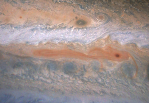
Fig 1: JunoCam image of the jet region where moist convective activity has led to planetary scale disturbances.

These plumes have been observed repeatedly near the eastward jet centered around 23.7° N latitude, in the between the North Tropical Belt and Zone. A set of plumes rise above the cloud deck and lead to the formation of a planetary-scale disturbance near the jet peak over several weeks (e.g., Sanchez-Lavega et al. 2008, 2017). Analysis of cloud formation on Jupiter considering the abundances of various condensible species revealed that the most likely source of these convective events was the deep water cloud which contains both the high density of volatiles and necessary convective potential to breach the upper cloud deck (Hueso et. al, 2002).

Preliminary modelling efforts of this region with the EPIC cloud scheme have yielded interesting results (Sankar et. al 2018, 2019). On perturbing the atmosphere, we noticed that rapid cloud formation was confined to narrow bands of latitude. To investigate this, we calculated the value of the Convective Available Potential Energy (CAPE) of water from the model output. We observed that the convective potential was stronger in regions within the jet and the North Equatorial Belt, which was primarily due to the strength of the jet affecting the thermal structure of the atmosphere. Cloud growth and formation of instabilities (seen as rapid cloud formation in the model) were stronger in regions of high CAPE, and cloud formation was supressed in regions of low CAPE (Fig 2). 

In this study, we use the Explicit Planetary Isentropic Coordinate (EPIC) atmospheric 3-dimensional general circulation model (GCM) to study the formation of Jovian moist convective events, using an active cloud microphysics scheme. We have updated this scheme using the Relaxed Arakawa-Schubert (RAS) moist convective scheme (Moorthi and Suarez, 1992) to parameterize sub-grid scale moist convective tendencies. The scheme diagnoses the changes in cloud mass and temperature due to the formation of several convective towers within a grid cell, which allows use to account for convective cumulus formation without having to directly resolving convective updrafts in our model. 

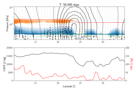
Fig 2: Meridional slice of simulation output showing cloud formation (top panel) and CAPE/CIN (bottom). Ammonia is orange-red and water is blue. The red line shows the level of neutral buoyancy and green line shows the level of free convection for a parcel starting at the base of the water cloud (~4 bars).

We focus on the region between 10° and 35° N, which encloses the jet at 23.7 N where plume formation has been observed several times. We initialize the atmosphere with different abundances of both water and ammonia, which are both treated as pure condensibles in our model, to understand the effect of deep abundance on the development of these convective outbursts. We will present our results from our test case before and after the addition of the moist convective scheme, and lessons learned from porting the scheme for use in gas giant atmsopheres.

How to cite: Sankar, R., Klare, C., and Palotai, C.: Moist convection in Jupiter's fastest jet, Europlanet Science Congress 2020, online, 21 Sep–9 Oct 2020, EPSC2020-469, https://doi.org/10.5194/epsc2020-469, 2020.

Microwave observations by the Juno spacecraft have shown that, contrary to expectations, the concentration of ammonia is still variable down to pressures of tens of bars in Jupiter. While mid-latitudes show a strong depletion, the equatorial zone of Jupiter has an abundance of ammonia that is high and nearly uniform with depth. In parallel, Juno determined that the Equatorial Zone is peculiar for its absence of lightning, which is otherwise prevalent most everywhere else on the planet. We show that a model accounting for the presence of small-scale convection and water storms originating in Jupiter’s deep atmosphere accounts for the observations. At mid-latitudes, where thunderstorms powered by water condensation are present, ice particles may be lofted high in the atmosphere, in particular into a region located at pressures between 1.1 and 1.5 bar and temperatures between 173K and 188K, where ammonia vapor can dissolve into water ice to form a low-temperature liquid phase containing about 1/3 ammonia and 2/3 water. We estimate that, following the process creating hailstorms on Earth, this liquid phase enhances the growth of hail-like particles that we call ‘mushballs’. Their growth and fall over many scale heights can effectively deplete ammonia, and consequently, water to great depths in Jupiter’s atmosphere. In the Equatorial Zone, the absence of thunderstorms shows that this process is not occurring, implying that small-scale convection can maintain a near homogeneity of this region. We predict that water, which sinks along with ammonia, should also be depleted down to pressures of tens of bars. Except during storms, Jupiter's deep atmosphere should be stabilized by the mean molecular weight gradient created by the increase in abundance of ammonia and water with depth.  This new vision of the mechanisms at play, which are both deep and latitude-dependent, has consequences for our understanding of Jupiter’s deep interior and of giant-planet atmospheres in general.

How to cite: Guillot, T., Stevenson, D. J., Bolton, S. J., Li, C., Atreya, S. K., Becker, H. N., Brown, S. T., Ingersoll, A. P., Janssen, M. A., Orton, G. S., Levin, S. M., Steffes, P. G., and Wong, M.: A depletion of ammonia and water by storms in the deep atmosphere of Jupiter, Europlanet Science Congress 2020, online, 21 Sep–9 Oct 2020, EPSC2020-512, https://doi.org/10.5194/epsc2020-512, 2020.

Introduction:  The locations of Jupiter’s cloud-top east-west jets are relatively constant over time and define the cyclonic belts and their neighbouring anticyclonic zones.  Thermal-infrared observations of the upper troposphere reveal cool temperatures, elevated abundances of condensate and disequilibrium gases, and enhanced cloud opacity over the zones, and the opposite over the belts (Gierasch et al., 1986, doi:10.1016/0019-1035(86)90125-9).  This distribution implies upwelling motions in zones and subsidence in belts. However, this picture has been called into question by the observed eddy-momentum flux convergence into the eastward jets (and divergence from the westward jets), which suggests a compensating flow in the opposite direction, from belts into zones, which is partially supported by the distribution of lightning at low latitudes (Little et al., 1999, doi:10.1006/icar.1999.6195).  It is possible that two different atmospheric regimes exist:  a deep regime where eddies are able to drive the zonal flows, and a higher-altitude regime where those zonal flows decay with height. Reconciling this apparent inconsistency remains a key challenge for the understanding of Jupiter’s atmosphere, and Juno observations of the deeper atmosphere shed important light on this issue. 

Methodology:  Juno’s Microwave Radiometer (MWR) examines the vertical structure of Jupiter’s belts and zones below the clouds by sounding in six channels from 1.4 to 50 cm, sensing from the cloud-tops at ~0.7 bar to pressures greater than 300 bar. Initial results (Li et al. 2017, doi:10.1002/2017GL073159) revealed contrasts at depth that bore a potential resemblance to the belt/zone structure in the upper troposphere.  We report on progress in our analysis of averaged nadir microwave brightness and its emission-angle dependence from the first two years of Juno’s mission.  We investigate the correlation between the meridional gradient of the brightness temperature at all emission angles and the cloud-top zonal winds.  These brightness temperature gradients reflect changes in gaseous opacity (e.g., ammonia and water), kinetic temperature, or both. We explore the implications of the contrasts observed between belts and zones as a function of depth sounded by MWR.

Preliminary Results:  Meridional brightness temperature gradients above the clouds (p<1 bar) were measured by the VLT/VISIR mid-infrared instrument in 2016, alongside the 1.37-cm MWR channel sensing temperatures and ammonia at p~0.7 bar. The gradients show a strong negative correlation with the cloud-tracked zonal winds and suggest a combination of zonal jet decay with altitude in the upper troposphere (e.g., Pirraglia et al., 1981, doi:10.1038/292677a0), along with depletion of volatiles (ammonia) within cyclonic belts.  MWR observations suggest that this negative correlation persists as deep as ~1.5 – 3.5 bar for both the tropical and temperate jets.  For the strong eastward jet near 6^oN, this is broadly consistent with results from both the Galileo Probe (Atkinson et al., 1998, doi:10.1029/98JE00060) and Cassini cloud-tracking (Li et al., 2006, doi:10.1029/2005JE002556), which suggested that the jet decayed with height from the ~5-bar level to the 0.5-bar level by more than 90 m/s.  We will report on our initial exploration of how these correlations change at deeper pressure levels by looking at MWR wavelengths beyond 10 cm, probing well below the expected condensation level of Jupiter’s water clouds.

Acknowledgements:  Fletcher was supported by a Royal Society Research Fellowship and European Research Council Consolidator Grant (under the European Union's Horizon 2020 research and innovation programme, grant agreement No 723890) at the University of Leicester.  Levin, Orton, and Oyafuso were supported by the National Aeronautics and Space Administration through funds distributed to the Jet Propulsion Laboratory, California Institute of Technology.

How to cite: Fletcher, L. N., Oyafuso, F., Allison, M., Ingersoll, A., Li, L., Kaspi, Y., Galanti, E., Wong, M., Orton, G., Zhang, Z., Li, C., Levin, S., and Bolton, S.: Jupiter's Temperate Belt/Zone Contrasts at Depth Revealed By Juno, Europlanet Science Congress 2020, online, 21 Sep–9 Oct 2020, EPSC2020-605, https://doi.org/10.5194/epsc2020-605, 2020.

Introduction

Previous studies of Jupiter’s wind patterns, from the Hubble Space Telescope and Cassini, revealed the southernmost two prograde jets at 58ºS and 64ºS (planetocentric), which we now designate as the S5 and S6 jets.  A few degrees further south they showed a retrograde flow, but the wind pattern further poleward was not well defined. It is important to characterise the flows in this region in order to understand the dynamics of the polar atmosphere and the processes that maintain the pentagon of cyclones around the south pole [1,2].  Here we use Juno (JunoCam) images to characterise the S5 and S6 jets and the wind patterns further south, up to the edge of the pentagon.

JunoCam takes hi-res images over the south polar region (SPR) at every perijove (PJ), which reveal the typical patterns of the region, in RGB and usually in the 0.89-µm CH₄ absorption band.  For each perijove we [G.E.] convert the RGB images into south polar projection maps, which can be ‘blinked’ or animated to visualise motions over ~0.5 to 2 hours.  They are also compiled into a composite map of most of the SPR. We use maps that go down to 60ºS at the edges (and further at the corners so part of the S5 jet is included).

Organisation of the SPR  [e.g. Fig.1]

Here we summarise general conclusions from JunoCam at all perijoves up to PJ23, from alignments of the RGB maps, the wind motions in animations, and the CH₄ maps.

The S5 jet is narrow and coincides exactly with a slightly sinuous boundary in methane images, the band to the south being methane-dark.  The S6 jet is faster, broader and highly undulating in latitude.  It generally coincides with the sinuous edge of the methane-bright South Polar Hood (SPH).   In CH₄ maps the wave pattern previously recorded [3] is always present around most or all of the circumference, with greater or lesser regularity.  Often the pattern is regular with wavelengths of 20-36º longitude (the mean from 8 perijoves is 25.5º ±2.6º) and amplitudes up to 3º latitude peak-to-trough. 

The SPR in RGB is dark, with an irregular edge that lies between the S5 and S6 jets.  It appears relatively bluer south of the S6 jet, apparently because SPH overlying it is a relatively bluish haze.

Poleward of the S6 jet, there is an irregular cyclonic belt of folded filamentary regions (FFRs) at ~65-70ºS.  They show typically rapid circulation and the retrograde part of this along their south edges could be regarded as a retrograde jet at ~71ºS; however this is only present within the FFRs, not between them.  Several AWOs are usually present close to the south edge of this belt of FFRs.

Further south, where the dominant features are scattered irregular FFRs and a few anticyclonic white ovals (AWOs), there are no permanent nor rapid nor extended jets.  There are sometimes short, weak prograde flows in mid-latitudes, ~74-77ºS, a few tens of degrees long. Some of these appear to be merely the flanks of flows within FFRs just to the south; others are oblique. There is no jet around the south polar pentagon.

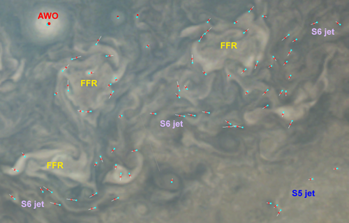
Wind-speed measurements  [e.g. Fig.2]

For each of PJ15, PJ16, and PJ17, a pair of single-image maps was aligned and blinked, and hundreds of points were marked on each map manually for feature tracking. Points were chosen on and near the most rapid currents, i.e. the peaks of the S5 and S6 jets and the outer parts of FFRs, so as to define these flows. 

We find that the S6 jet is rapid at all longitudes, and of variable width.  It traces large waves in latitude, generally coinciding with the wave pattern around the edge of the methane-bright SPH, though with a few local exceptions.  Mean peak wind speeds (measured along the jet rather than strictly eastward) range from 42 (±12) to 49 (±11) m/s. These are higher than previous speeds from Cassini and HST (25 to 42 m/s), probably because those were zonal averages diminished by the sinuosity of the jet.  This sinuosity of the S6 jet (and more weakly, the S5 jet) contrasts with the straight flow of all lower-latitude prograde jets.

Wind speeds were also measured in FFRs in the main belt and further south.  They were generally in the range of ~20-60 m/s, without obvious dependence on wind direction or latitude.  Mean speeds in each FFR ranged from 31 to 43 m/s, averaging 37 (±13) m/s.  (However, more diverse speeds may exist in some unmeasured FFRs.)  These speeds are comparable to those measured in other cyclonic structures at lower latitudes.

Conclusions

The S6 jet is highly sinuous, coinciding with the prominent waves around the edge of the methane-bright SPH.  There are no prograde jets closer to the pole. A belt of FFRs immediately south of the S6 jet includes fast retrograde speeds around ~71ºS.

The JunoCam maps alone cannot trace slower motions of larger features, notably FFRs, but this can be partially achieved with inclusion of ground-based maps: see our companion abstract in session ODAA3 [4].

References

Fig.1.  Polar projection map from PJ20.  Yellow circles mark the circumpolar cyclones. Inset:  CH₄ map at reduced scale. 

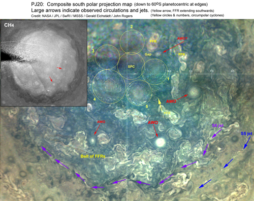
Fig.2.  Excerpt from a map at PJ16 with points measured for feature tracking indicated.

How to cite: Rogers, J., Eichstädt, G., Hansen, C., Orton, G., and Momary, T.: Jupiter’s south polar region (~60-80ºS): Wind patterns from JunoCam maps, Europlanet Science Congress 2020, online, 21 Sep–9 Oct 2020, EPSC2020-151, https://doi.org/10.5194/epsc2020-151, 2020.

We present results of simulations of the growth of giant planets that incorporate the mixing of light gases with denser material that enters the planet as solids. We find that heavy compounds and gas begin to intimately mix when the planet is quite small, and substantial mixing occurs when the planet becomes roughly as massive as Earth, because even incoming silicates can then fully vaporize if they arrive in the form of planetesimals or smaller bodies. Nonetheless, most of the icy and rocky material accreted by a giant planet settles to a region in which vaporized ice and rock are well-mixed until the growing planet is several times as massive as Earth. Subsequently, planetesimals break up in a region that is too cool for all the silicates to vaporize, so the silicates continue to sink, but the water remains at higher altitudes. As the planet continues to grow, silicates vaporize farther out. Because the mean molecular weight decreases rapidly outward at many radii, some of the radially inhomogeneities in composition produced during the accretion era are able to survive for billions of years. After 4.57 Gyr, our model Jupiter retains compositional gradients; from the inside outwards one finds: (i) an inner core, dominantly composed of heavy elements; (ii) a density-gradient region, containing the majority of the planet's heavy elements, where H and He increase in abundance with height, reaching ~90% mass fraction at 30% of Jupiter's radius, with rocky materials enhanced relative to ices in the lower part of this gradient region and the composition transitioning to ices enhanced relative to rock at higher altitudes; (iv) a large, uniform-composition region (we do not account for He immiscibility), enriched relative to protosolar in heavy elements, especially ices, that contains the bulk of the planet's mass; and (v) an outer region where condensation of many constituents occurs. This radial compositional profile has heavy elements more broadly distributed within the planet than predicted by classical Jupiter-formation models. NASA’s Juno spacecraft's measurements of Jupiter's gravity field also implies less concentration of heavy elements near the center of the planet than classical theoretical models. However, the preferred dilution of the core found in Juno-constrained gravity models is substantially larger than what is suggested by our accretion models, requiring some modification in the heavy element distribution. The compositional gradients in the region containing the bulk of the planet’s heavy elements prevent convection, both in our models and the models that fit current gravity, probably resulting in a hot deep interior where much of the energy from the early stages of the planet's accretion remains trapped.

How to cite: Lissauer, J., Bodenheimer, P., Stevenson, D., and D'Angelo, G.: Mixing of Condensable Constituents with H/He During Formation of the Jupiter , Europlanet Science Congress 2020, online, 21 Sep–9 Oct 2020, EPSC2020-145, https://doi.org/10.5194/epsc2020-145, 2020.

How to cite: Duer, K., Galanti, E., and Kaspi, Y.: The statistical probability of deep flow structures that fit Jupiter's asymmetric gravity , Europlanet Science Congress 2020, online, 21 Sep–9 Oct 2020, EPSC2020-182, https://doi.org/10.5194/epsc2020-182, 2020.

Juno's observations of Jupiter's gravity field have revealed extremely low values for the gravitational moments that are difficult to reconcile with the high abundance of metals observed in the atmosphere by Galileo. Recent studies chose to arbitrarily get rid of one of these two constraints in order to build models of Jupiter.

In this presentation, I will detail our new Jupiter structure models reconciling Juno and Galileo observational constraints. These models confirm the need to separate Jupiter into at least 4 layers: an outer convective shell, a non-convective zone of compositional change, an inner convective shell and a diluted core representing about 60 percent of the planet in radius. Compared to other studies, these models propose a new idea with important consequences: a decrease in the quantity of metals between the outer and inner convective shells. This would imply that the atmospheric composition is not representative of the internal composition of the planet, contrary to what is regularly admitted, and would strongly impact the Jupiter formation scenarios (localization, migration, accretion).

In particular, the presence of an internal non-convective zone prevents mixing between the two convective envelopes. I will detail the physical processes of this semi-convective zone (layered convection or H-He immiscibility) and explain how they may persist during the evolution of the planet.

These models also impose a limit mass on the compact core, which cannot be heavier than 5 Earth masses. Such a mass, lower than the runaway gas accretion minimum mass, needs to be explained in the light of our understanding of the formation and evolution of giant planets.

Using these models of Jupiter, I will finally detail the application of our new understanding of the interior of this planet to giant exoplanets. At a time of direct imaging of extrasolar planets and atmospheric characterization of hot Jupiters, a good understanding of the internal processes of planets in the solar system is paramount to make the best use of all the observations.

How to cite: Debras, F. and Chabrier, G.: New models of Jupiter in the context of Juno and Galileo: signature of a decoupling between the atmosphere and the interior, Europlanet Science Congress 2020, online, 21 Sep–9 Oct 2020, EPSC2020-681, https://doi.org/10.5194/epsc2020-681, 2020.

The strong zonal flows observed at the cloud-level of the gas giants extend thousands of kilometers deep into the planetary interior, as indicated by the Juno and Cassini gravity measurements. However, the gravity measurements alone, which are by definition an integrative measure of mass, cannot constrain with high certainty the detailed vertical structure of the flow below the cloud-level. Here we show that taking into account the recent magnetic field measurements of Saturn and past secular variations of Jupiter's magnetic field, give an additional physical constraint on the vertical decay profile of the observed zonal flows in these planets. In Saturn, we find that the cloud-level winds extend into the planet with very little decay (barotropically) down to a depth of around 7,000 km, and then decay rapidly, so that within the next 1,000 km their value reduces to about 1% of that at the cloud-level. This optimal deep flow profile structure of Saturn matches simultaneously both the gravity field and the high-order latitudinal variations in the magnetic field discovered by the recent measurements. In the Jupiter case, using the recent findings indicating the flows in the planet semiconducting region are order centimeters per second, we show that with such a constraint, a flow structure similar to the Saturnian one is consistent with the Juno gravity measurements. Here the winds extend unaltered from the cloud-level to a depth of around 2,000 km and then decay rapidly within the next 600 km to values of around 1%. Thus, in both giant planets, we find that the observed winds  extend unaltered (baroctropically) down to the semiconducting region, and then decay abruptly. While it is plausible that the interaction with the magnetic field in the semiconducting region is responsible for winds final decay, it is yet to be understood whether another mechanism is involved in the process, especially in the initial decay form the strong 10s meter per seconds winds.

How to cite: Galanti, E. and Kaspi, Y.: Synergized magnetic and gravity measurements probe the detailed structure of the gas giants' deep atmospheres, Europlanet Science Congress 2020, online, 21 Sep–9 Oct 2020, EPSC2020-84, https://doi.org/10.5194/epsc2020-84, 2020.

The nature and structure of the observed east-west flows on Jupiter and Saturn has been a long-standing mystery in planetary science. This mystery has been recently unraveled by the accurate gravity measurements provided by the Juno mission to Jupiter and the Grand Finale of the Cassini mission to Saturn. These two experiments, which coincidentally happened around the same time, allowed the determination of the overall vertical and meridional profiles of the zonal flows on both planets. In this talk, we discuss what has been learned about the zonal jets on the gas giants in light of the new data from these two experiments. The gravity measurements not only allow the depth of the jets to be constrained, yielding the inference that the jets extend to roughly 3000 and 9000 km below the observed clouds on Jupiter and Saturn, respectively, but also provide insights into the mechanisms controlling these zonal flows. Specifically, for both planets this depth corresponds to the depth where electrical conductivity is within an order of magnitude of 1 S/m, implying that the magnetic field likely plays a key role in damping the zonal flows. An intrinsic characteristic of any gravity inversion, as discussed here, is that the solutions might not be unique. We analyze the robustness of the solutions and present several independent lines of evidence supporting the inference that the jets reach these depths.

How to cite: Kaspi, Y., Galanti, E., Showman, A., Stevenson, D., Guillot, T., Iess, L., and Bolton, S.: Comparison of the deep atmospheric dynamics of Jupiter and Saturn in light of the Juno and Cassini gravity measurements, Europlanet Science Congress 2020, online, 21 Sep–9 Oct 2020, EPSC2020-345, https://doi.org/10.5194/epsc2020-345, 2020.

Although studied for many years, the powerful ultraviolet auroral emissions at Jupiter still contain many mysteries. Even well-established theories explaining the Jovian main auroras are now questioned in the light of observations by the Juno spacecraft currently orbiting the giant planet. Jupiter’s aurora is known to respond to changes in solar wind on one hand and to processes occurring inside the magnetosphere on the other hand. However, many changes regularly observed in the aurora could not yet be categorized as solar wind-driven or as internally-driven dynamics. An observing campaign of the Jovian aurora with the Hubble Space Telescope (HST) has been performed between February and September 2019 (HST GO-15638), including approximately 10 visits around each of the perijoves of Juno’s orbits 18 to 22. During this time, the solar activity was minimal, giving the opportunity to investigate auroral dynamics mainly controlled by internal processes. The main emission often appeared dim and diffuse (see the example on Figure 1), in particular on the dawn side where a narrow arc is generally found. In contrast, emissions poleward of the main emission were very dynamic, exhibiting some periodic brightening and intensities occasionally increasing tenfold over a few minutes (like in the middle panel of Figure 1). Many other interesting features are observed, such as dawn storms, duplication of the main emission, fresh and old injection signatures and transpolar arcs. All of these emissions are investigated by combining HST high temporal and spatial resolution images with in situ data simultaneously collected by Juno in Jupiter’s magnetosphere. Additionally, some HST visits have been scheduled while Juno-UV Spectrograph was observing the opposite hemisphere at the same time, enabling the tracking of conjugate auroral features in both hemispheres simultaneously.

Figure 1: Sequence of polar projections of HST images of the northern aurora at Jupiter, taken on September 10, 2019.

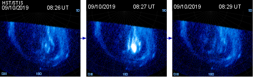
How to cite: Palmaerts, B., Grodent, D., Bonfond, B., Yao, Z., Guo, R., Dumont, M., Gérard, J.-C., and Haewsantati, K.: Jupiter's aurora liveliness during solar minimum, Europlanet Science Congress 2020, online, 21 Sep–9 Oct 2020, EPSC2020-1000, https://doi.org/10.5194/epsc2020-1000, 2020.

In July of 2016, NASA began a new era in Jupiter exploration by placing the Juno spacecraft and its highly capable suite of scientific instrumentation in a polar orbit about Jupiter. It was a unique opportunity to study Jupiter’s auroras in great details with the Ultraviolet Spectrograph (UVS) instrument during the first 25 perijoves. Here we present a systematic analysis of a newly identified feature of the polar emissions called the auroral bright spot. The bright spots have power ranging from tens to a hundred gigawatts. In a given perijove, bright spot reoccurs at almost the same system III (SIII) position within a time interval of a few to tens of minutes. Furthermore, we found a brightness quasiperiodicity of 22-28 minutes in the southern bright spots observed during perijove 4 and perijove 16. The northern bright spots locate in a confined region, near 175° SIII longitude and 65 degrees latitude, while the southern spots scatter randomly around the pole. The bright spots’ positions reported here are usually located on the edge of the swirl region (the polar-most region of Jupiter’s auroras). This feature is observed at all magnetic local times rather than being confined to the noon sector. Therefore, the bright spot is incompatible with the auroral signature of Earth-like Sun-facing cusp, as proposed in earlier works. However, due to Jupiter's rapid rotation with respect to the size of the magnetosphere, the topology of the cusp region at Jupiter is expected to be considerably complicated by the twisting of the field lines. Hence, we cannot conclude whether the bright spot is related to the Jovian cusp processes yet. Finally, we also have identified time intervals during which Juno flew through the field lines connected to the bright spot allowing further investigations of the associated particles and responsible processes.

How to cite: Haewsantati, K., Bonfond, B., Wannawichian, S., Gladstone, G. R., Hue, V., Versteeg, M. H., Greathouse, T. K., Grodent, D., Yao, Z., Dunn, W., Gérard, J.-C., Giles, R. S., Kammer, J. A., Guo, R., and Vogt, M. F.: Bright spot auroras in Jupiter’s polar region: Juno-UVS observations, Europlanet Science Congress 2020, online, 21 Sep–9 Oct 2020, EPSC2020-104, https://doi.org/10.5194/epsc2020-104, 2020.

Ionospheric conductance is important in controlling the electrical coupling between the Jovian planetary magnetosphere and its ionosphere. To some extent, it regulates the characteristics of the ionospheric current from above and the closure of the magnetosphere-ionosphere circuit in the ionosphere (Cowley&Bunce, 2001). Multi-spectral images collected with the UltraViolet Spectrograph (UVS) (Gladstone et al., 2017) on board Juno (Bagenal et al.,2017) have been analyzed to derive the spatial distribution of the auroral precipitation reaching the atmosphere (Bonfond et al., 2017). Electron energy flux and their characteristic energy have been used as inputs to an ionospheric model providing the production and loss rates of the main ion species, H₃⁺, hydrocarbon ions and electrons (Gérard et al., 2020). Their steady state densities are calculated and used to determine the local distribution of the Pedersen electrical conductivity and its altitude integrated value for each UVS pixel. These values are displayed as H₃⁺ density and Pedersen conductivity maps. We find that the main contribution to the Pedersen conductance corresponds to collisions of H₃⁺ and hydrocarbon ions with H₂.

Analysis of the Birkeland current intensities based on the Juno magnetometers measurements (Kotsiaros et al. 2019) indicated that the observed current intensities are statistically larger in the south. They suggested that these differences are possibly due to a higher Pedersen conductance in this hemisphere. In order to verify this hypothesis, we calculate the conductance and H₃⁺ density maps for perijoves 1 to 15 based on Juno-UVS spectral images. We compare the spatially integrated auroral conductance values of the two hemispheres for each orbit.  The objective is to identify possible hemispheric asymmetries.   

REFERENCES

Bagenal, F., et al. (2017). Magnetospheric science objectives of the Juno mission. Space Science Reviews, 213(1-4), 219-287.

Bonfond, B., et al. (2017). Morphology of the UV aurorae Jupiter during Juno's first perijove observations. Geophysical Research Letters, 44(10), 4463-4471.

Cowley, S.W.H. & Bunce, E.J. (2001). Origin of the main auroral oval in Jupiter’s coupled magnetosphere–ionosphere system. Planet. Space Sci. 49, 1067–1088.

Gérard et al., Spatial distribution of the Pedersen conductance in the Jovian aurora from Juno-UVS spectral images, J. Geophys. Res., in press.

Gladstone et al. (2017). The ultraviolet spectrograph on NASA’s Juno mission. Space Science Reviews, 213(1-4), 447-473.

Kotsiaros, S. et al. (2019). Birkeland currents in Jupiter’s magnetosphere observed by the polar-orbiting Juno spacecraft. Nature Astronomy, 3(10), 904-909.

How to cite: Gérard, J.-C., Gkouvelis, L., Bonfond, B., Gladstone, R., Blanc, M., Grodent, D., Hue, V., Greathouse, T., Kammer, J., and Verteeg, M.: Jovian auroral conductance from Juno-UVS: hemispheric asymmetry?, Europlanet Science Congress 2020, online, 21 Sep–9 Oct 2020, EPSC2020-325, https://doi.org/10.5194/epsc2020-325, 2020.

The Main Emissions are the most recognizable feature of the aurorae at Jupiter and they are responsible for roughly 1/3rd of the total emitted power. They form an ever-present and quasi-continuous ring of emission centered on the magnetic poles. The most widely accepted explanation for these auroral emissions involves a current system related to the corotation enforcement of the plasma in the Jovian magnetosphere. Models based on this theory explain many characteristics of the aurorae. However, recent observations from the NASA Juno spacecraft and the ESA/NASA Hubble Space Telescope, complemented by previous results from the NASA Galileo spacecraft, challenge this theoretical framework. In this presentation, we will review six specific sets of observations contradictory with expectations from the corotation enforcement theory:

We will expose their implications for the modelling of the Jovian magnetosphere and aurorae and we will discuss promising paths forward. 

How to cite: Bonfond, B., Yao, Z., and Grodent, D.: Six observational pieces of evidence against corotation as the main cause for the aurora at Jupiter , Europlanet Science Congress 2020, online, 21 Sep–9 Oct 2020, EPSC2020-29, https://doi.org/10.5194/epsc2020-29, 2020.

Abstract

We present an extensive statistical study of all 29 Chandra High Resolution Camera (HRC-I) observations, covering ∼ 20 years worth of data from 18th December 2000 to 8th September 2019. Eight of these observations were pre-Juno and 21 while Juno was exploring the Jovian system providing in situ context. The first spatially resolved X-ray auroral "hot spot" was discovered by Gladstone et al. (2002) from Chandra observations of Jupiter’s North Pole. The emissions observed were found to pulsate with a 45-min quasi-periodic oscillation (QPO) and believed to originate in the outer magnetosphere (> 30 RJ) [1]. Since then, from using subsequent remote sensing X-ray observations in tandem with available in situ data, we know that the emissions from the hot spot consist of soft X-rays (SXRs, photons with energy < 2 keV) from charge exchange processes between precipitating ions and neutrals within the Jovian atmosphere [2]. However, the hot spot is found to be very variable both spatially and temporally [3] in all observations to date, thus proving determining the driver to be very difficult.

In this study, we characterise the typical and extreme behaviour of the hot spot emissions across the entire catalogue for the first time. Examining both types of behaviour allows us to determine the full extent of hot spot variability. We mainly focus on the northern hot spot (NHS) as: (1) the viewing geometry over the catalogue favours the North Pole best and (2) the NHS has been shown to be mostly non-conjugate with the south [4, 5], producing much stronger emission. We present heat maps and 2-D histograms to show the overall average hot spot morphology. The hot spot was defined using a numerical criterion of location and photon concentration (S3 longitude: 100° - 240°; latitude: 40° - 90°; concentration: > 7 photons per 5° S3 lon × 5° lat) [6]. From the catalogue, 26 out of 29 observations had emission within this threshold. Using a 2-D histogram with 3° S3 lon × 3° lat binning, we find a significant region of concentrated NHS emission at ∼ 162° - 171° S3 longitude and 60° - 66° latitude, herein referred to as the averaged hot spot nucleus (AHSNuc). The AHSNuc is found to mainly map to the noon magnetopause boundary while most events from the NHS are found to originate on the dusk-midnight boundary. This suggests that multiple drivers may produce the NHS. The mapping is carried out using a flux equivalence model [7, 8] with the Grodent Anomaly Model (GAM) [9], to model the internal field. We discuss the uncertainty in our mapping associated with possible fluctuations in ionospheric position and mapping limitations to improve the accuracy of our interpretations.

Finally, we apply the Rayleigh test technique discussed in Jackman et al. (2018) to find any significant QPOs within the hot spot and the AHSNuc.
We create a catalogue of all our timing analysis results noting all the significant QPOs found and test their robustness using a Jackknife test. We interpret the NHS and AHSNuc locations and compare the timescales of the QPOs to known possible drivers (such as magnetopause reconnection [10] and ultralow frequency (ULF) waves [11]) in an attempt to determine the overall hot spot driver/drivers.

References
[1] Gladstone, R.G.; Waite, J.; Grodent, D. et al.: A pulsating auroral X-ray hot spot on Jupiter, Nature, Vol. 415, pp. 1000-1002, 2002.

[2] Branduardi-Raymont, G., Elsner, R. F., Galand, M. et al.: Spectral morphology of the X-ray emission from Jupiter’s aurorae, Journal of Geophysical Research: Space Physics, Vol. 113, pp. 1-11, 2008.

[3] Jackman, C. M., Knigge, C., Altamirano, D. et al.: Assessing Quasi-Periodicities in Jovian X-Ray Emissions: Techniques and Heritage Survey, Journal of Geophysical Research: Space Physics, Vol. 123, pp. 9204-9221, 2018.

[4] Dunn,W. R., Branduardi-Raymont, G., Ray, L. C. et al.: The independent pulsations of Jupiter’s northern and southern X-ray auroras, Nature Astronomy, Vol. 1, pp 758-764, 2017.

[5] Wibisono A. D., Branduardi-Raymont, G., Dunn, W. R. et al.: Temporal and Spectral Studies by XMM-Newton of Jupiter's X-ray Auroras During a Compression Event, Journal of Geophysical Research: Space Physics, Vol. 125, e2019JA027676, 2020.

[6] Weigt, D. M., Jackman, C. M., Dunn, W. R. et al.: Chandra Observations of Jupiter’s X-ray Auroral Emission During Juno Apojove 2017, Journal of Geophysical Research: Planets, Vol. 125, e2019JE006262, 2020.

[7] Vogt, M. F., Kivelson, M. G., Khurana, K. K. et al.: Improved mapping of Jupiter’s auroral features to magnetospheric sources, Journal of Geophysical Research: Space Physics, Vol. 116, A03220, 2011.

[8] Vogt, M. F., Bunce, E. J., Kivelson, M. G. et al.: Magnetosphere-ionosphere mapping at Jupiter: Quantifying the effects of using different internal
field models, Journal of Geophysical Research: Space Physics, Vol. 120, pp. 2584–2599, 2015.

[9] Grodent, D., Bonfond, B., Gérard, J. C. et al.: Auroral evidence of a localized magnetic anomaly in Jupiter’s northern hemisphere, Journal of Geophysical Research: Space Physics, Vol. 113, pp. 1-10, 2008.

[10] Ebert, R.W., Allegrini, F., Bagenal, F. et al.: Accelerated flows at Jupiter’s magnetopause: Evidence for magnetic reconnection along the dawn flank. Geophysical Research Letters, Vol. 44, pp. 4401–4409, 2017.

[11] Manners, H., Masters, A., and Yates, J.N.: Standing Alfvén waves in Jupiter’s magnetosphere as a source of ∼ 10- to 60-min quasiperiodic pulsations, Geophysical Research Letters, Vol. 45, pp. 8746–8754, 2018.

How to cite: Weigt, D., Jackman, C., Vogt, M., Manners, H., Dunn, W., Gladstone, R., Kraft, R., and Branduardi-Raymont, G.: Characteristics of Jupiter's X-ray auroral hot spot emissions using Chandra, Europlanet Science Congress 2020, online, 21 Sep–9 Oct 2020, EPSC2020-357, https://doi.org/10.5194/epsc2020-357, 2020.

Ionospheric outflow is the outward flow of atmospheric plasma, initiated by a loss of equilibrium along the magnetic field. Terrestrial ionospheric outflow presents as a polar wind triggered by the Dungey cycle, which drives much of Earth’s magnetospheric dynamics. At Saturn, Felici et al. [2016] observed ionospheric outflow in the lobes at 36 R_S. Interestingly, at Jupiter, Valek et al. [2019] reported ionospheric outflow on magnetic field lines with invariant latitudes between Io’s auroral signatures and the main auroral emission, lower than the polar cap.

At Jupiter and Saturn, the rapid rotation of the planet, coupled with an internal plasma source inside each magnetosphere, results in the Vasyliunas cycle, by which material is circulated throughout the system, eventually being lost down the magnetotail. This constant churning likely results in a system where ionospheric outflow occurs more readily at mid-to-high planetary latitudes that map to the middle magnetosphere, rather than solely at polar latitudes. Furthermore, ionospheric outflow at the Jupiter and Saturn will be affected by strong centrifugal forces and auroral currents, which are near omnipresent in each magnetosphere.

Using a 1-dimensional, hydrodynamic, multi-fluid model, we determine the ionospheric outflow in the jovian and saturnian systems. Our model includes the effect of centrifugal forces and auroral field-aligned currents, both of which act to enhance outflow rates from previous studies. We find that ionospheric outflow may provide a significant contribution to the jovian and saturnian systems, with the mass source rates of 18.7 – 31.7 kg s^-1and 5.5-17.7 kg s^-1, respectively, where the range reflects the sensitivity to the assumed initial atmospheric conditions.

How to cite: Martin, C., Ray, L., Constable, D., Southwood, D., Felici, M., Lorch, C., Kinrade, J., and Gray, R.: Ionospheric Outflow at Jupiter and Saturn, Europlanet Science Congress 2020, online, 21 Sep–9 Oct 2020, EPSC2020-369, https://doi.org/10.5194/epsc2020-369, 2020.

We combine RPWS/LP and INMS data from Cassini's Grand Finale orbits into Saturn's lower ionosphere to calculate the effective recombination coefficient α₃₀₀ at a reference electron temperature of 300 K. Assuming photochemical equilibrium at altitudes below 2500 km and using an established method to determine the electron production rate, we derive upper limits for α₃₀₀ of ∼ 2.5∗10^-7 cm³ s^-1, which suggest that Saturn's ionospheric positive ions are dominated by species with low recombination rate coefficients.
An ionosphere dominated by water group ions or complex hydrocarbons, as previously suggested, is incompatible with this result, as these species have recombination rate coefficients > 5∗10^-7 cm³ s^-1 at an electron temperature of 300 K. The results do not give constraints on the nature of the negative ions.

How to cite: Dreyer, J., Vigren, E., Morooka, M., Wahlund, J.-E., Buchert, S., and Waite, J. H.: Using the effective recombination coefficient to constrain the positive ion composition in Saturn's ionosphere, Europlanet Science Congress 2020, online, 21 Sep–9 Oct 2020, EPSC2020-451, https://doi.org/10.5194/epsc2020-451, 2020.

Jupiter’s UV and X-ray aurorae were first discovered in 1979 by Voyager 1 and the Einstein Observatory, respectively. The auroral morphology comprises an oval ring of UV and high energy, or “hard”, X-rays and both emissions are produced by the same population of energetic electrons (Branduardi-Raymont et al., 2008). As the electrons precipitate into the gas giant’s atmosphere, they can excite molecular and atomic hydrogen that will then release UV photons while returning back to the ground state. The electrons can also emit bremsstrahlung radiation in the X-ray waveband as they are slowed and deflected by the molecules in the atmosphere. Within this oval is a second source of X-ray emissions with lower energies, as well as diffuse UV emissions. These “soft” X-rays are the result of ions charge exchanging with neutrals in Jupiter’s atmosphere. Observational and theoretical studies seem to favour an iogenic origin for these ions (e.g. Wibisono et al., 2020; Cravens et al., 1995), however, there are instances where the spectrum is better fit by the inclusion of solar wind ions (Dunn et al., 2020). The ion emissions also often pulse with periods of tens of minutes (e.g. Gladstone et al., 2002; Jackman et al., 2018).

The aurora in both wavebands is responsive to changing conditions inside and outside of Jupiter’s magnetosphere (Grodent et al., 2018). For example, the dawnside main emission of the UV aurora is dim and thin when the magnetosphere is undisturbed and contains very little plasma. The appearance of dawn storms, or short-lived brightenings in the dawnside main oval emission, is associated with tail reconnection events (Yao et al., in review) and is usually accompanied by a distinct enhancement equatorward of the main emission towards the dusk sector. This feature is caused by strong injections of magnetospheric plasma (Mauk et al. 2002). A solar wind compression results in a very bright and defined main oval in the dawn sector and bright poleward emissions in the dusk sector. Previous studies have shown that the X-ray aurora brightens during solar wind compressions but it can also do so during intervals of quiet solar wind, possibly suggesting control by sources internal to the magnetosphere (Dunn et al., 2020). However, signatures in the X-rays that point to mass loading and injection events having happened have not yet been identified.

Juno’s 22^nd perijove on 12 September 2019 was supported by remote observations of Jupiter from XMM-Newton, Chandra, the Hubble Space Telescope and Hisaki. XMM-Newton undertook an unprecedented 405 ks-long campaign between 8 and 14 September 2019 and recorded the X-ray aurora changing its behaviour throughout this time (see Figures 1-3). The spacecraft made 3 orbits around the Earth during this time hence why there are 3 sets of spectra and lightcurves and the gaps in the lightcurves are due to XMM-Newton perigee passages. Images of the UV aurora from Hubble show dawn storms and injection events at least twice during those six days. Hisaki data also show that the Io Plasma Torus and EUV aurora were responding to internally driven processes around this time. Juno’s location at local midnight allowed it the perfect opportunity to confirm whether tail reconnection had happened and detect plasmoids that may have been shot back towards Jupiter. We present our findings of how these mass loading and magnetospheric plasma injection events leave their marks on the timing and spectral properties of the X-ray aurora.

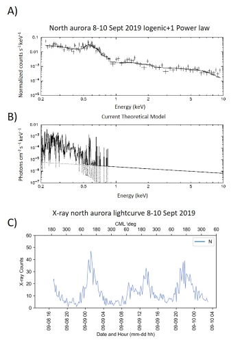
Figure 1: XMM-Newton EPIC-pn spectra (crosses on panel A) and EPIC light travel time shifted lightcurves (panel C) of Jupiter’s X-ray aurora from 8-10 September 2019. The spectrum is best fitted with an atomic charge exchange model for an iogenic (sulphur and oxygen) plasma population and a power law continuum. Panel B shows the theoretical spectra of the models used which were then convolved with the instrument response to give the black lines that are plotted over the data in panel A. The aurora is very bright during the first XMM-Newton orbit with a high flux above 1 keV in the spectrum and the corresponding lightcurve shows some regular pulsations.

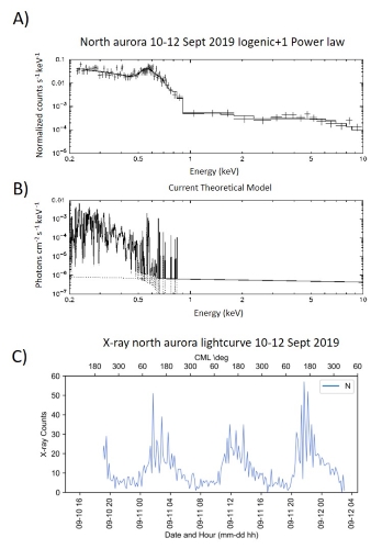
Figure 2: Same format as Figure 1 but for 10-12 September 2019. There is an increased amount of soft X-ray emissions in the second orbit with very dim hard X-ray emissions. Bright flares were emitted at ~02:00 and ~22:00 UT on 11 September and strong quasi-periodic pulsations in the aurora occurred during much of this orbit.

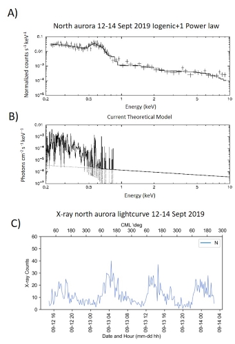
Figure 3: Same format as Figure 1 but for 12-14 September 2019. The spectrum for the final orbit now illustrates a decreased amount of soft X-ray emissions and brightened hard X-ray emissions; the lightcurve shows that the aurora had stopped pulsating.

References

Branduardi‐Raymont, G. et al. (2008), Spectral morphology of the X‐ray emission from Jupiter's aurorae, J. Geophys. Res., 113, A02202, doi:10.1029/2007JA012600

Cravens, T.E. et al. (1995), Auroral oxygen precipitation at Jupiter, J. Geophys. Res., 100 (A9), 17153– 17161. doi:10.1029/95JA00970.

Dunn, W.R. et al. (2020). Comparisons between Jupiter's X‐ray, UV and radio emissions and in‐situ solar wind measurements during 2007. Journal of Geophysical Research: Space Physics, 125, e2019JA027222. https://doi.org/10.1029/2019JA027222

Gladstone, G.R. et al. (2002). A pulsating auroral X-ray hot spot on Jupiter. Nature, 415, 1000–1003. https://doi.org/10.1038/4151000a

Grodent, D. et al. (2018). Jupiter's aurora observed with HST during Juno orbits 3 to 7. Journal of Geophysical Research: Space Physics, 123, 3299– 3319. https://doi.org/10.1002/2017JA025046

Jackman, C.M. et al. (2018). Assessing quasi‐periodicities in Jovian X‐ray emissions: Techniques and heritage survey. Journal of Geophysical Research: Space Physics, 123, 9204– 9221. https://doi.org/10.1029/2018JA025490

Mauk, B.H. et al. (2002). Transient aurora on Jupiter from injections of magnetospheric electrons. Nature, 415, 1003-1005. https://doi.org/10.1038/4151003a

Wibisono, A.D. et al. (2020). Temporal and spectral studies by XMM‐Newton of Jupiter's X‐ray auroras during a compression event. Journal of Geophysical Research: Space Physics, 125, e2019JA027676. https://doi.org/10.1029/2019JA027676

Yao, Z.H. et al. (in review). Reconnection and Dipolarization Driven Auroral Dawn Storms and Injections, J. Geophys. Res. Space Physics

How to cite: Wibisono, A., Branduardi-Raymont, G., Coates, A., Dunn, W., Haythornthwaite, R., Kimura, T., Grodent, D., Allegrini, F., Ebert, R., and Yao, Z.: Searching for signatures of tail reconnection and plasma injection events in Jupiter’s X-ray aurora, Europlanet Science Congress 2020, online, 21 Sep–9 Oct 2020, EPSC2020-468, https://doi.org/10.5194/epsc2020-468, 2020.

Signatures of magnetic reconnection in Saturn's magnetotail are identified in magnetometer observations by characteristic deviations in the northward component of the magnetic field. These magnetic deflections are caused by travelling plasma structures created by reconnection rapidly passing over the observing spacecraft. The identification of these reconnection signatures has long been performed by eye, and more recently through semi-automated methods, however these methods are often limited through a required human verification step. Here, we present a fully automated, supervised learning machine learning (ML) model to identify evidence of reconnection in Cassini MAG (magnetometer) observations of the Kronian magnetosphere, constructed using the Smith et al, 2016. reconnection catalogue which contains hundreds of examples of plasmoids, travelling compression regions and dipolarizations. This ML model is capable of rapidly identifying reconnection events in large time-span Cassini datasets, tested against the full year of 2010 with a high level of accuracy (99\%), true skill score (0.97), and Heidke skill score (0.85). From this ML model, a full cataloguing and examination of magnetic reconnection in the Kronian magnetosphere across Cassini's near Saturn lifetime is now possible.

How to cite: Garton, T., Jackman, C., Smith, A., Yeakel, K., and Maloney, S.: Machine Learning Applications to Kronian Magnetospheric Reconnection Classification, Europlanet Science Congress 2020, online, 21 Sep–9 Oct 2020, EPSC2020-854, https://doi.org/10.5194/epsc2020-854, 2020.

We observed Short Large Amplitude Magnetic Structures (SLAMS) at Saturn upstream of the quasi-parallel bow shock. Cassini surveyed the quasi-parallel regime mainly during 2004 and 2005, and we present a few detailed case studies from this time interval. For our analysis we used the measurements of the Cassini Plasma Spectrometer and the Magnetometer.
Locally the SLAMS act as fast mode shock waves, and we observed ion beam reflection, multiple beams, deceleration and plasma heating of the solar wind protons. These features are in agreement with the near Earth observations of SLAMS. We also detected whistler precursor waves multiple times, which was also documented in studies of the Earth's foreshock region. Since the frequency of the upstream ULF waves observed at Saturn is lower than it is at Earth, it also has an effect on the spatial extension of the SLAM structures, which arise from these waves. With only one spacecraft's measurements it is not possible to study the SLAMS with the same efficiency as with the four-point measurements of the CLUSTER probes, but the basic observational features and the description of their evolutional characteristics are summarized. 

How to cite: Bebesi, Z., Erdos, G., Dosa, M., Juhasz, A., and Szego, K.: Observations of Short Large Amplitude Magnetic Structures at the Kronian bow shock, Europlanet Science Congress 2020, online, 21 Sep–9 Oct 2020, EPSC2020-251, https://doi.org/10.5194/epsc2020-251, 2020.

It is known that Enceladus is one of the main mass sources in Saturn’s inner magnetosphere, with other bodies – e.g. Dione, Tethys, Saturn’s rings and atmosphere – thought to play a smaller role. In this study we analysed electron density and temperature as estimated from Cassini’s Langmuir Probe (LP) for the entire duration of the Cassini mission (August 2004 – September 2017).  The main motivation for this work is to understand the impact of Enceladus as a main mass source and search for evidence of additional sources.  We also have been investigating the impact of the spacecraft-plasma interaction, and illumination conditions on the LP current-voltage curves and henceforth on the bulk electron parameters.

One particular facet of this work is the discrimination of spacecraft-generated photoelectrons in the current-voltage curves so that they can be excluded from further analysis of the ambient magnetospheric electrons.  To develop a robust algorithm to identify photoelectrons we have been working with data during transitions in and out of shadow caused by two main events: i) when the LP is shadowed by the spacecraft, or ii) during eclipses by Saturn or its moons.

With a cleaned data set we focused on analysing data within 0.5R_S of the Kronian in the inner magnetosphere (r<7R_S). We compared our data with the hybrid power-law model, as described in Persoon et al. (2013, JGR), that used the electron densities estimated from the upper hybrid resonance frequency. We also looked for local time asymmetries in electrons, as reported in ion plasma in the same region (e.g. Holmberg et al., 2007, GRL).

How to cite: Xystouris, G., Arridge, C. S., Morooka, M., and Wahlund, J.-E.: Low-energy electrons in Saturn’s inner magnetosphere from the Cassini Langmuir Probe, Europlanet Science Congress 2020, online, 21 Sep–9 Oct 2020, EPSC2020-452, https://doi.org/10.5194/epsc2020-452, 2020.

New insights provided by Juno energetic particle detector measurements indicate signatures of Alfvénic acceleration are more common than previously anticipated. Studies at Earth show that Alfvén waves can substantially accelerate plasma within the magnetosphere. At Jupiter, it is now predicted that Alfvénic acceleration is the dominant mechanism for generating the planet's powerful aurora. This acceleration occurs when the plasma thermal velocity is approximately equal to the Alfvén velocity, which at Jupiter occurs around the plasma sheet boundary. Using Juno JADE and MAG data, we investigate the regions surrounding the plasma sheet boundary layer in order to identify signatures of Alfvénic activity. Our study finds correlations between inertial scale magnetic field perturbations and variations in the local plasma population. We suggest that these signatures may be linked to turbulence in the plasma disk, which could be a source of heating for magnetospheric plasma observed in other studies.

How to cite: Lorch, C. T. S., Ray, L. C., Watt, C. E. J., Wilson, R. J., Bagenal, F., and Allegrini, F.: Evidence of Alfvénic Interactions in the Jovian Magnetosphere from the Juno Spacecraft, Europlanet Science Congress 2020, online, 21 Sep–9 Oct 2020, EPSC2020-252, https://doi.org/10.5194/epsc2020-252, 2020.

Energetic Neutral Atom (ENA) cameras on orbiting spacecraft at Earth and Saturn have helped greatly to diagnose these complex magnetospheres. Within this decade, the European Space Agency’s Jupiter Icy Moons Explorer (JUICE) mission will arrive at Jupiter and make ENA imaging a major thrust in helping to understand its complex magnetosphere. The present polar-orbiting Juno mission carries no ENA camera, but the energetic particle JEDI instrument is serendipitously sensitive to ENA’s with energies > 50 keV, provided there are no charged particles in the environment to mask their presence. Juno offers great service to the interpretation of both past and future ENA imaging with its orbit allowing unique viewing perspectives. Here we report on several components of ENA emissions that can probe the dynamical state of the regions involved, including the space environment of the orbit of Io, that of Europa, and Jupiter itself. A special focus here will be new observations of ENA emissions from Jupiter’s polar regions, the proper interpretation of which may end up being unique to the Juno mission, even after the JUICE mission.

How to cite: Mauk, B., Clark, G., Allegrini, F., Bagenal, F., Bolton, S., Connerney, J., Haggerty, D., Kollmann, P., Mitchell, D., Paranicas, C., and Rymer, A.: Juno Diagnosis of Magnetospheric Dynamics at Jupiter with Energetic Neutral Atoms, Europlanet Science Congress 2020, online, 21 Sep–9 Oct 2020, EPSC2020-334, https://doi.org/10.5194/epsc2020-334, 2020.

1. Introduction

Space Electrodynamic Tethers (EDTs) are km-long conductors that exchange momentum and energy with a planet magnetosphere through the Lorentz force exerted by the planet's magnetic field on the tether current. Since the conducting medium (plasma) and the magnetic field of the planetary environment are essential for their operation, tether are appropriate for applications in Low Earth Orbits (LEO) and the neighborhood of giant planets like Jupiter [1, 2, 3, 4], Saturn [5], and Neptune [6]. However, the design and analysis of missions in outer planets typically requires deep knowledge on tethers modeling. The main goal of this work is spreading the use of tethers and presenting a friendly software for the mission analysis and simulation of tethers in Jupiter.

2. The software BETsMA

BETsMA is a software for the preliminary design and analysis of missions using EDTs [7]. The code was initially developed under the FP7 Space Project with acronym BETs (262972, European Commission). It was focussed on the analysis of deorbiting mission in LEO by bare EDTs equipped with active electron emitters [8]. After the end of the project in 2014, the original software was improved into several directions. However, it has been in the last year when the works were intensified and a second version, i.e. BETsMA v2.0, has been  developed thanks to the H2020 FET-OPEN project with acronym E.T.PACK (828902, European Commission) [9]. BETsMA v2.0 does not only simulate deorbit maneuvers considering bare electrodynamic tethers, but also low work function tethers [10, 11], which do not requires active emitters. These two  types of tethers are handled by the software in both passive (power generation) and active [12, 13] modes. Such a capability allows to analyze the performance of EDTs in a broad range of scenarios and looking for different missions goals like thrust and power generation. BETsMA v2 also includes a web interface [9] that allows to prepare and submit simulations in an easy and friendly manner (see Fig. 1).

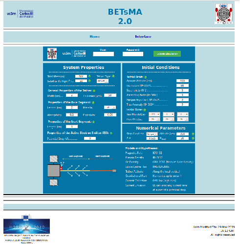
Figure 1: Web interface of BETsMA v2.0.

3. Adapting BETsMA to the Jovian environment

The most important modifications implemented in BETsMA v2.0 to address the analysis of EDT missions in Jupiter are the incorporation of models for the Jovian gravitational and magnetic [14] fields, and the plasma density [15]. The former is obviously necessary to compute the gravitational force, which is the dominant force affecting the dynamics of the tether system. Regarding the latter, i.e. the magnetic field and the plasma density, they are both essential for computing the current and voltage profiles along the tether and the Lorentz force. The thermal module that computes the tether temperature was also extended because it depends on the Sun-planet distance and the orbital period of the planet. 

4. Results and conclusion

This work presents a friendly software to simulate orbital maneuvers using EDTs in the Jovian environment. Key simulations and a comparison with more simple models used in the past are shown. The results also provide insight for planing future EDT missions to explore Jupiter's system. The software may be specially useful for non tether experts, who will be able to design their own missions without having a deep knowledge on tether modeling.   

Acknowledgments

This work has received funding from the European Unions Horizon 2020 research and innovation programme under grant agreement No 828902 (E.T.PACK project). GSA work is supported by the Ministerio de Ciencia e Innovación of Spain under the Grant RYC-2014-15357. 

References
[1] W. E. Hammond, S. E. Freeman, M. J. Nave, and C. C. Rupp, Jovian electrodynamic tether experiment, presented at the 29th Aerosp. Sci. Meeting, Reno, NV, Jan. 7-10, AIAA-91-0426 Paper. (1991).
[2] C. Bombardelli, E. C. Lorenzini, and J. R. Sanmartin, Jupiter Power Generation with Electrodynamic Tethers at Constant Orbital Energy, Journal of Propulsion and Power, vol. 25, n. 2. (2009).
[3] D. L. Gallagher, L. Johnson, J. Moore, and F. Bagenal, Electrodynamic Tether Propulsion and Power Generation at Jupiter, NasaTP-1998-208475. (1998).
[4] G. Lantoine, R.P. Russell, R.L. Anderson, H. B. Garrett, Magnetour: Surfing planetary systems on electromagnetic and multi-body gravity fields, Acta Astronauta, 138, 543-558. (2017).
[5] J. R. Sanmartin, J. Pelaez, and I. Carrera-Calvo, Comparative Saturn-Versus-Jupiter Tether Operation, Journal of Geophysical Research-Space Physics, 123, 7, 6026-6030. (2018).
[6] J. R. Sanmartin, and J. Pelaéz, Tether capture of spacecraft at Neptune, Acta Astronautica, in press. (2020).
[7] G. Sánchez Arriaga, C. Bombardelli, and X Chen, Impact of nonideal effects on bare electrodynamic tether performance, Journal of propulsion and power, 31(3), pp. 951-955. (2015).
[8] J. R. Sanmartin, M. Martinez-Sanchez and E. Ahedo, Bare wire anodes for electrodynamic tethers, Journal of Propulsion and Power, vol. 9, n. 3. (1993).
[9] The E.T.PACK Team, Electrodynamic Tether Technology for Passive Consumable-less Deorbit Kit. H2020 FET Open project No. 828902, www.etpack.eu.
[10] J. D. Williams, J. R., Sanmartín, L. P. Rand, Low workfunction coating for an entirely propellantless bare electrodynamic tether, IEEE Transactions on plasma science,40(5):1441-1445. (2012).
[11] G. Sanchez-Arriaga and Xin Chen, Modeling and Performance of Electrodynamic Low-Work-Function Tethers with Photoemission Effects, Journal of Propulsion and Power, vol. 34, n. 1. (2018).
[12] J. R. Sanmartin, R. D. Estes, E. C. Lorenzini, and S.A.Elaskar, Efficiency of Electrodynamic Tether Thrusters, Journal of Spacecraft and Rocket, vol. 43, n. 3. (2006).
[13] G. Sánchez-Arriaga and J. R. Sanmartin, Electrical model and optimal design scheme for low work-function tethers in thrust mode, Aerospace Science and Technology 96, 105519. (2020).
[14] K. K. Khurana, Euler potential models of Jupiter’s magnetospheric field, Journal of Geophysical Research: Space Physics, vol. 102, n. A6. (1997).
[15] F. Bagenal, R. J. Wilson, S. Siler, W. R. Paterson, and W. S. Kurth, Survey of Galileo plasma observations in Jupiter’s plasma sheet, Journal of Geophysical Research: Planets, vol. 121, n. 5. (2016).

How to cite: Borderes-Motta, G. and Sánchez-Arriaga, G.: BETsMA v2.0: A friendly software for the analysis of electrodynamic tether missions in Jupiter, Europlanet Science Congress 2020, online, 21 Sep–9 Oct 2020, EPSC2020-125, https://doi.org/10.5194/epsc2020-125, 2020.

During Cassini’s Grand Finale proximal orbits, the spacecraft traversed the nightside magnetotail to ~21 Saturn radii.  Clear signatures of Saturn’s equatorial current sheet are observed in the magnetic field data.  An axisymmetric model of the ring current is fitted to these data, amended to taken into account the tilt of the current layer by solar wind forcing, its teardrop-shaped nature and the magnetotail and magnetopause fringing fields.  Variations in ring current parameters are examined in relation to external driving of the magnetosphere by the solar wind, and internal driving by the two planetary period oscillations (PPOs) and compared with dawn and dayside regimes.  The relative phasing of the PPOs determines the ring current’s response to solar wind conditions. During solar wind compressions when the PPOS are in antiphase, magnetospheric storms are triggered and a thick partial ring current is formed on the nightside, dominated by hot plasma injected by tail reconnection.  However, during solar wind compressions when the PPOs are in phase, the magnetosphere shows only a ‘minor’ response and a partial ring current is not observed. During solar wind rarefactions an equatorial ‘magnetodisc’ configuration is observed in the dayside/dawn/nightside regions, with similar total currents flowing at these local times.  This partial ring current should close partly via magnetopause currents and possibly via field-aligned currents into the ionosphere.  During very quiet intervals of prolonged solar wind rarefaction, a thin current sheet with an enhanced current density is formed, indicative of a ring current dominated by cool, dense, Enceladus water group ions.

How to cite: Provan, G., Bradley, T., Bunce, E., Hunt, G., Cowley, S., Cao, H., Dougherty, M., Roussos, E., and Tao, C.: Saturn’s nightside ring current during Cassini’s Grand Finale , Europlanet Science Congress 2020, online, 21 Sep–9 Oct 2020, EPSC2020-213, https://doi.org/10.5194/epsc2020-213, 2020.

Between April and September 2017 in the final stages of the Cassini Saturn Orbiter mission the spacecraft executed 22 orbits passing planetward of the innermost ring, the D-ring.  During periapsis passes on all these orbits oscillations were detected in the azimuthal magnetic field components on typical time scales from a few minutes to 10 minutes. We argue that the time-varying signals detected on the spacecraft are also primarily time-varying in the plasma frame.  Nonetheless, we show that nearly all signals exhibit a distinct spatial effect, namely a magnetic node near the effective field line equator.  The oscillations thus have a standing structure along the background magnetic field and it follows that they are field line resonances associated with Alfvén waves.  The form of the signals suggests that the local field line resonances are most likely pumped from global sources.  This is the first detection in a giant planet magnetosphere of a phenomenon known to be important at Earth.

How to cite: Southwood, D., Cao, H., Hunt, G., Shebanits, O., and Dougherty, M.: Discovery of Alfven waves planetward of the Rings of Saturn, Europlanet Science Congress 2020, online, 21 Sep–9 Oct 2020, EPSC2020-365, https://doi.org/10.5194/epsc2020-365, 2020.

On February 7th 2018, during Juno’s 11th perijove observation sequence, Juno’s ultraviolet spectrograph (Juno-UVS) unveiled the development of a dawn storm in Jupiter's aurorae. These auroral events consist of spectacular brightenings of the midnight to dawn sector of the main emissions at Jupiter. At the end of the sequence, Juno crossed the magnetic field lines connected to this dawn storm, unraveling some of the processes giving rise to these spectacular events.
All in situ instruments detected a sharp transition as the spacecraft entered the dawn storm at an altitude of approximately 5RJ in the southern hemisphere. The particle fluxes detected by the JADE and JEDI instruments, including electrons and ions, increased dramatically. A strong flux of penetrating radiation was also detected by the UVS instrument. The Alfvén waves spectrograms derived from the MAG instrument also show a clear transition between a quiet and an extremely active regime as the spacecraft entered the dawn storm. Furthermore, the orientation of the magnetic field showed a very strong perturbation, associated with intense currents. And, finally, intense bKOM emissions were also observed during this time interval. Combined with the remote sensing observations of the aurora, these datasets strongly suggest that Juno witnessed a strong magnetospheric reconfiguration that started in the magneto-tail and then evolved toward dawn as the planet rotated.

How to cite: Bonfond, B., Guo, R., Yao, Z., Denis, G., Gérard, J.-C., Randy, G., Vincent, H., Thomas, G., Versteeg, M., Kammer, J., Allegrini, F., Ebert, R., Kurth, W., Louarn, P., Gershman, D., Connerney, J., Kotsiaros, S., and Mauk, B.: Flying through a dawn storm: a multi-instrument study of the traversal of a dawn storm by Juno on February 7th 2018, Europlanet Science Congress 2020, online, 21 Sep–9 Oct 2020, EPSC2020-270, https://doi.org/10.5194/epsc2020-270, 2020.

Saturn's magnetosphere is an efficient emitter of Energetic Neutral Atoms (ENAs), given the presence of an extended neutral cloud around the planet that originates from the icy moon, Enceladus. The ENA emission is symptomatic of the global circulation of plasma in Saturn's magnetosphere. Energetic ions are injected from the outer magnetosphere following magnetotail dynamics and reconnection events. These ions then charge exchange with the neutral cloud, which is mostly confined to the spin plane, resulting in ENA production. The global ENA emission is dynamic, displaying sudden brightening on the nightside, and discrete rotating enhancements which circle the planet for many hours as energetic ions drift with the bulk plasma flow. These latter features have been linked with rotating signatures in the ultraviolet auroras, suggesting coupling via some transient system of field-aligned currents that forms following injection events. Indeed these injection events occur so often as to form Saturn’s dawn auroral arc.

Our characterization of the ENA emission at Saturn is made possible using imagery from the Ion-Neutral Camera (INCA) that flew onboard Cassini. Observations were made over the entire mission lifetime. We present for the first time a statistical analysis of the complete INCA image set, using equatorial projections of the flux distribution to reveal the time-averaged morphology of Saturn's ENAs. 

We used a comprehensive data processing and equatorial projection algorithm to calibrate, clean and filter for all high inclination orbit days. In the final average pictures, many of the projected pixels consist of between tens to hundreds of days continuous exposure, all captured with a line-of-sight > 50° elevation (above the projection plane) and within 30 R_S distance from the spacecraft.

We find clear toroidal ENA distributions in O and H, and all INCA energy bands, with the emission dropping off sharply inside 5 R_S radial distance in all cases. Average peak intensities occur at radial distances from ~7 R_S (O, 170-230 keV) to ~10 R_S (H, 24-55 keV). All toroids are offset towards the dayside by several R_S, most clearly in the 24-55 keV H image, with a maximum intensity at ~13-14 R_S from the planet centre on the dayside, compared to only ~10 R_S on the nightside. The H ENA distribution is also enhanced around midnight local times, as previously observed in an early morphological study of 2007 data by Carbary et al. [2008], a net effect associated with reconnection return flows and transient ENA enhancements in this sector.

We also explore possible organisation of the average global ENA intensity by Saturn’s rotating current systems associated with planetary period oscillations (PPOs, e.g., Provan et al. [2018]). We find that the ENA intensity is statistically modulated by periodic changes in expected plasma sheet thickness as controlled by field-aligned current interactions, a pattern evident in both north and south rotating system frames. With a thicker plasma sheet, more energetic ions are available to charge exchange within the background neutral cloud, and the LOS integral measure increases as a result (and vice versa). In this long-term picture, this effect may dominate over other possible PPO modulation effects on the appearance or evolution of transient ENA injection signatures.

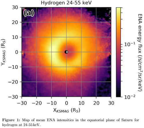
How to cite: Kinrade, J., Bader, A., Badman, S., Paranicas, C., Constable, D., Arridge, C., Cowley, S., Provan, G., and Mitchell, D.: The statistical morphology of Saturn’s equatorial ENA projections, Europlanet Science Congress 2020, online, 21 Sep–9 Oct 2020, EPSC2020-287, https://doi.org/10.5194/epsc2020-287, 2020.

Magnetic flux ropes – helical magnetic structures which are produced due to simultaneous reconnection at multiple X-lines, have been observed at the magnetospheres of most magnetized planets. The size of these flux ropes, also called “plasmoids” if they contain significant plasma pressure, can vary from being a significant fraction of the system size (e.g. tens of Earth radii at the terrestrial magnetotail) to small flux ropes with diameters less than the local ion inertial length. The smallest flux ropes are expected because reconnection in the Earth’s cross-tail current sheet only occurs when it thins to or below the ion-inertial scale and tearing instabilities produce periodic X-lines with spacing of ~2 times the thickness of the current sheet. While much is still to be understood, it is hypothesized on the basis of Particle-in-Cell simulations that the smaller flux ropes soon come together and “coalesce”, via reconnection, into larger flux ropes. The coalescence process continues until the observed distribution of plasmoid diameters is produced.

For the giant magnetospheres like Jupiter, which encompass multiple moons that lose mass to the rapidly rotating inner plasma disk, the momentum in the outer layers of the disk is believed to continuously shed mass by the release of plasmoids down the tail plasma sheet. This periodic ejection of plasmoids to balance the mass being added to the magnetosphere by Jupiter’s moons is termed the Vasyliunas-cycle. Rather than being formed by multiple x-line reconnection in a highly thinned current sheet, these Vasyliunas-cycle plasmoids are thought to form when a single X-line disconnects a highly stretched closed flux tube and allows its momentum to carry it down the tail. Due to the limited single-spacecraft measurements obtained by Galileo in the dusk-side magnetosphere, relatively little is known about these Vasyliunas-type plasmoids. Signatures of most Jovian plasmoids and flux ropes lasted ~6.8 minutes on average (Vogt et al., 2014), corresponding to diameters larger than 1 Jovian radii (R_J); much larger than the ion inertial length expected in the outer magnetosphere. Potential flux ropes on the ion-inertial scale, which would typically last for less than a minute could not have been identified using the Galileo magnetometer owing to the low cadence of several seconds per vector measurement.

As part of its 53-day orbits, Juno spent a considerable amount of time in the dawn-side magnetotail. Using the high-resolution data from the Juno magnetometer, we identified two potential ion-scale flux ropes in the Jovian magnetotail by searching for bipolar variations in the magnetic field component normal to the current sheet. The two events were 22 s and 62 s in duration and were located at radial distances of roughly 74 R_J and 92 R_J between 03 and 04 local time. Assuming that the travel speed of the flux rope is limited by the Alfven speed in the surrounding magnetotail lobes, which is calculated using the plasma density inferred by the cutoff for the continuum radiation detected by the Waves instrument (0.003 to 0.012 cm^-3), we estimated the diameters of these flux ropes to be 0.14 and 0.19 R_J respectively. The flux ropes’ diameters were comparable to the ion inertial length during these intervals, which was roughly between 0.11 to 0.23 R_J, (assuming a mass of 16.6 amu for the average ion). The selected events were analyzed using the minimum variance analysis and both events were seen to possess a strong core field with relatively high eigenvalue ratios, indicating that the MVA coordinate system was well-defined. Using a force-free model which is fitted to the observations, it was found that the flux ropes are quasi-force-free.

These are the first reported observations of ion-scale flux ropes in the Jovian magnetotail. Although the large-scale dynamics of the magnetosphere may be dominated by the Vasyliunas cycle, the observations show that small-scale flux ropes, which are likely generated due to the tearing instability in a thin current sheet, also exist in the Jovian magnetotail, similar to the magnetotails of Earth and Mercury.

How to cite: Sarkango, Y., Slavin, J. A., Jia, X., DiBraccio, G. A., Gershman, D. J., Connerney, J. E. P., Kurth, W. S., and Hospodarsky, G. B.: Juno Observations of Ion-Inertial Scale Flux Ropes in the Jovian Magnetotail, Europlanet Science Congress 2020, online, 21 Sep–9 Oct 2020, EPSC2020-520, https://doi.org/10.5194/epsc2020-520, 2020.

Jovian magnetosphere has   a huge equatorial plasma disk, which is also known as the current sheet or magnetodisk. This current sheet enlarges the subsolar magnetosphere size more than twice compare to purely planetary dipole magnetosphere. Near to the planet   the magnetodisk is aligned with the magnetic equatorial plane. As consequence of the dipole axis tilted to the polar axis about 10, each of Juno orbits crossed the central surface of the disk current two times during one jovian day (9, 92 hours). Finally, we have  about 1725 current sheet crossings to study the plasma sheet and current sheets structure.

In our work we have developed a database of Jovian current sheet crossings, performed by Galileo and Juno spacecraft, which includes magnetic field and plasma measurements. Current sheet crossings were determined using magnetometer data in distant magnetosphere as a region with the magnetic field strength less than the dipole value at the same point and central current sheet position have been marked by boundary between the region with opposite signum of the radial magnetic field component.

How to cite: Alekseev, I., Belenkaya, E., Lavrukhin, A., Parunakian, D., and Pensionerov, I.: Development of a database of Jovian magnetodisc crossings by Galileo and Juno spacecraft from magnetometer data, Europlanet Science Congress 2020, online, 21 Sep–9 Oct 2020, EPSC2020-615, https://doi.org/10.5194/epsc2020-615, 2020.

In this work, the locations of observed Ganymede’s magnetic footprint were compared with the locations predicted by the magnetic field model under different plasma conditions. The shifts of Ganymede's magnetic footprint locations from average footpath given by Grodent et al. (2008) were analyzed. The average path is created from about 1000 images taken by instruments onboarded Hubble Space Telescope (HST). The position shifts indicate the variation of magnetic field line mapping from Ganymede to Jupiter’s ionosphere. The two sets of data from HST were analyzed to obtain the locations of Ganymede’s magnetic footprint in 2007 and 2016. For both sets of data, at longitude ranging approximately from 170° to 180°, we found that the locations were significantly shifted in poleward direction between 0.5° to 2° from the average footpath. Different from data in May 2007, the Ganymede’s magnetic footprint locations in May 2016 at longitude about 160° could possibly locate in equatorward direction. At orbital distance of Ganymede about 15 R_J, in Jupiter’s middle magnetosphere, there is strong influence of plasma, whose major source is Io’s volcanic eruptions. Thus, the variations of plasma resulting in the stretching of magnetic field lines affect the magnetic field mapping from Ganymede to ionosphere. Furthermore, based on the magnetodisc model, the hot plasma pressure anisotropy strongly influences the stretching of the field lines and the mapped locations of Ganymede’s footprint in ionosphere to be shifted in either poleward or equatorward directions. In this study, we detected both poleward and equatorward shifts in different observations, whose connection with the plasma environment in the middle magnetosphere awaits for further study.

How to cite: Promfu, T., Wannawichian, S., Nichols, J., and Clarke, J.: Ganymede’s magnetic footprint mapping: Modeling and HST observations, Europlanet Science Congress 2020, online, 21 Sep–9 Oct 2020, EPSC2020-105, https://doi.org/10.5194/epsc2020-105, 2020.

Electrons in Saturn's radiation belts are distributed along discrete energy bands, a feature often attributed to the energisation of charged particles following their rapid injection towards a planet's inner magnetosphere. However, the mechanism that could deliver electrons deep into Saturn's radiation belts remains elusive, as for instance, the efficiency of magnetospheric interchange injections drops rapidly for electrons above 100 keV and at low L-shells. Using Cassini measurements and simulations we demonstrate that the banding derives from slow radial plasma flows associated to a persistent convection pattern in Saturn's magnetosphere (noon to midnight electric field), making the need for rapid injections obsolete. This transport mode impacts electron acceleration throughout most the planet's radiation belts and at quasi and fully relativistic energies, suggesting that this global scale electric field is ultimately responsible for the bulk of the highest energy electrons near the planet. We also present evidence from Galileo and Juno that the influence of Jupiter's inner magnetospheric convection pattern on its radiation belts is fundamentally similar to Saturn's but affects its higher energy ultra-relativistic electrons. The comparison of the two radiation belts indicates there is an energy range above which there is a transition from interchange to global scale electric field driven electron acceleration. This transiroty energy range can be scaled by the two planets' magnetic moment and strength of corotation, allowing us to study these two systems in complement.

How to cite: Roussos, E., Hao, Y., Sun, Y., Liu, Y., Kollmann, P., Yuan, C., Krupp, N., Paranicas, C., Zhou, X.-Z., Murakami, G., Kita, H., and Zong, Q.: Relativistic electron acceleration at Saturn and Jupiter by global scale electric fields, Europlanet Science Congress 2020, online, 21 Sep–9 Oct 2020, EPSC2020-723, https://doi.org/10.5194/epsc2020-723, 2020.

At Jupiter, part of the auroral radio emissions are controlled by the Galilean moons Io, Europa and Ganymede. Until now, they have been remotely detected using ground-based radio-telescope or electric antenna aboard spacecraft. The polar trajectory of the Juno orbiter leads to cross the magnetic flux tube connected to these moons, or their tail, and gives a direct in-situ measurements of the characteristics of these decametric moon induced radio emissions (such as the electron population, size of the source, and beaming angle and growth rate of the emission). In this study, we focus on the crossing of the Ganymede flux tube. The study of Juno/JADE-E and Juno/Waves data leads to an estimated source size of a few 100s km, an electron population of energy E= 8±2 keV and an emission beaming angle of θ= 80±2° from the magnetic field lines. Finally, this crossing of a decametric radio emission induced by a moon brings us new constrains on the Cyclotron Maser Instability process

How to cite: Louis, C., Louarn, P., Kurth, W., Allegrini, F., and Szalay, J.: Ganymede-induced decametric emission: in-situ measurements by Juno., Europlanet Science Congress 2020, online, 21 Sep–9 Oct 2020, EPSC2020-763, https://doi.org/10.5194/epsc2020-763, 2020.