TP1

Summary:

We investigated the Yarkovsky-O’Keefe-Radzievskii-Paddack (YORP) effect [Rubincam 2000] acting on asteroid (162173) Ryugu. To accurately simulate the thermal condition on Ryugu, we employed a thermophysical model recently developed by Nakano and Hirabayashi [2021], which considers self-heating effect and scattering of radiation and solves the 3-dimensional heat equation via Finite Element Modeling (FEM) approach. Our result indicates that on 1 August 2018 TDB, the thermal torque (YORP torque) was acting in a direction that accelerates Ryugu’s spin rate.

Introduction:

Dynamics of small bodies among the near-Earth and main belt asteroids are controlled by secular effects due to thermal radiation forces and torques, known as the Yarkovsky and YORP effects [Rubincam 2000; Vokrouhlický and Čapek, 2002, Bottke et al., 2006]. Recent increase in the number of observed top-like shape objects suggests that the YORP effect is a key mechanism for their spin rates acceleration (or deceleration), which can induce mass-shedding or catastrophic disruptions [e.g., Holsapple, 2010; Hirabayashi, 2015]. Thus, modeling the Yarkovsky and YORP effects based on a proper thermophysical technique is one of the crucial steps to understand their formation and evolution mechanisms. Here, we investigate the YORP effect on asteroid (162173) Ryugu by using a thermophysical model recently developed by Nakano and Hirabayashi [2021].

Thermophysical modeling of Ryugu:

Unlike earlier thermophysical models which typically solve the 1-dimensional heat equation, the FEM approach thermophysical model solves the 3-dimensional heat equation. It considers the self-heating and scattering of radiation, similar to other models [e.g., Rozits and Green, 2011; Davidsson and Rickman, 2014]. The surface boundary condition includes: direct solar flux U, diffuse solar radiation flux W, direct self-heating u, and diffuse self-heating w [Davidsson and Rickman, 2014]. To efficiently describe the surface/subsurface thermal evolution, “layer” FEM shape model, where only the layers of tetrahedral meshes exist for the surface and subsurface, and the inside is left as cavity, is used. (See Nakano and Hirabayashi [2021] for more detail.)

We retrieved Ryugu’s ephemeris and the sun’s position vector as seen from Ryugu on 1 August 2018 TDB, using a SPICE kernel for Ryugu. The orbital elements and physical parameters used in this investigation are listed in Table 1. The layer FEM shape model was constructed based on SFM_49k_v20180804 [Watanabe et al., 2019], but the number of facets was decreased from 49k to 4.9k. Figure 1 shows the surface temperature distribution on Ryugu obtained after 25 spins (≈190 hr) at the fixed distance from the Sun. The surface temperature distribution is comparable to that observed by Hayabusa2 spacecraft [Okada et al., 2020].

The YORP effect on Ryugu:

Once the surface temperature is obtained, a recoil force df due to reflected solar and thermally radiated photons for each facet can be computed [Rozits and Green, 2012]. Assuming Lambert (isotropic) emission from the surface, it is given by [Vokrouhlický and Čapek, 2002; Rozits and Green, 2012]:

where ε is the emissivity of the surface, σ is the Stefan-Boltzmann constant, T is the surface temperature, G is reflected scattered flux, c is the speed of light, and dS is the facet area. The net torque τ acting on Ryugu can be computed by taking a cross product of the facet position r and the recoil force df for each facet and integrating it over the whole surface:

The net torque computed by the above equation can be decomposed into three meaningful YORP torque components of our interest: a spin period change component τ_ω, a spin pole obliquity change component τ_ε, and a precession of rotation τ_ψ (see e.g., Bottke et al., 2006 for the equations). Figure 2 shows the time history of YORP torque components over one Ryugu’s spin. The one-spin averaged YORP torque components are found to be:

Discussion:

Due to its top-like asymmetric shape, Ryugu should be susceptible to the YORP effect. Our investigation with the 3-dimensional thermophysical modeling technique clearly showed that Ryugu does experience non-negligible YORP effect. While the YORP torque components change their signs during one spin (Figure 2), the one-spin averaged values were all found to be positive. In particular, the positive  implies an increase of Ryugu’s spin rate. This contradicts with the current hypothesis that Ryugu spun faster in the past and later slowed down to the current spin state [Watanabe et al., 2019]. In this investigation, however, we only explored Ryugu’s thermal condition at a particular epoch. Therefore, we cannot infer Ryugu’s secular dynamical evolution. The YORP effect may be highly sensitive to small topographic features on the surface [Statler, 2009]. The surface roughness may also affect thermal evolutions [Shimaki et al., 2020]. We plan to expand our modeling technique to investigate such effects and to further constrain the Yarkovsky and YORP effects on small bodies.

Table 1. List of parameters used in this investigation

Figure 1. Surface temperature distribution on 1 August 2018 TDB

Figure 2. YORP torque components versus time

Acknowledgments: RN and MH acknowledge support from NASA/Solar System Workings (NNH17ZDA001N/80NSSC19K0548) and Auburn University/Intramural Grant Program.

References:

Bottke et al. (2006) Annu. Rev. Earth Planet. Sci., 34; Davidsson and Rickman (2014), Icarus, 243; Hirabayashi (2015) MNRAS, 454; Holsapple (2001) Icarus, 154; Nakano and Hirabayashi (2021) 52^nd LPSC, 1292; Okada et al. (2020) Nature, 579; Rozits and Green (2011) MNRAS, 415; Rozits and Green (2012) MNRAS, 423; Rubincam (2000) Icarus, 148; Shimaki et al. (2020) Icarus, 348; Statler (2009) Icarus, 202; Vokrouhlický and Čapek (2002) Icarus, 159; Watanabe et al. (2019) Science, 364

How to cite: Nakano, R. and Hirabayashi, M.: Investigation of the YORP effect on asteroid (162173) Ryugu – An application of FEM approach thermophysical model, Europlanet Science Congress 2021, online, 13–24 Sep 2021, EPSC2021-441, https://doi.org/10.5194/epsc2021-441, 2021.

Abstract

We present here a method for the retrieval of the internal density distribution of a small body, via a least squares inversion of its gravity field and rotational state. Multiple solutions are averaged in order to limit the effect of the a priori density distribution. Simulations show successful density map estimations even with little to no initial information on the interior structure of the body.

1. Introduction

The gravity field of a body is a property among the most readily obtainable by a spacecraft mission. Be it by employing radio-tracking, optical, or gravimetric data, several missions have provided and will provide gravity expansions of degree 2 and higher for small bodies. In turn, the extended gravity field is an effect of the distribution of the mass inside the body. However, the inverse problem of estimating the density distribution from the gravity field is not a trivial one, and generally with non-unique solutions [1].

Here, we propose a method to obtain a unique solution for the internal mass distribution of a small body by restricting our estimation to zones of constant density, which are limited in number by the accuracy of the gravity model [2]. Where available, additional observables such as the libration amplitudes could help in the estimation of the interior structure. Averaging of the solutions obtained for different subdivisions of zones provides then the estimated density map [3].

2. Methods

The code builds from available software which allows to compute the gravity harmonics of a body approximated by a collection of cubes, each with a given density [4]. Here, the cubes are grouped in subregions of constant density, as many as there are measured coefficients. Each subregion is assigned an initial density, from which the software computes gravity coefficients matching in degree and order those observed. The difference between the coefficients thus computed and the observed ones is then minimized in a least-squares sense [5]. The solution of the regularized least-squares inversion is the density for each of the initial zones, along with its uncertainty. However, this solution is heavily dependent on the initial subdivision of the body into zones. Hence, a wide range of possible initial zones is explored, and the corresponding density solutions averaged together. 

From such an average solution, a new set of subregions is generated, with the help of a blob detection algorithm [6]. Finally, the gravity coefficients are inverted using this new zone subdivision. This step is necessary because, while providing a good distribution of the density zones, the density values of the averaged map are biased by solutions coming from inaccurate initial zones subdivisions. 

The data used in the inversion are the spherical harmonics coefficients of the gravity field expansion. The advantage of these observables is that they can be measured without the need for specific payload. Although the method can be easily adapted to process surface gravity measurements, the larger errors on the surface gravity coming from the cubes discretization make it less appealing for these type of data.

3. Discussion and outlook

Figure 1 shows the results obtained when applying the method to a fictitious density distribution for asteroid Bennu. The nominal density distribution, shown in Figure 1a, was used to produce a synthetic gravity field expansion of degree 11. An optimistic noise profile was assumed for these simulated observables, with a 1% error on each gravity coefficient. The spherical harmonics coefficients were then inverted via the iterative process described in Section 2, resulting in the density distribution shown in Figure 1b. 

With a gravity field of this resolution, the inversion method is clearly able to distinguish the 4 density anomalies inside the body. Still, the comparison between the nominal and the estimated density models reveals the current limitations of the method in accurately reconstructing the size of the anomalies or their density — which is equivalent, given the constraint on the total mass. 

Once a better agreement between the retrieved and the nominal models will be achieved with the current (high) resolution of the gravity harmonics, the synthetic gravity fields will be truncated at lower degrees, making them more realistic as outputs of spacecraft missions to small bodies. Future simulation studies will also make use of more realistic noise profiles, with the errors on the observed coefficient increasing as a function of the degree.

(a)

(b)

Figure 1: (a) density model used to simulate a degree-11 gravity field; (b) density distribution retrieved from said gravity field, without any initial assumptions about the true distribution

Acknowledgements

This work was financially supported by the French community of Belgium within the framework of a FRIA grant, and by the Belgian PRODEX program, managed by the European Space Agency in collaboration with the Belgian Federal Science Policy Office.

References

[1]  P. Tricarico. Global gravity inversion of bodies with arbitrary shape. Geophysical Journal International, 195(1):260–275, 2013.
[2]  Y. Takahashi and D. J. Scheeres. Morphology driven density distribution estimation for small bodies. Icarus, 233:179–193, 2014.
[3]  L.-I. Sorsa, M. Takala, P. Bambach, et al. Tomographic inversion of gravity gradient field for a synthetic Itokawa model. Icarus, 336:113425, 2020.
[4]  S. Le Maistre, A. Rivoldini, and P. Rosenblatt. Signature of Phobos’ interior structure in its gravity field and libration. Icarus, 321:272–290, 2019.
[5]  D. J. Scheeres, B. Khushalani, and R. A. Werner. Estimating asteroid density distributions from shape and gravity information. Planetary and Space Science, 48(10):965–971, 2000.
[6]  S. v. d. Walt, J. L. Schönberger, J. Nunez-Iglesias, et al. scikit-image: image processing in Python. PeerJ, 2:e453, 2014.

How to cite: Caldiero, A., Le Maistre, S., and Dehant, V.: Estimation of the interior density of a small body given its gravity field, Europlanet Science Congress 2021, online, 13–24 Sep 2021, EPSC2021-756, https://doi.org/10.5194/epsc2021-756, 2021.

The binary asteroid 65803 Didymos-Dimorphos is the target of NASA’s DART (Cheng et al., 2018) and ESA's Hera missions (Michel et al., 2018). Hera will arrive at the asteroid system several years after the DART impact. It will carry out a detailed characterisation of the asteroids’ overall properties and will measure the outcome of the DART impact on Dimorphos. 

Didymos, the primary body, is a fast spinning asteroid with a period of only 2.26 hours, which is very close to the critical spin limit of 2.2 hours for asteroids bigger than approx. 200 m (Walsh et al., 2018). The interior structure of Didymos is crucial for our understanding of its stability. Without cohesion and with an estimated bulk density of 2.1 g/cc, Didymos is not able to keep its shape stable (Holsapple, 2001; Zhang et al., 2017) and thus, cohesive forces might be present in its structure.

The interior strength properties of asteroids determine to a large degree their collisional evolution. For small bodies, even a small level of cohesion can significantly affect the outcome of an impact  (Raducan and Jutzi, 2021). 

Previous studies have applied N-body and soft-sphere discrete element (SSDEM) codes to study the structural stability of rubble pile asteroids (Sanchez and Scheeres, 2012; Zhang et al., 2017, 2021; Ferrari and Tanga, 2020). Recently, the stability and failure modes of such objects have been studied using finite element (FEM) (Hirabayashi et al., 2020). Here we use Bern’s Smooth Particle Hydrodynamics (SPH) code (Jutzi et al., 2008; Jutzi 2015) to simulate the rotating asteroid and to investigate its physical properties. To do this, we set up Didymos according to its recent shape model (provided by the Hera Didymos Reference Model) with a bulk density of 2.1 g/cc and we spin up the body to a rotation period of 2.26 hours.

For the preliminary simulations presented here, we assume that Didymos has a homogeneous structure. We perform simulations using a range of values for the cohesion and the internal friction coefficient of the asteroid, and then for each case we evaluate Didymos’ stability.

An example of such a simulation is shown in Figure 1. For a cohesion of 100 Pa and a friction coefficient of 0.4, we find that Didymos’ shape is stable and only very little deformation takes place, as indicated by the small values in the total accumulated strain. In Figure 2, we show the case with a lower cohesion of 0.1 Pa and a coefficient of friction of 0.4. In this case, Didymos experiences large-scale deformations. To quantify the degree of deformation, we compute the cumulative strain distributions for both cases (Figure 3). For the 100 Pa cohesion case, > 90 % of the total mass experiences a total strain of < 0.03 and therefore this case is considered to be stable. On the other hand, for the case with 0.1 Pa cohesion, > 50 % of the total mass experiences a total strain of > 0.5, consistent with the large scale deformations observed in Figure 2. 

Our initial results suggest that a cohesion of ~ 10-100 Pa is required to maintain structural stability, which is consistent with recent SSDEM modeling results (Zhang et al. 2021). 

However, so far only homogeneous structures have been explored. We plan to investigate also more complex interior structures that may lead to different outcomes in terms of required cohesion to obtain an overall structural stability. 

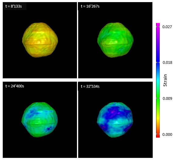
Figure 1: Surface of Didymos after spin-up is complete, for a friction coefficient of 0.4 and a cohesion of 100 Pa. The body is shown from the same side at four different times. The body experiences only very little deformation, as indicated by the small amount of accumulated strain.

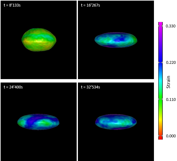
Figure 2: same as Figure 1, but this time for a friction coefficient of 0.4 and a cohesion of 0.1 Pa. The body gets deformed already before the spin-up is completed.

Figure 3: Cumulative strain distribution for the two simulations shown in Figures 1 and 2. The strain experienced by the body with a cohesion of 100 Pascal (a) is much smaller than for the body with a cohesion of 0.1 Pa (b).

Acknowledgements:

This work has received funding from the European Union’s Horizon 2020 research and in- novation programme under grant agreement No. 870377

References:

Cheng, A. F., et al. (2018) Planet. Space Sci., 157, 104-115.

Jutzi, M. et al. (2008) Icarus, 198:242–255

Jutzi, M. (2015) Planet. Space Sci., 107:3–9. 

Ferrari, F. and Tanga P. (2020) Icarus, 350.

Hirabayashi et al. (2020) Icarus, 352.

Holsapple (2001) Icarus, 154, 432-448.

Michel, P., et al. (2018) Adv. in Space Res., 62 (8), 2261-2272.

Raducan, S. D. and Jutzi, M. (2021) LPSC, (2548):1900.

Sanchez, D. P. and Scheeres, D. J. (2012) Icarus, 218, 876-894.

Sugiura et al. (2021) Icarus, https://doi.org/10.1016/j.icarus.2021.114505

Walsh, K. J. (2018) Annu. Rev. Astron. Astrophys., 56, 593-624.

Zhang, Y., et al. (2017) Icarus, 294, 98-123.

Zhang, Y., et al. (2021) Icarus 362, http://doi.org/10.1016/j.icarus.2021.114433

How to cite: Hauser, I., Jutzi, M., Raducan, S. D., and Ferrari, F.: Structural stability of 65803 Didymos: insights from SPH simulations, Europlanet Science Congress 2021, online, 13–24 Sep 2021, EPSC2021-483, https://doi.org/10.5194/epsc2021-483, 2021.

Introduction

(65803) Didymos is a binary asteroid that orbits the Sun having a semi-major axis of 1.64 AU and is the target of the DART (NASA) and Hera (ESA) missions. The system is made up of a 780 m diameter primary body (Didymos) and a 160 m satellite (Dimorphos), orbiting the primary with a semi-major axis of 1180 m and an orbital period of 11.9 h [1]. The primary has a rotation period of 2.26 h, very close to the limit of structural stability [2] [3]. The low density estimated for Didymos, 2170 kg/m³, shows that it is not a monolithic body but instead has a high macroporosity, typical of gravitational aggregates or rubble-piles. Numerical simulations show that they can be generated naturally in the aftermath of a catastrophic collision between asteroids, as a result of the gravitational interaction between the irregular fragments resulting from the collision [4]. The evolution under YORP spin-up may lead in the same case to oblate spheroidal shape asteroids with an equatorial bulge [5], commonly called top-shapes (eg: (162173) Ryugu [6], (101955) Bennu [7], (65803) Didymos, etc.). These bodies may rotate close to the limit of structural stability, kept together by the shear forces generated by friction between their components. The local acceleration near the equatorial regions may be directed outwards in these asteroids, allowing regolith to leave the surface [8] [9]. When this happens, particles evolve under the action of the gravitational field of the asteroid, the gravitational force of the Sun, the pressure of solar radiation, and in the case of binary asteroids, the secondary’s gravitational force intervene as well.

Methodology

In this work, we study the dynamics of the particles that are ejected from the surface of Didymos when the centrifugal acceleration is large enough to overcome local gravity. The analysis is carried out from the development of a numerical code that integrates the particles’ equation of motion in a rotating frame of reference, centered on the primary asteroid. A polyhedral shape model for Didymos is considered, formed by 1000 vertices and 1996 triangular faces, in which centers particles are placed. Particle size distribution is generated by a power law n(r)=kr^α with an index set as α=-3.5. The environment of the asteroid is studied by computing the radial density of particles. To do this, a 3D grid is built; the surface is divided into bins of latitude and longitude and is propagated in radial bins. A process of detachment and re-entry of particles to the primary is observed, which could promote the potential formation of dust bands in the equatorial region of the asteroid. Trajectories are analyzed and the percentage of particles that re-accumulate on the secondary and the ones that completely escape the system are calculated.

References

[1] Benner, L. A. et al. Radar imaging and a physical model of binary asteroid 65803 Didymos. Bull. Am. Astron. Soc. 42, 1056 (2010).

[2] Pravec, P. and 30 colleagues 2008. Spin rate distribution of small asteroids. Icarus 197, 497–504.doi:10.1016/j.icarus.2008.05.012

[3] Margot, J.-L., Pravec, P., Taylor, P., Carry, B., Jacobson, S. 2015. Asteroid Systems: Binaries, Triples, and Pairs. Asteroids IV 355–374. doi:10.2458/azuuapress9780816532131-ch019

[4] Campo Bagatin, A., Alemañ, R.A., Benavidez, P.G., Richardson, D.C., 2018. Internal structure of asteroid gravitational aggregates. Icarus 302, 343–359.

[5] Cheng, B. and 7 colleagues 2021. Reconstruct-ing the formation history of top-shaped asteroids from thesurface boulder distribution. Nature Astronomy 5, 134–138.doi:10.1038/s41550-020-01226-7

[6] Watanabe, S. et al. Hayabusa2 arrives at the carbonaceous asteroid 162173 Ryugu—a spinning top-shaped rubble pile. Science 364, 268–272 (2019).

[7] Lauretta, D. S. et al. The unexpected surface of asteroid (101955) Bennu. Nature 568, 55–60 (2019).

[8] Campo Bagatin, A. 2013. Small Asteroids with “Dusty” Atmospheres?. Lunar and Planetary Science Conference.

[9] Yu, Y., Michel, P., Hirabayashi, M., Richardson,D. C. 2019. The expansion of debris flow shed from the primary of 65803 Didymos. Monthly Notices of the Royal Astronomical Society 484, 1057–1071. doi:10.1093/mnras/sty3515

How to cite: Trógolo, N., Moreno, F., Campo Bagatin, A., and Pérez Molina, M.: Analysis of the dynamical evolution of lofted particles around (65803) Didymos asteroid, Europlanet Science Congress 2021, online, 13–24 Sep 2021, EPSC2021-676, https://doi.org/10.5194/epsc2021-676, 2021.

The Austrian contribution to Phase B2 Part 1 of HERA mission [1] was carried out in 2020 by JR, VRVis, and two science collaborators under GMV contract. It mainly consisted of the design of tools needed to determine Didymain´s shape [2], [3]. The challenges to be faced in Phase B2 Part 2 of the mission are focussed on Dimorphos 3D reconstruction and must be carried out within the timeframe January-June 2021, therefore some parts are still not finalised. These challenges consist of:

• Parameter definition to optimize Dimorphos imaging to support HERA science return sequence
• Rendering of Didymos images with PRo3D along COP (Core Operations Phase) trajectory
• Dimorphos 3D reconstruction with ColMap [7] using the simulated images along the COP trajectory
• Implementation of evaluation parameters in PRo3D [4] to assess Dimorphos´ reconstruction accuracy

Dimorphos images optimization

The main objective of this task is to obtain the best HERA AFC images of Dimorphos along the COP trajectory. At the same time, the maximal number of images for daily downlink must be considered as it is limited to 16 images per day. Due to the downlink data restriction the images must be optimised by selecting predetermined HERA acquisition times that provide the best imaging of Dimorphos. Therefore, images where Dimorphos appears completely occluded by Didymain, as well as images where the small asteroid is outside the AFC FoV, must be avoided for downlink and reconstruction. To recognise these images, the parameter angular deviation “α” between Didymain (Dd) and Dimorphos (Dm) was defined and the diagonal FoV of the HERA AFC was considered. The calculation and pseudocode to classify if an image should be rendered are displayed in Equation 1 and are based on HERA SPICE kernels.

Image rendering of Dimorphos

To generate synthetic images of Dimorphos in the most representative and faithful way, the information about the geometry of the Asteroid Frame Camera (AFC), its positions and orientations along the COP trajectory, and a celestial body of shape parameters similar to Dimorphos had to be considered. For the last, a 3D model of the Itokawa asteroid was textured and scaled along the three axes to get Dimorphos similar size. The resulting “*.opc” file can be seen on the left side of Figure 1. For Didymain, the same body approximation taken for Part 1 of the project was used (Figure 1,  right).

For image rendering the time interval was set to 10 min, as required by GMV, and the PRo3D Viewer [4] was used and interfaced via a “.json” file. As already mentioned, only the images selected with both criteria (angular deviation and AFC FoV) were rendered. An example of the resulting images for COP trajectory in timeframe 2024 (2027-05-22) can be seen in Figure 2:

Dimorphos Shape reconstruction

To determine Dimorphos’ shape, the images rendered with PRo3D are supplied to the ColMap [7] tool, embedded in PRoViP [5]. ColMap performs 3D reconstruction by means of Structure from Motion (SfM). In order to establish correct SfM conditions, all AFC poses and orientations calculated with the SPICE kernels must be transformed with the inverse rotations of Dimorphos to simulate a moving camera around a static scene. Then, the new transformation matrices and the AFC parameters are provided to ColMap [2], [3]. The sequence for 3D reconstruction is as follows:

• Image features extraction (Figure 3, left)
• Image features matching (Figure 3, right)
• Triangulation of sparse image features
• Images´ preparation for dense matching
• Dense depth maps generation
• Fuse dense depth maps
• 3D mesh generation

Reconstruction evaluation

For reconstruction evaluation, the resulting 3D model must be compared to the initial one used for images simulation. PRo3D [4] was extended to support the comparison of two 3D models by the following methods (Figure 4):

• Visual comparison by toggling visibility of the superimposed models via keyboard
• Calculation of differences between the size along, and rotation of, local coordinate axes
• Calculation of distances along the surfaces projected from bookmarked locations between selected landmarks
• Calculation of various statistical parameters of the vertices of both models within a selected area (planned)

Conclusion

The Austrian contribution to Phase B2 Part 2 of the HERA project can be seen as continuation of Part 1 with focus on the further development of PRo3D and ColMap tools to fulfil requirements for Ground Navigation Support and for the evaluation of the 3D-reconstruction of small bodies (asteroids) in space exploration projects.

[1] – Pellacani, Graziano, et al (2019). HERA vision based GNC and autonomy. 8th European Conference for Aeronautics and Space Sciences (EUCASS).

[2] – Piluca Caballo, Rebecca Nowak, et al. Didymos images´ simulation for 3D reconstruction within HERA project, Europlanet Science Congress 2020, online, 21 September–9 Oct 2020, EPSC2020-123, https://doi.org/10.5194/epsc2020-123, 2020.

[3] – Piluca Caballo, Rebecca Nowak, et al. Imaging Simulations of HERA Didymos Approach. Mission & Campaign Design. Abstract and E-poster at 7th IAA Planetary Defense Conference. Online Event. 26th- 30th April 2021.

[4] – Barnes, Sanjeev, Traxler, et al (2018). Geological analysis of Martian rover-derived Digital Outcrop Models using the 3D visualization tool, Planetary Robotics 3D Viewer - Pro3D. In Planetary Mapping: Methods, Tools for Scientific Analysis and Exploration.

[5] – Paar, Deen, et al. (2016). Vision and image processing. In Contemporary Planetary Robotics: An Approach Toward Autonomous Systems, John Wiley & Sons.

[6] – Brunnhuber, May, et al (2017). Using Different Data Sources for New Findings in Visualization of Highly Detailed Urban Data. REAL CORP 2017 Proceedings.

[7] – Johannes L. Schönberger. ColMap tool. https://colmap.github.io/ Accessed 2021-05-21.

How to cite: Caballo Perucha, M. P., Nowak, R., Hafner, P., Kup, D., Klopschitz, M., Pellacani, A., Fritz, L., Paar, G., and Traxler, C.: AFC HERA simulated images along COP trajectory for Ground Navigation support and Dimorphos 3D reconstruction, Europlanet Science Congress 2021, online, 13–24 Sep 2021, EPSC2021-73, https://doi.org/10.5194/epsc2021-73, 2021.

The origin of the Martian moons, Phobos and Deimos, remains elusive. While the morphology and their cratered surfaces suggest an asteroidal origin, capture has been questioned because of potential dynamical difficulties in achieving the current near-circular, near-equatorial orbits. To circumvent this, in situ formation models have been proposed as alternatives. Yet, explaining the present location of the moons on opposite sides of the synchronous radius, their small sizes and apparent compositional differences with Mars has proved challenging. Here, we combine geophysical and tidal-evolution modelling of a Mars–satellite system to propose that Phobos and Deimos originated from disintegration of a common progenitor that was possibly formed in situ. We show that tidal dissipation within a Mars–satellite system, enhanced by the physical libration of the satellite, circularizes the post-disrupted eccentric orbits in <2.7 Gyr and makes Phobos descend to its present orbit from its point of origin close to or above the synchronous orbit. Our estimate for Phobos’s maximal tidal lifetime is considerably less than the age of Mars, indicating that it is unlikely to have originated alongside Mars. Deimos initially moved inwards, but never transcended the co-rotation radius because of insufficient eccentricity and therefore insufficient tidal dissipation. Whereas Deimos is very slowly receding from Mars, Phobos will continue to spiral towards and either impact with Mars or become tidally disrupted on reaching the Roche limit in ≲39 Myr.

How to cite: Bagheri, A., Khan, A., Efroimsky, M., Kruglyakov, M., and Giardini, D.: Dynamical evidence for Phobos and Deimos as remnants of a disrupted common progenitor, Europlanet Science Congress 2021, online, 13–24 Sep 2021, EPSC2021-8, https://doi.org/10.5194/epsc2021-8, 2021.

Introduction

The origin and composition of the Martian moon Phobos is still subject to scientific discussions that are not yet free of doubt. Visiting the inner Martian moon with a spacecraft promises to provide more insights on these questions. One future mission to visit Phobos is the Japanese Martian Moon eXplorer (MMX) mission, e.g. [1]. Such a mission, including the free-fall landing of a rover and a touch-and-go sample acquisition manoeuvre, demands a good knowledge of the (local) gravity field. Moreover, a surface gravimeter GRASS [2], was considered in the early phase of the mission on the rover to investigate the local surroundings influence on the resulting gravity. We investigate the influence of a local, artificial, high-resolution digital elevation model (DEM), superimposed on the lower-resolution Phobos shape file on the local surface gravity. For this, we have developed the Wedge-Pentahedra Method that allows analysis of the local (surface) gravity.

Methodology

For Small Solar System Bodies and natural, non-spherical satellites (hereafter: small bodies) we have, even if visited by spacecraft, only limited resolutions on the global shape files. The development of space exploratory gravimeter for small bodies GRASS [2], but also planned small body landings [1,3] and touch-and-go sample acquisition manoeuvres demand an analysis of the local terrain on the resulting (near-) surface gravity. Traditionally, the gravity of any polyhedron with (assumed) homogeneous density is computed using the polyhedral method (PM) by Werner & Scheeres [4]. This global approach makes it difficult to include a local (2D) DEM in the surrounding of the landing point and to vary the proximity material density. We developed the Wedge-Pentahedra Method (WPM) that allows to incorporate any DEM on a small body surface and to vary the density at a resolution identical to the DEM resolution.

In this study, we use the global shape file of Phobos from [5] and the artificial, scalable DEM for the MMX landing site kindly provided by [6]. We localise the problem by defining a (specific or random) landing point on the Phobian surface as shown in Figure 1. On this local, lower-resolution surface, we now project the high-resolution DEM, where the original elevation value is arbitrary and therefore scaled to control the DEM amplitude.

With the DEM in place, the WPM is implemented using the high-resolution surface. Firstly, a triangulation of the DEM surface is performed. Then, from each of these triangles, a wedge is created by projecting the triangle downwards to a defined elevation (Figure 2). The gravity of each wedge is then computed with the PM. The advantage here is that the density of each wedge can be varied and, moreso, the wedges can be dissected vertically allowing density variation in all dimensions, limited only by the DEM resolution. 

The influence of the DEM can now be found by comparing the gravity of the smooth (original) surface and the DEM surface. To avoid differences due to a different grid size, the smooth surface is in fact the DEM surface, but scaled by zero (Figure 3 (a) and (b), respectively). Generally, single features will be much larger than the average DEM topography, creating some unrealistically large features for larger scale factors. This can be solved with cutoff-constraints, as needed.

Results

The influence of the resulting gravity in one exemplary landing point for different DEM scale factors and different DEM resolutions was investigated. An artificial DEM with surface resolution of 1/40 pixel/m is used, where different sizes of the topographical features are investigated using a scale factor (0 for no local topography to 500 corresponding to hills of up to 375 m and one large hill of 1000 m). Here, a constant density of 1860 kg/m³ was applied. We calculate the difference of the smooth and DEM surface relative to the reference gravity. The DEM with scale factor 500 reduces the resulting gravity in the landing site by 1.4%. As expected, larger scale factors increase this even more and vice versa. This result was computed with a DEM resolution of 1/40 pixel/m. For scale factor 250, we find a change in gravity of 0.45%.

We likewise investigated the influence of the DEM resolution. The resolution is generally reduced from the original data set to limit the computation time of the WPM. Indeed, also the resolution of the applied DEM has an influence on the result. Changing the resolution from 1/100 pixel/m to 1/20 pixel/m changed the gravity influence by about 0.12% while fixing the scale factor. This difference was reduced a little to 0.11% by increasing the resolution further to 1/10 pixel/m.

In summary, the DEM influence on the local gravity using Wedge-Pentahedra Method (WPM) cannot be neglected for surface gravimetry science. Here, a scale factor of 500 and larger resulted in changes larger than 1% of the local gravity. We found that the terrain resolution has an influence on the gravity modelling, while it is more important to include all surface features than representing each individual feature with a high-resolution. Regarding landing and touch-and-go manoeuvres, the sensitivity to the here presented results should be investigated further.

Acknowledgements

M.N. acknowledges funding from the Foundation of German Business (sdw) and the Royal Observatory of Belgium (ROB) PhD grants. The authors acknowledge funding from BELSPO via the PRODEX Programme of ESA and from the European Union’s Horizon 2020 research and innovation program under grant agreement No. 870377 NEO-MAPP.

References

[1] Ulamec, Stephan, et al. A rover for the JAXA MMX Mission to Phobos. 70th International Astronautical Congress, 2019.

[2] Karatekin, Özgür, et al. Surface gravimetry on Dimorphos. No. EGU21-15901. Copernicus Meetings, 2021.

[3] Ritter, Birgit, et al. Surface Gravimetry on Dimorphos with GRASS on Juventas. IAA-PDC-21-0X-XX. IAA Planetary Defense Conference – PDC 2021.

[4] Werner, R.A., Scheeres, D.J. Exterior gravitation of a polyhedron derived and compared with harmonic and mascon gravitation representations of asteroid 4769 Castalia. Celestial Mech Dyn Astr 65, 313–344 (1996).

[5] Willner, K., X. Shi, and J. Oberst. Phobos' shape and topography models. Planetary and Space Science 102 (2014): 51-59.

[6] Miyamoto, Hirdy, personal communication, 2021.

How to cite: Noeker, M., Karatekin, Ö., Ritter, B., and Tasev, E.: Artificial terrain on Phobos: Assessing the influence on local gravity using the Wedge-Pentahedra Method, Europlanet Science Congress 2021, online, 13–24 Sep 2021, EPSC2021-370, https://doi.org/10.5194/epsc2021-370, 2021.

Laser altimetry experiments on the NASA MESSENGER mission [1], and on the currently on cruise ESA/JAXA BepiColombo Mission [2,3] did and are going to yield, respectively, a plethora of range measurements of the surface of Mercury. Orbital laser altimetry can be used to derive tidal parameters, which can in turn be used to infer properties of a body’s interior [4,5]. The derivation of tidal parameters requires large datasets of precise and accurate measurements. Errors as well as outliers can degrade the quality of the computed tidal parameters. While many outliers can be filtered though conventional automated processes, other errors could only be identified by human supervision. In the face of the amount of data involved, systematic user interaction at the error identification step becomes unpractical. A neural network trained with user expertise could help spotting outliers and errors and would improve the derived parameters in accuracy and precession. We started developing a neural network based on the pytorch framework[6] and compared the performance with a small training dataset form the MESSENGER Laser Altimeter (MLA) for a linear and a convolutional network. The results were much in favour of the linear network [7]. In this presentation we explore the reasons behind bad convolutional network performance with extended training and test datasets. We are going to show our results for the filtered datasets and the impact this has on the derived tidal parameters. The filtering with an artificial neural network might be useful for other applications, as well.

1. Cavanaugh, J. F. et al. The Mercury Laser Altimeter Instrument for the MESSENGER Mission. Space Sci Rev 131, 451–479 (2007).

2. Benkhoff, J. et al. BepiColombo—Comprehensive exploration of Mercury: Mission overview and science goals. Planetary and Space Science 58, 2–20 (2010).

3. Thomas, N. et al. The BepiColombo Laser Altimeter. Space Sci Rev 217, 25 (2021).

4. Thor, R. N. et al. Determination of the lunar body tide from global laser altimetry data. J Geod 95, 4 (2021).

5. Thor, R. N. et al. Prospects for measuring Mercury’s tidal Love number h2 with the BepiColombo Laser Altimeter. A&A 633, A85 (2020).

6. Paszke, A., et al., PyTorch: An Imperative Style, High-Performance Deep Learning Library, In: Advances in Neural Information Processing Systems 32, pp 8024–8035, 2019.

7. Stenzel, O., Thor, R., and Hilchenbach, M.: Error identification in orbital laser altimeter data by machine learning, EGU General Assembly 2021, online, 19–30 Apr 2021, EGU21-14749, https://doi.org/10.5194/egusphere-egu21-14749, 2021.

How to cite: Stenzel, O. and Hilchenbach, M.: Towards machine learning assisted error identification in orbital laser altimetry for tides derivation, Europlanet Science Congress 2021, online, 13–24 Sep 2021, EPSC2021-688, https://doi.org/10.5194/epsc2021-688, 2021.

The rotation rates of Ganymede and Callisto, the two largest satellites of Jupiter, are on average equal to their orbital mean motion but cannot be constant as a result of the varying gravitational torque exerted by Jupiter on the satellites. For a Keplerian orbit, the period of the torque and of the rotation variations is equal to the orbital period. Gravitational interaction with the other Galilean satellites and the Sun induces deviations from a purely Keplerian orbital motion, leading to changes in the gravitational torque of Jupiter on the satellites with respect to the mean Keplerian orbital motion and therefore to additional rotation variations. Here we discuss small variations from the average rotation on different time scales and assess the potential of using rotation as a probe of the interior structure.

The ESA JUICE (JUpiter ICy moons Explorer) mission will measure the rotation and tides of Ganymede and Callisto in the early 30s, and will in particular very accurately determine those quantities for Ganymede during the orbital phase of the spacecraft around that satellite starting in 2032. We report on different theoretical aspects of the rotation for realistic models of the interior of the satellites, include tidal deformations and take into account the low-degree gravity field and topography of Ganymede and Callisto. We assess the advantages of a joint use of rotation and tides to constrain the satellite's interior structure, in particular its ice shell and ocean.

How to cite: Van Hoolst, T., Baland, R.-M., Beuthe, M., Coyette, A., Rivoldini, A., and Yseboodt, M.: The rotation of Ganymede and Callisto, Europlanet Science Congress 2021, online, 13–24 Sep 2021, EPSC2021-621, https://doi.org/10.5194/epsc2021-621, 2021.

Abstract

When generating ephemerides from planetary missions' tracking data, the natural bodies' dynamics are typically estimated separately from the spacecraft's state. A different approach, in which the spacecraft orbit determination and natural bodies' state determination are performed concurrently, allows to fully account for the coupling of the spacecraft's and natural bodies' dynamics.

Using JUICE data, we will compare the concurrent spacecraft's and natural satellite's state estimation with the per-flyby estimation of the natural satellite's state followed by a simulated ephemeris determination. The strong coupling between the three inner Galilean moons' dynamics due to Laplace resonances, combined with an unbalanced data set for these moons, makes the JUICE mission a very special test case which is particularly well-adapted to compare the two estimation strategies.

1. Introduction

In ephemerides generation, the spacecraft's and natural bodies' dynamics are typically not solved concurrently. When determining the natural bodies' ephemerides from a series of flybys, the state of the central body and the state of the spacecraft with respect to this natural body are first solved for each flyby. The natural bodies' dynamics are then reconstructed in a subsequent step, combining all per-flyby single data points and using them as inputs in a second estimation (e.g. Lainey et al., 2020). However, obtaining a dynamically consistent solution reconciling the natural bodies' states estimated at the different flybys is not always achievable (e.g. Titan's ephemeris from Cassini's flybys, Durante et al., 2019).

When using both range and Doppler measurements collected during an orbital phase, the spacecraft orbit determination and ephemeris generation are also conducted in two separate, consecutive steps. The spacecraft's state with respect to the central body is usually first determined using Doppler data. Range measurements can then be translated from spacecraft-centred to body-centred and used to solve for the natural body's dynamics. This is generally a practical approach, as the frequencies of interest are so distinct (Dirkx et al, 2019).

However, such estimation approaches do not fully account for the coupling between the spacecraft's and natural bodies' dynamics, thus hindering the achievement of a consistent solution. An alternative strategy therefore consists in concurrently estimating both the spacecraft's and natural bodies' states, the former being solved for in a multi-arc manner while the latter is determined in a single arc. Such a coupled method reduces the risk of a signal in the spacecraft's dynamics being wrongly captured in the natural body's estimated state.

The detailed mathematical description of this coupled state estimation, while already used in many other studies (e.g. Dirkx et al, 2019 ; Lari et al., 2019), is not provided in literature and is thus explicitly laid out in Section 2. 

2. Coupled estimation

To estimate both the spacecraft's and natural bodies' states, the state transition matrix is required. We note 

the full state at time t (for clarity, dimensions are added as superscripts when needed). It combines the states of n natural bodies y_S(t) and the arc-wise spacecraft's state y_M,i(t), with t∈[ti,t_i+1]  (t_i being the starting time of arc i). The initial states vector to be estimated is defined as

and contains the natural bodies' initial single-arc states and N spacecraft states y_M,i(t_i), defined at the start of each arc i (N multi-arcs in total). The state transition matrix Φ is then given by

where Φ_SS and Φ_MM,i designate the single-arc and multi-arc state transition matrices, respectively. The matrix Φ_MS,i describes the influence of the natural bodies' initial states on the spacecraft's dynamics. On the contrary, the natural bodies' trajectory is assumed to be independent of the spacecraft's. Both Φ and the sensitivity matrix S, necessary to also solve for dynamical parameters q, are propagated and used to perform the estimation.

JUICE mission test case

The improvement in the ephemerides solution achieved by a concurrent estimation rather than decoupled techniques remains to be quantified. The Galilean moons' ephemerides generation from the JUICE data represents a perfect test case for a comparative analysis.

The Laplace resonances between the three innermost Galilean moons indeed induce a very strong coupling between their dynamics. It thus strengthens the need for a consistent concurrent estimation approach when reconstructing their ephemerides. This effect is further enhanced by the unique orbital design of the JUICE mission, which consists in a series of flybys, unevenly distributed between Europa, Ganymede and Callisto, before a long orbital phase around Ganymede. This results in an unbalanced data set, making the highly coupled dynamics of the Galilean moons even more challenging to solve for. 

We will perform the concurrent state estimation for these satellites, focusing primarily on the flyby phase. We will also check whether a dynamically consistent solution can be achieved when conducting the ephemerides generation separately from the spacecraft orbit determination. If achievable, this solution will be compared with the coupled strategy's one. 

We will also assess the impact of a fully coupled approach on the estimation of dynamical parameters, investigating tidal dissipation rates in particular, as tidal dissipation processes are key to understanding the long-term evolution of the Jovian system.

Future plans

The coupled estimation framework presented here will eventually be applied to develop and disseminate an open-source Python estimation simulator for the JUICE mission, with flexible data planning and acquisition scenarios (using Tudat(Py) software: Python interface, C++ back-end).

Another future step is to investigate the possible synergy between JUICE and other Jovian system missions: Europa Clipper and possibly IVO. The data sets of these three missions are indeed expected to complement each other, as they separately focus on the three Galilean moons in resonance. The possibility for the Europa Clipper and JUICE spacecraft to be in the Jovian system simultaneously also represents a unique opportunity to perform concurrent in-system measurements. The contribution of such observations to the estimation solution will be quantified.

This multi-mission analysis will be achieved by expanding the current coupled estimation framework and developing a global inversion tool to concurrently perform the orbit determination of multiple spacecraft while generating ephemerides for several natural bodies. This extended estimation software, applicable to any tracking scenarios, will also be disseminated open-source with a Python interface. 

How to cite: Fayolle, M., Dirkx, D., Lainey, V., Gurvits, L., and Visser, P.: Coupled and decoupled strategies for spacecraft's and natural bodies' state estimation - Application to the JUICE mission, Europlanet Science Congress 2021, online, 13–24 Sep 2021, EPSC2021-364, https://doi.org/10.5194/epsc2021-364, 2021.

Introduction

The exploration of Callisto is part of the extensive interest in the icy moons characterization. As other missions will focus on Ganymede and Europa, mission proposals devoted to the exploration and characterization of Callisto are currently emerging [2][6]. Compared to the other Galilean moons, the outermost moon has kept the best-preserved records of the Jovian system formation, which makes it a candidate of choice to understand how the Jupiter system formed, and how it works.

Led by the National Space Science Center (NSSC), Chinese Academy of Science (CAS), the Gan De mission [2] aims to send an orbiter around Callisto in order to map its gravity and magnetic field, and to characterize its exosphere, surface and interior. Callisto’s degree of differentiation will also be investigated as well as the possible existence of an internal ocean, as Galileo measurements suggested.

Because the mission is at a very early planning stage, there is no definitive mission plan yet. In this context, we selected a small representative set of potential science orbits around Callisto. These orbits are tested under different assumptions in a detailed simulation environment, to analyse the orbit recovery as well as the recovery of Callisto gravity field and k₂ Love number using tracking data. The effect of non-gravitational forces exerting on the orbiter is carefully considered, especially the strategy to handle them through the whole estimation process.

Exploring different orbits

Flybys of Callisto from the JUICE and the Europa Clipper missions will already provide further information on this moon [4]. However, the global mapping of the outermost Galilean moon will be uniquely improved by means of an orbiter at a high inclination and a low altitude. A specific difficulty in the orbit design in the Jovian system is related to the orbit stability, which is highly impacted by the influence of Jupiter as a third body exerting strong perturbations on a Callisto orbiter.

Additionally, the occultations of the Sun by Callisto should be minimized to ensure a maximum solar illumination for power, which is critical this far from the Sun. This implies a minimum angle between the orbital plane w.r.t the direction of the Sun (β_Sun), which is larger the lower the orbit is. Depending on the position of the Earth at that time, this might have a direct impact on the angle between the orbital plane w.r.t the direction of the Earth (β_Earth), which is of importance for orbit determination and gravity field recovery using Doppler tracking data.

In this presentation, we selected various low Callisto orbits, which are suitable as science orbits for Gan De. These orbits have different altitudes, Earth beta angles, and injection date into orbit. Although several of them can be used sequentially, they are considered separately.

A detailed force model

The set of different reference orbits is propagated using the planetary extension of the Bernese Software (BSW) [3]. All the planets of the solar system, as well as the Galilean satellites, are considered as point masses. In the case of Jupiter, the zonal harmonics of the gravity field are also part of the force model. Because our knowledge of Callisto’s gravity field is restricted to the results of the Galileo mission (degree 2) [1], we have derived a synthetic gravity field as ground truth for our simulation. The scaled gravity field of the Earth’s Moon is used from degree 3 to 100. An artificial value of k₂ Love number is also adopted to provide a ground truth.

In order to rely on solar power this far from the Sun, the size of the solar panels is significant, which makes the effect of the solar and planetary radiation pressure on them essential to account for. However, the modelling of these forces can be challenging, particularly because of their dependency on the geometry and the optical properties of the probe. Even with a precise macro model, the optical properties of each plate can evolve with time. Several strategies are tested to handle these non-conservative forces, such as the use of pseudo-stochastics parameters and the possibility of an on-board accelerometer.

Orbit determination and gravity field recovery

Using a detailed noise model [5] and a realistic tracking station schedule, realistic Doppler tracking data (2-way Ka-band Doppler range rate) is simulated as measurements from the Deep Space Network. The non-gravitational accelerations in action during the orbit propagation are used to generate realistic accelerometer measurements. These observations are then used to reconstruct the orbit along with dynamical parameters in a global least-squares adjustment.

Within this closed-loop simulation, we investigate the impact of the non-gravitational accelerations and orbit geometry on the orbit determination and the recovery of the geodetic parameters. The focus of this presentation is on the quality of the retrieved gravity field parameters and tidal Love number k2.

Acknowledgements

This study has been funded with the support of the Swiss National Foundation (SNF).

References

[1] Anderson, J. D., et al. "Shape, mean radius, gravity field, and interior structure of Callisto." Icarus 153.1 (2001): 157-161.

[2] Blanc, Michel, et al. "Gan De: Science Objectives and Mission Scenarios for China's Mission to the Jupiter System." EGU General Assembly Conference Abstracts. 2020.

[3] Dach, R. et al. "Bernese GNSS software version 5.2." (2015).

[4] Di Benedetto, Mauro, et al. "Analysis of 3GM Callisto Gravity Experiment of the JUICE Mission." arXiv preprint arXiv:2101.03401 (2021).

[5] Iess, Luciano, et al. "Astra: Interdisciplinary study on enhancement of the end-to-end accuracy for spacecraft tracking techniques." Acta Astronautica 94.2 (2014): 699-707.

[6] Smith, David E., et al. "MAGIC, A Discovery Proposal to the Icy Moon Callisto." AGU Fall Meeting Abstracts. Vol. 2019. 2019.

How to cite: Desprats, W., Arnold, D., Blanc, M., Jäggi, A., Li, M., Li, L., and Witasse, O.: Handling of non-gravitational accelerations on a Callisto orbiter for orbit and gravity field determination, Europlanet Science Congress 2021, online, 13–24 Sep 2021, EPSC2021-673, https://doi.org/10.5194/epsc2021-673, 2021.