OPS5 | Exploration of Titan

OPS5

Exploration of Titan
Co-organized by MITM
Convener: Audrey Chatain | Co-conveners: Sandrine Vinatier, Anezina Solomonidou, Jani Radebaugh, Thomas Gautier, Tetsuya Tokano, Federico Tosi
Orals
| Wed, 11 Sep, 14:30–18:00 (CEST)|Room Sun (Auditorium)
Posters
| Attendance Tue, 10 Sep, 14:30–16:00 (CEST) | Display Tue, 10 Sep, 08:30–19:00
Orals |
Wed, 14:30
Tue, 14:30
Saturn's moon Titan, despite its satellite status, has nothing to envy the planets: it has planetary dimensions, a substantial and dynamic atmosphere, a carbon cycle, a variety of geological features (dunes, lakes, rivers, mountains and more), seasons, and a hidden ocean. It even now has its own mission: Dragonfly, selected by NASA in the frame of the New Frontiers program. In this session, scientific presentations are solicited to cover all aspects of current research on Titan: from its interior to its upper atmosphere, using data collected from the Cassini-Huygens mission (2004-2017) and/or from telescopes (e.g., ALMA, JWST) and/or based on modelling and experimental efforts to support the interpretation of past and future observations of this unique world.

Orals: Wed, 11 Sep | Room Sun (Auditorium)

Chairperson: Sandrine Vinatier
Surface
14:30–14:40
|
EPSC2024-613
|
On-site presentation
Jani Radebaugh, Madeline Wright, Delaney Rose, Laura Kerber, Mathieu Lapôtre, Sébastien Rodriguez, Ralph Lorenz, Jason Barnes, Colin Marvin, and Aviv Cohen Zada

The surface of Titan is composed of varied geomorphic units indicative of a vivid depositional, erosional and tectonic history. Dominant at Titan's equatorial regions are vast eolian landscapes of dunes, sand sheets, yardangs and wind streaks. These features reveal the action of wind in time and space, which has moved and shaped unconsolidated materials across the surface. Cassini Visual and Infrared Mapping Spectrometer (VIMS) spectra of these materials are most consistent with organics, and particle sizes from Cassini Synthetic Aperture Radar (SAR) vary from dust to cobbles [1]. Most grains appear to be sand-sized, based on the predominance of SAR-dark (smooth at 2 cm) material organized into dune forms at the equator, and models for wind requirements to build dunes on Titan [2]. Dunes cover ~15% of Titan’s surface, or 13 million km2 [3, 4] in the form of linear dunes 1-2 km wide and spaced by 1-4 km [5]. This type and size of dune is dominant in the Arabian and African deserts and is also known as longitudinal [6], referring to the net direction of the transport of sand, which aligns with dune crests [7, 8].


All dunes visible in the Cassini SAR imagery have now been traced down their long axes, revealing regional and global orientations (proxy for wind) and distributions, controlled by obstacles and regional elevations. Over 30,000 dunes have been traced (Fig. 1), and given SAR image coverage, this represents ~40% of all dunes thought to be present based on sand sea locations from the Cassini Imaging Science Subsystem (ISS), meaning we may expect as many as 75,000 dunes to exist on Titan. A total dune length of 1.309 million km has now been calculated from the measured dunes; extrapolated to all of Titan, this length would be 3.273 million km. Using an average dune width of 1 km and corresponding height of 100 m from a 0.1-0.2 dune height:width relationship [9] and isolated measurements [10] we find a total measured dune sand volume of 130,900 km3. If scaled up to all dunes thought to be present, the total volume of sand from dunes alone of 327,250 km3 falls within previous estimates for sand volumes [11, 4, 12]; however, those studies also included sand sheets without detectable dunes. Thus, this new measurement may reveal greater sand volumes from dunes alone than previously thought. This represents a significant material volume that has been moved through wind action, even if from locations close to the (unknown) source.


At higher latitudes, several distinct regions of SAR-bright dunes or wind-carved ridges or yardangs are also present (Fig. 2). These can be found in flat plains [13], where they may be inactive dunes, or on the elevated, fluvially carved domes of the midlatitudes, postulated to be volcanic laccoliths [14]. Ash or otherwise derived fine organic grains would be ideally soft yardang materials, comparable to those on Earth, and reveal that winds can also remove substrate on Titan, similar to the action of wind in locations on Mars [15]. Statistical comparisons between possible yardangs support their existence on the domes but are consistent with them being dunes in other locations [16]. The dome yardangs would have resulted from removal of fine-grained materials and loss to the atmosphere as airborne particles and eventually other surfaces – new estimates of the volume of yardang erosion on one small dome, based on yardang heights of ~100 m from shadows, is ~125 km3, and there are a handful of identified other similar yardang regions. Creation of dust from dune sand movement has not yet been estimated (and there are significant uncertainties about material properties) but with yardang processes could yield large volumes that now reside in unknown locations, including interdunes, high latitude plains, lakes and seas. SAR and ISS bright streaks are visible at low to midlatitudes on Titan, similar in orientation to the dunes where they overlap, and found behind obstacles [17, 18]. Their SAR brightness is consistent with a larger particle size, which may be supported by lower density materials, but wind streaks are also often identified with fine particle sizes. This reveals yet another sand and dust location on Titan. Yardangs and wind streaks, along with the ubiquitous equatorial dunes, confirm a general W-E flow of wind, with some N or S deviations that may be reflections of a global undulatory wind pattern at high latitudes.


The Dragonfly mission will study dune regions in depth and will reveal particle sizes and compositions, nature of the interdune, level of dune activity and sand (and perhaps dust) movement at the present day, and magnitude and direction of modern winds [19]. These observations will anchor our understanding of eolian processes in the Solar System.


[1] Le Gall, A. et al. 2010, Icarus 207, 948-958. [2] Lorenz, R.D. et al. 2006, Science 312, 724-727. [3] Le Gall, A. et al. 2011, Icarus 213, 608-624. [4] Rodriguez, S. et al. 2014, Icarus 230, 168-179. [5] Radebaugh, J. et al. 2008, Icarus 194, 690-703. [6] Courrech du Pont et al. 2024; Earth-Science Reviews, 104772. [7] Lorenz and Radebaugh 2009; Geophysical Research Letters 36. [8] Lucas et al. 2014; Geophysical Research Letters 41, 6093-6100. [9] Lancaster, N. 1995, Geomorphology of Desert Dunes. [10] Neish, C.D. et al. 2010. Icarus 208, 385-394. [11] Arnold, K. 2013, BYU MS Thesis. [12] Lorenz, R.D. et al. 2008, Geophysical Research Letters 35. [13] Lopes, R. et al. 2020. Nature Astronomy 4, 228-233. [14] Schurmeier, L. et al. 2023, Icarus 404, 115664. [15] Kerber, L. et al. 2011. Icarus 216, 212-220. [16] Northrup, D. et al. in progress. [17] Malaska, M.J. et al. 2016. Icarus 270, 183-196. [18] Cohen-Zada, A. et al. 2016. Aeolian Research 20, 108-125. [19] Barnes, J.W. et al. 2021. The Planetary Science Journal 2, 130.

Fig. 1. Dunes traced in Shangri-La region of Titan. ISS basemap. Dunes may still be present in large, dark areas, though there is not SAR coverage.

Fig. 2. SAR-bright yardangs on an eroded dome. From T64, northern midlatitudes. Arrow shows SAR illumination direction.

How to cite: Radebaugh, J., Wright, M., Rose, D., Kerber, L., Lapôtre, M., Rodriguez, S., Lorenz, R., Barnes, J., Marvin, C., and Cohen Zada, A.: Eolian landforms and processes on Titan and role in material movement , Europlanet Science Congress 2024, Berlin, Germany, 8–13 Sep 2024, EPSC2024-613, https://doi.org/10.5194/epsc2024-613, 2024.

14:40–14:50
|
EPSC2024-824
|
ECP
|
On-site presentation
Robin Sultana and Alice Le Gall

Context and motivation
Under its thick atmosphere, Titan hosts a unique variety of geomorphological features [1] including indications of evidence of fluvial and/or pluvial activity [2,3,4]. Rivers, canyons, and alluvial fans have been mapped by the RADAR on board the Cassini probe which explored the cronian System from 2004 to 2017 [5]. Operating at a wavelength of 2.2-cm, the Cassini RADAR measured the variations of the surface normalized backscatter cross section coefficient (NRCS or σ°) in its active mode, while assessing the surface’s 2.2-cm emissivity (e) in its passive mode [6]. By virtue of the Kirchhoff's law of thermal radiation, these two quantities (σ° and e) are expected to be anti-correlated. However, they can sometimes be correlated, meaning they are sensitive to different properties of the surface/subsurface and can therefore bring complementary information. Typically, σ° is very sensitive to surface roughness while e is tightly related to near-subsurface composition and temperature (through brightness temperature).
Investigating the relationship between σ° and e may highlight regions with peculiar structural and/or composition properties or temperature anomalies. In particular it has been proposed as a way to detect (cryo-)volcanic hot spots on Titan and Venus [7].
For this work, we have analysed the relationship between σ° and e considering all active and passive data acquired by the Cassini RADAR during the mission. This investigation has led to the detection 10 areas for which σ° and e are highly correlated. Relying on the geomorphological interpretation of these areas as well as on a combined radar and radiometry model we propose an explanation for this correlation which involves the presence of sediment deposition layers.

Methods
By the end of the Cassini mission, the Cassini RADAR had recorded simultaneously the backscatter σ° and brightness temperature Tb of about 65% of Titan’s at a resolution of, at best, 5km (the size of the real-aperture footprint on the ground). Tb is easily converted into emissivity thanks to the surface temperature model derived from the Composite InfraRed Spectrometer (CIRS) observations [8]. We developed a code investigating the correlation between e and σ° and in particular to search for areas where these two quantities are spatially correlated during at least 15 consecutive footprints. We have thus identified ten regions of interest (RoI) where the correlation coefficient is greater than 0.9 (Fig. 1b). Most of them (eight) are located in the austral hemisphere, and seven in the polar region (Fig. 1a).

Figure 1: a) Geographical location of the RoIs where e and σ° are spatially correlated (correlation coefficient >0.9) overlaid on a global VIMS mosaic of Titan’s surface [9]. b) Scatterplot of σ° versus e for the T59 swath (black dots) and the RoIs identified in this swath (blue dots).

Geomorphological analysis: The case of T592
For each RoI, we generated a comprehensive set of maps (Fig. 2 for the T592 RoI, highlighted in red on Fig. 1a), including a SAR image (Fig. 2a), an emissivity map (Fig. 2a), and a geomorphological analysis of the RoI and adjacent terrains (Fig. 2c). Terrain units were discerned from SAR images, building upon the framework established by [1] and tailored to the specific scale of this study.

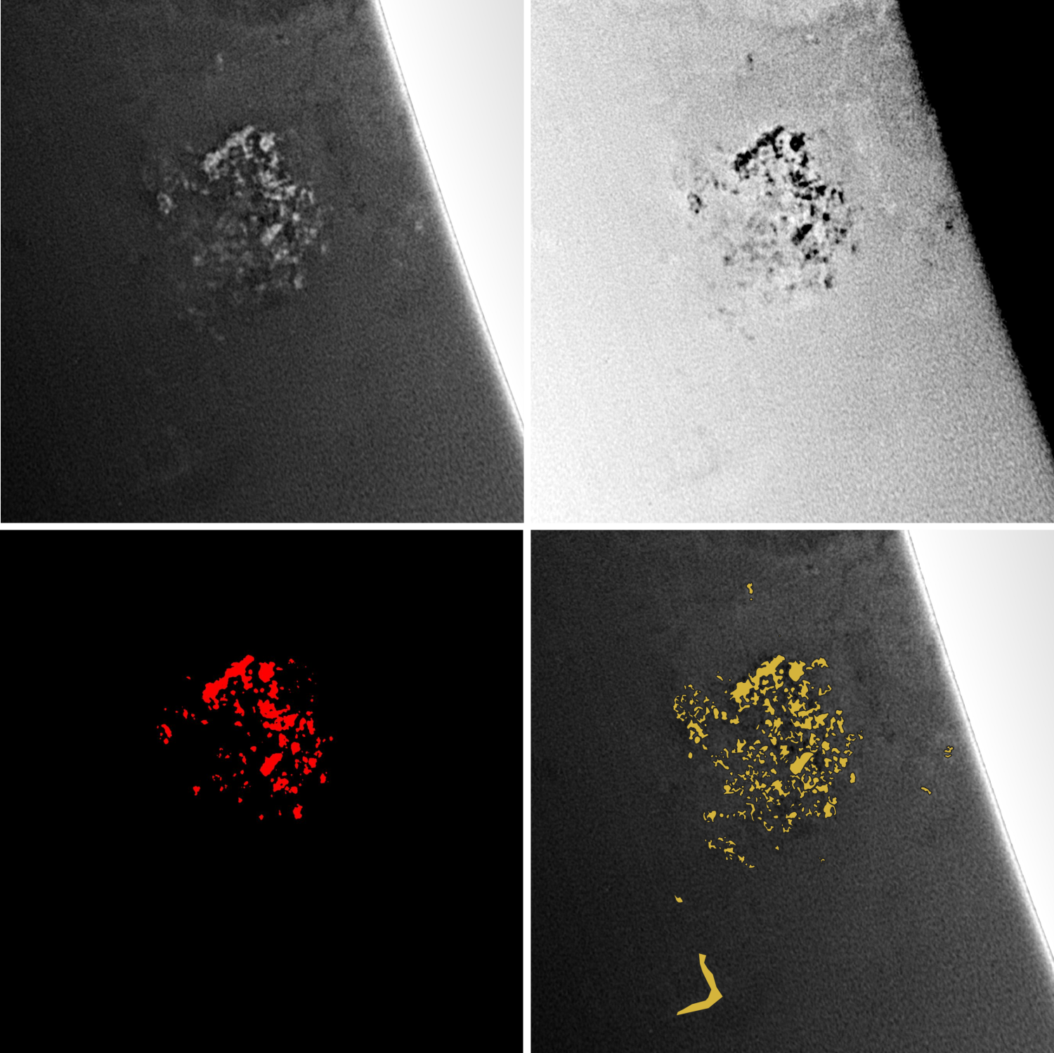
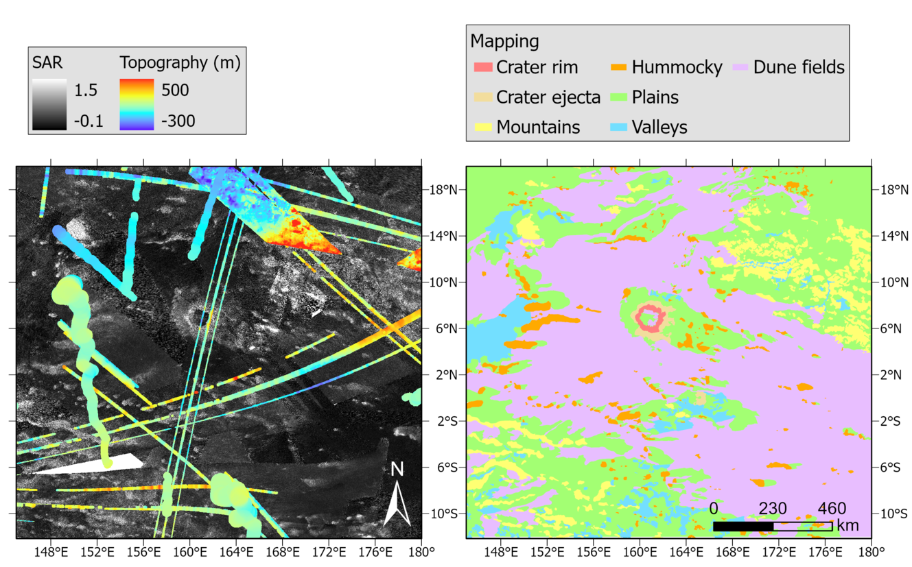
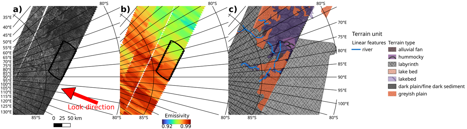
Figure 2: Cassini SAR image a), emissivity map b) and geomorphological analysis c) of a portion of the T59 RADAR swath where a RoI was identified.

In the case of T592 RoI, the vicinity of the correlation zone includes labyrinthic terrains, plains and rivers flowing into a large radar-dark region of low altitude (according to topography data) identified as a possible dry paleolake. The RoI is centred on a triangularly-shaped radar-dark feature of dimension 19x47km2, crossed by a canyon (digged by rivers) and tagged as an alluvial fan. A similar but smaller triangular dark feature can be seen on the west despite not being detected.

Comparison to a combined radar and radiometer model
Consistent with our geomorphological analysis, we propose that the correlation between e and σ° could be explained by the presence of two superimposed layers with the bottom layer having a lower permittivity and a larger roughness than the top layer. Top layer could be made of fine-grained organic sediments deposited over a rough substrate of water ice or solidified organics. Such hypothesis is supported by the two-layer radar and radiometry model we developed based on [9,10] for e and [11] for σ° (Fig. 3). Variations along the correlation slope would be simply due to variations of the thickness of the upper layer from one radar/radiometry footprint to the other.

Figure 3: a) 2-layer model displaying the roughness of the upper and lower layers and the distance between the interfaces (i.e. upper layer thickness). The top layer has a permittivity of 2+0.001j and the bottom layer of 3+0.0001j. d) Scatterplot of the simulated emissivities and σ° with the computed correlation coefficient.

Discussion and Perspectives
We have found that, among the ten RoIs detected as exhibiting a strong positive correlation between Cassini active and passive RADAR dataset, six are geomorphologically consistent with areas of sediment deposition as they exhibit features due to fluvial activity in an ancient lake system. In this paper, we will further describe these regions and how the joint analysis of active and passive radar data can serve as a tool for detecting them.

References
[1] Lopes+2020
[2] Stofan+2007
[3] Malska+2016
[4] Malaska+2020
[5] Elachi+2005
[6] Paganelli+2008
[7] Lorenz+2016
[8] Jennings+2019
[9] Le Mouelic+2008
[10] Ulaby & Long2014
[11] Le Gall+2016
[11] Hayes+2010

How to cite: Sultana, R. and Le Gall, A.: Tagging Titan's Terrains as Potential Sediment Deposits from the joint analysis of Cassini Active and Passive RADAR Observations, Europlanet Science Congress 2024, Berlin, Germany, 8–13 Sep 2024, EPSC2024-824, https://doi.org/10.5194/epsc2024-824, 2024.

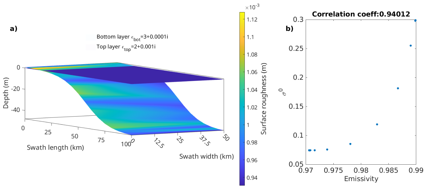
Atmosphere chemistry and hazes
14:50–15:00
|
EPSC2024-573
|
ECP
|
On-site presentation
Koyena Das, Thomas Gautier, Cyril Szopa, Sandrine Vinatier, Sarah M Hörst, Joseph Serigano, Maélie Coutelier, Jules Houbin, Bruno de Batz de Trenquelléon, and Melissa G. Trainer

Introduction

In Titan, the two major gases nitrogen (N₂) and methane (CH₄) are ionized and/or photolyzed at high altitudes by the sunlight and the energetic particles from Saturn's magnetosphere, resulting in a rich atmospheric chemistry comprising of a wide variety of carbon and nitrogen-bearing compounds (see for example Vuitton et al. 2019). These molecules combine to form heavier and more complex molecules until they become heavy enough that they are unable to retain their gaseous phase. These molecules then turn into aerosols and travel down into the atmosphere where they aggregate with other aerosols to form bigger particles, finally forming a haze layer at approximately 500 km. The simple gaseous species also travel deep into the atmosphere until they reach the tropopause, where most of them condense (Wilson and Atreya 2004). 

The Cassini Huygens mission which was launched in 1997, reached the Cronian system in mid-2004. The Huygens probe detached itself from the orbiter in December 2004 and entered Titan’s atmosphere on 14 January 2005. With the objective of studying the lower atmosphere, the science instruments started operating from an altitude of 150 km and took measurements for three hours-2.5 hrs in the atmosphere and an hour on the ground (Niemann et al 2010). In the present work, we focus on studying the vertical profiles of trace species in the lower atmosphere using the measurements by the GCMS on the probe, to obtain a better insight into the atmospheric processes taking place there. 


Methodology

The GCMS stage 2 files were used for this work. It has been corrected for detector dead time and saturation (Niemann et al. 2010). The background was also removed from the data. Finally, upon closer inspection, we find that there has been cross-contamination between mass peaks 26-29 because of mass-28 (from N₂). This was corrected by fitting lognormal curves for each unit mass peak on the fractional mass scans (least count: 0.125 amu) that were taken during the probe descent. 

The corrected mass spectra were then used as an input to a mass spectra deconvolution code developed by Gautier et al. 2020. A database of fractionation patterns of 10 species (from NIST and Cassini-INMS calibrations) was created. Our code runs 100,000 Monte Carlo simulations in which the peak intensities of each species’s fragmentation pattern are varied by a certain percentage (±30% in our case). Using a least square linear equations solver, we compute the mole fractions of each species for each simulation at every altitude. The best simulations for each species are chosen when their solutions do not lie near the predefined boundary limits. The solutions of these best simulations are then averaged to get the mole fractions at each altitude.

Results and discussions

Figure 1: Vertical profile of mole fractions of five trace species- a) acetylene, b) hydrogen cyanide, c) ethane, d) argon, and e) ethylene in their gaseous phase (plotted with their standard deviations) with a resolution of 5 km.

The vertical profiles of five trace species are shown in Figure 1. Ethane and ethylene have been plotted with their upper limits. Upon comparing these results with the computed mole fractions from CIRS (Mathe et al 2020) and the Titan PCM, it is evident that the mole fractions calculated in this work are higher than what was expected. Most trace gases condense near tropopause, so there should have been a decrease in mole fractions after that, which is not the case here. Hence we present here three hypotheses to interpret the results.

The first hypothesis claims that there might have been significant recombination inside the ion source which could have led to false detection in the spectra. A sudden change in any physical parameters inside the ion source could imply the significance of this phenomenon. However, the lack of available information makes it difficult for us to support this claim which is why we believe that maybe this process was negligible during the descent. The next hypothesis says that frost formed on the surface of the probe while it was passing the condensation region. This could have accumulated at the entrance of the probe which then evaporated by the time the instrument was operational. If any significant layer of frost deposited on Huygens, it would have induced a plateau in the temperature profile measured by the HASI, which was clearly not the case. Thus we cannot explain our results with the existence of frost, and can firmly exclude this hypothesis. Our final hypothesis states that aerosols could be evaporated at certain places inside the probe due to the high temperature inside the instrument compared to the outside. Hence the dataset would contain a mixture of evaporated aerosols and gaseous species which could explain the high mole fractions. The probability of the occurrence of this hypothesis is the strongest among the three.

To summarise, GCMS did not measure just atmospheric gases but could have also measured some aerosols and condensed particles that were trapped in the instrument. Laboratory experiments on Titan tholins are currently being done at low temperatures to investigate this possibility. 

References

Vuitton, V., Yelle, R. V., Klippenstein, S. J., Hörst, S. M., and Lavvas, P. (2019). Simulating the density of organic species in the atmosphere of Titan with a coupled ion-neutral photochemical model. Icarus, 324:120–197

Wilson, E. H. and Atreya, S. K. (2004). Current state of modeling the photochemistry of titan’s mutually dependent atmosphere and ionosphere. Journal of Geophysical Research: Planets, 109(E6)

Niemann et al. Composition of Titan’s lower atmosphere and simple surface volatiles as measured by the Cassini-Huygens probe gas chromatograph mass spectrometer experiment. JGR 115, E12006, 2010

Gautier et al. Decomposition of electron ionization mass spectra for space application using a Monte-Carlo approach. Rapid. Com. Mass Spec. 34(8), e8659 (2020)

Mathé, C., Vinatier, S., Bézard, B., Lebonnois, S., Gorius, N., Jennings, D. E., Mamoutkine, A., Guandique, E., and Vatant d’Ollone, J. (2020). Seasonal changes in the middle atmosphere of Titan from Cassini CIRS observations: Temperature and trace species abundance profiles from 2004 to 2017. Icarus, 344:113547

How to cite: Das, K., Gautier, T., Szopa, C., Vinatier, S., Hörst, S. M., Serigano, J., Coutelier, M., Houbin, J., de Batz de Trenquelléon, B., and Trainer, M. G.: Reanalysis of trace species in Titan’s lower atmosphere from Huygens GCMS, Europlanet Science Congress 2024, Berlin, Germany, 8–13 Sep 2024, EPSC2024-573, https://doi.org/10.5194/epsc2024-573, 2024.

15:00–15:10
|
EPSC2024-1063
|
On-site presentation
Nadia Balucani and Marzio Rosi

Aromaticity, a property of ring-shaped molecular structures with resonant π bonds, confers increased stability to aromatic compounds compared to other chemical arrangements of the same groups of atoms. For this reason, aromatic rings are very stable and, upon chemical attack, are expected to evolve further while retaining their aromatic nature. This is also why polycyclic aromatic hydrocarbons (PAHs) are ubiquitous in contexts where the first aromatic ring can form. 

Since the first laboratory experiments simulating the conditions of the atmosphere of Titan, polycyclic aromatic hydrocarbons (PAHs) were suggested as possible components of the haze aerosol [1]. The detection of benzene, the simplest aromatic hydrocarbon, supported this suggestion since benzene can easily evolve towards PAHs. Benzene is quite diffuse in Titan as it has been identified in the upper atmosphere (peak around 1000 km), in the mesosphere, in the stratosphere, and even on the surface upon the impact of the Huygens probe [2-5].

The presence of the N-heterocyclic aromatic molecules was also considered after the analysis of INMS spectra where ions at m/z 80 and 81, corresponding to protonated pyridine and pyrimidine or their isomers, were identified. Attempts to confirm their detection via ALMA failed and only upper limits were derived [6]. However, the analysis of an unidentified emission band near 3.28 microns observed in the upper daytime atmosphere [7] suggested a contribution from N-containing PAHs (such as N-heterocyclic compounds or aromatic amines) in addition to PAHs [8]. Furthermore, the CAPS-IBS data can be interpreted by considering that PAHs and N-containing PAHs are responsible for the heavy positive ions signal between 170–310 Da [9]. 

In conclusion, there must be active reaction mechanisms causing the incorporation of nitrogen into aromatic compounds. Since molecular nitrogen is not a reactive species, nitrogen ions or atoms must be responsible for that. Interestingly, photodissociation, dissociative photoionization, cosmic-ray-induced dissociation, electron impact as well as N2+ dissociative recombination can produce atomic nitrogen in the first electronically excited 2D state (a metastable state with a very long radiative lifetime) in similar amounts to the ground 4S state [10]. N(4S) exhibits very low reactivity with closed-shell molecules, while N(2D) is reactive also with the abundant closed-shell molecules of Titan [10].

For this reason, we have started a systematic investigation of the reactions between N(2D) and simple aromatics, like benzene itself, pyridine, and toluene. We have employed the same combined experimental and theoretical approach described in Refs. [11,12,13]. The reaction mechanism has been elucidated for the three systems and the reaction products with their relative yield have been determined [14,15]. In all cases, the ring contraction channel is the dominant one (thus confuting the dogma on the stability of the aromatic rings towards chemical attack) but, among the minor species, interesting cyclic structures incorporating N have been observed.

[1] C. Sagan, B. N. Khare, W. R. Thompson, G. D. McDonald, M. R. Wing, J. L. Bada, T. Vo-Dinh and E. T. Arakawa, Astrophys. J., 1993, 414, 399–405.

[2] J. H. Waite Jr, et al., Science, 2007, 316, 870–875.

[3]  T. T. Koskinen, R. V. Yelle, D. S. Snowden, P. Lavvas, B. R. Sandel, F. J. Capalbo,

[4] Y. Benilan and R. A. West, Icarus, 2011, 216, 507–534.

[5] H. B. Niemann, et al., Nature, 2005, 438, 779–784.

[6] C. A. Nixon, ACS Earth Space Chem., 2024,  3, 406–456.

[7] B. M. Dinelli, M. Lopez-Puertas, A. Adriani, M. L. Moriconi, B. Funke, M. Garcıa-Comas and E. D’Aversa, Geophys. Res. Lett., 2013, 40, 1489–1493.

[8] M. Lopez-Puertas, B. M. Dinelli, A. Adriani, B. Funke, M. Garcıa-Comas, M. L. Moriconi, E. D’Aversa, C. Boersma and L. J. Allamandola, Astrophys. J.,
2013, 770, 132.

[9] R. P. Haythornthwaite, A. J. Coates, G. H. Jones, A. Wellbrock, J. H. Waite, V. Vuitton and P. Lavvas, Planet. Sci. J., 2021, 2, 26.

[10] O. Dutuit, et al., Astrophys. J. Suppl. Ser., 2013, 204, 20.

[11] N. Balucani, A. Bergeat, L. Cartechini, G. G. Volpi, P. Casavecchia, D. Skouteris and M. Rosi, J. Phys. Chem. A, 2009, 113, 11138–11152.

[12] N. Balucani, D. Skouteris, F. Leonori, R. Petrucci, M. Hamberg, W. D. Geppert, P. Casavecchia and M. Rosi, J. Phys. Chem. A, 2012, 116, 10467–10479.

[13] G. Vanuzzo, D. Marchione, L. Mancini, P. Liang, G. Pannacci, P. Recio, Y. Tan, M. Rosi, D. Skouteris, P. Casavecchia and N. Balucani, J. Phys. Chem. A, 2022, 126, 6110–6123.

[14] N. Balucani, A. Caracciolo, G. Vanuzzo, D. Skouteris, M. Rosi, L. Pacifici, P. Casavecchia, K.M. Hickson, J.-C. Loison and M. Dobrijevic, Faraday Disc., 2023 245, 391-445

[15] L. Mancini, G. Vanuzzo, P. Recio, A. Caracciolo, N. Faginas-Lago, M. Rosi, P. Casavecchia, N. Balucani, J. Phys. Chem. A, submitte


How to cite: Balucani, N. and Rosi, M.: Aromatic compounds and their reactions with atomic nitrogen in the upper atmosphere of Titan, Europlanet Science Congress 2024, Berlin, Germany, 8–13 Sep 2024, EPSC2024-1063, https://doi.org/10.5194/epsc2024-1063, 2024.

15:10–15:15
15:15–15:25
|
EPSC2024-501
|
ECP
|
On-site presentation
Rafael Rianço-Silva, Pedro Machado, Zita Martins, Emmanuel Lellouch, Jean-Christophe Loison, Michel Dobrijevic, João Dias, and José Ribeiro

The atmosphere of Titan is a unique natural laboratory for the study of atmospheric evolution and photochemistry akin to that of the primitive Earth (1), with a wide array of complex molecules discovered through infrared and sub-mm spectroscopy (2) (3). Here, we present the results of the exploration of original, ground-based, very high-resolution visible spectra of Titan, obtained with VLT-UVES (4), shedding light on a poorly explored part of Titan’s spectrum – containing understudied visible methane absorption bands – with high-resolution ground-based spectroscopy. Here we also present a new, Doppler-based line detection method for backscattered planetary atmosphere spectra: By comparing VLT-UVES spectra of Titan obtained in distinct observation nights (with distinct radial velocities between Titan and the Sun) it was possible to automatically distinguish absorption lines originated on Titan’s atmosphere from backscattered solar absorption lines. This allowed to retrieve an empirical, low Temperature (T < 200K), high resolution (R = 100.000) line list of methane absorption on Titan, between 525nm and 618nm, for which no similar line lists are yet available (5), identifying and characterising more than 90 new high energy CH4 lines. Interestingly, these newly detected individual absorption lines explain previous low-resolution and low-temperature (T < 200K) profiles of visible methane absorption bands (6).

Furthermore, we searched for the predicted, but previously undetected carbon trimer molecule, C3 (7) (8), on the atmosphere of Titan, at its 405.1 nm band, by comparing VLT-UVES Titan spectra with a line-by-line (9) model spectrum of Titan’s atmosphere with C3. This understudied transient photochemical molecule is thought to play a key role on the photochemical pathways leading to the formation of aromatic organic molecules such as benzene in Titan (10). C3 abundance on Titan’s upper atmosphere could therefore be a proxy for the photochemical reaction rates that govern the production of aromatic compounds on Titan.  Our results suggest the presence of C3 at the upper atmosphere of Titan, with an estimated column density of ((1.0 ± 0.6) ×1013 cm−2), a value 5x lower than the C3 column density predicted by previous photochemical models of Titan’s high atmosphere (7)(8). This study of Titan's atmosphere with very high-resolution visible spectroscopy presents a unique opportunity to observe a planetary target with a CH4-rich atmosphere, from which CH4 optical proprieties can be studied (11). It also showcases the use of a close planetary target to test new methods for chemical retrieval of minor atmospheric compounds, in preparation for upcoming studies of cold terrestrial exoplanet atmospheres (12).

Figure 1: Line detection with the Doppler Method for Spectral line identification at a section of the 5430 Å CH4 band. By comparing distinct nightly VLT-UVES spectra of Titan (coloured spectra), corresponding to distinct radial velocities between Titan and the Sun, it is possible to distinguish between Doppler-shifted backscattered solar absorption lines (also present in at the normalized solar spectrum, in black) and “fixed” absorption lines originating from Titan’s rest frame.

Figure 2: Normalised Spectrum of Titan (black) compared with synthetic normalised spectra of Titan for several C3 column densities, N(C3), sweeping from 0 to 2,0 × 1013 cm−2, with steps of 4,0 × 1012 cm−2. Vertical grey lines correspond to C3 line centres and respective uncertainty (9). Red ellipses evidence three possible detections of absorption lines in Titan spectrum that are not explained by backscattered of solar radiation alone — but instead match the expected wavelengths of C3 absorption lines.

References: (1) Hörst S., 2017; J. Geophys. Res. Planets, doi:10.1002/2016JE005240; (2) Nixon C., et al, 2020; The Astronomical Journal, doi:10.3847/1538-603881/abb679; (3) Lombardo N., et al, 2019, The Astrophysical Journal Letters, 2019 doi:10.3847/2041658213/ab3860; (4) Rianço-Silva R., et al, 2024, Planetary and Space Sciences, 240, 105836, https://doi.org/10.1016/j.pss.2023.105836. (5) Hargreaves R., et al, 2020; The Astrophysical Journal Supplement Series, doi:10.3847/1538-4365/ab7a1a; (6) Smith, W.H., et al., 1990, Icarus, 85; (7) Hérbad E., et al, 2013; Astronomy & Astrophysics, doi:10.1051/0004-6361/201220686; (8) Dobrijevic M., et al, 2016; Icarus, doi.org/10.1016/- j.icarus.2015.12.045; (9) Schmidt M., et al, 2014; MNRAS, doi.org/10.1093/mnras/stu641; (10) Loison, J. et al, 2019, Icarus, 329; (11) Thompson M., et al, 2022; PNAS, doi.org/10.1073/pnas.2117933119; (12) Tinetti G., et al, 2018; Experimental Astronomy, doi:10.1007/s10686-018-9598-x


How to cite: Rianço-Silva, R., Machado, P., Martins, Z., Lellouch, E., Loison, J.-C., Dobrijevic, M., Dias, J., and Ribeiro, J.: A study of very high resolution visible spectra of Titan - Caracterization of visible CH4 bands and the search for C3, Europlanet Science Congress 2024, Berlin, Germany, 8–13 Sep 2024, EPSC2024-501, https://doi.org/10.5194/epsc2024-501, 2024.

15:25–15:35
|
EPSC2024-670
|
On-site presentation
Conor Nixon, Bruno Bezard, Thomas Cornet, Brandon Coy, Imke de Pater, Maël Es-Sayeh, Heidi Hammel, Bryan Holler, Emmanuel Lellouch, Nicholas Lombardo, Manuel López-Puertas, Juan Lora, Stefanie Milam, Pascal Rannou, Sébastien Rodriguez, Nicholas Teanby, and Elizabeth Turtle

Saturn’s moon Titan is the only moon in the solar system with a dense atmosphere, composed largely of nitrogen (94.5–98.6%) and methane (5.5–1.4%). Due to the cold troposphere and surface (70–93 K) close to the triple point of methane, methane is a condensable substance in Titan’s lower atmosphere. It therefore plays a similar meteorological role to water on Earth, evaporating from the surface and reaching the middle troposphere, where methane clouds form and rainfall occurs, in changing seasonal patterns. In the middle and upper atmosphere, methane is processed by photochemistry and at high altitudes forms solid organic haze particles or even PAHs (polycyclic aromatic hydrocarbons). These particles are thought to be the building blocks of stratospheric aerosols as they drift downwards and grow in size to form a global haze layer in the stratosphere, which lends Titan its golden hue at visible wavelengths. In the stratosphere, slow seasonal changes in composition and haze distribution indicate the seasonal reversal of Titan’s global meridional circulation every 14.75 Earth years.

Since the end of the Cassini-Huygens mission in September 2017 our ability to monitor Titan’s changing atmosphere has been curtailed, since we have lacked the ability to view Titan unimpeded by the Earth’s atmosphere across all infrared wavelengths. Nevertheless, using ground-based adaptive optics (AO) imaging from the Keck observatory on Maunakea, cloud monitoring was possible, although only in some near infrared (NIR) spectral windows. With the commissioning of the James Webb Space Telescope (JWST) in 2022 it became possible to view Titan once more at wavelengths from ∼1.0 to 28.0 μm.

In this article we report results of JWST imaging and spectroscopy of Titan that occurred in November 2022 and July 2023, using three of the four observatory instruments. We also report on contemporaneous ground-based observations with the Keck NIRC2 camera that provided even higher spatial resolution imaging over a wider time range, but in a more limited set of filters. Imaging data from JWST and Keck reveals clouds at mid and high northern latitudes at different altitudes, suggestive of convection at the latitudes of the northern lakes and seas. Spectroscopy with JWST/NIRSpec enabled the detection of the CO2 4.3-μm bands and measurement of the detailed structure of the CO 4.7-μm non-LTE emission. Finally, with JWST/MIRI we made the first detection of the CH3 radical, opening new views into the photochemistry occurring in the upper atmosphere.

Together, these results provide new insights into the changes in the composition and meteorology of Titan’s atmosphere that have occurred since the end of Cassini-Huygens in 2017, as Titan’s late northern summer ebbs towards the upcoming fall equinox in 2025.

Figure 1: JWST (July 11th) and Keck (July 8th and 14th) observations of Titan. Upper row: RGB color composite images. JWST:  blue=1.4 mm, green=1.5 mm, blue=2.0 mm (filters F140M, F150W, and F200W, respectively. Keck: blue=2.13 mm, green=2.12 red=2.06 mm (H2 1-0, Kp, and He1b, respectively). Second row: single-wavelength images taken by JWST and Keck at 2.12 mm sensitive to emission from Titan’s lower troposphere. Third row: emission at 1.64 mm (JWST) and 2.17 mm (Keck) sensitive to Titan’s upper troposphere and stratosphere. Fourth row: Titan orientation on the sky as seen on the different dates. Clouds are seen at higher altitudes on July 14th than earlier on July 8th and 11th, suggesting upward convection.


How to cite: Nixon, C., Bezard, B., Cornet, T., Coy, B., de Pater, I., Es-Sayeh, M., Hammel, H., Holler, B., Lellouch, E., Lombardo, N., López-Puertas, M., Lora, J., Milam, S., Rannou, P., Rodriguez, S., Teanby, N., and Turtle, E.: Titan’s Atmosphere in Late Northern Summer from JWST and Keck Observations, Europlanet Science Congress 2024, Berlin, Germany, 8–13 Sep 2024, EPSC2024-670, https://doi.org/10.5194/epsc2024-670, 2024.

15:35–15:45
|
EPSC2024-412
|
On-site presentation
Pascal Rannou, Bruno Bézard, Emmanuel Lellouch, Sébastien Rodriguez, Maël Es-Sayeh, Robert West, Bruno de Batz de Trenquelléon, and Conor Nixon

 The photochemical haze layer in the stratosphere above about 80 km and the condensation haze (hereafter, mist) in the lower stratosphere and troposphere completely cover Titan and play a dominant role in its climate. These hazes determine the atmospheric radiative balance and are also good tracers of the atmospheric circulation. Spatial and temporal characterization of the haze is therefore essential for understanding Titan's climate. It is also an important step towards accessing surface properties and cloud characteristics. Recently, the James Webb Space Telescope (JWST) has provided observations of very high spectral quality. These images and spectra provide information on the latitudinal distribution of haze, from the lower stratosphere (100-150 km) down into the troposphere with good vertical resolution. With this dataset, we are able to describe the mist layer in five distinct sublayers : the deepest layer between 0 and 40 km and four layers of 10 km thickness between 40 and 80 km. The retrievals performed allow us to reconstruct a map of the haze and mist layer on the date of observation (5 November 2022) and thus highlight haze distributions related to circulation. For this analysis, we used a plane-parallel model and thus we are restricted to latitudes between -30°S and 60°N. In details, we found a photochemical haze layer increasing from the north to the south, as expected. Below 80 km, the mist layers have a more complex distribution. The deepest layer (below 40 km) has an opacity minimum near the equator and increasing toward both poles. The opacity of the mist layer between 40 and 80 km gradually changes, from bottom to top, to reach a monotonously increasing opacity from the south to the north, as for the stratospheric haze. In all bands, we find a marked opacity feature above 50 km, south to 10°S, that form a detached mist layer slightly emerging from the background opacity. We could also retrieve the surface reflectivity, with a quite low spatial resolution, that will also be discussed. With the same model, we also analyzed a selected part of the huge VIMS/Cassini data set. We could monitored, albeit with a lower vertical resolution, how these hazes evolve over the season. Here the mist layer is described in only three distinct layers but the observation set spans from 2004 to 2017. During Cassini era, we probe the seasonal change of the haze and the mist layer and have a view on the seasonal modulation of all the layers. These results allow for putting in context the results obtain with the JWST. Moreover, it also offers an interesting comparison for the results obtained with JWST since Cassini observed the opposite season, in 2007. Finally, we can fully understand our results with the help of the Titan Planetary Climate Model (PCM), now coupled with haze and cloud microphysics. This model predicts the evolution of the haze and the mist within the seasonal cycle. The haze layer is transported by dynamics and its distribution is fairly straightforward to understand. The mist, in addition, is also controlled by thermodynamical conditions which must be modeled in detail to be predicted. Then, the mist layers, less opaque in the equatorial region and increasing toward the mid-latitudes and the detached mist layer found with the JSWT are described by the PCM and correlated to the hadley-type cell below 80 km and to the temperature latitude profile. Figure 1 shows the haze and mist layers retrieved in our work. Over the JWST lifetime, we hope to complete the seasonal survey of atmospheric properties for the upcoming period from the northern autumn equinox to the winter solstice. This is a poorly observed period but corresponds to a complete reversal of atmospheric circulation. Significant changes are expected to be observed during this period. With the upcoming very large telescopes (EELT, TMT, etc.) with high sensitivity and spectral resolution, this work shows that an increase in spectral resolution translates - up to a certain point - into an increase in vertical resolution. Finally, the complete characterization of haze and cloud cycles, with models and constraints from the most precise observations possible, is a major objective to prepare for future missions to Titan; Dragonfly but also those which may be decided upon in the near or distant future.

Figure 1 : Haze and mist extinction retrieved with the NIRSpec/JWST (5 Nov 2022) (top) and with VIMS/Cassini (2007) (bottom) at 2 μm. The sub-solar latitude was in the northern hemisphere (12.62°N) at the JWST observation date and in the southern hemisphere (between 14.25°S and 8.90°S) during the year 2007.


How to cite: Rannou, P., Bézard, B., Lellouch, E., Rodriguez, S., Es-Sayeh, M., West, R., de Batz de Trenquelléon, B., and Nixon, C.: Titan haze and mist layers observed by Nirpsec/JWST and comparison with inversions from VIMS/Cassini and Planetary Climate Model of Titan., Europlanet Science Congress 2024, Berlin, Germany, 8–13 Sep 2024, EPSC2024-412, https://doi.org/10.5194/epsc2024-412, 2024.

15:45–15:55
|
EPSC2024-177
|
ECP
|
On-site presentation
Zili He, Sandrine Vinatier, Vincent Eymet, Vincent Forest, Bruno Bezard, Pascal Rannou, Sébastien Rodriguez, Emmanuel Marcq, Richard Fournier, Stéphane Blanco, Nada Mourtaday, Yaniss Nyffenegger-Pere, Sébastien Lebonnois, and Anni Määttänen

The Cassini mission has gathered extensive near-infrared spectra and imagery of Titan, which pose challenges for analysis due to the significant scattering effects of its atmosphere with potential heterogeneous radiative properties. Traditional radiative transfer models used to analyze Cassini data often employ plane-parallel or pseudo-spherical approximations and assume that atmospheric layers are horizontally uniform. To address these limitations, a new radiative transfer code that solves a spherical and heterogeneous model based on the Monte Carlo method has been developed [1].

 This new radiative transfer solver takes into account the geometry of a "ground" of arbitrary shape, described by a triangular mesh, with the possibility of using an arbitrary number of materials. The radiative properties of a gas mixture are provided on a tetrahedral mesh using the k-distribution spectral model. The radiative properties of an arbitrary number of aerosols and clouds can also be provided on their individual meshes.

 Furthermore, to retrieve atmospheric (e.g., haze density, top of cloud altitude, etc.) or surface properties, not only the intensity but also its gradient (the so-called sensitivities) are needed. Since these gradient calculations cannot be done with finite differences with the Monte Carlo approach, we need to differentiate the Monte Carlo estimator of intensity to build the Monte Carlo estimator of sensitivities. By conserving the same random paths for the estimation of intensity and all sensitivities, the extra calculation time to estimate all these quantities is minimized. A vectorized Monte Carlo estimator is then built, which can estimate simultaneously the intensity and its gradient. Currently, the estimation of sensitivities of mixed gas radiative properties is not available because of its complexity, which needs further development.

 The methodology is applied to Titan's atmosphere, where we perform sensitivity analysis. The results show that because of the strong scattering effect in the atmosphere, the heterogeneity of the surface and atmosphere impacts a lot of the observable (i.e., the measured intensity), which cannot be investigated by classical parallel-plane and homogeneous layers radiative transfer solvers. For instance, we show that at around 933 nm, the surface reflectivity at 250 km away from the targeting point still has an unnegligible effect on the measured signal. Similarly, sensitivity analysis is also performed on the aerosol density in the atmosphere. These sensitivity analyses help understand the scattering effect in Titan's atmosphere and help design the inversion process of atmospheric properties. This project was funded by French National Research Agency (ANR-21-CE49-0020).

[1] htrdr, Meso-Star https://www.meso-star.com/projects/htrdr/htrdr.html


How to cite: He, Z., Vinatier, S., Eymet, V., Forest, V., Bezard, B., Rannou, P., Rodriguez, S., Marcq, E., Fournier, R., Blanco, S., Mourtaday, N., Nyffenegger-Pere, Y., Lebonnois, S., and Määttänen, A.: A spherical and heterogeneous radiative transfer code for near-infrared remote sensing: application to Titan, Europlanet Science Congress 2024, Berlin, Germany, 8–13 Sep 2024, EPSC2024-177, https://doi.org/10.5194/epsc2024-177, 2024.

15:55–16:00
Coffee break
Chairpersons: Audrey Chatain, Thomas Gautier
Methane cycle and clouds
16:30–16:40
|
EPSC2024-735
|
On-site presentation
Daniel Cordier, Zhen Wang, Benoît Seignovert, and Robert A. West

Titan, the enigmatic large moon of Saturn, is the unique satellite of the solar system surrounded by a dense atmosphere which has a significant effect on radiation polarization. The Cassini exploration of the kronian system has also revealed the existence of large bodies of liquid at the surface of Titan. It is well known that smooth surfaces polarize the reflected electromagnetic waves, that aspect reinforces the interest of a polarimetric study of the Saturn main satellite. On board the Cassini probe, the ISS (Imaging Science Subsystem) instrument was equipped with a large set of spectral and polarized filters that could be combined with one another.

By using near infrared filters together with polarized filters, we have searched for features highlighted by polarimetric observations, we have targeted both the surface and the atmosphere. We first worked at the near-infrared wavelength of 939 nm, at which the atmosphere of Titan is slightly transparent. The spectral filter CB3 is then employed with two polarization filters, with perpendicular direction. The resulting polarization maps are interpreted with the help of a multidimensional Monte-Carlo radiative transfer model specifically adapted to Titan’s atmosphere.


How to cite: Cordier, D., Wang, Z., Seignovert, B., and West, R. A.: Titan's elusive clouds seen in polarization, Europlanet Science Congress 2024, Berlin, Germany, 8–13 Sep 2024, EPSC2024-735, https://doi.org/10.5194/epsc2024-735, 2024.

16:40–16:55
|
EPSC2024-845
|
ECP
|
On-site presentation
Bruno de Batz de Trenquelléon, Pascal Rannou, Sébastien Lebonnois, and Jérémie Burgalat

1. Principle of the work

    On Titan, as on Earth, a wide variety of clouds form from various processes and conditions. Unlike our planet, clouds on Titan emerge from a variety of volatile compounds. Observations have shown several types of cloud, such as convective clouds of methane, stratiform clouds of ethane, or high-altitude clouds containing compounds like HCN and HC3N. In addition, a large high-altitude HCN ice cloud was discovered in May 2012, formed in the polar vortex at the South Pole [1]. Generally, convective methane clouds are found at the summer pole and mid-latitudes, while other types of cloud are observed at the winter pole. Despite the various observations made by Cassini and Huygens between 2004 and 2017, we still have a limited understanding of the couplings between the different cycles that take place on Titan (haze, clouds, gas, etc.).
    
    The Titan Planetary Climate Model (Titan PCM), first developed at the Institut Pierre-Simon Laplace, is the ideal tool for understanding how these cycles work and how clouds form on Titan. The transition of the model into three dimensions has considerably improved our knowledge of the mechanisms of Titan's middle atmosphere [2]. The microphysical processes associated with haze were implemented in the Titan PCM a long time ago, and we now have adapted and implemented a microphysical model to simulate the processes associated with clouds of CH4, C2H2, C2H6 and HCN [3]. We plan to include convective aspects in forthcoming studies. These are phenomena that have not yet been simulated in Titan's 3D climate models, in particular the nucleation and condensation of methane clouds, which are responsible for much of Titan's cloud cover.


2. Results & Discussion

    In this presentation, we propose to use a microphysical cloud model, integrated into the Titan PCM, to study the formation and evolution of hydrocarbon clouds throughout the Titanian year. We will analyse the thermal structure of the model, enabling the formation of the HCN cloud observed at around 300 km. Particular attention will be focused to the methane cycle, including its sources, sinks and associated processes. We will also look at the microphysical properties of the clouds and the constraints on the parameters influencing their formation. The results of the model (Figure 1) will then be compared with existing observations.

Fig. 1 Zonal average of the clouds extinction at 0.7 μm at the South Pole. The extinction above 100 km corresponds to clouds of HCN, while the extinction below is associated with C2H2 and C2H6 clouds. Peaks of extinction between 10 km and 20 km correspond to CH4 clouds. The altitude scale on the right axis is approximate.


This project is in line with previous research aimed at providing answers to persistent questions and deepen our understanding of Titan's atmosphere. The model will be used to interpret future observations of the JWST, as well as preparing for the future Dragonfly mission, by better characterising the expected climate in its landing region.


3. References

[1] R. de Kok, N. Teanby, L. Maltagliati, P. Irwin, and S. Vinatier, “HCN ice inTitan’s high-altitude southern polar cloud,” , vol. 514, no.7520, pp. 65–67, 2014.

[2] S. Lebonnois, J. Burgalat, P. Rannou, and B. Charnay, “Titan global climate model: Anew 3-dimensional version of the IPSL Titan GCM,” ,vol. 218, pp. 707–722, 2012.

[3] J. Burgalat, P. Rannou, T. Cours, and E. D. Rivière, “Modeling cloud microphysics using a two-moments hy-brid bulk/bin scheme for use in Titan’s climate models:Application to the annual and diurnal cycles,” , vol. 231,pp. 310–322, 2014.

How to cite: de Batz de Trenquelléon, B., Rannou, P., Lebonnois, S., and Burgalat, J.: Microphysics of Titan's clouds: constraints on their structure, formation and transport., Europlanet Science Congress 2024, Berlin, Germany, 8–13 Sep 2024, EPSC2024-845, https://doi.org/10.5194/epsc2024-845, 2024.

16:55–17:05
|
EPSC2024-523
|
ECP
|
On-site presentation
Enora Moisan, Audrey Chatain, Aymeric Spiga, Scot Rafkin, Alejandro Soto, and Ricardo Hueso

        Titan’s methane cycle is similar to the Earth’s water cycle in many ways. Liquid methane is stable at Titan’s surface, where the pressure is around 1.5 atm and the temperature around 94 K. Methane evaporates from the methane lakes and seas, and condensates in the troposphere, forming clouds and precipitations. Contrary to Earth, where water vapor is a trace gas, methane amounts for ≈5% of Titan’s atmosphere (Niemann et al. 2010). However, clouds seem to be less abundant there than on our planet, covering around 1% of the moon while clouds cover around 60% of Earth’s surface. Our knowledge on Titan’s surface and clouds mostly comes from the Cassini-Huygens mission (2004-2017), which collected a huge amount of data, including many images, and a sounding profile through the atmosphere. While awaiting for the next in situ mission to Titan (Dragonfly, NASA, to be launched in 2028), models are a necessary tool to continue to explore the mysteries of Titan’s methane cycle.
        Modeling the methane cycle has already been performed at several scales: at planetary level, with global circulation models (e.g. Lora et al. 2019); at regional and local scales to study the local dynamics (e.g. Chatain et al. 2024), and at clouds scale. Methane convective clouds have been modeled in 2D (e.g. Barth and Rafkin 2010), and a methane thunderstorm has been reproduced in 3D (Hueso and Sánchez-Lavega 2006). Nevertheless, many questions remain. Here we focus on regional scales: on lakes and on clouds. How are lakes included in the methane cycle? What is the impact of lake morphology and of the surface properties around them? How do storm clouds form in the troposphere? How do they sometimes become global storms? How much rain do they produce, and how often?

        To tackle these questions, we first used a regional model called mtWRF (Rafkin and Soto 2020), and we studied the effects of changing the surface properties around a lake, namely the roughness, emissivity, albedo and thermal inertia (Moisan et al, in rev.). We find that these surface properties only have a minor impact on the atmospheric circulation created by the lake. Indeed, the shape of the atmospheric circulation seems to always remain the same: a thermally direct circulation, with a breeze flowing from the lake to the land at the surface. Adding topography does not change the global shape of the lake breeze either, but it creates a deeper moist layer above the lake, and increases the injection of methane in the atmosphere (see Figure 1). One of the main perspectives of this study will be to add wetlands around the lake, as land is expected to be soaked with methane there.

Figure 1: Adding topography around a lake causes the accumulation of methane vapor above the lake, and increases the altitude of methane injection in the atmosphere.

        In our regional model around a lake, the condensation of methane in the atmosphere is not allowed, thus clouds cannot form. Moreover, we do not observe saturation conditions, which could be reached higher in altitude for instance, or at other seasons. To study cloud formation, we develop a convection resolving model, coupling a dynamical core based on a modified version of WRF with physical schemes deriving from those developed for the global circulation model Titan PCM (de Batz de Trenquelléon et al. 2023). In these physical schemes the microphysics of haze and clouds is implemented, enabling the formation of clouds and precipitations. We aim to better understand the structure and formation mechanism of clouds, and to compare the model results to Cassini images. To do this, we perform new analyses of Cassini/ISS (Imaging Science Subsystem) images, with the objective to analyze cloud shapes, and to quantify cloud dynamics and lifetimes. Figure 2 shows an example where a Cassini/ISS image is used to automatically detect clouds in an image.

Figure 2: Example of automatic cloud detection with Cassini/ISS images (image N1467450031 2, taken at the very beginning of the Cassini mission, on 2004/07/02). Top left is the processed image with usual processing. Top right is the same image, but processed to make automatic cloud detection easier. Bottom left is the result of the automatic detection, while bottom right is a manual cloud selection.

References

Barth, Erika L. and Scot C. R. Rafkin (Apr. 1, 2010). “Convective Cloud Heights as a Diagnostic for Methane Environment on Titan”. In: Icarus. Cassini at Saturn 206.2, pp. 467–484. issn: 0019-1035. doi: 10.1016/j. icarus.2009.01.032. url: https://www.sciencedirect.com/science/article/pii/S0019103509000591 (visited on 09/20/2023).

Chatain, Audrey et al. (Mar. 15, 2024). “The Impact of Lake Shape and Size on Lake Breezes and Air-Lake Exchanges on Titan”. In: Icarus 411, p. 115925. issn: 0019-1035. doi: 10.1016/j.icarus.2023.115925. url: https://www.sciencedirect.com/science/article/pii/S0019103523005043 (visited on 01/03/2024).

De Batz de Trenquelléon, Bruno et al. (Oct. 1, 2023). “Simulated Methane Clouds in the Titan Troposphere with the Titan PCM”. In: 55, p. 208.07D. url: https://ui.adsabs.harvard.edu/abs/2023DPS....5520807D (visited on 05/10/2024).

Hueso, R. and A. Sánchez-Lavega (July 2006). “Methane Storms on Saturn’s Moon Titan”. In: Nature 442.7101 (7101), pp. 428–431. issn: 1476-4687. doi: 10.1038/nature04933. url: https://www.nature.com/articles/ nature04933 (visited on 09/20/2023).

Lora, Juan M. et al. (Nov. 15, 2019). “A Model Intercomparison of Titan’s Climate and Low-Latitude Environment”. In: Icarus 333, pp. 113–126. issn: 0019-1035. doi: 10.1016/j.icarus.2019.05.031. url: https://www. sciencedirect.com/science/article/pii/S0019103518307838 (visited on 01/15/2024).

Niemann, H. B. et al. (2010). “Composition of Titan’s Lower Atmosphere and Simple Surface Volatiles as Measured by the Cassini-Huygens Probe Gas Chromatograph Mass Spectrometer Experiment”. In: Journal of Geophysical Research: Planets 115.E12. issn: 2156-2202. doi: 10.1029/2010JE003659. url: https://onlinelibrary. wiley.com/doi/abs/10.1029/2010JE003659 (visited on 04/09/2024).

Rafkin, Scot C. R. and Alejandro Soto (Nov. 15, 2020). “Air-Sea Interactions on Titan: Lake Evaporation, Atmospheric Circulation, and Cloud Formation”. In: Icarus 351, p. 113903. issn: 0019-1035. doi: 10.1016/j.icarus. 2020.113903. url: https://www.sciencedirect.com/science/article/pii/S0019103520302827 (visited on 11/02/2023).

How to cite: Moisan, E., Chatain, A., Spiga, A., Rafkin, S., Soto, A., and Hueso, R.: Titan’s methane: from lakes to clouds, Europlanet Science Congress 2024, Berlin, Germany, 8–13 Sep 2024, EPSC2024-523, https://doi.org/10.5194/epsc2024-523, 2024.

17:05–17:10
Dragonfly preparation
17:10–17:20
|
EPSC2024-408
|
ECP
|
On-site presentation
Maxence Lefevre, Léa Bonnefoy, and Aymeric spiga

1. Introduction
Titan’s weather is particularly active at all spatial scales: global (e.g., super-rotating winds), intermediate / mesoscale (e.g., convective thunderstorms, air-sea circulations), local (e.g., turbulence in the planetary boundary layer, the atmospheric layer in direct contact with the surface). The aeolian environment of Titan is active, with a fifth of Titan’s surface being covered by dunes fields and the organic dust particles at the surface being potentially transported by wind circulations at all scales.
In 2034 NASA’s Dragonfly quadcopter will land and explore Selk impact crater structure in the dark Shangri-La region [1]. This area is characterized by a surface rich in organic dust particles organized as dune fields, whose peculiar morphology probably involves two distinct wind regimes that remain to be understood [2].

2. Model
To study the near-surface dynamics, a new model was developed based on the Weather-Research Forecast (WRF) non-hydrostatic dynamical core [3] and coupled with the LMD Titan PCM physics package [4]. The domain of interest is centered on Selk crater and Shangri-La region. The horizontal resolution is set to 5 km. High-resolution topography and surface characteristic such as albedo, thermal inertia and surface roughness, were created based on Cassini SAR images. The detail of these synthetic maps are described in detail in the poster presented in this session by Bonnefoy et al. The meteorological fields initial states are taken from LMD Titan PCM outputs. The mesoscale boundary conditions are forced with the LMD Titan GCM.

3. Results
Fig 1 shows Snapshots map of horizontal winds 10 m above local surface (m/s) at noon. The topography, plains and mountains, affects the direction of the surface winds. The vast majority of the wind is between ± 0.5 m/s, consistent with observations. The high mountains are able to engender mountain waves, with horizontal wind reaching 1.0 m/s. The diurnal cycle has an impact on the amplitude and direction of wind, with preferably anabatic winds during the day and katabatic winds at night. The albedo, thermal inertia and surface roughness are set constant respectively to 0.2, 335 J K−1 m−3 and 5 cm. The impact of the spatial variability due to terrain type of these parameters on the winds will be discussed.

Figure 1: Snapshots map of horizontal winds 10 m above local surface (m s−1 ) at noon in the center of the domain. The red circle represent the landing site of Dragonfly [1].

References
[1] Lorenz, R. D. et al. Selection and Characteristics of the Dragonfly Landing Site near Selk Crater, Titan. Planet. Sci. J. 2, 24 (2021).
[2] Malaska, M. J. et al. Geomorphological map of the Afekan Crater region, Titan: Terrain relationships in the equatorial and mid-latitude regions. Icarus 270, 130–161 (2016).
[3] Skamarock, W. C. & Klemp, J. B. A time-split nonhydrostatic atmospheric model for weather research and forecasting applications. Journal of Computational Physics 227, 3465–3485 (2008).
[4] Lebonnois, S., Burgalat, J., Rannou, P. & Charnay, B. Titan global climate model: A new 3-dimensional version of the IPSL Titan GCM. Icarus 218, 707–722 (2012).

How to cite: Lefevre, M., Bonnefoy, L., and spiga, A.: Mesoscale Modelling of Titan’s Shangri-La region, Europlanet Science Congress 2024, Berlin, Germany, 8–13 Sep 2024, EPSC2024-408, https://doi.org/10.5194/epsc2024-408, 2024.

17:20–17:30
|
EPSC2024-624
|
On-site presentation
Scot Rafkin, Alejandro Soto, and Guillermo Chin-Canche

Summary: The structure and evolution of Titan’s planetary boundary layer (PBL) are investigated through large eddy simulation (LES) modeling.  The PBL is the interface between the surface and the free atmosphere through which energy, mass, and momentum are exchanged.  Results from LES studies forced by diurnally-varying radiation are presented.  The development of three distinct PBL layers are noted: 1) a near-surface layer dominated by frictional dissipation; 2) a mixed-layer of near neutral stability; and 3) an entrainment layer capping the top of the PBL.  The three layers are similar in character to what is often observed in the Earth’s convective PBL. The depth and evolution of these layers is strongly affected by the initial thermal conditions, the surface thermophysical properties, and soil moisture.

Background and Motivation:  The PBL is the lowest atmospheric layer and is critical to the exchange of mass, momentum, and energy between the surface and the atmosphere. Thus, the structure, evolution, and dynamics of Titan’s PBL is relevant to understanding numerous physical processes on Titan, including but not limited to:

  • Volatile evaporation from damp regolith and lakes, and contributions to the global volatile cycle;
  • Dunes and other aeolian formations, and waves upon lakes driven by turbulent surface wind stress;
  • Conversion of surface insolation to atmospheric heating through turbulent fluxes;

In addition, missions that descend through and operate on the surface or in the atmosphere have in interest in predictions of the turbulent structure and evolution of the PBL in both the horizontal and vertical.  These predictions are relevant to the engineering design and operational planning of Dragonfly, and the predictions can be largely verified through the measurements that will be made by Dragonfly when it explores Titan.

The sounding from the Huygens probe provides the only direct, vertically resolved measurement of the structure of the PBL at a single moment in time. How the observed structures develop and evolve remain uncertain, and the turbulent exchange processes are challenging to constrain from the single profile. LES techniques provide a mechanism for understanding the observed structure and dynamics of the PBL.

Methodology: The PBL structure and evolution are investigated through LES using a version of the mesoscale Titan Weather, Research, and Forecasting (mtWRF) model (Rafkin and Soto, 2020). mtWRF has been undergoing rapid development with the addition of radiative transfer (Chatain et al., 2022), topography (Moisan et al., 2024), and realistic 3-D lake geometries (Chatain et al., 2024). In this study, we add the capability for soil moisture and prognostic latent heat fluxes and we configure mtWRF with LES grid spacing of 10 to 40 m.  The baseline simulation uses a dry regolith (no latent heat flux). Simulations with the addition of a moist surface are compared against the dry scenario. Since LES of Titan is a mostly unexplored area of research, the simulations are conducted in 2-D in order to speed analysis and discovery.  The simulations will be extended to 3-D once the PBL dynamics are better understood in 2-D.

The model is homogeneously initialized with a Huygens HASI sounding (Fulchignoni et al., 2002) over a vertical domain of 6 km and a horizontal domain of 40 km with 20 m spacing.  Starting at ~0945 local time (LT) when the HASI sounding is valid, the model is integrated until sunrise the following day.  Restarting from that point, the model is integrated again until sunset and the results of the daytime PBL evolution are analyzed.

Results: In the baseline, dry regolith case, the daytime boundary layer grows to a depth of ~1 km.  The lowest ~100 m are slightly superadiabatic with the bulk of the PBL showing a near neutral profile (Fig. 1). The top of the PBL exhibits an entrainment layer where the free atmosphere above the PBL is mixed downward. 

The peak eddy heat flux is found just above the shallow superadiabatic layer and then decreases rapidly toward zero (Fig. 1). Narrow, thermally buoyant plumes with perturbations of ~0.1 K over ambient  are evident (Fig. 2). The maximum variance near the surface is explained by the plumes that originate in this layer.  The maximum aloft is the result of gravity waves triggered by the convection below and which are trapped in the stable region at 1 km.  The subgrid-scale turbulent kinetic energy (TKE) is similar to the thermal perturbations but shows a maximum value in the near-surface layer with a secondary maximum in the middle of the PBL (Fig. 3).  The 1 km level has yet another local maximum of TKE, but is subdued compared to the thermal variance (Fig. 2).  

References:

Chatain, A., Rafkin, S.C., Soto, A. and Hueso, R., 2022, March. Mesoscale climate modeling above a methane lake on Titan. In Lunar and Planetary Science Conference.

Chatain, A., Rafkin, S.C., Soto, A., Moisan, E., Lora, J.M., Le Gall, A., Hueso, R. and Spiga, A., 2024. The impact of lake shape and size on lake breezes and air-lake exchanges on Titan. Icarus411, p.115925.

Fulchignoni, M., Ferri, F., Angrilli, F., Bar-Nun, A., Barucci, M.A., Bianchini, G., Borucki, W., Coradini, M., Coustenis, A., Falkner, P. and Flamini, E., 2002. The characterisation of Titan's atmospheric physical properties by the Huygens Atmospheric Structure Instrument (HASI). Space Science Reviews104.

Moisan, E., A. Chatain, A. Spiga, S. Rafkin, A. Soto, and R. Hueso, 2024. Titan’s methane: from lakes to clouds. EPSC 2024.

Rafkin, S.C. and Soto, A., 2020. Air-sea interactions on Titan: Lake evaporation, atmospheric circulation, and cloud formation. Icarus351.


How to cite: Rafkin, S., Soto, A., and Chin-Canche, G.: The Structure and Evolution of Titan’s Daytime Planetary Boundary Layer, Europlanet Science Congress 2024, Berlin, Germany, 8–13 Sep 2024, EPSC2024-624, https://doi.org/10.5194/epsc2024-624, 2024.

17:30–17:40
|
EPSC2024-186
|
ECP
|
On-site presentation
Paul Lagouanelle and Alice Le Gall

I.Introduction

Several lines of evidence suggest the presence of an internal global ocean on Titan [1, 2]. Among them, is the detection of a Schumann-like resonance (SR) by the Permittivity, Wave and Altimetry (PWA) analyzer on board the Huygens’ probe [3]. SR are a set of extremely low frequency electromagnetic propagation modes in a planetary cavity [4]. On Earth these modes are generated by lightning discharges and propagating between the Earth’s surface and the ionosphere. Theoretically, SR could be observed on other planets and therefore, can be used as a tool to obtain information on the various planetary cavities [5]. On Titan, the electric signal observed at 36 Hz by PWA was interpreted to be the result of Saturn’s magnetosphere exciting Titan’s SR, with the ionized atmospheric layer (60–70 km altitude) serving as the top of the resonant cavity and a subsurface layer (40–80 km depth), presumably salty liquid water, as thelower boundary. While this detection is still subject to debate [6], the next mission to Titan, Dragonfly (NASA), will embark an electrical-field sensor, EFIELD/DraGMet, able to detect at least three harmonics of SR, if any [7]. Such detection would place new and more robust constraints on the buried ocean (in particular on its depth) and would therefore be key to better assess Titan’s habitability.
This work first describes the numerical computations for SR using surrogate modelling as a tool to accurately approximate the behaviour of the cavity [8]. Using this numerical model, the Huygens PWA data acquired in 2005 can be re-evaluated [3] with a cheap computation cost. Finally, a recently published conductivity model for Titan’s atmosphere is introduced in the numerical model in order to assess the potential of the EFIELD experiment to provide better constraints on the thickness of the ice crust.

II. ‌Modelling Titan’s planetary cavity

Developing an accurate numerical model of Titan’s electromagnetic cavity is crucial to both better understand the measurements from the Cassini-Huygens mission, and prepare the future measurements from the Dragonfly mission. Therefore, the goal has been to develop a numerical model able to reproduce the behavior of Titan’s cavity in order to compute various resonant frequencies with their corresponding quality factors. The following cavity parameters have been considered for the various parametric analysis:

  • the thickness of the ice crust zc

  • the real part of the ice crust permittivity εc

  • the electrical conductivity of the ice crust σc

The considered outputs for the numerical model are the first three modes of the resonant cavity (f1, f2, f3along with their corresponding quality factors (Q1, Q2, Q3). Thanks to the analysis made in [9], sufficient knowledge of εc = 2.± 0.and σc = 1.± 0.6 nS/m from both measurements and laboratory experiments can help in constraining zc.
The behaviour of Titan’s planetary cavity can be simulated using the finite element method with COMSOL Multiphysics®. In order to perform an accurate parametric inversion on zc, many datapoints are needed which is impossible by direct computation of the numerical model. Therefore, the computation can be simplified using a 2D axi-symmetric model combined with a metamodel, which is an analytical function used instead of the direct model to save computation time [8][10].

III. Re-evaluation of Huygens measurements

In the latest analysis of Huygens measurements [3], the probe supposedly measured the second harmonic of SR: f2 = 36 ± 3 Hz and Q2 = 6 ± 3 Hz. Given the conductivity profile in red on figure 1, the analysis lead to a rather large constraint: zc ∈ [40 − 80] km. In order to evaluate this analysis, the following ranges have been considered:

  • zc ∈ [5 − 200] km

  • εc ∈ [2 − 4]

  • σc ∈ [0.− 4] nS/m

The results of the inversion to constrain zc are displayed on figure 2. It appears that, given the 3 Hz resolution, the possible range is larger than expected: zc ∈ [15 − 195] km. This also emphasizes the need of deeper constraints on the other parameters εc and σc which could greatly narrow the possibilities. Moreover, a recently published conductivity profile ([11] displayed in blue on figure 1) could also provide better constraints on zc.

IV. Possible performances of the EFIELD experiment

Thanks to the technological advance in instrumentation since 2005, the frequency resolution could be reduced to 1 Hz for the EFIELD experiment. The orange area on figure represents what could have been Huygens inversion with a 1 Hz resolution. This results could have given a much smaller range: zc ∈ [165 − 195] km. Moreover, the EFIELD experiment inversion could measure frequencies up to 100 Hz, which opens the possibility of measuring the first three modes of SR. The cavity can be simulated in the following ranges with the newly developed conductivity profile from [11]:

  • zc ∈ [5 − 90] km

  • εc ∈ [2.− 2.8]

  • σc ∈ [0.− 1.8] nS/m

Let us assume Titan’s cavity with the following parameter values: (zc = 50 km, εc = 2.5, σc = 1.2 nS/m). The possible ranges for all three modes corresponding to the 1 Hz resolution of the EFIELD probe can be computed as displayed on figure 3.

By intersecting the possible intervals for the three harmonics, zc can be constrained in the range [45.754.5] km. This example shows a possible uncertainty of 8.8% at the estimation of zc using the first three modes, which could be a great improvement from Huygens.

How to cite: Lagouanelle, P. and Le Gall, A.: Measuring Schumann Resonances on Titan: Constraints on the internal ocean from PWA/Huygens and future EFIELD/Dragonfly observations, Europlanet Science Congress 2024, Berlin, Germany, 8–13 Sep 2024, EPSC2024-186, https://doi.org/10.5194/epsc2024-186, 2024.

17:40–17:50
|
EPSC2024-1030
|
On-site presentation
Caroline Freissinet, Valentin Moulay, Xiang Li, Cyril Szopa, Arnaud Buch, Antoine Palanca, Victoria Da Poian, Alex Abello, David Boulesteix, Sandrine Vinatier, Samuel Teinturier, Jennifer Stern, William Brinckerhoff, and Melissa Trainer

Titan offers a window to an extremely complex and abundant organic chemistry, initiated in its high atmosphere by solar radiation and energetic particles from Saturn’s magnetosphere, and which sediments and triggers chain reactions down to the surface. The final products are solid organic aerosols present in high concentration in the atmosphere and at the surface of Titan.

Remote sensing and in situ analyses of the atmosphere, composed primarily of N2 and CH4, have indicated that nitrogen is incorporated in significant amount in both the gaseous and solid phases [1]. Laboratory experiments simulating Titan’s atmospheric chemistry have yielded a wide variety of organic molecules based on C, N and H atoms [2], including pre-biotically important nitrogen-bearing molecules such as amines [3], nucleobases and possibly amino acids [4]. Once deposited at the surface, the solid organic materials may be exposed to geophysical conditions that promote chemical evolution beyond the atmospherically generated population. Notably, in certain regions organics may have been exposed to transient liquid water, such as in putative cryovolcanic regions or impact craters [5]


One major goal of the Dragonfly mission is to measure Titan surface materials found in sites that are representative of different environments such as dunes and icy surfaces. Chemical analyses of these different materials by the Dragonfly Mass Spectrometer (DraMS) will be performed with Laser Desorption/ionization Mass Spectrometry (LDMS) and Gas Chromatography Mass Spectrometry (GCMS). These two complementary analytical techniques combine to allow detection and identification of compounds with a wide range of mass and chemical functionalities. This dual approach is soon to be demonstrated in situ with the Mars Organic Molecule Analyzer (MOMA) experiment on the Rosalind Franklin martian rover [6]. However, as the nature of the samples and molecules to be analyzed significantly differs between Mars and Titan surface, the sample measurement approaches and the preparation techniques have to be optimized to the detection and identification of Titan’s organic molecules. We present here the LDMS and GCMS techniques that will be used to analyze in situ materials collected at Titan’s surface. We demonstrate the detection of chemical compounds of interest to prebiotic chemistry, with an emphasize on the amines and amides chemical families as well as nucelobases, such molecules being of high interest for prebiotic chemistry given their ubiquity in biochemical systems and possible role in red-ox energy pathways. We also present analyses of laboratory analog materials that represent Titan’s complex organics.

How to cite: Freissinet, C., Moulay, V., Li, X., Szopa, C., Buch, A., Palanca, A., Da Poian, V., Abello, A., Boulesteix, D., Vinatier, S., Teinturier, S., Stern, J., Brinckerhoff, W., and Trainer, M.: Unveiling the nitrogen chemistry of Titan with the Dragonfly Mass Spectrometer, Europlanet Science Congress 2024, Berlin, Germany, 8–13 Sep 2024, EPSC2024-1030, https://doi.org/10.5194/epsc2024-1030, 2024.

17:50–18:00

Posters: Tue, 10 Sep, 14:30–16:00

Display time: Tue, 10 Sep 08:30–Tue, 10 Sep 19:00
Chairperson: Jani Radebaugh
EPSC2024-96
|
On-site presentation
Athena Coustenis, Therese Encrenaz, Thomas K. Greathouse, David Jacquemart, Conor Nixon, Panayotis Lavvas, Rohini Giles, Nicholas Lombardo, Bruno Bezard, Krim Lahouari, Pascale Soulard, Benoit Tremblay, Sandrine Vinatier, Antoine Jolly, and Brendan Steffens

Titan’s organic chemistry has been partly revealed from Cassini-Huygens and recent ground-based observations so far, but the full degree of its complexity is not yet fully understood (e.g. Coustenis, 2021; Nixon, 2024). Several hydrocarbons and nitriles have already been detected in the atmosphere and their seasonal variations studied in particular by the CIRS instrument aboard Cassini. Other minor species have been detected from the ground mainly in the millimeter range or space-borne observatories like ISO (Coustenis et al., 1998). These results have been included in photochemically models (Lavvas et al. 2008, and this work) that have also predicted the presence of other minor species, among which some have infrared transitions in the 5-25-mm spectral range, where propane (C3H8) and allene (CH2CCH2) have already been detected. We have started an observing campaign using the TEXES thermal infrared imaging spectrometer at the Infrared Telescope Facility (Mauna Kea Observatory) to monitor the infrared signatures of hydrogen cyanide (HCN) and cyanoacetylene (HC3N), along with acetylene (C2H2 and C2HD). In addition, we have been searching for cyanopropyne (C4H3N) and isobutyronitrile (C4H7N) in the 20-micron region. High-resolution spectra of Titan have been obtained in September 2022 in the following spectral ranges: (1) 498-500 cm-1 (C2HD, HC3N, search for C4H3N); (2) 537-540 cm-1 (C2HD, search for C4H7N); (3) 744-749 cm-1 (C2H2, HCN); (4) 1244-1250 cm-1 (CH4). Data are presently under reduction and preliminary results presented (Coustenis et al., 2023). In 2023, laboratory spectra of cyanopropyne and isobutyronitrile have been recorded in the 495-505 cm-1 and 510-570 cm-1 spectral ranges, respectively, with a spectral resolution of 0.01 cm-1 and 0.056 cm-1 by our team (Jacquemart et al., in preparation). Cross sections have been derived for these two molecules and upper limits will be derived for these two molecules in the atmosphere of Titan. TEXES data will also be used for a study of the variations of HCN and HC3N since the end of the Cassini mission, and for a retrieval of D/H from C2HD/C2H2. We now plan to use the TEXES instrument in conjunction with other larger telescopes in order to optimize the search range and to acquire detection or upper limits for some of these new molecules. We are also exploring Cassini/CIRS data to check for possible new detections or for establishing an upper limit to some of the nitriles.


References

  • Coustenis, A., 2021. “The Atmosphere of Titan”. In Read, P. (Ed.), Oxford Research Encyclopedia of Planetary Science. Oxford University Press. doi:https://doi.org/10.1093/acrefore/9780190647926.013.120
  • Nixon, C. A., 2024. The Composition and Chemistry of Titan’s Atmosphere. ACS Earth and Space Chemistry 2024 8 (3), 406-456. DOI: 10.1021/acsearthspacechem.2c00041
  • Coustenis, A., Salama, A., Lellouch, E., Encrenaz, Th., Bjoraker, G., Samuelson, R. E., de Graauw, Th., Feuchtgruber, H., Kessler, M. F., 1998. Evidence for water vapor in Titan’s atmosphere from ISO/SWS data. Astron. Astrophys. 336, L85-L89.
  • Lavvas, P., Coustenis, A., Vardavas, I. M., 2008. Coupling photochemistry with haze formation in Titan's atmosphere. Part I: Model description. Plan. Space Sci. 56, 27-66.
  • Coustenis, A., Nixon, C. A., Encrenaz, Th., Lavvas, P., 2023. Titan’s chemical composition from Cassini and ground-based measurements. IUGG 2023, Berlin, Germany, 11-20 July.

How to cite: Coustenis, A., Encrenaz, T., Greathouse, T. K., Jacquemart, D., Nixon, C., Lavvas, P., Giles, R., Lombardo, N., Bezard, B., Lahouari, K., Soulard, P., Tremblay, B., Vinatier, S., Jolly, A., and Steffens, B.: Ground-based monitoring and search for new species in Titan’s atmosphere, Europlanet Science Congress 2024, Berlin, Germany, 8–13 Sep 2024, EPSC2024-96, https://doi.org/10.5194/epsc2024-96, 2024.

EPSC2024-938
|
On-site presentation
Sandrine Vinatier, Bruno Bézard, and Christophe Mathé

Three oxygen-bearing molecules have been detected in Titan's atmosphere. Carbon monoxide (CO) is the most abundant one with
a volume mixing ratio (VMR) of ~50 ppm (e.g. Serigano et al. 2016). Because of its very long chemical lifetime (several millions years) and as it does not condense in Titan's atmosphere, it is well homogenized by atmospheric dynamics. The second most abundant oxygen-bearing molecule is carbon dioxide (CO2) with a VMR of ~15 ppb. It shows a local minimum near 0.1 mbar (~ 250 km altitude) at almost all latitudes (Mathé et al. 2020). Such vertical VMR profile is currently not reproduced by photochemical models. The less abundant oxygen molecule detected in Titan's middle atmosphere is H2O (Cottini et al. 2012) with a VMR smaller than 0.5 ppb at 230 km with no evidence of latitudinal variations.
There is currently no consensus regarding the source of oxygen compounds in Titan's atmosphere. The most recent and complete photochemical models, which couple oxygen, nitrogen and hydrocarbon ion and neutral chemistry, incorporate different external sources. An external flux of only OH can lead to the formation of all three oxygenated molecules in the model of Vuitton et al. (2019), while Dobrijevic et al. (2014) explored a possible internal (outgassing of primordial CO from surface) or external sources of O (from Enceladus plumes) and OH/H2O (from micrometeorites). Both type of models roughly reproduce the observed VMR of CO, CO2 and H2O.
As studied by Loison et al. (2017), one way to constrain the source of oxygen in Titan's atmosphere is to model measurements of isotopic ratios in oxygenated molecules.
Our objectives here are to determine the most accurate 12C/13C and 16O/18O isotopic ratios in CO2 using the entire CIRS dataset acquired between 2004 and 2017 and to investigate potential latitudinal and seasonal variations, which could be linked to potential fractionation processes. We have analyzed 41 limb observations acquired between 2004 and 2017 at all latitudes. Although our work is still in progress, we derive preliminary values of CO2/13CO2 = 50 ± 3 and CO2/C16O18O = 107 ± 6 combining all the 41 datasets. The inferred isotopic ratios are smaller in CO2 than in CO and other carbon-bearing species, suggesting that some fractionation processes occur. We will also discuss the search for latitudinal and seasonal variations. 


References :
- Cottini et al. 2012. Icarus 220, 855.
- Dobrijevic et al. 2014. Icarus 228, 324.
- Loison et al. 2017. Icarus 291, 17.
- Serigano et al. 2016. ApJ 821, L8.
- Mathé et al. 2020. Icarus 344, 113547.
- Vuitton et al. 2019. Icarus 324, 120.

How to cite: Vinatier, S., Bézard, B., and Mathé, C.: 12C/13C and 16O/18O isotopic ratios in Titan’s stratospheric CO2, Europlanet Science Congress 2024, Berlin, Germany, 8–13 Sep 2024, EPSC2024-938, https://doi.org/10.5194/epsc2024-938, 2024.

EPSC2024-779
|
On-site presentation
Laura Selliez, Louis Maratrat, Isabelle Couturier, Audrey Chatain, Ludovic Vettier, Laurent Thirkell, Bertrand Gaubicher, Fabrice Colin, Jean-Pierre Lebreton, Guy Cernogora, Nathalie Carrasco, and Christelle Briois

Introduction

Titan is a unique environment in the Solar System. By the complex organic chemistry occurring in its very dense atmosphere and on its surface, this moon is considered as a natural laboratory for astrobiology studies. In addition to the identifications of organic compounds that have been suggested [1-3], Titan houses also a subsurface liquid water ocean (with some liquid water bodies remaining at the surface about a thousand years).

Solar UV photons and Saturn’ magnetosphere electrons lead to the photo-dissociation and the ionization of the two main gaseous compounds of the Titan’ atmosphere, nitrogen N2 and methane CH4 (top, Fig 1). Simple organics are produced then reaction chains lead to more complex compounds to obtain solid organic aerosols. These aerosols form the haze of Titan and are organized in layers at different altitudes in the atmosphere. They are finally deposited at the surface (bottom, Fig 1).

INMS and CAPS are two instruments of the Cassini-Huygens space mission that have extensively studied the upper atmosphere of Titan. They have for instance detected positive ions and neutrals up to 100 u (limit mass range of the INMS instrument) and heavy positive and negative ions up to thousands of mass units [1]. For most detections (mainly done by the CAPS instrument) the mass resolving power did not allow to decipher the chemical composition or the growth pathways involved in the aerosols’ formation. On the Huygens lander, the Gas Chromatograph Mass Spectrometer has also recorded thousands of mass spectra during its descent in the atmosphere and at the surface of Titan [4].

Analogs of Titan’ aerosols

In addition to the large amount of in situ data obtained thanks to the Cassini-Huygens space mission and to go further in our understanding of this moon, many laboratory experiments produce analogs of Titan’ aerosols called tholins. One of them, the PAMPRE experiment [5] uses a radio frequency reactive low-pressure plasma to produce solid particles and solid films onto metallic surfaces placed inside the PAMPRE reactor, mimicking the coupled ion-neutral chemistry occurring in Titan ionosphere [1,6]. In this study, tholins are produced with a gas mixture of 5% of methane (CH4) and 95% of nitrogen (N2). We consider this matter as an analog of the ionospheric aerosols of Titan (top, Fig 1). This kind of analog helps to understand the formation mechanisms of these aerosols in the ionosphere and the nature of the chemical species produced. Other laboratory experiments like CHARTS and VAHIA chambers can simulate the photochemistry of Titan’ clouds using gas mixtures of benzene and hydrogen cyanide [7] deposited at 130K. Cooling at 70K, irradiation (around 230 nm and during various times) and room temperature heating are among the different steps to obtain an organic residue to analyze. This other kind of analog is representative of the stratospheric matter on Titan (middle part Fig 1).

The laser CosmOrbitrap-based mass spectrometer

This work aims at studying these ionospheric and stratospheric analogs by the identification and the quantification of the main chemical species. As the tholins produced in PAMPRE (ionospheric analogs) can be placed in the CHARTS chamber mimicking the stratospheric clouds, the other goal is to monitor the chemical evolution of these tholins from ionospheric to stratospheric conditions. A better understanding of the growth pathways is also expected. 

Analyses are done with High Resolution Mass Spectrometry (HRMS). The technique used couples a laser ionization at 266 nm with the high-resolution mass analyzer CosmOrbitrap developed for future space applications [8]. This development led by LPC2E (Orléans, France) involves six laboratories and is funded by the CNES. The CORALS spaceflight prototype instrument that recently achieved Technical Readiness Level (TRL) of 5+ [9] is a laser CosmOrbitrap-based instrument developed in partnership with the University of Maryland and the Goddard Space Flight Center (GSFC). This instrumentation has demonstrated unprecedented analytical performances in the laboratory on a large organic samples range [10-13] including PAMPRE analogs [14] (blue, Fig 2).

Using the same instrument, another on-going study is investigating hydrolyzed PAMPRE solid tholins [15] to understand the evolution of the surface organic matter in contact with liquid water in a crater melt pool (bottom, Fig 1). In this project, stratospheric analogs are analyzed with the laser CosmOrbitrap-based instrument for the first time. Changes in the nature of the compounds and evidences of a higher chemical complexity is looked for.

Preparing the future exploration of Titan and other ocean worlds

Several mission concepts and instruments are currently in development or in preparation for the future exploration of ocean worlds. Among them and dedicated to Titan, the Dragonfly space mission is planned to be launched in 2028. As future astrobiology space mission payloads should include HRMS instruments to provide unequivocal identifications of biosignatures and prebiotic molecules, this work participates to demonstrate the potential of laser CosmOrbitrap-based instruments for the future exploration of ocean worlds.

Acknowledgments

We gratefully acknowledge the CosmOrbitrap consortium (LPC2E, LATMOS, LISA, IPAG, IJC Lab, J. Heyrovsky institute of Physical Chemistry), Alexander Makarov (Thermo Fisher Scientific) and the CNES for its technical and financial support.

We acknowledge the CORALS and AROMA teams, the NASA GSFC and the University of Maryland for a very fruitful collaboration.

LS also acknowledges the University of Orleans for the funding of this study (BQR project “MOT”).

References

[1] Waite et al. 2007, Science, 316

[2] Waite et al. 2009, Nature, 460

[3] Postberg et al. 2018, Nature, 558

[4] Niemann et al. 2005, Nature, 438

[5] Szopa et al. 2006, Planetary and Space Science 54

[6] Dubois et al. 2020, Icarus 338

[7] Mouzay et al. 2021, The Planetary Science Journal, 2

[8] Briois et al. 2016, Planetary and Space Science, 131

[9] Willhite et al. 2021, IEEE Aerospace conference

[10] Arevalo et al. 2018, Rapid Communications in Mass Spectrometry, 32

[11] Selliez et al. 2019, Planetary and Space Science, 170

[12] Selliez et al. 2023, Planetary and Space Science, 225

[13] Ni et al., 2023, Astrobiology, 23

[14] Selliez et al. 2020, Rapid Communications in Mass Spectrometry, 34

[15] Maratrat et al. 2023, Titan Through Time workshop


How to cite: Selliez, L., Maratrat, L., Couturier, I., Chatain, A., Vettier, L., Thirkell, L., Gaubicher, B., Colin, F., Lebreton, J.-P., Cernogora, G., Carrasco, N., and Briois, C.: Analyses of Titan’ tholins with High Resolution Mass Spectrometry based on the OrbitrapTM: from the ionosphere to the surface , Europlanet Science Congress 2024, Berlin, Germany, 8–13 Sep 2024, EPSC2024-779, https://doi.org/10.5194/epsc2024-779, 2024.

EPSC2024-428
|
ECP
|
On-site presentation
Lucy Wright, Nicholas A. Teanby, Patrick G. J. Irwin, Conor A. Nixon, and Joshua S. Ford

Titan’s entire stratosphere is in superrotation and rotates about an axis offset by approximately 4o from its solid-body rotation axis [1]. However, the mechanism causing this offset is not yet understood. The tilted axis has been determined previously through temperature retrievals [1, 2], composition retrievals [3, 4], and by analysis of images of stratospheric haze [5, 6, 7] and polar clouds [8]. We independently determine the magnitude and direction of the stratospheric tilt from temperature and composition maps at a higher spatial resolution compared to previous studies. This is achieved by inverting mid-infrared spectra (580—1500 cm-1) acquired by Cassini’s Composite Infrared Spectrometer (CIRS) [9-11] and using the NEMESIS [12] radiative transfer and retrieval tool.

We use observations acquired at low-spectral resolution (SR, FWHM ~ 14.5 cm-1) with nadir viewing geometry. These observations offer excellent spatial and temporal coverage throughout the Cassini mission (Figure 1) and typically have the best horizontal spatial resolution and lowest noise per spectrum of any of the CIRS observations. While spectral features in these data are often blended and subtle, previous studies have demonstrated accurate modelling using NEMESIS [12] with a correlated-k forward model [13].

In addition to determining an average stratospheric tilt, we investigate the seasonal evolution of the tilted axis over almost half a Titan year (2004—2017). This takes advantage of the excellent temporal coverage of the underused CIRS low-SR dataset. The seasonal evolution of the tilt is not well known and has only been determined for the full Cassini mission through Titan’s stratospheric haze annuli [14]. However, these annuli are observed at higher altitudes than the region probed by our retrievals, which are sensitive to approximately 1 mbar. Moreover, the haze annuli can become unclear around 2012—2015 as Titan’s mean meridional overturning circulation reverses. Our study should provide a more reliable estimate for the tilt during this period, and a powerful independent comparison to [14] over the full Cassini mission. Quantifying Titan’s stratospheric tilt axis, and its potential seasonal evolution, yields valuable insight into the dynamics responsible for the offset and the mechanisms that drive superrotating atmospheres in general.

Figure 1      Mission coverage of the observations used. We use low-spectral resolution nadir spectra acquired by Cassini’s CIRS instrument. The acquisition date of each observation sequence is indicated by colour.

References: [1] Achterberg et al., 2008b [2] Achterberg et al., 2011 [3] Teanby et al., 2010 [4] Sharkey et al., 2020 [5] Roman et al., 2009 [6] Kutsop et al., 2022 [7] Vashist et al., 2023 [8] West et al., 2016 [9] Flasar et al., 2004 [10] Jennings et al., 2017, [11] Nixon et al., 2019 [12] Irwin et al., 2008 [13] Wright et al., 2024 [14] Kutsop et al., 2022.

How to cite: Wright, L., Teanby, N. A., Irwin, P. G. J., Nixon, C. A., and Ford, J. S.: Seasonal variation of Titan’s stratospheric tilt, Europlanet Science Congress 2024, Berlin, Germany, 8–13 Sep 2024, EPSC2024-428, https://doi.org/10.5194/epsc2024-428, 2024.

EPSC2024-180
|
ECP
|
On-site presentation
Audrey Chatain, Léa E. Bonnefoy, Enora Moisan, Scot C.R. Rafkin, Alejandro Soto, Valerio Poggiali, Juan Lora, Aymeric Spiga, Maxence Lefèvre, and Ricardo Hueso

Titan interestingly has many similarities with the Earth. It has a thick atmosphere, made mostly of dinitrogen, and a surface pressure of 1.5 bar. It also hosts a hydrological cycle similar to the water cycle on Earth, but based on methane. We then observe similar landscapes and weather processes as on Earth: clouds, rain, rivers, lakes, seas (Hayes, 2016, Ann Rev EPS; Turtle et al., 2018, GRL)… Although we gathered many observations of Titan with the Cassini-Huygens mission, the conditions at its surface are still mostly a mystery. How strong are the winds? What are the variations of the surface methane humidity? How frequent are clouds? What is their distribution in size? How frequent is rain? The NASA Dragonfly mission will have many meteorological sensors to probe the weather on Titan in the mid 2030s (Barnes et al., 2021, PSJ). Nevertheless, we need to have sounded expectations of the surface conditions, lower troposphere properties and relevant processes to prepare the drone and its instruments.

For this purpose, we are developing a mesoscale climate model of the troposphere and the surface of Titan. This model is based on the WRF (Weather Research and Forecasting) model developed by NCAR for Earth weather predictions. We call it mtWRF (“mesoscale Titan WRF”). To adequately reproduce the methane cycle, we start by focusing on the evaporation of methane from the surface and its transport by local winds. We made several studies on the climate around a lake on Titan, improving step by step the model, with focuses on the cooling effect of lake evaporation (Rafkin & Soto, 2020, Icarus), the diurnal influence of radiations (Chatain et al., 2022, PSJ), the effect of lake shape and groups of lakes (Chatain et al., 2024, Icarus), and the effect of surface properties and topography (Moisan et al., PSJ, in rev, detailed in another abstract).

These works showed that lakes cool down by evaporating methane into the atmosphere. This creates a very stable, moist and cold marine layer above the lake. Winds are very small over the lakes, but breezes form on the shore from the differential horizontal air temperature, blowing from the lake to the land. Their intensity and horizontal extend vary diurnally with the insolation. The lake breezes are also affected by background large-scale winds, nearby lakes and topography.

We are now starting to compute the climate above selected regions of Titan, including realistic lake distribution and topography. The first region of interest we chose, 250-km-wide and centered on (128.5°W, 73.5°N), includes many small lakes surrounded by plains, without any mountains. Based on the Cassini synthetic aperture Radar (SAR) dataset, we make a simplified geomorphological map with only three units: lakes (200 m deep), SAR-dark plains, and SAR-bright plains (100 m higher than the dark ones). Units’ heights are estimated from available SARTopo and Radar altimetry data in the region, and a random fractal topographic roughness is added in all regions except filled lakes (which are flat). The mesoscale model imposes two constraints on the topography: 1) it must be periodic, therefore we cut all lakes crossing the edge of the region of interest; and 2) the curvature (derivative of the slope) must remain small, so we applied a custom smoothing filter. Both the steep 1-km-wide lake rims and the broader 10—20-km-wide ramparts (Solomonidou et al., 2020, Icarus) cannot be well reproduced given the resolution and smoothing function; future work will focus on these structures with higher resolution. More details on the synthetic topography are given in another abstract by Bonnefoy et al.

Using this synthetic topography and input atmospheric profiles from the global scale Titan Atmospheric Model (Lora et al., 2022, Icarus), we are exploring the seasonality of winds, methane evaporation rate, humidity and temperatures in this lake region. First results are given in Figures 1 and 2. These results will help us understand the general absence of waves on lake observations, the possibility of fog in the depressions and the quantity of methane evaporated from the lakes into the atmosphere.


How to cite: Chatain, A., Bonnefoy, L. E., Moisan, E., Rafkin, S. C. R., Soto, A., Poggiali, V., Lora, J., Spiga, A., Lefèvre, M., and Hueso, R.: Modelling the climate in Titan’s lake regions, Europlanet Science Congress 2024, Berlin, Germany, 8–13 Sep 2024, EPSC2024-180, https://doi.org/10.5194/epsc2024-180, 2024.

EPSC2024-907
|
ECP
|
On-site presentation
Lea E. Bonnefoy, Maxence Lefèvre, Audrey Chatain, Aymeric Spiga, Alexander G. Hayes, Sébastien Rodriguez, and Antoine Lucas

Titan’s climate includes dynamic processes at multiple scales, ranging from local turbulence to global super-rotation. Several mesoscale models are currently being developed which will permit simulations of surface winds at kilometric resolutions. However, mesoscale modeling requires high-resolution topography as an input, as it can be one of the primary controls on surface wind directions and amplitudes. The Cassini-Huygens mission, which spent 13 years in orbit around Saturn, mapped Titan’s surface at resolutions up to about 300 m/pixels with its RADAR instrument, which operated at a wavelength of 2.17 cm (13.78 GHz frequency, Ku-band). Titan’s best topography maps (Corlies et al., 2017) consist in a combination of radar altimetry, the SARTopo dataset (Stiles et al., 2009), and SAR stereoradargrammetry, interpolated where data is unavailable. The available topographic information thus has low spatial resolution, unequal coverage, and very variable accuracy (e.g., Fig. 1), rendering it unusable as an input for mesoscale modeling. In the absence of better topography data for the foreseeable future, we create fully parametrized synthetic topography, based on the surface geomorphology and the available topography. A similar method is used to create synthetic maps of the surface albedo, aerodynamic roughness length, and thermal inertia, whose influence on surface winds can thus be tested.

In order to study (1) the surface atmospheric and sedimentary environment at the Dragonfly landing site and (2) the role of surface liquids in mesoscale atmospheric circulation, we focus on two regions: a 1000-km-wide region centered on the Dragonfly landing site near Selk crater, and a 250-km-wide area in the northern small lakes region. We first create a geomorphological map based on Cassini Synthetic Aperture Radar (SAR) images (Fig. 1), simpler than previous geomorphological maps of these regions (Malaska et al., 2016; Birch et al., 2017) in order to minimize the number of parameters. Each geomorphological unit (dune fields, mountains, plains, craters, lakes, valleys…) is given a fully parametrized shape, and a random surface topographic roughness is added everywhere (except on the smooth lakes). Reasonable values of the parameters are chosen from existing topography data, resulting in maps such as the one in Fig. 2. The same method is applied to create synthetic maps of the thermal inertia, surface albedo, and aerodynamic roughness z0: each unit is assigned a value chosen from the literature.

The resulting topography, albedo, thermal inertia, and roughness maps are simplified and assume that all features of a unit are identical: these maps therefore look reasonable, but are non-unique and cannot match well with the observations. However, they have the great advantage of being parametrized, which allows us to vary each parameter and test its influence on mesoscale model outputs such as surface winds. Some key questions that we are seeking to answer include: At what height do crater rims and mountains on Titan start to significantly influence surface winds? How do the winds in a realistic lakes region compare to those over an idealized circular lake? Can topography cause wind patterns responsible for the dune morphologies observed on Titan, including cross-hatched dunes at the Dragonfly landing site?

In the equatorial region, which is a dry, desert environment, we use the mesoscale model developed by Lefèvre et al. (abstract in this session), which couples the Weather-Research Forecast (WRF) nonhydrostatic dynamical core (Skamarock et al., 2008) with the LMD Titan PCM physics package (Lebonnois et al., 2012). Meanwhile, in the North polar small lakes region, we use the mesoscale Titan WRF, which reproduces the methane cycle, and can therefore model the evaporation and transport of methane (Chatain et al., abstract in this session).

While other presentations at EPSC (Chatain et al., Lefèvre et al.) will focus on the mesoscale modeling efforts, including the effect of topography on the model, we will detail the synthetic topography model and present preliminary results on the relationship between surface winds and dune morphology for a “best guess” topography. In particular, we use the surface winds output by the mesoscale model in the equatorial regions as inputs to the IPGP dune morphodynamics model (Narteau et al., 2009) to attempt to reproduce the reticulated dunes observed around Selk crater (Malaska et al., 2016).


Figure 1: Mapping the Selk crater region from Cassini SAR and topography

Figure 2: A synthetic topography map of the Selk crater region. Altitude is given in meters.


References:

Birch, S.P.D., A.G. Hayes, W.E. Dietrich, A.D. Howard, C.S. Bristow, M.J. Malaska, J.M. Moore, et al. “Geomorphologic Mapping of Titan’s Polar Terrains: Constraining Surface Processes and Landscape Evolution.” Icarus 282 (January 2017): 214–36. https://doi.org/10.1016/j.icarus.2016.08.003.

Corlies, P., A. G. Hayes, S. P. D. Birch, R. Lorenz, B. W. Stiles, R. Kirk, V. Poggiali, H. Zebker, and L. Iess. “Titan’s Topography and Shape at the End of the Cassini Mission: CORLIES ET AL: TITAN’S TOPOGRAPHY.” Geophysical Research Letters 44, no. 23 (December 16, 2017): 11,754-11,761. https://doi.org/10.1002/2017GL075518.

Lebonnois, Sébastien, Jérémie Burgalat, Pascal Rannou, and Benjamin Charnay. “Titan Global Climate Model: A New 3-Dimensional Version of the IPSL Titan GCM.” Icarus 218, no. 1 (March 2012): 707–22. https://doi.org/10.1016/j.icarus.2011.11.032.

Malaska, Michael J., Rosaly M.C. Lopes, David A. Williams, Catherine D. Neish, Anezina Solomonidou, Jason M. Soderblom, Ashley M. Schoenfeld, et al. “Geomorphological Map of the Afekan Crater Region, Titan: Terrain Relationships in the Equatorial and Mid-Latitude Regions.” Icarus 270 (May 2016): 130–61. https://doi.org/10.1016/j.icarus.2016.02.021.

Narteau, C., D. Zhang, O. Rozier, and P. Claudin. “Setting the Length and Time Scales of a Cellular Automaton Dune Model from the Analysis of Superimposed Bed Forms.” Journal of Geophysical Research 114, no. F3 (July 28, 2009): F03006. https://doi.org/10.1029/2008JF001127.

Skamarock, William C., and Joseph B. Klemp. “A Time-Split Nonhydrostatic Atmospheric Model for Weather Research and Forecasting Applications.” Journal of Computational Physics 227, no. 7 (March 2008): 3465–85. https://doi.org/10.1016/j.jcp.2007.01.037.

Stiles, Bryan W., Scott Hensley, Yonggyu Gim, David M. Bates, Randolph L. Kirk, Alex Hayes, Jani Radebaugh, et al. “Determining Titan Surface Topography from Cassini SAR Data.” Icarus 202, no. 2 (August 2009): 584–98. https://doi.org/10.1016/j.icarus.2009.03.032.

How to cite: Bonnefoy, L. E., Lefèvre, M., Chatain, A., Spiga, A., Hayes, A. G., Rodriguez, S., and Lucas, A.: Synthetic topography, roughness, albedo, and thermal inertia maps for mesoscale modeling on Titan, Europlanet Science Congress 2024, Berlin, Germany, 8–13 Sep 2024, EPSC2024-907, https://doi.org/10.5194/epsc2024-907, 2024.

EPSC2024-625
|
On-site presentation
Thomas Cornet, Benoit Seignovert, Cyril Fleurant, Daniel Cordier, Olivier Bourgeois, Stephane Le Mouelic, Mike Malaska, Antoine Lucas, and Sebastien Rodriguez

Introduction: First seen in the T39 Cassini RADAR SAR data in 2007, the high latitude labyrinth terrain on Titan consists in complex valleys that range from polygonal to linear features with morphological similarities with terrestrial karst landforms [1]. Karstic landforms on Earth are the product of several geological processes, among which the chemical erosion (dissolution) of fractured carbonates is the canonical example. On Titan, this analogy with karstic terrain is strengthened by theoretical predictions of the dissolution of some of Titan’s expected solid organics in liquid methane [2]. In this work, we test the hypothesis of labyrinths terrain being developed by dissolution-driven erosion. Simulated landscapes computed using a Landscape Evolution Model (LEM) including the dissolution process, and converted into Synthetic Aperture Radar (SAR) images, will be compared to the landforms visible in the Cassini RADAR SAR T39 images of the Sikun Labyrinthus area (Figure 1).

Figure 1: Sikun (B) - Ecaz (C) - Tupile (D) labyrinth area as seen from the T39 Cassini RADAR NLDSAR data [3], and possible evolution sequence between each landform.


Landscape simulations: We use the Channel-Hillslope Integrated Landscape Development (CHILD) Landscape Evolution Model (LEM) [4] to model the erosion and transport processes acting on a surface. This model was later modified to include the dissolution process as an additional factor of landscape evolution [5]. We use this version of the model in the present work.

The initial hexagonal mesh is defined as a 40 x 40 km planar surface with slight topographic changes of ±0.1m, with a spatial resolution of 100m. For each simulation, we fix a given set of geomorphic parameters, namely: the rate of erosion (via bulk dissolution), the hillslope diffusion rate, a sink density (designed to simulate pre-existing fracture networks), the topographic slope, and the elevation (thickness) of the layer being eroded. Erosion rates are derived from those computed for solids in pure liquid methane rains [2]. Additionally, we include simulations with a very low erosion rate as well to simulate an insoluble substratum. The hillslope transport coefficient is modified from terrestrial values to reflect the longer simulated timescales (1 Titan year = 29.5 Earth years). The initial surface elevation (~ layer thickness) is either 100m or 200m. The input precipitation scheme is inferred from climate simulations over a Titan year at the appropriate latitude [6]. The simulations are run out over geological timescales of 10 millions of Titan years.


SAR images reconstruction: The Cassini/RADAR SAR images are the highest resolution imagery data available (up to 300m/pixel), where labyrinths are resolved (Figure 1). In this work, we use their denoised version (NLDSAR) [3]. We compute synthetic SAR images based on the Digital Elevation Models (DEMs) generated with the LEM using a radar backscattering model (including both surface and volume scattering [7]), adapted to produce 2D images. We use the characteristics of the Cassini RADAR (f=13.78 GHz, l=2.18 cm), the dielectric properties of laboratory tholins [8], and surface albedo derived from previous studies [9], together with the look angle and altitude of Cassini during the T39 flyby for each DEM to generate a synthetic SAR image.


Results: Figure 2 shows the result of a simulation after 5 (top and middle) and 10 MTyr (bottom) using a dissolution coefficient of 10-6 (roughly one order of magnitude lower than organics in pure liquid methane [2]), a hillslope transport coefficient of 10-2 m/Tyr and 10 sinks per axis. In one scenario, aligned features tend to develop over sloped surfaces even in the absence of mechanical erosion (top). In contrast, ridges without preferential orientation tend to develop from surfaces without significant topographic slopes (middle, bottom), similar to the morphologies observed in the polygonal (Ecaz) to residual (Tupile) labyrinths (Figure 1). This could indicate that a 100 to 200 m thick layer of organics that has partly dissolved could produce the morphologies seen in Cassini SAR images of labyrinth terrains. Further work will include the statistical analysis of the modelled landscapes to infer possible quantitative information about Titan’s high latitude terrain properties.


Figure 2: Examples of three simulated landscapes and their associated synthetic Cassini SAR images (illumination from the left, radar signal in dB) with the same landscape parameters. The topography shown corresponds to the central portion of the simulated DEM while the SAR images represent SAR simulations over the entire DEMs (40x40 km). Top panel: influence of an initial slope (Δh/d=0.0025), which leads to the development of linear features (time = 5 MTyr). Middle panel: simulation with a flat surface, where randomly oriented ridges and valleys develop (time = 5 MTyr).  Bottom panel: previous simulation after 10 MTyr.


References

[1] Malaska M. et al. (2020), Icarus 344, 113764.

[2] Cornet T. et al. (2015), JGR Planets 120(6), 1044-1074.

[3] Lucas A. et al. (2014), JGR Planets 119(10), 2149-2166.

[4] Tucker G. et al. (2001), Computers Geosciences 27(8), 959-973.

[5] Fleurant C. et al. (2008), Geomorph., Rel., Proc., Envir. 1, 3-14.

[6] Liu J. and Schneider T. (2016), GRL 43(14), 7774-7780.

[7] Paillou P. et al. (2008), JGR Planets 111(E11).

[8] Paillou P. et al. (2016), Icarus 270, 211-221.

[9] Lucas A. et al. (2019), JGR Planets 124(11), 3140-3163.

How to cite: Cornet, T., Seignovert, B., Fleurant, C., Cordier, D., Bourgeois, O., Le Mouelic, S., Malaska, M., Lucas, A., and Rodriguez, S.: Evolution of Titan’s labyrinths through chemical erosion and hillslope transport, Europlanet Science Congress 2024, Berlin, Germany, 8–13 Sep 2024, EPSC2024-625, https://doi.org/10.5194/epsc2024-625, 2024.

EPSC2024-226
|
On-site presentation
Alizée Amsler Moulanier, Olivier Mousis, Alexis Bouquet, Ngan H. D. Trinh, and Kathleen E. Mandt

Titan is the only moon of the solar system harboring a thick N2-rich atmosphere, as well as a subsurface global ocean covered by an ice crust. To explore the origins and evolution of Titan’s present hydrosphere volatile inventory, it is necessary to retrace the influence of the moons’ formation scenarios on this inventory. To do so, we need to explore the post-accretion processes that could impact the distribution of volatiles in the hydrosphere. Especially, we investigate the evolution of the early “open-ocean” phase of Titan, which took place shortly after accretion before the ice crust formation.

Our work focuses on modelling the ocean-atmosphere equilibrium which took place over this period, coupled to a statistical clathrate formation model (fig1). Hence, we compute the vapor-liquid equilibrium between the early atmosphere and ocean, as well as the chemical equilibria happening within the ocean, following the approach described by Marounina et al. (2018) [1], to investigate the primitive hydrosphere of Titan. This approach is coupled to a statistical thermodynamic model introduced in Mousis et al (2013) [2], to assess how clathrates formation impact the early atmosphere and the liquid phase’s composition throughout time. By exploring different building blocks composition and how they affect the primordial hydrosphere composition, we highlight the consequence of the ratio of dissolved CO2 and NH3 on the distribution of partial pressures in the primordial atmosphere of Titan as well as the composition and buoyancy of clathrate hydrates formed in the ocean.

Fig1: Model loop scheme. At each time step, the thermodynamical equilibrium between the primordial atmosphere and ocean is computed. If the conditions to form clathrate hydrates are met, the composition of the liquid phase is updated, and the equilibrium recalculated.

Our coupled model allows for an assessment of the impact of the initial distribution of volatiles on the thermodynamic equilibrium between the early moon’s atmosphere and ocean, with or without clathrate formation throughout time. Based on a range of volatile distributions brought by the accreted material of cometary origins, different formation scenarios of Titan’s primordial hydrosphere are then investigated. Such a model highlights the influence of aqueous species’ chemistry on volatile’s dissolution in the ocean, especially CO2 and NH3, and how clathrate hydrate formation can further impact this distribution.This model will be further improved considering geochemical exchanges taking place between the moon’s rocky core and ocean.


References:

[1] N. Marounina, O. Grasset, G. Tobie, and S. Carpy, “Role of the global water ocean on the evolution of Titan’s primitive atmosphere,” Icarus, vol. 310, pp. 127–139, Aug. 2018.

[2] O. Mousis, A. Lakhlifi, S. Picaud, M. Pasek, and E. Chassefière, “On the Abundances of Noble and Biologically Relevant Gases in Lake Vostok, Antarctica,” Astrobiology, vol. 13, pp. 380–390, Apr. 2013

How to cite: Amsler Moulanier, A., Mousis, O., Bouquet, A., Trinh, N. H. D., and Mandt, K. E.: On the evolution of the primordial hydrosphere of Titan, Europlanet Science Congress 2024, Berlin, Germany, 8–13 Sep 2024, EPSC2024-226, https://doi.org/10.5194/epsc2024-226, 2024.

EPSC2024-6
|
On-site presentation
Rosaly Lopes, Michael Malaska, Vance Steven, Meyer-Dombard Darcy, and Sarah Fagents and the Titan NAI Team

Titan is an ocean world, an icy world, and an organic world. We consider that Titan’s subsurface ocean and ductile ice are the most likely habitable environments on the moon. The ocean may be in contact with an organic-rich ice-rock core, potentially providing redox gradients, heavier elements, and organic building blocks critical for a habitable environment. Titan’s abundant surface organics could be delivered to the aqueous environment through processes such as impact cratering  and potential convective cycles in the ice shell. Our work investigates the pathways for atmospheric organic products to be transported from the surface to the ocean/core and the potential for ocean/deep ice biosignatures and organisms to be transported to the shallow crust or surface for interrogation and discovery. Our overarching  goal is to characterize the habitable environments on Titan and identify their potential biosignatures. We will present a summary of the work conducted by the team to date, which focuses on the following objectives: (i) Determine the pathways for organic materials to be transported (and modified) from the atmosphere to surface and eventually to the subsurface ocean (the most likely habitable environment). (ii) Determine whether the physical and chemical processes in the ocean create stable, habitable environments. (iii) Determine what biosignatures would be produced if the ocean is inhabited. (iv) Determine how biosignatures can be transported from the ocean to the surface and atmosphere and be recognizable at the surface and in the atmosphere.


Figure: Titan’s potential geochemical pathways for organic materials to go from atmosphere to surface and ocean, and for extant chemical biosignatures to go up from the potentially habitable ocean to the surface and atmosphere.  


Acknowledgments: Part of this work was carried out at the Jet Propulsion Laboratory, California Institute of Technology, under contract with NASA. This work was funded by NASA’s Astrobiology Institute grant NNN13D485T.

How to cite: Lopes, R., Malaska, M., Steven, V., Darcy, M.-D., and Fagents, S. and the Titan NAI Team: The Habitability of Hydrocarbon Words: Titan and Beyond, Europlanet Science Congress 2024, Berlin, Germany, 8–13 Sep 2024, EPSC2024-6, https://doi.org/10.5194/epsc2024-6, 2024.