TP13
Session assets
Orals: Mon, 19 Sep, 10:00–11:30 | Room Andalucia 1
Summary Ocean worlds like Enceladus and Europa experience tides that deform their solid shells and induce ocean currents. These worlds can be labelled thin-shell worlds; their outermost layers (ocean and ice shell) are thin compared to the radius. We present a new model to study the tidal response of thin-shell worlds. Compared to previous work, our model can accommodate radial density stratification of the ocean and lateral variations of layer properties such as thickness. We examine how these factors affect the tidal response. Ocean thickness variations change the characteristic eigenfrequencies of thin-shell worlds and alter the eigenmodes excited by the tidal force. Zonal thickness variations hinder Rossby waves excited by the obliquity tide and we argue this has important implications for the thermal and orbital evolution of Triton and the Moon. Internal gravity modes are excited in stratified subsurface oceans. Energy dissipation due to resonant internal gravity waves can contribute to the thermal budget of some moons, especially small icy worlds like Enceladus where energy dissipation due to internal tides is compatible with the observed endogenic activity.
1. Introduction
Tides play an essential role in the thermal and orbital evolution of planets and moons. A clear example are icy moons with subsurface oceans. Tides deform and might crack their ice shells, drive ocean currents, and result in energy dissipation that can dominate the body's internal heat budget.
Many icy moons can be described as thin-shell words. Their outermost layers consist of a liquid shell covered by a solid shell, both of which have a small thickness compared to the radius. Bodies with shallow magma oceans also fall within this category. The dynamics of these bodies can be described by vertically averaging the mass and momentum conservation equations, leading to the Laplace Tidal Equations for the ocean (Laplace, 1798) and the viscoelastic thin-shell equations for the solid shell (e.g., Beuthe, 2018).
Thin-shell dynamics have been used to describe the tidal dynamics of subsurface oceans and ice shells of icy moons (e.g., Tyler, 2008; Matsuyama et al., 2018; Beuthe,2016, 2018). Previous work has often relied on the assumptions of (1) no density stratification and (2) no lateral properties variations (e.g., ocean thickness). However, both (1) and (2) can be relevant in thin-shell worlds. Geographical variations in tidal heating can cause lateral variations in shell thickness (Ojakangas & Stevenson, 1989). Gravity and altimetry data indicates that Enceladus' ocean and ice shell vary in thickness (Beuthe et al., 2016; Hemingway & Mittal, 2019; Câdek et al., 2016); and recent work shows that different processes can produce and maintain stratified density profiles.
We develop a spectral method based on spherical harmonics that allows to efficiently compute the tidal dynamics of thin-shell worlds and apply it to several cases where assumptions (1) and (2) are not justified.
2. Unstratified Shells of Constant Thickness
The tidal response of unstratified oceans of constant thickness covered by constant thickness shells has been widely studied (e.g., Beuthe et al., 2016; Matsuyama et al., 2018). The ocean response to the eccentricity and obliquity tide is given by a combination of surface gravity and Rossby modes whose eigenfrequencies depend on the Lamb parameter (Ω2R2/gHocean) and the effective rigidity (EHlid/gρR2). These modes can resonate with the tidal force and result in strong ocean currents and subsequent energy dissipation.
Surface gravity modes are resonant for ocean thicknesses much smaller than those characteristic of the moons of the outer Solar System. The obliquity tide can excite Rossby waves of high amplitude, which can become an important contributor to the thermal budget in moons with high orbital obliquity like Triton.
3. Unstratified Shells of Variable Thickness
Ocean thickness variations alter the eigenfrequencies of the system and can introduce new resonant modes. Equatorially asymmetric thickness variations allows the excitation of asymmetric modes by the symmetric eccentricity tide and symmetric modes by the asymmetric obliquity tide. While oceans of uniform thickness always respond with a longitudinal wave length equal to that of the tidal forcing, the tides of oceans with sectorial and tesseral thickness variations contains different longitudinal wave lengths.
Energy dissipation due to Rossby waves excited by the obliquity tide is severely reduced when zonal ocean thickness variations are considered. We show that even a small deviation from uniform thickness can lead to a decrease of energy dissipation of orders of magnitude. We argue that this allows to reconcile a primordial origin of the Moon's obliquity with the presence of a long-lived magma ocean early during its evolution.
4. Stratified Shells of Constant Thickness
Ocean stratification makes it possible for the tidal force to excite internal gravity modes that propagate at the interface between layers of different density.
We consider a simple two-layer ocean to study internal gravity waves and show that internal modes can be specially relevant in moons with high effective rigidity. This is the case of Enceladus for which we find that resonant internal waves in stratified oceans with Δρ/ρ>10-3 can lead to tenths of GW of energy dissipation. Internal modes are characterised by a strong shear at the density interface that can lead to Kelvin-Helmholtz instabilities, ocean mixing and hence feedback to the ocean stratification structure.
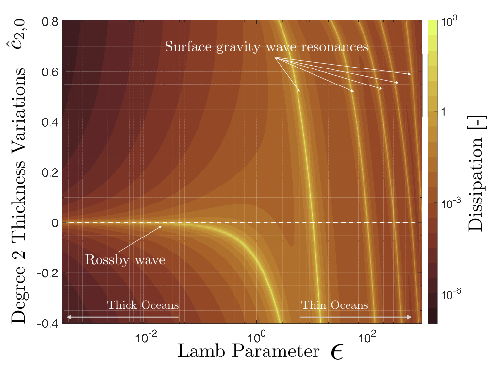
Figure 1: Energy dissipation due to obliquity tides in a surface unstratified ocean with degree two ocean thickness variations.
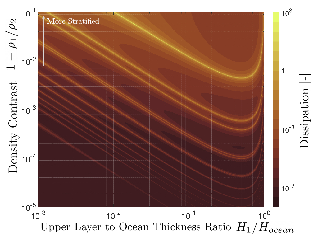
Figure 2: Energy dissipation due to internal waves excited by the eccentricity tide in a stratified subsurface ocean with Lamb parameter 5·10-3 and effective rigidity 10 (similar to Enceladus).
References
Beuthe, M. 2016, Icarus, 280, 278 , doi: 10.1016/j.icarus.2016.08.009
—. 2018, Icarus, 302, 145, doi: 10.1016/j.icarus.2017.11.009
Beuthe, M., Rivoldini, A., & Trinh, A. 2016, Geophys. Res. Lett., 43,10,088, doi: 10.1002/2016GL070650
Câdek, O., Tobie, G., Van Hoolst, T., et al. 2016, Geophys. Res. Lett., 43, 5653, doi: 10.1002/2016GL068634
Hemingway, D. J., & Mittal, T. 2019, Icarus, 332, 111 , doi: 10.1016/j.icarus.2019.03.011
Laplace, P.-S. 1798, Traité de mécanique céleste, Tome II, Livre IV, Des oscillations de la mer et de l’atmosphère
Matsuyama, I., Beuthe, M., Hay, H. C., Nimmo, F., & Kamata, S. 2018, Icarus, 312, 208 , doi: 10.1016/j.icarus.2018.04.013
Ojakangas, G. W., & Stevenson, D. J. 1989, Icarus, 81, 220 , doi: 10.1016/0019-1035(89)90052-3
Tyler, R. H. 2008, Nature, 456, 770, doi: 10.1038/nature07571
How to cite: Rovira-Navarro, M., Matsuyama, I., and Hay, H. C. F. C.: A General Formulation of Thin-Shell Tidal Dynamics, Europlanet Science Congress 2022, Granada, Spain, 18–23 Sep 2022, EPSC2022-24, https://doi.org/10.5194/epsc2022-24, 2022.
1) Introduction
In the context of the Artemis program, the interest of lunar study has been renewed. The Lunar Laser Ranging (LLR) experiment allows since fifty years to determine the Earth-Moon distance at a few centimeters accuracy and the Moon’s librations at a one milliarcsecond accuracy ([4], [3]) Such accuracy allows a refined description of the Moon’s rotation.
The tidal response of the Moon depends on its density and rheology and it affects its rotation. Therefore it provides important information on the lunar internal structure (e.g. [6], [7], [5], [1]). The variation of the harmonic degree 2 gravitational potential due to the tidal response can be quantified by the tidal Love number k2. The latter depends on the forcing frequency, which are mainly exerted by the Earth and the Sun. The dissipation is quantified by the dissipation factor Q which is related to the value of the time delay.
2) Time-delay lunar tides
Furthermore, because of the dissipation due to the viscosity of the lunar interior, the tidal deformation is not instantaneous. The current version of the planetary and lunar ephemeris INPOP only account for unique k2 and time delay [4]. Time delay can be described by a complex Love number k2, which in this case, depends also on the forcing frequency [7]. The dissipation factor Q is related to the imaginary part of the Love number.
Here we explore the introduction of tidal models in numerical ephemerides. We aim to include the k2 and Q frequency dependency in INPOP.
The formulation in Fourier series of the distortion coefficients (also called variation of the Stokes coefficients) by Williams and Boggs (2015) ([7]) allows to describe the tidal gravitational variation in accounting for the frequency dependency of the complex k2. The distortion coefficients vary according to the forcing frequencies formulated as linear combinations of the Delaunay arguments, the latter being described as a polynomial expansion with respect to the time.
3) Representation of the orbit of the Moon
However, the representation in series of the distortion coefficients needs to be consistent with the ephemerides that we use. For that, we can use a semi-analytical representation of the ephemerides.
Numerical ephemerides can described the orbit and the rotation of the Moon with a good accuracy according to the observational error. In complement, the semi-analytical approach is useful to extract information and to disentangle the different physical contributions contains in the numerical approaches. The Éphéméride Lunaire Parisienne (ELP) provides the most accurate semi-analytical model of the orbital motion of the Moon, in the form of Fourier and Poisson series [2].
Figure 1 shows that the difference of the Earth-Moon distance between the solution of INPOP19a and the solution of ELP fitted to INPOP19a reach a maximum value of the order of 4 m. Then, we deduce the amplitude of the distortion coefficients from the fitted semi-analytical representation.

Figure 1. Difference of the Earth-Moon distance between the solution of IN- POP19a and the solution of ELP fitted to INPOP19a. The origin of time is J2000.
References
[1] A. Briaud, A. Fienga, D. Melini, N. Rambaux, A. M ́emin, G. Spada, C. Sal- iby, H. Hussmann, and A. Stark. Constraints on the Moon’s Deep Interior from Tidal Deformation. In LPI Contributions, volume 2678 of LPI Contri- butions, page 1349, March 2022.
[2] J. Chapront and G. Francou. The lunar theory ELP revisited. Introduction of new planetary perturbations. , 404:735–742, June 2003.
[3] Ryan S. Park, William M. Folkner, James G. Williams, and Dale H. Boggs. The JPL Planetary and Lunar Ephemerides DE440 and DE441. , 161(3):105, March 2021.
[4] V. Viswanathan, A. Fienga, O. Minazzoli, L. Bernus, J. Laskar, and M. Gastineau. The new lunar ephemeris INPOP17a and its application to fundamental physics. , 476(2):1877–1888, May 2018.
[5] V. Viswanathan, N. Rambaux, A. Fienga, J. Laskar, and M. Gastineau. Observational Constraint on the Radius and Oblateness of the Lunar Core- Mantle Boundary. , 46(13):7295–7303, July 2019.
[6] James Williams, Dale Boggs, Charles Yoder, James Ratcliff, and J. Dickey. Lunar rotational dissipation in solid body and molten core. Journal of Geo- physical Research, 106:27933–27968, 11 2001.
[7] James G. Williams and Dale. H. Boggs. Tides on the Moon: Theory and determination of dissipation. Journal of Geophysical Research (Planets), 120(4):689–724, April 2015.
How to cite: Baguet, D., Rambaux, N., Fienga, A., Mémin, A., Briaud, A., Hussmann, H., Stark, A., Hu, X., Viswanathan, V., and Gastineau, M.: Introduction of tidal models in lunar ephemerides, Europlanet Science Congress 2022, Granada, Spain, 18–23 Sep 2022, EPSC2022-978, https://doi.org/10.5194/epsc2022-978, 2022.
The ESA/Jaxa mission BepiColombo[1] to Mercury will arrive in orbit in 2025. Onboard is the BepiColombo Laser Altimeter (BELA)[2], which will be used to scan the planetary surface. We plan on using these data to derive the tidal parameter h2[3]. To achieve an accurate result it is necessary to identify and eliminate noise in the laser altimeter records[4]. We present a strategy to find[5], [6] and neutralize the non-Gaussian noise contributions which contribute the most to the uncertainty in the derived Love number.
References
[1] J. Benkhoff et al., ‘BepiColombo—Comprehensive exploration of Mercury: Mission overview and science goals’, Planet. Space Sci., vol. 58, no. 1, pp. 2–20, Jan. 2010, doi: 10.1016/j.pss.2009.09.020.
[2] N. Thomas et al., ‘The BepiColombo Laser Altimeter’, Space Sci. Rev., vol. 217, no. 1, p. 25, Feb. 2021, doi: 10.1007/s11214-021-00794-y.
[3] R. N. Thor et al., ‘Prospects for measuring Mercury’s tidal Love number h2 with the BepiColombo Laser Altimeter’, Astron. Astrophys., vol. 633, p. A85, Jan. 2020, doi: 10.1051/0004-6361/201936517.
[4] O. J. Stenzel, I. Hall, and M. Hilchenbach, ‘Mercury Tide Parameter Estimation from Laser Altimeter Records’, LPI contributions vol. 2678, p. 1990, Mar. 2022.
[5] O. Stenzel and M. Hilchenbach, ‘Towards machine learning assisted error identification in orbital laser altimetry for tides derivation’, pp. EPSC2021-688, Sep. 2021, doi: 10.5194/espc2021-688.
[6] O. Stenzel, R. Thor, and M. Hilchenbach, ‘Error identification in orbital laser altimeter data by machine learning’, pp. EGU21-14749, Apr. 2021, doi: 10.5194/egusphere-egu21-14749.
How to cite: Stenzel, O. and Hilchenbach, M.: Detection and Handling of Noise in Laser Altimetry Data: a Prerequisite for Tides Derivation, Europlanet Science Congress 2022, Granada, Spain, 18–23 Sep 2022, EPSC2022-522, https://doi.org/10.5194/epsc2022-522, 2022.
The classical approach to estimate an asteroid's mass is to analyze its gravitational interactions with another object such as a spacecraft, Mars, a companion asteroid, or a separate asteroid during an asteroid-asteroid close encounter. The latter case leads to gravitational perturbations on a small, generally assumed massless, test asteroid, by the larger perturber asteroid involved in the encounter. By measuring and modeling these perturbations it is possible to estimate the mass of the larger asteroid. This can be described as an inverse problem where the aim is to fit six orbital elements for each asteroid in addition to masses for the perturbing asteroids into astrometric data for each asteroid.
Given that the signals of the perturbations are generally very weak, high precision astrometry and long observational arcs are vital for estimating asteroid masses with acceptable accuracy. It follows that the milliarcsecond-precision astrometry produced by the Gaia spacecraft is a great boon to the field and asteroid mass estimation is considered one of the main applications of Gaia's Solar System Object (SSO) astrometry (Gaia Collaboration et al. 2018a). Indeed, we have recently demonstrated that usage of SSO astrometry from the second Gaia Data Release (DR2) (Gaia Collaboration et al. 2018b) in combination with Earth-based astrometry can reduce the associated uncertainties by up to an order of magnitude in comparison to results computed with Earth-based alone (Siltala & Granvik 2022). In that work, we observed that DR2 does remain limited by the relatively short observational arc of the astrometry as well as the low number (14,099) of asteroids included, which excludes a large number of potentially interesting asteroids.
The third Gaia Data Release (DR3), to be released in June 2022, is expected to remedy these issues to a certain extent. DR3 will include astrometry approximately 11 times more asteroids (158,152) over a much longer timespan. In addition, the SSO data processing has improved and correspondingly we expect further improvements in data quality. Thus, DR3 will enable a large number of asteroid mass estimates beyond what is already possible with DR2 while leading to further improvements to the uncertainties of the masses in cases where DR2 was already usable.
In this presentation, we demonstrate the practical impact of DR3 on asteroid mass estimation. We re-compute asteroid masses from several test cases we previously studied with Gaia DR2 and compare the results to those previously obtained in Siltala & Granvik 2022. Both mass estimation with DR3 alone and in combination with Earth-based astrometry are attempted. Such comparisons will reveal the extent of the improvements to asteroid masses enabled by DR3.
Finally, we briefly discuss future prospects for the application of DR3 to mass estimation, including a comprehensive study of a much larger sample of asteroids,
References
Gaia Collaboration, Spoto, F., Tanga, P., Mignard, F., and 621 co-authors (2018a). Gaia Data Release 2. Observations of solar system objects. A&A, 616:A13.
Gaia Collaboration, Brown, A. G. A., Vallenari, A., Prusti, T., and 621 co-authors (2018b). Gaia Data Release 2. Summary of the contents and survey properties. A&A, 616:A1.
Siltala, L. and Granvik, M. (2022). Masses, bulk densities, and macroporosities of asteroids (15) Eunomia, (29) Amphitrite, (52) Europa, and (445) Edna based on Gaia astrometry. A&A, 658:A65.
How to cite: Siltala, L. and Granvik, M.: Asteroid Mass Estimation with the Third Gaia Data Release, Europlanet Science Congress 2022, Granada, Spain, 18–23 Sep 2022, EPSC2022-1081, https://doi.org/10.5194/epsc2022-1081, 2022.
Introduction
Current and future small body missions, such as the ESA Hera mission [1] or the JAXA MMX mission [2] demand good knowledge of the gravitational field of the targeted celestial bodies. This is not only motivated to ensure the precise spacecraft operations around the body, but likewise important for landing manoeuvres, surface (rover) operations, and science, including surface gravimetry [3]. To model the gravitation of irregularly-shaped, non-spherical bodies, different methods exist. Previous work performed a comparison between three different methods [4], considering a homogeneous density distribution inside the body. In this work, the comparison is continued, by introducing a first inhomogeneity inside the body. For this, the same three methods, being the polyhedral method [5] and two different mascon methods [6][7] are compared. We will describe the methods and our test cases in the next Section.
Methodology
The polyhedral method (PM) provides an analytical solution to the gravitational potential field of any polyhedral body [5]. Intrinsically, the method demands a homogeneous density throughout the body, making it not directly applicable to account for inhomogeneities. Therefore, in this work, we perform a superposition of the gravitational fields of the main body and the inhomogeneities, considering the differential density, which can also be negative.
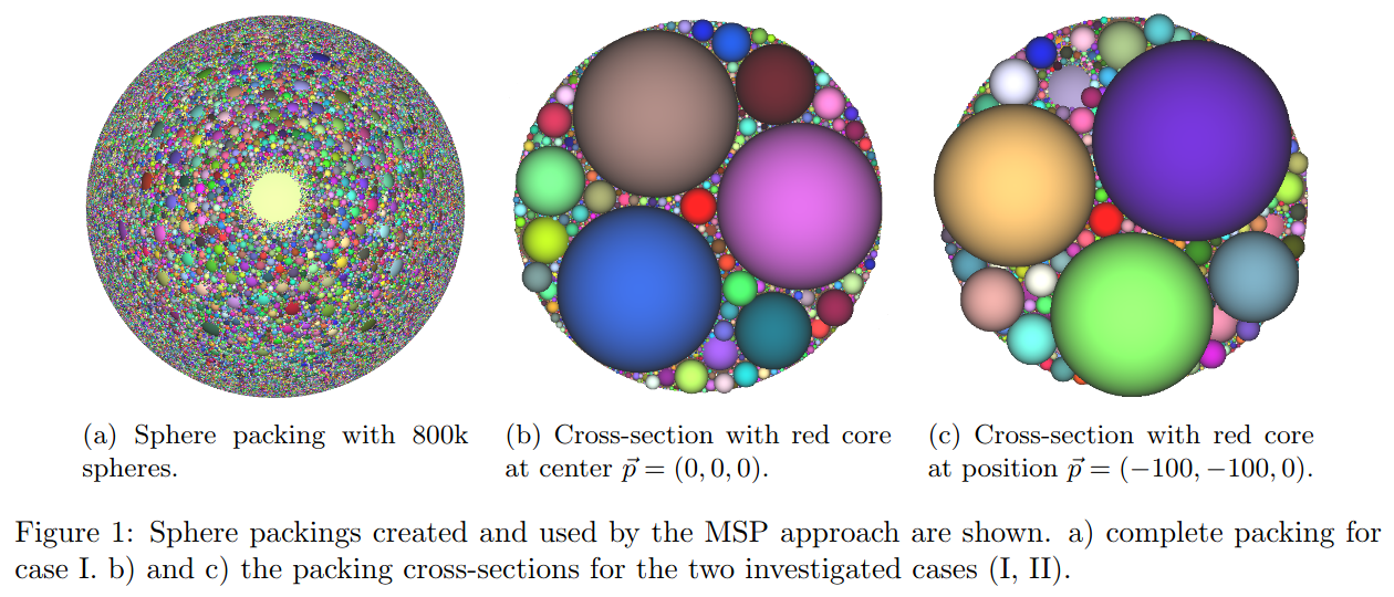
The other two methods are based on mascons, namely MSP (Mascons: Sphere Packing) and MASC (Mascons: Spherical Coordinates). These mascon methods subdivide a body into smaller parts. The mass is then concentrated in the centre of these parts and the gravitational field is the sum of the individual accelerations. MSP uses a sphere packing with non-uniform-sized spheres that do not overlap (see Fig.1). Since the sphere packing does not cover the complete volume, we use additionally a heuristic that tends to assign smaller spheres more mass. To model inhomogeneity, we compute separate sphere packings with different densities assumed. With MASC, the internal mass distribution is modelled by dividing the body in longitude, latitude, and radius, and by assigning individual densities to the resulting set of tesseroids.
Test Cases
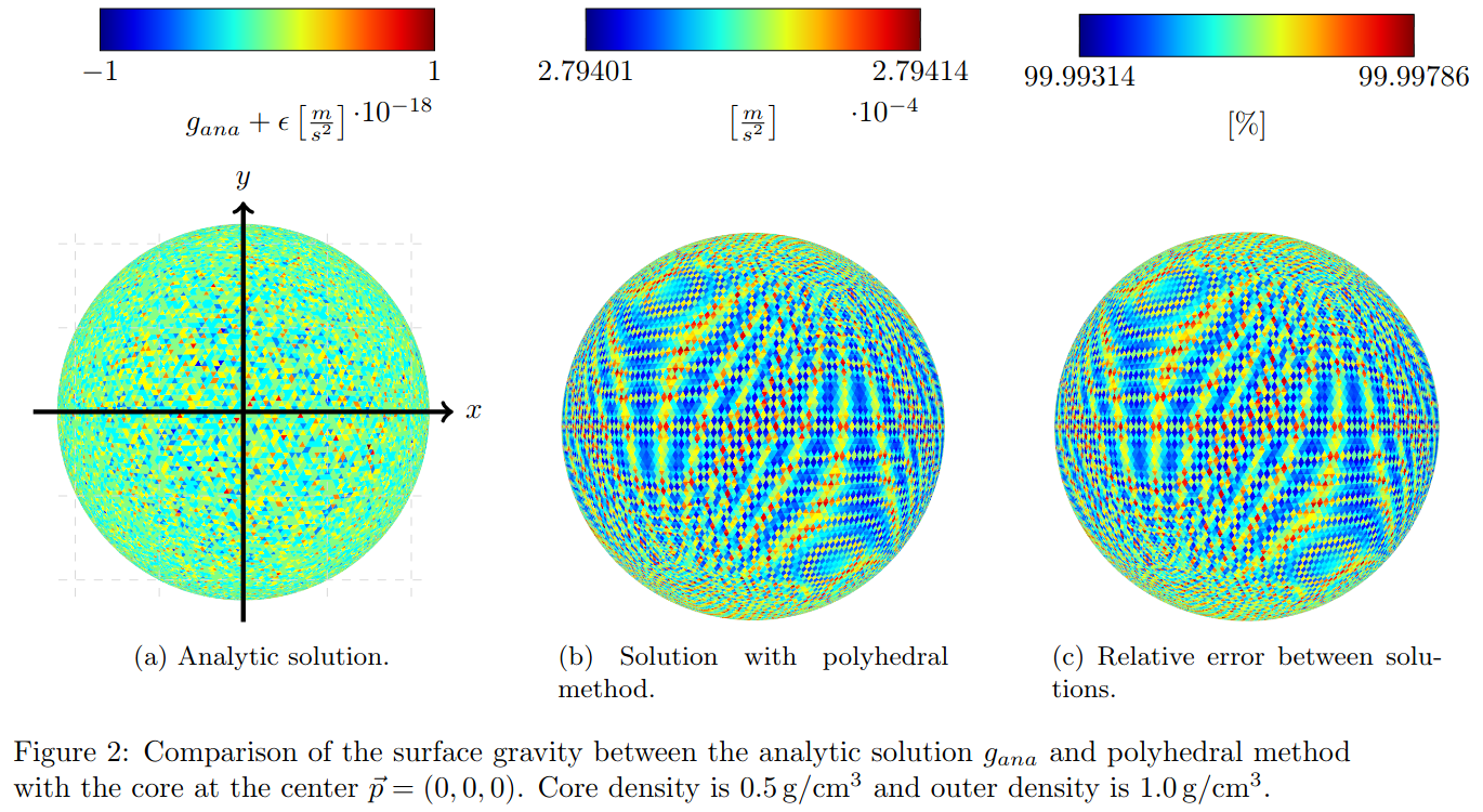
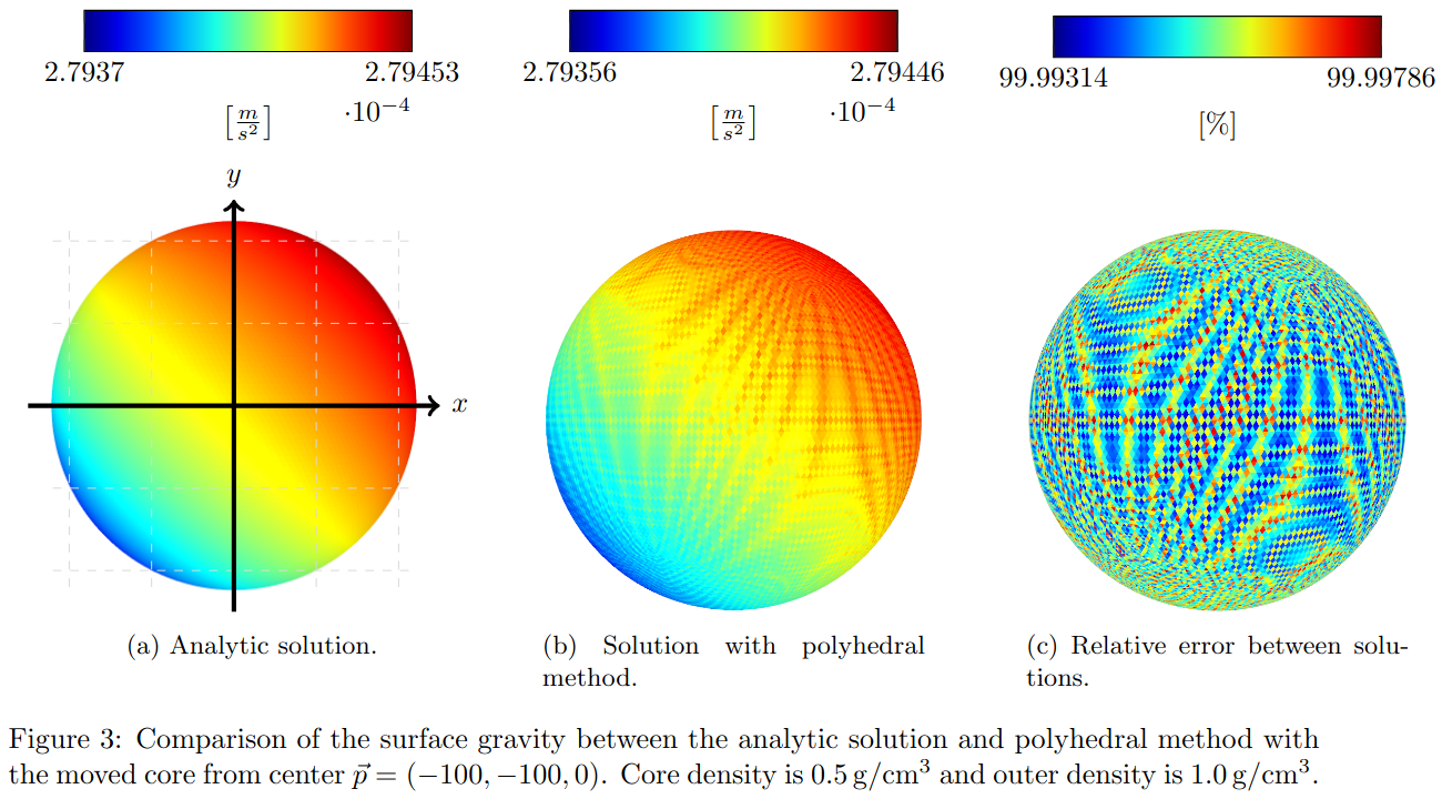
Our two test cases consider two nested ideal spheres that are approximated through a UV-Sphere with 328,328 facets [4]. The outer sphere has a radius r=1,000 m and a density of 1.0g/cm³, and the inner sphere has a radius r=100 m and a density of 0.5g/cm³. In Case I, the inner sphere is placed concentric to the outer sphere, whereas in Case II the sphere’s centre is translated to X=−100 m and Y=−100 m. We compute the gravitational acceleration for points on the ideal sphere and compare it to the analytical solution through a relative error. Clearly, the ratio of computed and analytical solution τ =gcom /gana should always be <100% as the UV-sphere is only an approximation of the perfect sphere, values >100% represent an overshoot. This agreement ratio is presented in the next Section.
First Results
The overall results and range of τ on the surface of the sphere are summarized in Table 1:
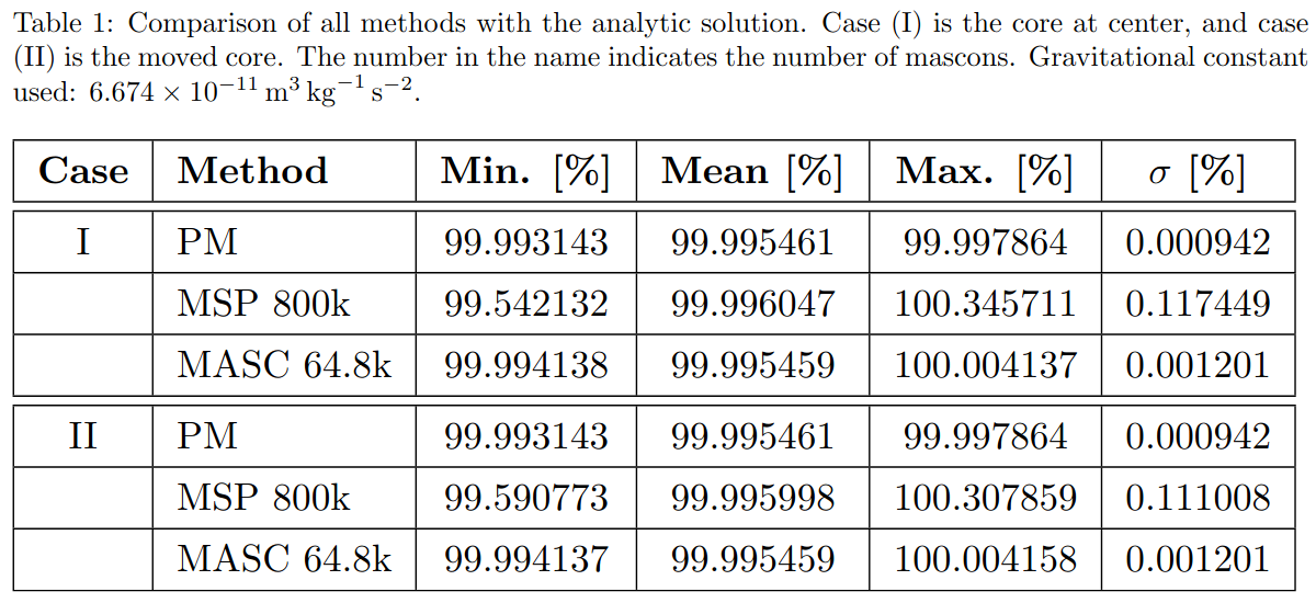
For both of our cases, PM delivers the most accurate results (Table 1). The error results from the shape approximation. It is visualized in Figures 1 and 2. We can see the expected shift from an almost equal to an unequal surface gravity. In Figure 1 we can also see that the shape approximation error is larger than the floating-point precision limitation (noisy pattern, Figure 1a).
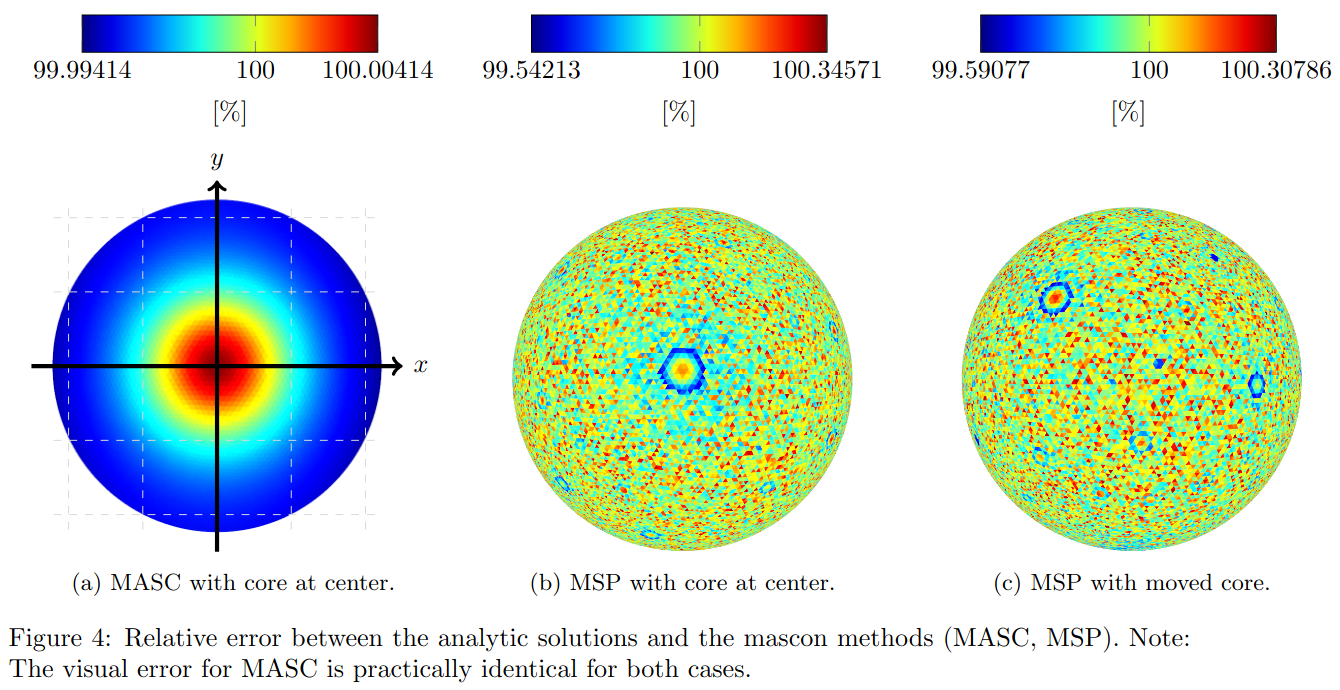
The MSP method creates a noisy overshooting pattern (see Figures 4b and 4c), which results from the spheres near the surface and the heuristic. Large spheres lead to a circular artifact at the surface. Observable at the center of Figures 4b and 1a. It is a similar pattern for Case II. The MASC error results from the subdivision in spherical coordinates. At the poles the number of tesseroids increases, which leads to a circular overshoot at two sides. It is also true for the shifted core (see Figure 4a). The computation time for MSP remained the same as for the homogeneous case [4] while it has doubled for PM and MASC.
The three methods presented above for the computation of the gravitational acceleration will be applied to more complex shapes for irregularly shaped bodies. In addition, different inhomogeneous density distributions representing the interior will be studied and the according results presented.
Acknowledgements
M.N. acknowledges funding from the Foundation of German Business (sdw) and the Royal Observatory of Belgium (ROB) PhD grants. The work by Bundeswehr University was carried out in the frame of project KaNaRiA-NaKoRa which is funded by DLR under grant FKZ50NA1915. The work on the part of University of Bremen presented in this paper was partially funded by DLR under grant 50NA1916.
References
[1] Michel, Patrick, et al. "The Hera mission: European component of the ESA-NASA AIDA mission to a binary asteroid." 42nd COSPAR Scientific Assembly 42 (2018):B1-1.
[2] Campagnola, Stefano, et al. "Mission analysis for the Martian Moons Explorer (MMX) mission." Acta Astronautica 146 (2018):409-417.
[3] Noeker, Matthias, et al. "The GRASS Gravimeter Rotation Mechanism for ESA Hera Mission On-Board Juventas Deep Space CubeSat." Proceedings of the 46th Aerospace Mechanisms Symposium, Virtual, May 11-13, (2022):159-172.
[4] Meißenhelter, Hermann, et al. "Efficient and Accurate Methods for Computing the Gravitational Field of Irregular-Shaped Bodies." 2022 IEEE Aerospace Conference. IEEE, 2022.
[5] Werner and Scheeres. "Exterior gravitation of a polyhedron derived and compared with harmonic and mascon gravitation representations of asteroid 4769 Castalia." Celestial Mechanics and Dynamical Astronomy 65.3 (1996):313-344.
[6] A. Srinivas, et. al. “Fast and accurate simulation of gravitational field of irregular-shaped bodies using polydisperse sphere packings.” in ICAT-EGVE, 2017, pp.213–220.
[7] M. Pätzold, et. al. “Phobos mass determination from the very close flyby of Mars Express in 2010,” Icarus, vol. 229, pp. 92–98, Feb.2014.
How to cite: Noeker, M., Meißenhelter, H., Andert, T., Weller, R., Karatekin, Ö., and Haser, B.: Comparing Methods for Gravitational Computation: Studying the Effect of Inhomogeneities, Europlanet Science Congress 2022, Granada, Spain, 18–23 Sep 2022, EPSC2022-562, https://doi.org/10.5194/epsc2022-562, 2022.
1. Introduction
With the increasing interest in the Solar System's smaller bodies, quite a few missions have been sent to comets and asteroids, and more will be send in the near future. Due to the large distances involved, communication to command mission parameters takes a long time, which has a negative impact on operational safety. Autonomous navigation would be one of the key technologies that can make asteroid missions more robust, safe, and cost effective. This is especially true if one considers the unknown flight environment when the spacecraft is first encountering the body. Most asteroids and comets have a very irregular shape and unknown mass distribution. Therefore, knowledge about its irregular gravity field will be directly beneficial as input to orbital corrections and manoeuvre planning.
2. Methodology
Based on a detailed ``real-world'' simulator, orbits around a small body, here the asteroid Eros-433, can be simulated that are perturbed by non-linear gravity effects, as well as solar-radiation pressure and third-body perturbations. Measuring land marks on the small-body's surface, processed (in a preliminary mission phase with Earth in the loop) to a detailed land-mark database, can be subsequently used to determine the (relative) position and velocity of the spacecraft with respect to the body. A next step would be to use measurements of orbital perturbations to estimate as many components of the body's gravity field as possible. Detailed knowledge about the gravity field can then be used for planning science and mission operations, such as orbital corrections. An in-house code is used to determine the spherical-harmonics coefficients Cnm and Snm, assuming an average asteroid density of 2.6212 g/cm3.
Part of the navigation system are simplified sensors, which provide noisy position and/or velocity measurements. Interfacing with more realistic sensors is possible, but left as future work. The core of the navigation system is an augmented state estimator, based on the unscented Kalman filter for its applicability to highly non-linear systems.
3. Results
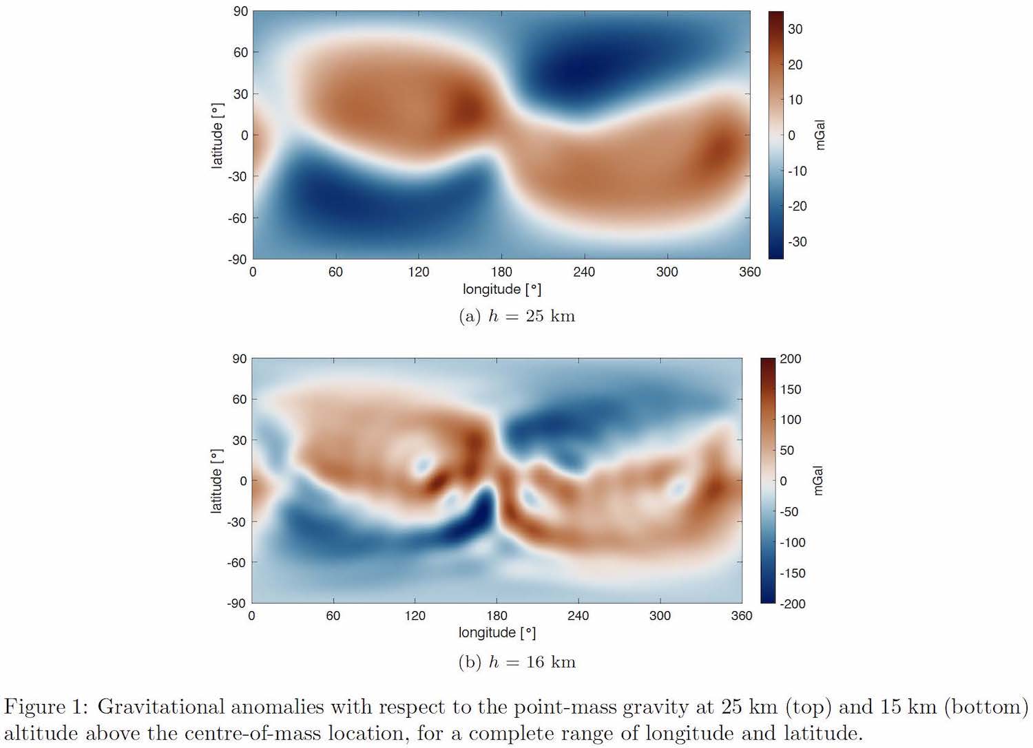
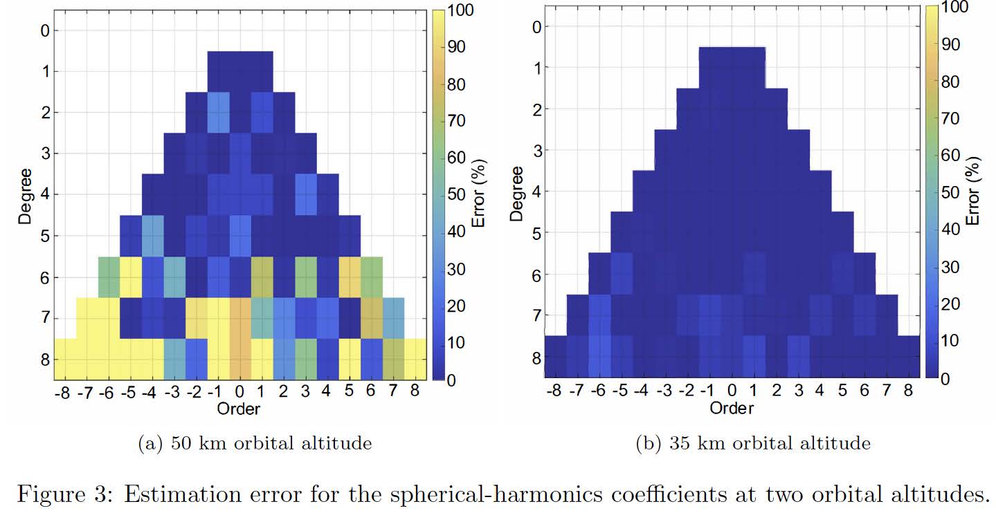
Eros-433 is an elongated body, roughly resembling an ellipsoid, with dimensions of 33 by 13 by 13 km, and rotates with an approximate constant rate in 5.27 hours. For the ``real-world'' asteroid model, a gravity field up to order and degree 16 has been determined, see Figure 1. The results shown are the deviations from the point-mass model and thus highlighting the irregularities of Eros' gravity field. With increasing altitude these irregularities are much more ``smeared out'' and will thus be harder to estimate.
The first simulations that were done aimed at estimating the central-field parameter, μ, and the first zonal harmonic, J2 = C2,0. To do so, several orbital altitudes ranging from 1500 down to 150 km were chosen. In terms of measurements data, it was assumed that only noisy position and velocity data were available at a frequency of 1 Hz. Figure 2 shows the estimates of μ. The remaining error is well below 0.1% for the different altitudes. With the estimated value of μ substituted in the filter, the estimate of J2 is seen to converge best at an altitude of 45 km: at higher altitudes the J2 effect starts to decrease and becomes less noticeable, whereas at lower altitudes the effect of the higher-order terms start dominating. The remaining error is about 6%.

The last part of the research focusses on the estimation of higher-order coefficients. Idealised noisy position (noise level 10 m, which would be possible with current sensor technology) and velocity measurements are used, supported by ideal range measurements at 2 Hz. Figure 3a displays the errors of the full 8 degree and order coefficients for the estimation at an orbital height of 50 km. The coefficients of degree 6 and higher have significant errors, but the coefficients up to degree and order 5 can be estimated within errors of less than 30%. However, once μ and J2 have been estimated and subsequently put to constant values in the estimator, the estimation accuracy significantly improves, but only when the orbit is lowered to 35 km and the measurement time is extended to 10 days (Figure 3b). The average error is about 10%, with a few outliers. These errors are quite small, because of the relatively ideal measurements. Follow-on research should therefore focus on realistic sensor modelling and including instrument errors to the augmented state.
How to cite: Mooij, E., Root, B., and Bourgeaux, A.: Asteroid Gravity-Field Estimation, Europlanet Science Congress 2022, Granada, Spain, 18–23 Sep 2022, EPSC2022-511, https://doi.org/10.5194/epsc2022-511, 2022.
The ideal conditions for RS measurements require an optimization of the communications and tracking systems, the spacecraft trajectories and mission operations for RS investigation. However, these ideal conditions are rarely achieved because of the several trades off that should be made with many other mission and science requirements. This is particularly true for missions in the Neptune system where the identified scientific goals are broad and varied.
The exploration of Triton has been always identified as a key science goal for such a mission. In fact, Neptune’s largest moon Triton is presumably one of the ocean worlds in the outer solar system. With its own atmosphere, active geology, plumes of nitrogen gas and dust entrained deposited up to 150 km downwind, Triton intrigues planetary scientists, who proclaimed it as key ‘ocean world’ for future exploration [1]. According to space agencies’ long term plans (e.g. the US decadal surveys in planetary science, the ESA Cosmic Vision 2 and Voyage 2050 programs), Triton will certainly be visited by the end of the 21st century as also recommended by the radio-science (RS) community which declared Triton’s liquid layer investigation a “key RS goal” [2]. As a result of the general enthusiasm for Triton and similar icy moons of the outer solar system, several mission concepts have recently been proposed, all within the 2029–2035 time frame (e.g. [3-8]).
According to the mission designs proposed in literature, most of the time Neptune is identified as the main target, but fly-bys of Triton will provide in-situ measurements whether there will be just one as Voyager 2 did and the TRIDENT team proposed [9], or multiple fly-bys by leveraging particular Neptune centric orbit (periodic and quasi-synchronous orbits) as Cassini did in the Saturn system or the as the “Triton tour” proposed by the Neptune Odyssey mission concept [10].
We focus on gravity science, i.e. the study of gravitational field with the purpose of inferring planetary properties such as bulk mass, mass/density distribution, internal density gradients, and interior structures and composition. In fact, radio tracking observations of changes in the velocity vectors of a spacecraft as it flies near Triton can be used to define the gravitational field.
We perform a sensitivity study in order to asses the expected precision of the gravity recovery of a combination of different onboard instrumentation, trajectory geometries and radio science experiment configurations. In particular, we perform a covariance analysis in order to determine how the precision in the estimated parameter depend upon the various characteristics of an RS campaign, including:
- Orbit geometry
- Measurement accuracy/data quality (Doppler noise)
- Nongravitational forces
- Arc length
- Mission duration
As an example of the proposed discussion, in Fig.1 we investigated the impact of different orbit geometries: we perform a covariance analysis on several fly-by geometries (see Fig.2), simulating Doppler tracking data performed with an onboard coherent X-band transponder and an High Gain Antenna (accuracy of 0.1mm/s at 60s integration time) over an 8h long arc. We modeled the gravity field the as a spherical harmonic expansion characterized by the Cl,m, Sl,m coefficients [11]. Since the spherical harmonics of Triton have never been measured, we used the Kaula power law in order to have an estimation of the power spectrum of the gravity field. Given the Doppler geometry configuration and relative position between Triton and the Earth in January 2030, we see that the C2,1 and S2,1 will be better determined if the spacecraft has an highly inclined orbit, whereas the estimation of C2,2 and S2,2 has a low uncertainty with slightly inclined orbits.
Similar sensitivity analyses will be discussed over a wide range of mission scenarios, that is with different values for the aforementioned RS settings. The end goal of this study is to provide not only the optimal combination of these settings, but a complete parametric study that will help the design of a future mission to Triton.


Acknowledgments
This work was financially supported by the French Community of Belgium within the framework of the financing of a FRIA grant.
References
[1] Hendrix, A.R. et al., jan 2019. doi:10.1089/ast.2018.1955.
[2] Asmar, S. et al., mar 2021. doi:10.3847/25c2cfeb.9d29ef85.
[3] Arridge, C. et al. ,104:122–140, dec 2014. doi:10.1016/j.pss.2014.08.009.
[4] Hofstadter, M. et al., Planetary and Space Science, 177:104680, nov 2019. doi:10.1016/j.pss.2019.06.004.
[5] Masters, A. et al., Planetary and Space Science, 104:108–121, dec 2014. doi:10.1016/j.pss.2014.05.008.
[6] Simon, A.A., Stern, S.A. and Hofstadter, July 2018.
[7] Simon, A.A. et al., feb 2020. doi:10.1007/s11214-020-0639-1.
[8] Turrini, D. et al., Planetary and Space Science, 104:93–107, dec 2014. doi:10.1016/j.pss.2014.09.005.
[9] Prockter, L.M. et al., In Lunar and Planetary Science Conference, Lunar and Planetary Science Conference, page 3188, Mar. 2019.
[10] Rymer, A.M. et al., sep 2021. doi:10.3847/psj/abf654.
[11] Kaula, W.M. Theory of satellite geodesy. Applications of satellites to geodesy. 1966.
How to cite: Filice, V., Le Maistre, S., and Goosse, H.: Sensitivity of Triton gravity field of different radio science experiment configurations, Europlanet Science Congress 2022, Granada, Spain, 18–23 Sep 2022, EPSC2022-1162, https://doi.org/10.5194/epsc2022-1162, 2022.
Introduction
Rovers, both crewed and robotic have a long tradition in Solar System exploration. Most notably, Lunar and Martian exploration made use of vehicles to explore the surface, including three lunar roving vehicles carrying Apollo astronauts and equipment [1]. More recently, small body (SB) exploration missions started to have landers with mobility included in their mission architectures. The MINERVA-II rovers were part of the Hayabusa2 mission [2] and the two successful rovers became the first rovers on an asteroid, followed by the MASCOT rover [3]. All these probes are referred to as “rovers” as they moved around the surface, irrespective of the movement being realized by hopping, rather than driving. Regarding the latter, the Martian Moon eXplorer (MMX) mission will include a rover with “classical” wheeled locomotion to explore the Phobian surface [4]. Such missions demand careful surface traverse planning, and detailed gravity simulations, taking into account the local topography, being beneficial for both rover operations and the mission’s science return. A prime example for a science application is the use of a surface gravimeter, such as the Apollo 17 TGE [5], or the GRASS gravimeter under development for the ESA Hera mission [6, 7]. This work presents a traverse simulator for local locomotion, accounting for local topography when computing the resulting surface gravity.
Methodology
The Traverse And Gravity Simulator (TAGS) is built upon the Wedge-Pentahedra Method (WPM) [8]. This method allows precise, high-resolution surface representation, and the assessment of the local terrain’s influence on the (surface) gravitation (topographic correction). In continuation of previous work [8], the evaluation location in the TAGS is varied to represent a surface (rover) traverse. The 3D-orientation of the gravitation vector is computed, and hence the variation of the vector orientation with respect to the initial reference gravitation along the traverse is plotted in the simulator. Likewise, the resulting gravity gres and the “vertical” component gz along the rover traverse is plotted, illustrating the variations over the non-spherical body’s surface, and due to the local (artificial) topography. Variation of the terrain scale factor ST further allows to compare the influences of terrain with variable amplification, where larger scale factors are representative of larger terrain amplitudes, e.g. higher hillocks and deeper craters. While the WPM is only concerned with gravitation, the TAGS is purposely referring to gravity, as the simulator will allow to include additional (dynamical) effects to the resulting gravity, such as the contributions form rotation, libration and tides.
Applications
To show the TAGS working and illustrate the local surface gravity variations, a rover traverse on the Martian moon Phobos has been simulated. Starting in the centre of the terrain, the traverse step between the individual evaluation points are +50 m in +X-direction, and −50 m in –Y-direction for both routes. TAGS simulation results for a total of twelve gravity evaluation stations is plotted in Figures 1 and 2 for which two different terrain scale factors (amplification of local topography) ST = 100 and ST = 500 are used.
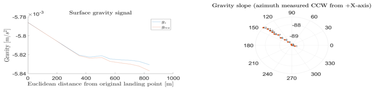
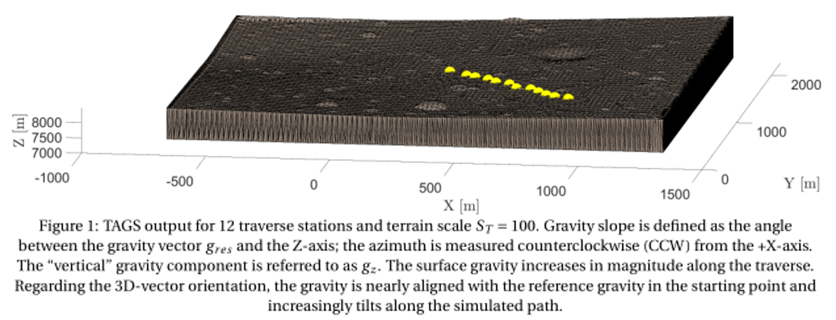
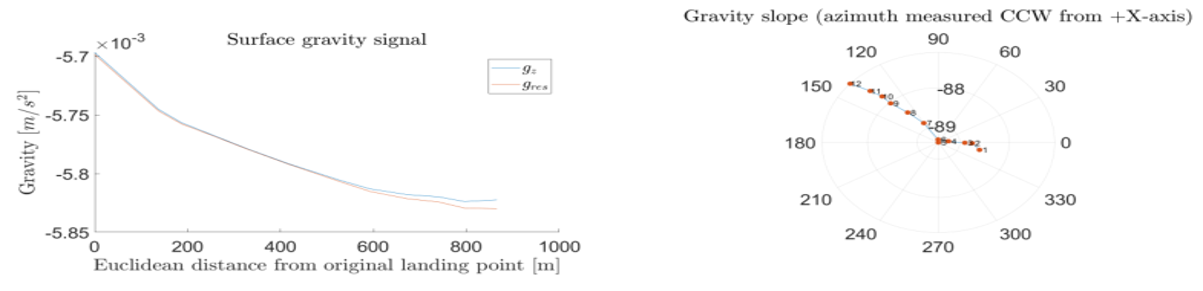
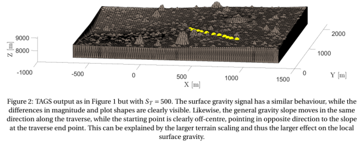
Regarding the surface gravity signal in the two compared rover traverses, the overall gravity signal is similar in both magnitude and increasing trend along the traverse. However, the TAGS simulation likewise clearly illustrates the gravity differences experienced in both traverses, due to the local topographical differences. For ST = 100, the resulting gravity gres ranges from (5.786 – 5.837) ×10-3 m/s², whereas for ST = 500, gres is ranging from (5.698 – 5.830) ×10-3 m/s². The larger terrain scaling (ST = 500) results in a gravity 1.521 % and 0.120 % smaller compared to the “flatter” terrain (ST = 100), for the lower and upper limit, respectively. In addition, it can be well observed that the “vertical” Z-component of the gravity gz diverges from gres, caused by increasing gravity vector inclinations with respect to the reference gref, likewise well observable in the TAGS polar plots (2.7° for ST = 100; 2.9° for ST=500).
Outlook
We will quantify the local terrain’s influence on the surface gravity along the traverse, which has implications both on surface sciences (e.g. gravimetry) and landing/surface operations. This is specifically important, as the WPM considers high-resolution digital elevation models on a local scale with a ground resolution much better than the global shape file resolution of the target (small) body. The here presented Traverse And Gravity Simulator (TAGS) allows for detailed traverse planning of exploratory rovers on extraterrestrial surfaces, both using artificial and newly obtained (real) local terrain data. TAGS can be extended in its applications, e.g. by integrating dynamical contributions to gravity, simulating illumination conditions, or for public outreach and education.
Acknowledgements
M.N. acknowledges funding from the Foundation of German Business (sdw) and the Royal Observatory of Belgium (ROB) PhD grants. The authors acknowledge funding from BELSPO via the PRODEX Programme of ESA and from the European Union’s Horizon 2020 research and innovation program under grant agreement No. 870377 NEO-MAPP.
References
[1] Asnani, Vivake, et al. “The development of wheels for the Lunar Roving Vehicle.” Journal of Terramechanics 46.3 (2009): 89-103.
[2] Van Wal, Stefaan, et al. “Prearrival deployment analysis of rovers on Hayabusa2 asteroid explorer.” Journal of Spacecraft and Rockets 55.4 (2018): 797-817.
[3] Ulamec, Stephan, et al. “Landing on small bodies: From the Rosetta Lander to MASCOT and beyond.” Acta Astronautica 93 (2014): 460-466.
[4] Michel, Patrick/Ulamec, Stephan, et al. “The MMX rover: performing in situ surface investigations on Phobos.” Earth, Planets and Space 74.1 (2022): 1-14.
[5] Talwani, M., et al. “13. Traverse Gravimeter Experiment” Apollo 17: Preliminary Science Report (1973): 13-1 – 13-13.
[6] Karatekin, Özgür, et al. “Surface gravimetry on Dimorphos.” EGU General Assembly Conference Abstracts. 2021.
[7] Noeker, Matthias, et al. “The GRASS Gravimeter Rotation Mechanism for ESA Hera Mission On-Board Juventas Deep Space CubeSat.” Proceedings of the 46th Aerospace Mechanisms Symposium, Virtual, May 11-13, (2022): 159-172.
[8] Noeker, Matthias, et al. “Artificial terrain on Phobos: Assessing the influence on local gravity using the Wedge-Pentahedra Method” No. EPSC2021-370. Copernicus Meetings, 2021.
How to cite: Noeker, M. and Karatekin, Ö.: Gravity Traverse Simulations for Small Bodies and Moons of the Solar System using the Wedge-Pentahedra Method, Europlanet Science Congress 2022, Granada, Spain, 18–23 Sep 2022, EPSC2022-361, https://doi.org/10.5194/epsc2022-361, 2022.
Ejection of solid bodies from comets and its dynamical significance for velocity and rotation of comet
Introduction
Observations of comets 9P/Tempe 1 and 67P/Churyumov – Gerasimenko revealed existence of several ejections of significant masses [1, 2, 3].
In the present paper we investigate dynamic effects for the comet of similar ejections. Contrary to research presented in [6], we consider here ejections with higher velocity, i.e., 0.71 m s-1 or higher from different places mainly on the surface of the comet 67P/Churyumov – Gerasimenko and some our model body.
Gravitational field and mechanism of ejection
The gravitational field of considered comet is complicated [1, 4]. There are several regions of different slopes of the comet's surface in respect to the local gravity. Note also non-spherical shape of cometary surface of constant potential [6].
In [6] there are considered slow ejecta (i.e. ejecta with velocity below escape velocity). Here we consider the ejecta with the velocity 0.71 m s-1 or higher. Often, the initial velocity is higher than the escape velocity. Note, however, that the for comets of irregular shape, the escape velocity depends strongly on the site of ejection.
A following model of processes leading to the ejection is assumed. It is based on [3, 4]. The phase changes supply the heat to a certain underground volume. If the pressure exceeds some critical value then some fragments will be ejected into space. Many places in the comet could be a result of such processes [3]. Note that the initial velocity of ejecta are assumed to be perpendicular to the physical surface. This assumption is used successfully in [4].
Calculations
We consider ejecta from different places on comet 67P/G-C. For the comet dynamical effects of slow ejecta is more limited but also more complicated because the comet obtained back some momentum and spin from the landing ejecta.
We performed calculations for 530 ejected particles from different places in the comet 67P/C-G and some for our model body. Total mass of ejecta for the comet 67P is chosen to be: 10-6 or 10-5 of the mass of the whole comet. These values correspond to ~105 kg and ~106 kg for each ejected particles (it depends on the number of particles used for given calculation). The following velocities of ejecta are used: 0.7, 1.0, 10 m s-1. Other values are used for the model body. For calculations the program developed by L. Czechowski was used.
Preliminary results and conclusions
In general, the effect of ejecta on comet's motion is primarily determined by the total momentum and angular momentum of the ejected particles. However, unlike the gases ejected by comet jets, the movement of solid particles depends heavily on the comet's gravitational field. The solid particles can return to the comet, giving up some of their momentum. Therefore, they have a different effect on comet motion and should be taken into account in more accurate calculations of comet's motion.
Acknowledgements
The research is partly supported by Polish National Science Centre (decision 2018/31/B/ST10/00169)
References
[1] Czechowski L., (2017) Dynamics of landslides on comets of irregular shape. Geophysical Research Abstract. EGU 2017 April, 26, 2017
[2] Jorda, L., R. et al. (2016) The global shape, density and rotation of Comet 67P/Churyumov-Gerasimenko from preperihelion Rosetta/OSIRIS observations, Icarus, 277, 257-278, ISSN 0019-1035, https://doi.org/10.1016/ j.icarus.2016.05. 002.
[3] Kossacki K., Czechowski L., 2018. Comet 67p/Churyumov–Gerasimenko, possible origin of the depression Hatmehit. Icarus vol. 305, pp. 1-14, doi: 10.1016/j.icarus.2017.12.027
[4] Czechowski L. and Kossacki K. J. 2021. Dynamics of material ejected from depression Hatmehit and landslides on comet 67P/Churyumov–Gerasimenko. Planetary and Space Science 209, 105358, https://doi.org/10.1016/j.pss.2021. 105358
How to cite: Czechowski, L.: Ejection of solid bodies from comets and its dynamical significance for velocity and rotation of comet, Europlanet Science Congress 2022, Granada, Spain, 18–23 Sep 2022, EPSC2022-1029, https://doi.org/10.5194/epsc2022-1029, 2022.
Please decide on your access
Please use the buttons below to download the presentation materials or to visit the external website where the presentation is linked. Regarding the external link, please note that Copernicus Meetings cannot accept any liability for the content and the website you will visit.
Forward to presentation link
You are going to open an external link to the presentation as indicated by the authors. Copernicus Meetings cannot accept any liability for the content and the website you will visit.
We are sorry, but presentations are only available for users who registered for the conference. Thank you.
Posters: Mon, 19 Sep, 18:45–20:15 | Poster area Level 1
The Mars Global Surveyor (MGS), Mars Odyssey (MO), and Mars reconnaissance Orbiter (MRO) Doppler tracking data from 1999 to end of 2021 have been reprocessed, offering the longest time series ever obtained for the gravity field of a planet.
The process, called Precise Orbit Determination (POD), uses the Doppler radio-tracking data acquired at the Deep Space Network (DSN) ground stations, and an accurate dynamical model for each spacecraft. This model employs identical up-to-date standards and state-of-the-art of the force models, both surface forces and gravitational forces. A macromodel of each spacecraft (surface area and optical properties of the faces of the probe) is taken into account. It is oriented in space at any time given telemered quaternions. This attitude information of the bus of the spacecraft is completed by the attitude of the articulated solar array and of the steerable high gain antenna with respect to the spacecraft body. In addition, the self-shadowing effect is introduced for each surface force, atmospheric drag and radiation pressure form the Sun and the planet (albedo and infra-red emission). The angular momentum desaturation maneuvers are taken into account by solving for empirical accelerations at the epoch of each maneuver.
This force model allows to compute theoretical Doppler tracking data, then the difference of these predicted data with the tracking data collected at ground stations is computed. Least square fit of this difference is processed over successive data-arcs with a duration of 4 days for each spacecraft. This least squares filter allows to adjust a scale factor of the drag and solar pressure force for each data-arc as well as residual accelerations at each angular momentum desaturation event. The least squares fit results in normal matrices for each data-arc and for each spacecraft. It contains partial derivatives for each coefficient of the force model (scale factors, residual accelerations) as well as for the time series the first zonal gravity field coefficients and for the degree 2 tidal Love number, k2. All the normal matrices are stacked together in order to retrieve a time series of the gravity field from 1999 to 2021 (about 10 Martian year), which has never been obtained before. The k2 Love number solution is also re-estimated. We analyze the error on the obtained solution depending on the number of satellite we used (1 to 3) and the data timespan used.
The retrieved time-varying gravity coefficients and the Love number k2 are then use to tightly constrain the seasonal variations in the mass of the polar caps and the solid tides of Mars, respectively
How to cite: levesque, M., rosenblatt, P., marty, J., and dumoulin, C.: Update of seasonal gravity field and k2 love number of Mars from MGS, Mars Odyssey and MRO radio science, Europlanet Science Congress 2022, Granada, Spain, 18–23 Sep 2022, EPSC2022-392, https://doi.org/10.5194/epsc2022-392, 2022.
Introduction
The orientation of Mars with respect to its orbit can be described with a set of Euler angles (longitude ψ, obliquity ε, and rotation φ). The rotation model for Mars, as described in the Barycentric Celestial Reference System (BCRS), includes two relativistic contributions: (1) a contribution to the precession and nutations in longitude which mainly comes from the Geodetic effect, (2) a contribution to the variations in rotation angle which mainly comes from the reference frame transformation between the local Martian frame and the BCRS frame and their respective time. We present a new estimation of the two relativistic contributions to Mars orientation.
Results
We compute the geodetic and Lense-Thirring effects. The geodetic effect (e.g. Fukushima, 1991, Baland et al. 2020) is due to Mars motion along its orbit and only affects the longitude angle with precession and nutations terms:
ψgeodetic(t) = 6.754 mas/yr t + 0.565 mas sin l + 0.039 mas sin 2l + 0.004 mas sin 3l,
l being the mean anomaly of Mars. The Lense-Thirring effect is due to the rotation of the Sun, and affects the three orientation angles (e.g. Barker and O’Connell, 1970, or Poisson and Will, 2014). We find that the Lense-Thirring effect is 4 to 5 orders of magnitude smaller than the geodetic effect.
Another relativistic correction [φ]GR(t) must be included in the model for the rotation angle (e.g. Eq. (18) of Konopliv et al. (2006), after Yoder and Standish 1997, with annual, semi-annual, and ter-annual terms, and amplitudes in mas) :
[φ]GR(t) = - 175.80 sin l - 8.20 sin 2l - 0.60 sin 3l.
This correction is obtained as the product of the mean rotation rate and of the difference between the local Martian time and the Barycenteric Dynamical Time. This time difference is related to relativistic time transformation between reference frames and is impacted by the velocity of Mars with respect to the solar system barycenter and by the gravitational potential experienced by Mars in its motion. We update the estimation of Yoder and Standish (1997), using three independent approaches: (1) a toy model where the planets evolve on Keplerian orbit, (2) a fit to a numerical integration using the DE440 planetary ephemerides (Park et al. 2021), (3) a computation using the analytical planetary theory VSOP87 (Bretagnon & Francou 1988). We obtain a solution of the form:
[φ]GR(t) = φ'GR t + Σj φj sin (fj t + ξj),
with φj the amplitudes, fj the angular frequencies, and ξj the phases at t=0 of a periodic series. This solution includes seasonal terms with amplitudes which differ from those of Yoder and Standish, (1997), e.g. by about 10 mas for the annual term, which is 10 times larger than the current formal uncertainty (Le Maistre et al. 2022). It also includes new terms, in particular one term at the synodic period between Jupiter and Mars (2.24 y), with about the same amplitude as the ter-annual term, and a secular term with the rate φ'GR which adds to the local sidereal rotation rate to produce the sidereal BCRS rotation rate (φ'=φ'local+φ'GR).
Discussion
The geodetic precession is about 3 times larger than the current formal uncertainty on the determination of the precession rate. It must be taken into account to avoid an error of about 0.1 % in the determination of the polar moment of inertia from the measured precession rate (e.g. Le Maistre et al. 2022).
We provided a new set of relativistic corrections, more accurate than previous solutions, and that must be applied to the measured rotation parameters to avoid errors in their interpretation in terms of local physics (exchange of angular momentum between the atmosphere and the solid planet).
Acknowledgements
This work is done in the frame of the analysis of 2 Martian radioscience experiments (RISE on InSight, and LaRa on ExoMars), and is financially supported by the Belgian PRODEX program managed by the European Space Agency in collaboration with the Belgian Federal Science Policy Office.
References
Baland, R.-M., Yseboodt, M., Le Maistre, S., et al. 2020, Celestial Mechanics and Dynamical Astronomy, 132, 47
Barker, B. M. & O’Connell, R. F. 1970, Phys. Rev. D, 2, 1428
Bretagnon, P. & Francou, G. 1988, A&A, 202, 309
Fukushima, T. 1991, A&A, 244, L11
Konopliv, A. S., Yoder, C. F., Standish, E. M., Yuan, D.-N., & Sjogren, W. L. 2006, Icarus, 182, 23
Le Maistre, S., Rivoldini, A., Caldiero, A., et al. 2022, in review
Park, R. S., Folkner, W. M., Williams, J. G., & Boggs, D. H. 2021, AJ, 161, 105
Poisson, E. & Will, C. M. 2014, Gravit
Yoder, C. F. & Standish, E. M. 1997, J. Geophys. Res., 102, 4065
How to cite: Baland, R.-M., Hees, A., Yseboodt, M., Bourgoin, A., and Le Maistre, S.: Relativistic variations in Mars rotation, Europlanet Science Congress 2022, Granada, Spain, 18–23 Sep 2022, EPSC2022-911, https://doi.org/10.5194/epsc2022-911, 2022.
In order to describe the orientation of the spin axis of Mars, the IAU (International Astronomical Union) Working Group on Cartographic Coordinates and Rotational Elements (WGCCRE) uses the right ascension and declination angles, the equatorial coordinates orienting the planet with respect to the Earth equator. This solution is useful to make cartographic products.
Differently from IAU, the radioscience community commonly uses Euler angles, with obliquity and node’s longitude defined with respect to the planet mean orbit at epoch. In both sets of angles, a third angle, the rotation angle, is used to position the prime meridian. Its trend is the diurnal rotation.
The most usual way to transform Euler angles into IAU angles is to numerically evaluate the IAU angles over a given time interval with the help of spherical geometry, then to perform a frequency analysis on the so-obtained time series (e.g. Jacobson, 2010, Kuchynka et al., 2014 and Jacobson et al., 2018 for Mars). Unfortunately, such a method does not take into account the physical meaning of the planet’s rotational dynamics, which relies on well-known periodicities governed by the celestial mechanics.
In the present study, we provide analytical expressions to precisely transform a set of angles in the other in the case of Mars. The targeted precision of the transformation is smaller than 0.1 mas for each angle on an interval of about 30 years before and after J2000. Each angle is modeled by the sum of a quadratic polynomial, a periodic series (nutation or rotation variations) and a Poisson series (a periodic series multiplied by the time).
The analytical precise transformation shows that even when the Euler angles do not include quadratic terms (as commonly assumed by the radioscience community), the IAU angles do. As a result, since no quadratic term is considered in the IAU-like solutions as inferred by Jacobson (2010), Kuchynka et al. (2014), and Jacobson et al. (2018), an artificial very long period signal with well-chosen values for the amplitude, phase and frequency is needed to mimic the quadratic behavior on an interval of a few tens of years around J2000. Adding a long period modulation instead of a quadratic term largely and artificially alters the angle values at J2000 as well as their rates. For example, the correction was as high as 9° for the initial value of the angle or 100 mas/year for the rate.
This work is done in the frame of the analysis of two Martian radioscience experiments (RISE on InSight, and LaRa on ExoMars), and is financially supported by the Belgian PRODEX program managed by the European Space Agency in collaboration with the Belgian Federal Science Policy Office.
How to cite: Yseboodt, M., Baland, R.-M., and Le Maistre, S.: Mars rotational elements: how to explain the long period terms in the IAU standard?, Europlanet Science Congress 2022, Granada, Spain, 18–23 Sep 2022, EPSC2022-1021, https://doi.org/10.5194/epsc2022-1021, 2022.
The large icy satellites are thought to be in a Cassini State, an equilibrium rotation state characterized by a synchronous rotation rate and a precession rate of the rotation axis equal to the precession rate of the normal to the orbit. In such states, the spin axis of the satellite, the normal to its orbit and the normal to the inertial plane remain coplanar and the angle between the spin axis and the normal to its orbit, also called the obliquity. For a rigid body, up to 4 Cassini States exist, characterized by an obliquity close to 0 (Cassini State I), π/2 (Cassini State II), π (Cassini State III) and -π/2 (Cassini State IV). However, only the Cassini States I and IV are stable.
In the Cassini State, the obliquity remains almost constant over time. As the gravitational torque exerted on the satellite shows small periodic variations, the orientation of the rotation axis also varies with time, resulting in periodic nutations in obliquity.
Even if the Galilean Moons are thought to be characterized by an obliquity close to 0, it is possible that other satellites in synchronous rotation (in our Solar System or elsewhere in the Universe) occupy another Cassini State. We investigate the influence of the triaxiality and of the presence of a subsurface ocean on the obliquity (close to 0 or close to π) of the Galilean Moons and of Titan.
In the early 30s, the ESA JUICE (Jupiter Icy moons Explorer) mission will measure the rotation of Ganymede and Callisto. We therefore focus on this period of time to determine if future observations of the obliquity of these satellites, and of their nutations, could constrain their interior structure.
How to cite: Coyette, A., Baland, R.-M., and Tim, V. H.: An Angular Momentum Approach to the study of the Cassini States of large triaxial icy satellites in synchronous rotation, Europlanet Science Congress 2022, Granada, Spain, 18–23 Sep 2022, EPSC2022-850, https://doi.org/10.5194/epsc2022-850, 2022.
Tidal interaction is presumed to play a crucial role in the long term evolution
of the orbits of the Galilean satellites. Io's active volcanism and associated
heat flow are probably driven by tidal dissipation within the satellite. It is
of high interest to determine whether Io is spiraling toward or away from
Jupiter. If the former is true, Io is losing more energy through internal
dissipation than it is gaining from the torque on the tidal bulge that it raises
on Jupiter. Lainey et al. (2009 Nature 459, 957) published an investigation
of tidal effects in the Jovian system based on an analysis of astrometric
observations through 2007 and mutual events through 2003. Their modelling
included the tide raised on Jupiter by each Galilean satellite and the tide
raised on Io by Jupiter. Subsequently, we extended their analysis adding
additional astrometry through through 2013, mutual events through 2009, Galilean
satellite eclipse timings, and data acquired by the Voyager, Cassini, Galileo,
and New Horizons spacecraft (Jacobson and Folkner, 2014 AAS/Division for
Planetary Sciences Meeting Abstracts 46 418.03). With the inclusion of
the spacecraft data, we found that the tidal effects became barely dectectable
if at all.
On 2021 June 07 the Juno spacecraft flew by Ganymede at an altitude 1046 km.
Unlike our previous work, when we added the Juno tracking data to our data set
(also extended to astrometry through 2018 and mutual events in 2015), we were
able to obtain a strong determination of the dissipation, k2/Q (k2 is the love
number, Q is the tidal quality factor), of both Jupiter and Io. Our analysis
incorporated the Jupiter love number recently reported by Wahl et al. (2020
Astrophys. J. 891, 42) from Juno tracking data. Our Jupiter Q falls within
the bounds postulated by Peale (1999 Ann. Review Astron. Astrophys. 37,
533). The heat flux computed with our k2/Q for the tide raised on Io is within
the estimated range based on the observed heat radiated by Io (McEwen et al.
2004, Jupiter, Cambridge Univ. Press, 281). As a consequence of the tidal
forces, our orbit for Io is spiraling inward confirming the significant internal
energy loss. Our orbit for Europa is also spiraling inward as it attempts to
maintain its orbital resonance with Io despite the tidal force acting on it from
Jupiter. Ganymede, on the other hand, is on an outward spiral, moving out of its
resonance with Europa. The tidal force appears to be too small to detectably
alter Callisto's orbit.
How to cite: Jacobson, R. and Park, R.: Tides in the Jovian System, Europlanet Science Congress 2022, Granada, Spain, 18–23 Sep 2022, EPSC2022-152, https://doi.org/10.5194/epsc2022-152, 2022.
JUICE’s and Europa Clipper’s synergistic contribution to the Galilean moons’ ephemerides
An accurate determination of the ephemerides of natural satellites is critical to our understanding of planetary systems’ evolution, and of tidal dissipation mechanisms in particular. Diverse interior or dissipation-related parameters can be retrieved when reconstructing the moons’ dynamics from space missions’ radiometric data [1,2,3]. For the Galilean moons of Jupiter, unique challenges complicate the estimation of the satellites’ dynamics, as the Laplace resonances between Io, Europa and Ganymede result in a strongly coupled dynamical problem. Efficiently improving the current ephemerides solution would thus ideally require a balanced data distribution between these moons. In this context, the synergy between the upcoming JUICE and Europa Clipper missions is of primary importance. In particular, the ~ 50 flybys at Europa to be performed by the Clipper spacecraft will efficiently supplement JUICE’s trajectory (2 flybys at Europa, 7 at Ganymede, 21 at Callisto, followed by a long orbital phase around Ganymede), leading to complementary radiometric data sets. Most importantly, in-system concurrent observations will be possible according to current missions’ schedules. Preliminary analyses show that a joint solution from JUICE and Europa Clipper range and Doppler measurements can improve the estimation solution for the Galilean satellites’ ephemerides and related dynamical properties (e.g. tidal dissipation parameters) [4].
Contribution of PRIDE multi-spacecraft observations
The Planetary Radio Interferometry and Doppler Experiment (PRIDE) has been selected as one of the eleven experiments of the JUICE (JUpiter ICy moons Explorer) mission [5]. It relies on Very Long Baseline Interferometry (VLBI) techniques to process radiometric signals used for tracking, communications and/or radioscience. The main PRIDE observables are measurements of the spacecraft’s lateral position with respect to a phase calibrator (VLBI), expressed in the ICRF (International Celestial Reference Frame) [6], but by-product Doppler observables are also generated [7]. Compared to range and Doppler measurements, which are collected in the line-of-sight direction, PRIDE VLBI data are sensitive to the spacecraft’s position in the two other directions. They thus provide very complementary information, which could help achieving an improved solution for the spacecraft’s and moons’ states in particular. A previous analysis has quantified the contribution of PRIDE VLBI observations to the Galilean moons’ ephemerides for the JUICE test case [2], using a simplified non-coupled model [8]. A noticeable improvement was indeed obtained in the out-of-plane direction when including VLBI data, especially for Ganymede and Callisto (more data collected at these two moons).
In addition to these single-spacecraft VLBI measurements, the concurrent in-system tracking of the JUICE and Europa Clipper spacecraft will offer PRIDE a unique opportunity to fully exploit the synergy between the two missions’ trajectories. If the two spacecraft are both visible from a telescope (i.e. in-beam or within the same telescope beam) and simultaneously transmitting a radio signal, it is possible to realise multi-spacecraft VLBI observations, which will directly provide accurate measurements of the relative lateral position of the two spacecraft (right ascension and declination difference in the ICRF). Such observations were already successfully collected between several Martian orbiters (MRO, MEX, TGO) in 2019 [9], as shown in Figure 1.
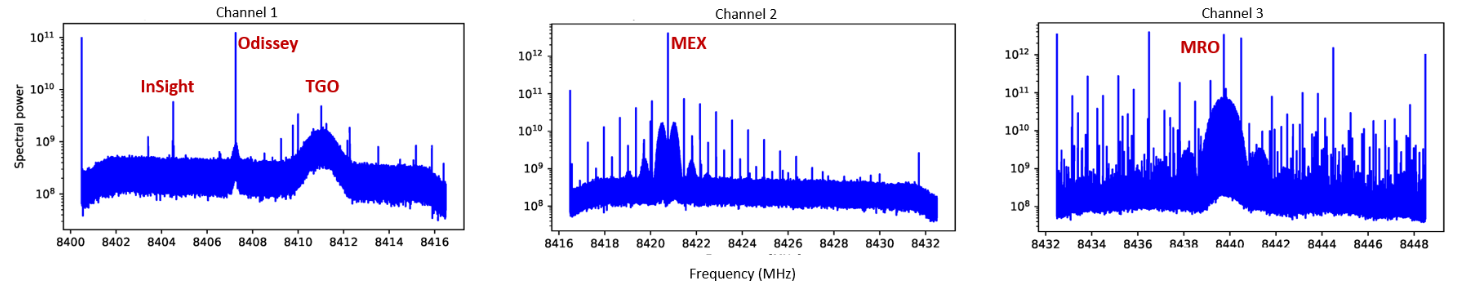
Figure 1: Simultaneous detection of the signals transmitted by several Martian orbiters and landers, from [9].
Given the synergistic nature of the JUICE and Clipper trajectories, the signals of the two spacecraft are expected to be visible in the same beam of ground-based telescopes during a significant fraction of their Jovian tours. Looking in detail at JUICE and Clipper flybys’ sequences displayed in Figure 2, the two spacecraft will occasionally perform near-simultaneous flybys around different moons, with typically only a coupled of days between JUICE’s and Clipper’s flybys. The relative angular measurements derived from PRIDE VLBI observations might then translate into direct constraints of the moons’ relative states, expected to be extremely valuable for the ephemerides solutions.

Figure 2: JUICE and Europa Clipper trajectories (altitude with respect to the moons)
Contribution of these observations to the Galilean satellites’ ephemerides
Our open-source estimation tool (Tudat(py)1) is now able to concurrently simulate several missions with different trajectories and observation schedules in a single estimation [10]. It is also linked with a VLBI prediction tool allowing to search for suitable phase calibrators close to the spacecraft at any potential observation epoch. Using these functionalities, we perform a simulation study to quantify the potential contribution of multi-spacecraft (in-beam) VLBI observations, also analysing its sensitivity to the observations’ cadence and accuracy.
To this end, we will investigate when multi-spacecraft VLBI observations could be obtained from the JUICE and Clipper spacecraft. This involves searching for suitable phase calibrators and ensuring that both spacecraft are visible from ground telescopes at a given epoch. We will also further investigate promising observation geometries (e.g. near-simultaneous flybys, see Figure 2). The simulated multi-spacecraft observables will then be added to a joint JUICE – Clipper estimation, which also includes nominal (single-spacecraft) PRIDE VLBI observations for JUICE.
We will then precisely quantify the contribution of these simulated multi-spacecraft VLBI observations to the estimation solution, focusing on the moons’ ephemerides and related dynamical parameters in particular. If proven beneficial, this will motivate the acquisition of such observations during the JUICE and Clipper missions. Additionally, our sensitivity analysis will provide direct recommendations regarding observation scheduling. If need be (i.e. particularly interesting multi-spacecraft VLBI observation but no phase calibrator in the angular vicinity of the spacecraft), this could also highlight the need to search for yet unknown calibrators in a certain region of the sky.
References
[1] Dirkx et al., Planetary and Space Science 134 (2016): 82-95.
[2] Dirkx et al., Planetary and Space Science 147 (2017): 14-27.
[3] Lainey et al., Nature Astronomy 4.11 (2020): 1053-1058.
[4] A. Magnanini et al., in preparation.
[5] Gurvits et al., European Planetary Science Congress (2013).
[6] Duev et al., Astronomy & Astrophysics 541 (2012): A43.
[7] Bocanegra-Bahamon et al., Astronomy & Astrophysics 609 (2018): A59.
[8] Fayolle et al., submitted to Planetary & Space science (under revision)
[9] Molera Calvés et al., Publications of the Astronomical Society of Australia, 38, E065
[10] Fayolle et al., EGU General Assembly (2022).
1 https://docs.tudat.space
How to cite: Fayolle, M. (M. )., Dirkx, D. (D. )., Cimo, G. (G. )., Gurvits, L. (L. I. )., Lainey, V. (V. )., Molera Calvés, G. (., Pallichadath, V. (V. )., Vermeersen, B. (L. L. A. )., and Visser, P. (P. N. A. M. ).: Contribution of simultaneous PRIDE observations of JUICE and Clipper spacecraft to the Galilean satellites’ ephemerides, Europlanet Science Congress 2022, Granada, Spain, 18–23 Sep 2022, EPSC2022-653, https://doi.org/10.5194/epsc2022-653, 2022.
Measuring the global deformation in response to periodic tidal loading belongs to the geophysical methods devised for probing the interior structure of celestial bodies. The response depends on the magnitude and frequency of loading as well as on the microphysical deformation mechanisms involved. Throughout the past ten years, it has proven useful and become popular to characterise the planet’s reaction by the Andrade rheological model (Andrade, 1910; Jackson & Faul, 2010; Castillo-Rogez et al., 2011; Efroimsky 2012a,b). The model is able to predict the correct frequency dependence of attenuation in polycrystalline solids and does not underestimate the high-frequency tidal dissipation, as it is the case with the simpler Maxwell viscoelastic model (see the discussion in, e.g., Renaud & Henning, 2018). However, the ways the Andrade model is parameterised in planetary science diverge.
Within the first parameterisation, the standard formula for the Andrade compliance used in material science (e.g., Jackson & Faul, 2010) is applied and the effect of temperature, pressure, and grain size on the response is included through pseudo-period master variable:
XB = T0 (d/dR)-m exp{-E*/R (1/T-1/TR)} exp{-V*/R (P/T-PR/TR)} (1)
A complication might occur when combining the rheological model with an outcome from thermal evolution codes: the reference parameters and the implied Arrhenian viscosity law used in equation (1) are typically different from the values considered in thermal modelling, which might lead to inconsistencies. However, when only used within the tidal framework and with a fixed interior structure, this “α-β approach” yields useful predictions and is traditionally applied in studies of terrestrial planets and the Moon (e.g., Nimmo et al., 2012; Padovan et al., 2014; Steinbrügge et al., 2018; Bagheri et al., 2019).
In the second case, a new parameter ζ is introduced (Efroimsky, 2012a), where ζ=1 corresponds to the fit to experimental data presented by Castillo-Rogez et al. (2011). The advantage of the reparameterisation is the substitution of a parameter with a fractional dimension (β) with a parameter that has a clearer physical interpretation: ζ specifically represents the ratio of the characteristic anelastic and viscoelastic deformation timescales. This approach only takes the grain size into account through the actual viscosity profile and does not require the introduction of a pseudo-period. Therefore, it can be more easily linked to the viscosity profiles outputted by thermal evolution models. The “α-ζ approach” has been considered by several studies of layered icy bodies and also applied to Venus and terrestrial exoplanets (Castillo-Rogez et al., 2011; Dumoulin et al., 2017; Tobie et al., 2019; Bolmont et al., 2020).
Here, we compare the tidal deformation and dissipation within several solar system bodies (with a special focus on Moon and Mars), calculated in the two approaches and using typical values of the parameters α, β, and ζ and viscosity laws considered in the literature. An illustration of this comparison is presented in Figure 1. We evaluate the differences in the resulting tidal parameters and endeavour to find a mapping between the global response models with constant ζ and the models with constant β that use the pseudo-period (1). The understanding of the different parameterisations, the way they are used in planetary science in combination with the thermal evolution models, and eventually the depth-dependence of the relevant variables, may provide valuable insights into the link between microphysical deformation mechanisms and the observed tidal deformation.
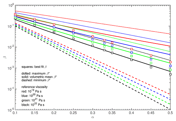
Figure 1: Preliminary comparison of the two parameterisations. Lines indicate the minimum, maximum, and volumetrically averaged value of β that would correspond to a constant (depth-independent) ζ in a layered interior model (depending on the parameter α and on the local temperature and pressure). Squares indicate the values of β which, used together with the pseudo-period (1), best fit the tidal Love number k2 calculated within the α-ζ approach with constant ζ.
References
Andrade, E. N. D. C. (1910) Proceedings of the Royal Society of London Series A, vol. 84, no. 567, pp. 1–12.
Bagheri, A., Khan, A., Al-Attar, D., Crawford, O., and Giardini, D. (2019) Journal of Geophysical Research (Planets), vol. 124, no. 11, pp. 2703–2727. doi:10.1029/2019JE006015.
Bolmont, E., Breton, S. N., Tobie, G., Dumoulin, C., Mathis, S., and Grasset, O. (2020) Astronomy and Astrophysics, vol. 644. doi:10.1051/0004-6361/202038204.
Castillo-Rogez, J. C., Efroimsky, M., and Lainey, V. (2011) Journal of Geophysical Research (Planets), vol. 116, no. E9. doi:10.1029/2010JE003664.
Dumoulin, C., Tobie, G., Verhoeven, O., Rosenblatt, P., and Rambaux, N. (2017) Journal of Geophysical Research (Planets), vol. 122, no. 6, pp. 1338–1352. doi:10.1002/2016JE005249.
Efroimsky, M. (2012a) Celestial Mechanics and Dynamical Astronomy, vol. 112, no. 3, pp. 283–330. doi:10.1007/s10569-011-9397-4.
Efroimsky, M. (2012b) The Astrophysical Journal, vol. 746, no. 2. doi:10.1088/0004-637X/746/2/150.
Jackson, I., Faul, U. H., Suetsugu, D., Bina, C., Inoue, T., and Jellinek, M. (2010) Physics of the Earth and Planetary Interiors, vol. 183, no. 1–2, pp. 151–163. doi:10.1016/j.pepi.2010.09.005.
Nimmo, F., Faul, U. H., and Garnero, E. J. (2012) Journal of Geophysical Research (Planets), vol. 117, no. E9. doi:10.1029/2012JE004160.
Padovan, S., Margot, J.-L., Hauck, S. A., Moore, W. B., and Solomon, S. C. (2014) Journal of Geophysical Research (Planets), vol. 119, no. 4, pp. 850–866. doi:10.1002/2013JE004459.
Renaud, J. P. and Henning, W. G. (2018) The Astrophysical Journal, vol. 857, no. 2. doi:10.3847/1538-4357/aab784.
Steinbrügge, G., Padovan, S., Hussmann, H., Steinke, T., Stark, A., and Oberst, J. (2018) Journal of Geophysical Research (Planets), vol. 123, no. 10, pp. 2760–2772. doi:10.1029/2018JE005569.
Tobie, G., Grasset, O., Dumoulin, C., and Mocquet, A. (2019) Astronomy and Astrophysics, vol. 630. doi:10.1051/0004-6361/201935297.
How to cite: Walterova, M., Wagner, F. W., Plesa, A.-C., and Breuer, D.: The two parameterisations of the Andrade rheological model in planetary science: a comparative study, Europlanet Science Congress 2022, Granada, Spain, 18–23 Sep 2022, EPSC2022-1102, https://doi.org/10.5194/epsc2022-1102, 2022.
Introduction
Most spacecraft missions to small bodies provide the gravity field of their targets. As the extended gravity field is an expression of the mass distribution within the body, it can provide information about its interior structure, and that in turn can constrain its origin and history.
We present a method to detect density anomalies within a small body from the global gravitational potential. As is well known, such an inverse problem is ill-posed [1], and requires regularization. Our main assumption, which mitigates the non-uniqueness of the problem, is that the interior of the body is composed of a finite number of domains, in which the density is uniform. The boundary of each domain is therefore a surface, that we describe as the level-set of a function. This approach, known as the level-set method, has been extensively used in local inversions of Earth’s gravity measurements [2]. It simplifies the manipulation of complex shapes, which in our case delimit the density anomalies.
In order to reduce the dimensionality of the problem, we employ parametric expressions for the level-set functions. The aim is then to determine the parameters of each level-set function, which describe the location and size of the anomalies, along with the density within each anomaly and the bulk density of the body.
Methods
We model the gravity field of the body through a mascons approach [3]. The observables we consider are the coefficients of the spherical harmonic expansion of the potential. By implementing a continuous approximation for the unit step function, the partials derivatives of the measurements with respect to the level-set function parameters can be computed via the chain rule [4]. Then, the function parameters and the densities can be estimated via non-linear least-squares inversion of the gravity data.
However, the problem is generally non-convex, which means that in order to converge to a global optimum the a priori values for the unknowns should be close to this solution. Since we assume no initial knowledge of the distribution to retrieve, a preliminary step is needed for the definition of an a priori model. To this end, we generate a Voronoi partition of the interior from randomly sampled points within the body. The domains are now fixed, and only the densities within each Voronoi cell are estimated from the data. This inversion problem is linear, but the solution will depend on the partition of the body. However, averaging solutions from many of such random partitions can provide a good approximation of the true model [5]. This averaged solution is then used to initialize the values of the level-set algorithm.
Discussion and outlook
We have tested the ability of our level-set implementation to retrieve interior models from simulated gravity data.
Figure 1 shows an example of the inversion results for a Bennu-shaped body. In this case, the level-set functions are chosen so that the anomalies they describe are cuboids. The model in Figure 1a is the ground truth, used to simulate gravity coefficients up to degree 11. Figure 1b shows the density retrieved from the noise-free data, and Figure 1c the results when the data are perturbed by 1% Gaussian noise. The method can retrieve the location and density of the anomalies with good approximation, even in the perturbed case. For anomalies where the density and the size cannot be estimated simultaneously, such as with nearly-spherical shapes, the method can usually still correctly determine the total mass and the position of the center-of-mass. The size could then be constrained by independent observations from other instruments or by theoretical models.
In a more realistic scenario, the resolution of the gravity would be lower, and the noise profile would be increasing with the degree of gravity. This could aggravate the non-uniqueness problem, since having fewer and less precise measurements could lead to different models fitting the data equally well. Current work is focused on improving the robustness of our approach and on better defining its limitations in its application to real gravity measurements.
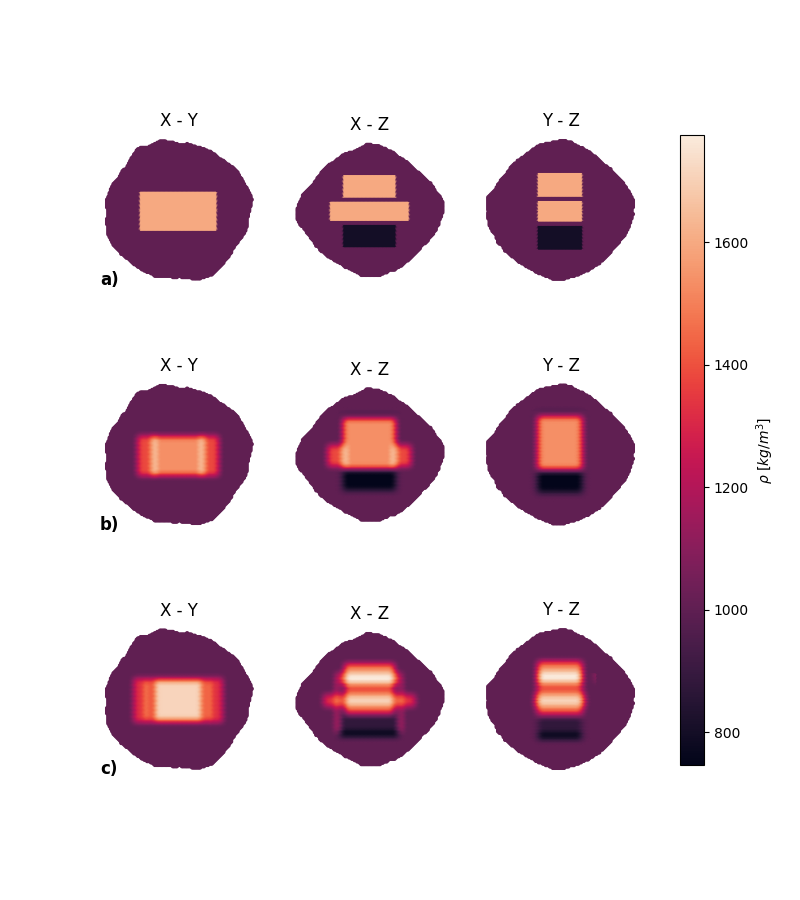
Figure 1. Interior density models, shown via sections along 3 planes perpendicular to the body axes and containing the origin: a) Ground truth; b) Solution from noise-free data; c) Solution from data with 1% noise
Acknowledgements
This work was financially supported by the French community of Belgium within the framework of a FRIA grant, and by the Belgian PRODEX program, managed by the European Space Agency in collaboration with the Belgian Federal Science Policy Office.
References
[1] V. Isakov. Inverse Source Problems. American Mathematical Soc., 1990.
[2] J. Giraud, M. Lindsay, and M. Jessell. Generalization of level-set inversion to an arbitrary number of geologic units in a regularized least-squares framework. GEOPHYSICS, 86(4):R623–R637, July 2021.
[3] S. Le Maistre, A. Rivoldini, and P. Rosenblatt. Signature of Phobos’ interior structure in its gravity field and libration. Icarus, 321:272–290, March 2019.
[4] A. Aghasi, M. Kilmer, and E. L. Miller. Parametric Level Set Methods for Inverse Problems. SIAM Journal on Imaging Sciences, 4(2):618–650, January 2011.
[5] L.-I. Sorsa, M. Takala, P. Bambach, et al. Tomographic inversion of gravity gradient field for a synthetic Itokawa model. Icarus, 336:113425, January 2020.
How to cite: Caldiero, A., Le Maistre, S., and Dehant, V.: A parametric level-set approach to the global gravity inversion of small bodies, Europlanet Science Congress 2022, Granada, Spain, 18–23 Sep 2022, EPSC2022-1118, https://doi.org/10.5194/epsc2022-1118, 2022.
Please decide on your access
Please use the buttons below to download the presentation materials or to visit the external website where the presentation is linked. Regarding the external link, please note that Copernicus Meetings cannot accept any liability for the content and the website you will visit.
Forward to presentation link
You are going to open an external link to the presentation as indicated by the authors. Copernicus Meetings cannot accept any liability for the content and the website you will visit.
We are sorry, but presentations are only available for users who registered for the conference. Thank you.
Please decide on your access
Please use the buttons below to download the presentation materials or to visit the external website where the presentation is linked. Regarding the external link, please note that Copernicus Meetings cannot accept any liability for the content and the website you will visit.
Forward to session asset
You are going to open an external link to the asset as indicated by the session. Copernicus Meetings cannot accept any liability for the content and the website you will visit.
We are sorry, but presentations are only available for users who registered for the conference. Thank you.