Multiple terms: term1 term2
red apples
returns results with all terms like:
Fructose levels in red and green apples
Precise match in quotes: "term1 term2"
"red apples"
returns results matching exactly like:
Anthocyanin biosynthesis in red apples
Exclude a term with -: term1 -term2
apples -red
returns results containing apples but not red:
Malic acid in green apples
hits for "" in
Network problems
Server timeout
Invalid search term
Too many requests
MITM4
Session assets
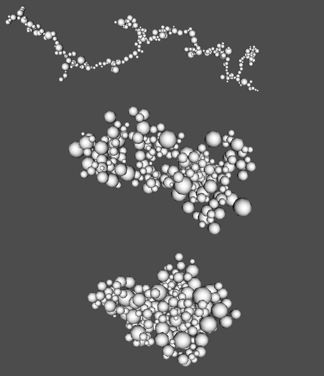
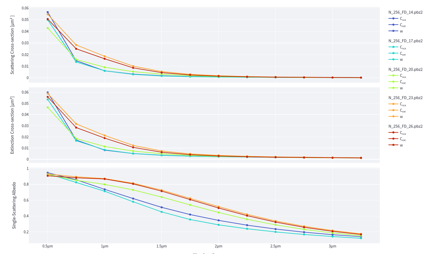
How to cite: Arnaut, M., Schauten, D., Nagel, C., and Wöhler, C.: Investigating Polarimetric Effects with Fractal Clusters of Nano-Phase Iron Particles in Space Weathering, Europlanet Science Congress 2024, Berlin, Germany, 8–13 Sep 2024, EPSC2024-1034, https://doi.org/10.5194/epsc2024-1034, 2024.
Introduction
The next generation of lidar instruments will encompass the travel time measurement for each photon packet that would be available to characterize the planetary surface medium, either spaceborne, in-situ or in the lab. For instance, the BepiColombo laser altimeter (BELA) (Thomas et al., 2021) includes this capability to explore the hermian surface. We propose here a tool to simulate in-silico the time transfer inside the planetary medium.
Methods
We propose a Monte Carlo approach based on the work from Farrell et al., 1992 and Boas et al., 2002. Our model computes the position of the ray during its travel through the medium. The main parameters are incidence angle, the optical thickness, the single scattering albedo, the Henyey-Greenstein or isotropic phase function.
Validation
The validation of the model is a mandatory step in order to compute a coherent and physically correct simulation of light time transfer within a planetary surface medium. In the model, planetary surface mediums can be either described as a semi-infinite granular layer or a homogeneous slab above a bedrock with a certain albedo. The purpose here is to be able to replicate the same simulations in the same conditions from previous works such as Gao et al., 2013 , Gautheron et al., 2024 and Patterson et al., 1989. We first computed the reflectance in the same conditions as seen in Gao et al., 2013 in the case of a semi-infinite granular layer (Figure 1) which are an incidence angle of 50 degree, an optical thickness of 1000 and an isotropic phase function. The DISORT algorithm (Stamnes et al., 1998) gives a numerical solution for this case that is also computed and displayed for a double check. By comparing both DISORT solutions and Gao et al., 2013 results, our simulation shows a very good agreement, confirming the validity of our model in terms of angular distribution.
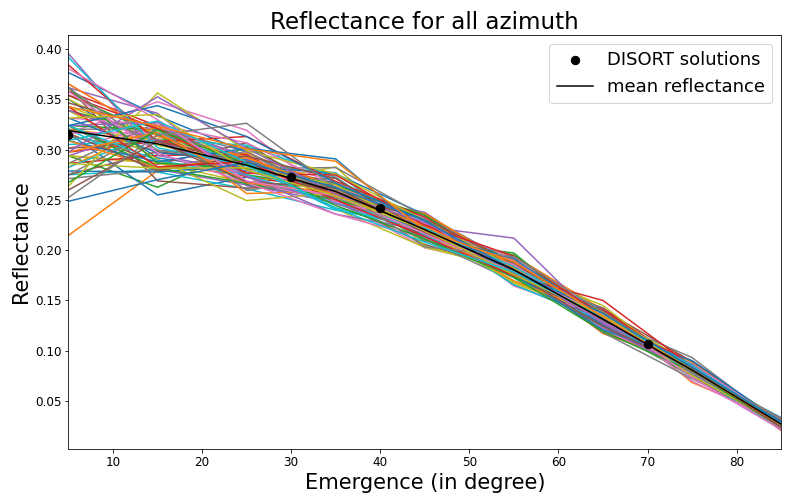
Figure 1 : Reflectance for all azimuth computed in the conditions of semi-infinite granular layer for an incidence of 50 degrees,single scattering albedo omega = 1. Scattered rays follow isotropic diffusion law as expected ; black dots represents the DISORT solution ; black line represents the mean reflectance value for all azimuth ; color lines represents reflectance following the emergence for different azimuth
We propose then a method to compute the trajectory and the time travel of the rays in the medium, that would be simulating the response of a full waveform lidar. Knowing the speed of light in the medium and assuming its constancy according to the medium’s optical properties, we then evaluate the time travel in comparison with the analytical solution from Patterson et al., 1989. Results in Figure 2 shows a very good agreement that validates our algorithm.

Figure 2 : Histogram of time travel for an instance of semi-infinite granular layer compared with the analytical solution from Patterson et al., 1989. Here the source of the rays is isotropic at a depth z0 and observed at a distance 10 mm. The absorption coefficient is 0.005 mm-1, the scattering coefficient is 1 mm-1 and the speed of light is 299792458 m/s.
Result
As an illustration of the capabilities of our tool, we computed the travel time in the following conditions : an input incidence of 0°, a sufficient optical thickness to reach semi-infinite layer conditions and a Henyey-Greenstein phase function ; Figure 3 illustrates this situation. We can observe that most of the photons reach the surface in a short period of time meaning their travel length is rather small. Between 0.4 ns and 1 ns, fewer photons reach the surface implying a longer travel length. Thus, we are now able to discuss how the media properties will affect the response of a full waveform lidar.

Figure 3: Histogram of travel time from an input of 1 million rays, incidence = 0° with omega = 0.99 and a Henyey-Greenstein phase function with a scattering anisotropy of g = 0.8 , tau = 60 (semi-infinite medium). The absorption coefficient is 0.005 mm-1, the scattering coefficient is 1 mm-1 and the speed of light is 299792458 m/s.
Conclusion and perspectives
We propose a new approach to efficiently simulate the travel time of photons inside a planetary surface. We conducted several tests to validate the approach and one simulation in realistic condition. In the future, we will adapt this tool to peculiar planetary science cases, such as the mercury regolith for BELA, or the icy surface for GALA.
References
Boas, D. A., J. P. Culver, J. J. Stott, and A. K. Dunn, "Three dimensional Monte Carlo code for photon migration through complex heterogeneous media including the adult human head," Opt. Express 10, 159-170 (2002)
Farrell, T.J., Patterson, M.S. and Wilson, B. (1992), A diffusion theory model of spatially resolved, steady-state diffuse reflectance for the noninvasive determination of tissue optical properties in vivo. Med. Phys., 19: 879-888. https://doi.org/10.1118/1.596777
Gao, M., X. Huang, P. Yang, and G. W. Kattawar, "Angular distribution of diffuse reflectance from incoherent multiple scattering in turbid media," Appl. Opt. 52, 5869-5879 (2013)
Gautheron Arthur, Raphaël Clerc, Vincent Duveiller, Lionel Simonot, Bruno Montcel, and Mathieu Hébert, "On the validity of two-flux and four-flux models for light scattering in translucent layers: angular distribution of internally reflected light at the interfaces," Opt. Express 32, 9042-9060 (2024)
Patterson, M. S., B. Chance, and B. C. Wilson, "Time resolved reflectance and transmittance for the noninvasive measurement of tissue optical properties," Appl. Opt. 28, 2331-2336 (1989)
Stamnes, K.; Tsay, S.-C.; Jayaweera, K. & Wiscombe, W. Numerically stable algorithm for discrete-ordinate-method radiative transfer in multiple scattering and emitting layered media Appl. Opt., 1988, 27, 2502-2509, http://dx.doi.org/10.1364/AO.27.002502
Thomas, Nicolas & Hussmann, Hauke & Spohn, Tilman & Lara, L. & Christensen, Ulrich & Affolter, Michael & Bandy, T. & Beck, T. & Chakraborty, S. & Geissbuehler, U. & Gerber, Michael & Ghose, K. & Gouman, J. & Hosseiniarani, Alireza & Kuske, K. & Peteut, A. & Piazza, Daniele & Rieder, M. & Servonet, A. & Metz, Bodo. (2021). The BepiColombo Laser Altimeter. Space Science Reviews. 217. 10.1007/s11214-021-00794-y.
How to cite: Barron, J., Schmidt, F., and Andrieu, F.: Radiative transfer and travel time to characterize the surface, Europlanet Science Congress 2024, Berlin, Germany, 8–13 Sep 2024, EPSC2024-930, https://doi.org/10.5194/epsc2024-930, 2024.
Range resolution is one of the key performance metrics for a radar instrument. It is driven by the time resolution of its soundings, and the electromagnetic properties of the sounded material. This resolution is set by design, as it is limited by the bandwidth of the instrument: the larger the bandwidth, the better the resolution. Modern radar modulation techniques require a spectral estimation method to obtain a time-domain signal for human-interpretation. The Fast Fourier Transform is generally selected for its robustness and efficiency. However, the time resolution of this method is limited by the inverse of the bandwidth, and the necessary windowing for side-lobes reduction. For this reason, « super-resolution » techniques have been introduced in the 1980s, based on parametric signal models [6].
The « Bandwidth Extrapolation » (BWE) techniques [2] fit a parametric model to a measured radar signal’s spectrum. This spectrum is then extrapolated forward and backward to increase the bandwidth, and the spectrum is eventually Fourier transformed to obtain a sounding in time-domain. The resolution enhancement compared to the FFT (without windowing) is equal to the extrapolation factor. This extrapolation is possible because a measured radar spectrum can be modelled by a sum of complex sine-waves with different amplitudes, frequencies and phases. Each of the complex sine-waves corresponds to an echo in time-domain. In practical cases, this deterministic signal is corrupted by various sources of noise, distorsions, and can be dampened by losses in the sounded material. Hence a limitation of the extrapolation by a factor of 3 [8].
Invented for Earth radars, this technique has been extensively applied to planetary radar sounders in the last decade, allowing futher insights on the sub-surface structure and composition of the Moon, Mars and Titan. Results of the BWE applied to planetary radar studies include: (1) the first bathymetry of a Titan sea (Cassini mission [7]), (2) the stratigraphic analysis of the Martian polar ice sheet (Mars Express [5] and MRO missions [12]), (3) the estimation of the Martian shallow sub-surface attenuations (Mars 2020 mission [4]), (4) the preparation of future Martian drilling operations (ExoMars mission [9]).
We released this year the first open-source BWE software, as a Python library named « PyBWE » [10]. PyBWE is accessible on PyPI, and the source code on GitHub. It is divided into 3 packages, corresponding to 3 different signal models for bandwidth extrapolation:
- PyBWE: the « classic » BWE technique [2], currently the only one applied to planetary radar data, with an AR model determined using the Burg algorithm.
- PyPBWE: the « Polarimetric BWE » technique [13], adapted to radars with multiple polarimetric configurations, with a multi-channel AR model determined using a multi-channel Burg algorithm.
- PySSBWE: the « State-Space BWE » technique [11], more robust to noise and signal attenuations, with an ARMA model determined using a State-Space modelling approach.
We intend this library to be useful for both radar experts and non-radar experts within the planetary science community. For this reason, each package proposes integrated solutions, as well as individual functions for modelling and extrapolation. Are included in PyBWE: an exhaustive documentation, example scripts and automated performance tests.
Results from one of the examples provided with PyBWE for the PySSBWE package is presented in frequency-domain in Fig. 1, as an illustration of the capability of the method to reconstruct a radar spectrum in the presence of attenuations and a high level of white noise.
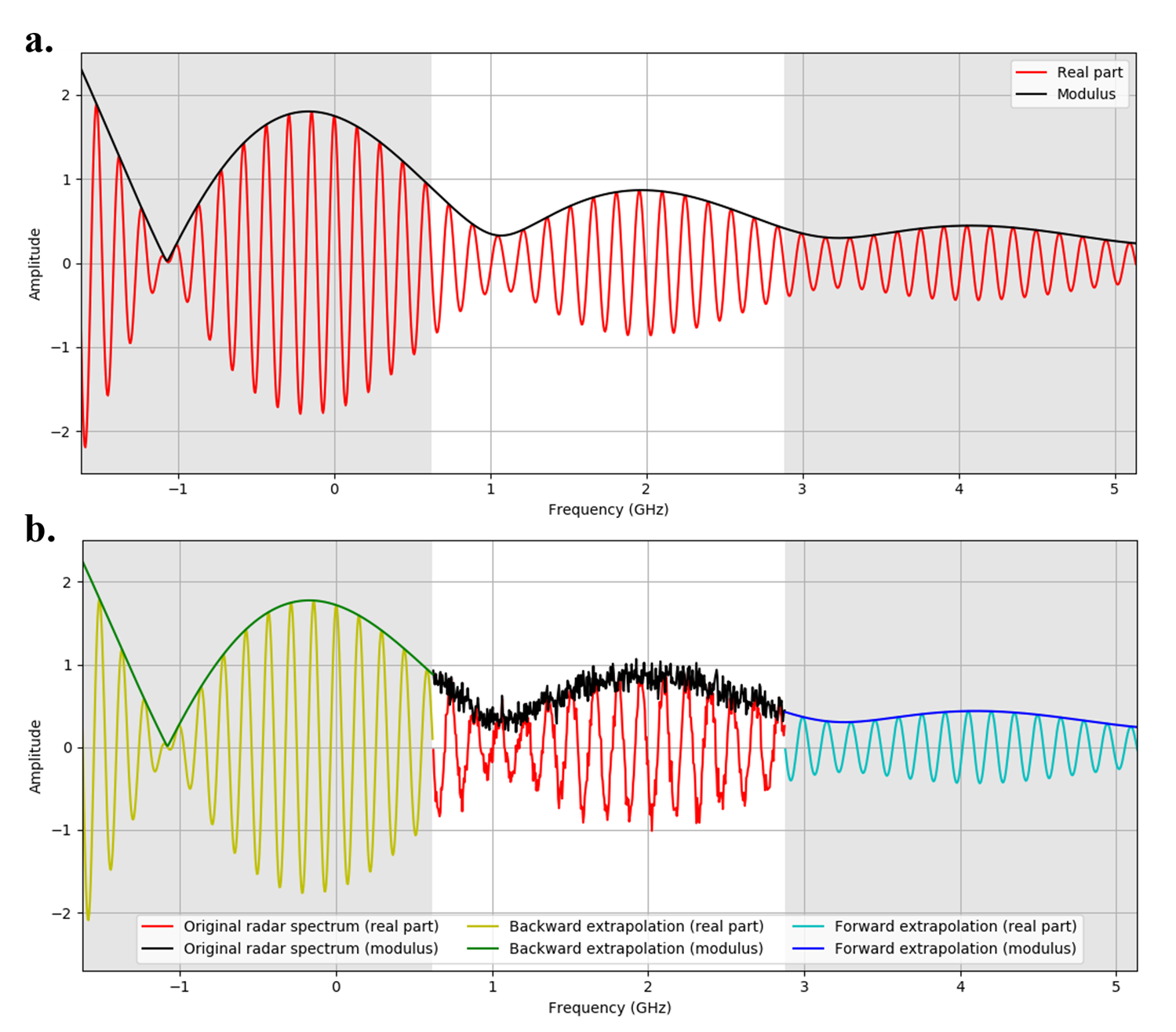
Fig. 1 Example of application of the PySSBWE package on a synthetic radar spectrum, generated for 2 complex sinusoids of amplitudes 1 and 0.75, with exponential frequency domain decays 0.25 and 0.5 GHz-1, corresponding to targets at 1 and 1.07 m from the antennas. The signal is corrupted by a white Gaussian noise of std 0.1. The original bandwidth is 0.5-3 GHz, corresponding to the working frequencies of the WISDOM radar (ExoMars mission [1]) (a) Expected spectrum after extrapolation in the absence of noise, for comparison (b) Spectrum extrapolated forward and backward with PySSBWE
Applications of PyBWE to the WISDOM (ExoMars mission), RIMFAX (Mars 2020 mission) and RoSPR (Tianwen-1 mission) radars will be proposed to illustrate this work. See Fig. 2 for an example on an experimental WISDOM radargram [1]. With the selection of radar sounders for the exploration of Venus (EnVision mission) and Jupiter’s icy moons (JUICE and Europa Clipper missions), we expect PyBWE to have many applications in the future. In addition, we plan to maintain and update the library, and the recent developments in super-resolution techniques [3] could be integrated as new packages.
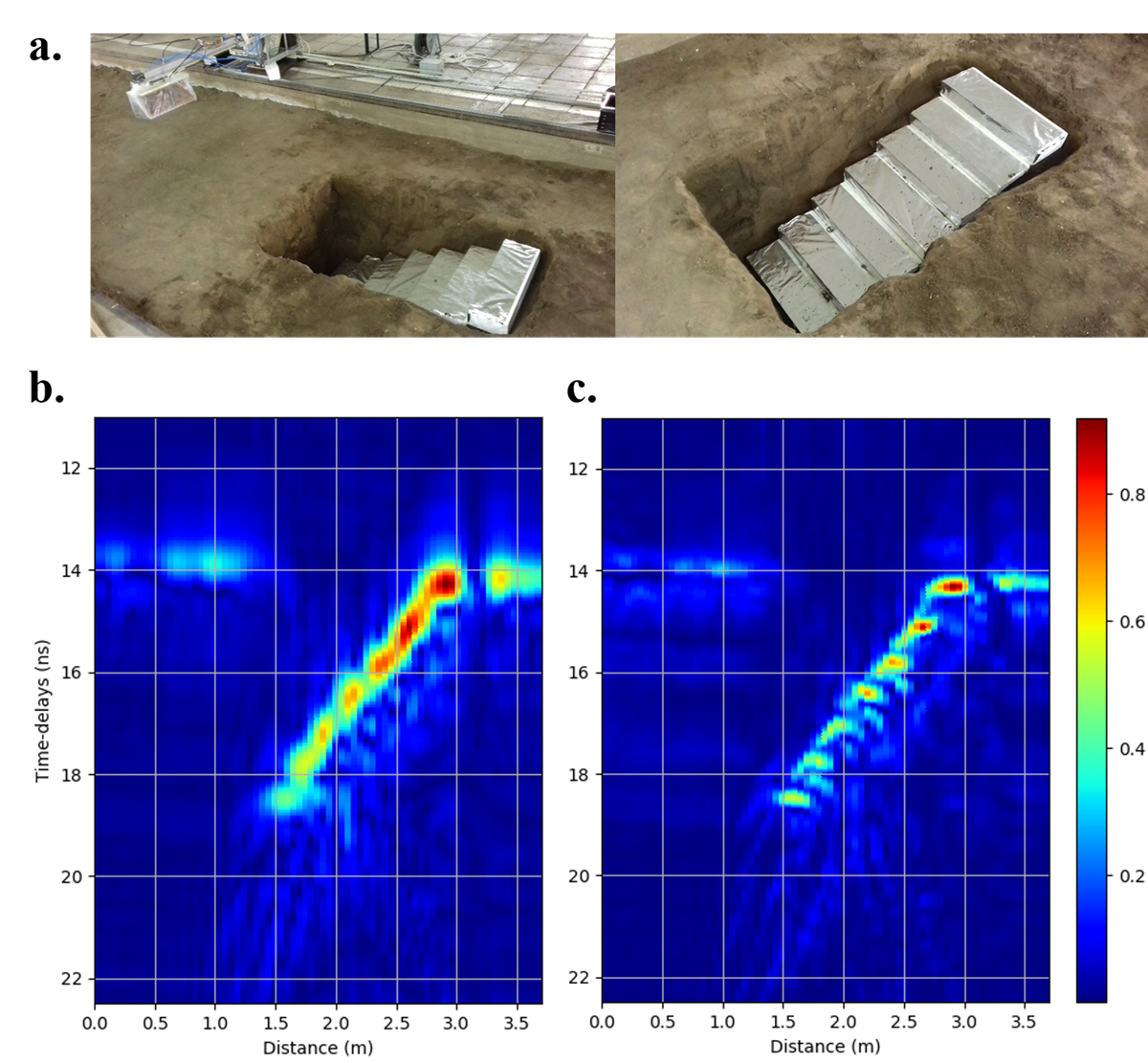
Fig. 2 Application of PyBWE to an experimental WISDOM (ExoMars mission [1]) radargram acquired during a measurement campaign on Earth (a) Experimental set-up with a metallic staircase below a flight model of the WISDOM instrument, each step being separated by a 10 cm height (b) Radagram obtained after a classic IFFT and Hamming windowing, where the different steps cannot clearly be separated (c) Radargram obtained after BWE, where the different steps are now resolved
References:
[1] Ciarletti et al., 2017, Astrobiology, https://doi.org/10.1089/ast.2016.1532
[2] Cuomo, 1992, Lincoln Laboratory report
[3] Donini et al., 2024, IEEE Transactions on Geoscience and Remote Sensing, https://doi.org/10.1109/TGRS.2024.3378576
[4] Eide et al., 2022, Geophysical Research Letters, https://doi.org/10.1029/2022gl101429
[5] Gambacorta et al., 2022, IEEE Transactions on Geoscience and Remote Sensing, https://doi.org/10.1109/tgrs.2022.3216893
[6] Kay & Marple, 1981, Proceedings of the IEEE https://doi.org/10.1109/proc.1981.12184
[7] Mastrogiuseppe et al., 2014, The bathymetry of a titan sea, Geophysical Research Letters, https://doi.org/10.1002/2013gl058618
[8] Moore et al., 1997, Lincoln Laboratory Journal
[9] Oudart et al., 2021, Planetary & Space Science, https://doi.org/10.1016/j.pss.2021.105173
[10] Oudart et al., 2024 (in review), Journal of Open Source Software
[11] Piou, 1999, Lincoln Laboratory report
[12] Raguso et al., 2023, Icarus, https://doi.org/10.1016/j.icarus.2023.115803
[13] Suwa & Iwamoto, 2007, IEEE Transactions on Geoscience and Remote Sensing, https://doi.org/10.1109/tgrs.2006.885406
How to cite: Oudart, N., Ciarletti, V., Le Gall, A., and Brighi, E.: PyBWE: Open-Source Python tools for Super-Resolution applied to Planetary Radar Soundings, Europlanet Science Congress 2024, Berlin, Germany, 8–13 Sep 2024, EPSC2024-170, https://doi.org/10.5194/epsc2024-170, 2024.
Introduction
Every planetary exploration study faces a common challenge: integrating images from diverse sources, each one with unique spatial and spectral resolutions, and often, georeferencing inaccuracies. This paper presents the developments of a software suite dedicated to facilitating the integration of surface images of planetary bodies through simplified co-registration procedures and reciprocal resolution enhancement using pansharpening techniques.
The study delves into the adopted methodologies, providing a comprehensive performance analysis of the tools. We also demonstrate the practical application of the software suite in real Mars and Mercury data case studies, underscoring its potential in the field. The software will be made available open source for the benefit of the scientific community.
Automatic alignment
Accurate ground data alignment is typically adopted for surface studies and is necessary for applications like mosaicking, mapping, and photogrammetry. Despite being a common need, data registration remains a process approached manually: the operator searches for matching features within the images in a Geographic Information System (GIS) and decides the function to align based on experience, trial and error, and software availability. This procedure is time-consuming and greatly influenced by the user's skill and perseverance.
Our current research presents an alternative approach using an automatic alignment methodology we developed based on the Scale-invariant feature transform (SIFT) computer vision algorithm [1], a powerful tool inherited from the photogrammetric and computer vision fields. This algorithm can identify significantly more tie points (matching features between images) than a human operator, and in a fraction of the time (Fig.1). Subsequently, matching points are used in two distinct phases: (i) an initial pre-alignment through a homographic transformation, which allows the general geometry of the images to be matched, and (ii) a refinement phase, which allows local features outside the general topography to be taken into account, operated by software or manually. This procedure considerably reduces co-registration time and permits the achievement of up to pixel-level accuracy across the whole image.
Pansharpening
Beyond the necessity, integrating different data allows for the mutual improvement of information. In this sense, the pansharpening family of methods represents one of the most discussed and established disciplines in remote sensing. Pansharpening refers to the fusion of the spectral properties of a multi/hyperspectral cube with a higher spatial resolution panchromatic image. In this way, the resulting data will possess high spatial and spectral resolution, gaining the advantages and capabilities of both sources simultaneously.
Despite the succession of techniques over more than forty years of development [2], the difficult alignment and the lack of accessible tools have meant that pansharpening has rarely been used in planetary sciences outside the Earth Observation field. Among the few examples, pansharpening has proven appreciable advantages for morphological analysis [3, 4] and image simulation [5].
Our developments make it possible to apply different component substitution (CS) pansharpening techniques suitable for different fields of application and purposes.
The pixel-wise CS methods are generally considered the most traditional and well-established. Although early applications have been considered to suffer from alteration in the spectral response and its slope, more recent techniques display that this problem is now commonly minimised [6, 7].
Validation and case studies
Our suite is not dedicated to a single instrument or condition but is fit for use with images from different sources and with different resolution ranges. A large dataset was adopted for validation, including data from the ExoMars TGO CaSSIS, Mars Reconnaissance Orbiter HiRISE, CTX and CRISM, and Mars Express HRSC instruments on Mars observation, and Messenger MDIS NAC and WAC on Mercury. Furthermore, the chosen images range in lighting conditions, surface geological properties and acquisition geometry, allowing the influence of these factors to be observed (Fig,2).
During testing, spatial resolution increases of up to sixteen times the original were probed, specifically between the colour bands of CaSSIS (4.5 m/px) and the RED band of HiRISE (0.25 m/px) (Fig,3. The results were then analysed using various numerical performance indicators and a visual survey. The evaluation indexes adopted include SAM, RMSE, ERGAS, UQI, PSNR, and SSIM, which are suitable for verifying the resulting images' spectral and structural properties.
Acknowledgements
The study is part of the INAF MiniGrant “Combined implementation of CaSSIS and HiRISE data through pansharpening experiments” (CUP C93C23008430001) and it has also been supported by the Italian Space Agency (ASI-INAF agreement no. 525 2017- 03-17).
References
[1] Lowe, D. G. (1999). IEEE Int. Conf. Comput. Vis., 1150–1157 vol.2.
[2] Vivone, G., et al. (2021). IEEE Geosci. Remote Sens. Mag., 9(1), 53–81.
[3] Kwan, C., et al. (2017). IEEE Int. Geosci. Remote Sens. Symp. (IGARSS).
[4] Semenzato, A., et al. (2020). Remote Sens., 12(19), 3213.
[5] Tornabene, L. L., et al. (2017). Space Sci. Rev., 214(1).
[6] Aiazzi, B., et al. (2007). IEEE Trans. Geosci. Remote Sens., 45(10), 3230–3239.
[7] Palubinskas, G. (2013). J. Appl. Remote Sens., 7(1), 073526.
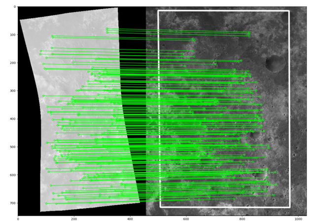
Fig. 1 Example of CRISM image (on the left) aligned to a reference HRSC image on the right) through matching points between images (linked in green) acquired by SIFT operator.
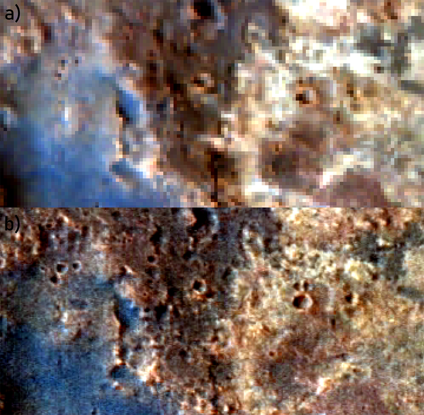
Fig. 2 Example of augmentation of a (a) hyperspectral cube (CRISM hrl00004962_07_sr183j_mtr3). The resulting image (b) shows three times the original resolution when combined with HRSC using a MMSE Brovey implementation.
Fig. 3 Detail of the maximum resolution increase obtained during testing, from 4.5 m/px (a) CaSSIS mosaic MY34_004209_158_0 – RPB) to 0.25 m/px (b) with PSP_010394_2025 HiRISE by Gram-Schmidt pansharpening algorithm.
How to cite: Tullo, A., Re, C., Martellato, E., La Grassa, R., Vergara, N. A., Simioni, E., Cambianica, P., Munaretto, G., and Cremonese, G.: On the road to an open-source co-registration and pansharpening suite for planetary sciences: Developments and case studies, Europlanet Science Congress 2024, Berlin, Germany, 8–13 Sep 2024, EPSC2024-527, https://doi.org/10.5194/epsc2024-527, 2024.
On 26 September 2022, NASA’s Double Asteroid Redirection Test (DART) mission impacted Dimorphos, the moonlet of near-earth asteroid 65803 Didymos, performing the world’s first planetary defence test. ESA’s Hera mission will be launched in October 2024 and rendezvous with the Didymos system end of 2026 or beginning of 2027. It will closely investigate the system and in particular the consequences of the DART impact.
Hera carries the hyperspectral imager Hyperscout-H. Its sensor consists of 2048 × 1088 pixels which are arranged in macro pixel blocks of 5 × 5 pixels. The 25 pixels of each block are covered with filters in 25 different wavelengths where the center response ranges from 657 to 949 nm. Therefore, each of the 2048 × 1088 pixels provides only the brightness information for one wavelength and hence the theoretical 2048 × 1088 × 25 data cube is only sparsely populated.
A simple straight forward approach to replenish the sparse data cube would be to move a 5 × 5 pixel window with one pixel steps horizotally and vertically over the whole frame and assign the obtained 25 wavelength spectrum to the center pixel of the window. Besides reducing the image resolution to the quite coarse macro pixels, the accuracy of this method is limited by pixel to pixel variations of the spectra and even more by varying albedo and shading effects caused by varying surface inclination. This makes the resultant spectra very noisy.
In order to retrieve more accurate spectra with higher spatial resolution, we separate the spectrum at each micro pixel into a normalized spectrum and a brightness scaling factor. We assume the normalized spectra to be spatially smooth, but not necessarily the scaled spectra. Ratios of measured values are used to iteratively compute the normalized spectral value from adjacent pixels. After convergence, the normalized spectra are brightness scaled to reproduce the measured values. This approach, which we call de2, allows to replenish the complete data cube with full micro pixel resolution. The application to simulated test images shows that spectra are recovered much more accurately than with the direct approach and that only very little spatial detail is lost. An example spectrum for a simulated Hyperscout-H image based on data of asteroid 25143 Itokawa acquired by the Multi-band Imaging Camera (AMICA) aboard the Hayabusa spacecraft is shown in the image below.

The green line is the true (the simulated) spectrtum, the blue line is the simple direct approach, and the red line is our de2 approach.
The spectra of atmosphereless solar system bodies generally display broad absorption features across the visible to near-infrared wavelengths. The spectra are relatively smooth with no sharp absorption or emission lines. Therefore, it should be possible to find a low dimensional representation that preserves most of the information in the spectra. Such a low dimensional representation enables a concise visualization of the full data cubes, e.g., through false color images.
For the estimation of a low dimensional representation of spectra, we employ layered feed forward neural networks with backpropagation learning. These neural networks have an input layer and several processing layers of neurons. The last layer of neurons forms the output layer. Such neural networks are commonly used for supervised learning. This would require a large data set of spectra accompanied with classifications given by a few parameters. These data would be used to train the neural network to reproduce these classifications. Subsequently, the neural network should be able to perform the classification of new yet unclassified spectra. However, we do not have a large data set of classified spectra and simulating it appropriately may be quite difficult considering the unique reshaping process that the dart impact may have caused. After such recent reshaping, Dimorphos may be substantially different from any solar system body visited by spacecraft so far.
Therefore, we use a different approach and set up the layered neural network for unsupervised learning. We apply the same spectrum as input and as desired output of the neural network. The neural network has one layer with a small number of neurons, so it is forced to find a low dimensional representation of the input spectrum, the so-called latent dimensions, from which it can completely reconstruct the spectrum. The image below shows an example of such a neural network.
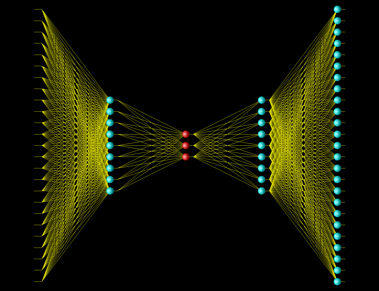
The network has four layers of neurons plus the input layer. Input and output layers have 25 dimensions, like our spectra. In the center there is a layer of only three neurons shown in red. This is the bottle neck through which the neural network has to convey the information in the spectra. The output values of these three neurons provide a low dimensional representation of the spectra, the latent dimensions. We show the results for the simulated Hyperscout-H image based on Itokawa data.
How to cite: Grieger, B., de León, J., Goldberg, H., Kohout, T., Kovács, G., Küppers, M., Nagy, B. V., Popescu, M., and Prodan, G.: Low dimensional representations of spectra from the Hyperscout-H hyperspectral imager aboard the Hera mission with artificial neural networks, Europlanet Science Congress 2024, Berlin, Germany, 8–13 Sep 2024, EPSC2024-506, https://doi.org/10.5194/epsc2024-506, 2024.
Remote sensing of the Earth and other planets of the Solar System return huge volumes of data. Retrieving information of interest from such data may consist of inverting a direct or forward physical model, which theoretically describes how parameters of interest x ∈ X are translated into observations y ∈ Y. The observations y are high-dimensional (of dimension D) because they represent signals in time, angles or wavelengths. Besides, many such high-dimensional observations are available and the application requires a very large number of inversions (denoted by Nobs in what follows). The parameters x to be predicted (of dimension L) is itself multi-dimensional with correlated dimensions. In [1] a statistical method is put forward with a Bayesian and machine learning framework capable of solving the problem of inverting physical models on multi-dimensional data in order to estimate the value of their parameters. The method addresses: 1) the large number of observations to be analysed, 2) their high dimension, 3) the need to provide predictions for several correlated parameters, 4) the possible existence of multiple solutions and 5) the requirement to provide the latter with a confidence measure (e.g. uncertainty quantification).
Here our science case consists of analysing hyperspectral images acquired in the visible and infrared at different angles over regions of interest at the surface of Mars. The interpretation of the BRDF (Bidirectional Reflectance Distribution Function) extracted from such multi-angular observations in terms of microtexture of surface materials such as grain size, shape, roughness and internal structure, which can be used as tracers of geological processes, is based on the inversion of physical models of radiative transfer (Hapke and Shkuratov models). The latter link in a nonlinear way physical and observable parameters (functional y = F(x)). In this case y = yobs is a vector of D reflectance values for D geometries (up to a few tens), x is vector of L = 4 or L = 6 photometric parameters, while the number of observations to be inverted Nobs can be of the order of a few millions. This great number of observations Nobs, organized in data cubes, results from the combination of spectral and spatial sampling of the scene. From an experimental vector yobs of reflectance values, the objective is to estimate the mean or the most probable value(s) for each of the L parameters (the components of vector x) of the physical model F and to provide a measurement of uncertainty about the estimations. Our pipeline performs the estimation in four steps:
1. The generation of a database of N couples DN = {(xn,yn), n = 1 : N} using the direct physical model, y = F(x). More specifically, xn values are simulated from a chosen prior distribution, e.g. uniform over the parameter range, and the direct model F is applied to produce F(xn) to which a typically Gaussian noise is added to provide yn. F is supposed to be available as a closed-form expression.
2. The learning phase in which the pipeline constructs from the database a direct and an inverse parametric statistical model of the functional y = F(x). The learned model is a Gaussian mixture model with a structured parameterization referred to as GLLiM for Gaussian Locally Linear Mapping (see [1] for details). Because it is trained on the data from step 1, it depends on the physical direct model. The inverse model is then approximated by a surrogate probability distribution function (PDF) expression pGLLiM which is learned once, for all possible yobs to be inverted, p(xy) ≈ pGLLiM(xy) .
3. This surrogate model is then used for all vectors yobs in order to build a set of a PDFs pGLLiM(xyobs).
4. The PDFs are then exploited each independently by different techniques to estimate the solution x̂ corresponding to each vector yobs: estimation by the mean/mode of the PDF, fusion of the components of the Gaussian mixture model into a small number of centroids (usually two or three) to identify possible multiple modes (we consider up to 2 modes in the following), importance sampling of the true target PDF p(xyobs) with the proposal distribution set to pGLLiM(xyobs) around the mean or around the centroids/modes, [1] to improve the quality of the predictions (eg. posterior mean, modes and variance).
The pipeline is implemented into a high-performance, documented, and open-source software PlanetGLLiM* that is specifically tailored to handle inversions of reflectance models given cubes of multi-spectral data and geometries typically produced by planetary remote sensing. PlanetGLLiM offers an easy to use graphical user interface and implements the Hapke and the Shkuratov models. Custom models can be added by the user in the form of a single Python class. The PlanetGLLiM application played a crucial role in conducting the first large-scale inversion of a dataset derived from multi-angular observations across various type localities on Mars using the CRISM sensor [2], enabling their spectrophotometric and physical characterization. The method was also applied to perform a massive Hapke model inversion on Pleiades satellite data to map the physical properties of the Moon surface [3].
* https://kernelo-mistis.gitlabpages.inria.fr/planet-gllim-front-end/
[1] B. Kugler, F. Forbes, and S. Douté. Fast Bayesian inversion for high dimensional inverse problems. Statistics and Computing, 32(2):31.
[2] S. Douté. In LPI Contributions, volume 3040 of LPI Contributions, page 2149, March 2024
[3] D. T. Nguyen, S. Jacquemoud, A. Lucas, S. Douté, C. Ferrari, S. Coustance, S. Marcq, and A. Meygret. In LPI Contributions, volume 3040 of LPI Contributions, page 1998, March 2024.
How to cite: Douté, S., Forbes, F., Borkowski, S., Meyer, L., and Heidmann, S.: Massive analysis of multi-angular images by inverse regression of reflectance models for the physical characterization of planetary surfaces., Europlanet Science Congress 2024, Berlin, Germany, 8–13 Sep 2024, EPSC2024-535, https://doi.org/10.5194/epsc2024-535, 2024.
Ubiquitous phyllosilicates and carbonates in Ceres’ surface regolith reveal extensive water-rock interaction in the past [1]. A key area of continued study is the water ice content of the crust and how it is mixed with regolith or salt. Nuclear spectroscopy data suggest an ice table may be buried just within a few mm from the surface, gradually receding to larger depths toward the equator due to increasing solar insolation [2]. On the other hand, a global inventory of ice-related morphological features points to a heterogeneous distribution of ice in the subsurface and a relatively low ice content (< 50 vol%) [3]. Gravity data places even a more conservative constraint on Ceres’ crustal ice (< 25 vol%), necessitating stronger phases such as hydrated salts (≥ 36 vol%) to account for the observed topography [4, 5]. Ice has been spectroscopically detected in 9 fresh craters [6] where it was likely excavated by impacts. This offers a window into Ceres’ shallow subsurface and the nature of ice in its crust.
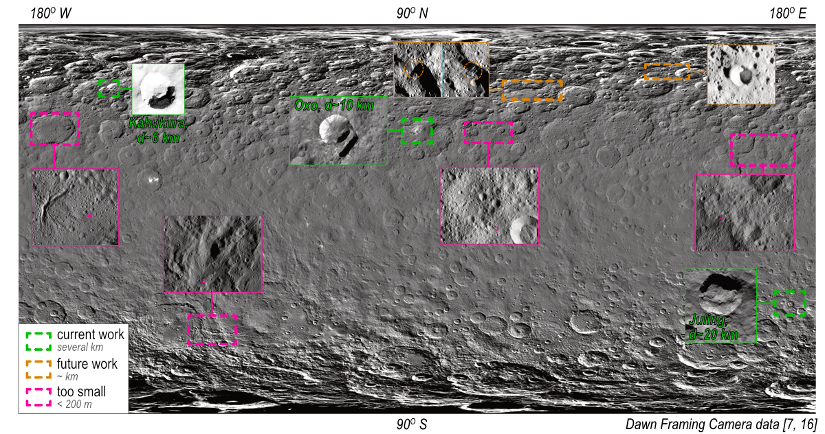
Figure 1. Ice exposures in fresh impact craters, modified from [6].
Here, we investigate the physical form, grain size, purity, and salt content of ice in 3 sufficiently large fresh craters (Figure 1) to constrain ice emplacement mechanisms. We use data from the Dawn Framing Camera (FC; broadband 0.4-1.1 µm filter) [7] to determine the geological setting of ice and the Dawn Visible and Infrared Spectrometer (VIR; 1—5.1 µm) [8] to constrain the physical properties of ice, modeled as intimate (Hapke theory [9]) or areal spectral mixtures with Ceres’ average regolith [10, 11]. We calculate a variety of spectral metrics, e.g., 2 µm band area vs. the 1.1—1.7 µm spectral slope (Figure 2), for both modeled and VIR spectra of ice deposits. These metrics track with ice abundances and grain sizes differently for the mixing modes, which allows us to differentiate between them.
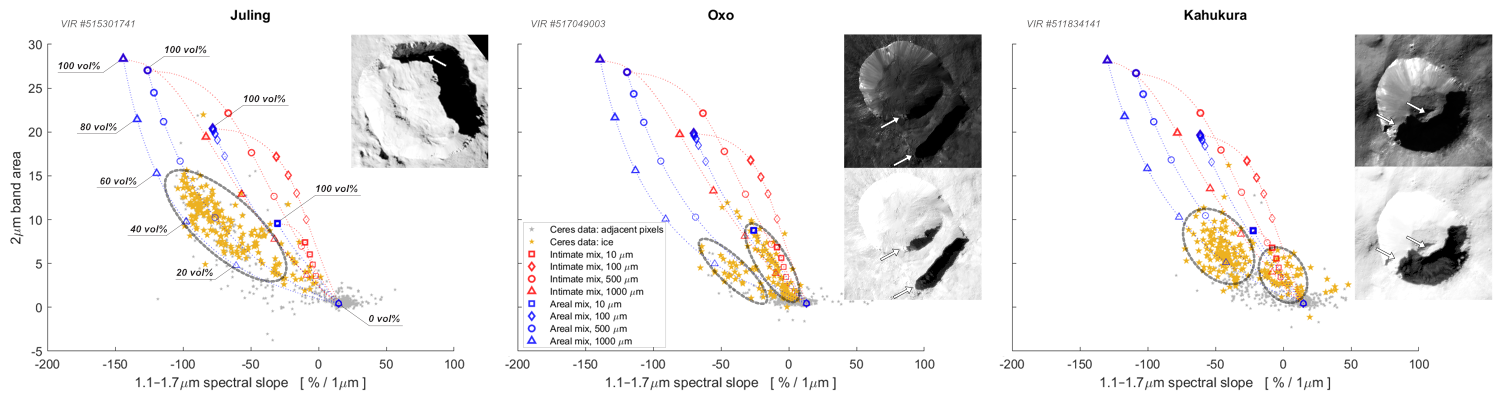
Figure 2. Spectral metrics computed from VIR data and numerical models of ice quantity and grain size for mixtures with local regolith.
Our results show that ice in the studied craters is different (Figure 2), and these variations are intrinsic to the deposits. Juling crater seems to have relatively pure chunks of coarser-grained ice (areal mixes with regolith). Ice in Oxo crater appears to be of two kinds – either well-mixed with regolith (intimate) or in small patches (low abundance areal). Part of the Oxo ice-bearing deposit is sun-illuminated, which suggests a different thermal regime within the same deposit that could explain spectral differences in ice. We see a similar picture in Kahukura crater where ice from the shadowed areas cluster in the parameter space predicted for coarser-grained ice in areal mixtures and ice from illuminated areas is better described by intimate mixes or low abundance areal mixes. This is consistent with thermal processing of ice and ongoing sublimation [e.g., 12–14].
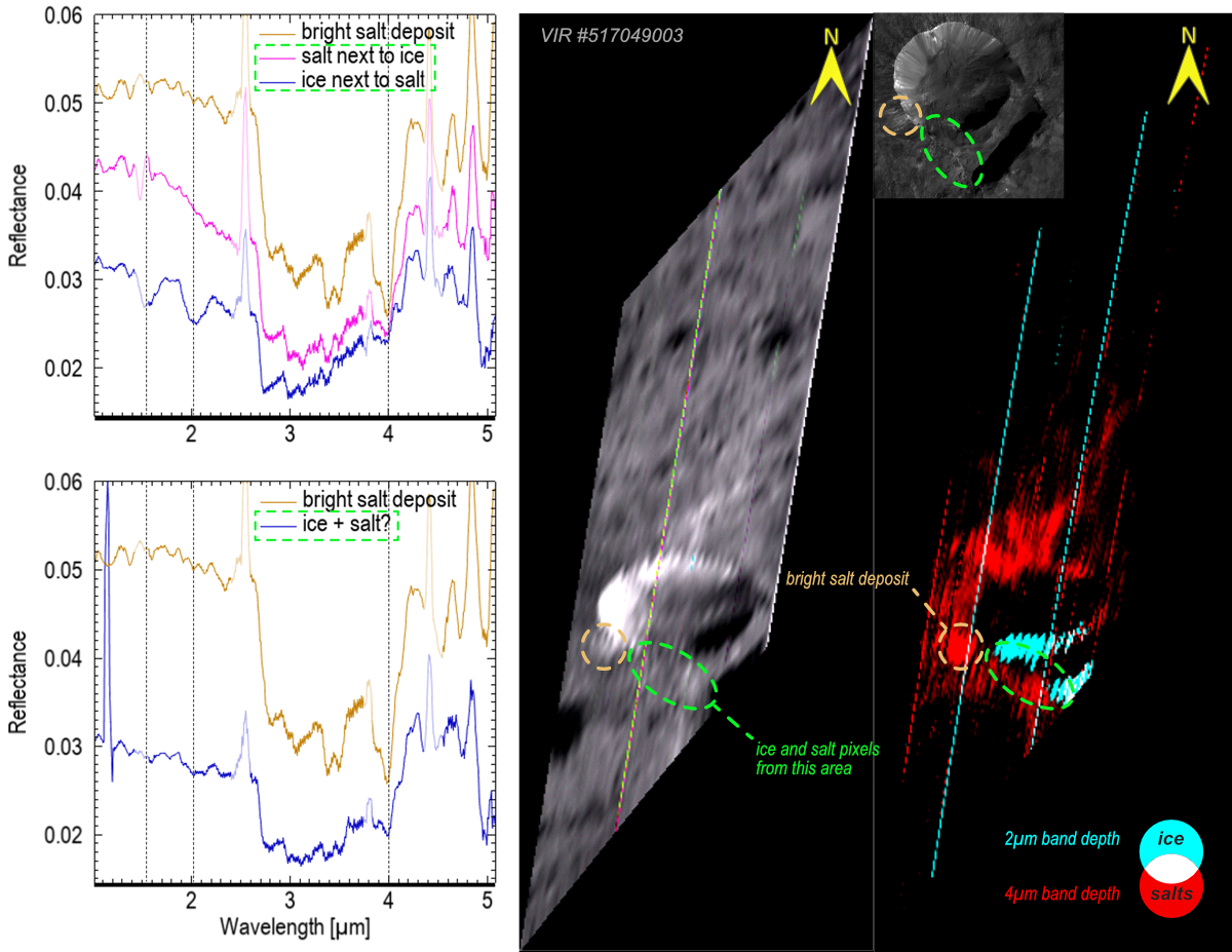
Figure 3. Spectra of mixed ice and salt in Oxo crater.
Finally, we examine whether ice deposits are excavated diapirs of salty ice, whose sublimation is theorized to produce Ceres’ bright sodium carbonate deposits [15]. Spectra of Oxo deposits show suggestive evidence for salty ice, and our ongoing search has revealed no such evidence in the other craters so far. Our spectral modeling of ice+anhydrous sodium carbonate mixtures shows that salt may remain undetected in ice deposits. For intimate mixtures with fine-grained ice, up to 70 vol% of sodium carbonates may be non-detectable.
References: [1] De Sanctis MC & Raponi A in “Vesta and Ceres”, ed. Marchi S et al (2022) ISBN: 97811088563242022; [2] Prettyman TH et al (2017) Science, 355(6320), 55–59; [3] Sizemore HG et al (2018) JGRP, 124(7), 1650–1689; [4] Ermakov AI et al (2017) JGRP, 122(11), 2267–2293; [5] Fu RR et al (2017) EPSL, 476, 153–164; [6] Combe J-Ph et al (2019) Icarus, 318, 22–41; [7] Nathues A et al (2016) Dawn FC2 calibrated Ceres images V1.0, dawn-a-fc2-3-rdr-ceres-images-v1.0, NASA PDS; [8] De Sanctis MC et al (2015) Dawn VIR calibrated Ceres infrared spectra V1.0, dawn-a-vir-3-rdr-ir-ceres-spectra-v1.0, NASA PDS; [9] Hapke B (2012) ISBN: 9781139025683; [10] Kachmar VV et al (2023) LIV LPSC, #1398; [11] Kachmar VV & Ehlmann BL (2024) LV LPSC, #1334; [12] Hayne PO & Aharonson O (2015) JGRP, 120(9), 1567–1584; [13] Nathues A et al (2015) Nature, 528, 237–240; [14] Schorghofer N et al (2024) Planet Sci, 5, 99; [15] Stein N et al (2023) JGRP, 128(7); [16] Roatsch T et al (2016) Dawn FC2 derived Ceres mosaics V1.0, dawn-a-fc2-5-ceresmosaic-v1.0, NASA PDS.
How to cite: Kachmar, V. and Ehlmann, B. L.: Constraining Ceres' exposed ice: grain size, abundance, and is it salty?, Europlanet Science Congress 2024, Berlin, Germany, 8–13 Sep 2024, EPSC2024-677, https://doi.org/10.5194/epsc2024-677, 2024.
- Introduction
Classified as type-V, the basaltic asteroids of the Main Belt (MB), for the most part, are connected to Vesta's dynamic family. However, since the discovery of the V-type asteroid (1459) Magnya in the outer MB, several new asteroids have been found in different regions, including V-types from inner regions not belonging to the Vesta family. These findings suggest that these objects have more than one parental body and can sample multiple differentiated planetesimals, making them an interesting class to study.
Therefore, an interesting method for studying the surface properties of asteroids is through photometric phase curves, which are defined as the study of the scattering of light from a body according to the variation in the solar phase angle. Hence, to determine our phase curves, we use the three-parameter nonlinear model H-G1-G2 developed by Muinonem et al. (2010) and Penttilä et al. (2016), which provides us with the absolute magnitude (H), which is defined as the intrinsic brightness of the object and is related to size, and the curve slope parameters (G1-G2), which are related to surface properties.
- Observations and results
For this study, we selected ten V-types, nine MB asteroids and one NEO, with only one MB belonging to outer MB, (1459) Magnya. To achieve this, data from observations carried out between May 2014 and May 2020, was obtained at the Observatório Astronômico do Sertão de Itaparica (OASI, Brazil), within the framework of the IMPACTON project (Lazzaro et al., 2010).
To investigate the phase curve behavior of V-types, we first analyze the distribution of slope parameters in G(1) vs G(2) phase space for our sample of observed V-types compared to other data, as shown in figure 1. As it can be seen, this is a different result from that obtained by Oszkiewicz et al. (2021) which analyzing V-types in the inner main belt and found a clustering of objects around (4) Vesta. In our sample, some V-types cluster around (4) Vesta, in a region corresponding to objects with moderate to high albedo. Other objects, show a behavior more similar to (1459) Magnya, being located in the region displaying the highest concentration of objects of C-, P- and D-type. Moreover, a few objects, are found completely outside the correlation region. However, as shown by Arcoverde et al. (2023), for MB and NEO small objects, this spread along the correlation trend can be attributed to the small size of the analyzed V-types.
Then, we investigated the behavior of the phase curves in the OE region aiming to characterize their dependence on the object´s albedo. Figure 2 shows the distribution of the amplitude of OE 𝜻 - 1, according to the albedo of each object.
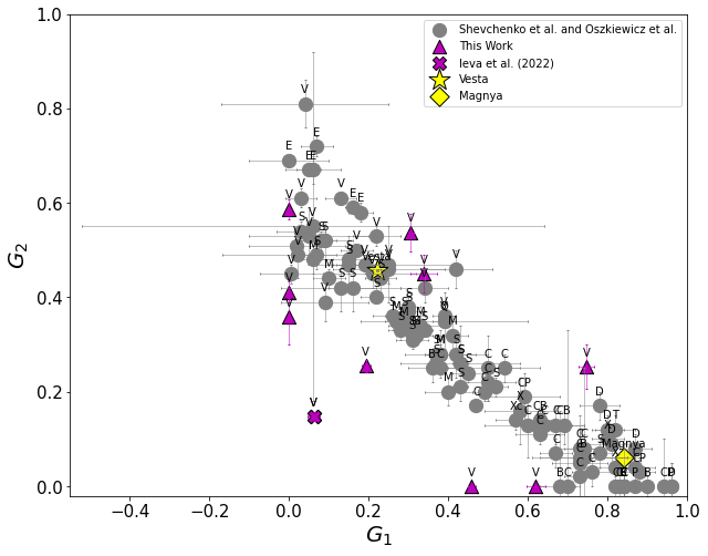
Figure 1: Distribution of slope parameters in phase space G1 vs G2 to observed asteroids. Data from this work and Ieva et al., (2022), indicated by magenta symbols, and Shevchenko et al., (2016) and Oszkiewicz et al., (2021) indicated by gray symbols, highlighting Vesta and Magnya for comparison.
Although all the observed V-type clusters at moderate to high albedo, differently from other taxonomic classes they span a large range of amplitude of the OE. Belskaya et al., (2000) found that the amplitude of the OE varies according to the combined effect of shadow hiding and coherent-backscatter mechanisms, with an increase in amplitude for objects with moderate albedo, and a decrease for those with low and high albedo. In this work, we found the same relationship, but only for large objects. The greatest variation in OE amplitude was found in small objects, diameter of around 10 km including (1459) Magnya (figure 2, right panel), suggesting that the size of the objects has influence on the surface distribution of the regoliths: larger objects are capable of containing finer regolith particles compared to smaller ones, and resulting in the distribution found.
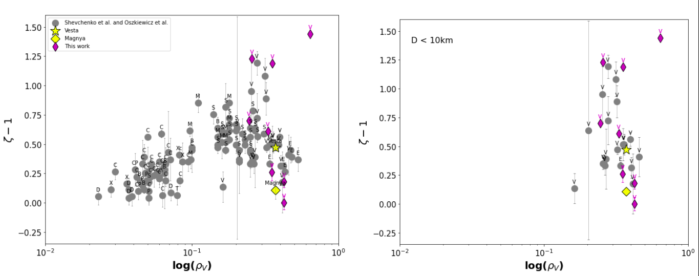
Figure 2: The same distribution of the amplitude of OE 𝜻 - 1, according to the albedo same as Fig. 1. The left panel represents all objects, and the right panel the objects with D < 10km, highlighting Vesta and Magnya for comparison.
Finally, the results obtained here were determined based on high-quality data obtained at the OASI, reinforcing the importance of a dedicated telescope. Nevertheless, more observations of basaltic objects are necessary to better understand the behaviors presented here, especially for the smallest objects and focusing in high-quality phase curves with as much information as possible in the OE region.
Acknowledgements
P.A., E.R., F.M., M.E, W.P. and J.M. would like to thank CNPq, FAPERJ and CAPES for their support through diverse fellowships. Support by CNPq (310964/2020-2) and FAPERJ (E-26/202.841/2017 and E-26/201.001/2021) is acknowledged by D.L. The authors are grateful to the IMPACTON team, in special to R. Souza, A. Santiago and J. Silva for the technical support.
References
Arcoverde P., et al., 2023, MNRAS, 523, 739
Belskaya I. N., Shevchenko V. G., 2000, Icarus, 147, 94.
Ieva S., et al., 2022, MNRAS, 5313, 3104.
Lazzaro D., 2010, Boletin de la Asociacion Argentina de Astronomia La Plata Argentina, 53- 315.
Muinonen K., Belskaya I. N., Cellino A., Delbò M., Levasseur-Regourd A.-C., Penttilä A., Tedesco E. F., 2010, Icarus, 209, 542.
Oszkiewicz D., et al., 2021, Icarus, 357, 114158
Penttilä A., Shevchenko V. G., Wilkman O., Muinonen K., 2016, Planetary and Space Science, 123, 117.
How to cite: Arcoverde, P., Pereira, W., Rondón, E., Monteiro, F., Evangelista-Santana, M., Michimani, J., Medeiros, H., Silva-Cabrera, J., Rodrigues, T., and Lazzaro, D.: Study of basaltic asteroids through their phase curves, Europlanet Science Congress 2024, Berlin, Germany, 8–13 Sep 2024, EPSC2024-999, https://doi.org/10.5194/epsc2024-999, 2024.
Please decide on your access
Please use the buttons below to download the supplementary material or to visit the external website where the presentation is linked. Regarding the external link, please note that Copernicus Meetings cannot accept any liability for the content and the website you will visit.
Forward to presentation link
You are going to open an external link to the presentation as indicated by the authors. Copernicus Meetings cannot accept any liability for the content and the website you will visit.
We are sorry, but presentations are only available for users who registered for the conference. Thank you.
INTRODUCTION
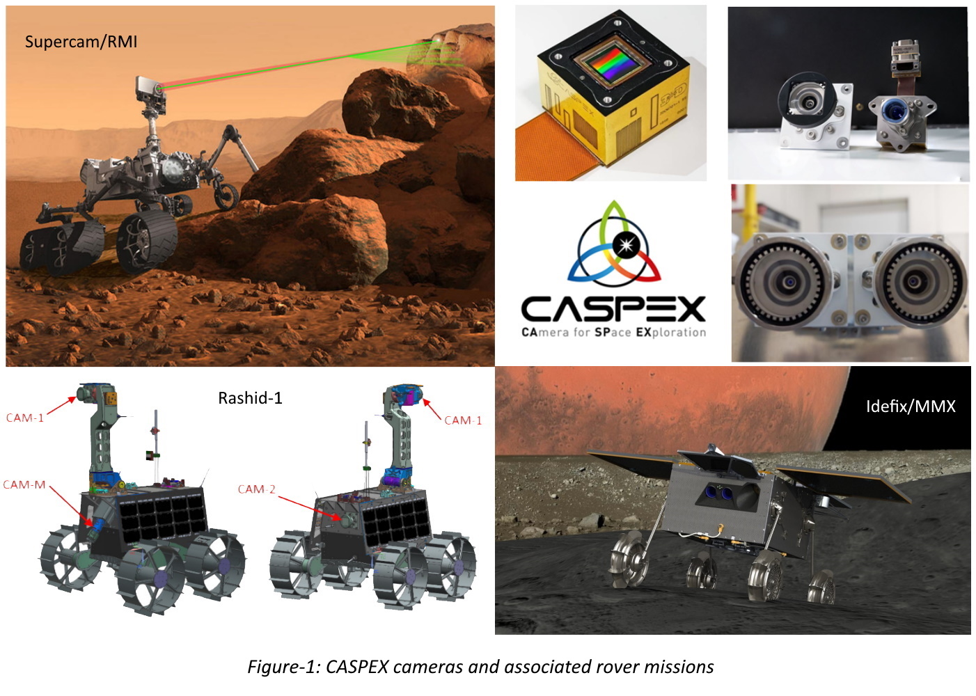
To meet the needs of space exploration missions, CNES and its industrial partner 3D+ have developed a series of dedicated cameras called CASPEX[1] (Figure-1). These cameras consist of two parts:
- A detector unit with different numbers of pixels and spectral ranges, as well as filters deposited on it (color, polarization),
- An optical unit mounted on the detector, with different functional points, such as wide-angle cameras for navigation, or tilted proximity cameras to study the composition of the ground under millimeter resolution.
Such cameras are used on Supercam/RMI aboard Perseverance[2] and will be used on the MBRSC Rashid[3][5] rovers and on the CNES/DLR Idefix[4] rover aboard the JAXA MMX mission.
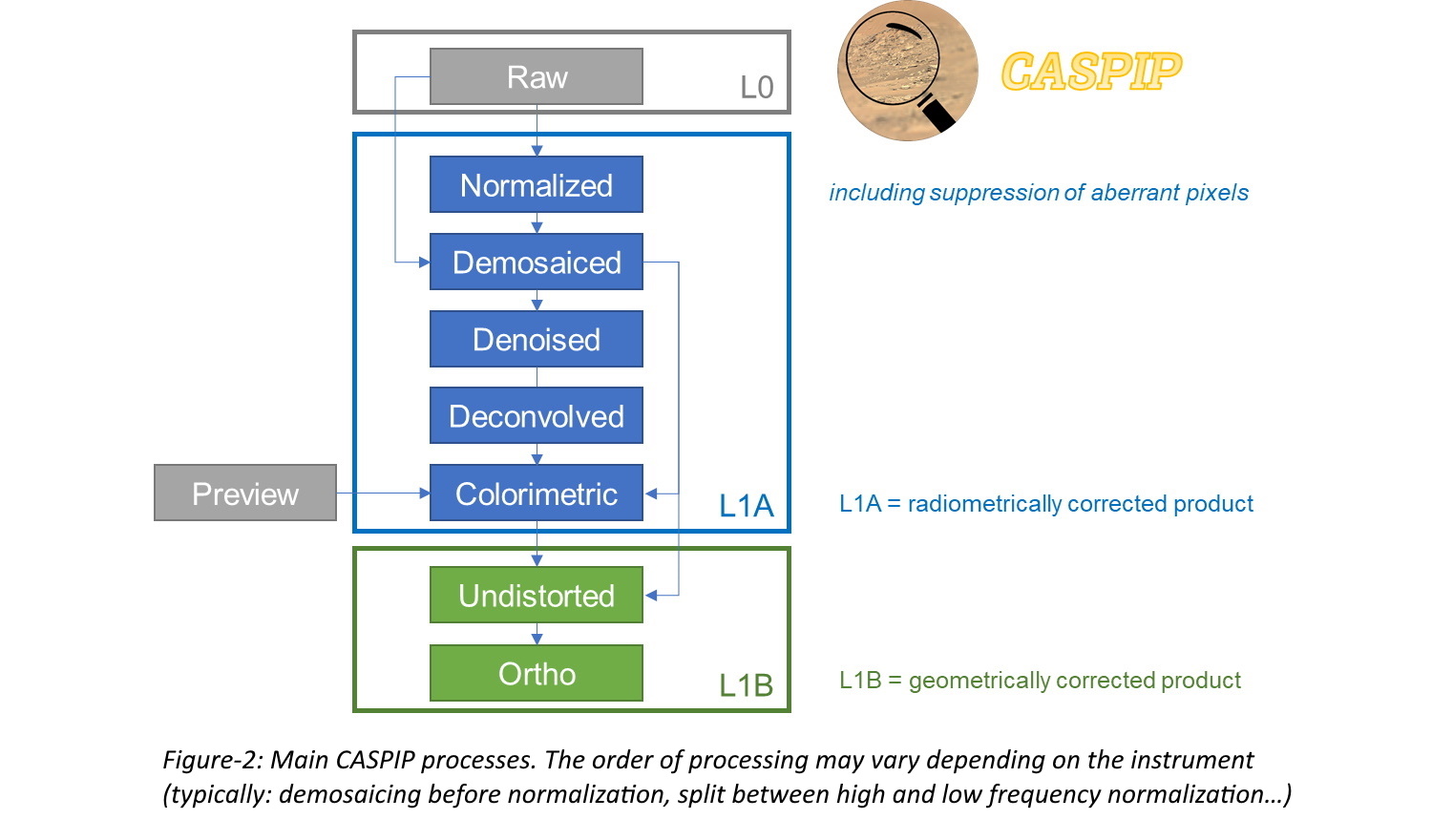
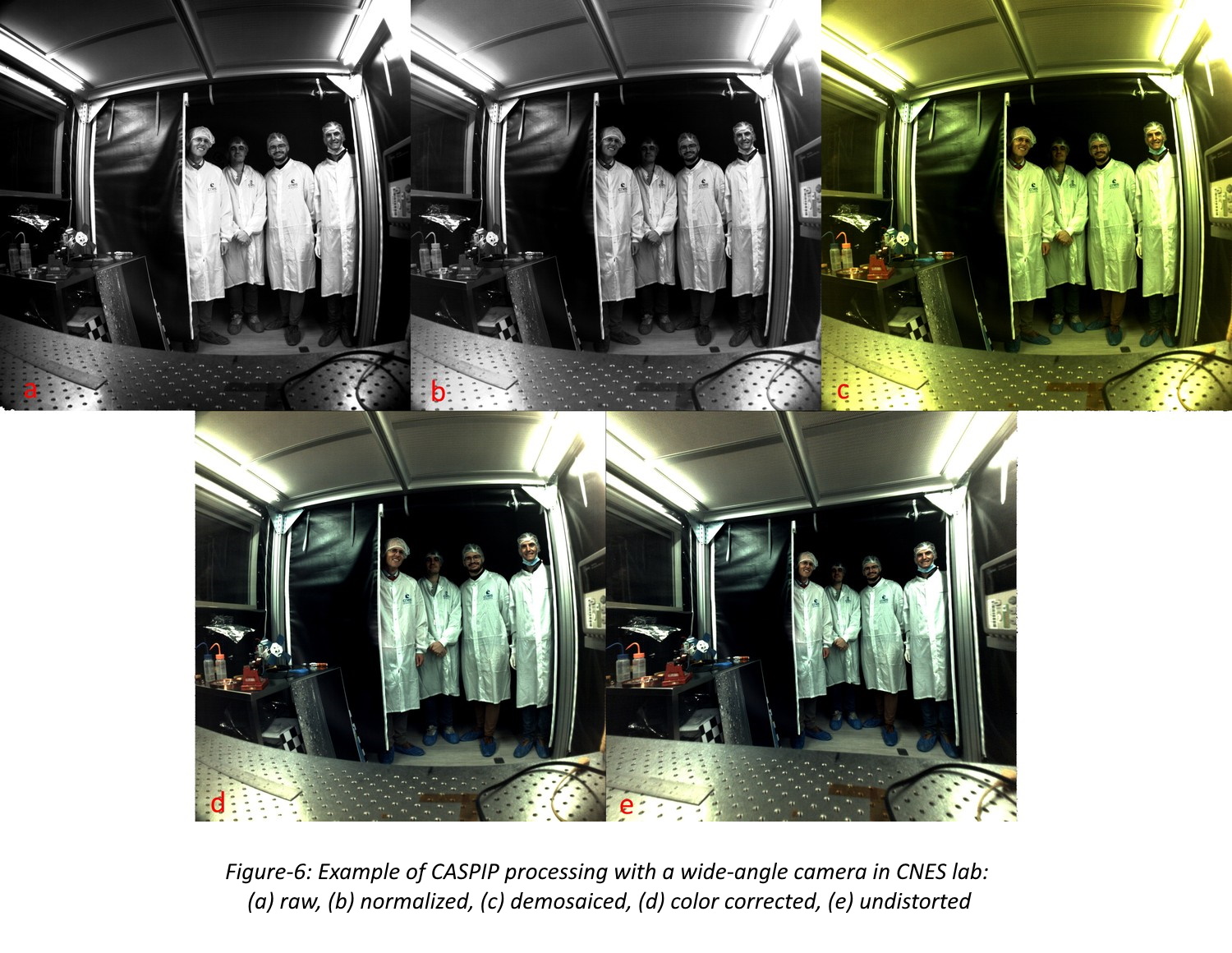
CASPEX Image Processing (CASPIP) is a tool used for the first-level correction processing of the raw images captured by these cameras (Figure-2).
CASPIP SOFTWARE DESCRIPTION
CASPIP is an “easy-to-use” Python library developed at CNES and distributed on https://www.connectbycnes.fr/en/caspip. It works on Linux and Windows. The configuration parameters are grouped in a “camera” object, so that it is possible to define several cameras in one run. The calling interface is step-by-step and as simple as follows:
processed_image = caspip_function(my_camera, image_to_process, (optional parameters))
In addition to the main functions shown in Figure-2, some tools are added, such as direct and inverse localization functions and distance measurements, as well as a GUI visualization tool.
CASPIP can be used also for enhanced image processing[5], such as 3D reconstruction.
MAIN FUNCTIONS
Radiometric processing
CASPEX detectors have a PRNU (Photon Response Non Uniformity) of less than 1.35%[1] and very few defective pixels[1]. Despite such low levels, CASPIP can use ground data to correct – if needed – PRNU effects, as well as interpolate missing pixels in the image.
The wide-angle cameras induce a strong low-frequency vignetting effect (Figure-6, a→b), which can also be observed on various cameras, such as Supercam/RMI (Figure-3, a→b). The vignetting is corrected by dividing by a flat-field reference image.
Typical color filter arrays provide a sparse representation of the spectral bands using a Bayer pattern, alternating red, blue and green pixels. It is important to perform a ‘demosaicing’ step, to ensure that the final RGB image has the same resolution as the detectors. Several methods can be used for demosaicing, with the most common being based on interpolation. CASPIP implements the Hamilton-Adams[7] (Figure-6, b→c) and Malvar[8] algorithms by default, although several other techniques can be implemented instead, such as Bayesian approaches[6], but with increased computational complexity.
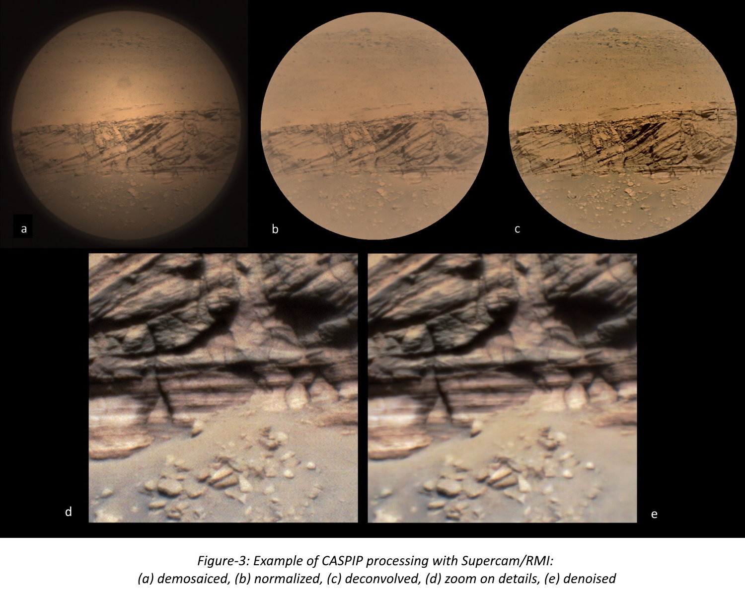
Knowing the Modulation Transfer Function (MTF) of the instrument, preferably by in-situ measurements, it is possible to add a deconvolution step to reverse instrument blurring and sharpen the final images. Depending on the camera and the optical design, this step may be necessary (Supercam/RMI – Figure-3, b→c – in this case, the image is oversampled regarding the optical resolution).
Before deconvolving, it is necessary to reduce the noise, which should be increased by the processing: CASPIP implements a NL-Bayes denoising technique[6] (Figure-3, d→e).
Finally, a colorimetric correction has to be applied for the image to be expressed in a standard camera-independent color space. This is done by applying a correction matrix calculated following the ISO/CIE 11664-3 standard.
Geometric corrections
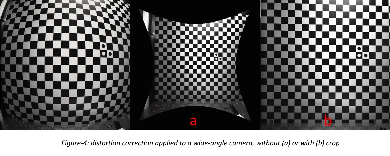
Wide-angle cameras cause an important distortion effect that can be corrected by applying a polynomial[5] to the (x,y) coordinates (Figure-6, d→e). This processing causes a deformation of the image, which is no longer on a regular square grid: we can either crop it or keep the whole image (Figure-4), depending on our needs. The resulting image is nominally regularly sampled with a pixel size in the center of the field still equal to the original resolution.
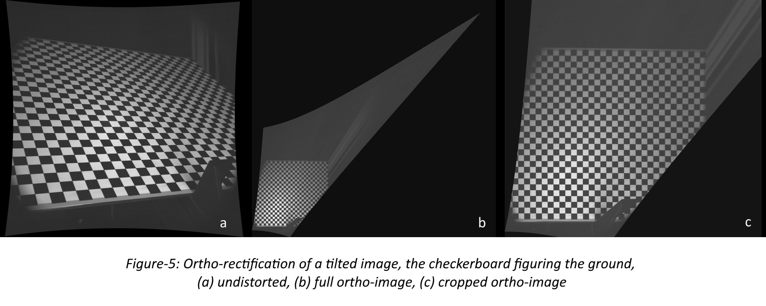
Observing the microscopic structure of the ground near the rover requires pointing the camera in a tilted direction, which results in a distorted image because the observed plane is not perpendicular to the pointing direction. This is the case for CAM-M on Rashid-1 and for the MMX wheel cameras, which observe the interaction between the wheels and the regolith. CASPIP allows the calculation of "ortho-images" using the value of the tilt angles (Figure-5). If the ground surface is not flat, residual distortion effects are still expected on the result.
FURTHER DEVELOPMENTS
Since proximity cameras have a very small depth of field, an object (rock) or a hole will cause defocus to increase in the field of view. We will then develop a function to make the deconvolution variable across the detector field of view.
Future CASPEX cameras will also include complex filter arrays[9] with typically 8 or 25 spectral bands, which will require a specific "demosaicing" function. We are working on new solutions that will be implemented in CASPIP. Such cameras and processing will allow both a spectral capability and a good spatial resolution without moving parts such as filter wheels.
Other developments can be considered in the framework of the collaboration with CNES for new space exploration missions.
REFERENCES
[1] Virmontois, C. et al, CASPEX: Camera for space exploration, in preparation (2024)
[2] Wiens, R.C., Maurice, S. et al, Space Sci. Rev. 217, 4 (2021),
https://doi.org/10.1007/s11214-020-00777-5
[3] Els, S.G., Almarzooqi, H. et al, Space Sci. Rev, under submission (2024)
[4] Michel, P. et al, Earth, Planets and Space 74(1), 2 (2022),
https://doi.org/10.1186/s40623-021-01464-7
[5] Théret, N. et al, Space Sci. Rev, under submission (2024)
[6] M. Lebrun et al, IPOL, vol.3, pp.1-42 (2013), http://dx.doi.org/10.1137/120874989
[7] Hamilton J.F.Jr., Adams J.E.Jr., Patent US5629734A (1996),
https://patents.google.com/patent/US5629734A/en
[8] Malvar, H.S. et al, International Conference on Acoustics, Speech, and Signal Processing,
pp.iii-485 (2004), https://doi.org/10.1109/ICASSP.2004.1326587
[9] Cucchetti, E. et al, Color and Imaging Conf., pp205-212 (2022),
https://doi.org/10.2352/CIC.2022.30.1.36
How to cite: Théret, N., Douaglin, Q., Cucchetti, E., Robert, E., Lucas, S., Lalucaa, V., and Virmontois, C.: CASPEX Image Processing: a tool for space exploration, Europlanet Science Congress 2024, Berlin, Germany, 8–13 Sep 2024, EPSC2024-15, https://doi.org/10.5194/epsc2024-15, 2024.
Introduction: The Context Camera (CTX) has so far delivered more than 145,000 images [1]. The images are one of the most popular datasets for planetary geologists, providing extensive coverage, excellent radiometric resolution, and a unique resource for interpreting surface features. The Integrated Software for Imagers and Spectrometers (ISIS) is a software to support the ingestion, processing and analysis of planetary image data [2] and is the standard processing framework for CTX. Since the beginning of its mission, calibrated images from CTX have shown a subtle darkening effect from the centre of the image towards the edges. Due to its typical shape when plotted as a profile, this effect has been called the "frown" effect (see Figure 1).
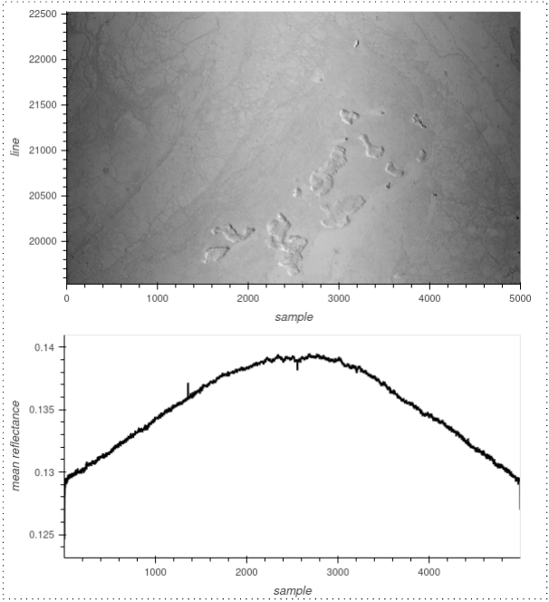
Figure 1: Subset of CTX image G09_021566_1800 after nominal ISIS calibration together with a plot of the reflectance values averaged over all lines [3].
Some authors assume a varying darkening effect over the mission time, and workarounds to correct for this have been described [4,5]. Here we present an updated flat-field calibration for ISIS that removes the edge darkening effect. We ensure that it does not introduce any artefacts and perform quantitative validation of calibrated images to show the validity of the improvements.
Methods: The overall shape of the CTX flat-field is a curve, where the difference between the centre and the edges of the detector represents a quantifiable amount of darkening caused by lens vignetting. To quantify the amount of this edge darkening correction by a flat-field, we use the concept of the frown factor. Similar to the quantification of the band depth feature in spectral analysis, the amount of darkening correction by a flat-field can be expressed as the ratio of the mean values of the central area of the flat field to the mean values of its edges (see Figure 2).

Figure 2: Elements for the composition of the frown factor of a flat-field [3].
Before building a flat-field from a pool of input images, we correct the input data from bias and dark-current effects without any initial flat-field correction. As the ISIS ctxcal command combines these two corrections, we turn off the flat-field correction in ctxcal by providing a custom flat-field file where all values are set to one. We use the resulting pre-processed bias/dark-current corrected files for calculating the new flat-field.
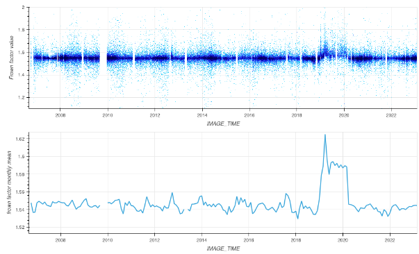
Figure 3: Top: Scatter plot of the frown factor over time. Bottom: mean monthly frown factor over time [3].
Results: Figure 3 shows the temporal evolution and distribution of the frown factor, i.e. the amount of darkening towards the detector edges. We exclude images exhibiting overexposure or the ones with negative reflectance values after calibration. The frown factor remains relatively consistent around its mean of 1.55 until the end of 2018, followed by a subsequent rise until early 2020. Throughout this interval, the average frown factor for all images rises to approximately 1.6, and throughout 2020, it reverts to the value observed before the mentioned change.
Investigating the distribution of the frown factor excluding images from the problematic year 2019, we observe a skewed data distribution (Figure 4 right). As the frown factor outside the irregular time interval from 2019 until early 2020 appears very stable, we can safely assume that the edge-darkening effect is stable over time. The deviation from its mean during the period in question is not representative, as the central limit theorem is not fulfilled, which we observe in its non-symmetrical distribution.

Figure 4: Kernel density plot of the frown factor of all images except the ones from the year 2019 (left) compared with the ones from year 2019 (right) [3].
Evaluation: One of the main advantages of the improved calibration is better in-image stability for image mosaicking, which leads to homogeneous mosaics. An example of this is provided in Figure 5. The seams between adjacent images are strongly visible in the "before" mosaic (case a), processed with the nominal flat-field in ISIS. Using our new flat-field calibration file, most seams are no longer visible (case b).
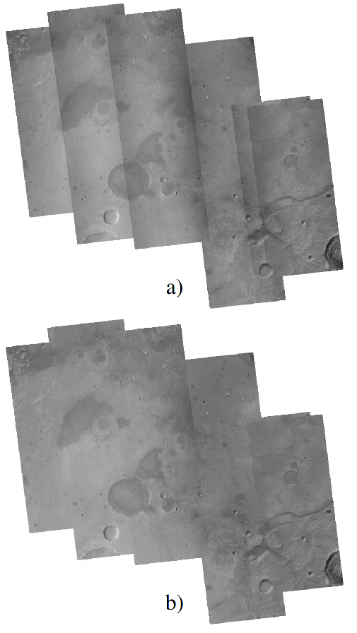
Figure 5: Example CTX mosaic of the Oxia Planum region. Images were chosen from Martian Year 33. a) calibrated with the nominal ISIS internal flat-field calibration – b) calibrated with the new global flat-field calibration [3].
For a quantitative evaluation, we randomly chose 10.000 images over the full timespan and calibrated them with our new flat-field file when using ctxcal. The arithmetic mean of the frown factor of these images is then 1.00, proving a very good result and confirming the frown factor as a good quantification. We randomly reduced the subset to 1.000 images and performed a systematic visual inspection for qualitative evaluation. We could not find any signs of a remaining edge-darkening effect during the visual investigation. The residual edge-darkening effect is 1.079, calculated as the arithmetic mean over the individual factors of all images from the validation dataset calibrated with the previous flat-field file. This means, a surface recflectance measurement taken at the edge of a CTX image appears 8% darker than in the center, when calibrated with the previously available flat-field file.
The new flat-field calibration file is available from this data repository: http://dx.doi.org/10.17169/refubium-41645. It has also been provided to the ISIS development team in order to publish it in their default data directory, beginning with ISIS version 9.0.
Acknowledgements: This work is supported by the German Space Agency (DLR Bonn), grant 50 OO 2204, on behalf of the German Federal Ministry for Economic Affairs and Energy.
References: [1] M. C. Malin et al., JGR Planets (2007). [2] Jason Laura et al., 2023, DOI: 10.5281/zenodo.2563341. [3] Walter, et al., ESS 11 (2024), DOI: 10.1029/2023EA003491. [4] J. L. Dickson et al., LPSC 49 (2018), #2480. [5] Stuart J. Robbins et al., ESS 10 (2020).
How to cite: Walter, S., Aye, M., Jaumann, R., and Postberg, F.: Mars Reconnaissance Orbiter Context Camera updated in-flight calibration, Europlanet Science Congress 2024, Berlin, Germany, 8–13 Sep 2024, EPSC2024-77, https://doi.org/10.5194/epsc2024-77, 2024.
We present recent advances in our Asteroid Imaging Simulator (AIS) toolset [1]. The purpose of the tool is to support the design and operating planning of imaging instruments in space missions. In particular, we aim to support the hyperspectral camera units from VTT Finland in ESA Hera mission (ASPECT camera, Milani CubeSat) and in Comet Interceptor mission (part of MIRMIS instrument).
The tool consists of two main parts. The part generating simulated imagery is based on Blender ray-tracing software [2], and the part converting the images into image data with physical units and simulated instrument noises is written in Python. The Blender part utilizes the internal Python interpreter on Blender and all the tools from the Blender GUI. Our Python module and Blender file enable using shape models as targets, e.g., we have Benny, Ryugu, Itokawa, Didymos-Dimorphos, and 67P/Churyumov–Gerasimenko as possible targets. Additionally, we concentrate on providing typical photometric models for the target surfaces including Lommel-Seeliger, ROLO, McEwen, and Lambert photometric functions that are implemented using Blenders’ shaders. The coordinate and attitude information from SPICE kernels is integrated into our Blender package, as well as scripts for creating circular or elliptical orbits around the target or fly-by scenarios.
The most recent activity is in the coma model to be used with the Comet Interceptor mission. As we aim to simulate and help camera operations, the actual structure of the coma or jet structure etc. is not of main interest to us, whereas the scattering properties of gas and dust in the coma, given some simple model of their density around the nucleus, is. We will present the first evaluation of the gas and dust coma effects on the scattering in the simulated images of a comet nucleus and surrounding environment. We will concentrate on the target scenarios of Comet Interceptor.
Our post-processing Python package handles the conversion of unitless images from Blender into simulated data stream from an imaging unit with physical units and noises. We will first convert the image color (grayscale) space into spectral radiance in W/m2/nm/sr with the knowledge of target albedo, reflectance spectra, and its distance to Sun. Second, knowing the camera and detector specifications, we can convert all the way into charge counts on the CCD pixel with given integration time. Finally, the detector noise profile allows to compute the expected signal-to-noise ratio of the observations, and to simulate the output data stream with noises. This helps in designing integration times and verifying, e.g., reliable detection of features in the retrieved spectrum.
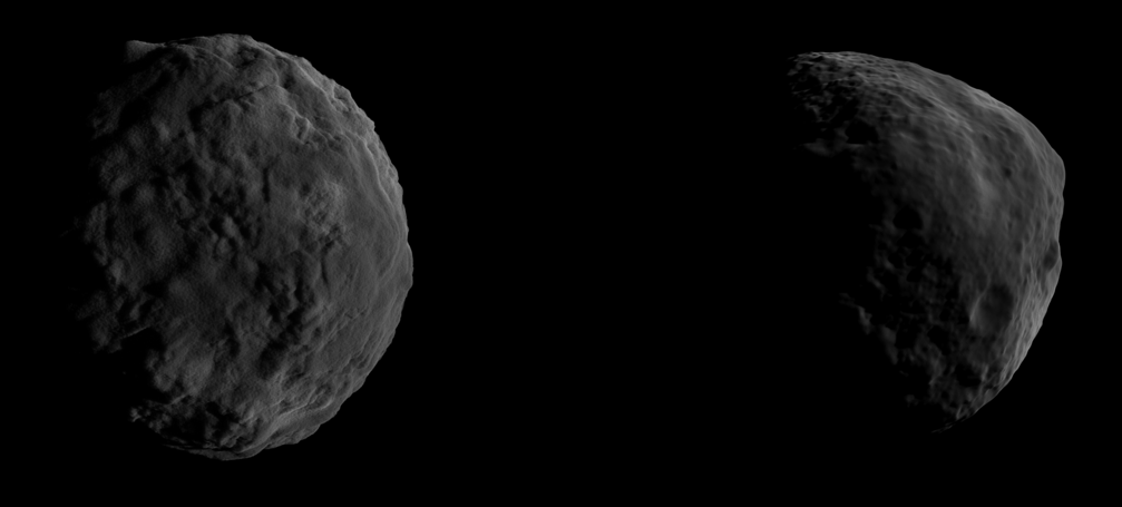
Figure 1: Example of generated images using the shape model of Bennu in two camera positions.
[1] Git project for the Asteroid Imaging Simulator, https://bitbucket.org/planetarysystemresearch/asteroid-image-simulator/
[2] Blender software, https://www.blender.org
How to cite: Penttilä, A., Kolehmainen, M., Halla-aho, N., Jääskeläinen, J., Palos, M. F., Näsilä, A., Cole, R., and Kohout, T.: Imaging instrument simulations for ESA Hera and Comet Interceptor missions, Europlanet Science Congress 2024, Berlin, Germany, 8–13 Sep 2024, EPSC2024-345, https://doi.org/10.5194/epsc2024-345, 2024.
Introduction
Major rock-forming minerals such as pyroxenes are very common in the solar system and show characteristic absorption bands due to Fe2+ in the VIS and NIR [e.g., 1, 2]. The Fe-free endmember enstatite is also probably a common mineral on planetary surfaces such as E-type asteroids and Mercury [3] and a major constituent of meteorites such as aubrites [4] and enstatite chondrites [5]. Reflectance spectra of these meteorites as well as of enstatite-rich or generally Fe-poor asteroids like E-type asteroids and Mercury are often featureless in the VIS and NIR, lacking the absorption features associated with iron incorporated into the crystal structure of silicates, while Fe-bearing orthopyroxenes show diagnostic absorption bands at ~1 µm and ~2 µm [1,2].
For a better understanding of these Fe-poor bodies, the availability of laboratory spectra of Fe-free silicates as analog materials is crucial, but terrestrial samples of enstatite usually contain several mol% of FeO, with pure enstatite being extremely rare. In order to make larger amounts of pure enstatite readily available, we have synthesized nearly FeO-free enstatite [6].
We present 0.3-16 µm reflectance spectra of synthetic enstatite (Mg2Si2O6), synthetic oldhamite (CaS), and of their mixtures [7] for comparison with spectra of E[II]-type asteroids, investigate the spectral behavior of the mixtures with respect to their oldhamite content, and discuss the implications for surface composition analysis of Mercury.
Selection of Samples
All reflectance spectra were collected using a Bruker Vertex 80v FTIR spectrometer at the Planetary Spectroscopy Laboratory of the Institute of Planetary Research at DLR, Berlin [8]. The synthesis of the enstatite sample with the composition En99.6Fs0.0Wo0.4 has been described in detail by [6]. The oldhamite sample was purchased from abcr GmbH (99.95 %, metal basis, CAS #20548-54-3). The average grain size of the enstatite and oldhamite samples are 26 µm and 12 µm respectively [6,7]. Mixtures containing 1, 3, 5, 10, 20, 30, 40, 50, 60, 70, 80, and 90 vol% oldhamite were prepared.
Results
Figure 1 shows the reflectance spectra from 0.3 to 1 µm. The enstatite spectrum shows several weaker absorption bands between 0.4 µm and 1 µm which are due to Fe3+ and possibly Ti and shows a steep red slope in the UV. The spectral slopes in the VIS and NIR are nearly neutral with only a slightly reddish slope in the VIS. The spectrum of synthetic oldhamite shows an absorption band at 0.41 μm with a relative depth of 11.4 %. This band is visible in the spectra of all mixtures, even in the spectrum of the mixture containing only 1 vol% oldhamite. In the MIR, the spectra with ≤10 vol% oldhamite are very similar to the spectrum of the pure enstatite and are generally dominated by the Christiansen feature (CF) and the Reststrahlen bands (RB). The pure oldhamite is significantly brighter than the enstatite spectrum in the MIR and shows several broad and overlapping absorption features (figure 2). Changes in the band depth and reflectance, both in the VIS and MIR, do not occur as a single trend, but follow two distinct trends. One for mixtures with ≤10 vol% of oldhamite, where changes rapidly occur, and another trend for mixtures with ≥20 vol% of oldhamite, where changes occur more slowly.
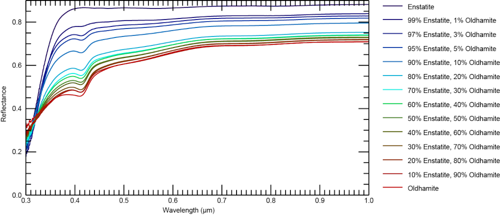
Figure 1. Reflectance spectra of synthetic enstatite, oldhamite, and their mixtures from 0.3 to 1 µm. Compositions are given in vol%.
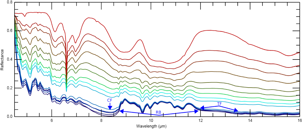
Figure 2. MIR reflectance spectra from 7 to 16 µm of synthetic enstatite, oldhamite, and their mixtures. For legend see figure 1.
Discussion
Based on XRS data, sulfur contents up to 4 wt% have been reported in surface materials of Mercury [9], and sulfide decomposition has been linked to the formation of hollows on Mercury [10], geological features unique to the surface of Mercury. Oldhamite was proposed as the major lithophile sulfide on the surface of Mercury [11]. Therefore, understanding the spectral behavior of oldhamite in mixtures with FeO-poor silicates, such as enstatite, is crucial for the interpretation of spectral data from Mercury. Figure 3 shows a comparison between a Mercury spectrum [12,13], the aubrite Peña Blanca Spring (PBS) [6], and selected laboratory spectra from this study. The positions of the CF and RB in these spectra are in good agreement. The RBs are less pronounced in the enstatite and PBS spectra than in the Mercury spectrum. The oldhamite spectrum has a local maximum at ~9.5 µm, which could contribute to the higher reflectance in this wavelength range compared to the enstatite and PBS.
The influence of space weathering on FeO-poor surfaces such as Mercury is still poorly understood. Factors such as thermal degradation or the influence of grain size changes have been discussed. However, many important influencing factors are still unknown [7]. Spectral investigations of the samples at Mercury-relevant surface temperatures can improve our understanding of these processes. At the same time, such studies would improve the comparability of Mercury spectra with those of the analogous materials measured here at room temperature.
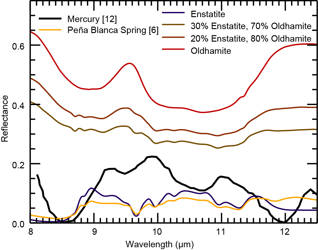
Figure 3. Comparison between a Mercury spectrum [12,13], Peña Blanca Spring spectrum [6], and selected laboratory spectra from this study. The Mercury spectrum was obtained by [12] and converted to reflectance using Kirchhoff’s law and baseline corrected by [13]. Compositions are given in vol%.
References
[1] Burns (1993) Mineralogical Applications of Crystal Field Theory, 2nd ed. [2] Klima et al. (2007) Met. Planet. Sci., 42, 235-253. [3] Izenberg et al. (2014) Icarus, 228, 364-374. [4] Keil (2010) Chem. Erde, 70, 295-317. [5] Mason (1968) Lithos, 1, 1-11. [6] Markus et al. (2018) Planet. Space Sci., 159, 43-55. [7] Markus et al. (2024) Planet. Space Sci., 244, 105887. [8] Maturilli and Helbert (2019) LPSC, 1846. [9] Nittler et al. (2011) Science, 333, 1847-1850. [10] Blewett et al. (2013) JGR Planets, 118, 1013-1032. [11] Vaughan et al. (2013) LPSC, 1719. [12] Sprague et al. (2000) Icarus, 147, 421-432. [13] Morlok et al. (2020) Met. Planet. Sci., 55, 2080-2096.
How to cite: Markus, K., Arnold, G., Moroz, L., Henckel, D., and Hiesinger, H.: Laboratory reflectance spectra of enstatite and oldhamite mixtures for comparison with E-type asteroids and implications for Mercury’s surface composition analysis, Europlanet Science Congress 2024, Berlin, Germany, 8–13 Sep 2024, EPSC2024-446, https://doi.org/10.5194/epsc2024-446, 2024.
Introduction:
The JAXA/Martian Moon eXploration (MMX) mission will be launched to the Martian system in 2026 with the objective of deciphering the origins of Phobos and Deimos [1]. One of the instruments onboard the MMX spacecraft will be MIRS, an imaging-infrared spectrometer covering a wavelength range from 0.9 µm to 3.6 µm [2]. In this work, we will present simulations of MIRS imaging of Phobos realized to prepare the future science exploitation of MIRS data and assess instrument performances. These simulations will also be useful during the operations of MIRS to anticipate the operations such as the Deimos flybys and Phobos landing.
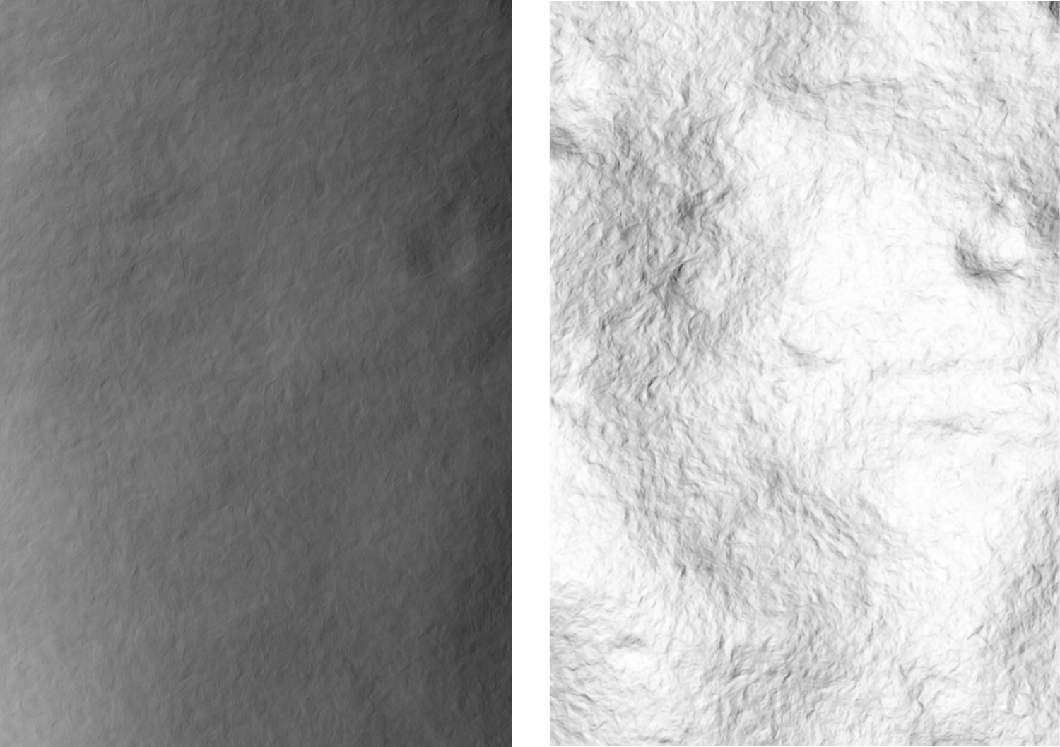
Figure 1: Example of surface reflectance at 1 µm (left) and temperature at 3 µm (right) landscapes obtained with OASIS simulation.
Method:
The generation of a spectral MIRS image is obtained with the use of a suit of three simulators. The observation mission scenarios are initially derived through AURORA [3], which provides all necessary orbital and instrument information, including the spacecraft position, pointing, etc. The second simulator, OASIS [4], is dedicated to the generation of all the geometric information (incidence, emission, phase, etc.) for each pixel/facet of the Phobos surface. AURORA provides the observation geometries fed into OASIS. The tool considers topographic variation on the surface through the use of the Phobos shape model. From the obtained illumination angles, a Hapke model is used to compute the bidirectional reflectance. The thermal component of the spectra is accounted for, through the use of a Standard Thermal Model. The current model does not account for multiple scattering and Mars reflected light on Phobos and Deimos.
To avoid extremely long computational time, the geometric calculations are only performed at a single wavelength. The spatial and spectral terms of the solar and thermal irradiance are decoupled to allow extrapolation of a spectrum from the simulated landscape.
After generating the reflectance and temperature maps (Fig. 1), the MIRAGES simulator [5] is run to model the MIRS instrument response, including light propagation through the mirrors, grating, and other optical elements, as well as accounting for the radiometric efficiency of these components, and introducing a geometric distortion. This allows to obtain 2D MIRS raw images. In the final stage, the images are processed further using a portion of the MIRS pipeline to obtain corrected and calibrated images. This includes distortion correction, ADU to I/F conversion, and spectral registration procedures. A thermal correction is subsequently applied to remove the contribution of the thermal tail.
Results:
The MIRS images were simulated for two scheduled observations of Phobos, designated as QSO-H (quasi-stationary orbit at high altitude) and QSO-M (quasi-stationary orbit at medium altitude). A typical rendered image for a QSO-H orbit is presented in Fig. 2.
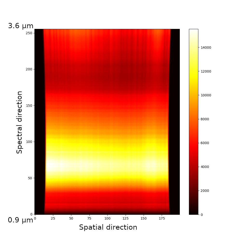
Figure 2: Example of a typical MIRS image for QSO-H orbit, obtained after the three simulators.
In addition to the interest of having the capacity to simulate relatively rapidly MIRS images, we also investigated the detectability of several components of interest for the Phobos’ surface. In particular, we assessed the detectability of small patches of hydrated minerals and organics at the surface of Phobos by MIRS. For this purpose, we used as input, the experimental spectra obtained in our previous works for detectability studies in a Phobos regolith simulant [6,7]. We defined patches of different sizes from a diameter of 3.5 km to 12.9 m at the surface of Phobos. We found that the homogeneous patches are visible in the QSO-H orbit for a diameter of approximately 40 m but not visible when the diameter is reduced to ~13 m. This is in agreement with the expected spatial resolution in the QSO-H orbit which was estimated to be between 31 and 66 m/px. An example of a MIRS observation sequence is presented in Fig. 3. Whereas MIRS images 1 and 2 of the figure correspond to a “classic” area on Phobos, image 3 clearly shows a bright line at the center of the images. This bright line corresponds to MIRS scanning over a small patch of phyllosilicate in our simulated Phobos surface model.
From these 2D images, it is possible to extract the 1D spectrum of both organic and classic Phobos regions. Typical obtained spectra are presented in Fig. 3 (bottom-left corner panel). The contrast between the two regions is evident when looking at the 2.7 µm region, where an absorption band is visible in the case of the phyllosilicates-rich patch compared to the classic Phobos surface.
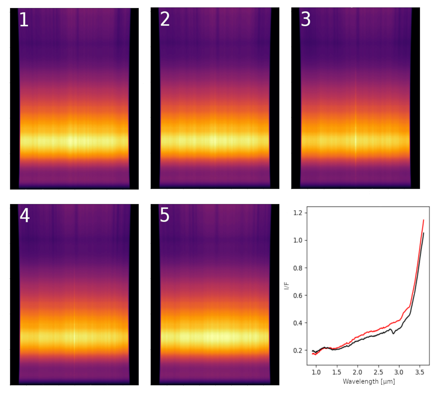
Figure 3: Example of 5 images of a MIRS observation sequence on a landscape obtained by OASIS. The passage on the hydrated mineral patch can be visually seen as a bright line through the spectral direction in the center of images 3 and 4. Bottom left corner: Example of two 1D spectra extracted for a MIRS image (panel 3), before thermal tail removal. The black solid line corresponds to the phyllosilicate patch MIRS rendered spectrum, and the red solid line corresponds to the ‘classic’ Phobos surface MIRS spectrum. The 2.7 µm band due to OH in hydrated minerals is visible in the black spectrum.
Conclusion:
Our simulations allow to explore the detectability of key components for Phobos and Deimos, with a particular focus on organics and hydrated minerals, for a typical QSO-H orbit. In further investigation, we plan to assess the detectability of inhomogeneous and/or mixed patches as well as addressing other MMX orbits and Deimos flybys. The simulations of Phobos and Deimos observations will be pivotable to prepare the MMX mission.
Acknowledgments: The authors acknowledge the Centre National d’Etudes Spatiales (CNES) for the continuous support.
References: [1] Kuramoto et al. (2021), EPS, 74, 12 [2] Barucci et al. (2021), EPS, 73, 211 [3] Sawyer et al. (2023), Acta Astronautica, 210 [4] Jorda et al. (2010), SPIE Symposium [5] Théret et al. (2023), LPSC [6] Wargnier et al. (2023), MNRAS, 524, 3 [7] Wargnier et al., submitted to Icarus (10.48550/arXiv.2405.02999)
How to cite: Wargnier, A., Gautier, T., Jorda, L., Théret, N., Doressoundiram, A., Mathé, C., Fornasier, S., and Barucci, A.: Simulations of MMX/MIRS Phobos observations, Europlanet Science Congress 2024, Berlin, Germany, 8–13 Sep 2024, EPSC2024-462, https://doi.org/10.5194/epsc2024-462, 2024.
Introduction:
The observed presence and orientations of fractures on boulders on the asteroids (101955) Bennu and (65803) Didymos-Dimorphos have been instrumental in establishing the role of thermal fatigue and fragmentation on asteroids (Molaro et al., 2020, Lucchetti et al. 2024). With cratering processes, thermal fatigue is hypothesized to be one of the primary mechanisms forming regolith on small asteroids (Delbo et al., 2014). However, lighting and viewing conditions can introduce ambiguity in the orientation and number of surface lineaments that are identified on an asteroid’s surface (Buczkowski et al., 2008). Similarly, lighting conditions can affect the identification and orientation of fractures observed on boulders. Therefore, any unidentified bias in determining the orientation of these boulder fractures could influence any conclusions on the importance of thermal fatigue relative to cratering.
To understand what imaging bias might exist, and to determine a way to correct for it, we explore systematically how lighting influences measurement of fracture orientations on asteroid boulders. We render several local digital terrain models (DTMs) of boulders on Bennu generated using data collected by the OSIRIS-REx Laser Altimeter (OLA; Daly et al., 2020, 2017). The modeled boulders were chosen because they possess numerous linear structures on their surfaces that are well captured by the high-resolution, 5 cm per pixel ground sample distance (GSD) of the OLA-derived DTMs. The boulders considered in this study range in size from 6–33 m in diameter.
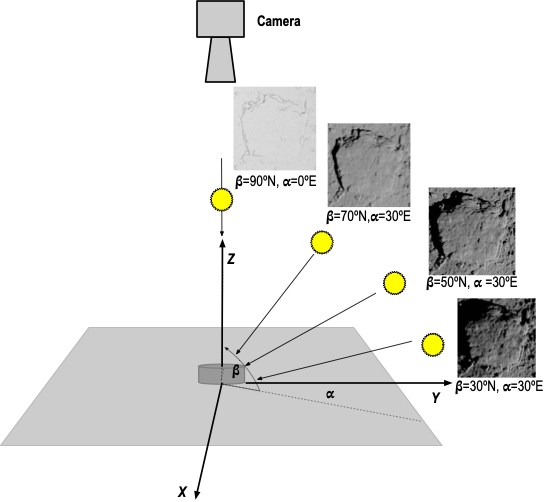
Figure 1. Setup used for rendering surface boulders observed by OLA on Bennu. Camera is looking straight down on surface with an elevation on 90°
Methodology:
In this analysis, each local boulder DTM had its slope de-trended, such that the boulder was sitting on a flat-horizontal plane. Images of the boulder were rendered using a ray tracing algorithm and a modified Lommel-Seeliger photometric function identical to what was done in Daly et al., (2022). The camera was always placed at an elevation angle of 90° (0° emission) and a range of 1 km from the surface, looking directly down at the boulder (Figure 1). The modeled camera had 1024x1024 pixels with a focal length of 500 mm and an instantaneous field of view (IFoV) of 4x10⁵ radians, resulting in images with a ground sample distance of 4 cm/px. These camera properties were picked so that the resulting image pixel scales were similar to the GSD of the DTMs. The boulder DTMs were rendered using a range of solar azimuths (α of 0° to 360°) and elevations (β -30° to 30° via 90°) (Figure 2). Images were rendered every 30° in α and 20° in β.

Figure 2. Boulder images rendered for differing sun azimuths α and elevations β. The image with the yellow outline indicates the observing conditions that existed during the DART impact (Daly et al., 2023).
Members of our team were then tasked with mapping lineaments on a subset of the synthetic images. Each investigator was only given images for one lighting condition when they undertook their lineament assessment, in order to minimize any bias that might have arisen by having more than one viewing orientation. They were also given a downsampled and smoothed version of the boulder DTM so that they could map lineaments on the rendered images in the Small Body Mapping Tool (SBMT, Ernst et al. 2018) if they so desired. Once all the rendered images were mapped and the result turned in, each investigator was given a full resolution boulder DTM with all of its renderings, so that a complete set of lineaments could be identified. These were then compared to the lineaments obtained from the individual rendered images. The results for any biases were then assessed.
Preliminary results:
The mapping is ongoing, and a full report of our findings will be presented at EPSC 2024. However, some preliminary findings can be mentioned. As is already well-known, the morphology of surface features, including boulder fractures, are not easily recognized when the sun elevation is high (immediately overhead): features get washed out. Images taken with low sun β (<20°) are also problematic because shadows hide any significant morphology. The best viewing geometry for finding boulder fractures seems to be between 20°< β <60° solar elevation. Using two orthogonal solar azimuths further reduce bias.
For lighting at the DART impact site (where the Sun was at about β = 30° and α= 10°), many of the fractures present on boulders can probably be identified. Cracks that are orientated in N-S, NE-SW and NW-SE are easily identifiable. Some E-W fractures could be missed.
Conclusion:
Lighting needs to be considered when evaluating orientation of boulder fractures. Biases related to lighting geometries may have implications for past fracture studies on Bennu and elsewhere. The evidence used to establish the importance of thermal fatigue operating on asteroids may need to be re-evaluated.
Acknowledgemnet: O.S.B and R.-L.B. are funded by NASA New Frontiers Data Analysis Program grant number 80NSSC22K1035.
References:
Buczkowski, D.L., Barnouin, O.S., Prockter, L.M., 2008. 433 Eros lineaments: Global mapping and analysis. Icarus 193, 39–52.
Daly, M.G., Barnouin, O.S., Dickinson, et al., 2017. The OSIRIS-REx Laser Altimeter (OLA) Investigation and Instrument. Space Science Reviews 212, 899–924.
Daly, M.G., Barnouin, O.S., Seabrook, J.A. et al.., 2020. Hemispherical differences in the shape and topography of asteroid (101955) Bennu. Science Advances 6. https://doi.org/10.1126/sciadv.abd3649
Daly, R.T., Ernst, C.M., Barnouin, O.S., et al., 2023. Successful Kinetic Impact into an Asteroid for Planetary Defense. Nature 1–3.
Daly, R.T., Ernst, C.M., Barnouin, O.S., et al., 2022. Shape Modeling of Dimorphos for the Double Asteroid Redirection Test (DART). Planet. Sci. J. 3, 207.
Delbo, M., Libourel, G., Wilkerson, J., et al., 2014. Thermal fatigue as the origin of regolith on small asteroids. Nature 508, 233–236.
Ernst, C.M., Barnouin, O.S., Daly, R.T., et al. 2018. The Small Body Mapping Tool (SBMT) for Accessing, Visualizing, and Analyzing Spacecraft Data in Three Dimensions, LPSC 48, abstract 1043.
Molaro, J.L., Walsh, K.J., Jawin, et al., 2020. In situ evidence of thermally induced rock breakdown widespread on Bennu’s surface. Nature Communications 1–11.
Lucchetti, A., Cambioni, S., Nakano, R. et al., 2024. Fast boulder fracturing by thermal fatigue detected on stony asteroids. Nature Communications, accepted.
How to cite: Barnouin, O., Ballouz, R., Lucchetti, A., Ernst, C., Parro, L., Kinczyk, M., Daly, T., Pajola, M., and Tusberti, F.: Fractures on Asteroid Boulders: Understanding Orientation Biases Caused by Lighting , Europlanet Science Congress 2024, Berlin, Germany, 8–13 Sep 2024, EPSC2024-555, https://doi.org/10.5194/epsc2024-555, 2024.
Interpreting the surface composition of the Moon and other airless bodies relies heavily on spectroscopic techniques spanning visible and near-infrared wavelengths. This study employed an integrated spectroscopy approach to measure and characterize a suite of lunar rock samples, a lunar meteorite, and lunar minerals. The primary objective was to demonstrate the methodology for building a robust spectral library that can support the interpretation of data from future lunar missions focused on understanding surface compositions and resource potential.
The analog samples characterized included 15 lunar mineral endmembers (pigeonite, augite, ilmenite, orthopyroxenes, olivine, anorthite, and bytownite), an Apollo 16 regolith sample (62231.44), and the Tisserlitine 001 lunar meteorite. These materials were prepared as fine powders sieved to grain sizes ranging from 25 to 125 micrometers. Spectroscopic measurements were performed under vacuum conditions using the state-of-the-art Bruker Vertex 80V FTIR instruments at the Planetary Spectroscopy Laboratory. Bidirectional reflectance spectroscopy was employed to acquire spectra at illumination angles of 30° and 45° relative to the sample surface normal, utilizing attached visible and near-infrared detectors. Hemispherical reflectance measurements were conducted to collect visible and near-infrared spectra separately, using integrating spheres. The calibrated hemispherical reflectance spectrum for the Apollo 16 sample exhibits a clear hydroxyl group feature near 3 micrometers, consistent with previous observations. Despite originating from different locations, the Apollo 16 lunar sample and the Tisserlitine 001 lunar meteorite displayed striking similarities in their visible and near-infrared bidirectional reflectance spectra, exhibiting absorption features characteristic of lunar highland compositions, including broad 1 and 2 micrometer bands indicating the presence of pyroxenes. However, the Tisserlitine 001 sample had slightly more pronounced pyroxene bands, although the overall spectral shape and absorption features were comparable between the two samples.
Further spectral analysis revealed notable observations. Ilmenite exhibited the highest overall reflectance, followed by orthopyroxene and pigeonite, while anorthite and bytownite displayed relatively low reflectance across most wavelengths. Olivine exhibited a distinct 10 micrometer absorption feature. Interestingly, the Tisserlitine 001 lunar meteorite displayed a unique spectral signature distinct from the other minerals studied. The study's findings contribute to developing a robust spectral library to aid in identifying lunar mineralogy and chemistry from orbital or landed measurements, enabling assessments of resource potential and improving understanding of lunar formation processes.
How to cite: Tripathi, P., Maturilli, A., and Alemanno, G.: Characterizing Lunar Materials: Spectral Analysis of Apollo 16 and Lunar Meteorite, Europlanet Science Congress 2024, Berlin, Germany, 8–13 Sep 2024, EPSC2024-668, https://doi.org/10.5194/epsc2024-668, 2024.
The Gaia Data Release 3 (DR3) contains high-precision sparse-in-time photometric data of more than 150 000 asteroids and spectroscopy of more than 60 000 asteroids (Tanga et al., A&A, 674, A12, 2023). We have fitted simple triaxial and general convex shapes to estimate the rotational periods, spin axes, and linear photometric slopes of the asteroids with the lightcurve inversion algorithm developed by Muinonen et al. (A&A, 642, A138, 2020). Sample selection of the asteroids follows Cellino et al. (A&A, in press, 2024), and we use the ellipsoid results from their genetic evolution algorithm to initiate our ellipsoid and convex shape inversion solutions.
In total, we have modelled linear photometric slopes for 8660 asteroids, which have at least 25 Gaia observations (MacLennan et al., in preparation). The slopes are used to compute H,G1,G2 phase functions (Muinonen et al., Icarus, 209, 542, 2010) to derive absolute magnitudes for the asteroids. As the absolute magnitudes have been calculated using Gaia’s G-band, they account for a larger portion of the incident solar spectrum compared to e.g. V-band. This is particularly useful for estimating the amount of absorbed sunlight for thermal infrared studies of asteroids via calculation of the Bond albedo.
Selecting the asteroids for which there are spectroscopic data as well, gives us 2381 asteroids to analyse further. We have kept the data from the Gaia red and blue photometers (RP and BP) separate due to problems merging them. The wavelength range of both ends have also been cut to eliminate unreliable behaviour in the spectra. We are left with the following wavelengths: 418, 462, 506, 550, 594 nm (in the BP), and 638, 682, 726, 770 nm (in the RP).
We have taken asteroid diameters from NASA’s NEOWISE survey (Mainzer et al., NEOWISE Diameters and Albedos V2.0, 2019) and the absolute magnitudes derived from the lightcurve inversion to calculate geometric albedos for the asteroids. Bond albedos are calculated from the geometric albedo and using the phase integral, q(G1,G2), from Muinonen et al. (Icarus, 209, 542, 2010). Traditionally, geometric albedos have been used to examine the inclusion of asteroids in asteroid families (Masiero et al., ApJ, 770, 7, 2013). Yet, taken together with the mean photometric slope of the families there seems to be a steep inverse linear trend with slopes smaller than 2 mag/rad at α = 20◦.
We now investigate the parameters further by creating bins of the photometric slope and geometric albedo pair using Principal Component Analysis (PCA) on the data of individual asteroids. The asteroid spectra within the bins are examined in order to evaluate how well the parameter pair aids in the classification of asteroids.
How to cite: Pentikäinen, H., MacLennan, E., Uvarova, E., Muinonen, K., Penttilä, A., Wilawer, E., Oszkiewicz, D., Cellino, A., Tanga, P., Wang, X., and Virkki, A.: Asteroid photometric and spectroscopic studies with Gaia DR3 data, Europlanet Science Congress 2024, Berlin, Germany, 8–13 Sep 2024, EPSC2024-894, https://doi.org/10.5194/epsc2024-894, 2024.
Introduction
The quantitative estimation of volumetric abundance of powder mixture is the basis of quantitative remote sensing analysis. Here we propose to analyze a unique laboratory measurements set, with precise composition, grain size and volumetric abundance.
We first propose a method to estimate the optical constant of materials, knowing the pure endmember spectra and their grain size. Then, we propose a method to transfer the measurement uncertainties to the volumetric abundance, based on the Bayesian approach and the full Hapke radiative transfer model. Using this approach, we are able to estimate grain size, volumetric abundance, and surface roughness.
The results show that this approach is able to well estimate the correct volumetric abundance with an uncertainty of 23% and grain size with a ratio uncertainty of 3.0, i.e. uncertainties in log10(grain size)=0.48. The numerical cost of the MCMC is quite large (a few minutes per spectra) but still reasonable to treat a hyperspectral image with the gain of robust handling of non-linearities and propagating the uncertainties.
Data
We used the laboratory data set containing 63 spectra, including 14 pure mineral powders and 49 binary mixtures of mineral powders (Koirala et al., 2021). These mixtures were created using 5 selected pure mineral powders: Aluminum oxide (Al2O3), Calcium oxide (CaO), Iron oxide (Fe2O33), Silicon dioxide (SiO2), and Titanium dioxide (TiO2). All mineral powders have a white color in the visible (except for Iron oxide which is red). Furthermore, they vary in densities and grain sizes. Although there are 10 possible combinations of these powders, due to experimental constraints the dataset contains exclusively seven binary mixture combinations of minerals namely: Al2O3-SiO2 (Al-Si), CaO-SiO2 (Ca-Si), CaO-TiO2 (Ca-Ti), Fe2O3-Al2O3 (Fe-Al), Fe2O3-CaO (Fe-Ca), Fe2O3 SiO2 (Fe-Si), and SiO2-TiO2 (Si-Ti). The provided dataset is particularly difficult to handle, without renormalization since several measurements of the same pure endmember are reproduced with a significant absolute level variability (see Figure 1).
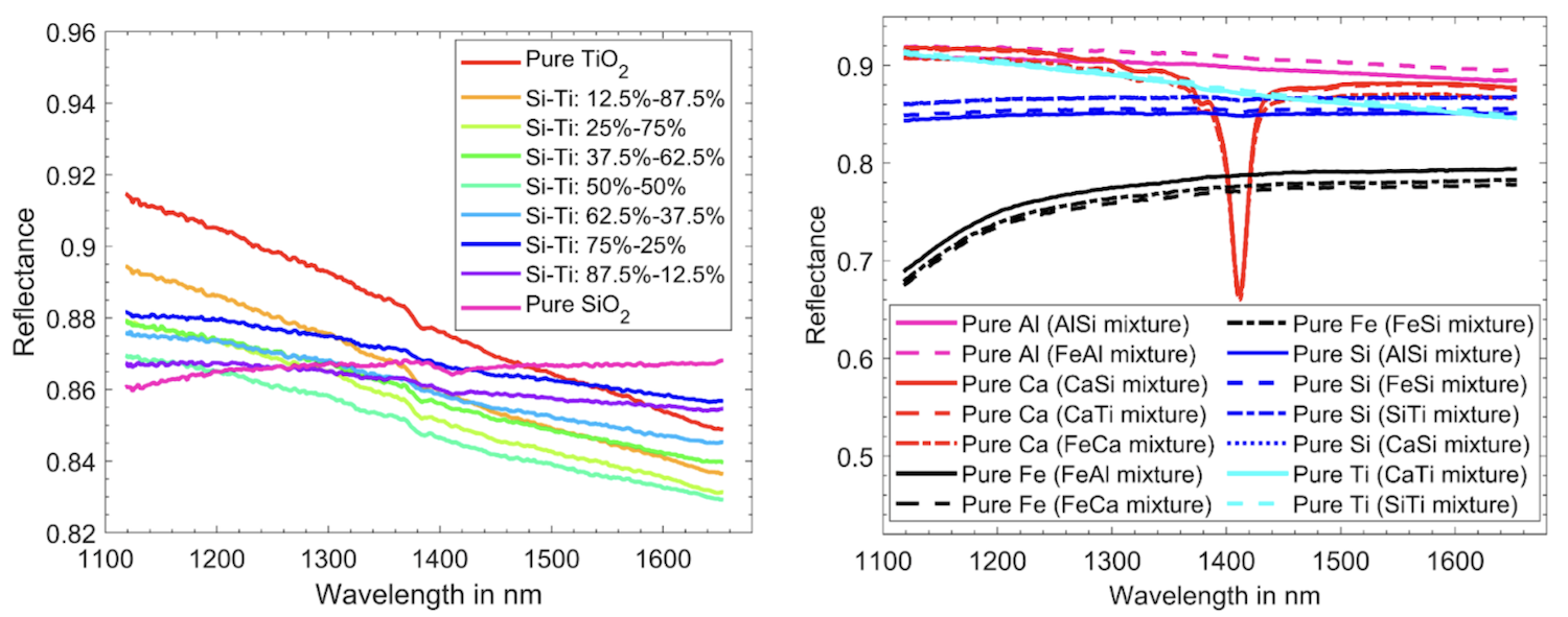
Figure 1 : Spectra of binary granular material mixtures. (left) example of binary mixture Si-Ti (right) Several observation of the same endmembers.
Method
We used the semi-analytical reflectance model from (Hapke, 2012), which is a good compromise between physical realism and efficient computation time. In Andrieu et al., 2022, we demonstrated that the usual gradient-descent method is not helpful because the non-linearities are so strong that the results mainly depend on the initialization. So the analysis is done by a Monte Carlo Bayesian approach to propagate the uncertainties from the measurement in reflectance to the parameters (Cruz Mermy et al., 2023). This operation is sometimes called inversion or assimilation.
Results
Figure 2 presents a typical result. This particular one is for a CaSi mixture with XCa=57.0%. The best fit is extremely close to the real observation. In addition, due to the uncertainties on the reflectance spectra, a range of solutions is acceptable. Figure 3 shows the corresponding posterior PDF for the four parameters that are unknowns: roughness θ0, volumetric proportion of XCa, grains size log10(DCa) and log10(DSi). All marginal PDFs are well constrained with a bell shape, except the log10(DSi) which is less constrained. The bivariate PDF indicates the relationship between the parameters. For instance, roughness seems highly correlated with the XCa.
Figure 3 shows the estimation of the abundance for the Al-Si mixture case. It shows that the trend is well reproduced in all cases. The global RMS is 23.0% for proportions X and 48.9% for log10(D). When the grain size is known, the RMS for X reduces to 21.1%.
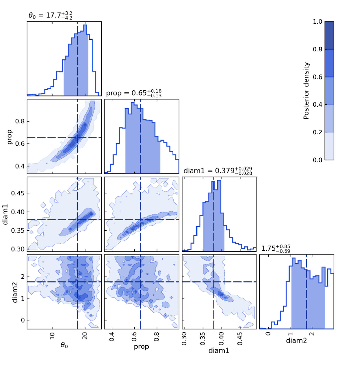
Figure 2 : Posterior PDF of the same case as Fig. 2 for the four unknown parameters: roughness θ0, volumetric proportion of XCa, grains size log10(DCa) and log10(DSi). The median values are indicated by a dashed line.
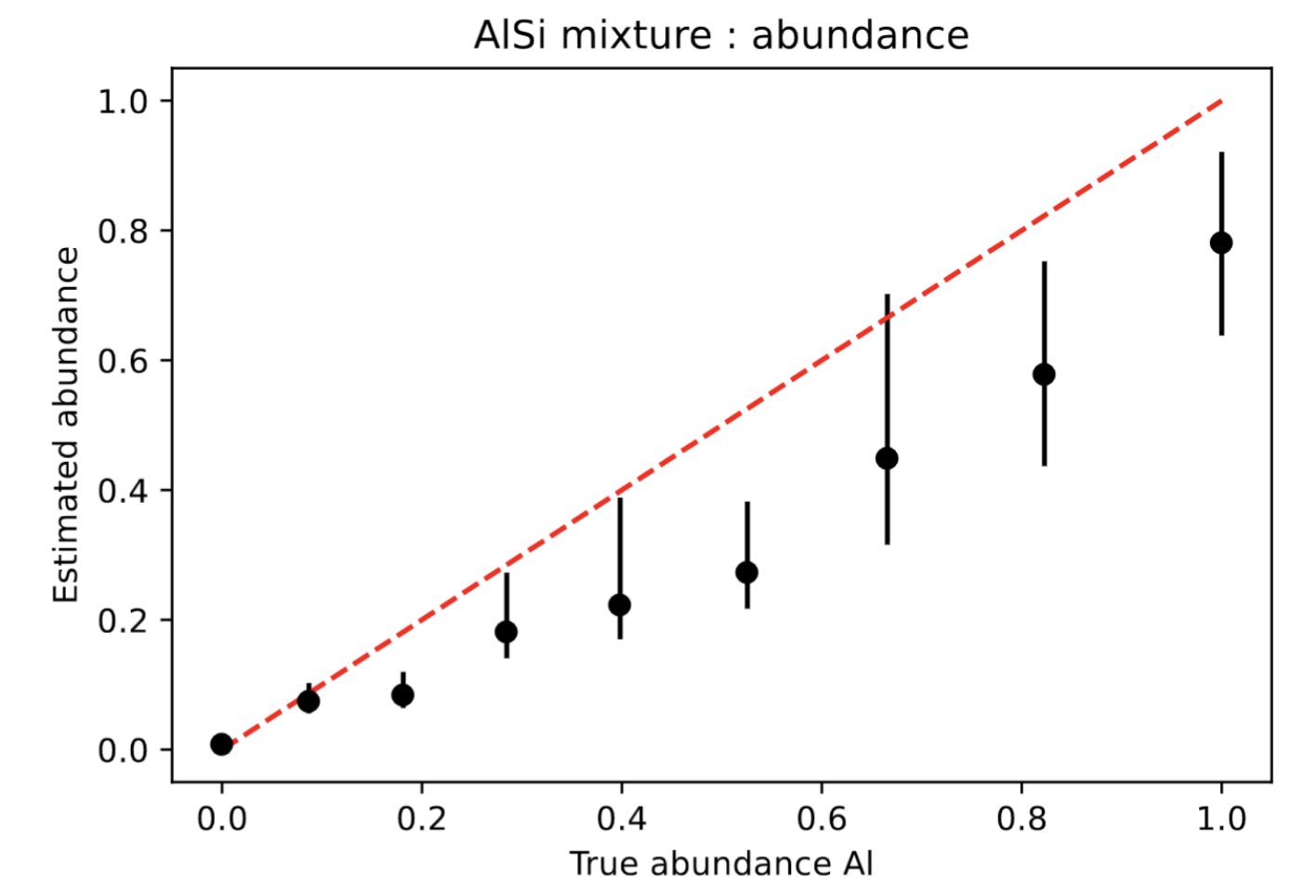
Figure 3 : True versus estimated volumetric abundance for all binary mixtures, estimating the four following parameters: roughness θ0, volumetric proportion X, grains sizes. The median and the 68.3% quantiles are plotted as the error bar.
Conclusion and perspective
We proposed a methodology to characterize powder samples from the shortwave infrared reflectance dataset (Schmidt et al., 2024). The methodology does not require the optical constant but only pure endmember spectra. In real remote sensing data, this is often not present in the scene. It may be possible to estimate endmembers by utilizing blind spectral unmixing methods such as the one presented in Ceamanos et al., 2011. Of course, if the optical constants are available, this first step can be bypassed.
Interestingly, the knowledge of the grain size does not help much to constraint the abundance due to the absolute level uncertainties due to absolute level uncertainties (see Fig. 1 right). This effect is difficult to handle in the lab, due to variability in roughness, compaction, illumination condition, calibration and should be even more difficult for real data.
Reference
Andrieu, F. Schmidt, G. Cruz-Mermy, I. Belgacem, and T. Cornet, Benchmarking Bayesian methods for spectroscopy,” in European Planetary Science Congress, Sep. 2022, pp. EPSC2022–502.
Bioucas-Dias, J.; Plaza, A.; Dobigeon, N.; Parente, M.; Du, Q.; Gader, P. & Chanussot, J. Hyperspectral Unmixing Overview: Geometrical, Statistical, and Sparse Regression-Based Approaches Selected Topics in Applied Earth Observations and Remote Sensing, IEEE Journal of, 2012, 5, 354-379,
Ceamanos, X.; Doute, S.; Luo, B.; Schmidt, F.; Jouannic, G. & Chanussot, J. Intercomparison and Validation of Techniques for Spectral Unmixing of Hyperspectral Images: A Planetary Case Study Geoscience and Remote Sensing, IEEE Transactions on, 2011, 49, 4341-4358, http://dx.doi.org/10.1109/TGRS.2011.2140377
Cruz Mermy, G.; Schmidt, F.; Andrieu, F.; Cornet, T.; Belgacem, I. & Altobelli, N. Selection of chemical species for Europa's surface using Galileo/NIMS Icarus, Elsevier BV, 2023, 115379, http://dx.doi.org/10.1016/j.icarus.2022.115379
Hapke, Theory of Reflectance and Emittance Spectroscopy, 2nd ed, Cambridge University Press, 2012.
Koirala, B.; Zahiri, Z.; Lamberti, A. & Scheunders, P. Robust Supervised Method for Nonlinear Spectral Unmixing Accounting for Endmember Variability IEEE Transactions on Geoscience and Remote Sensing, Institute of Electrical and Electronics Engineers (IEEE), 2021, 59, 7434-7448, http://dx.doi.org/10.1109/tgrs.2020.3031012
Schmidt, F.; Koirala, B., Andrieu, F., Determination of volumetric abundance of intimate mixture using Bayesian MCMC, 2024, under review in IEEE Sensor
How to cite: Schmidt, F., Koirala, B., and Andrieu, F.: Validation of abundance determination of granular mixture using radiative transfer and Bayesian MCMC, Europlanet Science Congress 2024, Berlin, Germany, 8–13 Sep 2024, EPSC2024-902, https://doi.org/10.5194/epsc2024-902, 2024.
I. Introduction
The JUpiter ICy Moons Explorer (JUICE) is a mission funded and led by the
European Space Agency (ESA) in the context of its Cosmic Vision program.
The Japanese space agency (JAXA) and the United States' NASA contributed to
this mission. The spacecraft carries 11 instruments designed to observe and
monitor the Jupiter system, with a focus on the Galilean moons Callisto,
Europe and Ganymede, in the intent of furthering our present knowledge of
the Solar System and our understanding of planetary formations, two key
themes of the Cosmic Vision programi [1].
We will present the program (GeoMAJIS) we designed, developed and deployed
to help with the interpretation of JUICE's visible and infrared spectrometer
(MAJIS) observations.
II. The MAJIS spectrometer
MAJIS is a push-broom imaging spectrometer designed to observe the atmosphere
of Jupiter and characterize the surface of its moons from the visible to the
thermal infrared domains (.4 - 5.6 µm) [1]. This instrument has two channels
sharing the same field-of-view (FOV), each equipped with a Teledyne H1RG
1024x1024 detector, with one optimised for the 0.4-2.35 µm domain (VISNIR)
and the other for the 2.25-5.6 µm domain (IR). The detectors are composed
of squared pixels with an instantaneous FOV of 75 µrad. In the baseline mode, a x2
binning is applied on each detector to increase the signal, such that the FOV
is provided by a 1x400 binned pixels segment, i.e. a 8.5°x10-3*3.43° window.
When orbiting Jupiter from a distance of 10^6 km (or Ganymede at 500 km),
MAJIS' spatial resolution will be of 150 km/pxl (respectively 75 m/pxl).
The instrument also possesses a mirror which allows to shift its FOV in
the along-track axis by up to 2° in either direction.
As MAJIS will perform in a complex observational context, in which
occultations are common, it is necessary to complement the calibrated
observations with ancillary data to ease their interpretation.
III. The GeoMAJIS code
This program relies on the CSPICE library [3] to
perform the necessary computations to detail the observational context,
based on the spacecraft' predicted (or recomputed) trajectory and
attitude, as well as celestial bodies' ephemerides.
GeoMAJIS details for instance which objects are present in MAJIS' FOV,
their state (i.e position and velocity) with respect to different inertial
frames, the Sun's and its own position relative to them, and the
instrument' spatial resolution at their surface.
In addition, the program also performs ray-tracing computation specific
to each observation so that for each pixel, it might be known which
surface element of which object was observed, if it was fully illuminated
and visible, or shadowed or occulted from the spacecraft's perspective.
Such computations are performed either with a simple ellipsoidal
representation of the observed bodies, or, when available, also with
a detailled 3D model of the target.
All the results of the RTX computations are then written-out as a
multiple-frame FITS file, while the other results are written down into
the geometry dictionary of the PDS4 descriptor of the said FITS file,
complementing the corresponding scientific observation.
IV. The August 2024 Earth flyby
In complement to theoretical simulations, the GeoMAJIS program will be
tested and perfected in the shadow of the 20th of August 2024 Earth
flyby. While presently available ephemerids allow to simulate this
flyby, as illustrated by Fig. 1.

Fig. 1: 2D plot of the Local Time at the surface of the Earth, according the predicted trajectory of the JUICE spacecraft at the present time.
The plot depicts the simulation results of 196 acquisitions with the VISNIR channel (one every 15 minutes, vertical axis) taken with 400 pixels (horizontal axis).
As one can understand from the results of Fig.1, during this flyby, the spacecraft ingresses the Earth system in the shadow of the Earth and makes its egress while imaging most of the day-side and part of the evening-side terminator. The local time was evaluated and corrected by the sun's elevation with respects to the local normals of the surface.
Given the suite of instruments aboard the spacecraft, the reconstructed trajectory of the spacecraft will be computed with at best a sub-meter accuracy.
Such accuracy will allow to compare and find-out any differences between simulations and observations that might be due either to a theoretical
or a factual origin.
These efforts will constitute a new evaluatory review of the program and its algorithm and any correction will be included in the eventual updated version of the calibration pipeline.
V. Conclusions
We designed, developped and tested a segment of MAJIS' calibration pipeline. This segment aims at providing the most complete description of the
observational context of the varied MAJIS acquisitions.
We shall present the algorithm of this program, as well as the results of present simulations of observations in the Jupiter system as well as the preliminary
results from the review of the August 2024 Earth flyby.
References:
- 1. Grasset et al., PSS, http://dx.doi.org/10.1016/j.pss.2012.12.002
- 2: Acton et al., Planet. Space Sci.. Vol. 44, No. 1, pp. 65-70. 1996
How to cite: Feller, C., Sophie, J., and Cédric, L.: GeoMAJIS, providing the observational context for the JUICE/MAJIS spectrometer, Europlanet Science Congress 2024, Berlin, Germany, 8–13 Sep 2024, EPSC2024-1073, https://doi.org/10.5194/epsc2024-1073, 2024.
Asteroids are diverse objects found in the Solar System, populating in large numbers the near-Earth space, yet most of them form the main belt. While upcoming observatories promise frequent observations of asteroids to compute their orbit, understanding their physical composition remains a challenge due to the inherent difficulty in obtaining spectra.
Launched in 2013, GAIA satellite repeatedly scans the entire sky, not only mapping the more than 1 billion stars, but also discover and measure exoplanets, asteroids, comets and planetary satellites in our Solar System. For the asteroids and comets, GAIA provides more accurate astrometry, photometry as well as albedo and spectra.
In this study we accessed the freely available GAIA Solar System Objects reflectance spectra in the visible range (418-990 nm) and built a catalogue of their spectral wavelengths. After thresholding for the well calibrated spectras we tested 8 unsupervised machine learning (ML) models to cluster the spectras into classes.
After fine hyperparameter tuning of the models we found that several ML methods capture well the features of the already classified asteroids. Also, we obtained a spectral classification for the unclassified asteroids observed by GAIA.
The next step is to extend the study by employing the dynamical features and the albedo to better constrain the asteroid families, and ultimately, to understand distribution of the asteroids in the Solar System.
Acknowledgements: SA was supported during this work by the ESA Archival Research Visitor Programme.
How to cite: Anghel, S., Merin, B., and Kueppers, M.: Asteroid Classification with GAIA: Machine Learning Insights from Reflectance Spectra, Europlanet Science Congress 2024, Berlin, Germany, 8–13 Sep 2024, EPSC2024-1096, https://doi.org/10.5194/epsc2024-1096, 2024.
Abstract:
Understanding the thermal properties of comets, asteroids, and icy moons is crucial for advancing our knowledge of their composition and evolution. An increasing number of missions to these bodies, including Rosetta, Osiris-Rex, Europa Clipper, and JUICE, necessitate thermal models that accurately consider their complex topographies.
We have developed a Python model that predicts diurnal temperature variations on airless bodies in three dimensions, factoring in their morphologies. This model significantly improves simulation accuracy by incorporating shadowing effects. The results are consistent with established models such as the one-dimensional thermal conduction model of J.R. Spencer, thermprojrs [1], and the three-dimensional surface energy balance model by Guilbert-Lepoutre & Jewitt [2].
Our tool was built to support missions such as the NASA Lucy Mission and the ESA Comet Interceptor mission. However, it is suited to a wide range of targets, including those with active surfaces. The model is user-friendly and operates quickly, running in seconds for basic shape models, and requiring only a few minutes for a shape model of comet 67P with 16,000 facets. It is designed to handle subsurface heating efficiently and is parallelised, enabling applications to large, high spatial resolution shape models.
Background:
The thermal behaviour of airless planetary bodies is governed by their surface and subsurface properties, including albedo, surface roughness, and thermal inertia. Accurate thermal models are essential for interpreting observational data and planning missions. Traditional models, such as Spencer's thermprojrs, have provided valuable insights into the thermal evolution of these bodies by simulating one-dimensional heat conduction. These models are instrumental in understanding the diurnal and seasonal temperature variations on the surface.
However, the complexity of three-dimensional topographic features, such as craters, ridges, and boulders, necessitates more advanced modelling techniques. While existing three-dimensional models have addressed some of these complexities, there remains a need for accessible, high-resolution models to simulate and interpret thermal data from current and upcoming missions accurately.
Outline of the Model:
Our open-source Python-based model aims to fill this gap by providing a comprehensive tool that can account for three-dimensional morphological features and shadowing effects. This model enhances the accuracy of temperature predictions and makes advanced thermal modelling techniques available to a wider scientific community. The integration of this model with thermal mapping data from missions can further refine shape models, leading to improved interpretations of the thermal properties of airless bodies.
The model solves a surface energy balance equation for each facet of the shape model file. This equation factors in solar heating, radiative loss, thermal conduction, and subsurface heating. The result is a temperature map that evolves over time, providing insights into the diurnal cycle and the thermal properties of the target body under various conditions.
This approach is efficient and user-friendly, requiring only a few minutes to process a shape model with thousands of facets. The model's parallelised nature allows for rapid computation, making it suitable for extensive simulations and analyses.
Validation Work:
To validate our model, we compared its output with the results from Spencer's one-dimensional model. As shown in Figure 1, the temperature versus time profiles from both models show close agreement, with slight differences attributed to the handling of deep layer temperatures.

Figure 1: Temperature vs Time for a single facet. Comparison between Spencer model and our model.
The model has been tested on various shape models, including comet 67P and the asteroid Bennu. The inclusion of shadowing effects, enhances the accuracy of temperature predictions in areas with significant topographic variation (Figure 2).
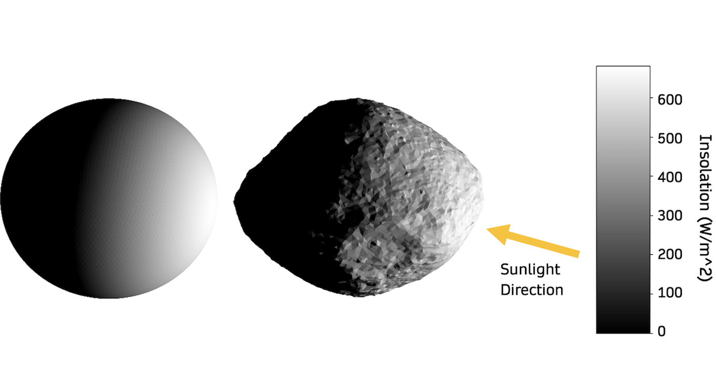
Figure 2: 3D illumination model with shadowing effects for shape models of a sphere, Bennu, and 67P.
The thermal map generated by our model (Figure 3), highlights the temperature distribution across the surface. These maps are essential for understanding the thermal evolution of the target bodies and planning mission operations. This model could also be used in tandem with thermal mapping data from missions to refine shape models, enhancing the accuracy of the thermal simulations and providing more detailed insights into the surface properties of the target bodies.
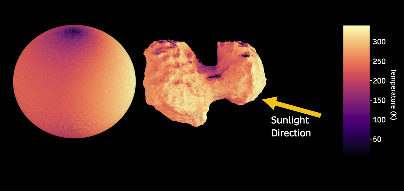
Figure 3: Thermal map showing temperature distribution on a sphere, Bennu, and 67P.
Conclusion:
Our open-source Python model represents an improvement in the simulation of thermal behaviour on airless planetary bodies. It provides accurate temperature predictions by incorporating three-dimensional surface features and shadowing effects. The model runs efficiently and can be parallelised, making it suitable for a wide range of applications, including realistic instrument simulations and mission planning.
Planned improvements to the model include implementing radiative self-heating, scattering of incident light, and energy loss through sublimation. Extensive parameter sensitivity analysis will further enhance the model's applicability to diverse targets.
The code is open source, and contributions are welcome:
github.com/duncanLyster/comet_nucleus_model
References:
- Spencer, J.R., Lebofsky, L.A., and Sykes, M.V., 1989. Systematic biases in radiometric diameter determinations. Icarus, 78(2), pp.337-354.
- Guilbert-Lepoutre, A., and Jewitt, D., 2011. Thermal shadows and compositional structure in comet nuclei. The Astrophysical Journal, 743(1), p.31.
How to cite: Lyster, D., Howett, C., and Penn, J.: Predicting Surface Temperatures on Airless Bodies: An Open-Source Python Tool, Europlanet Science Congress 2024, Berlin, Germany, 8–13 Sep 2024, EPSC2024-1121, https://doi.org/10.5194/epsc2024-1121, 2024.
Please decide on your access
Please use the buttons below to download the supplementary material or to visit the external website where the presentation is linked. Regarding the external link, please note that Copernicus Meetings cannot accept any liability for the content and the website you will visit.
Forward to presentation link
You are going to open an external link to the presentation as indicated by the authors. Copernicus Meetings cannot accept any liability for the content and the website you will visit.
We are sorry, but presentations are only available for users who registered for the conference. Thank you.
Please decide on your access
Please use the buttons below to download the supplementary material or to visit the external website where the presentation is linked. Regarding the external link, please note that Copernicus Meetings cannot accept any liability for the content and the website you will visit.
Forward to session asset
You are going to open an external link to the asset as indicated by the session. Copernicus Meetings cannot accept any liability for the content and the website you will visit.
We are sorry, but presentations are only available for users who registered for the conference. Thank you.