OPS5 | Exploration of Titan

OPS5

Exploration of Titan
Co-organized by MITM
Conveners: Audrey Chatain, Thomas Gautier | Co-conveners: Sandrine Vinatier, Nicholas Teanby, Bruno de Batz de Trenquelléon, Robin Sultana, Lucy Wright
Orals FRI1
| Fri, 11 Sep, 08:30–10:00 (CEST)|Room Jupiter (Jazz 1 & 2)
Orals FRI2
| Fri, 11 Sep, 11:00–12:30 (CEST)|Room Jupiter (Jazz 1 & 2)
Posters THU-POS
| Attendance Thu, 10 Sep, 18:00–19:30 (CEST) | Display Thu, 10 Sep, 08:30–19:30|Foyer 3, F3.11–14
Fri, 08:30
Fri, 11:00
Thu, 18:00
Saturn's moon Titan, despite its satellite status, has nothing to envy the planets: it has planetary dimensions, a substantial and dynamic atmosphere, a carbon cycle, a variety of geological features (dunes, lakes, rivers, mountains and more), seasons, and a potential hidden ocean. It even now has its own mission: Dragonfly, selected by NASA in the frame of the New Frontiers program. In this session, scientific presentations are solicited to cover all aspects of current research on Titan: from its interior to its upper atmosphere, using data collected from the Cassini-Huygens mission (2004-2017) and/or from telescopes (e.g., ALMA, JWST) and/or based on modelling and experimental efforts to support the interpretation of past and future observations of this unique world.

Orals FRI1: Fri, 11 Sep, 08:30–10:00 | Room Jupiter (Jazz 1 & 2)

Chairpersons: Thomas Gautier, Lucy Wright
08:30–08:33
Search for molecules in the atmosphere
08:33–08:45
|
EPSC2026-38
|
ECP
|
On-site presentation
Chiara Castagnoli, Bianca Maria Dinelli, Federico Fabiano, Manuel López Puertas, Leonardo Ronchini, Maya García Comas, and Bernd Funke

The Cassini–Huygens mission (2004–2017), covering nearly half a Titan year, provided an unprecedented dataset to investigate the seasonal variability of Titan’s upper atmosphere. The Visual and Infrared Mapping Spectrometer (VIMS) onboard Cassini enabled long-term monitoring of the poorly characterized upper atmosphere of Saturn’s largest moon, detecting strong infrared non-LTE emissions from key species, including CH₄, HCN, and C₂H₂, which serve as tracers of Titan’s atmospheric chemistry and dynamics.

This study builds on previous analysis of VIMS daytime infrared spectra acquired from 2004–2012 (Dinelli et al., 2019), which revealed clear seasonal variability in the abundance and distribution of these molecules during northern winter (2004-2009) and early spring (2010-1012) and suggested an extended meridional circulation reaching well above 500 km, possibly up to 750–800 km or higher.

Here, we extend the dataset to 2013–2017 to complete seasonal coverage through northern late spring and southern late autumn. The analysis focuses on the 2.9–3.4 µm range, probing altitudes from 500 to 1100 km, spanning the upper mesosphere and lower thermosphere. The results show large enhancements of HCN and C2H2 near 800 km at the south pole during southern late autumn, consistent with an extension of the middle atmosphere circulation above 500 km. At similar latitudes, enhanced CH4 concentrations are observed above 700 km, supporting the hypothesis that the meridional circulation may reach the lower thermosphere, although reduced photodissociation under weak autumn illumination might also contribute.

These results support a vertically extended meridional circulation, with subsidence over the winter pole linked to a north polar vortex and a subsequent reversal after its breakdown following the northern spring equinox.


References:

Dinelli, B.M., Puertas, M.L., Fabiano, F., Adriani, A., Moriconi, M.L., Funke, B., García-Comas, M., Oliva, F., D’Aversa, E., Filacchione, G., 2019. Climatology of CH4, HCN and C2H2 in Titan’s upper atmosphere from Cassini/VIMS observations. Icarus 331, 83–97. doi: 10.1016/j.icarus.2019.04.026


How to cite: Castagnoli, C., Dinelli, B. M., Fabiano, F., López Puertas, M., Ronchini, L., García Comas, M., and Funke, B.: Seasonal variations of CH4, HCN, and C2H2 in Titan’s upper atmosphere from 13 years of Cassini/VIMS observations, Europlanet Science Congress 2026, The Hague, The Netherlands, 7–11 Sep 2026, EPSC2026-38, https://doi.org/10.5194/epsc2026-38, 2026.

08:45–09:00
|
EPSC2026-706
|
ECP
|
On-site presentation
Joshua S. Ford, Nicholas A. Teanby, Conor A. Nixon, Patrick G.J. Irwin, Veronique Vuitton, and Lucy Wright

Introduction

Oxygen is the universes third most abundant element (Bergman et al. 2021) and is extremely rich in the Saturnian system (Feuchtgruber et al. 1997). Studies have found oxygen-bearing molecules and ions in Saturn’s atmosphere (Esposito et al. 2005) , in its plasma environment (Wilson et al. 2016) and on its moon Enceladus (Thomas et al. 2016). In contrast, Titan is scare in oxygen species, boasting a rich atmosphere of hydrocarbons and nitriles (Vuitton et al.2024) that interact uniquely, often consuming free oxygen or locking it away as water ice. This results in an anoxic, organic and diverse environment with little oxygen to terminate reactions (Nixon et al. 2024).

To date, only three oxygen-bearing molecules have been detected in Titan’s atmosphere: CO (Lutz et al. 1983), CO2 (Sameulson et al 1983) and H2O (Coustenis et al. 1997). These molecules form from externally delivered OH, O+  and/or H2O being photodissociated by solar UV and energetic particles in the upper atmosphere, before recombining and being transported downwards via atmospheric mixing (Vuitton et al. 2019).  Of the detected species, the least well-understood is water vapour. CO and CO2 have been studied extensively and exhibit little variation in latitude, time or altitude (Teanby et al. 2019). Yet, investigations into H2O have been limited to single measurements or large averages (Vuitton et al 2007,  Cui et al 2009, Cottini et al. 2012, Bauduin et al 2018). Its weak infrared emission lines and low atmospheric abundances make it difficult to model. Water plays a vital role in Titan’s atmosphere, distributing oxygen and acting as a tracer for atmospheric dynamics. Its chemical pathways may produce species important for astrobiology like formaldehyde (Nixon 2024).


Figure 1: Schematic showing the potential pathways of H2O and its transport through the atmosphere until condensation near the tropopause. Not all reactions have been included.. The chemistry shown is based on Vuitton et al. 2019 and Nixon 2024. Molecules in green denote those predicted by photochemical models but not yet been detected.

Method

Here, we present the first reported latitudinal and temporal variability of H2O in Titan’s atmosphere. Using the NEMESIS radiative transfer code (Irwin et al. 2008) with temperature a priori profiles from Teanby et al. 2019 and a vertical water a priori profile from Vuitton et al.2019, we retrieve water abundance in Titan’s stratosphere from 157 far-infrared high-resolution Cassini CIRS FIRNADCMP observations (Flasar et al. 2004) across the entire mission and moon. To improve the fit and account for variations in the baseline caused by aerosols, we fit scaled gaussian basis function (see associated EPSC 2026 poster for more information). Due to low signal-to-noise in some spectra and low abundances, 51 observations were averaged in 13 bins. Our derived column abundances are consistent with all previous measurements of water in Titan’s middle atmosphere, and the retrieved profiles show consistency with upper atmosphere upper limits derived from INMS (Vuitton et al. 2007, Cui et al 2009). These results provide important constraints for future photochemical models and GCM's, particularly those focused on oxygen chemistry and organic molecule formation. 

Results

At the poles, lower column abundances are observed due to reduced temperatures, which decrease the saturation vapour pressure. We also find high retrieved scale factors (applied to the a priori) at the north pole indicating that water is mildly enhanced by a factor of 3 relative to mid-latitudes similar to trace gases like HCN (Teanby et al. 2012), although much weaker. This is likely caused by water-rich air subsiding into the polar vortex, concentrating and adiabatically heating within the confines of the polar mixing boundary (Teanby et al. 2017). We find no evidence of seasonality, however we do find statistically significant time-variability at low-to-mid latitudes. Analysis of atmospheric residence times and comparison with the TAM GCM (Lombardo et al. 2023) shows the variability is not explained by photochemistry or atmospheric dynamics and may indicate a time-varying source. This idea was also previously suggested by Moreno et al. 2012 and Bauduin et al. 2018. We explore potential drivers of time-variability and conclude that short-term month-scale variations in Enceladus’ neutral torus, and Saturn’s dynamic magnetospheric environment could be responsible. The derived incoming OH flux needed to explain our results matches the calculated OH flux from the neutral torus, implying Enceladus could be the dominant source of Titan's water. 


Figure 2:  Step-by-step schematic showing the potential path of H2O (OH) molecules from Enceladus to Titan, highlighting consistency or variability at each step. Each band represents a different type of neutral torus and the dotted lines originating from Saturn represent the magnetic field.

References

Bauduin. A. et al. 2018. Icarus 301, 136–151. doi: 10.1016/j.icarus.2017.09.039. 

Bergman. M.  et al. 2021. Monthly Notices of the Royal Astronomical Society 508 (2). Doi: 10.1093/mnras/stab2160

Cottini. V. et al. 2012. Icarus 220 (2), 855–862. doi: 10.1016/j.icarus.2012.06.009. 

Coustenis. A. et al. 1998. A&A 336, 85-89.

Cui. J. et al. 2009. Icarus 200, 581–615. doi: 10.1016/j.icarus.2008.11.005. 

Esposity. L. et al. 2005. Science, 307 (5713). Doi: 10.1126/science.1105606

Feuchtgruber. H. et al. 1997. Nature 389, 159-162. Doi: 10.1038/38236

Flasar. F. M. et al. 2004. Space Science Reviews 115 (1–4), 169–297. doi: 10.1007/s11214-004-1454-9. 

Irwin, P. G. J. et al. 2008. Journal of Quantitative Spectroscopy and Radiative Transfer 109 (6), 1136–50. Doi: 10.1016/j.jqsrt.2007.11.006.

Lombardo. N.A. et al. 2023. JGR: Planets, 123. Doi: 10.1029/2023JE008061.

Lutz. B.L. et al. 1983. Science, 220 (4604), 1374-1375. Doi:10.1126/science.220.4604.1374.

Moreno. R. et al. 2012. Icarus 221, 753–767. 10.1016/j.icarus.2012.09.006

Nixon. C.A. 2024. ACS Earth Space Chem 29, 8(3), 406-456. Doi: 10.1021/acsearthspacechem.2c00041.

Samuelson. R. E. et al. 1983. JGR: Space Physics, 88(A11), 8709-8715. Doi: 10.1029/JA088iA11p08709.

Teanby. N.A. et al. 2012. Nature, 491, 732. Doi: 10.1038/nature11611

Teanby. N.A. et la. 2017. Nature Communications, 8, 1586.Doi:10.1038/s41467-017-01839-z

Teanby. N.A. et al. 2019. Geophysical Research Letters, 46, 3079-3089. Doi: 10.1029/2018GL081401.

Thomas. P.C. et al. 2016. Icarus, 264, 37-47. DOI: 10.1016/j.icarus.2015.08.037.

Wilson, R. et al. 2015. JGR Space Physics 120 (8). DOI:10.1002/2014JA020557.

Vuitton. V. et al. 2007. Icarus 191. doi: 10.1016/j.icarus.2007.01.028.

Vuitton.V. et al. 2019. Icarus, 324, 120-197. Doi: 10.1016/j.icarus.2018.06.013

Vuitton. V. et al. (2024), ‘Chapter 6 : Titan’s Atmospheric Structure, Composition, Haze, and Dynamics’ In Titan after Cassini–Huygens, COSPAR Scientific Symposium Series.


How to cite: Ford, J. S., Teanby, N. A., Nixon, C. A., Irwin, P. G. J., Vuitton, V., and Wright, L.: Time-variability and north pole enhancement of Titan’s atmospheric water abundance , Europlanet Science Congress 2026, The Hague, The Netherlands, 7–11 Sep 2026, EPSC2026-706, https://doi.org/10.5194/epsc2026-706, 2026.

09:00–09:12
|
EPSC2026-566
|
On-site presentation
Conor Nixon, Thomas Greathouse, and Keeyoon Sung

Saturn’s moon Titan is a ‘hydrocarbon heaven’. Its mildly reducing atmosphere, composed mostly of nitrogen (N2, ~95-97%), also possesses a significant amount of methane (CH4, ~5-2%). With a near-absence of atmospheric oxidizers, photochemistry acts on the methane and nitrogen to break up the simpler molecules, and results in a dizzying array of more complex organic chemicals: mostly hydrocarbons (CxHy) and nitriles (CxHyCN). To date, around two dozen molecules have been definitively identified using astronomical spectroscopy, while the presence of hundreds more has been inferred from photochemical models and low-resolution mass spectroscopy of atmospheric gases from Cassini/Huygens.

Further characterization of Titan’s atmospheric chemicals is important for multiple reasons: (i) investigating how pre-biotic chemistry occurs across different environments, to build up more complex species from simpler ingredients (e.g. Miller-Urey type synthesis); (ii) deciphering the origin and history of Titan’s atmosphere; (iii) understanding the feedback between Titan’s atmospheric chemistry, dynamics and weather; (iv) putting solar system bodies in the context of the emerging gallery of exoplanets, and building out the wider parameter space of possible planetary atmospheres.

To this end, we are undertaking astronomical searches for larger molecules on Titan than those known at present, focusing on undetected C3 and C4 hydrocarbons (Fig. 1). This will help to expand our knowledge of the atmospheric inventory and provide valuable constraints on photochemical models. The transition to C3 species and beyond is a critical juncture in organic chemistry. This marks the point where structural isomerism becomes possible, resulting in multiple species with the same chemical formula but different structures. Therefore, astronomical measurements become especially important for C3 species and beyond, as unit resolution mass spectroscopy encounters significant ambiguities.

We report on current progress in the search for C3 and C4 hydrocarbons using the high-resolution TEXES spectrometer on the NASA 3m IRTF telescope on Maunakea, HI, and the implications for knowledge of Titan’s chemistry. These results will provide key context for science planning and a data analysis for NASA’s upcoming Dragonfly mission to Titan, as well as for possible visits by an planned ESA L4 mission to the Saturn system.

Figure 1: Hydrocarbon chemical work for Titan’s atmosphere. Most small molecules (C1 to C2) are well studied and characterized, while C3 molecules are partially known, and C4 and larger species remain mostly undetected.


How to cite: Nixon, C., Greathouse, T., and Sung, K.: Searching for heavy hydrocarbons on Titan using infrared astronomy, Europlanet Science Congress 2026, The Hague, The Netherlands, 7–11 Sep 2026, EPSC2026-566, https://doi.org/10.5194/epsc2026-566, 2026.

The famous Titan hazes
09:12–09:24
|
EPSC2026-1056
|
ECP
|
On-site presentation
Nathan Le Guennic, Panayotis Lavvas, Tommi Koskinen, and Devin Hoover

Titan's organic haze is central to the moon's atmospheric energy balance and photochemistry, and are intimately tied to cloud formation and the broader chemical cycles operating in the stratosphere [1, 2, 3, 4]. Constraining haze properties is therefore essential to validate the theoretical models describing their formation and growth [5, 6].

Several Cassini instruments have been used to measure haze extinction, through stellar occultations with UVIS [7] and VIMS [8], thermal emission with CIRS [9], or direct imaging with ISS [10]. However, extinction alone cannot separate particle size from number density. Most studies have worked around this by fixing particle size to Huygens/DISR values [11], which are only representative of a single location and altitude range. ISS scattered-light observations have allowed both quantities to be retrieved simultaneously [12, 13] near the detached haze layer (around 500 km).

We present the latest results of our analysis of the Ultraviolet Imaging Spectrograph (UVIS) limb airglow observations, provided by the latest UVIS Python package (UPyP) [14]. We use multiple flyby data within the same terrestrial year to collect UV emission from scattering by haze particles in the 1600-1900 Å range, at different phase angles, to fit the phase function of aerosols at different altitudes that is sensitive to particle size. We limit our analysis to phase angles below 150° as observations at higher angles appear contaminated by instrumental effects.

The diversity of observations allows us to retrieve the haze particle size and number density at multiple altitudes, latitudes and times. The inversion procedure considers a spherical layer structure of the atmosphere, including the haze single-scattering, N2 rayleigh scattering, extinction by haze and gases, and airglow emission [15] depending on each observation geometry. At each altitude layer, the haze is represented by a log-normal size distribution with a mean radius set as a free parameter, and a number density set as a second free parameter. The two parameters are inverted using the maximum a-priori likelihood (MAP) [16]. The data is binned by latitude and local time to retrieve information at different latitudes and derive diurnal variations. The entire Cassini mission dataset is used to perform this analysis allowing us to retrieve the spatial and temporal evolution of the haze properties through out the mission.


References

[1] Courtin. "Aerosols on the Giant Planets and Titan". Space Science Reviews, 2005.

[2] Lavvas et al. "Condensation in Titan's Atmosphere at the Huygens Landing Site". Icarus, 2011.

[3] Larson et al. "Simulating Titan's Aerosols in a Three Dimensional General Circulation Model". Icarus, 2014.

[4] De Batz De Trenquelléon et al. "The New Titan Planetary Climate Model. II. Titan's Haze and Cloud Cycles". The Planetary Science Journal, 2025.

[5] Lavvas et al. "Surface Chemistry and Particle Shape: Processes for the Evolution of Aerosols in Titan's Atmosphere". The Astrophysical Journal, 2011.

[6] Lavvas et al. "Aerosol Growth in Titan's Ionosphere". Proceedings of the National Academy of Sciences, 2013.

[7] Koskinen et al. "The Mesosphere and Lower Thermosphere of Titan Revealed by Cassini/UVIS Stellar Occultations". Icarus, 2011.

[8] Bellucci et al. "Titan Solar Occultation Observed by Cassini/VIMS: Gas Absorption and Constraints on Aerosol Composition". Icarus, 2009.

[9] Vinatier et al. "Analysis of Cassini/CIRS Limb Spectra of Titan Acquired during the Nominal Mission II: Aerosol Extinction Profiles in the 600–1420 Cm-1 Spectral Range". Icarus, 2010.

[10] Seignovert et al. "Haze Seasonal Variations of Titan's Upper Atmosphere during the Cassini Mission". The Astrophysical Journal, 2021.

[11] Tomasko et al. "A Model of Titan's Aerosols Based on Measurements Made inside the Atmosphere". Planetary and Space Science, 2008.

[12] Seignovert et al. "Aerosols Optical Properties in Titan's Detached Haze Layer before the Equinox". Icarus, 2017.

[13] West et al. "The Seasonal Cycle of Titan's Detached Haze". Nature Astronomy, 2018.

[14] Le Guennic et al. "Methods for analysing low signal-to-noise emission observations: the Cassini Ultraviolet Imaging Spectrograph pipeline and application to Titan airglow observations". The Planetary Science Journal, 2026 (accepted).

[15] Lavvas et al. "N2 State Population in Titan's Atmosphere". Icarus, 2015.

[16] Rodgers. "Inverse Methods for Atmospheric Sounding: Theory and Practice". World Scientific, 2000.

How to cite: Le Guennic, N., Lavvas, P., Koskinen, T., and Hoover, D.: UVIS airglow observations analysis: application for Titan's haze properties retrieval at multiple latitudes and timescales., Europlanet Science Congress 2026, The Hague, The Netherlands, 7–11 Sep 2026, EPSC2026-1056, https://doi.org/10.5194/epsc2026-1056, 2026.

09:24–09:36
|
EPSC2026-985
|
On-site presentation
Lucy Wright, Nicholas A. Teanby, Patrick G. J. Irwin, Conor A. Nixon, and Joshua S. Ford

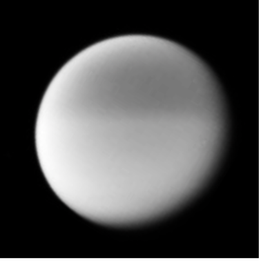
Introduction: Titan’s atmosphere has a north-south haze dichotomy (Fig.1), with an unexpectedly sharp boundary near the equator (e.g., Lorenz et al. 1997; Roos-Serote 2005). The boundary does not sit exactly at the equator, nor does it remain stationary throughout Titan’s year (R. Lorenz 1999; Roman et al. 2009; Kutsop et al. 2022; Vashist et al. 2023; Snell and Banfield 2024). Instead, the boundary migrates in latitude seasonally and is seen to disappear post-equinox then reappear with the dichotomy reversed shortly after. The sharpness of the boundary suggests that there is limited horizontal mixing over the equator. This, in addition to the boundary’s seasonal migration, makes Titan’s equator a dynamically intriguing region. Previously, dynamics in Titan’s stratosphere have been constrained observationally using the thermal wind relation (Sharkey et al. 2021;  Achterberg 2023;  Wright et al. 2025), but this equation breaks down at low latitudes. We instead map infrared-active trace species in Titan’s stratosphere to inspect the dynamics in Titan’s equatorial region.

Data & Method: We use infrared spectra acquired by Cassini’s Composite Infrared Spectrometer (CIRS) instrument from 70 fly-bys of Titan spanning the entire 13-year mission. CIRS had an adjustable spectral resolution, typically observing at FWHM~0.5, 2.5, or 14.5 cm-1. We use CIRS FP3/4 observations acquired at a low spectral resolution (FWHM~14.5 cm-1), which achieved the best combination of seasonal and spatial coverage with high spatial resolution, allowing us to discern compositional variations over finer length-scales than in previous studies (Teanby et al. 2006; Teanby et al. 2010). Wright et al. 2024 showed that these data can be reliably forward-modelled despite having subtle and often blended spectral peaks. We use archNEMESIS (Alday et al. 2025) – an open-source Python package based on the NEMESIS (Irwin et al. 2008) radiative transfer and retrieval code – to fit CIRS FP3/4 spectra. We fit CIRS FP4 spectra by retrieving continuous temperature profiles and fit mid-IR spectra from 600-1100 cm-1 by scaling vertical profiles of gas volume mixing ratio.

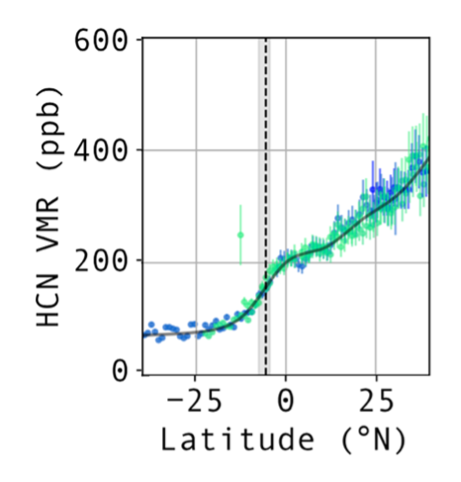
Results: We present maps of the variation in abundances of HCN, C2H2, C2H6, C3H4, C4H2, CO2 in Titan’s stratosphere (~5 mbar pressure) with the highest resolution mapping achieved to date, covering 40oS to 40oN throughout 2004—2017. Many species are seen to have a rapid change in abundance over the equator, with HCN exhibiting the steepest latitudinal gradient (e.g., Fig.2). The improved spatial resolution achieved here allows us to track the migration of the compositional gradient over time. We find that it follows a similar migration to Titan’s north-south haze boundary during the Cassini mission. Haze and HCN distributions appear to behave similarly at the equator, suggesting that the boundary is induced by dynamics, rather than by chemistry or microphysical processes.
In addition, we use the meridional composition gradient to predict the tilt offset of Titan’s stratosphere, following the method of (Teanby et al. 2010). We do this over the full 13-year Cassini mission to inspect the seasonal evolution of Titan’s tilted stratosphere. This is compared to the tilt evolution inferred from temperature (Wright et al. 2025) and from images (Snell and Banfield 2024).


Fig 1. Titan’s north-south albedo asymmetry. Infrared image taken in 2007 by Cassini’s Imaging Science Subsystem (ISS) Narrow-Angled Camera (NAC) using a 890 nm filter.


Fig 2. Retrieved HCN volume mixing ratio (VMR) in Titan’s equatorial region, at 5 mbar. Example from observations taken during 2008. Different colours identify different observation sequences. The steepest gradient is seen to be ~5oS at this time (dashed line, shaded region is the uncertainty).

References

Achterberg, R. K. 2023. The Planetary Science Journal 4 (8): 140. https://doi.org/10.3847/PSJ/acebea.
Alday, J., J. Penn, P. Irwin, J. Mason, J. Yang, and J. Dobinson. 2025. Journal of Open Research Software  13: 10. https://doi.org/10.5334/jors.554.
Irwin, P. G. J., N. A. Teanby, R. de Kok, et al. 2008. Journal of Quantitative Spectroscopy and Radiative Transfer 109 (6): 1136–50. https://doi.org/10.1016/j.jqsrt.2007.11.006.
Kutsop, N. W., A. G. Hayes, P. M. Corlies, et al. 2022. The Planetary Science Journal 3 (5): 114. https://doi.org/10.3847/PSJ/ac582d.
Lorenz, R. 1999. Icarus 142 (2): 391–401. https://doi.org/10.1006/icar.1999.6225.
Lorenz, R. D., P. H. Smith, M. T. Lemmon, E. Karkoschka, G. W. Lockwood, and J. Caldwell. 1997. Icarus 127 (1): 173–89. https://doi.org/10.1006/icar.1997.5687.
Roman, M. T., R. A. West, D. J. Banfield, et al. 2009. Icarus 203 (1): 242–49. https://doi.org/10.1016/j.icarus.2009.04.021.
Roos-Serote, M. 2005. Space Science Reviews 116 (1–2): 201–10. https://doi.org/10.1007/s11214-005-1956-0.
Sharkey, J., N. A. Teanby, Melody Sylvestre, et al. 2021. Icarus 354 (January): 114030. https://doi.org/10.1016/j.icarus.2020.114030.
Snell, C., and D. Banfield. 2024. The Planetary Science Journal 5 (1): 12. https://doi.org/10.3847/PSJ/ad0bec.
Teanby, N. A., P. G. J. Irwin, and R. de Kok. 2010. Planetary and Space Science 58 (5): 792–800. https://doi.org/10.1016/j.pss.2009.12.005.
Teanby, N., P. Irwin, R. Dekok, et al. 2006. Icarus 181 (1): 243–55. https://doi.org/10.1016/j.icarus.2005.11.008.
Vashist, A. S., M. F. Heslar, J. W. Barnes, C. Hennen, and R. D. Lorenz. 2023. The Planetary Science Journal 4 (6): 118. https://doi.org/10.3847/PSJ/acdd05.
Wright, L., N. A. Teanby, P. G. J. Irwin, and C. A. Nixon. 2024. Experimental Astronomy 57 (2): 15. https://doi.org/10.1007/s10686-024-09934-y.
Wright, L, N. A. Teanby, P. G. J. Irwin, et al. 2025. The Planetary Science Journal 6 (5): 114. https://doi.org/10.3847/PSJ/adcab3.

How to cite: Wright, L., Teanby, N. A., Irwin, P. G. J., Nixon, C. A., and Ford, J. S.: High-Resolution Mapping of Titan’s N-S Atmospheric Boundary from Cassini/CIRS, Europlanet Science Congress 2026, The Hague, The Netherlands, 7–11 Sep 2026, EPSC2026-985, https://doi.org/10.5194/epsc2026-985, 2026.

09:36–09:48
|
EPSC2026-968
|
On-site presentation
Zili He, Sandrine Vinatier, Bruno Bézard, Anthony Arfaux, and Pascal Rannou

The spatial distribution of aerosols in Titan’s atmosphere is commonly retrieved from remote-sensing observations of the scattered solar light using one-dimensional plane-parallel or pseudo-spherical radiative transfer solvers. However, such approaches become limited for the analysis of pixels in JWST/NIRSpec observations close to the limb of Titan, because of the large emergent angles that cannot be appropriately treated with the above mentioned solvers. In this work, we present a novel three-dimensional retrieval framework based on the Monte Carlo radiative transfer code htrdr-planets used for the analysis of  JWST/NIRSpec observations of Titan in the near-infrared spectral range acquired in November 2022.

htrdr-planets [1] is a fully spherical and heterogeneous Monte Carlo radiative transfer model developed for planetary atmospheres. This code is modified to simultaneously compute radiances and their sensitivities with respect to atmospheric parameters [2], allowing efficient gradient-based inversions. The present study uses this new radiative transfer solver on NIRSpec observations between approximately 1340 and 1400 nm. This spectral region includes both a methane transmission window and an absorption band, allowing us to probe the aerosol vertical profile at different altitudes from the middle stratosphere to the upper troposphere.

The atmospheric model includes methane absorption treated with the k-distribution method and two aerosol populations: haze above 80 km and mist below 80 km. Aerosol density retrievals are performed using the Jacobians matrix directly estimated by Monte Carlo sensitivity calculations. 

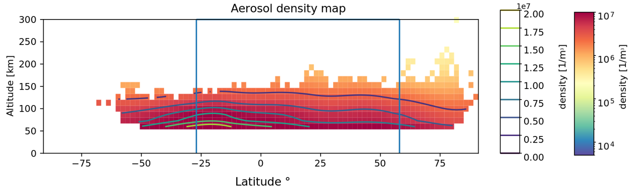
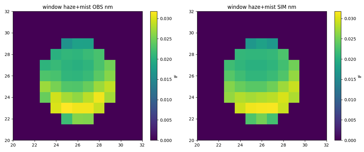
The retrieved aerosol distributions are consistent with previous one-dimensional solver SHDOM-PP inversions of the same observed JWST/NIRSPec pixels close to the center of Titan’s disk [3] (with retrieved information restricted in the 25°S - 60°N region). Here the use of htrdr-planets allows us to analyze a significantly larger number of pixels close to or at the limb thanks to the full 3D treatment of the observation geometry (see Figures 1 and 2). We are then able to extend the probed region to the 60°S - 80°N latitudes range and to the west to east limb. However, we inferred systematic overestimations of the radiance for pixels mixing nadir and limb contributions. 

Figure 1:  JWST/NIRSpec observation of Titan (left) and the htrdr-planets simulation (right) at 1340nm.

Figure 2:  Retrieved aerosol density map using the spherical, heterogeneous Monte Carlo radiative transfer model htrdr-planets, which covers a larger validated area than the aerosol density map retrieved with the classical one-dimensional solver SHDOM-PP (highlighted by the blue frame).


To improve the fit, a multiplicative correction factor on the aerosol scattering albedo is introduced in the inversion procedure. This substantially reduces residuals without strongly modifying the retrieved aerosol density distribution. In addition, introducing longitudinal variations of scattering albedo improves the reproduction of the observed morning–evening asymmetry. This behavior may indicate aerosol condensation processes during Titan’s night side, although additional Monte Carlo realizations are required to confirm this interpretation.

These results demonstrate the capability of three-dimensional Monte Carlo retrieval methods for analyzing JWST/NIRSPec observations and provide new perspectives on studying Titan’s aerosol variability and atmospheric dynamics.

This work has been funded by the French National Research Agency (ANR), project RaD3-net, grant number ANR-21-CE49-0020.


References:
[1] htrdr-planets, https://www.meso-star.com/projects/htrdr/htrdr.html
[2] He, Zili, et al. "Simultaneous Estimation of Radiance and its Sensitivities to Radiative Properties in a Spherical-Heterogeneous Atmospheric Radiative Transfer Model by Monte Carlo: Application to Titan." 2026, JQSRT 350, 109722.
[3] Rannou P. et al., “Mapping Titan’s haze and mist with the near infra-red spectrometer onboard the James Webb space telescope”, 2026, Icarus 450, 116944.

How to cite: He, Z., Vinatier, S., Bézard, B., Arfaux, A., and Rannou, P.: Mapping Titan’s aerosol from JWST/NIRSpec observations with the spherical and heterogeneous Monte Carlo radiative transfer model htrdr-planets, Europlanet Science Congress 2026, The Hague, The Netherlands, 7–11 Sep 2026, EPSC2026-968, https://doi.org/10.5194/epsc2026-968, 2026.

09:48–10:00
|
EPSC2026-448
|
ECP
|
On-site presentation
Anthony Arfaux, Sandrine Vinatier, Pascal Rannou, Vincent Eymet, Vincent Forest, Sébastien Lebonnois, Ehouarn Millour, Bruno de Batz de Trenquelléon, Zili He, and Clément Petetin

Titan’s atmosphere has been extensively studied and modeled over the last twenty years. Global Climate Models (GCMs) successfully reproduce the main features of Titan’s atmosphere, including the detached haze layer and the polar clouds (Lebonnois et al., 2012; Lora et al., 2015; de Batz de Trenquelléon et al., 2025a,b, 2026). However, those models rely on simple plane-parallel radiative transfer algorithms which fail to capture the effects of heterogeneity and sphericity, important for the extended atmosphere of Titan. To address this limitation, we are coupling htrdr-planets (https://www.meso-star.com/projects/htrdr/htrdr.html He et al., 2026), a 3D backward Monte Carlo radiative transfer model, able to account for sphericity and heterogeneity, with the Titan LMDZ Planetary Climate Model (PCM) (de Batz de Trenquelléon et al., 2025a,b, 2026). htrdr-planets incorporates recent developments in computational science (Galtier et al., 2013; Villefranque et al., 2019), and is able to calculate the radiative budget within each PCM cell with minimal approximations and relatively low computational cost.

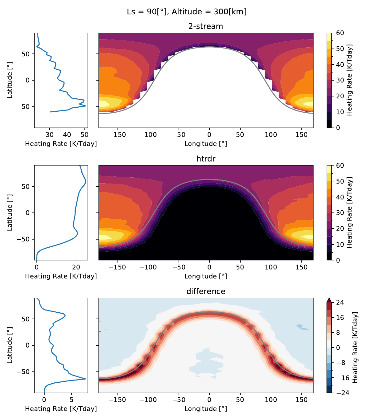
Figure 1: Heating rates at northern summer solstice at 300 km altitude. Upper panels: 2-stream plane-parallel results. Middle panels: htrdr-planets results. Bottom panels: differences htrdr-planets minus plane-parallel. The plots on the left are zonal averages.


Comparisons between the original 2-stream plane-parallel model used in the Titan PCM and htrdr-planets indicates that significant differences are expected at high altitudes in the terminator region (Fig. 1). This behavior is explained by the high incident angles of the stellar radiation near the terminator, which results in larger extinction in a plane-parallel model compared to a spherical scenario. Fig. 1 also demonstrates that, on a zonal average, the main differences are concentrated at the limits of the polar night and polar day, since those regions spend a significant amount of time close to the terminator. In addition, light can directly reach regions beyond the terminator, as a result of sphericity, where plane-parallel calculations cannot be conducted. As a consequence, the spherical model produces additional heating in the regions beyond the terminator in the spherical model relatively to the plane-parallel.

To explore how the observed heterogeneity and sphericity effects impact the thermal structure and dynamic of Titan’s atmosphere, we couple htrdr-planets to the Titan PCM. This is realized by running htrdr-planets every 11 Titan days, with optical properties extracted from the Titan PCM. The calculated heating rates are then used in the Titan PCM with an interpolation in solar longitude and local time. For the sake of computation time, we focus our efforts on the solar  heating and keep the original 2-stream model to calculate the thermal cooling.


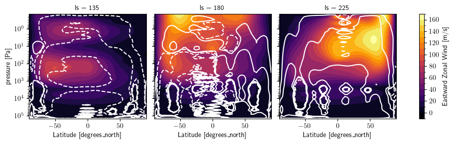
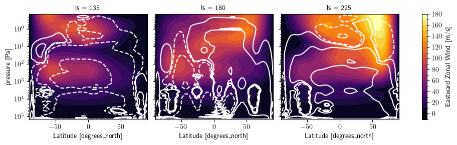
Figure 2: Wind maps around the northern fall equinox. The color scale presents the zonal winds, white lines represent the streamfunction, where dashed lines indicate counter-clockwise circulation and solid lines indicate clockwise circulation. Upper panels: reference PCM calculation. Bottom panels: PCM simualtion coupled to htrdr-planets. Panels on the left are at LS = 135° , middle panels are at LS = 180° and right panels are at LS = 225° .


Preliminary results of this coupling demonstrate that the changes brought by the modified heating rates on the dynamics of Titan’s atmosphere are important. We observe changes in the stability of the Hadley cell as well as modifications in the timing of appearance of this structure (Fig. 2). In addition, smaller yet stable cells appear in the upper stratosphere and are expected to affect the transport of various species, as well as haze particles. Such changes have major ramifications for the thermal structure of the atmosphere.

In this presentation, we detail those initial comparisons between htrdr-planets and a 2-stream plane-parallel model and we explore the preliminary results of the coupling between htrdr-planets and the Titan PCM.


This work has been funded by the French National Research Agency (ANR), project RaD3-net, grant number ANR-21-CE49-0020.


References
de Batz de Trenquelléon, B., et al. (2025a). The New Titan Planetary Climate Model. II. Titan’s Haze and Cloud Cycles. The Planetary Science Journal, 6, 79.
de Batz de Trenquelléon, B., et al. (2026). Origin, evolution, and fate of Titan’s polar clouds. Nature Communications, 17 , 250.
de Batz de Trenquelléon, B., et al. (2025b). The New Titan Planetary Climate Model. I. Seasonal Variations of the Thermal Structure and Circulation in the Stratosphere. The Planetary Science Journal, 6, 78.
Galtier, M., et al. (2013). Integral formulation of null-collision Monte Carlo algorithms. Journal of Quantitative Spectroscopy and Radiative Transfer, 125, 57–68.
He, Z., et al. (2026). Simultaneous estimation of radiance and its sensitivities to radiative properties in  a spherical-heterogeneous atmospheric radiative transfer model by Monte Carlo method: Application to Titan. Journal of Quantitative Spectroscopy and Radiative Transfer, 350, 109722.
Lebonnois, S., et al. (2012). Titan global climate model: A new 3-dimensional version of the IPSL Titan GCM. Icarus, 218(1), 707–722.
Lora, J. M., et al. (2015). GCM simulations of Titan’s middle and lower atmosphere and comparison to observations. Icarus, 250, 516–528.
Villefranque, N., et al. (2019). A Path-Tracing Monte Carlo Library for 3-D Radiative Transfer in Highly Resolved Cloudy Atmospheres. Journal of Advances in Modeling Earth Systems, 11(8), 2449–2473.

How to cite: Arfaux, A., Vinatier, S., Rannou, P., Eymet, V., Forest, V., Lebonnois, S., Millour, E., de Batz de Trenquelléon, B., He, Z., and Petetin, C.: htrdr-planets & Titan PCM: coupling Monte Carlo radiative transfer and Planetary Climate Models, Europlanet Science Congress 2026, The Hague, The Netherlands, 7–11 Sep 2026, EPSC2026-448, https://doi.org/10.5194/epsc2026-448, 2026.

Orals FRI2: Fri, 11 Sep, 11:00–12:30 | Room Jupiter (Jazz 1 & 2)

Chairpersons: Bruno de Batz de Trenquelléon, Robin Sultana
11:00–11:03
Modelling the methane cycle
11:03–11:15
|
EPSC2026-114
|
ECP
|
On-site presentation
Lucie Rosset, Audrey Chatain, Clément Petetin, Enora Moisan, Bruno de Batz de Trenquelléon, Yassin Jaziri, and Nathalie Carrasco

1. Introduction

Titan, Saturn’s biggest moon, has a thick atmosphere composed mainly of nitrogen and methane. Atmospheric conditions allow methane to be present in solid, liquid, and gaseous state. As a result, Titan has a methane cycle similar to Earth’s water cycle, featuring clouds, precipitation, and lakes and seas on the surface [1]. In addition to convective methane clouds forming in the troposphere, hydrocarbon clouds at the poles and high-altitude HCN clouds have also been observed [2,3]. Nevertheless, observations of Titan’s clouds remain limited, and questions persist regarding the distribution and composition of the clouds [4]. In this context, numerical climate models allow for a better understanding of the various mechanisms at work, as well as a deeper understanding of the observations. This presentation will discuss the atmospheric distribution of methane and its impact on cloud formation and evolution, as well as the impact on Titan’s climate.

2. Methane condensation and  clouds in the troposphere

To tackle these questions, we use the Titan Planetary Climate Model (Titan LMDZ PCM [5]), a 3D climate model that simulates Titan’s climate at a global scale. It includes a fully coupled microphysical model in moments for haze and clouds [6]. The model takes into account the nucleation, condensation, sedimention and precipitation of six species : CH4, C2H2, C2H6, HCN, HC3N and AC6H6 [7]. Currently, the model condensates these species as ices only, and independently of each other, however some methane clouds are also likely to be formed of liquid droplets [8].

The abundance of methane in the model was previously constrained by Huygens measurements, with a minimum concentration set at 1.4%. Recent reanalysis of CIRS observations show that the Huygens measurements were atypical and that the concentration of methane in the stratosphere is generally lower, around ~1%, varying seasonally by +/-0.4% [9]. We therefore decided to remove this minimum value from the model and allow methane to evolve freely. 

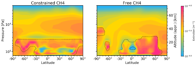
We find that this affects the altitude of saturation of methane and thus cloud formation in the model. Preliminary results show that the vertical and seasonal distribution of methane clouds is improved. The top altitude of methane clouds is allowed to increase. Methane clouds form in a more localised manner in the low and mid-latitudes of the summer hemisphere, which is more coherent with the observations (Fig 1).


Figure 1 : Comparison between the zonally averaged cloud extinction at 0.7µm during northern summer (Ls=135°) for simulation with and without constrained methane. Methane ice presence is indicated by the black contour.

3. Methane concentration in the stratosphere

The concentration of stratospheric methane reaches 0.7% after 30 years of simulation (Fig 2). Although consistent with the lower limit of observations, these values correspond to isolated events and vary with latitude and season (see abstract by Olwen Rering). We conclude that the model lacks a mechanism that would replenish methane in the stratosphere. 


Figure 2 : Modeled methane profiles at the region and period of Huygens compared to Huygens measurements.

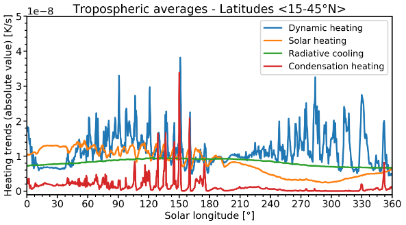
We are currently adding to the model the latent heat release due to the condensation of condensible species. This is the main mechanism underlying the development of methane storms, that are thought to allow methane to be transported to higher altitudes [10]. Preliminary results show that the energy contribution from condensation in the troposphere, at the latitudes and periods of modeled cloud activity, is significant (Fig 3). 


Figure 3 : Comparison between the energetic contribution (in absolute value) of the global circulation (blue), the solar heating (orange), the radiatively active species (green) and the computed contribution of condensation (red). Values are averaged from the surface to 2.10⁴ Pa for latitudes between 15 and 45°N.

References

[1] Turtle et al. « Titan’s Meteorology Over the Cassini Mission: Evidence for Extensive Subsurface Methane Reservoirs ». Geophysical Research Letters 45, no 11 (2018): 5320‑28. https://doi.org/10.1029/2018GL078170.

[2] West et al. « Cassini Imaging Science Subsystem observations of Titan’s south polar cloud ». Icarus, 270  (2016) , 399-408. https://doi.org/10.1016/j.icarus.2014.11.038 

[3] de Kok et al., « HCN Ice in Titan’s High-Altitude Southern Polar Cloud », Nature 514, no 7520 (2014): 7520, https://doi.org/10.1038/nature13789.

[4] Nixon, Carrasco, Sotin, « Chapter 15 - Open questions and future directions in Titan science», In COSPAR Series, Titan After Cassini-Huygens, Elsevier (2025), Pages 473-515, ISBN 9780323991612, https://doi.org/10.1016/B978-0-323-99161-2.00012-7. 

[5] de Batz De Trenquelléon et al. « The New Titan Planetary Climate Model. I. Seasonal Variations of the Thermal Structure and Circulation in the Stratosphere ». The Planetary Science Journal 6, no 4 (2025): 78. https://doi.org/10.3847/PSJ/adbbe7.

[6] de Batz De Trenquelléon et al. « The New Titan Planetary Climate Model. II. Titan’s Haze and Cloud Cycles ». The Planetary Science Journal 6, no 4 (2025): 79. https://doi.org/10.3847/PSJ/adbb6c .

[7] de Batz De Trenquelléon et al., « Origin, Evolution, and Fate of Titan’s Polar Clouds », Nature Communications, (2025), https://doi.org/10.1038/s41467-025-66955-7. 

[8] Wang et al., « Methane gas stabilizes supercooled ethane droplets in Titan’s clouds », The Astrophysical Journal 712, no 1 (2010): 1, https://doi.org/10.1088/2041-8205/712/1/L40.

[9] Lellouch et al., « The Distribution of Methane in Titan’s Stratosphere from Cassini/CIRS Observations », Icarus 231 (2014): 323‑37, https://doi.org/10.1016/j.icarus.2013.12.016.

[10] Moisan et al., « Modeling Convective Methane Clouds on Titan with a Kilometer-Scale Regional Model », abstract. presented at EGU (2026) https://doi.org/10.5194/egusphere-egu26-13288.

How to cite: Rosset, L., Chatain, A., Petetin, C., Moisan, E., de Batz de Trenquelléon, B., Jaziri, Y., and Carrasco, N.: Methane cloud formation and impact on the climate of Titan with the Titan LMDZ PCM , Europlanet Science Congress 2026, The Hague, The Netherlands, 7–11 Sep 2026, EPSC2026-114, https://doi.org/10.5194/epsc2026-114, 2026.

11:15–11:30
|
EPSC2026-543
|
ECP
|
On-site presentation
Enora Moisan, Audrey Chatain, and Aymeric Spiga

Context: Titan's methanologic cycle

Titan's methane cycle is very similar to Earth's hydrologic cycle: evaporation from liquid bodies at the surface, condensation and cloud formation in the troposphere, rain (Hayes et al. 2018). Here, we focus on the clouds' formation and evolution.

Methods:

We use the Titan WRF PCM model: a regional model based on the coupling of the Weather Research and Forecast (WRF) dynamical core with the physics of the Titan Planetary Climate Model (Titan PCM, Lebonnois et al. 2012, de Batz de Trenquelléon et al. 2025a, de Batz de Trenquelléon et al. 2025b).

We use it in 3D, with a domain of 60x60km and a horizontal resolution of 1km. The top of the model is around the tropopause, at 50km, and the vertical resolution goes from 3m close to the surface to 1.8km at the model top. Our time step is of 0.5s. We set our simulation at a latitude and season where we expect convective clouds to appear: during the southern summer, close to the south pole. Indeed, clouds are predicted there by general circulation models (de Batz de Trenquelléon et al. 2025b), and were observed in 2004 by Cassini (Porco et al. 2005). The simulation is initialized with profiles from the general circulation model (Titan LMDZ PCM), for temperature, methane vapor, and aerosols. We trigger convection with a warm bubble at the center of the domain, 1K warmer than the environment, and we let the situation evolve. The warm bubble is an ellipsoid with horizontal semi-axes of 5km and a vertical semi-axis of 500m, laying on the surface.

Modeled cloud

Figure 1 shows the evolution of the cloud.

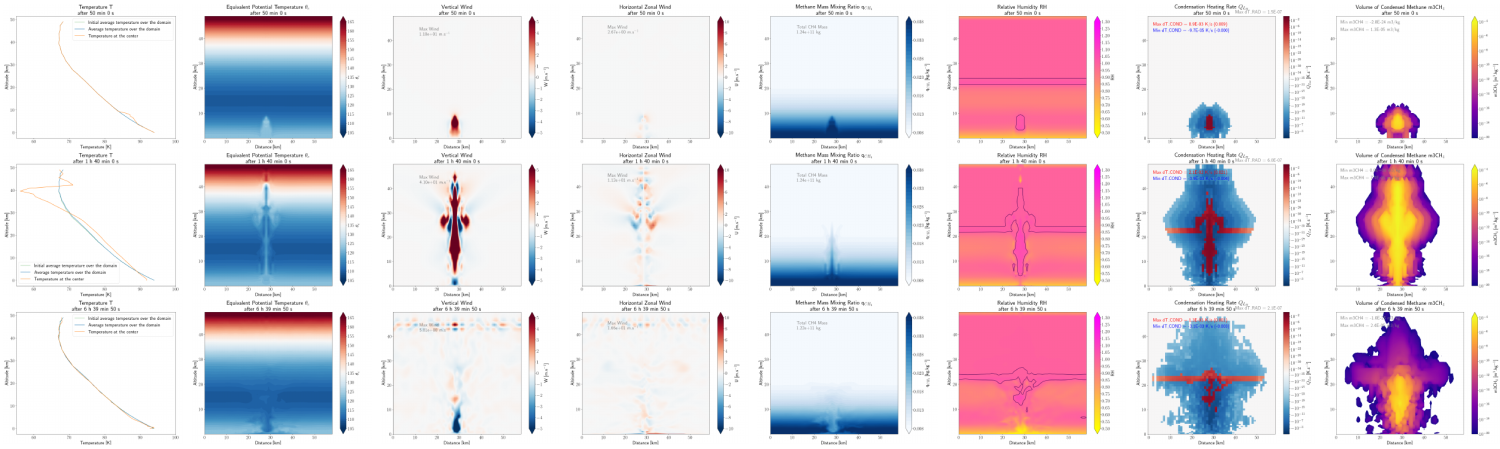
Figure 1: Evolution of the simulation (temperature, equivalent potential temperature, vertical wind, horizontal wind, methane vapor, relative humidity, condensation heating rate, volume of condensed methane). First line: 50min after run start, Second line: 1h40 after run start, Third line: 6h39 after run start.

The warm bubble has a positive buoyancy (see the temperature profiles and the equivalent potential temperature figures, columns 1 and 2). As a result, it rises in the atmosphere, transporting methane upward (see the vertical wind (column 3) and the evolution of the methane vapor (column 5)). As the temperature decreases in altitude the air reaches a point of saturation, causing methane condensation (see the relative humidity (column 6) and the condensation heating rate (column 7)). Once the condensation is triggered, it releases latent heat (positive condensation heating rate), which increases the temperature and the buoyancy, causing the air to continue its motion upward: the cloud is convective.

Column 8 shows the volume of condensed methane, i.e. the volume of cloud at each point. The cloud forms ~35min after the start of the simulation (~5km above the surface), and then extends upward (updraft) and downward (precipitations and unsaturated downdrafts) during ~1h. The updrafts and downdrafts are visible in the vertical wind column (column 3). When the unsaturated downdrafts reach the surface they spread horizontally, forming cold pools. The maximum horizontal wind at the surface is ~24m.s-1 (in the first level, i.e. ~3m above the surface). The cloud reaches the top of the model ~1h20 after the start of the simulation. Afterwards, it extends horizontally, during ~1h30, and the cloud top lowers slowly. The cloud's maximal horizontal extent is ~50km.

The storm produces in total 0.03kg.m-2 of precipitations (corresponding to 0.011mm.h-1 of rain on average over the domain and a total of 0.076mm during the simulation). Taking only the parts of the domain receiving rain, the precipitations are of ~0.033mm.h-1 on average (i.e. 0.22mm in total, or 0.09kg.m-2). At the peak it rains 9.5mm in 1min, corresponding to a precipitation rate of 569mm.h-1; the maximum hourly cumulative rainfall is 159mm. For a rough estimate, we can say that precipitations during the storm are on average in the range 0.01-0.1mm.h-1, and around 100mm.h-1 at the storm maximum. In comparison, storm Ciarán (which hit the Channel Island and the North of France in November 2024) produced a maximum rain rate of 175mm.h-1 over one minute (Winter et al. 2024), while the world record rainfall is 300mm in 42min (Lott 1954).

Other simulations

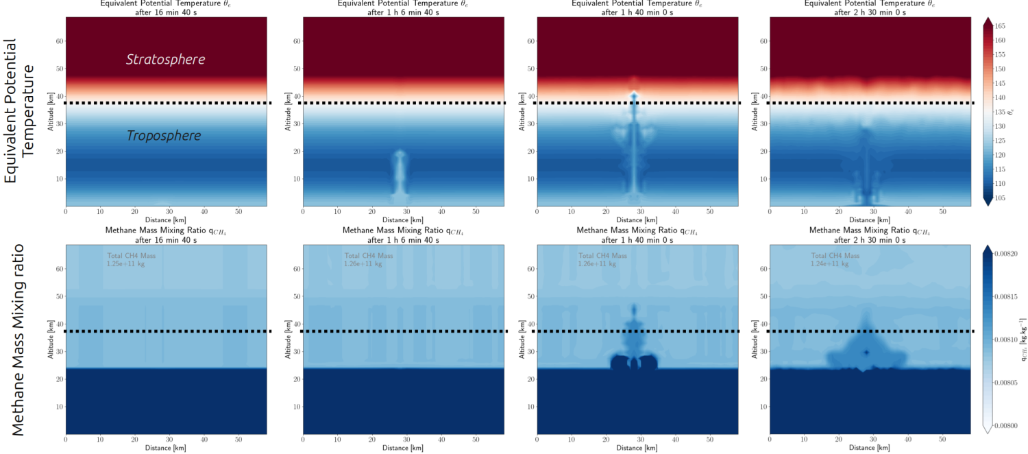
To study the altitude the cloud would reach without the artificial barrier of the model top, we perform a run with a top at 70km. We obtain a maximal cloud top around 60km. This simulation also enables us to see that the modeled convective cloud introduces some methane vapor in the stratosphere (see Figure 2). This phenomenon could explain the observed stratospheric methane variability, as suggested by Rannou et al. 2021.

Moreover, by changing the season we are able to reproduce some seasonal variability of the methane convective clouds (i.e. bigger clouds at the south pole than at the equator during the southern summer).

Figure 2: First Row: Equivalent potential temperature. Second Row: Methane vapor. Columns: time after run start (16min 40s, 1h 6min 40s, 1h 40min 0s, 2h 30min 0s). The dashed line indicates the tropopause.

Rerefences

de Batz de Trenquelléon et al. 2025a “The New Titan Planetary Climate Model. I. Seasonal Variations of the Thermal Structure and Circulation in the Stratosphere”. (The Planetary Science Journal)

de Batz de Trenquelléon et al. 2025b “The New Titan Planetary Climate Model. II. Titan’s Haze and Cloud Cycles”. (The Planetary Science Journal)

Hayes et al. 2018. “A Post-Cassini View of Titan’s Methane-Based Hydrologic Cycle”. (Nature Geoscience)

Lebonnois et al. 2012. “Titan Global Climate Model: A New 3-Dimensional Version of the IPSL Titan GCM”. (Icarus)

Lonfat et al. 2004. “Precipitation Distribution in Tropical Cyclones Using the Tropical Rainfall Measuring Mission (TRMM) Microwave Imager: A Global Perspective”. (Monthly Weather Review)

Lott, G.A., 1954. "The World Record 42-minute Holt, Missouri, Rainstorm". Monthly Weather Review

Porco et al. 2005. “Imaging of Titan from the Cassini Spacecraft”. (Nature)

Rannou et al. 2021. “Convection behind the Humidification of Titan’s Stratosphere”. (The Astrophysical Journal)

Winter et al. 2024. “Storm Ciarán – an Exceptionally Severe Windstorm in the Channel Islands”. (Weather)

How to cite: Moisan, E., Chatain, A., and Spiga, A.: Modeling convective methane clouds on Titan with a regional model, Europlanet Science Congress 2026, The Hague, The Netherlands, 7–11 Sep 2026, EPSC2026-543, https://doi.org/10.5194/epsc2026-543, 2026.

11:30–11:42
|
EPSC2026-517
|
ECP
|
On-site presentation
Clément Petetin, Pascal Rannou, Sébastien Lebonnois, Bruno De Batz de Trenquelléon, and Lucie Rosset

1 Introduction
In Titan’s atmosphere and on its surface, methane plays a crucial role in the global climate. Since the methane cycle resembles Earth’s water cycle, with many similar processes as evaporation, condensation, rains and On Titan, condensed methane forms clouds and bodies of liquid at the surface (lakes, seas). One important aspect of Earth’s water cycle is infiltration into the ground, storage, and large scale transport in underground aquifers. On Titan, similar process should be at work too ([1], [2]). We already know that methane precipitation occurs on Titan’s surface and infiltration [3], and that the surface is moist [4]. We then assume that methane can infiltrates Titan’s soil, creating a subsurface cycle that participates to the surface/atmosphere exchanges and to planetary scale horizontal flux. In addition, it could also change locally the soil’s properties and its temperature. The underground aspects of the methane cycle are not well understood, and models struggle to reproduce some keys observation as, for instance, the cloud cycle. However implementing a representation of the subsurface methane cycle and its effect on the atmosphere and on the surface will help to constrain some unknow parameters of the underground of Titan.

2 Objective and method
The Titan Planetary Climate Model, first developed at the Institut Pierre-Simon Laplace ([5],[6]), is a useful and powerful tool for exploring Titan’s climate, especially the methane cycle. The Titan PCM employs an advanced microphysical scheme. [7] to simulate the complex cloud physics within Titan’s troposphere. This scheme enables a realistic representation of the methane cycle through condensation, evaporation, and precipitation processes in the lower layers of the atmosphere. However, exchanges between atmospheric and surface methane are still treated in a simplified manner (Figure 1). The goal of this work is to develop and use a comprehensive model that better captures the interactions between the surface, the subsurface, and the atmosphere.
For the inclusion of a subsurface model in Titan’s PCM, we use a quasi-3D model that computes the vertical flux of liquid in a one dimensional column and the horizontal transport in a two dimensional diffusion scheme using hydrodynamics equations. This follow the same general principle than behind the model described in [1] although our infiltration model for vertical flux differs and will be explained. In addition, Titan is known to host different types of terrain. These variations play a fundamental role in the soil’s ability to retain liquid within its pores. Characterizing and parameterizing these terrains in a realistc way is therefore a key challenge in implementing our subsurface model. The soil’s porosity and drainage capacity must be set to values representative of sandy loam, a soil type expected from the accumulation and compaction of tholins at Titan’s surface.


3 Results
In our presentation, we will discuss the main properties and performances of the surface model that we have developed and the way it is implemented in the Titan PCM. Then in a second place, we will show the main outcomes of the reference model, without subsurface processes, and the new model that includes the full subsurface model. One of the most important parameter of the model is the permeability of the soil. because it controls the retention
time of the liquid methane. Other parameters may also alter the final results such as the porosity or the methane table depth. We will then discuss the effect of these different key parameters on the modeled methane cycle.
For this discussion, we will essentially focus on the differences in the spatial distribution of gaseous methane and methane cloud, precipitations and methane flux at planetary scale in the atmosphere and in the subsurface. Several scenarios will be considered and our model will be compared to others availables simulations ([7],[1]).


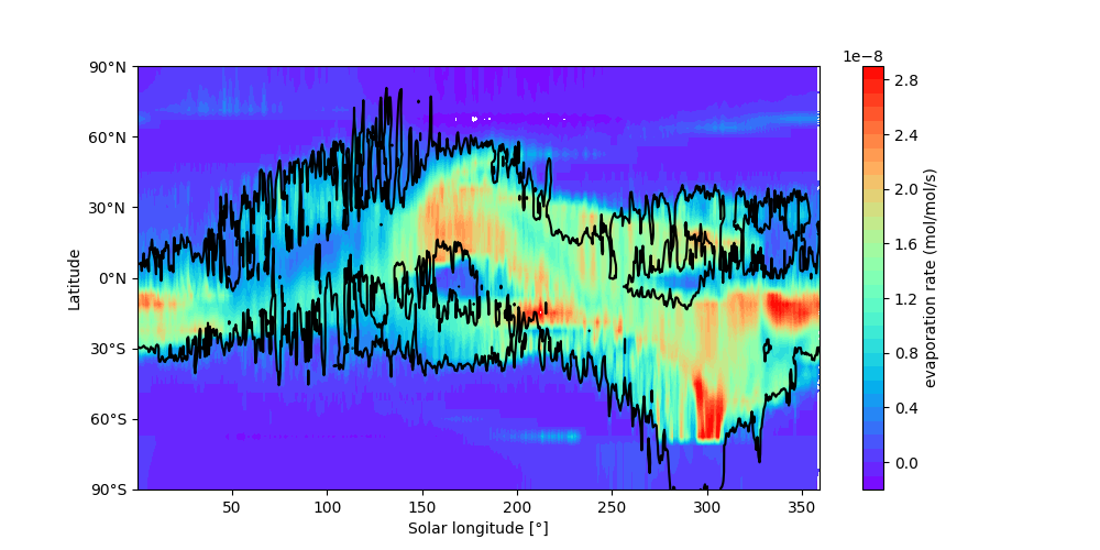
Figure 1: Seasonal evolution of the simple case of the methane flux scheme simulated by the Titan PCM before the
subsurface model. The map displays the evaporation rate, while the black contours indicate the spatial distribution
of methane precipitation over one Titan year.


References
[1] Sean P. Faulk, Juan M. Lora, Jonathan L. Mitchell, and P. C. D. Milly. Titan’s climate patterns and surface methane distribution due to the coupling of land hydrology and atmosphere. Nature Astronomy, 4:390–398, January 2020.
[2] Tetsuya Tokano. Stable existence of tropical endorheic lakes on titan. Geophysical Research Letters, 47(5):e2019GL086166, 2020. e2019GL086166 10.1029/2019GL086166.
[3] E. P. Turtle, J. E. Perry, J. M. Barbara, A. D. Del Genio, S. Rodriguez, S. Le Mouélic, C. Sotin, J. M. Lora, S. Faulk, P. Corlies, J. Kelland, S. M. MacKenzie, R. A. West, A. S. McEwen, J. I. Lunine, J. Pitesky, T. L. Ray, and M. Roy. Titan’s Meteorology Over the Cassini Mission: Evidence for Extensive Subsurface Methane Reservoirs. , 45(11):5320–5328, June 2018.
[4] H. B. Niemann, S. K. Atreya, S. J. Bauer, G. R. Carignan, J. E. Demick, R. L. Frost, D. Gautier, J. A. Haberman, D. N. Harpold, D. M. Hunten, G. Israel, J. I. Lunine, W. T. Kasprzak, T. C. Owen, M. Paulkovich, F. Raulin, E. Raaen, and S. H. Way. The abundances of constituents of Titan’s atmosphere from the GCMS instrument on the Huygens probe. , 438(7069):779–784, December 2005.
[5] Sébastien Lebonnois, Jérémie Burgalat, Pascal Rannou, and Benjamin Charnay. Titan global climate model: A new 3-dimensional version of the IPSL Titan GCM. , 218(1):707–722, March 2012.
[6] Bruno de Batz de Trenquelléon, Lucie Rosset, Jan Vatant d’Ollone, Sébastien Lebonnois, Pascal Rannou, Jérémie Burgalat, and Sandrine Vinatier. The new titan planetary climate model. i. seasonal variations of the thermal structure and circulation in the stratosphere. The Planetary Science Journal, 6(4):78, mar 2025.
[7] Bruno de Batz de Trenquelléon, Pascal Rannou, Jérémie Burgalat, Sébastien Lebonnois, and Jan Vatant d’Ollone. The new titan planetary climate model. ii. titan’s haze and cloud cycles. The Planetary Science Journal, 6(4):79, mar 2025.

How to cite: Petetin, C., Rannou, P., Lebonnois, S., De Batz de Trenquelléon, B., and Rosset, L.: Effect of subsurface on the methane cycle in Titan's atmosphere with a Planetary Climate Model, Europlanet Science Congress 2026, The Hague, The Netherlands, 7–11 Sep 2026, EPSC2026-517, https://doi.org/10.5194/epsc2026-517, 2026.

Irradiation and charging in the atmosphere
11:42–11:54
|
EPSC2026-430
|
On-site presentation
Antoine Damiens and Panayotis Lavvas

In Titan’s atmosphere, haze formation is initiated in the upper atmosphere (~900-1200 km) through photodissociation of N2 and CH4 , producing radicals, ions, and increasing complexity molecules [1, 2]. These chemical processes give rise to an upper ionosphere whose structure and composition have been revealed by the Cassini mission that subsequently performed in situ measurements of this upper ionosphere down to 950 km altitude. Mass spectra and charge distribution measurements revealed complex molecules up to ~100 amu with the Ion and Neutral Mass Spectrometer (INMS), and a plasma of heavy positively and negatively charged molecules up to 350-1000 amu with the Cassini Plasma Spectrometer Ion Beam Spectrometer (CAPS-IBS) [1, 3]. These heavy ions were shown to be directly linked to the photochemical haze formation mechanism at ~1000 km [4]. Magnetospheric ions have also been shown to contribute to a fraction of upper ionosphere ionization [5, 6, 4], espacially during nightside [7]. Aerosols embedded in an ionosphere acquire preferentially negative charges due to the higher mobility of electrons relative to positive ions, thereby depleting the electron population. Below 1000 km, the ionosphere behaves as a dusty plasma [4], and ions become the dominant mobile charge carriers, as the negatively charged dust grains are comparatively heavier. Aerosol growth in the ionosphere occurs primarily through collisions between negatively charged haze particles and positive ions, and their electric charge governs their coagulation efficiency, and coupling to the ionospherere. 

In 2005, the Huygens probe obtained in situ measurements of conductivity during its descent using the Mutual Impedance (MI) and Relaxation Probe (RP) sensors [8, 9], revealing a second ionospheric layer near 65 km [10, 11] where the electron density peaks [12]. Unlike the upper ionosphere, this layer is almost independent of the solar cycle, as ionization is driven by the most energetic galactic cosmic rays (GCRs) particles capable of penetrating to such depths [13, 14, 15, 16]. GCRs ionize neutral constituents, producing positive ions and electrons. MI and RP sensors data indicate peak charge densities of positive ions and electrons between 60 and 70 km [8, 9]. 

The conductivity of the lower atmosphere is a topic of investigation for reproducing Huygens measurements [17]. Recent studies [12] find that the inclusion of aerosol particles reduces charge concentrations, with the reduction being more pronounced for electrons, and deduced that the electron trapping in aerosols leads a charge per radius of ≈ 60 charges/µm. 

Here we use a self consistent model of photochemistry, microphysics and radiative transfer to investigate charge distribution across a full atmopsheric column. The model was originally developed by [18, 19, 20] and previously applied to the study of the upper ionosphere [21, 4]. We adapted its latest version, used by [22] to study the southern polar region during the post-equinox period. In Titan’s atmosphere, haze particles acquire charge through two competing mechanisms : (i) photoelectric emission driven by the solar UV flux, and (ii) collisional capture of ions and electrons from the gas phase. To compute those rates, we follow [23] for the photoelectric yield and electron sticking efficiency, and [24] for the collisional charging rates. Electron and ion density profiles, along with charged particles connect the upper and lower ionosphere. We will discuss the resulting particle charge distributions and compare with available observations through out the atmosphere. Moreover, we will evaluate the feedback between the gas and particulate phases through the involved heterogeneous processes.

[1] J. H. Waite et al., Science, vol. 316, pp. 870–875 (2007).
[2] V. Vuitton et al., Icarus, vol. 324, pp. 120–197 (2019).
[3] A. Coates et al., Planet. Space Sci., vol. 57, pp. 1866–1871 (2009).
[4] P. Lavvas et al., Proc. Natl. Acad. Sci., vol. 110, pp. 2729–2734 (2013).
[5] T. E. Cravens et al., Geophys. Res. Lett., vol. 35, p. 2007GL032451 (2008).
[6] E. C. Sittler et al., In : Titan from Cassini-Huygens, pp. 393–453 (2009).
[7] J. H. Westlake et al., J. Geophys. Res. Space Phys., vol. 119, pp. 5951–5963 (2014).
[8] M. Hamelin et al., Planet. Space Sci., vol. 55, pp. 1964–1977 (2007).
[9] J. J. López-Moreno et al., Geophys. Res. Lett., vol. 35, p. 2008GL035338 (2008).
[10] M. Fulchignoni et al., Nature, vol. 438, pp. 785–791 (2005).
[11] R. Grard et al., Planet. Space Sci., vol. 54, pp. 1124–1136 (2006).
[12] G. Molina-Cuberos et al., Planet. Space Sci., vol. 153, pp. 157–162 (2018).
[13] L. A. Capone et al., Icarus, vol. 55, pp. 73–82 (1983).
[14] G. Molina-Cuberos et al., Planet. Space Sci., vol. 47, pp. 1347–1354 (1999).
[15] G. Gronoff et al., Astron. Astrophys., vol. 506, pp. 955–964 (2009).
[16] G. Gronoff et al., Astron. Astrophys., vol. 529, p. A143 (2011).
[17] R. D. Lorenz, Icarus, vol. 354, p. 114092 (2021).
[18] P. Lavvas et al., Planet. Space Sci., vol. 56, pp. 67–99 (2008).
[19] P. Lavvas et al., Planet. Space Sci., vol. 56, pp. 27–66 (2008).
[20] P. Lavvas et al., Icarus, vol. 215, pp. 732–750 (2011).
[21] P. Lavvas et al., Icarus, vol. 213, pp. 233–251 (2011).
[22] A. Damiens and P. Lavvas, EPSC-DPS Joint Meeting 2025, EPSC-DPS2025-279 (2025).
[23] J. C. Weingartner and B. T. Draine, Astrophys. J. Suppl., vol. 134, pp. 263–281 (2001).
[24] B. T. Draine and B. Sutin, Astrophys. J., vol. 320, p. 803 (1987).

How to cite: Damiens, A. and Lavvas, P.: Unraveling the connection of charge distribution in Titan’s upper and lower ionosphere, Europlanet Science Congress 2026, The Hague, The Netherlands, 7–11 Sep 2026, EPSC2026-430, https://doi.org/10.5194/epsc2026-430, 2026.

11:54–12:06
|
EPSC2026-508
|
ECP
|
On-site presentation
Elsa Hénault, Véronique Vuitton, Eric Quirico, Filip Matuszewski, Zoltán Juhász, Richárd Rácz, Sándor Biri, Gergő Lakatos, Nandalal Mahapatra, Robert W. McCullough, Thomas A. Field, Nigel J. Mason, Alicja Domaracka, Hermann Rothard, David Dubois, Thibault Nguyen Trung, Sreeja Raghunandanan, Simon Ollivier, and Carlos Afonso

The Cassini-Huygens mission revealed great complexity in Titan’s atmosphere. Indeed, mass spectrometers onboard Cassini detected the presence of ions of unexpectedly high masses [1]. These macromolecular ions are understood as the precursors of the aerosols abundant at lower altitude with formation mechanisms likely driven by ion chemistry [2]. These precursor molecules probably are polycyclic aromatic (nitrogen bearing) hydrocarbons (PAHs & N-PAHs) identified by their C-H infrared emission signatures [3], compatible with the detected ion mass-to-charge ratios [4]. Chemistry in ionospheres is triggered by UV photons and energetic particles pervading the Solar System. But specific to Titan is its place within Saturn’s magnetosphere where oxygenated ions, sourced from the plumes of Enceladus, were detected. 10 to 100 keV oxygen ions can reach fluxes of ~106 ions.cm-2.s-1 in Titan’s upper atmosphere [5]. Ions typically deposit on Titan between 1200 and 800 km in altitude and mainly loose energy until thermalization by interactions with N2 [6]. Yet a fraction of these ions must interact directly with the organics and contribute to Titan’s complex chemistry. As ion irradiation is known to trigger sputtering, chemical growth and possibly implantation, what is the impact of these processes on Titan’s chemical budget?

Titan’s atmospheric chemistry has been historically investigated by subjecting N2:CH4 mixtures to representative energy sources triggering photolysis and radiolysis [7]. The resulting aerosol analogs, called “tholins”, are made of irregular polymeric structures with unsaturation levels indicative of N-PAHs, with infrared features of amines, (iso)cyanides, aliphatic and heteroaromatic groups. Tholins exposed to VUV [8] and plasma [9] irradiation showed erosion on the grains and non-uniform modification of chemical functions. Here, we used N-PAHs as simpler aerosol analogues to investigate and quantify distinct and competing processes triggered by ion irradiation. High resolution mass spectrometry analysis of O+-irradiated adenine (C5H5N5) showed the formation of different families of (HCN)-like polymeric structures of condensed aromatics [10]. During irradiation, sputtering also occurs and expels small molecules to the gas phase, typically HCN, comparable to plasma-driven erosion [11]. But adenine is not fully representative of Titan aerosols as tholins show a range of N/C ratios from 1.5 to 0 [12]. To get a broader picture of oxygen irradiation on a range of representative molecules, we have conducted new experiments on adenine, adenine:chrysene mixtures, bathophenanthroline (C24H16N2) and chrysene (C18H12) with N/C ratios of 1, ~0.2, 0.08 and 0 respectively.

Irradiation experiments were performed at the ARIBE beam line coupled to the IGLIAS chamber at GANIL (Caen, France) [13] and at the HUN-REN Institute for Nuclear research (Atomki) in Debrecen (Hungary) with the AQUILA chamber [14] and the Electron Cyclotron Resonance ion source [15]. We used oxygen ions at 10 and 20 keV (for 18O) and at 70 and 108 keV (for 16O) to irradiate samples at 150 or 300 K with maximum fluences of 2x10¹⁶ ions/cm2. The experimental rationale varied depending on the process we aimed to quantify: single layers of hundreds of nanometers for sputtering and multiple layers for implantation. In-situ infrared spectroscopy and quadrupole mass spectrometry measurements are performed to track chemical changes and sputtering.

Infrared analysis shows the progressive destruction of the initial molecular film, associated to its intact sputtering and to radiolysis followed by sublimation of volatile species [16]. The appearance of new bands allows to identify and quantify abundant radiolytic products, associated with dehydrogenation processes. Samples irradiated with 18O ions were analyzed ex-situ with an 18T-FT-ICR mass spectrometer at the CARMeN Institute (Rouen, France) with a resolution allowing unambiguous detection of implanted 18O. The molecular content of the irradiated samples was analyzed by Laser Desorption Ionization, revealing high molecular complexity with m/z reaching 700.

We will present experimental results that provide insights into the heterogeneous processes in Titan’s upper atmosphere. By extracting sputtering yields and destruction cross sections, we provide input for photochemical-microphysical models of Titan’s complex atmosphere. By probing molecular growth through oxygen incorporation into C,H,N material, we investigate an added prebiotic interest for the aerosols sedimenting to the surface. This work can also have implications for outer solar system bodies like Triton, Pluto, Eris and Makemake where oxygen ions of the solar wind and galactic cosmic rays process ices and transient atmospheres of high hydrocarbon content.

Acknowledgments

This work is supported by the French National Research Agency in the framework of the "Investissements d’avenir” program (ANR-15-IDEX-02) and the generic call for proposals (ANR-22-CE49-0017). The experiments were performed at the Grand Accélérateur National d’Ions Lourds (GANIL) by means of the CIRIL Interdisciplinary Platform, part of CIMAP laboratory, Caen, France. We acknowledge the fundings from ANR IGLIAS grant (ANR-13-BS05-0004) and ANR MIRRPLA grant (ANR-22-EXOR-0012) of the French Agence Nationale de la Recherche and Normandie Region (RIN 50/50). This project has received funding from the European Union's Horizon 2020 research and innovation programme under grant agreement No 871149. We acknowledge the funding from Europlanet’s Transnational Access Pilot programme 2025 (project code 25-EPN-P-5) and from Europlanet’s Transnational Access programme 2026 (project code 26-EPN-38). Access to the CNRS research infrastructure Infranalytics (FR2054) is gratefully acknowledged.

References

[1] F. J. Crary et al., PSS, 57, 1847-1856 (2009)

[2] P. Lavvas et al., Proc. Natl. Acad. Sci. U.S.A., 110, 2729-2734 (2013)

[3] M. López-Puertas et al., ApJ, 770, 132 (2013)

[4] R. P. Haythornthwaite et al., PSJ, 2, 26 (2021)

[5] T. E. Cravens et al., Geophysical Research Letters, 35, 3 (2008)

[6] S. Hörst et al., JGR, 113, E10 (2008)

[7] M. L. Cable et al., Chem Rev, 112, 1882 (2012)

[8] N. Carrasco et al., Nature Astronomy, 2, 489 (2018)

[9] A. Chatain et al., Icarus, 345, 113741 (2020)

[10] F. Matuszewski et al., Icarus, 445, 116865 (2026)

[11] A. Chatain et al., Icarus, 396, 115502 (2023)

[12] H. Imanaka et al., PNAS, 107, 12423-12428 (2010)

[13] B. Augé et al., Rev. Sci. Instrum., 89, 075105 (2018)

[14] R. Rácz et al., Rev. Sci. Instrum., 95, 095105 (2024)

[15] S. Biri et al., Eur. Phys. J. Plus, 136, 247 (2021)

[16] E. Dartois et al., A&A, 671, A156 (2023)

How to cite: Hénault, E., Vuitton, V., Quirico, E., Matuszewski, F., Juhász, Z., Rácz, R., Biri, S., Lakatos, G., Mahapatra, N., McCullough, R. W., Field, T. A., Mason, N. J., Domaracka, A., Rothard, H., Dubois, D., Nguyen Trung, T., Raghunandanan, S., Ollivier, S., and Afonso, C.: Oxygen irradiation of diverse aromatics to paint a broad picture of sputtering, molecular growth and implantation in Titan’s aerosols, Europlanet Science Congress 2026, The Hague, The Netherlands, 7–11 Sep 2026, EPSC2026-508, https://doi.org/10.5194/epsc2026-508, 2026.

Surface and interior
12:06–12:18
|
EPSC2026-834
|
On-site presentation
Pascal Rannou, Emmanuel Lellouch, Bruno Bézard, Erich Karkoschka, Benoît Seignovert, Conor Nixon, Robert West, Sébastien Rodriguez, and Maël Es-Sayeh

The photochemical haze layer in the stratosphere and the condensation haze (hereafter, mist) in the lower stratosphere and troposphere completely cover Titan and play a dominant role in its climate. These particles also prevent the surface from being seen clearly, except in methane spectral windows that provide narrow wavelength keyholes through which surface can be probed. Titan has been observed by many means over time and with many instruments. Here we use VIMS/Cassini for our studies. However, recent comparisons between VIMS/Cassini, STIS/HST, NIRSpec/JWST and ISS/Cassini clearly reveal that VIMS spectra must be substantially corrected to be consistent with the other instruments. In this work, we explore the effect of this correction on the retrieved spectra of Titan’s surface. With VIMS observations, retrieved surface spectra that have a peak around 1.1 or 1.2 μm significantly differ from the ground truth observation made with DISR onboard Huygens. However, when a correction is applied to VIMS intensities, the retrieved surface albedos are in better agreement with expected levels from in-situ observations (Figure 1). 

With this model, we are able to map regions of interest on Titan and retrieve surface reflectivity consistent with the only existing ground truth from Huygens DISR. We then further use as indicators the ice index (as already used) or color index, to produce regional maps, allowing us to better comprehend differences of nature of various terrains beyond their brightnesses. With the upcoming very large telescopes (Extremely Large Telescope, Thirty Meter Telescope,...) with high sensitivity and spectral resolution, this work shows it is important to fully understand past observations and to obtain as much information as possible from them. Finally, fully characterizing Titan’s atmosphere and surface with models to obtain the most accurate analysis and results from them is a major present-day objective to prepare for future missions to Titan such as Dragonfly.


Figure 1: Left top: The region of the Huygens Landing Site and its surrounding as observed with VIMS (1732874866_1) during the flyby T88 on 29 Nov 2012 at 2 μm. Surface reflectivity retrieved with the model corresponding to Coutelier et al. (2021). Left bottom: With data as available publicly and the wavelength shift given by ”RC19” (label ”INITIAL”), with the sucessive implementation of the wavelength shift corrections (label ”SHIFT1” and ”SHIFT2”) and with intensity correction (label ”SHIFT2 + CORRECTED INTENSITY”). These synthetic spectra are compared to those retrieved with DISR onboard Huygens (Karkoschka et al. (2012); Karkoschka and Schröder (2016)). Right top: Retrieval of the surface reflectivity in the region of the Huygens Landing Site, with pixels including the HLS and with two bright pixels. Right bottom: Retrieval of the surface reflectivity in the region of the Selk crater (Image not shown here), with two dark pixels inside the crater and with two bright pixels on the ejecta outside the crater.

How to cite: Rannou, P., Lellouch, E., Bézard, B., Karkoschka, E., Seignovert, B., Nixon, C., West, R., Rodriguez, S., and Es-Sayeh, M.: New views on Titan’s surface as probed by corrected VIMS/Cassini spectra., Europlanet Science Congress 2026, The Hague, The Netherlands, 7–11 Sep 2026, EPSC2026-834, https://doi.org/10.5194/epsc2026-834, 2026.

12:18–12:30
|
EPSC2026-50
|
ECP
|
On-site presentation
Dargilan Oliveira Amorim, Gabriel Tobie, Gael Choblet, Livia Bove, Baptiste Journaux, Olivier Bollengier, and Christophe Sotin

Despite being comparable in size and mass, the largest moons in the Solar System—Jupiter’s moons Ganymede and Callisto, and Saturn’s moon Titan—exhibit contrasting surface characteristics and varying degrees of internal differentiation, suggesting distinct evolutionary paths. Future geophysical measurements from the upcoming Dragonfly mission (Charnay et al., 2022; Delaroche et al., 2026) will be essential for determining the structure of Titan’s hydrosphere, constraining its thermal state and degree of differentiation, and understanding its origin and evolution.


The hydrosphere structure is modeled using the SeaFreeze Python library (Journaux et al., 2020), which provides thermodynamic and elastic properties of water and various ice polymorphs over a wide range of temperatures and pressures. The library also includes similar properties for aqueous NaCl solutions. When integrating the mass, pressure, and temperature equations throughout the hydrosphere, we obtain the necessary properties at each depth using this package.


To construct realistic hydrosphere models, it is important to accurately represent the thermal and rheological state of the outer ice shell, as both seismic and tidal deformation measurements are primarily sensitive to this layer. In our models, the outer ice shell consists of pure ice I and, depending on its thickness and the assumed viscosity values, may be either fully conductive or partially convective. To determine the appropriate temperature profile and the relative proportions of conductive and convective layers, we apply scaling laws from Dumoulin et al. (1999), Deschamps and Sotin (2000), and Tobie et al. (2003). The main parameters in our ice shell models are the total shell thickness and the reference viscosity at the melting point, which together determine a corresponding surface heat flux that must be consistent with the available heat sources (radiogenic and tidal). The adopted surface temperature, thermal conductivity, and ocean composition also influence the thermal structure of the ice shell.


The ocean is modeled as an aqueous NaCl solution with varying concentrations, and its thermodynamic properties at each pressure and temperature are determined using the SeaFreeze package. The NaCl concentration influences the ice–water phase transition, as well as the ocean’s density and electrical conductivity. The ocean is assumed to follow an adiabatic temperature profile, while the underlying high-pressure ice layer is modeled using various thermal structure scenarios.


The deep interior of Titan is modeled with an outer hydrated and/or carbon rich silicate mantle characterized by lower density and weaker mechanical properties and a denser rocky core. For each hydrosphere model, we explore all combinations of radii and densities for the interior layers that produce moments of inertia consistent with observational constraints. Density within each layer increases with depth according to the Adams–Williamson equation. For each deep interior model, we also vary the elastic moduli and viscosity of the interior layers.


When computing tidal deformation, it is crucial to properly account for anelasticity. In this work, we adopt Andrade rheology, following the approach described by Amorim and Gudkova (2025). The tidal Love numbers for each model are computed using an algorithm similar to that of Amorim and Gudkova (2024), but with some improvements regarding the governing equations and boundary conditions.


We generate millions of interior structure models by varying all relevant parameters that describe Titan’s hydrosphere and deep interior. We compute the tidal Love numbers, which characterize the gravitational potential perturbations, surface displacements, and surface pressure variations caused by tidal forces, along with their associated phase lags and tidal dissipation. Based on the available radiogenic and tidal heating, we assess the most likely present-day hydrosphere structure and how it may have evolved since the moon’s formation.

How to cite: Oliveira Amorim, D., Tobie, G., Choblet, G., Bove, L., Journaux, B., Bollengier, O., and Sotin, C.: Interior structure models, tidal dissipation, and thermal evolution of Titan: A prospective study for Dragonfly, Europlanet Science Congress 2026, The Hague, The Netherlands, 7–11 Sep 2026, EPSC2026-50, https://doi.org/10.5194/epsc2026-50, 2026.

Posters: Thu, 10 Sep, 18:00–19:30 | Foyer 3

Display time: Thu, 10 Sep, 08:30–19:30
Chairperson: Sandrine Vinatier
F3.11
|
EPSC2026-329
|
ECP
|
On-site presentation
Olwen Rering, Colombe Maurice, Audrey Chatain, and Sandrine Vinatier

Context : Titan’s upper atmosphere is composed of ~99% nitrogen (N2) and ~1% methane (CH4). The sole direct and in situ measurement of the precise volume mixing ratio (VMR) of CH4 was performed by the Gas Chromatograph and Mass Spectrometer (GCMS) on board of Cassini’s Huygens probe that descended through Titan’s atmosphere on January 14th 2005 at a latitude of 10.4°S. It measured a constant-with-height VMR of 1.48 ± 0.09% in Titan’s stratosphere, gradually increasing in the troposphere up to 5.65 ± 0.18% at Titan’s surface[1]. However, subsequent works that analyzed atmospheric emission spectra with the Composite InfraRed Spectrometer (CIRS)[2] and absorption spectra with Huygens’ Descent Imager and Spectral Radiometer (DISR)[3] found that the data were overall better fit with a smaller VMR of CH4 of around 1.0%. Moreover the analysis of the CIRS data of the first half of the Cassini mission (2005-2010) found that this VMR varies both with latitude and time, between 1.0 and 1.5 ± 0.1%. The origin of these variations could be linked to the injection of CH4 in the stratosphere by strong CH4 tropospheric storms as well as the global dynamics that could maintain some stratospheric regions enhanced in CH4[2]. However this still remains to be proven. Moreover, the impact of the variations in CHabundance on the other parameters of Titan’s atmosphere, such as the haze composition, is unknown.

Objective and method : Our first goal was to check whether a local and temporary increase in CH4 abundance in the stratosphere could be correlated with the passage of a tropospheric CH4 cloud, which could inject methane further up in the atmosphere. To do so we extracted CH4 abundance profiles at altitudes corresponding to the deep stratosphere (at pressures between 102-10-1 mbar or altitudes between 50-300 km), from CIRS emission spectra. We focused on spectra acquisitions that matched in both time and latitude with Visual Infrared and Mapping Spectrometer (VIMS) observations of tropospheric CH4 clouds[4]. Our second goal was to investigate whether variations in the CH4 abundance could impact the composition of Titan aerosols. For this we produced tholins in the laboratory with the PAMPRE experiment[5]. We varied the initial injected CH4 abundance in the chamber between 0.5 and 10%, corresponding to a steady-state abundance between 0.1 and 5.5%[6], and performed both mid- and far-infrared spectroscopy (2.5-333 µm) on both films and grains, to gain insight on their structure and composition.

Results : After analyzing 20 sets of CIRS emission spectra covering 7 latitudes and the whole duration of the Cassini mission, we infer that the constant-with-height CH4 abundance in the stratosphere varies between 0.75 and 1.53%, with an average of 1.03 ± 0.02%, i.e on average lower than the value retrieved by Huygens’ GCMS. The inferred values are shown in fig 1. At some latitudes, eg at 80°S or 75°N, we seem to observe an increase in CH4 abundance during and after the passage of a cloud, but this does not generalize to the whole dataset. Therefore we cannot conclude yet, and the same analysis on a larger dataset should be done in the future. Moreover we think that the fits of the continuum of the emission spectra could be further improved by adding an absorption contribution of nitrile ice[7], regardless of the season and latitude. 

Fig 1 : values of the constant CH4 VMRs in Titan’s stratosphere retrieved from the inversion of CIRS emission spectra, with their 1-σ error bars. The clouds refer to values retrieved from CIRS spectra captured at a time and latitude where VIMS observed a tropospheric CH4 cloud passing by. We added the value retrieved by Huygens’ GCMS for comparison.

Finally we quantified the impact of CH4 abundance on the composition of tholins. Fig 2 shows that a greater CH4 abundance creates more -CH3 and -CH2 bonds compared to –NH or –NH2 bonds, and also has a strong influence on the nature of the CN bonds. Therefore, the observed variations of the CH4 abundances in Titan’s upper atmosphere could be responsible for local variations of the composition of Titan's aerosols, which can be investigated with other Cassini observations (see the poster of Maurice et al.).

Fig 2 : Absorption spectra obtained by analyzing tholin films produced by PAMPRE with various CH4 concentrations on CaF2 substrates using a Fourier Transform InfraRed (FTIR) spectrometer, Left : in the 2500-3800 cm-1 spectral region, normalized with respect to the red dot. The visible bands correspond to symmetric stretching of -CH3 bonds (1), asymmetric stretching of -CH2 (2) and -CH3 (3) bonds, stretching of primary amines (-NH, 4) and secondary amines (-NH2, 5). Right : in the 2000-2400 cm-1 spectral region, normalized with respect to the red dot. The three visible bands can be attributed to stretching of carbodiimides (-N=C=N), isocyanides (-N≡C) or nitriles (-C≡N)[8].

References :

[1] : Niemann, H. B. et al (2010), Composition of Titan’s lower atmosphere and simple surface volatiles as measured by the Cassini‐Huygens probe gas chromatograph mass spectrometer experiment, J. Geophys. Res., 115, E12006, doi:10.1029/2010JE003659.

[2] : Lellouch, E. et al (2014), The distribution of methane in Titan’s stratosphere from Cassini/CIRS observations, Icarus, 231, 323–337, doi:10.1016/j.icarus.2013.12.016

[3] : Rey, M. et al (2018), New accurate theoretical line lists of 12CH4 and 13CH4 in the 0–13400 cm-1 range: Application to the modeling of methane absorption in Titan’s atmosphere, Icarus, 303, 114–130, doi:10.1016/j.icarus.2017.12.045

[4] : Turtle, E. P. et al (2018), Titan’s Meteorology Over the Cassini Mission: Evidence for Extensive Subsurface Methane Reservoirs, Geophysical Research Letters 45, 11, 5320‑28, doi:10.1029/2018GL078170

[5] : Szopa, C. et al (2006), PAMPRE: A dusty plasma experiment for Titan’s tholins production and study, Planetary and Space Science, 54, 394–404, doi:10.1016/j.pss.2005.12.012

[6] : Sciamma-O’Brien, E. et al (2010), Titan’s atmosphere: An optimal gas mixture for aerosol production?, Icarus, 209, 704–714, doi:10.1016/j.icarus.2010.04.009

[7] : Anderson, C. M. et al (2018), Organic Ices in Titan’s Stratosphere, Space Sci Rev, 214:125, doi:10.1007/s11214-018-0559-5

[8] : Gautier, T. et al (2012), Mid- and far-infrared absorption spectroscopy of Titan’s aerosols analogues, Icarus, 221, 320-327, doi:10.1016/j.icarus.2012.07.025

How to cite: Rering, O., Maurice, C., Chatain, A., and Vinatier, S.: New constraints on Titan’s stratospheric methane variability from Cassini/CIRS and its influence on laboratory tholins composition, Europlanet Science Congress 2026, The Hague, The Netherlands, 7–11 Sep 2026, EPSC2026-329, https://doi.org/10.5194/epsc2026-329, 2026.

F3.12
|
EPSC2026-711
|
ECP
|
On-site presentation
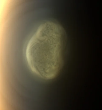
Joshua S. Ford, Nicholas A. Teanby, Patrick G. J. Irwin, Conor A. Nixon, and Lucy Wright

During its flyby of Titan in 1980, Voyager 1 unveiled an atmosphere thick with an opaque, orange haze that completely obscured the surface, and provide  the first close-up images of its vertical layering (Smith et al. 1981, Hanel et al 1981). Subsequent observations from the Cassini-Huygens mission (Flasar et al. 2004) expanded this view, revealing a world dominated by photochemical hydrocarbons and nitriles with lakes of methane  (Stofan et al. 2007, Mastrogiuseppe et al. 2019), tholin-like organic sand (Lorenz et al. 2006), and seasonally evolving ice clouds (Jennings et al. 2012, West et al. 2016) as seen in Figure 1. While recent observations and laboratory studies (Anderson et al. 2011, Chatain et al. 2020) have provided greater insights into the physical properties of these aerosols and how they form, their composition and complexity remain a mystery.

Figure 1: Image taken by Cassini Imaging Science Subsystem (Credit: NASA/JPL-Caltech/Space Science Institute) showing a large ice cloud possibly made of HCN at 300km in Titan’s south pole, 2012 (West et. 2016, Vinatier et al. 2018)

In the upper atmosphere, nitrogen and methane are photodissociated by UV radiation and energetic particles to produce ions which act as embryos for the growth of large organic molecules (Vuitton et al. 2024). As these molecules sink through the atmosphere, they recombine, coagulate, and accumulate into larger aerosol particles, onto which trace species can condense, forming both photochemical hazes and stratospheric ice clouds (Vuitton et al. 2024). 

Cassini CIRS (Composite Infrared Spectrometer) far infra-red spectra (FP1) exhibit four types of hazes: Haze 0, Haze A, Haze B (otherwise known as the “Haystack”) and Haze C (de Kok et al. 2007). While Haze 0 is present throughout the CIRS spectral range and affects the spectral continuum, Haze A, B and C appear as broad features in the far-infrared range. Relatively little is known about these hazes, making their features difficult to fit and estimate. In addition, their signatures overlap with H2O, C4H2, C2N2 and CH4 rotational lines, complicating retrievals of these gases (Sylvestre et al.2017).  Among these hazes, Haze B exhibits the strongest spectral signature. Anderson et al. 2018 suggested that the composition must be a mixture of more than one chemical compound due to its magnitude, breadth and opacity. Haze B is observed to only be present at the winter poles, forming and dissipating with the changing seasons, most likely caused by reduced sunlight and temperature (Jennings et al. 2012a,b , Anderson et al 2018).

To enable accurate fitting of water features, Ford et al. (in review) retrieved an effective spectral cross-section of Cassini CIRS FP1 spectra between 147-257cm-1 of 156 FIRNADCMP 0.5cm-1 observations (Figure 2) across different latitudes and times (see also Ford et al. 2025). This was achieved by scaling gaussian basis functions to fit Haze A, B and C (and any other unknown aerosols) in the spectra baselines using the NEMESIS radiative transfer code (Irwin et al. 2008). Previous aerosol cross-sections did not account for latitude or time variation and therefore this technique empirically and agnostically modelled the changing baseline.  In this study, we decomposed those 156 effective spectral cross-sections and extrapolated unique Haze B cross-sections for latitudes of -89° to 88° from June 2004 to April 2017.  We used principal component analysis to determine the number of complete hazes present in the spectral range, finding that Haze B accounts for 98% of the observed variation. We then applied non-negative matrix factorisation to seperate the spectra into two unique and stable components: one representing Haze B, and a second representing a mixture of other haze contributions, along with numerical and spectral noise.

Figure 2: Effective spectral cross-section of all 156 Cassini CIRS FIRNADCMP 0.5cm-1 observations before decomposition. Each colour represents a different observation. The plot shows the variation extent of the Haze B feature at ~220cm-1

Using the maximum Haze B cross-section of each observation as proxy, we find a large increase at the winter poles with the increase during northern spring being nearly twice that of northern winter, consistent with previous investigations. We also find Haze B extends to 60°, different to 70° proposed by Anderson et al. 2018. The results also give an insight into the time of formation/dispersion of Haze B at the poles. We see that Haze B at the south pole forms around 2013, reaching its peak during the summer solstice. The final dissipation of Haze B at the north pole cannot be determined due to limited data. 

References

Anderson, C.M. et al. (2011), Icarus,  212.2, 762-778. DOI: 10.1016/j.pss.2010.10.009

Anderson, C.M. et al. (2018), Organic Ices in Titan’s Stratosphere in Space Science Reviews, 214.8, 125  DOI: 10.1007/s11214-018-0559-5

Chatain, A.  et al. (2020), Icarus, 345, 113741. DOI: 10.1016/j.icarus/2020.113741

Coustenis, A. et al. (1999), Planet Space Science, 47, 1305-1329. DOI:  10.1016/S0032-0633(99)00053-7

de Kok, R. et al. (2007), Icarus, 191, 223. DOI:10.1016/j.icarus.2007.04.003

Flasar, F.M. et al. (2004), Space Science Reviews, 115, 169–297. DOI: 10.1007/s11214-004-1454-9

Ford, J.S. et al. (2025),  EGU General Assembly 2025, Vienna, Austria, EGU25-3741. DOI: 10.5194/egusphere-egu25-3741

Ford, J.S. et al. In review. Titan’s Stratospheric Water: Latitudinal and Seasonal Variation from Cassini CIRS Data and Implications for External Oxygen Sources. PSJ

Hanel, R.A. et al. (1981), Science, 212, 192–200. DOI: 10.1126/science.212.4491.192

Irwin, P.G.J et al. (2008), JQSRT, 109, 1136. DOI: 10.1016/j.jqsrt.2007.11.006

Jennings, D.E. et al. (2012), The Astrophysical Journal Letters, 754, L3. DOI: 10.1088/2041-8205/754/1/L3

Khanna, R.K. (2005), Icarus, 178,165-170. doi:10.1016/j.icarus.2005.03.011

Lorenz, R. et al. (2006), Science, 312, 724–727. DOI: 10.1126/science.1123257

Mastrogiuseppe, M. et al. (2019), Nature Astronomy, 3, 535, DOI: 10.1038/s41550-019-0714-2

Samuelson, R.E. Clouds and aerosols of Titan’s atmosphere, in The Atmospheres of Saturn and Titan. Proc.Int. Workshop, vol. ESA SP-241 (1985)

Smith, B.A. et al. (1981), Science, 212, 163–191. DOI: 10.1126/science.212.4491.163

Stofan, E.R. et al. (2007), Nature, 445, 61–64. DOI: 10.1038/nature05438

Sylvestre, M. et al. (2017), A&A, 609:A64. DOI: 10.1051/0004-6361/201630255

Vinatier, S. et al. (2018),  Icarus, 310, 89-104. DOI: 10.1016/j.icarus.2017.12.040

Vuitton, V. et al. (2024), Chapter 6:Titan’s Atmospheric Structure, Composition, Haze, and Dynamics in Titan after Cassini–Huygens, COSPAR Scientific Symposium Series.

West, R.A. et al, (2016), Icarus, 270, 399-408. DOI: 10.1016/j.icarus.2014.11.038


How to cite: Ford, J. S., Teanby, N. A., Irwin, P. G. J., Nixon, C. A., and Wright, L.: Decomposing Titan’s far-infrared Haze B feature with PCA and NMF analysis, Europlanet Science Congress 2026, The Hague, The Netherlands, 7–11 Sep 2026, EPSC2026-711, https://doi.org/10.5194/epsc2026-711, 2026.

F3.13
|
EPSC2026-795
|
On-site presentation
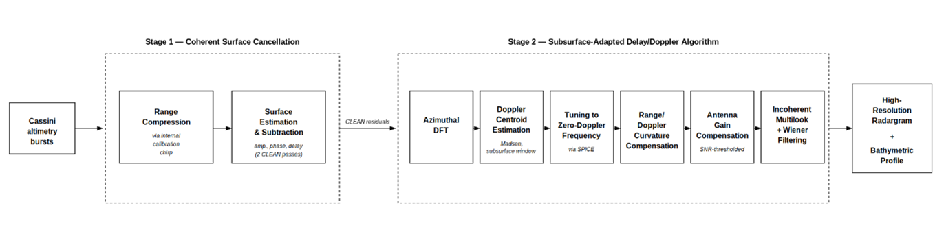
Marco Mastrogiuseppe, Maria Carmela Raguso, Sara Bellucci, Ilaria Rossini, and Daniele Durante
  • Introduction

The Cassini RADAR altimeter (Ku-band, 13.78 GHz, λ ≈ 2.17 cm) provided the first and so far only direct sounding of Titan's hydrocarbon seas, revealing depths exceeding 160 m in Ligeia Mare and constraining the methane-dominated composition of its northern liquid bodies [1–3]. Bathymetric retrievals rely on detecting weak seafloor echoes following the dominant specular surface return. Conventional sidelobe mitigation through spectral windowing (e.g. Blackman tapering combined with Burg autoregressive extrapolation) suppresses sidelobes at the cost of degraded vertical resolution and reduced signal-to-noise ratio (SNR), limiting detections in shallow basins and near shorelines.

We present a re-analysis of Cassini altimetry based on a two-stage processing pipeline that addresses surface dominance directly, without spectral tapering. The pipeline combines (i) a CLEAN-inspired coherent cancellation of the surface return and (ii) a high-resolution Delay/Doppler focusing of the residual subsurface signal. The joint approach preserves the native ~35 m vertical resolution while improving along-track resolution by nearly an order of magnitude. The complete workflow is illustrated in Fig. 1.

Figure 1. Two-stage processing pipeline applied to Cassini RADAR altimetric data. Stage 1 (left): CLEAN-inspired coherent cancellation of the surface return. Stage 2 (right): subsurface-adapted Delay/Doppler processing of the residual bursts. The final products are a high-resolution radargram and an along-track bathymetric profile.

  • Method

Step 1 — Coherent surface cancellation.

For each altimetric burst, the internal calibration chirp—routed directly into the receiver and therefore carrying the full system impulse response—is used as a deterministic replica of the surface return. The complex amplitude, phase, and delay of the surface echo are estimated through cross-correlation between the range-compressed echo and the compressed calibration waveform. A scaled, phase-aligned, and delay-shifted replica of the surface return is then coherently subtracted from the complex waveform on a sample-by-sample basis through CLEAN iterations applied to all bursts. Unlike spectral windowing, this approach removes the dominant surface response without degrading the matched-filter resolution and therefore the SNR.

Step 2 — Subsurface-focused Delay/Doppler processing.

CLEAN-processed residual bursts are focused through a Delay/Doppler Algorithm (DDA) [4,5] adapted for the subsurface regime. The Doppler centroid is estimated within a delay window restricted to the seafloor return, suppressing residual surface contamination, and the burst is retuned to zero-Doppler frequency using SPICE-derived spacecraft state vectors to account for the hyperbolic Cassini flyby geometry. Range/Doppler curvature is then compensated, followed by antenna-gain correction applied selectively to Doppler bins above an SNR threshold, to avoid noise amplification in low-power subsurface regions. Incoherent multilook integration across Doppler-resolved bursts, combined with adaptive Wiener filtering, recovers the SNR loss associated with the reduced number of looks per burst.

  • Results

We apply the pipeline to three Cassini altimetric tracks over Titan's polar terrains — T91 (Ligeia Mare), T108 (Punga Mare), and T126 (Winnipeg Lacus) — and present here Winnipeg Lacus as a representative case study. Results for Ligeia and Punga, including the recovery of the seafloor reflector in shallow regions previously inaccessible to conventional Burg+Blackman processing, will be shown in the accompanying poster.

Winnipeg Lacus (T126).

Winnipeg Lacus is a small polar lake (~78.5°N, 155°W) that lies near the Cassini detection threshold in conventional altimetric processing. After Stage 1, coherent cancellation suppresses the specular surface peak by more than 60 dB and reveals a continuous seafloor reflector across the full track. Stage 2 improves along-track resolution from the beam-limited footprint (~6 km) to the sub-kilometer regime, resolving fine-scale variability of the bottom reflector (Fig. 2). The retrieved bathymetric profile reaches ~105 m maximum depth (estimated uncertainty ±6 m), with an asymmetric morphology — gentle eastern slope and steeper western margin — consistent with erosional processes inferred for Titan's empty lake basins. The retrieved depth is in agreement with the bathymetric profile reported in [3], as shown by the direct comparison in Fig. 3, while the higher along-track sampling of the DDA reconstruction resolves slope variations and basin asymmetries unresolved in the reference profile. The high-resolution radargram supports the methane-rich liquid composition and reveals topographic structures hidden so far by conventional processing, complementing the geophysical characterization of the surrounding northern polar terrains derived from multiangular Cassini RADAR inversion [6].

Figure 2. Winnipeg Lacus (T126 flyby): bathymetric reconstruction. (a) Cassini SAR mosaic with the altimetric ground track (red). (b) Radargram from conventional Burg+Blackman processing: the seafloor reflector is barely discernible against the surface sidelobes. (c) Radargram after coherent surface cancellation (Step 1): the surface peak is suppressed by ~60 dB and the seafloor reflector becomes well-defined. (d) Final radargram after Delay/Doppler focusing (Step 2).

Figure 3. Winnipeg Lacus (T126 flyby). Comparison between bathymetric profiles across the Winnipeg study area. (a) Reference bathymetry from Mastrogiuseppe et al. (2019), with error bars representing the 1σ uncertainty. (b) Bathymetry retrieved using the DDA approach.

  • Conclusions

The combined CLEAN + Delay/Doppler pipeline enables high-resolution bathymetric reconstruction of Titan's hydrocarbon seas without the resolution and SNR degradation of conventional tapering-based methods. Applied to the Cassini altimetry archive, the approach has the potential to extend reliable depth retrievals to previously underutilized flybys and refine constraints on the bathymetry, composition, and connectivity of Titan's seas, with direct implications for Titan's methane cycle and for future missions, including Dragonfly.

References

[1] Mastrogiuseppe M. et al. (2014), Geophys. Res. Lett., 41, 1432–1437. [2] Mastrogiuseppe M. et al. (2018), Earth Planet. Sci. Lett., 496, 89–95. [3] Mastrogiuseppe M. et al. (2019), Nat. Astron., 3, 535–542. [4] Raney R. K. (1998), IEEE Trans. Geosci. Remote Sens., 36(5), 1578–1588. [5] Poggiali V. et al. (2019), IEEE Trans. Geosci. Remote Sens., 57(9), 7262–7268. [6] Mastrogiuseppe M. et al. (2026), IEEE Trans. Geosci. Remote Sens., 64, 4500117.

Acknowledgements

This work was supported by the Italian Space Agency (ASI), contract 2025-4-U.0.

How to cite: Mastrogiuseppe, M., Raguso, M. C., Bellucci, S., Rossini, I., and Durante, D.: High-resolution bathymetry of Titan's hydrocarbon seas through coherent surface cancellation and Doppler focusing of Cassini RADAR altimetry, Europlanet Science Congress 2026, The Hague, The Netherlands, 7–11 Sep 2026, EPSC2026-795, https://doi.org/10.5194/epsc2026-795, 2026.

F3.14
|
EPSC2026-558
|
ECP
|
On-site presentation
Jonas Hener, Dominic Dirkx, Sam Fayolle, Sander Goossens, and Pieter Visser

[Introduction] The existing literature on Titan geodetic parameter estimation from Cassini Doppler data provides an ambiguous view on Titan’s interior and evolution. Recently, three different analyses of this kind have delivered three different (and in parts conflicting) sets of constraints on models of Titan’s interior [1,2,3]. Such parameter estimation analyses involve numerous choices that are rarely documented in full, making it hard to understand, let alone reproduce, published results. Additionally, the analyses are performed using different proprietary software packages. With the present work, we aim to offer a more transparent and accessible analysis of the Cassini-Titan inversion problem and to elucidate the factors underlying differences between previous analyses.

[Method] Using the open-source high-fidelity parameter estimation software Tudat [4], we conduct a systematic simulation study of the inversion problem, in preparation of a full inversion of the Doppler data. As such, this analysis will not present another parameter estimate, but instead studies in a controlled environment the mechanisms that govern the inversion problem. Specifically, we study choices of data selection and weighting, the prior information that is supplied to the filter, and various dynamic models and assess their effect on key geodetic parameters such as the tidal Love number Re(k2) and the static gravity field.

[Results] While many of these aspects significantly affect the formal uncertainty and even the stability with which geodetic parameters are recovered from the inversion, we focus our findings on the treatment of the Titan state estimation. We find that the formal uncertainties of Re(k2), the degree 2 gravity field parameters and even Titan’s gravitational parameter are strongly dependent on how the Titan state is constrained a-priori. We show that choosing prior constraints from a fully independent (astrometry-based) Titan ephemeris solution [5] and applying them in their full form (i.e. including correlations between state parameters) results in more realistic quantification of formal uncertainties and improves the overall stability of the solution. This will also provide important insight towards the fitting of a single consistent Titan orbit across all Cassini flyby arcs. In addition, the lessons learned through our analysis will inform the best practices for the inversion of JUICE’s and Europa Clipper’s multi-flyby and orbit data sets in the Jovian system [6].

We thank V. Lainey for helpful discussions and for providing the covariance matrices of the 2018 JPL/IMCCE Titan ephemeris solution.

[1] Durante, D., et al. (2019). Titan's gravity field and interior structure after Cassini. Icarus, 326
[2] Goosens, S., et al. (2024). A low-density ocean inside Titan inferred from Cassini data. Nature Astronomy, 8(7)
[3] Petricca, F., et al. (2025). Titan’s strong tidal dissipation precludes a subsurface ocean. Nature Astronomy, 648.8094
[4] Dirkx, D., et al. (2022). The open-source astrodynamics Tudatpy software–overview for planetary mission design and science analysis. EPSC2022, (EPSC2022-253).
[5] Lainey, V., et al. (2020). Resonance locking in giant planets indicated by the rapid orbital expansion of Titan. Nature Astronomy, 4(11),
[6] Fayolle, M., et al. (2022). Decoupled and coupled moons’ ephemerides estimation strategies application to the JUICE mission. Planetary and Space Science, 219

How to cite: Hener, J., Dirkx, D., Fayolle, S., Goossens, S., and Visser, P.: Estimating Geodetic Parameters from the Cassini-Titan Orbit Determination Problem: A Systematic Simulation Study, Europlanet Science Congress 2026, The Hague, The Netherlands, 7–11 Sep 2026, EPSC2026-558, https://doi.org/10.5194/epsc2026-558, 2026.