Oral presentations and abstracts

In some of the images taken by OSIRIS, pieces of debris can be seen as bright tracks instead of points sources as result of the combination of movements of both particles and spacecraft. The properties of those tracks, such as orientation, length and total brightness, depend on various comets parameters, including the activity on the nucleus surface, capable of lifting and accelerating the particles, and the characteristics of dust grains, as grain sizes, spatial distribution, velocity, density and sensitivity to radiation pressure. Previous works have focused on retrieving some of these grain properties from the mentioned images, but since the images show the 2D projection of the 3D dust motion, they rely on different methods to obtain the distance between the camera and the debris.

In this work, a new method to bypass this distance determination requirement is proposed. The main steps involved are (i) analyze a large set of images containing tracks generated by moving dust grains, and obtain distribution for selected track parameters (orientation, length, total brightness, etc.) using an algorithm based on the Hough transform method; (ii) compare these results with the ones obtained from artificial images, generated by modeling the three dimensional motion of the debris in the gas flow field of the comet, under the influence of gravity, radiation pressure and gaseous drag; (iii) iterate this process in order to refine the parameters characterizing the physical properties of the dust emission used by the model.

How to cite: Lemos, P.: Statistical analysis of dust grain tracks in Rosetta/OSIRIS images, Europlanet Science Congress 2020, online, 21 Sep–9 Oct 2020, EPSC2020-38, https://doi.org/10.5194/epsc2020-38, 2020.

In August 2019, 2I/Borisov, the second interstellar object and first visibly active interstellar comet, was discovered on a trajectory nearly perpendicular to the ecliptic. Observations of planet forming disks and debris disks serve as probes of the ensemble properties of extrasolar planetesimals, but the passage of an active interstellar comet through our Solar System provides a rare opportunity to individually study these small bodies up close in the same ways in which we investigate objects originating from our own Outer Solar System. Ground-based observations of short period comet 67P/Churyumov–Gerasimenko revealed a coma dust composition indistinguishable from what was measured on its nucleus by the orbiting Rosetta spacecraft. Therefore when 2/I Borisov had a dust dominated tail, we attempted to study its composition with near-simultaneous griJ photometry with the Gemini North Telescope. We obtained two epochs of GMOS-N and NIRI observations in November 2019, separated by two weeks. We will report on the inferred optical-near-IR colors of 2I/I Borisov’s dust coma/tail and nucleus. We will compare our measurements to other observations of 2I/Borisov and place the interstellar comet in context with the Col-OSSOS (Colours of the Outer Solar System Survey) sample of small KBOs and interstellar object ʻOumuamua observed in grJ with Gemini North, using the same setup.

How to cite: Schwamb, M., Bannister, M., Marsset, M., Fraser, W., Pike, R., Snodgrass, C., Kavelaars, J., Benecchi, S., Lehner, M., Peixinho, N., and Fitzimmons, A.: Near-Simultaneous Optical + NIR Photometry of Interstellar Comet 2I/Borisov, Europlanet Science Congress 2020, online, 21 Sep–9 Oct 2020, EPSC2020-46, https://doi.org/10.5194/epsc2020-46, 2020.

Abstract

Institute of Astronomy (University of Latvia) with Ventspils International Radio Astronomy Centre (Ventspils University of Applied Sciences) participation is implementing the scientific project “Complex investigations of the small bodies in the Solar system” related to the research of the small bodies in the Solar system (mainly, focusing on asteroids and comets) using methods of radio astronomy and signal processing. One of the research activities is hydroxyl radical (OH) observation in the radio range - single antenna observations and VLBI (Very Long Baseline Interferometry)  observation. To detect weak (0.1 Jy) OH masers of astronomical objects using radio methods, a research group in Ventspils adapted the Irbene RT-32 radio telescope working at 1665.402 and 1667.359 MHz frequencies. Novel data processing methods were used to acquire weak signals. Spectral analysis using Fourier transform and continuous wavelet transform were applied to radio astronomical data from multiple observations related to weak OH maser detection. Multiple comets (Comet C/2017 T2 (PANSTARRS), Comet C/2019 Y4 (ATLAS), Comet C/2020 F8 (SWAN)) observations were carried out in 2019-2020.

Introduction

There are four known (1612.231,  1665.402, 1667.359 and 1720.530 MHz) hyperfine transitions of OH at 18 cm wavelength which have been used for 40 years, historically to observe comets. In 1973, the molecule OH in comet Kahoutek [1] was observed from the Nancay 30 meter telescope.  The 18 cm line is the result of an excitation from resonance fluorescence, whereby molecules absorb solar radiation and then reradiate the energy. The OH molecule absorbs the UV solar photons and cascades back to the ground state Lambda doublet, where the relative populations of the upper and lower levels strongly depend upon the heliocentric radial velocity (the “Swings effect”) [2]. The result of comets observations in 1.6GHz frequency band made by other astronomy groups [3],[4],[5],[6] and others - show that the typical peak source flux densities of the comet are in the range of 4 to 40 mJy. Weakness of the radio signal is the main challenging factor. Assuming that the detection threshold is 3*σ, at least 1.3 to 13 mJy noise floor  is required. Significant work was invested to prepare the instrumentation of Irbene 32-meter antenna for spectral line observation at L band. This includes improvement of receiver system sensitivity at 1.665 and 1.667 GHz, by building and installing new secondary focus front-end [7].

Observations and data processing

To detect OH masers of the comets, multiple observation sessions were performed using Irbene radio telescope RT32 at 1665.402 and 1667.359 MHz frequencies. Comet Atlas C/2019 Y4 was observed 133 hours, Panstarrs C/2017 - 149 hours, Swan C/2020 F8  - 110 hours. Data calibration and processing methods were necessary to filter out weak OH maser signals from radio astronomical data sets. A programmed USRP X300/310+TwinRX spectrometer is used to record data using 16bit+16bit (real + imag part) per sample. For spectral data calibration, the frequency switching method [8] was integrated in the observation process and data processing was implemented to collect data using long integration time, consequently to perform the compensation of the Doppler shift. For data filtering Fourier transforms, Blackman-Harris window function, Butterworth Low Pass, Locally Weighted Scatterplot Smoothing functions and wavelet transforms were used. Observations of small bodies are possible with the best available accuracy when optical (using the optical Schmidt telescope of Institute of Astronomy) and radio methods are combined [9]. Data processing from two independent simultaneous measurements (using specific Kalman filters) allows one to reduce human errors in sporadic sources. 

Summary and Conclusions

Observations of OH masers of comets can be a very challenging task. The upgrade of the L frequency band receiver was performed in Irbene, Latvia to observe OH masers of comets. Multiple data processing methods were developed to acquire a weak signal. OH masers of the comets (Comet C/2017 T2 (PANSTARRS), Comet C/2019 Y4 (ATLAS), Comet C/2020 F8 (SWAN)) were observed, and the observation process of Comet C/2019 U6, Comet 2P/Encke and Comet C/2020 F3 (NEOWISE) are ongoing in summer 2020.

Acknowledgements

This research is funded by the Latvian Council of Science, project„Complex investigations of the small bodies in the Solar system”, project No. lzp-2018/1-0401.

References

[1] Crovisier, J, et al., Comets at radio wavelengths, C. R. Physique 17 (2016) 985–994 

[2] Despois, D., et al “The OH Radical in Comets: Observation and Analysis of the Hyperfine Microwave Transitions at 1667 MHz and 1665 MHz, Astronomy and Astrophysics, vol. 99, no. 2, June 1981, p. 320-340.

[3] J. Crovisier et al., “Observations of the 18-cm OH lines of comet 103P/Hartley 2 at Nançay in support to the EPOXI and Herschel missions”, Icarus, Volume 222, Issue 2, February 2013, Pages 679-683

[4] B.E.Turner, “Detection of OH at-18-centimeter wavelength in comet KOHOUTEK”, Astrophysical Journal, vol. 189, p.L137-L139

[5] A.J.Lovell et a.l “Arecibo observation of the 18 cm OH lines of six comets”,ESA Publications Division, ISBN 92-9092-810-7, 2002, p. 681 - 684

[6]A. E. Volvach et al. ,”Observations of OH Maser Lines at an 18cm Wavelength in 9P/Temper1 and Lulin C/2007 N3 Comets with RT22 at the Crimean Astrophysical Observatory”, Bulletin of the Crimean Astrophysical Observatory June 2011, Volume 107, Issue 1, pp 122–124

[7] M. Bleiders, A. Berzins., N. Jekabsons, V. Bezrukovs, K. Skirmante, Low-Cost L-band Receiving System Front-End for Irbene RT-32 Cassegrain Radio Telescope, Latvian Journal of Physics and Technical Sciences, 2019, Vol.56, No.3, 50.-61.lpp.

[8] B. Winkel, A. Kraus, and U. Bach. Unbiased flux calibration methods for spectral-line radio observations. Astronomy and Astrophysics, 540:A140, Apr 2012.

[9] K. Skirmante, I. Eglitis, N. Jekabsons, V. Bezrukovs, M. Bleiders, M. Nechaeva and G. Jasmonts, Observations of astronomical objects using radio (Irbene RT-32 telescope) and optical (Baldone Schmidt) methods, Astronomical and Astrophysical Transactions, vol.31, issue 4, 2020

How to cite: Skirmante, K., Bleiders, M., Jekabsons, N., Bezrukovs, V., and Jasmonts, G.: Observations of OH masers of comets in 1.6GHz frequency band using the Irbene RT32 radio telescope, Europlanet Science Congress 2020, online, 21 Sep–9 Oct 2020, EPSC2020-171, https://doi.org/10.5194/epsc2020-171, 2020.

In this work we combine several constraints provided by the crater records on Arrokoth and the worlds of the Pluto system to compute the size-frequency distribution (SFD) of the crater production function for craters with diameter D≤ 10km. For this purpose, we use a Kuiper belt objects (KBO) population model calibrated on telescopic surveys, that describes also the evolution of the KBO population during the early Solar System. We further calibrate this model using the crater record on Pluto, Charon and Nix.  Using this model, we compute the impact probability of bodies with diameter d>2km on Arrokoth, integrated over the age of the Solar System, that we compare with the corresponding impact probability on Charon. Our result, together with the observed density of sub-km craters on Arrokoth's imaged surface, constrains the power law slope of the crater production function. Other constraints come from the absence of craters with 1<D<7km on Arrokoth, the existence of a single crater with D>7km and the relationship between the spatial density of sub-km craters on Arrokoth and of D ~ 20km craters on Charon. Together, these data suggest the crater production function on these worlds has a cumulative power law slope of -1.5<q<-1.2. Converted into a projectile SFD slope, we find -1.2<q_KBO<-1.0. These values are close to the cumulative slope of main belt asteroids in the 0.2-2km range, a population in collisional equilibrium (Bottke et al. 2020). For KBOs, however, this slope appears to extend down to objects a few tens of meters in diameter, as inferred from sub-km craters on Arrokoth. From the measurement of the dust density in the Kuiper belt made by the New Horizons mission, we predict that the SFD of the KBOs become steep again below approximately 30m. All these considerations strongly indicate that the size distribution of the KBO population is in collisional equilibrium.

How to cite: Morbidelli, A., Nesvorny, D., Bottke, W., and Marchi, S.: A re-assessment of the Kuiper belt size distribution for sub-kilometer objects, Europlanet Science Congress 2020, online, 21 Sep–9 Oct 2020, EPSC2020-15, https://doi.org/10.5194/epsc2020-15, 2020.

The Colours of the Outer Solar System Origins Survey (Col-OSSOS, Schwamb et al., 2019) has examined the surface compositions of Kuiper Belt Objects (KBOs) by way of broadband g-, r- and J-band photometry, using the Gemini North Hawaii Telescope. This survey showed a bimodal distribution in the colours of the objects surveyed, consistent with previous colour surveys (Tegler et al., 2016). These broadband surface colours can be considered a proxy for surface composition of these KBOs, so this survey allows the frequency of different surface compositions within the outer Solar System to be explored. The bimodality of the observed colours suggests the presence of some sort of surface transition within the Kuiper belt, perhaps due to a volatile ice-line transition in the pristine planetesimal disk that existed before Neptune’s migration. The Outer Solar System Origins Survey (OSSOS, Bannister et al., 2018), from which Col-OSSOS selected objects brighter than 23.6 r-band magnitude, has well characterised and quantified biases, so allowing for comparisons between the observations and numerical models of the Kuiper belt.

By applying different colour transitions to the primordial planetesimal disk, in this work we explore the possible positions for ice line/colour transitions within the planetesimal disk that existed before Neptune’s migration. Within Schwamb et al. (2019), a simplified toy model was used to investigate the possible position of this transition. Nesvorny et al. (2020) has investigated the primordial colour fraction, in particular how it can create the inclination distribution that we see in the colours of KBOs today. In this work we use a full dynamical model of the Kuiper belt to more precisely pinpoint the possible location of this transition. We make use of the model by Nesvorny & Vokrouhlicky (2016) of Neptune’s migration from 23 au to 30 au, and the consequent perturbation of the Kuiper belt into its current form. This model allows precise tracking of the objects from their pre-Neptune migration to post-Neptune migration positions, allowing various colour transition positions in the initial disk, an example of which is shown in Figure 1, to be compared with the Col-OSSOS observations of the modern day disk.

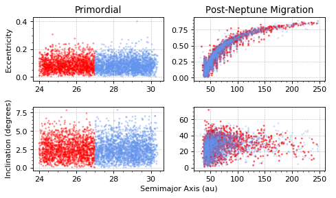
Figure 1: An example red/neutral transition at 27 au. The left plots show the objects in the primordial disk, while the right plots show the objects post-Neptune migration from the model of Nesvorny & Vokrouhlicky (2016).

The OSSOS survey simulator (Lawler et al., 2018) can then be used to calculate which of the simulated objects could have been observed by OSSOS, and so selected by Col-OSSOS for surface colour observations. The colour transition within the initial disk, shown in Figure 1, is moved radially outwards through the disk and the corresponding outputs are compared with the Col-OSSOS colour observations to see which initial disk colour transition positions are consistent with the modern day Kuiper belt. We will present results combing an accurate dynamical model of the Kuiper Belt’s evolution by Nesvorny & Vokrouhlicky (2016) with Col-OSSOS photometry. We will explore multiple radial colour distributions in the primordial planetesimal disk and implications for the the positions of ice line/colour transitions within the Kuiper Belt’s progenitor populations.

References

Bannister, M. T., Gladman, B. J., Kavelaars, J. J., et al. 2018, ApJS, 236, 18
Lawler, S. M., Kavelaars, J. J., Alexandersen, M., et al. 2018, Front. Astron. Space Sci., 5, 14
Nesvorny, D., Vokrouhlicky, D., Alexandersen, M., et al. 2020, AJ, in press
Nesvorny, D., & Vokrouhlicky, D. 2016, ApJ, 825
Schwamb, M. E., Bannister, M. T., Marsset, M., et al. 2019, ApJS, 243, 12
Tegler, S. C., Romanishin, W., Consolmagno, G. J., & J., S. 2016, AJ, 152, 210

How to cite: Buchanan, L., Schwamb, M., Fraser, W., Bannister, M., Marsset, M., Pike, R., Nesvorny, D., Kavelaars, J., Benecchi, S., Lehner, M., Wang, S.-Y., Thirouin, A., Peixinho, N., Volk, K., Alexandersen, M., Chen, Y.-T., Delsanti, A., Gladman, B., Gwyn, S., and Petit, J.-M.: Col-OSSOS: Probing Ice Line/Colour Transitions within the Kuiper Belt's Progenitor Populations, Europlanet Science Congress 2020, online, 21 Sep–9 Oct 2020, EPSC2020-185, https://doi.org/10.5194/epsc2020-185, 2020.

To ensure the safety of a spacecraft and efficiency of the instrument operations it is indispensable to have simple (i.e. with minimal number of parameters and which does not require long time simulations) models for the assessments of the dusty-gas coma parameters. The dusty-gas flow preserves typical general features regardless the particular coma model and the characteristics of the real cometary coma. Therefore, elementary models which account only for the main factors (due to the absence of reliable information on the surface and the interior) affecting the dusty-gas motion could be used for rough estimations of integral characteristics and asymptotic behavior of dusty-gas motion (e.g. terminal velocity, and distance and time when it is reached). At the same time, over-simplification of coma representation is undesirable also. For example, the assumption of spherical symmetry of the flow makes no difference between day and night sides of the coma.

We propose a simple approximation of the gas coma parameters based on the numerical solutions of axisymmetric coma with different activity of the night side (see for example Crifo et al. 2002). This model is given by heliocentric distance r_h, total production rate Q, radius of the nucleus R_n, surface temperature T_n, mechanism of gas production (surface sublimation or diffusion from interior) and level of activity of the night side a_n. This model is able to reproduce typical anisotropy of gas density distribution in real coma and it better conform the physics of real coma than the frequently used model of spherical expansion. In the polar frame with axis directed to the Sun and polar angle φ (solar zenith angle), the spatial distribution of gas density is approximated by third order polynomial of cos(φ):

where coefficients a_i are tabulated for a given mechanism of gas production (surface sublimation or diffusion from interior) and level of activity of the night side a_n. This approximation gives the relative deviation from numerical solution less than 10% in the most part of the coma.

For the dust environment it is assumed that dust grains are spherical homogeneous isothermal particles, non-rotating, with invariable mass (i.e. non-sublimating and noncondensing). The grains released from the surface are submitted to the nucleus gravity F_G, the gas drag F_A, and the solar radiation pressure F_S. We do not allow for solar tidal effects, nor for mutual dust collisions, even though these effects are not always negligible. The theoretical basis of such approach is given in Crifo et al. 2005.

In order to cover a broad range of physical conditions we use dimensionless description of dust dynamics proposed in Zakharov et al. 2018. In this case it is possible to limit the parameter space to three general dimensionless factors Iv, Fu, Ro. The factor Iv characterizes the efficiency of entrainment of the particle within the gas flow; Fu characterizes the efficiency of gravitational attraction; Ro characterizes the contribution of solar radiation pressure. In contrast to the gas environment, the structure of the dust environment can change drastically depending on the particular combination of Iv, Fu, Ro. Therefore, the spatial distribution of dust density can be approximated only for separate combinations of Iv, Fu, Ro within a certain range. The present study covers the range of 5·10^-6 < Iv < 0.1, 10^-7 < Fu < 3·10^-7, 1.5·10^-10 <Ro < 6·10^-6 (i.e. 10^-3 < Ro/Fu < 40.0). For the dust density along sunward direction we propose the approximation:

where coefficients b_i are tabulated for a given mechanism of gas production (surface sublimation or diffusion from interior) and level of activity of the night side a_n. This approximation gives the relative deviation from numerical solution less than 5% for n=4 and 17% for n=3.

Acknowledgements:

This research was also supported by the Italian Space Agency (ASI) within the ''Partecipazione italiana alla fase 0 della missione ESA Comet Interceptor'' (ASIINAF agreement n.Accordo Attuativo" numero 2020-4-HH.0 ).

References:

Crifo,J.F., Lukianov,G.A.,  Rodionov,A.V.,  Khanlarov,G.O., Zakharov, V.V., Comparison between Navier–Stokes and Direct Monte–Carlo Simulations of the Circumnuclear Coma. I. Homogeneous, Spherical Source, Icarus 156, 249–268, 2002.

Crifo, J.-F., Loukianov, G.A., Rodionov, A.V., Zakharov, V.V., Direct Monte Carlo and multifluid modeling of the circumnuclear dust coma Spherical grain dynamics revisited. Icarus 176, 192–219, 2005.

Zakharov, V.V., Ivanovski, S.L., Crifo, J.-F., Della Corte, V., Rotundi, A. , Fulle, M., Asymptotics for spherical particle motion in a spherically expanding flow, Icarus, Volume 312, p. 121-127, 2018.

How to cite: Zakharov, V., Rodionov, A., Fulle, M., Ivanovski, S., Bykov, N., Della Corte, V., and Rotundi, A.: Practical relations for assessments of the dusty-gas coma parameters, Europlanet Science Congress 2020, online, 21 Sep–9 Oct 2020, EPSC2020-223, https://doi.org/10.5194/epsc2020-223, 2020.

Narrow and dense rings have been detected around the small Centaur body Chariklo (Braga-Ribas et al. 2014), as well as around the dwarf planet Haumea (Ortiz et al. 2017).

Both objects have non-axisymmetric shapes that induce strong resonant effects between the rotating central body with spin rate Ω and the radial epicyclic motion of the ring particles, κ. These resonances include the classical Eccentric Lindblad Resonances (ELR), where κ = m(n-Ω), with m integer, n being the particle mean motion. These resonances create an exchange of angular momentum between the body and the collisional ring, clearing the corotation zone, pushing the inner disk onto the body and repelling the outer part outside of the outermost 1/2 ELR, where the particles complete one orbital revolution while the body executes two rotations, i.e. n/Ω ~ 1/2 (Sicardy et al. 2019)

Here I will focus on higher-order resonances. They may appear either by considering other resonances such as n/Ω ~ 1/3, or the same resonance as above (n/Ω ~ 1/2), but with a body that has a triaxial shape. In this case, the invariance of the potential under a rotation of π radians transforms the 1st-order 1/2 Lindblad Resonance into a 2nd order 2/4 resonance.

Second-order resonances are of particular interest because they force a strong response of the particles near the resonance radius, in spite of the intrinsically small strength of their forcing terms. This stems from the topography of the associated resonant Hamiltonian, which possesses an unstable hyperbolic point at its origin.

The width of the region where this strong response is expected will be discussed for both Chariklo's and Haumea's rings. The special case of the second-order 1/3 resonance will be discussed, as it appears that both ring systems are close to that resonance.

This work is intended, among others, to pave the way for future collisional simulations of rings around non-axisymmetric bodies.

How to cite: Sicardy, B., Renner, S., and El Moutamid, M.: Ring dynamics around the Centaur Chariklo and the dwarf planet Haumea: effects of high-order resonances , Europlanet Science Congress 2020, online, 21 Sep–9 Oct 2020, EPSC2020-295, https://doi.org/10.5194/epsc2020-295, 2020.

Abstract

During a two year period between 2014 and 2016 the coma of comet 67P/Churyumov-Gerasimenko (67P/C-G) has been probed by the Rosetta spacecraft. Density data for 14 gas species was recorded with the COmet Pressure Sensor (COPS) and the Double Focusing Mass Spectrometer (DFMS) being two sensors of the ROSINA instrument. The combination with an inverse gas model yields emission rates on each of 3996 surface elements of a surface shape for the cometary nucleus.

The temporal evolution of gas production, of relative abundances, and peak productions weeks after perihelion are investigated. Solar irradiation and gas production are in a complex relation revealing features differing for gas species, for mission time, and for the hemispheres of the comet. This characterization of gas composition allows one to correlate 67P/C-G to other solar and interstellar comets, their formation conditions and nucleus properties, see [3].

Gas production

We analyze in-situ density data of the two sensors COPS and DFMS (see [1]) for the 14 major and minor gas species H₂O, CO₂, CO, H₂S, O₂, C₂H₆, CH₃OH, H₂CO, CH₄, NH₃, HCN, C₂H₅OH, OCS, and CS₂ between August 1st 2014 and September 5th 2016 and heliocentric distances r_h between 3.5 au and 1.24 au. Based on the inverse gas model (section below) the temporal evolution of the cometary gas production is evaluated for all 14 gas species, see [5] and [6].

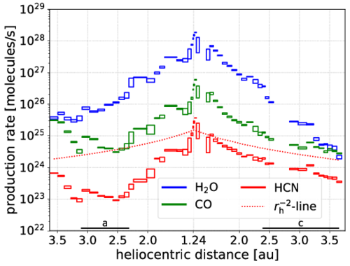
Figure 1: Temporal evolution of the production rates for comet 67P/C-G during the apparition in 2015. The boxes indicate the systematic uncertainties with respect to the limited surface coverage only. The r_h^-2-line specifies a radiation model assuming linear relation between solar irradiation and gas production. The horizontal bars indicate two time intervals I_a and I_c before and after perihelion.

Fig. 1 shows the production rates for the three species H₂O, CO, and HCN complemented by the line for an idealized production assuming a gas production ∼r_h⁻². The H₂O fraction is more than 80 % of the cometary production at peak gas activity during the interval 17 d to 27 d after perihelion. During the time interval I_c from 190 d to 380 d after perihelion, the productions for H₂O, O₂, CH₃OH, H₂CO, and NH₃ follow power laws r_h^α with α ≤ −4.5. A linear relation between solar irradiation and gas production at that time can be excluded for these gases. The group of gases containing CO₂, CO, H₂S, CH₄, HCN, C₂H₅OH, OCS, and CS₂ holds higher exponents −3 ≤ α (see CO and HCN in Fig. 1) in interval I_c. Restricted to the southern hemisphere, the exponents α further approach −2 such that a linear relation between solar irradiation and gas production can be assumed.
As shown in Fig. 1 during the time interval I_a from -290 d to -180 d before perihelion the gases CO and HCN show a significant production decrease although solar irradiation increases at the same time. CO₂, H₂S, O₂, and C₂H₆ remain nearly constant during I_a. [2] report production decrease for CO and stagnation for HCN on comet C/1995 O1 Hale-Bopp which might be explained by interacting sublimations of two different gas species.

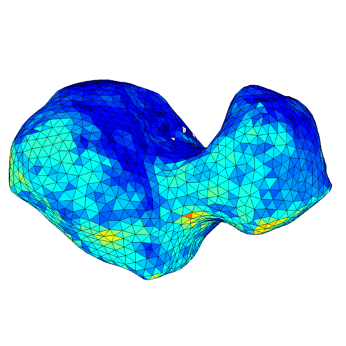
Figure 2: Nucleus of comet 67P/C-G approximated with 3996 triangular elements. Colors indicate source strength of H₂O two weeks after perihelion August 2015.

Model and data analysis

Gas density data of the sensors COPS and DFMS are applied to a simplified inverse gas model for collisionless gas expansion around the nucleus of 67P/C-G, see [4]. Each triangular surface element of a shape model with 3996 elements (see Fig. 2) holds a single gas source described by [7]. Within each of 50 time intervals lasting 9 d to 29 d, each source holds a constant emission rate. Numerical efficiency allows to fit all emission rates on the elements, in all intervals, and for all gases on the HLRN-IV supercomputer.

Summary

The temporal evolution of the gas production of comet 67P/C-G for 14 gas species for a two year period during the apparition 2015 is evaluated. Solar irradiation and production are in a complex relation and show different phenomena. For a number of gases, including CO₂, production is close to a r_h^-2 law, during parts of the outbound mission. For other gases, including H₂O, steeper gradients hold. Inbound CO and HCN hold decreasing production with increasing irradiation at the same time.

Acknowledgements

The work was supported by the North-German Supercomputing Alliance (HLRN). Rosetta is an European Space Agency (ESA) mission with contributions from its member states and NASA. We acknowledge herewith the work of the whole ESA Rosetta team. Work on ROSINA at the University of Bern was funded by the State of Bern and the Swiss National Science Foundation.

References

[1] Balsiger H., et al., 2007, Space Science Reviews, 128, 745
[2] Biver N., et al., 2002, Earth, Moon, and Planets, 90, 5
[3] Bodewits D., et al., 2020, Nature Astronomy
[4] Kramer T., Läuter M., Rubin M., Altwegg K., 2017, MNRAS, 469, S20
[5] Läuter M., Kramer T., Rubin M., Altwegg K., 2019, MNRAS, 483, 852
[6] Läuter M., Kramer T., Rubin M., Altwegg K., 2020, MNRAS, submitted
[7] Narasimha R., 1962, J. Fluid Mech., 12, 294

How to cite: Läuter, M., Kramer, T., Rubin, M., and Altwegg, K.: Gas production for 14 species on comet 67P/Churyumov-Gerasimenko from 2014-2016, Europlanet Science Congress 2020, online, 21 Sep–9 Oct 2020, EPSC2020-319, https://doi.org/10.5194/epsc2020-319, 2020.

Introduction. Pluto was first identified in 1930 and since that time has completed less than 40% of its orbit (248 Earth-years). Studies of Pluto's surface composition have been ongoing for only a small subset of this period, beginning with the first evidence for CH₄ (methane) ice on the surface [1] only a few years before Pluto reached equinox in 1988 and perihelion in 1989. Therefore, the majority of spectroscopic studies have taken place during northern hemisphere spring, as Pluto recedes from the Sun. Since Pluto has a ~122° obliquity and an eccentric (e=0.25) orbit, these seasonal transitions ought to be extreme [2] and potentially observable over time. Simulations of Pluto's surface evolution suggest that the entire northern hemisphere, except for Sputnik Planitia, will be devoid of volatile ices (N₂, CO, CH₄) by 2030 [3]. Given that in 2015 New Horizons saw extensive deposits of volatile ices in the northern hemisphere [4,5] the removal process must occur relatively rapidly, if the models are correct. The duration of the New Horizons flyby was too brief to observe large-scale changes in surface composition or ice distribution.

Observations. One method for evaluating changes on Pluto on timescales of a few years while accounting for rotational variability is to obtain spectra at the same sub-observer latitude and longitude roughly a year apart [6]. This cadence is made possible by the inclination of Earth's orbit with respect to the ecliptic, which presents a limited range of sub-observer latitudes on Pluto repeating ~14 months later. In order to quantify Pluto's short-term surface changes, while correcting for its rotational variability, we designed a spectroscopic observing program specifically to make use of these “matched pairs.” Pluto was observed on 13 nights between June 2014 and August 2017 using TripleSpec, a cross-dispersed spectrograph [7] at the Apache Point Observatory’s Astrophysical Research Consortium 3.5-meter telescope. These spectra were obtained at an average resolving power of ~3500 from 0.91 to 2.47 μm. Matched pairs typically corresponded to spectra obtained in June of one year and August of the next year, at roughly the same (±10°) sub-observer longitude, avoiding opposition where the viewing geometry at small phase angles affects band depth and width [8]. Pluto’s solar phase curve is also relatively flat between phase angles of 0.5-1.5° [9], the range over which the matched pair components were acquired. Therefore, any differences in viewing geometry do not significantly affect the spectra.

Analysis and Results. To evaluate changes in surface composition over time, we computed integrated band areas for the 1.16, 1.19, 1.33, 1.66, and 1.72 μm CH₄ absorption features in each of the corrected nightly spectra. We also calculated shifts in the band centers for the same features as a proxy for the amount of N₂ in solution with CH₄ [10]. The changes in CH₄ band depth and band center position for each matched pair (later date minus newer date) are presented in Figures 1 and 2, respectively. Only those changes detected at ±5-σ for band depth and ±3-σ for band center shift were considered statistically significant. The only significant changes were detected between 2014-06-17 and 2015-08-19, centered on a sub-observer longitude of ~280°, which showed an increase in CH₄ band areas as well as a blueshift in the band centers. No other matched pair showed a significant change over the corresponding time period.

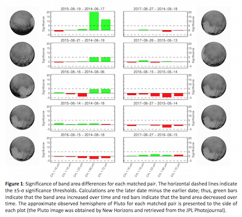
Discussion. Due to scheduling and weather, the majority of the matched pairs were obtained of the anti-Charon hemisphere, home to the bright, volatile-rich Sputnik Planitia. However, the only sub-observer hemisphere with a statistically significant band area increase included only a small portion of Sputnik but a large portion of the low-albedo, volatile-poor Cthulhu Macula [4,5]. The sub-observer hemisphere for the 2015-08-19/2014-06-17 matched pair was unique and contained the largest fraction of Cthulhu Macula.

The increase in CH₄ band areas and the blueshifting of the band centers in the spectra of one unique sub-observer hemisphere between June 2014 and August 2015, and the lack of strong evidence for any decrease in band areas on any sub-observer hemisphere, points to real short-term changes in Pluto's surface composition over this time frame. The lack of significant detections on other hemispheres centered on Sputnik does not necessarily indicate a lack of changes on those hemispheres. Sputnik is a large reservoir of volatile ices that models suggest undergoes little change over a Pluto orbit [3], so the spectra of these sub-observer hemispheres should be dominated by Sputnik’s contribution, drowning out smaller changes on other areas of the surface. Conversely, the 2015-08-19/2014-06-17 sub-observer hemisphere contains a large portion of the volatile-depleted Cthulhu Macula, which would amplify the same changes in surface composition in the spectra.

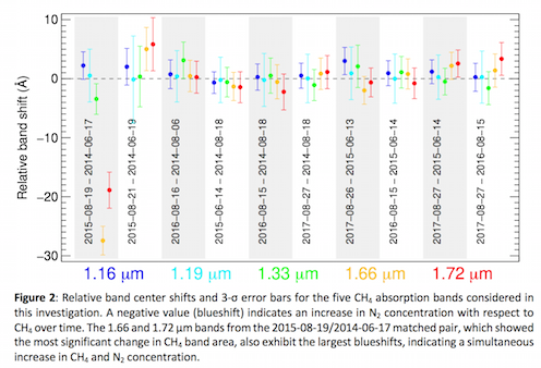
On the sub-observer hemispheres not dominated by Sputnik, volatile N₂ and CH₄ ices are present primarily in the north polar region, with alternating latitudinal bands of CH₄ diluted with N₂ (55-90° N and 20-35° N) and N₂ diluted with CH₄ (35-55° N), as measured by New Horizons in 2015, about one month prior to the second half of the 2015-08-19/2014-06-17 matched pair [5]. The observed changes in the spectra of this sub-observer hemisphere indicate both an increase in CH₄ concentration and an increase in N₂ concentration in the north polar regions. While this sounds contradictory, it can be achieved by preferential sublimation of more-volatile N₂ from latitudes northward of 55° as Pluto approaches northern hemisphere summer, resulting in an increase in CH₄ concentration in those regions, combined with deposition of that N₂ onto the latitudinal band from 35-55°.

References.

[1] Cruikshank, D.P., et al., 1976. Science 194, 835-837. [2] Binzel, R.P., et al., 2017. Icarus 287, 30-36. [3] Bertrand, T., Forget, F., 2016. Nature 540, 86-89. [4] Grundy, W.M., et al., 2016. Science 351, aad9189. [5] Protopapa, S., et al., 2017. Icarus 287, 218-228. [6] Grundy, W.M., et al., 2013. Icarus 223, 710-721. [7] Wilson, J.C., et al., 2004. SPIE 5492, 1295-1305. [8] Pitman, K., et al., 2017. P&SS 149, 23-31. [9] Verbiscer, A., et al., 2019. EPSC-DPS2019-1261. [10] Protopapa, S., et al., 2015. Icarus 253, 179-188.

How to cite: Holler, B., Yanez, M., Young, L., Protopapa, S., Verbiscer, A., and Chanover, N.: Evaluating Temporal Evolution of N2 and CH4 Ices on Pluto with APO/TripleSpec from 2014-2017, Europlanet Science Congress 2020, online, 21 Sep–9 Oct 2020, EPSC2020-336, https://doi.org/10.5194/epsc2020-336, 2020.

A fraction of near-Earth asteroids has the orbital elements similar to those of comets, but a visual aspect as any other point-like source. These are potentially dormant comets nuclei who entered in a period of inactivity. Their study can provide a new understanding of the final state in which volatile-rich objects reside and of the existing organic material or water content distribution from the early Solar System.

Dynamically, cometary orbits can be filtered by their Tisserand parameter with respect to Jupiter (T_Jup). With few exceptions, comets have T_Jup < 3 while asteroids displays T_Jup > 3. Although the value of T_Jup can indicate whether or not the asteroid crosses the Jupiter's orbit, this is not enough to outline a cometary orbit. Tancredi (2014) had developed a method to classify asteroids on cometary orbits (ACOs), based only on orbital elements, which doesn't require any numerical time integration. Beside Tisserand criterion, this algorithm rejects all samples in mean-resonant motion, with large orbital uncertainties and with large minimum orbital intersection distances (MOID) among giant planets.

We seek to make a statistical analysis of the potentially dormant (extinct) comets from near-Earth objects population (NEACOs), using the spectral observations over the visible and near-infrared wavelength interval. The aim of this work is to constraint the fraction of dormant comets orbiting in the near-Earth space. For this study, we’ve compiled a catalog with 149 spectra of near-Earth asteroids (NEAs) with T_Jup < 3. This sample represents 10% out of all known asteroids which obey the T_Jup criterium (Fig. 1).

Fig 1. Absolute magnitude cumulative distributions of all NEACOs from Tancredi's list of ACOs with respect to all with known taxonomy, to those with T_Jup < 3.1 and to all known NEAs (as of January 30, 2020).

The data include new observations of 26 NEAs and 123 spectra retrieved from the literature. The new measurements were obtained with the 2.5 m Issac Newton Telescope and the Nordic Optical Telescope for the visible region, and with the 3.0 m NASA Infrared Facility Telescope for the NIR interval.

For a simplified analysis we’ve grouped all classes from Bus-DeMeo system into four compositional groups. The silicate-like spectra group is mainly consists of objects from Q / S complex (S-, Sr-, Sq-, Sv- types) and some end-members like O-, R- and A-types. In the carbonaceus-like spectra group we've gathered together C-, X- complexes and B-, D-, T- types. The last two groups consist of basaltic asteroids, corresponding to V-type and of relatively rare spectra (miscellaneous) like K- and L-type.

Figure 2. Taxonomic distribution of NEAs with T_Jup < 3.1

The dominant group is of bodies with carbonaceus-like composition, representing 47.5% (71 / 149): 26 C-complex, 22 X-complex, 17 D-type, 6 B-type. The silicate group represents 47% (70 / 149), with an effective of 66 Q/S-complex, 3 R-type and one pure olivine A-type. We report 3 extreme cases with silicate composition: 2 R-types (466130) 2012 FZ23, (394130) 2006 HY51 and one Sr-type (465402) 2008 HW1. Their T_Jup of 2.3, 2.39 and 2.4 respectively are too small for this compositional group. For (466130) we obtained a NIR spectrum. Also, (394130) have a low recorded albedo (0.071), reaching 980 K to perihelion. Taxonomic distribution of entire catalogue (149 samples), presented in Figure 2, displays a strong variation of compositional ratio between silicate and comet-like objects relative to T_Jup.

Within our sample, we could gather data only for 7 asteroids which obey the criteria of Tancredi (2014). All of them are in the Jupiter Familly Comets orbital class. Their spectra classifies them in the carboanceus-like group: 4 D-type (3552, 85490, 248590, 2001 UU92), 1 C-type (475665), 1 T-type (485652) and 1 Xc-type (506437). We conclude that these 7 bodies are dormant / extinct comets. It is important to note that no object with other taxonomy than carbonaceous chondrite, had passed this enhanced criterion, in agreement with the results of Licandro et al. 2018 (who included part of these objects).

References

[1] Tancredi G., 2014, Icarus, 234, 66
[2] Licandro J., et al. 2018, A&A, 618, A170

Acknowledgements

Part of the data utilized in this publication were obtained and made available by the MITHNEOS MIT-Hawaii Near-Earth Object Spectroscopic Survey. 
This work was developed in the framework of EURONEAR collaboration and of ESA P3NEOI projects. The work of M.P. was supported by a grant of the Romanian National Authority for Scientific Research - UEFISCDI, project number PN-III-P1-1.2-PCCDI-2017-0371. M.P., J.dL. and J.L. acknowledge support from the AYA2015-67772-R (MINECO, Spain), and from the European Union’s Horizon 2020 research and innovation programme under grant agreement No 870403 (project NEOROCKS).

How to cite: Simion, G., Popescu, M., Licandro, J., Vaduvescu, O., and de León, J.: Spectral characterization of near-Earth asteroids on cometary orbits, Europlanet Science Congress 2020, online, 21 Sep–9 Oct 2020, EPSC2020-351, https://doi.org/10.5194/epsc2020-351, 2020.

Introduction

20000 Varuna is one of the most interesting TNOs due to its peculiar physical properties. It rotates relatively fast with a period of 6.3435674 h Santos-Sanz et al. (2013), producing a double-peaked rotational light-curve with a very large amplitude, ~ 0.45 mag, dominated by the body shape (e.g., Jewitt & Sheppard 2002, Lellouch et al. 2002, Hicks et al. 2005, Belskaya et al. 2006). Varuna's area-equivalent diameter is ~700 km (Lellouch et al. 2013) and its estimated density, under the assumption of hydrostatic equilibrium (Chandrasekhar et al. 1987), has a value of ~ 1000 kgm^-3, which is somewhat high compared to other TNOs of similar sizes (Ortiz et al. 2012). 

Observations

We present here a collection of new rotational light-curves from 2005 to 2019, taken from three different observatories in Spain (Sierra Nevada Observatory, Calar Alto Observatory and Roque de los Muchachos Observatory), using telescopes of 1.5-m, 1.23-m and 2.2-m, and 3.6-m diameter, respectively. Additionally, we have included three rotational light-curves from the literature (Jewitt & Sheppard 2002, Lellouch et al. 2002, Hicks et al. 2005) to our study. This data set provides different rotational light-curves in a time span of 19 years. 

Results 

We have detected that the amplitude of the rotational light-curve has evolved over time, producing a considerable change along these 19 years, increasing ~ 0.13 mag. We think that this change is due to a variation in Varuna's aspect angle. We model this variation assuming a simple triaxial shape for Varuna's body. The best fit to the data corresponds to a family of solutions with axial ratios b/a between 0.56 and 0.60, which constrains the pole orientation in two different ranges of solutions (see figure 1).

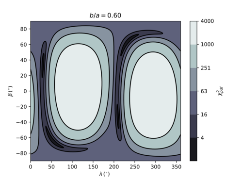
Figure 1. χ² map of possible values for the axis ratio b/a = 0.60. λ_P and β_P are the ecliptic longitude and latitude of the pole orientation (Schroll et al. 1976). The best solution is given by the range λ_P∈[43, 63]º and β_P∈[-70, -58]º (with its complementary direction also possible for the same values of χ²_PDF). Figure from Fernandez-Valenzuela et al. (2019).

Apart from the remarkable variation of the rotational light-curve amplitude along the 19-year time span, we have detected changes in the overall shape of the rotational light-curve in shorter time scales. After the analysis of the periodogram of the residuals to a 6.3435674 h double-peaked rotational light-curve fit, we found a clear additional periodicity (see figure 2). We propose that these changes in the rotational light-curve shape are due to a large and close-in satellite whose rotation induces the additional periodicity. The peak-to-valley amplitude of this oscillation is in the order of 0.06 mag (see figure 3). We estimate that the proposed satellite orbits Varuna with a period of 11.9897 h (or 23.9794 h), assuming that the satellite is tidally locked at a distance of 1300 km (or 2000 km) from Varuna. For more detailed information see Fernandez-Valenzuela et al. (2019).

Figure 2. Lomb periodogram spectral power derived from the residuals of the Fourier function fit to Varuna's photometric data. A maximum spectral power of 45 is obtained at the frequency of 2.003 cycles/day (11.9819 h). This periodicity corresponds to the satellite's revolution period. Figure from Fernandez-Valenzuela et al. (2019).

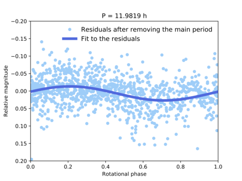
Figure 3. Residuals of Varuna's observational data folded to the 11.9819 h period detected using the Lomb periodogram technique. The blue line represents a one-order Fourier function fit to the points. Figure from Fernandez-Valenzuela et al. (2019).

Acknowlegements: EFV acknowledges UCF 2017 Preeminent Postdoctoral Program (P³). Part of the research leading to these results has received funding from the European Unions Horizon 2020 Research and Innovation Programme, under Grant Agreement No. 687378 (SBNAF). P.S-S. acknowledges financial support by the Spanish grant AYA-RTI2018-098657-J-I00 "LEO-SBNAF" (MCIU/AEI/FEDER, UE). We would like to acknowledge financial support by the Spanish grant AYA-2017-84637-R and the financial support from the State Agency for Research of the Spanish MCIU through the "Center of Excellence Severo Ochoa" award for the Instituto de Astrofísica de Andalucía (SEV- 2017-0709).

How to cite: Fernández-Valenzuela, E., Ortiz, J. L., Morales, N., Santos-Sanz, P., Duffard, R., and Lellouch, E.: Evidence for a close in satellite in the large TNO Varuna, Europlanet Science Congress 2020, online, 21 Sep–9 Oct 2020, EPSC2020-393, https://doi.org/10.5194/epsc2020-393, 2020.

For a long time it was thought that the cyano (CN) radical, observed remotely many times in various stellar and interstellar environments, is exclusively a photodissociation product of hydrogen cyanide (HCN). Bockelée-Morvan et al. (1984) first questioned this notion based on remote observations of comet IRAS-Araki-Alcock. They reported an upper limit for the HCN production rate which was smaller than the CN production rate previously derived by A’Hearn et al. (1983). Even today, this discrepancy observed for some comets is not resolved although many alternative parents have been suggested. Among the volatile candidates, cyanogen (NCCN), cyanoacetylene (HC₃N) and acetonitrile (CH₃CN), according to Fray et al. (2005), are the most promising ones. While cyanoacetylene and acetonitrile are known to be present in trace amounts in comets, as reported for comet Hale-Bopp by Bockelée-Morvan et al. (2000) and for comet 67P/Churyumov-Gerasimenko by Le Roy et al. (2015) and Rubin et al. (2019), the abundance of cyanogen in comets is unknown. Altwegg et al. (2019) were the first to mention its detection in the inner coma of comet 67P/Churyumov-Gerasimenko, target of ESA’s Rosetta mission.

In this work, we track the signatures of cyanogen in the ROSINA/DFMS (Rosetta Orbiter Spectrometer for Ion and Neutral Analysis/ Double Focusing Mass Spectrometer; Balsiger et al. (2007)) data, collected during the Rosetta mission phase. We derive abundances relative to water for three distinct periods, indicating that cyanogen is not abundant enough to explain the CN production in comet 67P together with HCN. Our findings are consistent with the non-detection of cyanogen in the interstellar medium.

A’Hearn M.F., Millis R.L., 1983, IAU Circ., 3802

Altwegg K., Balsiger H., Fuselier S.A., 2019, Annu. Rev. Astron. Astrophys., 57, 113–55

Balsiger H. et al., 2007, Space Science Reviews, 128, 745-801

Bockelée-Morvan D., Crovisier J., Baudry A., Despois D., Perault M., Irvine W.M., Schloerb F.P., Swade D., 1984, Astron. Astrophys., 141, 411-418

Bockelée-Morvan et al., 2000, Astron. Astrophys., 353, 1101–1114.

Fray N., Bénilan Y., Cottin H., Gazeau M.-C., Crovisier J., 2005, Planetary and Space Science, 53, 1243-1262

Le Roy L. et al., 2015, Astron. Astrophys., 583, A1

Rubin M. et al., 2019, MNRAS, 489, 594-607

How to cite: Hänni, N., Altwegg, K., Pestoni, B., Rubin, M., Schroeder, I., Schuhmann, M., and Wampfler, S.: In-situ detection of cometary cyanogen (NCCN), Europlanet Science Congress 2020, online, 21 Sep–9 Oct 2020, EPSC2020-397, https://doi.org/10.5194/epsc2020-397, 2020.

The determination of non-gravitational forces based on precise astrometry is one of the main tools to establish the cometary character of interstellar and solar-system objects. The Rosetta mission to comet 67P/C-G provided the unique opportunity to benchmark Earth-bound estimates of non-gravitational forces with in-situ data. We determine the accuracy of the standard Marsden and Sekanina parametrization of non-gravitational forces with respect to the observed dynamics. Additionally we analyse the rotation-axis changes (orientation and period) of 67P/C-G. This comparison provides a reference case for future cometary missions and sublimation models for non-gravitational forces.

Orbit changes by non-gravitational forces
Among several thousand candidate orbits we have conducted an exhaustive search for the best-fit trajectory ofcomet 67P/C-G to pin down the magnitude and direction of the non-gravitational. Starting from estimates of the non-gravitational Marsden parameters A₁, A₂, A₃ from [1] and [2] (derived from Earth-bound observations of several apparitions of 67P/C-G), we determined an improved solution compatible with Rosetta telemetry [3]
.
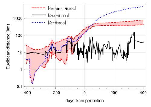
Figure 1: Error for non-gravitational force models for comet 67P/C-G [7]. The label r_ESOC denotes the (noisy) ESA provided orbit, the pink curve the best fit Marsden values, the blue curve is computed without non-gravitational forces (r₀). The reference orbit r_obs shows our best fit to the ESOC data.

Fig. 1 shows that the improved solution reduces the residual error from several hundred kilometers (Marsden parametrization) to about 20 km. This allows us to extract the magnitude anddirection of the non-gravitational acceleration (Fig. 2).

Figure 2: Total magnitude of the non-gravitational acceleration observed for 67P/C-G [7] and water production rate [8]

Comet 67P/C-G displayed a very regular activity pattern with diurnally repeating dust and gas emission [4, 5,6]. This in turn suggests a very uniform non-gravitational acceleration and smooth changes of the rotation axis.

Rotation-state changes
The rotation of comet 67P/C-G shows almost no wobbling motion and changes only by 0.5 DEG over the 2015 apparition [9]. This change is smaller than what a homogeneous emission model (i.e. Keller A model) predicts. In addition it indicates a very close alignment of the axis of inertia with the rotation axis. This requires a slightly inhomogeneous mass distribution with an increased density in the larger lobe.

Summary and Conclusions
We followed the state vector changes of the nucleus of 67P/C-G (momentum and angular momentum) in terms of a Fourier decomposition of the diurnal outgassing in the nucleus-fixed frame. Our analysis constrains the gas release and the inhomogeneity of the near surface ices. For 67P/C-G we find that the standard Marsden parametrization of the non-gravitational forces [10] can be improved considerably. No evidence for a forced precession is seen for 67P/C-G. Our methodology can be applied to other small-bodies with outgassing activity, provided that a shape and initial rotation state is known.

Acknowledgements
The work was supported by the North-German Supercomputing Alliance (HLRN). We acknowledge helpful discussions and joint work concerning the rotational state of 67P/C-G with E. Kührt, H.U. Keller, L. Jorda, andS. Hviid [9].

References
[1] Krolikowska, M. 67P/Churyumov-Gerasimenko - Potential Target for the Rosetta Mission.Acta Astronomica53, 195–209 (2003).
[2] Horizons. Asteroid & Comet SPK File Generation Request. https://ssd.jpl.nasa.gov/x/spk.html (2019).
[3] Godard, B., Budnik, F., Muñoz, P., Morley, T. & Janarthanan, V. Orbit Determination of Rosetta AroundComet 67P/Churyumov-Gerasimenko.Proceedings 25th International Symposium on Space Flight Dynam-ics–25th ISSFD, Munich, Germany(2015).
[4] Kramer, T. & Noack, M. On the origin of inner coma structures observed by rosetta during a diurnalrotation of comet 6P/Churyumov–Gerasimenko.The Astrophysical Journal823, L11–L11 (2016). DOI10.3847/2041-8205/823/1/L11.
[5] Kramer, T., Läuter, M., Rubin, M. & Altwegg, K. Seasonal changes of the volatile density in the coma andon the surface of comet 67P/Churyumov-Gerasimenko.Monthly Notices of the Royal Astronomical Society469, S20–S28 (2017). DOI 10.1093/mnras/stx866.
[6] Kramer, T., Noack, M., Baum, D., Hege, H.-C. & Heller, E. J. Dust and gas emission from cometary nuclei:The case of comet 67P/Churyumov–Gerasimenko.Advances in Physics: X3, 1404436–1404436 (2018).DOI 10.1080/23746149.2017.1404436.
[7] Kramer, T. & Läuter, M. Outgassing-induced acceleration of comet 67P/Churyumov-Gerasimenko.Astron-omy & Astrophysics630, A4 (2019). DOI 10.1051/0004-6361/201935229.
[8] Läuter, M., Kramer, T., Rubin, M. & Altwegg, K.Surface localization of gas sources on comet67P/Churyumov-Gerasimenko based on DFMS/COPS data.Monthly Notices of the Royal AstronomicalSociety483, 852–861 (2019). DOI 10.1093/mnras/sty3103.
[9] Kramer, T.et al.Comet 67P/Churyumov-Gerasimenko rotation changes derived from sublimation-inducedtorques.Astronomy & Astrophysics630, A3 (2019). DOI 10.1051/0004-6361/201834349.
[10] Marsden, B. G. Comets and Nongravitational Forces.The Astronomical Journal73, 367 (1968). DOI10.1086/110640.

How to cite: Kramer, T. and Läuter, M.: Non-gravitational force model vs observation: the trajectory and rotation-axis of comet 67P/Churyumov-Gerasimenko, Europlanet Science Congress 2020, online, 21 Sep–9 Oct 2020, EPSC2020-403, https://doi.org/10.5194/epsc2020-403, 2020.

The most pristine remnants of the Solar system's planet formation epoch orbit the Sun beyond Neptune, the small bodies of the trans-Neptunian object populations.  The bulk of the mass is in ~100 km objects, but objects at smaller sizes have undergone minimal collisional processing, with "New Horizons" recently revealing that ~20 km (486958) Arrokoth appears to be a primordial body, not a collisional fragment.  This indicates bodies at these sizes (and perhaps smaller) retain a record of how they were formed.  However, such bodies are impractical to find by optical surveys due to their very low brightnesses.  Their presence can be inferred from the observed cratering record of Pluto and Charon, and directly measured by serendipitous stellar occultations.  These two methods produce conflicting results, with occultations measuring roughly ten times the number of ~km bodies inferred from the cratering record.  We apply MCMC sampling to explore numerical evolutionary models of the outer Solar system to understand what formation conditions can reconcile the occultations and cratering observations.  We find that models where the initial size of bodies decreases with their semimajor axis of formation, and models where the surface density of bodies increases beyond the 2:1 mean-motion resonance with Neptune can produce both sets of observations.  We discuss the astrophysical plausibility of these solutions, and possible future observations tests of them.

How to cite: Shannon, A., Doressoundiram, A., Roques, F., and Sicardy, B.: Understanding the trans-Neptunian Solar system; Reconciling the results of serendipitous stellar occultations and the inferences from the cratering record., Europlanet Science Congress 2020, online, 21 Sep–9 Oct 2020, EPSC2020-277, https://doi.org/10.5194/epsc2020-277, 2020.

The low-inclination component of the classical Kuiper Belt is thought to be the only population of trans-Neptunian bodies that formed in-situ (Parker et al., 2010). This population, often referred to as the cold classical objects, exhibits a  ~30% observed binary fraction, much higher than for other trans-Neptunian objects (TNOs; Noll et al., 2008). The majority of cold classicals belong to the Very Red (VR) class of the bimodal TNO compositional taxonomy (Fraser and Brown, 2012). Though recently, a population of Less Red (LR) members has been identified, exhibiting a 100% binary fraction (Fraser et al., 2017). These so-called blue binaries are thought to be survivors of a push-out process that occurred during a smooth phase of Neptune’s outward migration. 

Here we report 20 new (g-r) and (r-J) colours of cold classical objects gathered as part of the Colours of the Outer Solar System Origins Survey (Col-OSSOS; Schwamb et al., 2019), bringing the total sample of cold classicals with measured colours to 21 with simultaneous optical and NIR colours, and 103 cold classical TNOs with optical colours alone. In this sample, 29 objects have been identified as binary (Parker, A., personal communication).

Cold classical colours span the full range of optical-NIR colours exhibited by the dynamically excited TNO populations, though they strongly favour red objects;  the VR:LR ratio is ~12 compared to ~3 for the excited TNOs. Moreover, the VR cold classicals have a redder colour distribution than the VR excited TNOs, with the former exhibiting a mean (g-r)~0.95 and the latter, a mean (g-r)~0.8.

The optical colour distribution of binary cold classicals is significantly different than that of the single (or unresolved) cold classical systems (see Figure 1), with the binary sample exhibiting a tail of lower spectral slopes than is found in the sample of singles. The Kolmogorov-Smirnov test comparing the optical colour distributions of the single and binary samples says that there is a only a 0.3% chance the two samples share the same colour distribution. The Col-OSSOS sample on its own shows a similar result, with a 2% probability of the null hypothesis. This argues for a different origin of some or all of the binary cold classicals over the unresolved or single objects population, and is compatible with the hypothesis that the blue binaries are contaminants having been pushed out from regions closer to the Sun.

Figure 1: cumulative optical colour distributions of the single (or unresolved; solid) and binary (dashed) cold classical TNOs. The vertical line demarks the division between less red and very red compositional classes. Spectral slope is reported in percent reddening per 100 nm normalized in the V-band.

How to cite: Fraser, W., Kavelaars, J., Bannister, M., Marsset, M., Schwamb, M., Buchanan, L., Smith, R., Pike, R., Benecchi, S., Lehner, M., Wang, S., and Peixinho, N.: The Colour Distribution Of The Low Inclination Trans-Neptunian Objects, Europlanet Science Congress 2020, online, 21 Sep–9 Oct 2020, EPSC2020-434, https://doi.org/10.5194/epsc2020-434, 2020.

We combine our deep imaging of interstellar comet 2I/Borisov taken with the Hubble Space Telescope/Wide Field Camera 3 (HST/WFC3) on 2019 December 8 UTC and 2020 January 27 UTC (HST GO 16040, PI Bolin) before and after its perihelion passage in combination with HST/WFC3 images taken on 2019 October 12 UTC and 2019 November 16 UTC (HST GO/DD 16009, PI Jewitt) before its outburst and fragmentation of March 2020, thus observing the comet in a relatively undisrupted state. We locate 1-2” long (2,000 - 3,000 km projected length) jet-like structures near the optocenter of 2I that appear to change position angles from epoch to epoch (Fig. 2, left panel). With the assumption that the jet is located near the rotational pole, we determine that 2I's pole points near RA = 322 deg, dec = 37 deg, ecliptic longitude = 341 deg, ecliptic latitude = 48 deg (Fig 2., right panel). We find evidence for periodicity in the time-series lightcurve explained by a nucleus rotation period of ~10.6 h and small amplitude of ~0.05 implying a b/a axial ratio of ~1.5 when combined with our pole solution, unlike the b/a of 4 to 10 found for 1I/`Oumuamua (Bolin et al. 2018). Unless 2I's nucleus was <200 m in size and was spun up rapidly by a pronounced jet after our observations, the March 2020 outburst (Drahus et al. 2020) and fragmentation (Bolin et al. 2020b, Jewitt et al. 2020) was most likely due to calving caused by thermal effects.

References:
Boe et al. 2019. Icarus, Volume 333, p. 252-272., Bolin et al. 2018. ApJL, 852, L2., Bolin et al. 2020a, AJ, 160, 16pp., Bolin et al. 2020b, ATel, 13613., Drahus et al. 2020, ATel, 13549., Fitzsimmons et al. 2019. ApJL, 885, L9., Jewitt et al. 2020, arxiv:2006.01242.

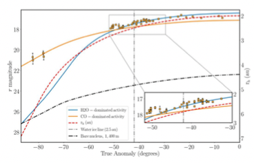
Figure 1. Left panel: r magnitude of 2I as a function of the true anomaly using photometry taken between 2019 March 17 and 2019 November 29 UTC. The blue and orange lines are the predicted brightness as a function of true anomaly angle for H₂O and CO-dominated activity comet from the out-gassing model of 2I from Fitzsimmons et al. 2019. Right panel: the size distribution of ISOs within 3 au of the Sun estimated from the detection of 1I with D~250 m and 2I with D~1.4 km. The solid grey line is fit to data with the function y = ax^b and is based on the estimated size of 1I from the literature and the average of the upper limits on the diameter of 2I assuming 0.04 and 0.1 albedo where a = 0.12 +/- 0.05 and b = 3.38 +/- 1.18.

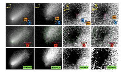
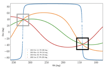
Figure 2. Left panel: Mosaic of radial profile normalized composite images of 2I taken with HST on 2019 October 12 UTC and 2019 November 16 UTC  using the F350LP filter (HST GO/DD 16009, PI Jewitt) and on 2019 December 8 UTC and 2020 January 27 UTC using the F689M and F845M filters (HST GO 16040, PI Bolin) A south-facing jet is observed in the near-nucleus coma in the images taken on 2019 October 12 and 2019 November 16 and a south-west facing jet is observed in the December 8 UTC and 2020 January 27 images (outlined by the dotted purple wedges).  Right panel: Pole/line-of-sight planes from our 4 observing dates. The intersection zone of around RA = 322 deg, dec = 37 deg in the grey square defines the rotation axis with an uncertainty of ~10 degs.

How to cite: Bolin, B., Lisse, C., Kasliwal, M., Quimby, R., Bodewits, D., Morbidelli, A., and Helou, G.: VISIR Characterization of the Nucleus, Morphology, Activity, Spin-Pole Orientation & Rotation of Interstellar Comet 2I/Borisov by Earth- and Space-based Facilities, Europlanet Science Congress 2020, online, 21 Sep–9 Oct 2020, EPSC2020-479, https://doi.org/10.5194/epsc2020-479, 2020.

We present an updated statistical analysis on molecular abundances retrieved from infrared spectra of 20 comets, observed with NIRSPEC-KECK since 1999. Using these results, we investigate the chemical diversity among comets, and we try to correlate them to the chemical and physical processes present during the formation of our planetary system.

Introduction: Comets are considered the remnants of the solar system formation. According to recent dynamical models [1], objects that formed between 5 and 17 AU likely scattered into the Oort cloud (OC), the primary source of long period and dynamically-new comets, while those that formed in the outer proto-planetary disk (beyond 17 AU) entered both the Oort cloud and Kuiper belt (KB) reservoirs. Investigating the chemical diversity in comets may unveil the physical and chemical conditions present during the formation and early evolution of our planetary system (e.g. hydrogenation on dust grains in cold environments or photo-dissociation processes due to UV/X-rays/Cosmic-rays radiation), as well as the processes that may have changed the nucleus composition after its formation (e.g. cosmic rays impacting the outer layer of the nucleus or successive surface warming on repeated passages through the inner solar system).

Since 1985, more than 60 comets have been investigated using ground based high resolution infrared spectrometers, and many efforts have been made to create a classification of these bodies [2,3]. However, some infrared results published before 2011 may contain systematic inaccuracies related to then-incomplete molecular models used to interpret the fluorescence excitation in comets, to a non-properly described atmospheric transmittance models and/or to the use of immature reduction algorithms. These inaccuracies impact mostly comets that were observed before 2011, and they need to be removed [4]. Here, we present a statistical analysis on our revised data for twenty comets and we investigate their possible connections to processes in the proto-planetary disks and/or the natal cloud.

Results and discussion: We have examined the distribution of molecular species among the comet population making use of boxplots (Figure 1). The amount of dispersion that we observe for individual species is expected and could be partially related to the temperature gradient in the proto-planetary disk and/or to the intensity of the radiation field, if present. For instance, the high dispersion range for CO may be related to efficient formation of CH₃OH through hydrogenation processes on dust grains at low temperatures (T < 20 K), or formation of CO₂ at higher temperatures (T > 20 K) [5]. The differential loss of highly volatile species (e.g. CO and CH₄) after the comet formation may also be relevant.

In Figure 2, we show two selected scatterplots for some of the analyzed molecules: these trends should reflect, at least in part, the conditions that were present during the formation of comets. We notice for example that CO shows a high and positive correlation with CH₄, and a much lower but still positive correlation with CH₃OH (an anti-correlation is expected if hydrogenation converted significant CO to CH₃OH). Aspects of the interpretation of the scatterplots will be discussed.

We compared our results with recent disk models [6,7,8], where the relative amounts of CH₃OH, CO, CH₄ and C₂H₆, are expected to depend on what chemical processes and how much radiation field (UV/X/CR) were present at different heliocentric distances from the proto-sun. Considering the combination of these four species (Figure 3), we notice that most of the sampled comets fall in the third and first quadrants and follow an (almost) linear relationship. Depending on the position of the comet with respect to this line, we can define a factor K that can be associated with an increasing processing of the cometary material, and try to reconstruct the chemical and physical history of each analyzed comet.

Conclusions: We report an updated statistical analysis on molecular abundances observed in 20 comets and their possible connections with protoplanetary disk models. The results reveal a diversity in comet composition, and different correlations among the observed chemical species, ultimately giving important hints about the physical and chemical condition present during the formation and evolution of our Solar System.

Figure 1. Boxplot statistic for the chemical species that we observed in 20 comets; for each box we report the interquartile range (IQR), the median (Med), the skewness (Skw), and the whiskers (error bars of the boxplots). Comets characterized by outlier values are highlighted.

Figure 2. Selected scatterplots showing the measured mixing ratios (% with respect to water). For each graphic, the correlation factor is indicated in the upper left corner. Jupiter family and Oort Clouds comets are shown with squares and circles, respectively.

Figure 3: Relationship between relative abundances of selected species and possible connections with the formation and evolution of comets in protoplanetary disks. Jupiter family and Oort Clouds comets are shown with squares and circles, respectively. Colors indicate a possible degree of evolution of the cometary material (violet =  low degree to red = high degree) due to different processes at different life stages of the comet.

This work is supported by the NASA Emerging Worlds Program EW15-57 and the NASA Astrobiology Program 13-13NAI7-0032

References: [1] Morbidelli, A. et al. 2007, Astron. J., 134, 1790; [2] Mumma & Charnley, Ann. Rev A&A, 49, 471 2011; [3] Dello Russo, N. et al. 2016, Icarus, 278, 301; [4] Lippi et al 2020, Astron. J., 159, 157; [5] Tielens, A. G. G. M., Rev. Of Modern Physics, 85, 1021, 2013; [6] Bosman et al. 2018, 618, A182; [7] Walsh 2010 ApJ, 722, 1607; [8] Eistrup et al. 2018, A&A, 613, A14.

How to cite: Lippi, M., Villanueva, G. L., Mumma, M. J., and Faggi, S.: Investigation on the origins of comets as revealed through IR high resolution spectroscopy, Europlanet Science Congress 2020, online, 21 Sep–9 Oct 2020, EPSC2020-495, https://doi.org/10.5194/epsc2020-495, 2020.

Centaurs – planet-crossing bodies in the region of the giant planets that mainly originate in the Kuiper Belt/Scattered Disk [1, 2] – are thought to be the primary impactors on the giant planets and their satellites [3-8]. As part of an effort to interpret the cratering records of the saturnian satellites, we are developing a dynamical-physical model for the size distribution of potential impactors on the moons.

Most models of the orbital distribution of "observable" comets^[1] assume that the size of the nucleus does not change with time. These models treat physical evolution only by assuming a lifetime, after which comets are considered inactive or "faded". These models do not specify a fading mechanism, but assume an expression for the probability that a comet remains active after some amount of time [10-14]. Fading can result from loss of all volatiles, formation of a nonvolatile mantle on the surface of the nucleus, or splitting [15, 16].

A model of the erosion of 67P/Churyumov-Gerasimenko and 46P/Wirtanen due to sublimation of water ice throughout their orbital evolution estimates that 67P’s nucleus has shrunk from a radius of 2.5 km to 2 km, while 46P’s has decreased from 1 km to 0.6 km [17]. This calculation assumes that 10% of the nucleus is active and that its density is 500 kg/m³. These estimates are uncertain because comets follow chaotic orbits, but in general, erosion has a bigger effect on smaller nuclei.

Some comets are active well beyond the water-ice sublimation zone within 3 au. Eighteen active Centaurs are currently known [18, 19]. 29P/Schwassmann-Wachmann, which follows a near-circular orbit at 6 au, is a copious source of dust and CO [20-22] and undergoes significant dust outbursts 7 or more times a year [23]. 174P/Echeclus underwent an outburst 13 au from the Sun that released ≈ 300 kg/s of dust for about two months [24], a rate comparable to the 530 kg/s of dust released by 67P at its peak near 1.3 au [25]. Echeclus also underwent several more outbursts near perihelion (≈6 au) with CO outgassing at ≈ 10% the rate of 29P at the same heliocentric distance and dust mass loss rates of 10 - 700 kg/s [20]. 2060 Chiron is another Centaur that is sporadically active in gas and dust, consistent with a more depleted state, like Echeclus [20].

Di Sisto et al. (2009) constructed a model of the orbital distributions of Jupiter-family comets (JFCs) that incorporated planetary perturbations, nongravitational forces, sublimation, and splitting. They considered nuclei with initial radii of 10, 5, and 1 km [26]. Di Sisto et al. found that 5- and 10-km comets usually evolved onto Centaur orbits, while 1-km comets were most likely to shrink below 100 m. Inspired by their work, we are developing a model for the dynamical-physical evolution of JFCs and Centaurs. We will use the orbital distribution found by Nesvorny et al. as our baseline model [14, 27].

We will first focus on modeling the evolution of the size distribution of JFCs. The model will eventually account for mass loss by both JFCs and Centaurs, with activity driven by H₂O, CO, or other volatiles. The fraction of the nucleus that is active will be allowed to vary with size, since smaller nuclei are typically more active [28-30]. We will then implement a model for cometary splitting with these inputs: the frequency of splitting as a function of perihelion distance; the fraction of the comet’s mass released as fragments; the size distribution of the fragments; and the velocity imparted to the fragments by the splitting event. We will present preliminary results of our simulations.

We thank Raphael Marschall for discussions and the Cassini Data Analysis Program for support.

References

[1] Volk, K.; Malhotra, R. ApJ 687, 714–725, 2008.

[2] Di Sisto, R. P.; Rossignoli, N. L. CMDA, in press (arXiv:2006.09657), 2020.

[3] Zahnle, K.; Dones, L.; Levison, H. F. Icarus 136, 202–222, 1998.

[4] Zahnle, K.; Schenk, P.; Levison, H.; Dones, L. Icarus 163, 263–289, 2003.

[5] Di Sisto, R. P.; Zanardi, M. A&A 553, id. A79, 2013.

[6] Di Sisto, R. P.; Zanardi, M. Icarus 264, 90–101, 2016.

[7] Rossignoli, N. L.; Di Sisto, R. P.; Zanardi, M.; Dugaro, A. A&A 627, id. A12, 2019.

[8] Wong, E. W.; Brasser, R.; Werner, S. C. EPSL 506, 407–416, 2019.

[9] Quinn, T.; Tremaine, S.; Duncan, M. ApJ 355, 667–679, 1990.

[10] Oort, J. H. BAN 11, 91–110, 1950.

[11] Levison, H. F.; Duncan, M. J. Icarus 127, 13–32, 1997.

[12] Wiegert, P.; Tremaine, S. Icarus 137, 84–121, 1999.

[13] Brasser, R.; Wang, J.-H. A&A 573, id. A102, 2015.

[14] Nesvorný, D. et al. ApJ 845, id. 27, 2017.

[15] Weissman, P. R.; Bottke, W. F., Jr.; Levison, H. F. In Asteroids III, Univ. Arizona Press, pp. 669–686, 2002.

[16] Jewitt, D. C. In Comets II, Univ. Arizona Press, pp. 659–676, 2004.

[17] Groussin, O. et al. MNRAS 376, 1399–1406, 2007.

[18] Jewitt, D. AJ 137, 4296–4312, 2009.

[19] Chandler, C. O. et al. ApJLett 892, id. L38, 2020.

[20] Womack, M.; Sarid, G.; Wierzchos, K. PASP 129, 031001, 2017.

[21] Sarid, G. et al. ApJLett 883, id. L25, 2019.

[22] Wierzchos, K.; Womack, M. AJ 159, id. 136, 2020.

[23] Trigo-Rodríguez, J. M. et al. MNRAS 409, 1682–1690, 2010.

[24] Bauer, J. M. et al. PASP 120, 393–404, 2008.

[25] Marschall, R. et al. Frontiers in Physics, doi: 10.3389/fphy.2020.00227 (arXiv:2005.13700), 2020.

[26] Di Sisto, R. P.; Fernandez, J. A.; Brunini, A. Icarus 203, 140–154, 2009.

[27] Nesvorný, D. et al. AJ 158, id. 132, 2019.

[28] A’Hearn, M. F. et al. Science 332, 1396–1400, 2011.

[29] Tancredi, G.; Fernandez, J. A.; Rickman, H.; Licandro, J. Icarus 182, 527–549, 2006.

[30] Schleicher, D. G.; Knight, Matthew M. AJ 152, id. 89, 2016.

How to cite: Dones, L. and Womack, M.: Physical Evolution Model for Jupiter-Family Comets and Centaurs, Europlanet Science Congress 2020, online, 21 Sep–9 Oct 2020, EPSC2020-515, https://doi.org/10.5194/epsc2020-515, 2020.

(90482) Orcus is one of the largest Kuiper belt objects, with one known, relatively large satellite, Vanth. There have been several ~10-20h rotation periods reported in the literature for Orcus, with considerable uncertainty. Here we report on recent measurements of Orcus with the TESS Space Telescope providing a light curve period of 7 h, the fastest rotation among those large trans-Neptunian objects for which the rotation is not expected to cause a distorted, triaxial ellipsoid shape, like in the case of Haumea. While moons of large Kuiper belt objects are usually assumed to be formed from an original large body via collisions, the fast rotation may point to a scenario in which Vanth was captured from a nearby heliocentric orbit early in the history of the Solar system, and subsequent tidal evolution led to the present, nearly circular orbit. In this sense the Orcus-Vanth system is peculiar, as the present rotational characteristics and satellite orbits of all other large Kuiper belt objects are consistent with a collisional origin. 

How to cite: Kiss, C., Pál, A., Szakáts, R., Marton, G., and Müller, T.: The fast rotation of Orcus obtained from TESS measurements, Europlanet Science Congress 2020, online, 21 Sep–9 Oct 2020, EPSC2020-516, https://doi.org/10.5194/epsc2020-516, 2020.

Near-opposition photometry employs remote sensing observations to reveal the microphysical properties of regolith-covered surfaces over a wide range of solar system bodies. When aligned directly opposite the Sun, objects exhibit an opposition effect, or surge, a dramatic, non-linear increase in reflectance seen with decreasing solar phase angle (the Sun-target-observer angle). This phenomenon is a consequence of both interparticle shadow hiding and a constructive interference phenomenon known as coherent backscatter [1-3]. While the size of the Earth’s orbit restricts observations of Pluto and its moons to solar phase angles no larger than α = 1.9°, the opposition surge, which occurs largely at α < 1°, can discriminate surface properties [4-6].

The smallest solar phase angles are attainable at node crossings when the Earth transits the solar disk as viewed from the object. In this configuration, a solar system body is at “true” opposition. When combined with observations acquired at larger phase angles, the resulting reflectance measurement can be related to the optical, structural, and thermal properties of the regolith and its inferred collisional history. The Pluto system was at true opposition when it crossed the line of nodes (Fig. 1) for the first time in 87 years in July 2018 [7], and, owing to the eccentricity of its orbit, it won’t be at true opposition again for another 161 years, in 2179. At the subsequent opposition in July 2019, Pluto was still observable at small phase angles and presented the opposite hemisphere to view.

In 2018, the sunlit portion of Pluto’s Charon-facing hemisphere, centered at longitude 30° E, was observable from Earth at a minimum phase angle α = 0.0049° (Fig. 2). In 2019, its anti-Charon hemisphere was visible at phase angles as small as α = 0.0131°, centered at longitude 210° E, the same hemisphere viewed at high spatial resolution by the New Horizons spacecraft [8]. Since the sub-Earth latitudes were 55° and 56° N in 2018 and 2019, respectively, observations in both years include much of Lowell Regio, Pluto’s bright northern polar cap. Here we present and compare Hubble Space Telescope (HST) near-opposition solar phase curves (Fig. 3) of each of these hemispheres acquired between 2015 and 2019 with the Wide Field Planetary Camera 3 (WFC3) using the UVIS F555W filter (0.53 μm). Since Lowell Regio dominates 60% of the anti-Charon hemisphere and 80% of the Charon-facing hemisphere, the shapes of the two solar phase curves are similar; however, any differences in their shapes reveal differences in the scattering properties and physical surface characteristics of the terrains unique to each hemisphere. The New Horizons encounter (anti-Charon) hemisphere includes Tombaugh Regio and Sputnik Planitia and is ~0.1 magnitudes brighter than the Charon-facing hemisphere in the F555W filter. No part of Sputnik Planitia is visible in the Charon-facing hemisphere, so any differences between its solar phase curve and that of the anti-Charon hemisphere are mainly due to the scattering properties of Pluto’s darker equatorial regions. Preliminary results indicate that the slope of the anti-Charon hemisphere’s phase curve between phase angles 0.3° and 1° (0.025 mag/°) is shallower than that of the Charon-facing hemisphere (0.035 mag/°). When combined with New Horizons LORRI images acquired at higher phase angles, the quantitative analyses of the resulting solar phase curves reveal differences in the structure and texture of regolith particles on Tombaugh Regio and Sputnik Planitia and those on Pluto’s dark equatorial regions, including Cthulhu Macula. 

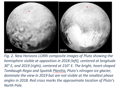
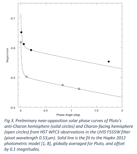
Acknowledgements: Based on observations made with the NASA/ESA Hubble Space Telescope which is operated by the Association of Universities for Research in Astronomy (AURA), Inc., under NASA contract NAS 5-26555. These observations are associated with HST Programs 15505, 15261 (Verbiscer, PI) and 13667 (Buie, PI).

References:

[1] Hapke, B. Theory of Reflectance and Emittance Spectroscopy. Cambridge University Press, 2012. [2] Shkuratov, Yu. & Helfenstein, P. 2001. Icarus 152, 96-116. [3] Hapke, B. 2002. Icarus 157, 523-524. [4] Nelson, R. et al. 2015. LPSC 46, 2584. [5] Verbiscer, A. et al. 2018. In Enceladus and the Icy moons of Saturn. P. Schenk et al., Eds. Univ. Arizona Press, Tucson, p. 323-341. [6] Helfenstein, P. and Shepard, M. 2011. Icarus 215, 83-100. [7] Stern, S. A. et al. 2015. Science 350, aad1815.  [8] Verbiscer, A. et al. 2019. EPSC-DPS 2019 1261.

How to cite: Verbiscer, A., Helfenstein, P., Showalter, M., and Buie, M.: A Tale of Two Sides: Pluto's Opposition Surge in 2018 and 2019, Europlanet Science Congress 2020, online, 21 Sep–9 Oct 2020, EPSC2020-546, https://doi.org/10.5194/epsc2020-546, 2020.

Introduction: The New Horizons flyby of Arrokoth revealed an ancient, contact binary planetesimal [1,2]. Arrokoth’s both lobes’ respective principal axes are aligned within a few degrees [2], and such configuration suggests a co-orbiting Arrokoth before the coalescence of its two lobes [3]. One mechanism proposed for Kuiper belt object (KBO) binaries to merge into a bilobate body is a random walk due to collisions with other heliocentric bodies [3,4]. For Arrokoth, one thing that remains resolved is that its present-day spin period (15.92 hr) is slower than that predicted from both lobes’ mutual gravitational pull (11.26 hr), assuming a comet-nucleus-like density of 500 kg m^-3 [3], implying ~30% angular momentum loss. While Arrokoth may simply be less dense, it is worth exploring whether collisions with other KBOs could have substantially altered its spin state over time. Here we adapt our Monte Carlo impact simulation for Ceres and Vesta [5] and investigate Arrokoth’s possible spindown (or spinup) by impacts.

Triaxial Arrokoth and model results: We previously carried out Monte Carlo impact simulations with random impacts onto an Arrokoth modeled as an oblate spheroid [6]. Here we model Arrokoth as a triaxial ellipsoid by matching its cross-sectional areas along the principal axes with that from its shape model. We also scale this triaxial body’s density for its moment-of-inertia (MOI) to match that of Arrokoth. As a result, this model geometry approximates what the actual Arrokoth would undergo, regarding its dynamical evolution by a given flux of impactors. In this way we avoid the unnecessary complications for trying to track the ejecta interactions on a truly bilobate object.

We base our range of impactor sizes from Arrokoth’s measured craters [2] along with impactor-crater scaling laws [7,8]. While the lower bound is well-determined near 10-m, the upper bound is less well constrained. Both scalings [7,8] predict that the largest crater “Maryland” (~7-km wide, [2]) could have been created by an impactor ~1-to-2-km wide with a typical impact speed ~300 m/s. The total number of impactors is extrapolated from the crater counts [2] where 40-50 craters or pits were recognized during the flyby on one side of Arrokoth. Hence, we allow for 100 impacts between 10 and 1000 m in our simulations (we vary the upper limit later), assuming dN/dD ~ D^-1.75  [2,7], where N(>D) is the number of impactors with diameters greater than D. Implicit in our modeling is the assumption that Arrokoth's craters postdate its (plausibly very early) merger [3]. We also track a disruption energy threshold for porous asteroids [9] to test for potential catastrophic breakup.

Figure 1 consists the results after 5000 Monte Carlo simulations starting at 11.26 hr, with impactors from cold classical KBOs (CCKBOs). No disruption is predicted among all our simulations. About 80% of the simulations end within 11.2 ± 0.2 hr (1σ). Only 2% of the runs have a final spin increase or decrease by more than half an hour. The total, integrated impactor mass is only 0.01 ± 0.01% (1σ) of M, while the total mass loss ejected is 3.8 ± 1.6 times (1σ) larger [10], indicating that Arrokoth is losing mass almost all the time after these 100 impacts. This finding is opposite to what we have found on Ceres or Vesta [5] where a porous surface tends to retain mass rather than losing mass overall; this is expected because the escape velocity of Arrokoth is ~5 m/s, much lower than a typical impact velocity among KBOs [7].

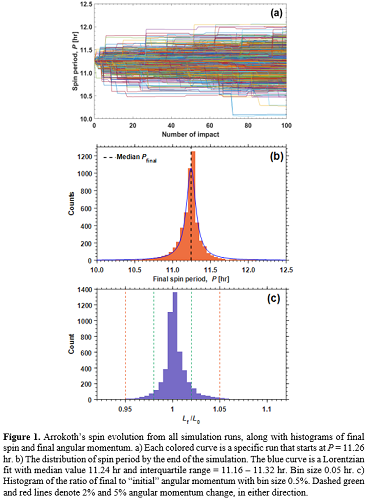
Even though the majority of the impactor flux onto Arrokoth comes from CCKBOs [7], other subpopulations of KBOs also contribute to its overall spin history. Based on pre-encounter model [7], we randomly select ~11% of the impactors to be hot classicals (with a higher impact speed, see Fig. 2); an extra set of 5000 simulations is implemented (Fig. 3). The incorporation of hot classicals delivers notable differences. Due to slightly increased overall impact speed, ejecta loss is further enhanced (about 6.2 ± 5.2 times (1σ) larger than total impactor mass), albeit the net mass change is still ~0.1% M. Whereas the majority of the simulation runs clusters within 1σ from the average, more than 6% experience net spin changes greater than 0.5 hr; indeed, a few runs even achieve the required spindown from 11.26 hr to 15.92 hr. Therefore, Arrokoth’s potential spindown by impacts has a higher likelihood under this condition, although this possibility is still quite low from a statistical point of view.

Discussion: Impacts are shown to play a potentially important role in Arrokoth’s spin angular momentum evolution over time. Our simulations show that major changes of a few hours in spin period, solely by impacts, are highly unlikely, but neither should one assume Arrokoth’s present-day rotation is primordial (or fixed post-merger). The most important role for heliocentric impacts probably occurred when Arrokoth was a co-orbiting binary. The greater the binary separation, the greater the relative angular momentum input to the system for a given impact, the cumulative effect of which could be important for ultimate binary merger. A prior, pre-merger formation of “Maryland” crater could have been especially important for Arrokoth’s angular momentum evolution.

Acknowledgments: This research supported by NASA’s New Horizons project.

References: [1] Stern S.A. et al. (2019) Science 364, eaaw9771. [2] Spencer J.S. et al. (2020) Science 367, aay3999. [3] McKinnon W.B. et al. (2020) Science 367, aay6620.  [4] Nesvorný D. et al. (2018) AJ, 155, 246. [5] Mao X. and McKinnon W.B., MAPS, in revision. [6] Mao X. et al. (2020) 51th LPSC, abs. #2592. [7] Greenstreet S. et al (2019) Astrophys. J. Lett. 872, L5. [8] Housen K.R. et al. (2018) Icarus 300, 72-96. [9] Holsapple K.A. and Housen K.R. (2019) Planet. Space Sci. 179, 104724. [10] Housen K.R. and Holsapple K.A. (2011) Icarus 211, 856-875.

How to cite: Mao, X., McKinnon, W., Singer, K., Keane, J., Robbins, S., Schenk, P., Moore, J., Stern, A., Weaver, H., Spencer, J., Olkin, C., and Science Team, T. N. H.: Investigating Possible Spindown of Arrokoth by Collisions with Small Classical Kuiper Belt Objects, Europlanet Science Congress 2020, online, 21 Sep–9 Oct 2020, EPSC2020-553, https://doi.org/10.5194/epsc2020-553, 2020.

The interstellar comet 2I/Borisov was discovered on August 20, 2019. It is only the second interstellar object to be observed crossing our Solar System, and the first one for which outgassing was detected directly [1]. Early observations indicated that 2I/Borisov is depleted in C₂, similarly to about 30% of Solar System comets [2,3]. Preliminary observations with the MUSE IFU performed in November 2019 confirmed that 2I is depleted in C₂ but also showed it is rich in NH₂ [4]. We present here results from the full observing campaign performed with the MUSE instrument.

MUSE is a multi-unit integral field spectrograph mounted on the UT4 telescope of the VLT [5].  The instrument covers the wavelength range from 480 to 930 nm with a resolving power of about 3000. It has a large field of view of 1’x1’ and a spatial resolution of 0.2”, which makes it an ideal instrument to study extended sources. We observed 2I with MUSE on 16 different dates between November 14, 2019 and March 19, 2020. The observations started about one month before the perihelion passage and continued until the comet reached 3 au post-perihelion. This data sets constitutes a great opportunity to study the activity and coma composition of 2I over several months.

Our observations allow us to detect emission bands from C₂, NH₂, and CN. Using a Haser model [6] we derive production rates for those 3 species and follow their evolution. We also study the evolution of the ratio between those production rates, to monitor how the composition of 2I coma changes as a function of time and distance from the Sun.

References:

[1] Fitzsimmons et al., 2019, The Astrophysical Journal Letters, Volume 885, Issue 1, article id. L9, 6 pp.[2] Opitom et al., 2019, Astronomy & Astrophysics, Volume 631, id.L8, 5 pp.; [3] Lin et al., 2019, The Astrophysical Journal Letters, Volume 889, Issue 2, id.L30;[4] Bannister et al, 2020, submitted to ApJ Letters; [5] Bacon et al, 2010, Proceedings of the SPIE, Volume 7735, id. 773508; [6]  Haser, 1957,Bulletin de la Classe des Sciences de l'Académie Royale de Belgique, vol. 43, p. 740-750

How to cite: Opitom, C., Bannister, M., Rousselot, P., Fitzsimmons, A., Guilbert-Lepoutre, A., Jehin, E., Knight, M., Moulane, Y., Schwamb, M., Seligman, D., Snodgrass, C., and Yang, B. and the the 2I MUSE Observation Team: Follow-up of the activity and composition of the interstellar comet 2I/Borisov with MUSE, Europlanet Science Congress 2020, online, 21 Sep–9 Oct 2020, EPSC2020-569, https://doi.org/10.5194/epsc2020-569, 2020.

Introduction: Comet P/2019 LD2 (ATLAS) was discovered early June 2019 as a faint asteroidal object and initially classified as a Jupiter Trojan. In depth inspection of images obtained during 2019 revealed that the object is active. No signs of cometary-like activity have been detected on any Jupiter Trojans until now, despite it is widely accepted that they are captured objects from the outer solar system. For that reason, we scheduled P/2019 LD2 observations with the world’s largest optical telescope, the 10.4m Gran Telecopio CANARIAS (GTC) to study its nature as soon as it became visible in May 2020

In the meantime, Kareta et al. (2020) showed that the comet had experienced a close encounter with Jupiter on February 17, 2017 at 0.092 AU, well inside the Hill radius of the planet, 0.338 AU. They conclude that it is a recently captured Centaur, not a Jupiter Trojan.

Even if P/2019 LD2 is not the first active Jupiter Trojan, it is a very interesting object that could help to better understand the transition from Centaur to JFC. Its orbit just beyond Jupiter and its activity are evocative of 29P/Schwassmann-Wachmann, an object considered as a prototypical "gateway" between the Centaurs and JFCs by Sarid et al. (2019).

Observations: We present the observations of P/2019 LD2 (ATLAS) obtained on 2020 May 16 and 17 using the OSIRIS camera-spectrograph of the 10.4 m GTC.

On May 16 we obtained images , using the Sloan g’,r’,i’,z’ filters that were used to characterize its overall level of cometary activity using a Monte Carlo dust tail fitting code as described in various papers (see, e.g. Moreno et al. 2016, 2017, and references therein). The comet presents a conspicuous coma and tail as seen Fig. 1.

We also obtained two visible spectra of P/2019 LD2 on May 17 with the aim of looking for signatures of the typical gas species observed in comets. Each individual spectra consisted of an exposure of 600 seconds using the R300B grism and the 1.49′′ slit width, covering a wavelength range from 3600 to 7500 Å, and with a dispersion of 4.96 Å/pix for a 0.6′′ slit.

Fig. 1 Left panel: A comparison of the observed (black contours) and modeled (red contours) tail brightness isophotes. The innermost contour corresponds to 8×10⁻¹⁴ solar disk units, and the brightness decrease in factors of two outwards. The images are rotated to the conventional North- up, East-to-the-left orientation. The x- and y-axis are labeled in km projected on the sky at the object distance. Right panel: A comparison of observed (black line) and modeled (red line) tail brightness along the direction described by the blue dotted line in the left panel.

Past, present and future dynamical evolution: The assessment of the dynamical evolution of P/2019 LD2 requires the analysis of an extensive sample of N-body simulations. In this work, we have used the approach discussed in de la Fuente Marcos & de la Fuente Marcos (2019) and Licandro et al. (2019) to study the past, present and future evolution.

Results: Our results can be summarized as follows:

(i) P/2019 LD2 shows a conspicuous coma and tail with a longitude > 1′.

(ii) There is no evidence of CN, C2 or C3 emission within the 3-σ level in the comet spectrum. In particular there are no signs of the CN (0-0) emission at 3880 Å that it is usually the strongest emission observed in comets.

(iii) According to our model, the dust emission of P/2019 LD2 can be described by a Gaussian with a FWHM=180 days, a maximum (dM/dt)0 = 50 kg s⁻¹ attained on 2019 November 27 (t =170 days from the observations) that then decreases again, with a current (2020 May 16) dust loss rate of 5 kg s⁻¹. This implies a total dust mass loss of 9×10⁸ kg since the start of the dust emission, and almost no dust emission when observed in 2018.

(v) The origin of activity is most likely linked to a thermally driven process, likely associated to sublimation of crystalline water ice and clathrates

(vi) The nucleus corresponds to a km-size object (with radius between 1.5 and 3.5 km), in the size-range of the JFCs.

(vii) P/2019 LD2 is now an ephemeral co-orbital of Jupiter, following what looks like a short arc of a quasi-satellite cycle that started in 2017 and will end in 2028. It will experience a very close encounter with Jupiter at ∼10 Jovian radii on January 18, 2063. If it survive the close approach, its probability of escaping the solar system during the next 0.5 Myr is 0.48±0.02

(ix) The origin of P/2019 LD2 is still an open question. The probability of this comet having been captured from interstellar space during the last 0.5 Myr is 0.50±0.03, 0.79±0.06 during the last 2 Myr and to 0.89±0.07 for 4 Myr, suggesting that P/2019 LD2 can be a captured interstellar comet. Anyhow, a very close encounter with one of the giant planets of a former member of the scattered disk may have produced a fragmentation event induced by the planetary tidal force that was eventually able to form the observed, present-day, P/2019 LD2 .

References

de la Fuente Marcos, C., de la Fuente Marcos, R., Licandro, J., Serra-Ricart, M.,

& Cabrera-Lavers, A. 2019, Research Notes of the American Astronomical

Society, 3, 143

Kareta, T., Volk, K., Noonan, J. W., et al. 2020, Research Notes of the American

Astronomical Society, 4, 74

Licandro, J., de la Fuente Marcos, C., de la Fuente Marcos, R., et al. 2019, A&A,

Moreno, F., Pozuelos, F. J., Novakovic ́, B., et al. 2017, ApJ, 837, L3

Moreno, F., Snodgrass, C., Hainaut, O., et al. 2016, A&A, 587, A155

Sarid, G., Volk, K., Steckloff, J. K., et al. 2019, ApJ, 883, L25

How to cite: Licandro, J., de Leon, J., Moreno, F., de la Fuente Marcos, C., de la Fuente Marcos, R., Cabrera Lavers, A., Lara, L., Pinilla-Alonso, N., de Pra, M., de Souza-Feliciano, A. C., and Geier, S.: The activity of the Jupiter co-orbital comet P/2019 LD2 (ATLAS) observed with the 10.4m GTC., Europlanet Science Congress 2020, online, 21 Sep–9 Oct 2020, EPSC2020-636, https://doi.org/10.5194/epsc2020-636, 2020.

2I/Borisov is the first active interstellar comet observed in the Solar Sytem, allowing for the first time to sample the composition of a planetary building block from an extrasolar system. We report on the monitoring of 2I with the FORS low resolution spectrograph of the ESO VLT at Paranal during four months, from November 19, 2019 to March 20, 2020. We collected a dozen spectra at 8 different epochs allowing to follow the evolution of the comet activity and composition around perihelion. We also observed with the same instrumental setup an Oort Cloud comet, C/2019 U6 (Lemmon), at about the same heliocentric and geocentric distance than 2I/Borisov at perihelion (rh=Delta=2 au) and with similar AfRho value and Q(CN) in order to use it as a reference for the Solar System. The usual species are detected in the optical spectrum of 2I (CN, C3, C2, and NH2) and their production rates and abundance ratios are computed. The dust production rate and colors are also derived, compared to C/2019 U6 and other comets of the Solar System, and their evolutions are followed with the heliocentric distance.

 

Fig1. Comparison of the optical spectra of the interstellar comet 2I/Borisov at perihelion (rh=Delta=2,0 au) and the Oort Could comet C/2019 U6 (Lemmon) observed with FORS at the ESO VLT (Paranal Observatory). C/2019/U6 was chosen for comparison as a Solar System comet with a typical composition. It was also at the about the same distances to the Sun and Earth, and it had about the same dust and CN production rates as 2I/Borisov as measured by the TRAPPIST-South telescope.

How to cite: Jehin, E., Bin, Y., Hainaut, O., Opitom, C., Manfroid, J., Moulane, Y., Fitzsimmons, A., Snodgrass, C., and Meech, K.: Monitoring of the optical spectrum of comet 2I/Borisov at the VLT, Europlanet Science Congress 2020, online, 21 Sep–9 Oct 2020, EPSC2020-653, https://doi.org/10.5194/epsc2020-653, 2020.

Abstract

The processes leading to the formation of planetary systems leave behind a significant mass of small bodies - up to 35 Earth masses depending on the model [1] - orbiting at large heliocentric distance, and observed around 20% of Sun-like stars [2]. It is established that those bodies play an important role in the migration of gas giants away from their stars and may be necessary for life to develop on the smaller planets. Yet, the conditions within these primitive populations are not well understood, especially their collisional environment.

In the last decade, space missions have brought fascinating new data which challenge our concepts of impacts in the Early Solar System. The mission Rosetta at comet 67P, for instance, has revealed a complex cometary world where collisions, from small to catastrophic, played a significant role. Recent work [3,4] suggests that the topography of cometary nuclei and potential layering are shaped by processes which are primarily ancient. Current erosion does not appear sufficient to create features such as deep pits and tall cliffs over the lifetime of a comet in the Inner Solar System. Could they be due to impacts ? Or early activity in the Centaur phase ?

On a larger scale, dynamical simulations argue that objects like the Jupiter Family Comets may have been totally disrupted by catastrophic collisions. While models show that the high porosity and volatile content of cometary nuclei would survive such impacts, it is not clear whether the deeper structural features like layers can be preserved. From the same data set, different authors come to different conclusions with respect to collisions in the early outer planetary system (summarized in [5]). Furthermore, different modeling approaches [6,7,8] lead to distinct results.

Overall, there is quite some confusion as to how to interpret the cratering record on very porous, icy objects, in the Outer Solar System. This is further complicated by the fact that we may not be able to properly recognize impact features on such bodies. 

Here we report on the results obtained by the OCEOSS (Outcome of Collisions in the Early Outer Solar System) ISSI group. The concept of this working group is to bring together experts on collisions and cometary morphology. Over the last few years, modelers have developed new numerical simulations to account for cometary-like material. In parallel, thanks to the Rosetta and New Horizon missions, small bodies morphologists have a much better understanding of the type of landform that can exist on comets, and new measurements of the material physical properties. 

Our group investigates how morphological features observed today on comets and KBOs could relate to the early collisional environment, beyond the typical crater counting studies. 

We will summarize our results along three main topics: Large scale collisions, small scale collisions, and populations. 

We find that the outcome of merger collisions, such as the one which may have created comet 67P or KBO Arrokoth can be very different depending on the internal structure of the bodies. If layers are already present before the collision, the impact may lead to shedding and creation of cliffs/terraces resembling what we see on comets.

More energetic impacts would lead to catastrophic disruption, although the fragments may come back together by gravitational interaction, leading to cometary rubble piles. Recent work on this process for asteroids shows that this could lead to the high porosity and potential density variation we observe across bilobate-comets.

On a local scale, we simulated a km size projectile impacting a 30km KBO, which is the expected order of magnitude for creating features such as the largest crater observed on Arrokoth [9]. We find a large diversity of depth-to-diameter ratio (d/D) for craters, depending on the impact and material parameters. We caution against the simple asteroid-like approximation d/D=10 for all cases [10], as it can lead to erroneous interpretation of the projectile population when extrapolating from crater shapes only.

We will discuss what our models mean for the interpretation of current spacecraft data, and how this work can support future missions to comets/KBOs, like ESA's Comet Interceptor [11].

References:

[1] Tsiganis et al., Origin of the orbital architecture of the giant planets of the Solar System, Nature 2005

[2] Wyatt, M., Extrasolar Kuiper belts, in book The Trans-Neptunian Solar System, 2019

[3] Vincent et al, Constraints on cometary surface evolution derived from a statistical analysis of 67P's topography, MNRAS 2017

[4] Birch et al, Geomorphology of comet 67P/Churyumov-Gerasimenko, MNRAS 2017

[5] Weissmann et al, Origin and Evolution of Cometary Nuclei, SSR 2020

[6] de Niem et al, Low velocity collisions of porous planetesimals in the early solar system. Icarus 2018

[7] Jutzi et al, Formation of bi-lobed shapes by sub-catastrophic collisions. A late origin of comet 67P's structure, A&A 2017

[8] Schwarz et al, Catastrophic disruptions as the origin of bilobate comets, Nature Astronomy 2018

[9] Spencer et al, The geology and geophysics of Kuiper Belt object (486958) Arrokoth, Science 2020

[10] Bottke et al, Interpreting the Cratering History of Bennu, Ryugu, and Other Spacecraft-Explored Asteroids, EPSC 2019

[11] Snodgrass, C. & Jones, G., The European Space Agency's Comet Interceptor lies in wait, Nature Communications 2019

Acknowledgements

The OCEOSS team thanks the International Space Science Institute (ISSI Bern), which made this collaboration possible.

How to cite: Vincent, J.-B., Benavidez, P., Campo-Bagatin, A., Jutzi, M., Kuehrt, E., Luther, R., Michel, P., de Niem, D., Oklay, N., Penasa, L., and Wünnemann, K.: Outcome of Collisions in the Early Outer Solar System, Europlanet Science Congress 2020, online, 21 Sep–9 Oct 2020, EPSC2020-666, https://doi.org/10.5194/epsc2020-666, 2020.

The European Space Agency’s Rosetta mission was designed to orbit and land on the Jupiter-family comet 67P/Churyumov-Gerasimenko (hereafter 67P) for the first time. To investigate the nucleus, the Optical, Spectroscopic, and Infrared Remote Imaging System [1] was designed. The OSIRIS instrument consisted of two cameras operating from near ultraviolet to near infrared wavelengths. The Wide-Angle Camera (WAC) imaged the dust and the gas surrounding the nucleus with a spatial scale of 10.1 m/pixel at 100 km from the surface. The Narrow-Angle Camera (NAC) investigated the comet nucleus and its surface topography with a spatial scale of 1.86 m/pixel at the same distance. The surface of comet 67P immediately appeared geologically complex, with a large variety of terrains and geological features [2]. In addition, the OSIRIS observations revealed a dichotomy in appearance between the two hemispheres. In particular, the northern regions are almost fully covered by dust [2, 3]. On the contrary, in the equatorial regions, consolidated and coarse terrains seem to have replaced the dust on the surface [4]. This dichotomy is linked to the insolation and subsequent erosion of the surface [5]. The dust cover in the northern regions is the result of transport mechanisms of particles from the southern hemisphere during the southern summer [5, 6]. The strong insolation and the water ice content in the south could erode the surface up to 20 m [5] at the perihelion.  

By applying the method developed by Cambianica et al. (2020) [6], we monitored the erosion and accretion of dust deposits of the Imhotep, Hatmehit, and Ma’at regions (Fig. 1) with a vertical accuracy of 0.4 m. The tool is based on the measurement of the shadow length projected by a boulder on the surrounding pebbles deposit. In Fig. 2 an example of the height measurement is shown. After assuming that the position of the boulder did not change during the observational period [7], any height variations provide an indication of how the thickness of the surrounding dust layer is varying in time through erosion and accretion phenomena. We measured the height of three populations of boulders, and the analysis covers the period from August 2014, inbound the perihelion, to September 2016, outbound. Our results show that equatorial regions remain almost inactive before perihelion, contrarily to the Ma’at region which shows erosion during the inbound orbit, and a subsequent dust deposit during the perihelion cometary activity. These results are in line with those found for the Hapi region [6], for which an erosion of the dust deposit of about 1.7 m during the inbound orbit and a fallout of  96% during perihelion cometary activity were measured [6]. Comparing our results with those obtained for the Hapi region, we confirm that the amount of the erosion in the southern hemisphere may be linked with the transport mechanism of the eroded material, and then to its fallout on the nucleus, justifying the presence of coarse terrain only in the southern hemisphere.

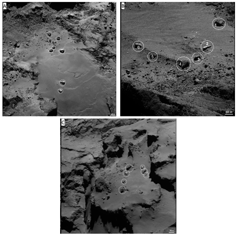
Fig. 1. OSIRIS NAC images showing the analyzed boulder populations located in the Imhotep (A),  Hatmehit (B), and Ma’at (C)  regions of 67P respectively. The first image of this set (A) was taken on 23 November 2014, at a distance of 30.1 km and a scale of 0.57 m/px. Image B was taken on 23 July 2016 at a distance of  10.22 km and has a scale of 0.19  m/px, while the last one (C) was taken on 13 September 2014 at a distance of 30.1 km and a scale of 0.56 m/px. White circles indicate the measured boulders.

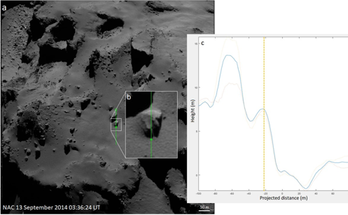
Fig. 2. (a) NAC view of the Ma’at region. This image was acquired in 2014. (b) Close-up of a boulder and of its shadow. The green line represents the projection of the Sun illumination direction. (c) Boulder section. The y-axis is oriented as the normal to the average plane around the peak of the shadow. The x-axis is obtained by projecting the green line in panel b on this average plane; the x-axis origin coincides with the peak of the shadow.

Acknowledgements

OSIRIS was built by a consortium of the Max-Planck-Institut für Sonnensystemforschung, in Göttingen, Germany, CISAS-University of Padova, Italy, the Laboratoire d’Astrophysique de Marseille, France, the Instituto de Astrofísica de Andalucia, CSIC, Granada, Spain, the Research and Scientific Support Department of the European Space Agency, Noordwijk, The Netherlands, the Instituto Nacional de Tecnica Aeroespacial, Madrid, Spain, the Universidad Politechnica de Madrid, Spain, the Department of Physics and Astronomy of Uppsala University, Sweden, and the Institut für Datentechnik und Kommunikationsnetze der Technischen Universität Braunschweig, Germany. The support of the national funding agencies of Germany (DLR), France (CNES), Italy (ASI), Spain (MEC), Sweden (SNSB), and the ESA Technical Directorate is gratefully acknowledged. We thank the ESA teams at ESAC, ESOC and ESTEC for their work in support of the Rosetta mission.

References

[1] Keller, H. U., Barbieri, et al. (2007). Osiris, the scientific camera system onboard Rosetta. Space Science Reviews, 128(1-4):433–506.

[2] Thomas, N., Sierks, H., et al. (2015). The morphological diversity of comet 67P/Churyumov-Gerasimenko. Science, 347(6220):aaa0440

[3] El-Maarry, M. R., Thomas, et al. (2015). Regional surface morphology of comet 67P/Churyumov-Gerasimenko from Rosetta/Osiris images. Astronomy & Astrophysics, 583:A26.

[4] Keller, H. U., Mottola, S., et al. (2017). Seasonal mass transfer on the nucleus of comet 67P/Chuyumov–Gerasimenko. Monthly Notices of the Royal Astronomical Society, 469(Suppl_2):S357–S371.

[5] Keller, H. U., Mottola, et al. (2015). Insolation, erosion, and morphology of comet 67P/Churyumov-Gerasimenko. Astronomy & Astrophysics, 583:A34.

[6] Cambianica, P., Fulle, M., Cremonese, et al., (2020). Time evolution of dust deposits in the Hapi region of comet 67P/Churyumov-Gerasimenko.\ Astronomy and Astrophysics 636, A91.

[7] Cambianica, P., Naletto, G., Cremonese, G. et al. 2019. Quantitative analysis of isolated boulder fields on comet 67P/Churyumov-Gerasimenko.\ Astronomy and Astrophysics 630, A15.

How to cite: Cambianica, P., Cremonese, G., Fulle, M., Simioni, E., Naletto, G., Pajola, M., Lucchetti, A., Penasa, L., and Massironi, M.: Long-term measurements of the erosion and accretion of dust deposits on comet 67P/Churyumov-Gerasimenko with the OSIRIS instrument, Europlanet Science Congress 2020, online, 21 Sep–9 Oct 2020, EPSC2020-724, https://doi.org/10.5194/epsc2020-724, 2020.

In this work, we compare the relationship between the linear phase-function slope (β) and the geometric albedo of Jupiter-family comets (JFCs) to other minor planet populations: Trans-Neptunian objects, Centaurs, Jupiter Trojans, Hilda asteroids, Main-belt asteroids, Near-Earth objects (NEOs), and asteroids on cometary orbits (ACOs). With this analysis, we test whether these two parameters are a good indicator of the surface differences between the various populations and probe whether they can be used to study the surface changes experienced due to the evolution of the various populations.

The albedos and phase functions of small bodies have been used widely to study the surfaces of minor planets throughout the Solar system. However, obtaining both parameters for large samples was difficult in the past. In particular, studies of the surfaces of small bodies focused on the phase-functions’ opposition effect at small phase angles and on the phase integral both of which require well-constrained phase functions that cover a large range of phase angles and careful correction for rotational variability. It is possible, however, to derive the slopes of the linear part of the objects’ phase function with sufficient precision using relatively sparse photometric observations. Moreover, the geometric albedos of large samples of objects have been determined using targeted observations and large surveys in the mid-IR in recent years. Therefore, if the relationship between β and albedo is indicative of the differences in the surfaces of the different populations, it can be used to study a very large number of objects. 

In earlier work, we identified a correlation of increasing albedo for increasing phase-function slope using ground-based and spacecraft observations of 14 Jupiter-family comets (JFCs) [1,2]. This was interpreted as an evolutionary path of JFCs. According to this hypothesis, dynamically young JFCs start their evolution with relatively large albedos and steeper phase functions. Then, during their lifetimes, sublimation-driven erosion gradually makes the comets' surfaces smoother, and their phase-function slopes and albedos decrease.

Interestingly, the correlation identified for JFCs follows the opposite trend to that identified for Main-belt and Near-Earth asteroids (Fig. 1). According to the analysis of Belskaya and Shevchenko (2000) [3] the phase coefficients of asteroids in the range α=5-25° increase linearly as albedo decreases. A similar correlation that also covers lower albedo- and size ranges typical for JFCs was found for NEOs [4]. 

These findings raise two compelling questions. Firstly, if the possible phase-function-albedo correlation for JFCs reflects their sublimation-driven erosion, then can a comparison of JFCs with related populations in the TNOs, Centaurs, and NEOs, and even in the Trojan and Hilda populations be used to reveal more details about the evolution of icy small bodies at different heliocentric distances? Secondly, does the difference in the β-albedo correlation for NEOs and Main-belt asteroids reflect a difference in the surfaces of the two populations, or is it caused by the different size ranges of the objects in the two samples?

We attempted to answer these questions using two lines of investigation. As a first step, we collected objects from all populations with phase-function slopes and albedos in V-band available in the literature. These objects were compared to the JFCs and asteroids in Fig. 1 to check whether they agree with the correlations identified. In the interpretation of this comparison, we took into account the current best understanding of the dynamical history of each population and considered focused studies of individual objects. 

Secondly, in order to study the asteroid phase-function slope-albedo anti-correlation, we collected a larger dataset of Main-belt asteroids, NEOs, ACOs, Jupiter Trojans, and Hildas with albedos known from WISE/NEOWISE (Mainzer et al. 2019) and photometric observations available from the Minor Planet Center. We used this dataset to derive the linear phase-function slope of ~10000 objects from all four populations. Even though the individual phase-function slopes and albedos can have relatively large uncertainties, the large number of objects allow us to characterize the relationship between β and geometric albedo of the individual populations. 

In addition to the findings on the surface properties of the different populations, this work provides useful insights that would serve as a foundation for future phase-function studies (e.g. with the Vera Rubin Observatory’s Legacy Survey of Space and Time; LSST). We will discuss the limitations of the currently available photometric data and will highlight the specific improvements that could be achieved with LSST. 

Fig. 1. Relationship between the linear phase-function slope β and the geometric albedo in V-band for the 14 JFCs in [1,2] (plotted as circles), Main-belt asteroids from [3] (triangles) and NEOs from [4] (squares). The lines correspond to the linear relationships found for each sample. 

[1] Kokotanekova, R. et al. 2017, MNRAS, 471, 2974

[2] Kokotanekova, R. et al. 2018, MNRAS 479, 4665

[3] Belskaya, I. N., & Shevchenko, V. G., 2000, Icarus, 147, 94

[4] Hergenrother, C. et al, 2013, Icarus, Volume 226, Issue 1, p. 663-670. 

[5] Mainzer, A., et al, NEOWISE Diameters and Albedos V2.0., NASA Planetary Data System, 2019.

How to cite: Kokotanekova, R. and Snodgrass, C.: Relationship between the phase-function slope and albedo of comets and asteroids, Europlanet Science Congress 2020, online, 21 Sep–9 Oct 2020, EPSC2020-776, https://doi.org/10.5194/epsc2020-776, 2020.

1. Introduction

To estimate a size-frequency distribution (SFD) of any population of small bodies it is necessary to compensate the observational selection effects, which generally favor larger and brighter objects. For a mixed population, made up of asteroids and comets, as expected for the population of interstellar objects (ISOs), the discovered population should be also significantly biased toward cometary objects, which makes it difficult to estimate even the basic properties of this population. Therefore, the ISO SFD was completely unconstrained [1], until very recent work by Bolin et al. [2].

We have investigated the orbital distribution of ISOs, observable by the future wide-field National Science Foundation Vera C. Rubin Observatory (VRO). The results show that among the asteroidal ISOs, there should be an excess of retrograde orbits among the observed objects [3]. We found that this may be due to the observational selection effects, known as Holetschek’s effect [4]. Interestingly, a level of retrograde orbit excess depends on the SFD of the ISOs, suggesting that the ratio between the prograde and retrograde ISOs observable by the VRO could be used for estimation of the SFD of the underlying true population.

2. Holetschek’s effect

According to this effect, objects which reach perihelion on the side of the Sun opposite to the position of the Earth are less likely to be discovered. This is because in this configuration objects are both, too close to the Sun (small elongation), and further away from the Earth (fainter). Therefore, a probability for an object to be discovered depends on the difference Δλ between the heliocentric longitude of the Earth and that of the object at the time of the perihelion passage of this object. This is illustrated in Fig. 1.

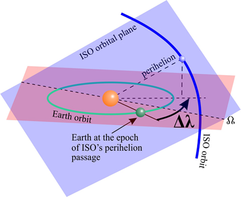
Figure 1 - Constellation related to Holetschek’s effect. Quantity Δλ is the difference between the heliocentric ecliptic longitudes of an interstellar object and the Earth, at the epoch of the object’s perihelion passage.

3. Orbital distribution of ISOs

To investigate the influence of Holetsechek’s effect on ISOs, we generate their synthetic population and simulate their ephemerides over a period of 10 years, in order to select those which may be observed by the VRO, based on the nominal characteristics of this survey. We found that Holetschek’s effect is more pronounced for objects on prograde than for those on retrograde orbits. This is obvious from Fig. 2 in which are shown distributions of Δλ separately for prograde and retrograde objects.

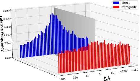
Figure 2 - The normalized histograms of Δλ of the detectable objects. The figure shows separately objects on direct (i<90 deg) and retrograde (i>90 deg) orbits. The vertical plane denotes objects which pass through their perihelions while they are on the same heliocentric ecliptic longitude as the Earth. The observed asymmetry is likely due to Holetschek’s effect.

4. Future prospect

Different sensitivity of prograde and retrograde objects to the effect results in asymmetry of distribution of the orbital inclinations of the detectable population. On the other hand, Holetschek’s effect mostly affects small bodies, while for larger objects (of the order of several km) it is almost negligible. Since populations with steeper size distribution have larger portion of small objects, they are more subjected to this effect, resulting in a more pronounced asymmetry of the distribution of orbital inclinations. Our results show that a retrograde/prograde orbits ratio and median orbital inclination of the detectable population is correlated with the SFD slope of the generated population of ISOs. Therefore, these parameters of the discovered population of ISOs could, in turn, be used to estimate the SFD of the underlying true population. Alternatively, based on an available estimation of the SFD of interstellar objects [2], the expected excess of retrograde orbits could be calculated.

References:

1. Engelhardt T., Jedicke R., Vereš P., Fitzsimmons A., Denneau, L., Beshore E., Meinke B.: 2017, AJ, 153, 133

2. Bolin B.T., et al., 2020, AJ, 160, 26

3. Marčeta D., Novaković B., 2020, MNRAS, doi:10.1093/mnras/staa1378 (arXiv:2005.10236)

4. Holetschek J., 1891, Astronomische Nachrichten, 126, 75

How to cite: Marceta, D. and Novakovic, B.: Can Holetschek’s effect provide a tool for estimating size-frequency distribution of interstellar objects?, Europlanet Science Congress 2020, online, 21 Sep–9 Oct 2020, EPSC2020-787, https://doi.org/10.5194/epsc2020-787, 2020.

The accuracy achieved by modern deep space radio tracking systems has dramatically increased the precision of planetary ephemerides in the last decade. This improvement is particularly beneficial to the study of the trans-Neptunian solar system, still a relatively unknown region (Prialnik et al. 2020).

The Kuiper belt has a pivotal role in our understanding of the outer solar system, and a better constrain of its mass inferred by its gravity perturbations on the planets can help to explain the observed clustering of Kuiper belt objects (KBO), and the potential presence of a ninth planet beyond the orbit of Neptune, P9 (Batygin et al. 2019).

We thus provide a new estimate of the cumulative mass of KBOs located in the 2:1 and 3:2 mean motion resonances with Neptune deduced from INPOP19a. INPOP19a is the last version of INPOP planetary ephemeris, which, among the numerous updates (Fienga et al. 2019), benefits from the addition of the new normal points obtained with the gravity experiment of the Juno mission and the new normal points deduced from Cassini radio tracking data. The latter, in particular, play a decisive role for constraining the mass of the Kuiper belt, thanks to the enhanced accuracy registered in the analysis of navigation and gravity data (Di Ruscio et al. 2020; Durante et al. 2019) and the extended time-frame covered with the inclusion of the Grand Finale measurements (Iess et al. 2019).

We modeled the Kuiper belt by including in INPOP dynamical model three circular, not inclined rings located at 39.4, 44.0, and 47.5 AU, to which we attributed one-sixth, two-thirds, and one-sixth of the total mass, respectively, using the same approach adopted by Pitjeva & Pitjev (2018). In addition, we included the orbits of nine KBOs, beside Pluto, whose masses are independently constrained by observations of their satellites dynamics.

Solving for the mass of the Kuiper belt together with the orbits of the eight planets of the solar system, Pluto, and the Moon, plus the mass of 343 asteroids of the main belt, we fitted the entire INPOP dataset (Fienga et al. 2019) and estimated a total mass for the rings of KBOs of (0.061 ± 0.001)M_⊕.

We also provide new constraints on the location of P9 by analyzing the potential gravity perturbation on planetary ephemerides, specifically on the orbit of Saturn. We used two statistical criteria to identify the possible regions compatible with INPOP19a: i) based on the propagated covariance matrix, and ii) on the χ² likelihood of P9-perturbed postfit residuals (Fienga et al. 2020). We show that, according to INPOP19a, there is no clear evidence for the existence of P9, but we identified two zones for which its existence is compatible with the accuracy of INPOP planetary ephemerides (see Fig. 1).

Fig. 1. The plots show the two compatible zones we identified for the potential location of P9 with a mass of 5 M_⊕ at a distance of 600 AU. The x and y axes report the angular position in Right Ascension (RA) and Declination (Dec) of the planet in the International Celestial Reference Frame. The colorbar indicates the χ² Likelihood computed for each P9-perturbed solution.

References:

Batygin, K., Adams, F. C., Brown, M. E., and Becker, J. C. 2019, “The Planet Nine Hypothesis”, Physics Reports, 805

Di Ruscio, A., Fienga, A., Durante, D., Iess, L., Laskar, J., and Gastineau, M. 2020, “Analysis of Cassini radio tracking data for the construction of INPOP19a: A new estimate of the Kuiper belt mass”, A&A, Forthcoming article

Durante, D., Hemingway, D. J., Racioppa, P., Iess, L., and Stevenson, D. J. 2019, “Titan's gravity field and interior structure after Cassini”, Icarus, 326, 123

Fienga, A., Deram, P., Viswanathan, V., Di Ruscio, A., Bernus, L., Durante, D., Gastineau, M., and Laskar, J. 2019, “INPOP19a planetary ephemerides”, NSTIM, 109

Fienga, A., Di Ruscio, A., Bernus, L. Deram, P., Durante, D., Laskar, J., and Iess, L. 2020, “New constraints on the location of P9 obtained with the INPOP19a planetary ephemeris”, A&A, Forthcoming article

Iess, L., Militzer, B., Kaspi, Y., et al. 2019, “Measurement and implications of Saturn’s gravity field and ring mass”, Science, 364

Pitjeva, E. V. & Pitjev, N. P. 2018, “Mass of the Kuiper belt”, Celest. Mech. Dyn. Astron, 130, 57

Prialnik, D., Barucci, M., and Young, L. 2020, “The Trans-Neptunian Solar System”, Elsevier

How to cite: Di Ruscio, A., Fienga, A., Bernus, L., Deram, P., Durante, D., Iess, L., Laskar, J., and Gastineau, M.: New constraints on the Kuiper belt mass and P9 location from INPOP19a planetary ephemerides, Europlanet Science Congress 2020, online, 21 Sep–9 Oct 2020, EPSC2020-804, https://doi.org/10.5194/epsc2020-804, 2020.

Abstract

During the journey through the solar system, interstellar comet 2I/Borisov has been observed spectroscopically by most of the largest telescopes on Earth, enabling comparative studies of its chemical composition versus solar system comets. Already a few weeks after the discovery, the detection of the CN (0-0 band) in the coma has been reported [1]. Subsequent detections of C₂ suggested a significant depletion of this molecule [2,3], however, later evolution of C₂ placed it close to the typical values [4]. Pre-discovery images of 2I/Borisov showing this object to be active when far away from the sun indicated that its activity is driven by low-temperature volatiles, later confirmed by the detection of a high abundance of CO [5,6]. High abundance was also reported for NH₂ [4]. The water production rates derived from the detection of [OI] 6300 A line [7] were consistent with SWIFT/UVOT observations [8].

Here we report our spectroscopic observations of 2I/Borisov from VLT X-Shooter. We collected over 10 hours of data on UT 2020 January 28th, 30th, and 31st obtaining the deep spectrum of this object taken around the time of its maximum brightness. The spectrum covers an unprecedented wavelength range of 300 - 2500 nm that comprises numerous characteristic cometary emissions. The excellent sensitivity of the spectrum, combined with the decent spectral resolution provided by X-Shooter over the entire, enormous wavelength range makes the collected material unique.

Acknowledgements

Authors are grateful for support from the National Science Centre of Poland through SONATA BIS grant number 2016/22/E/ST9/00109 to M.D.

References

[1] Fitzsimmons, A., Hainaut, O., Meech, K. et al.: Detection of CN Gas in Interstellar Object 2I/Borisov, ApJL, Vol. 885, L9, (2019)
[2] Kareta, T., Andrews, J., Noonan, J. et al.: Carbon Chain Depletion of 2I/Borisov, ApJL, Vol. 889, L38, (2020)
[3] Lin, H., Lee, C., Gerdes, D. et al.: Detection of Diatomic Carbon in 2I/Borisov, ApJL, Vol. 889, L30, (2020)
[4] Bannister, M., Opitom, C., Fitzsimmons, A. et al.: Interstellar comet 2I/Borisov as seen by MUSE: C_2, NH₂ and red CN detections, https://arxiv.org/abs/2001.11605, (2020)
[5] Bodewits, D., Noonan, J., Feldman, P. et al.: The carbon monoxide-rich interstellar comet 2I/Borisov, NatAst, (in press)
[6] Cordiner, M., Milam, S., Biver, N. et al.: Unusually high CO abundance of the first active interstellar comet, NatAst, (in press)
[7] McKay, A., Cochran, A., Dello Russo, N. et al.: Detection of a Water Tracer in Interstellar Comet 2I/Borisov, ApJL, Vol. 889, L10, (2020)
[8] Xing, Z., Bodewits, D, Noonan, J. et al.: Water Production Rates and Activity of Interstellar Comet 2I/Borisov, ApJL, Vol. 893, L48, (2020)

How to cite: Guzik, P. and Drahus, M.: Spectrosopy of interstellar comet 2I/Borisov with VLT X-Shooter, Europlanet Science Congress 2020, online, 21 Sep–9 Oct 2020, EPSC2020-846, https://doi.org/10.5194/epsc2020-846, 2020.

We present the newest iteration of our particle tracking algorithm and highlight findings based on its application to different data sets. The intended use of the algorithm is to analyze image sequences taken by the Optical, Spectroscopic, and Infrared Remote Imaging System (OSIRIS) of the Rosetta spacecraft during the outbound perihelion phase of comet 67P/Churyumov-Gerasimenko. During this active phase, a lot of material was being ejected, in part as relatively large, boulder-sized objects (dm to m). With our work, we hope to better understand the processes that are responsible for the ejection and those that might affect the flight path of the particles once they are lifted. 

How to cite: Pfeifer, M. and Agarwal, J.: Dust Particle Tracking at Comet 67P/Churyumov–Gerasimenko, Europlanet Science Congress 2020, online, 21 Sep–9 Oct 2020, EPSC2020-865, https://doi.org/10.5194/epsc2020-865, 2020.

Abstract

Transneptunian Objects (TNOs) are the remnants of our planetary system and can retain information about the early stages of the Solar System formation. Stellar occultation is a ground-based method used to study these distant bodies which have been presenting exciting results mainly about their physical properties. The big TNO called 2002 MS4 was discovered by Trujillo, C. A., & Brown, M. E., in 2002 using observations made at the Palomar Observatory (EUA). It is classified as a hot classical TNO, with orbital parameters a = 42 AU, e = 0.139, and i = 17.7º. Using thermal measurements with PACS (Herschel) and MIPS (Spitzer Space Telescope) instruments, Vilenius et al. 2012 obtained a radius of 467 +/- 23.5 km and an albedo of 0.051.

Predictions of stellar occultations by this body in 2019 were obtained using the Gaia DR2 catalogue and NIMA ephemeris (Desmars et al. 2015) and made available in the Lucky Star web page (https://lesia.obspm.fr/lucky-star/). Four events were observed in South America and Canada. The first stellar occultation was detected on 09 July 2019, resulting in two positives and four negatives chords, including a close one which proven to be helpful to constrain the body’s size. This detection also allowed us to obtain a precise astrometric position that was used to update its ephemeris and improve the predictions of the following events. Two of them were detected on 26 July 2019, separated by eight hours. The first event was observed from South America and resulted in three positive detections, while the second, observed from Canada, resulted in a single chord. Another double chord event was observed on 19 August 2019 also from Canada.

Due to its size, it is expected that 2002 MS4 is in hydrostatic equilibrium. Thirouin, A. 2013 obtained a rotational light curve of 2002 MS4 and determined two possible periods (7.33 h and 10.44 h) with low amplitude variation (0.05 +/- 0.01 mag). Admitting that it has a Maclaurin shape, the projected limb in the sky plane for Earth-based observers should be the same in the 09 July and 26 July events. The multi-chord detection allows determining an interval of parameters for size and shape. Considering that the same figure should have been observed in the 09 July event, we could use the both chords and the negative observations to constrain its physical parameters. With that, we could determine that 2002 MS4 has an equivalent radius of 385 +/- 1 km (Figure 1). Our results indicate that this TNO is about 100 km smaller in diameter than the value obtained by Vilenius et al. 2012, implying an albedo of 0.076 (Hv = 4.0 +/- 0.6) . The astrometric positions derived from these data were also helpful to improve forthcoming stellar occultations, in special the one crossing Europe on 08 August this year. More data from stellar occultations and observations of rotational light curves will help to confirm these results and assumptions.

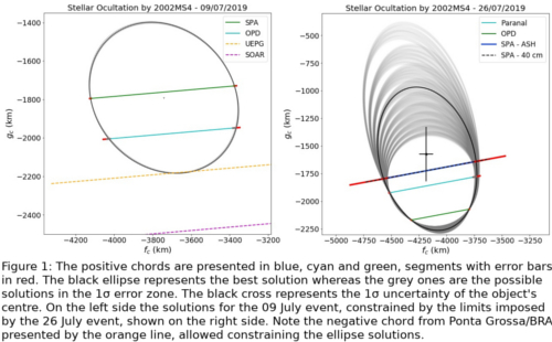
Acknowledgements: F.L.R is thankful for the support of the CAPES scholarship. The following authors acknowledge the respective CNPq grants: F.B-R 309578/2017-5; R.V-M 304544/2017-5, 401903/2016-8; J.I.B.C. 308150/2016-3; M.A 427700/2018-3, 310683/2017-3, 473002/2013-2. This study was financed in part by the Coordenação de Aperfeiçoamento de Pessoal de Nível Superior - Brasil (CAPES) - Finance Code 001 and the National Institute of Science and Technology of the e-Universe project (INCT do e-Universo, CNPq grant 465376/2014-2). G.B-R acknowledges CAPES-FAPERJ/PAPDRJ grant E26/203.173/2016, M.A FAPERJ grant E-26/111.488/2013 and A.R.G-Jr FAPESP grant 2018/11239-8. B.E.M thanks the CAPES/Cofecub-394/2016-05 grant.  P.S-S. acknowledges financial support by the Spanish grant AYA-RTI2018-098657-J-I00 "LEO-SBNAF" (MCIU/AEI/FEDER, UE). We would like to acknowledge financial support from the State Agency for Research of the Spanish MCIU through the “Center of Excellence Severo Ochoa” award for the Instituto de Astrofı́sica de Andalucı́a (SEV-2017-0709) and the financial support by the Spanish grant AYA-2017-84637-R. Part of the results were based on observations taken at the 1.6 m telescope on Pico dos Dias Observatory of the National Laboratory of Astrophysics (LNA/Brazil). Part of this work was carried out within the “Lucky Star" umbrella that agglomerates the efforts of the Paris, Granada and Rio teams. It is funded by the European Research Council under the European Community’s H2020 (2014-2020/ERC Grant Agreement No. 669416). This work has made use of data from the European Space Agency (ESA) mission Gaia (https://www.cosmos.esa.int/gaia), processed by the Gaia Data Processing and Analysis Consortium (DPAC, https://www.cosmos.esa.int/web/gaia/dpac/consortium). Funding for the DPAC has been provided by national institutions, in particular the institutions participating in the Gaia Multilateral Agreement. 

References

Assafin, M. et al. PRAIA - Platform for Reduction of Astronomical Images Automatically. In: Tanga, P.; Thuillot, W. (Ed.). Gaia follow-up network for the solar system objects : Gaia FUN-SSO workshop proceedings, held at IMCCE -Paris Observatory, France, November 29 - December 1, 2010 / edited by Paolo Tanga, William Thuillot.- ISBN 2-910015-63-7, p. 85-88. [S.l.: s.n.], 2011. p. 85–88.

Desmars, J. et al. Orbit determination of trans-Neptunian objects and Centaurs for the prediction of stellar occultations. Astronomy & Astrophysics, v. 584, p. A96, dez. 2015.

Thirouin, A. Study of Trans-Neptunian Objects using photometric techniques and numerical simulations. Dissertation. Editorial de la Universidad de Granada. Spain, 2013.

Trujillo, C. A., Brown, M. E., Minor Planet Electronic Circulars – MPEC  2002-W27. Disponível em: \url{https://minorplanetcenter.net//iau/mpec/K02/K02W27.html}.

Vilenius, E. “TNOs are cool”: a survey of the trans-Neptunian region. VI. Herschel/PACS  observations and thermal modelling of 19 classical Kuiper belt objects. Astronomy & Astrophysics. v. 541, A94, 2012.

How to cite: Rommel, F. L., Braga-Ribas, F., Pereira, C. L., Desmars, J., Santos-Sanz, P., Benedetti-Rossi Rossi, G., Ortiz, J.-L., Morales, N., Jehin, E., Camargo, J. I. B., Assafin, M., Morgado, B. E., Vieira-Martins, R., Sicardy, B., Boufleur, R., Maury, A., Fabrega Polleri, J., Ceravolo, P., Ceravolo, D., Gowe, B., Sfair, R., Santana, T., Mammana, L. A., Lajus, E. F., Colazo, C. A., Spagnotto, J., Gomes-Júnior, A. R., and Winter, O.: Results on stellar occultations by (307261) 2002 MS4, Europlanet Science Congress 2020, online, 21 Sep–9 Oct 2020, EPSC2020-866, https://doi.org/10.5194/epsc2020-866, 2020.

Escalating observations of exo-minor planets and their destroyed remnants both passing through the Solar system and within white dwarf planetary systems motivate an understanding of the orbital history and fate of exo-Kuiper belts and scattered discs.

Here, we explore how the structure of a 40-1000 au annulus of bodies (comets, planetesimals, asteroids) orbiting inside of a Solar system analogue that is itself initially embedded within a stellar cluster environment varies as the star evolves through all of its stellar phases. We attempt this computationally challenging link in four parts: (1) by performing stellar cluster simulations lasting 100 Myr, (2) by making assumptions about the subsequent quiescent 11 Gyr main-sequence evolution, (3) by performing simulations throughout the giant branch phases of evolution, and (4) by making assumptions about the belt's evolution during the white dwarf phase. Throughout these stages, we estimate the planetesimals' gravitational responses to analogues of the four Solar system giant planets, as well as to collisional grinding, Galactic tides, stellar flybys, and stellar radiation.

We find that the imprint of stellar cluster dynamics on the architecture of ≳100 km-sized exo-Kuiper belt planetesimals is retained throughout all phases of stellar evolution unless violent gravitational instabilities are triggered either (1) amongst the giant planets, or (2) due to a close (≪1000 au) stellar flyby. In the absence of these instabilities, these minor planets simply double their semimajor axis while retaining their primordial post-cluster eccentricity and inclination distributions, with implications for metal-polluted white dwarfs and the free-floating planetesimal population.

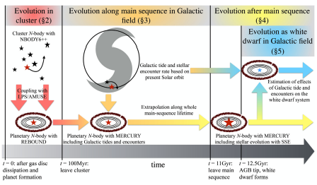
Caption: Cartoon describing how we modelled exo-Kuiper belts through all stages of evolution with different numerical codes and forces.

How to cite: Veras, D., Reichert, K., Flammini Dotti, F., Cai, M., Mustill, A., Shannon, A., McDonald, C., Portegies Zwart, S., Kouwenhoven, M., and Spurzem, R.: Linking the formation and fate of exo-Kuiper belts within Solar system analogues, Europlanet Science Congress 2020, online, 21 Sep–9 Oct 2020, EPSC2020-229, https://doi.org/10.5194/epsc2020-229, 2020.

On 30 August 2019 the amateur Borisov discovered a new comet; after few days it was clear from the characteristics of its orbit (eccentricity > 3 and high hyperbolic excess velocity) that the second interstellar object had been detected and the object received the name of 2I/Borisov.

It appears to be very different from 1I/’Oumuamua and can be considered as the first interstellar comet.

According to the first observations the comet had a nucleus with a radius of few km and a dust coma and tail due to the activity started in June 2019 (Jewitt et al., 2019).

At the beginning of October we submitted the Discretionary Director Time (DDT) proposal to the TNG in order to monitor the comet. Some images have been acquired, in November and December 2019, with the DOLORES instrument in the R filter.

We have applied the dust model described in Fulle et al. (2010), that has been tested on the comet 67P/Churyumov-Gerasimenko and validated with the Rosetta measurements.

According to the results of our dust model and the activity model (Fulle et al., 2020) we derived a water flux from the nucleus of 8x10^-6 kg m^-2 s^-1 and a dust loss rate of 35 and 30 kg s^-1 in November and December 2019 respectively (Cremonese et al., 2020). This slight decrease has been observed around the perihelion on 8 December, few months later the comet fragmented.

In this work we will describe the dust tail observations and the dust model results, even comparing them with the Jupiter family comet 67P.

References:

G.Cremonese, et al., 2020, ApJL, 893, L12

M.Fulle et al., 2010, A&A, 522, A63.

M.Fulle et al., 2020, MNRAS, 493, 4039.

Jewitt et al., 2019, ApJ, 886, L29.

How to cite: Cremonese, G., Fulle, M., Cambianica, P., Munaretto, G., Capria, M. T., La Forgia, F., Lazzarin, M., Migliorini, A., and Boschin, W.: Dust tail observation and modeling of the interstellar comet 2I/Borisov, Europlanet Science Congress 2020, online, 21 Sep–9 Oct 2020, EPSC2020-903, https://doi.org/10.5194/epsc2020-903, 2020.

We present Hubble Space Telescope observations of interstellar comet 2I/Borisov on five occasions between UT 2019 October 12 and 2020 January 29. Our high-resolution images show persistent asymmetry in the dust coma (Figure 1), best explained by a thermal lag on the rotating nucleus, with peak mass loss occurring in the comet nucleus afternoon (Figure 2). In this interpretation, the nucleus rotates with an obliquity of 30 deg (pole direction R.A. = 205 deg and decl. = 52 deg). The subsolar latitude varied from -35 deg (southern solstice) at the time of discovery to 0 deg (equinox) in 2020 January, suggesting that long-term variations in the coma brightness and activity level may be influenced by seasonal effects (Figure 3). Our model shows that newly reported photometric outbursts (Drahus et al. 2020) and the release of a fragment (Jewitt et al. 2020) could result from a seasonal effect, as the northern hemisphere is illuminated for the first time.

Reference: Kim, Y., et al. 2020, ApJL, 895, L34.

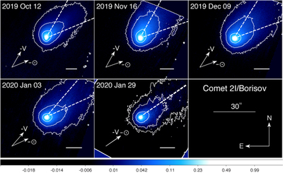
Figure 1: HST images of 2I/Borisov marked with UT dates of observation. Isophotal contours and extended antisolar and negative velocity vectors (dashed lines) are overlaid to highlight an asymmetry in the coma.

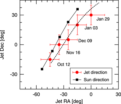
Figure 2: Best-fit solutions for the model jet direction (red circles and dashed line), showing a systematic drift with time from 2019 October to 2020 January. The solutions follow the changing projected direction of the Sun (black squares and solid line), but are offset from it by ~20 deg. The existence of this offset suggests a thermal lag on the rotating nucleus.

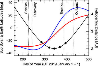
Figure 3: Subsolar (red) and sub-Earth (blue) latitude of 2I/Borisov as a function of time, together with the heliocentric distance (black solid line) on the right axis. We assumed a rotation pole orientation of R.A. = 205 deg and decl. = 52 deg.

How to cite: Kim, Y., Jewitt, D., Agarwal, J., Mutchler, M., Hui, M.-T., and Weaver, H.: Coma Anisotropy and the Rotation Pole of Interstellar Comet 2I/Borisov, Europlanet Science Congress 2020, online, 21 Sep–9 Oct 2020, EPSC2020-955, https://doi.org/10.5194/epsc2020-955, 2020.

We present Hubble Space Telescope observations of a photometric outburst and splitting event in interstellar comet 2I/Borisov.   The outburst, first reported with the comet outbound at 2.8 AU (Drahus et al.~2020), was caused by the expulsion of solid particles having a combined cross-section about 100 sq. km and a mass in 0.1 mm sized particles  2e7 kg.  The latter corresponds to 1e-4 of the mass of the nucleus, taken as a sphere of radius 500 m.  A transient  double nucleus was observed on UT 2020 March 30 (about three weeks after the outburst), having a cross-section 0.6 sq. km and corresponding dust mass 1e5 kg.  The secondary was absent in images taken on and before March 28, and in images taken on and after April 03.  The unexpectedly delayed appearance and rapid disappearance of the secondary are consistent with an origin through rotational bursting of one or more large (meter-sized) boulders under the action of outgassing torques, following their ejection from the main nucleus.  Overall, our observations  reveal that the outburst and splitting of the nucleus are minor events involving a negligible fraction of the total mass: 2I/Borisov will survive its passage through the planetary region largely unscathed.

Journal: The Astrophysical Journal Letters, Volume 896, Issue 2, id.L39

How to cite: Jewitt, D., Kim, Y., Mutchler, M., Weaver, H., Agarwal, J., and Hui, M.-T.: Outburst and Splitting of Interstellar Comet 2I/Borisov, Europlanet Science Congress 2020, online, 21 Sep–9 Oct 2020, EPSC2020-964, https://doi.org/10.5194/epsc2020-964, 2020.

We present the first optical observations taken to characterize the near-Earth object 138175 (2000 EE104).  This body is associated with Interplanetary Field Enhancements (IFEs), thought to be caused by interactions between the solar wind magnetic field and solid material trailing in the orbit of the parent body.  Based on optical photometry, the radius (in meters) and mass (in kilograms) of an equal-area sphere are found to be  250(0.1/p)^{1/2} and  1e11(0.1/p)^{3/2}, respectively, where p is the red geometric albedo and density 1500 kg/m3 is assumed.  The measured colors are intermediate between those of C-type (primitive) and S-type (metamorphosed) asteroids but, with correction for the likely effects of phase-reddening, are more consistent with a C-type classification than with S-type. No evidence for co-moving companions larger than 40(0.1/p) meter in radius is found, and no dust particle trail is detected, setting a limit to the trail optical depth < 2e-9.  Consideration of the size distribution  produced by impact pulverization  makes it difficult to generate the  mass of nanodust (minimum 1e5 kg to 1e6 kg) required to account for IFEs, unless the size distribution is unusually steep.  While the new optical data do not definitively refute the hypothesis that boulder pulverization is the source of IFEs, neither do they provide any support for it.

Journal: Planetary Science Journal, submitted

How to cite: Jewitt, D.: 138175 (2000 EE104) and the Source of Interplanetary Field Enhancements, Europlanet Science Congress 2020, online, 21 Sep–9 Oct 2020, EPSC2020-965, https://doi.org/10.5194/epsc2020-965, 2020.

We will present the results of coordinated observations of 2I/Borisov with the Neil Gehrels-Swift observatory (Swift) and Hubble Space Telescope (HST), which allowed us to provide the first glimpse into the ice content and chemical composition of the protoplanetary disk of another star. Comets are condensed samples of the gas, ice and dust that were in a star’s protoplanetary disk during the formation of its planets, and inform our understanding on how chemical compositions and abundances vary with distance from the central star. Their orbital migration distributes volatiles [1], organic material and prebiotic chemicals around their host system [2]. In our Solar System, hundreds of comets have been observed remotely, and a few have been studied up close by space missions [3].  Similarly, interstellar comets offer a glimpse into the building blocks, formation, and evolution of other planetary systems.  However, knowledge of extrasolar comets has been limited to what could be gleaned from distant, unresolved observations of cometary regions around other stars. 2I/Borisov, discovered in Aug. 2019, is the first notably active interstellar comet discovered in our Solar System [4].

We used the UltraViolet Optical Telescope (UVOT) of Swift to determine 2I/Borisov’s water production rates and dust content surrounding the nucleus at six epochs spaced before and after perihelion on Dec. 8.55, 2019 UTC (-2.56AU to 2.54AU) [5]. Water production rates increased steadily before perihelion at a rate of increase quicker than that of most dynamically new comets but slower than most Jupiter-family comets. After perihelion, the water production rate decreased much more rapidly than that of all previously observed comets. We used a sublimation model to constrain the active area and minimum radius of the nucleus, and found that a significant fraction of the surface of Borisov is active. 

We also used Cosmic Origins Spectrograph (COS) on the HST during four epochs around the perihelion and clearly detected the emissions of several bands of the CO Fourth Positive system, which we used to derive CO production rates [6]. Comparing these with the water production rates determined by Swift, we found that after perihelion, the coma of 2I/Borisov contains substantially more CO than H2O gas. Our abundances were more than three times higher than previously measured for any comet in the inner (<2.5 au) Solar System [3]. The derived high abundance ratio of CO/H2O and high elemental abundance of carbon relative to oxygen firmly sets 2I/Borisov apart from solar system comets, and suggest that the physical and chemical environment were Borisov was formed are substantially different from those in our solar system [6, 7] .

Fig. 1 Volatile production rates as a function of time relative to perihelion [6]. The production rates of CO measured with HST/COS (this work) and the water production rate measured by Swift (based on OH, open circles; 5) and the Very Large Telescope/UVES (based on OH, 8), and at the Apache Point Observatory (based on [OI], 9). Arrows indicate 3-σ upper limits, and error bars indicate 1-σ stochastic uncertainties. The grey line indicates the temporal trend of water production rates used to derive the elemental composition.

References:

[1] Cleeves, L. I. et al. The ancient heritage of water ice in the solar system. Science 345, 1590–1593 (2014).

[2] Rubin, M., Bekaert, D. V., Broadley, M. W., Drozdovskaya, M. N., and Wampfler, S. F. Volatile Species in Comet 67P/Churyumov-Gerasimenko: Investigating the Link from the ISM to the Terrestrial Planets. ACS Publ. 3, 1792–1811 (2019).

[3] Bockelée-Morvan, D. & Biver, N. The composition of cometary ices. Phil. Trans. R. Soc. A 375, 20160252–11 (2017).

[4] Guzik, P. et al. Initial characterization of interstellar comet 2I/Borisov. Nature Astron. 4, 53 - 57 (2019).

[5] Xing, Z., Bodewits, D., Noonan, J., and Bannister, M. T. Water Production Rates and Activity of Interstellar Comet 2I/Borisov. Astrophys. J. 893, L48 (2020).

[6] Bodewits, D., Noonan, J. et al. The carbon monoxide-rich interstellar comet 2I/Borisov. Nature Astron. doi:10.1038/s41550-020-1095-2 (2020).

[7] Cordiner, M.A., Milam, S.N., Biver, N. et al. Unusually high CO abundance of the first active interstellar comet. Nature doi:Astron.https://doi.org/10.1038/s41550-020-1087-2 (2020).

[8] Lupu, R. E., Feldman, P. D., Weaver, H. A. & Tozzi, G.-P. The Fourth Positive System of Carbon Monoxide in the Hubble Space Telescope Spectra of Comets. Astrophys. J. 670, 1473-1484 (2007).

[9] McKay, A. J., Cochran, A. L., Dello Russo, N. & DiSanti, M. A. Detection of a Water Tracer in Interstellar Comet 2I/Borisov. Astrophys. J. 889, L10 (2020)

How to cite: Xing, Z.-X., Bodewits, D., Noonan, J. W., Feldman, P. D., Bannister, M. T., Farnocchia, D., Harris, W. M., Li, J.-Y., Mandt, K. E., and Parker, J. Wm.: Activities and origins of interstellar comet 2I/Borisov, Europlanet Science Congress 2020, online, 21 Sep–9 Oct 2020, EPSC2020-993, https://doi.org/10.5194/epsc2020-993, 2020.

(596) Scheila was observed to have an active appearance as a result of impact event in late 2010. In additional the coma feature, the shape of light curve had been found the difference probably fresh material or surface properties changed around the impact site. In this study, we present the results of our monitoring observations obtained in 2014 and 2019-2020. The mean values of the color indices (B−V = (0.75 ± 0.08)^m, V−R = (0.45 ± 0.04)^m, and R−I = (0.44 ± 0.09)^m) agree well with the values for asteroids of the D-types. The rotation period of the asteroid estimated from photometric observations in 2014 is 15.8 ± 0.1 h. The shape of the light curve is similar as that found after impact event. Furthermore, we did not find any rotational color variability in B-V, V-R and R-I diagrams, meaning the observed surface in this observing period of 2019-2020 is homogeneous.

How to cite: Lin, Z.-Y. and Hsu, C.-Y.: Photometric results of the long-term monitoring of the active asteroid (596) Scheila, Europlanet Science Congress 2020, online, 21 Sep–9 Oct 2020, EPSC2020-1034, https://doi.org/10.5194/epsc2020-1034, 2020.

Abstract

We studied the dust activity of comet 67P/Churyumov-Gerasimenko (67P), by relating the detections of the Rosetta/ GIADA and MIDAS instruments, obtaining a correlation between flux of ejected mm- and μm-sized dust.

The ESA/Rosetta mission orbited the 67P comet for two years, escorting it through perihelion, occurred on 13th August 2015.

The mission configuration is still permitting a thorough characterization of cometary activity, even 4 years from the end of the mission.

In particular, the 67P’s dust ejection has been detected in different stages of the comet’s orbit by both remote observations (e.g., the OSIRIS camera and the VIRTIS imaging spectrometer) and in-situ measurements performed by detectors as GIADA, MIDAS and COSIMA.

This work merges data from the GIADA (Grain Impact Analyser and Dust Accumulator) [1] dust detector and the MIDAS (Micro-Imaging Dust Analysis System) [2] atomic force microscope. The two instruments detected dust different in size (mm-sized vs μm-sized) and complementary dust properties (porosity and mass vs physical properties and 3D structure). The GIADA and MIDAS data fusion could allow to relate ejection of smaller and larger dust particles as well as to monitor variations of dust properties during Churyumov-Gerasimenko’s orbit and to link them to the morphology of ejecting surface regions.

2.1 The GIADA dataset

The GIADA instrument consists of three subsystems: Grain Detection System (GDS), Impact Sensor (IS) and Quartz Crystal Microbalances (QCM). The first two subsystems measured velocity of fluffy particles and momentum of compact (mm-sized) particles, respectively, whereas the QCM measured the cumulative mass of nm-sized dust [3].

To compare GIADA and MIDAS dataset, we considered only the IS data, because MIDAS mostly detected individual compact particles. In particular, we considered only the IS detections acquired in the periods when MIDAS detected dust particles (see next subsection).

[4] developed a procedure to trace back the motion of dust particles detected by GIADA in the coma down to the nucleus surface. This allowed the retrieval of the geomorphological region ejecting each dust particle and the association of dust and surface properties. These results are intended to be extended to the GIADA-MIDAS data fusion to relate dust physical properties and surface morphology.

2.2 The MIDAS dataset

MIDAS collected micron-sized dust particles on several targets, each working in a defined period. Cometary dust was detected on four MIDAS targets: Target 10, Target 12 and Target 14 collected dust in three periods before perihelion (September-November 2014, December2014-February 2015 and February-March 2015, respectively), whereas the dust collected on Target 13 was released in an outburst on 19^th February 2016 (after perihelion).

Except one case of a fluffy agglomerate [5], all the particles detected by MIDAS are compact.

3.1 mm- vs μm- sized dust flux

Our first step was to compare the millimetric and micrometric dust flux measured by GIADA-IS and MIDAS, respectively.

For each period corresponding to the collection time of a MIDAS target, we retrieved the number of particles detected by the two instruments, normalized it to the period duration (in days) and to the spacecraft-comet distance (in km). The MIDAS flux required an additional normalization, taking into account the scanned area on the respective target (not constant among targets).

The comparison of dust fluxes measured by GIADA and MIDAS is shown in Figure 1.

Figure 1. Dust fluxes measured by MIDAS and GIADA. Each asterisk corresponds to a MIDAS target, i.e., to a defined orbit period. The red asterisk corresponds to MIDAS Target 14 (which detected dust between February and March 2015).

The flux logarithms are linearly related, suggesting a strong correlation between ejection of large (mm-sized) and small (mm-sized) compact dust agglomerates.

The flux corresponding to the MIDAS Target 14 period (February/March 2015), highlighted in red in Figure 1, is slightly outside this linear trend, with GIADA (MIDAS) detecting more (less) particles than expected from the linear trend identified by the other three periods. This can be ascribed to the occurrence of an outburst (detected by GIADA but not by MIDAS) in a moment when the spacecraft had the largest distance to the comet among all herein considered periods. As smaller particles are stronger deviated from their initially radial trajectory than larger ones (due to  the more important role of solar pressure force with respect to nucleus gravity [6]), it is reasonable that fewer small than large particles arrived at the spacecraft position. However, this result needs further refinement regarding a possible falsification of MIDAS particle size distribution caused by particle fragmentation upon collection. Our next steps are to discern parent particles and fragments in the MIDAS data set and to update the relation shown in Figure 1. This will be done by analyzing the spatial distribution of dust particles on the MIDAS targets, by comparing  MIDAS’ dust size distribution to that expected during nominal activity [7] and during outbursts [8] and by taking into account the largest dust size expected to be ejected depending on the nucleus surface temperature [9].

3.2 Dust vs surface properties

By applying the traceback algorithm developed by [4], we obtained that in certain periods dust is mostly ejected from rough or from smooth terrains. Therefore, we can relate properties of particles stemming from different locations at the comet to cometary surface morphology. In addition, dust ejected during outbursts may probe deeper layers of the comet, allowing us to discern dust properties at different depths.

Acknowledgements

This research was supported by the Italian Space Agency (ASI) within the ASI-INAF agreement I/032/05/0, by the Austrian Science Fund FWF P 28100-N36, and by the International Space Science Institute (ISSI) through the ISSI International Team “Characterization of cometary activity of 67P/Churyumov-Gerasimenko comet”.

References

[1] Della Corte, V. et al. (2014) JAI 1350011-1350022; [2] Bentley, M.S. et al. (2016), Acta Astronautica 125; [3] Della Corte, V. et al. (2019), A&A 630, A25, 13 pp.; [4] Longobardo, A. et al. (2020), MNRAS 496, 1, 125-137; [5] Mannel, T. et al. (2016), MNRAS 462; [6] Zakharov, V.V. et al. (2018), Icarus, 312, 121-127; [7] Rinaldi, G. et al. (2016), MNRAS 462, 1, S547-S561; [8] Bockelée-Morvan, D. et al. (2017), MNRAS, 469 2, S443-S458; [9] Fulle, M. et al. (2020), MNRAS, 493, 4039-4044.

How to cite: Longobardo, A., Mannel, T., Rinaldi, G., Fulle, M., Rotundi, A., Della Corte, V., Ivanovski, S., and Formisano, M.: Merging data from Rosetta GIADA and MIDAS dust detectors to characterize 67P’s activity, Europlanet Science Congress 2020, online, 21 Sep–9 Oct 2020, EPSC2020-1044, https://doi.org/10.5194/epsc2020-1044, 2020.

The fine-structure detail of several comet dust tails is analysed from amateur and professional comet images using the Finson-Probstein mdoel. Given the date and time of the image taken, the comet’s position in the sky is calculated using an open source algorithm [1] and the comet’s dust tail is simulated for that position and time. This modeled dust tail structure is then projected and overlaid onto the comet image to directly compare and identify similarities and discrepancies between the model and the image. Using the novel analysis method of mapping the image to a dust grain beta against ejection time plot [2], tail structures can be more easily identified and analysed. This also allows for the tracking of tail structure over time, as images of a single comet from different times and observatories can be mapped onto the same plot. This method compensates for the difficulties of investigating tail structures in images as the comet moves across the image and as viewing geometry changes over time.      

This is a continuation of the work done previously on Comet C/2006 P1 (McNaught), which ultimately led to the observation of the formation processes of new fine-scale structure features in the comet’s dust tail [2]. This model is now applied to several other comets, including the recent Comet ATLAS (C/2019 Y4), to map their tail structures and to highlight this model’s utility in comet dust tail analysis.

Finally, this work will be put into context as the first step in the development of an automated analysis method for cometary dust and ion tails. This automated method is in preparation for the upcoming opening of the Vera Rubin Observatory (LSST), and aims to automatically identify comet tail structures from the Observatory’s stream of comet images. The robustness of this analysis suite enables it to also be implemented on amateur comet images, making use of the abundant and valuable data from amateur astronomers.

[1] Lang, Dustin, David W. Hogg, Keir Mierle, Michael Blanton, and Sam Roweis. 2010. "ASTROMETRY.NET: BLIND ASTROMETRIC CALIBRATION OF ARBITRARY ASTRONOMICAL IMAGES". The Astronomical Journal 139 (5): 1782-1800. doi:10.1088/0004-6256/139/5/1782.

[2] Price, Oliver, Geraint H. Jones, Jeff Morrill, Mathew Owens, Karl Battams, Huw Morgan, Miloslav Drückmuller, and Sebastian Deiries. 2019. "Fine-Scale Structure In Cometary Dust Tails I: Analysis Of Striae In Comet C/2006 P1 (Mcnaught) Through Temporal Mapping". Icarus 319: 540-557. doi:10.1016/j.icarus.2018.09.013.

How to cite: Afghan, Q., H. Jones, G., and Price, O.: Comet Dust Tail Analysis using the Finson-Probstein Model, Europlanet Science Congress 2020, online, 21 Sep–9 Oct 2020, EPSC2020-1068, https://doi.org/10.5194/epsc2020-1068, 2020.

Abstract:

 A search for the detection of vibrationally excited Polycyclic Aromatic Hydrocarbons on a sample of comets observed by Infrared Spectrometer (IRS) onboard Spitzer Space Telescope was initiated. A continuum was subtracted from the observed spectra to clearly delineate the presence of PAH emission bands in the wavelength 5.4 to 14 um. Our analysis showed the presence of Polycyclic Aromatic Hydrocarbons (PAHs) in the mid-infrared spectra of four comets.

 The evolution of organic molecules on their journey from molecular clouds to the early solar system is not well understood. Comets are considered to be primitive bodies formed during the formation of solar system that contain agglomerate of frozen gases, ices and rocky debris. It is believed that comets are made of unaltered interstellar materials and preserve the early stages of solar nebula [1]. Polycyclic Aromatic Hydrocarbons (PAH) molecules consisting of fused benzene rings with a wide spread presence in the ISM of our own and external galaxies are believed to be frozen in comets. The infrared emission bands at 3.3, 6.2, 7.7, 8.6 and 11.2 um are attributed to the C-H stretching and bending vibrations and C=C stretching modes of PAH molecules [2]. Traditionally, Ultraviolet fluorescent spectra of PAH at 347, 356 and 364 nm was used for its identification [3].

 The public archival spectroscopic data on a sample of comets observed by Infrared Spectrometer (IRS) onboard Spitzer Space Telescope covering the mid-IR region between 5.3 and 38 um [4] was used for the present analysis. The IRS stare observations using the Short-Low module was mostly used for the present study. The mid-infrared spectra was extracted from the Basic Calibrated Spectra (BCDs) using Spectroscopic Modeling Analysis and Reduction Tool (SMART) [5]. 

The extracted mid-infrared spectra in the wavelength range 5.3 and 14 um was subjected to continuum subtraction for clearly delineating the PAH bands. The continuum was defined by the pivotal on the spectra that are fitted by a third order polynomial for the entire region (see top panel of Fig 1). The bottom panel in Figure 1 shows the continuum subtracted spectra.

The mid-infrared spectra of four comets in our sample showed faint emission from PAH bands. The comets  Schwassmann-Wachmann-3, Neat (C/2001 Q4),  46P/Wirtanen and McNaught (C2006 P1) showed vibrationally excited PAH bands at  6.2, 7.7, 8.6 and 11.2 um.

The heliocentric distance (r_h) of Schwassmann-Wachmann-3 was 1.47 AU and the distance between the comet and Spitzer (∆_s) was 0.78 AU during the observation. For Neat (C/2001 Q4) r_h  was 4.59 AU and ∆_s  was 4.36 AU. For 46P/Wirtanen r_h  was 2.08 AU and ∆_s was 1.8 AU. The r_h  for McNaught (C2006 P1) is 3.6 AU and ∆_s was 2.2 AU. The position of these comets that approached Sun during its observation well suited for the detection of PAH at mid-infrared wavelengths. In addition, all sources showed silicate emissions at 9.8 um. Thus a mixed chemistry minerology was observed. The mid-infrared spectra of Schwassmann-Wachmann-3 also showed a peak at 9.2 um due to the aliphatic hydrocarbons. Lisse et al [6] found PAH emission bands in the deep impact ejecta of comet Tempel 1 using Spitzer. Takafumi Ootsubo et al [7] detected PAH and crystalline silicates in comet 21P/G-Z using the Cooled Mid-infrared Camera and Spectrometer (COMICS) on the 8.2 m Subaru Telescope.  They propose that comets with crystalline silicate and PAH features may be formed in the circumplanetary disk around a gas giant planet like Jupiter or Saturn, owing to the favourable temperature conditions for the existance of the dust grain. Our results with spectral signatures of both PAH and silicate features observed in the comets and the possible pathways for incorporating them from the ISM will be discussed.

References:

[1] Greenberg, J.M. 1982, in Comets, ed. L.L. Wilkening (Tuscon: Univ. of Arizona Press), 131

[2] Tielens, A.G,G.M., 2005, The Physics and Chemistry of the Interstellar Medium, Cambridge University press, p 215

[3] Moreels, G., Clairemidi, J., Hermine, P., Brechignac, P., & Rousselott, P. 1994, A&A, 282, 643

[4] Houck et al. In J. C. Mather, editor, Optical, Infrared, and Millimeter Space Telescopes, volume 5487 of Proc. SPIE, pages 62–76, October 2004

[5] Higdon, S. J. U. et al. 2004, PASP, 116, 975

[6] Lisse, C.M., et al. 2006, Science, 313, 635

[7] Takafumi et al., 2020, Icarus,338, 113450

How to cite: Raman V, V., Roy, A., Sivaraman, B., Ganesh, S., and Mason, N.: Tentative detection of vibrationally excited Polycyclic Aromatic Hydrocarbons in Comets, Europlanet Science Congress 2020, online, 21 Sep–9 Oct 2020, EPSC2020-1072, https://doi.org/10.5194/epsc2020-1072, 2020.