TP8 | Atmospheres and Exospheres of Terrestrial Bodies

TP8

Atmospheres and Exospheres of Terrestrial Bodies
Co-organized by MITM/EXOA
Conveners: Gabriella Gilli, Francisco González-Galindo | Co-conveners: Panayotis Lavvas, Giuliano Liuzzi, Yann Leseigneur, Joanna Egan, Tanguy Bertrand
Orals THU1
| Thu, 10 Sep, 08:30–10:00 (CEST)|Room Neptune (Spinoza Foyer)
Orals THU2
| Thu, 10 Sep, 11:00–12:30 (CEST)|Room Neptune (Spinoza Foyer)
Orals THU3
| Thu, 10 Sep, 14:00–15:30 (CEST)|Room Neptune (Spinoza Foyer)
Orals THU4
| Thu, 10 Sep, 16:00–17:30 (CEST)|Room Neptune (Spinoza Foyer)
Posters TUE-POS
| Attendance Tue, 08 Sep, 18:00–19:30 (CEST) | Display Tue, 08 Sep, 08:30–19:30|Foyer 2, F2.22–43
Thu, 08:30
Thu, 11:00
Thu, 14:00
Thu, 16:00
Tue, 18:00
Understanding why planetary atmospheres look the way they do today - and reconstructing the evolutionary pathways that brought them to their present states - is one of the most compelling questions in modern planetary science. This session adopts a comparative planetology perspective, bridging solar system bodies and exoplanet populations through the lens of atmospheric evolution, investigated through observations, modelling, and mission-driven science.
Space missions have delivered a wealth of observations of the atmospheres and aeronomy of rocky planets and moons, from the lower atmosphere to regions interacting directly with the solar wind. With recent advances and forthcoming missions, planetary atmospheric science is entering a particularly active phase. This session invites contributions on the physical and chemical processes shaping the lower, middle, and upper atmospheres of terrestrial bodies in the Solar System and beyond, including atmospheric chemistry, energetics, dynamics, electrodynamics, atmospheric escape, surface–atmosphere interactions, and coupling with the space environment. We welcome studies based on spacecrafts (e.g., Messenger, BepiColombo, Venus Express, Akatsuki, EnVision, Davinci, Mars Express, MRO, TGO, EMM, MAVEN, MMX, among others), ground-based observations, numerical modelling, and laboratory experiments.
We welcome contributions addressing the long-term evolution of atmospheres across all planetary types. In the inner solar system, Venus and Mars stand as striking cases of evolutionary divergence from Earth. In view of upcoming ESA and NASA Venus missions, contributions addressing current understanding, open questions, and preparatory studies of the Venus atmosphere and its long-term history are particularly encouraged, from photochemistry and cloud dynamics to the transformative science expected from ESA's EnVision (and its VenSpec suite) and DAVINCI.
In the outer solar system, Titan's organic-rich and seasonally evolving atmosphere offers a unique window into photochemical complexity and long-term change, with new observational and modelling efforts building on the Cassini legacy. The gas and ice giants - characterized with unprecedented detail by JWST, Juno, and the forthcoming JUICE mission - further enrich this comparative picture; ice giant atmospheres in particular represent a frontier for solar system science and an archetype for the most abundant planetary class in the galaxy, with the scientific case for a Uranus mission gaining momentum under NASA's Decadal Survey and ESA's Voyage 2050 framework.
Finally, broader comparative studies linking solar system atmospheric structure and chemistry to the growing population of exoplanets accessible to spectroscopic characterization are warmly welcomed. This includes contributions on atmospheric escape and its demographic imprints on exoplanet populations - from the radius valley and the Neptune desert to observations of young systems caught in the act of losing their envelopes. Both observational and modelling contributions are welcome, as well as cross-disciplinary studies connecting solar system and exoplanet atmospheric science through laboratory measurements, modeling and/or observations.
The session will include solicited and contributed oral presentations, as well as posters.

Orals THU1: Thu, 10 Sep, 08:30–10:00 | Room Neptune (Spinoza Foyer)

Mars atmospheric composition
08:30–08:33
08:33–08:48
|
EPSC2026-170
|
solicited
|
On-site presentation
Jean-Claude Gérard and Lauriane Soret

The first detection of aurora in the Mars night sky was made in 2005 with the SPICAM ultraviolet spectrometer on board Mars Express. It revealed the presence of emissions from CO, CO2+ and O, concentrated in regions of strong open magnetic field lines in the southern hemisphere. Further ultraviolet observations with the IUVS instrument on board MAVEN and EMUS on the Emirates Mars missions measured the N2 Vegard-Kaplan bands, the OI 130.4 and 135.6 nm and the CI 156.1 and 165.7 nm emissions.

All space-borne instruments so far were only able to observe in the ultraviolet. Yet, laboratory simulations of the aurora at low CO2 pressure have shown the presence of the CO2+ Fox-Duffendack-Barker (FDB) emission between 300 and 500 nm with 7% of the intensity in the blue. The oxygen green and red lines were not observed. More recently, the green line at 557.7 nm has been unambiguously measured from the Martian surface with the Supercam spectrometer covering the 535-853 nm range and the Mastcam-Z imaging camera on the Perseverance rover during Solar Energetic Particle Events. It is mainly excited by collisions of energetic electrons with ambient CO2. ESA’s M-MATISSE mission will carry the Mars Aurora and dust Camera (M-AC) equipped with a green line (557.7 nm) and a FDB channel (367.0-393.2 nm).

In contrast, the Martian ultraviolet nightglow is characterised by the presence of the nitric oxide δ and ϒ bands between 180 and 300 nm discovered with Mars Express-SPICAM. It is caused by radiative recombination of O and N atoms created on the day side. Additional emissions in the near infrared and visible ranges result from three-body recombination of O atoms in the winter polar regions. The visible contribution corresponds to the O2 c 1u - X 3g Herzberg II band system extending from 300 to 600 nm. It is expected to be bright enough to be observable with the naked eye in the winter polar regions from Mars orbit and from the surface.

In this presentation, we will combine observed spectral measurements with Monte Carlo modelling of the excitation rates to define the colours and the visibility of the nightside emissions.

How to cite: Gérard, J.-C. and Soret, L.: The colours of the Mars night sky: when  aurora and nightglow illuminate the atmosphere, Europlanet Science Congress 2026, The Hague, The Netherlands, 7–11 Sep 2026, EPSC2026-170, https://doi.org/10.5194/epsc2026-170, 2026.

08:48–09:00
|
EPSC2026-1146
|
ECP
|
On-site presentation
zachary Flimon, Lauriane Soret, Jean-Claude Gérard, and Benoit Hubert and the NOMAD team

O2 and NO nightglow emission on Mars from NOMAD UVIS


Nightglow observations on Mars provide important insights into the chemical and dynamical processes of the Martian atmosphere. The first visible observations of nitric oxide (NO) nightglow were reported by (Bertaux et al. 2005) using the SPectroscopy for the Investigation of the Characteristics of the Atmosphere of Mars (SPICAM) instrument aboard Mars Express. Additional NO observations were later obtained with the Imaging Ultraviolet Spectrograph (IUVS) instrument aboard Mars Atmosphere and Volatile Evolution (MAVEN). These visible emissions originate from the recombination of oxygen and nitrogen atoms produced on the dayside through the photodissociation of CO₂ and N₂ and subsequently transported to the nightside by atmospheric circulation. The resulting NO nightglow emissions provide valuable information on the product of the densities of atomic oxygen and nitrogen in the upper atmosphere. In the visible it is also possible to observe the O2 Herzberg II emission, this emission was first observed by (Gérard et al. 2023; Soret et al. 2024) using the UVIS channel of the Nadir and Occultation for Mars Discovery (NOMAD) instrument.

The NOMAD spectrometer aboard the ExoMars Trace Gas Orbiter (Vandaele et al. 2018) began science operations in April 2018. In this work, we investigate limb observations from the UV‐visible (UVIS) channel of NOMAD ( Vandaele et al. 2015). Covering a wavelength range from 200 to 650 nm, UVIS enables simultaneous observation of NO δ and γ bands between 205 and 270 nm and O₂ Herzberg II emissions between 400 and 600 nm. Using dedicated observation modes, this study explores the UVIS dataset with the objective of deriving atmospheric parameters from these nightglow emissions.

The methodology consists first of retrieving the emission intensities from UVIS limb spectra. We apply the same approach as described by (Soret et al. 2024), by fitting reference spectra derived from previous missions (Venus for O2 and MAVEN for NO) to compute the total intensity at each altitude due to the nightglow emission. From the resulting vertical intensity profiles, Chapman functions are fitted to derive the volume emission rates. Using these emission rates and the corresponding chemical relationships, we retrieve the densities of atomic oxygen and nitrogen.

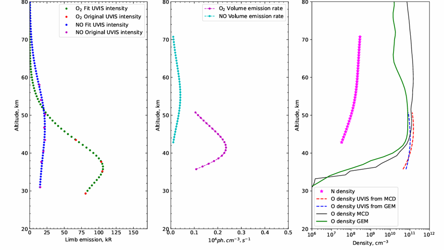
The altitude probed are between 20 to 80 km with the peak emission of NO on average 20 km above the emission of O2. All observations are in the polar regions and the limited number of limb profiles (around 50 from MY35 to MY 38) limit the interpretation for seasonality. An example showing the different vertical profiles can be found in Figure 1. Currently the density of N is not included in the model but new simulations should be provided allowing the comparison.

This work provides a climatology of NO and O₂ nightglow emissions observed simultaneously by NOMAD-UVIS, together with the corresponding atomic oxygen and nitrogen densities at coincident altitudes whenever possible. Finally, the retrieved densities are compared with predictions from global climate models, including GEM (Neary and Daerden 2018) and PCM (Millour et al. 2018). Overall, the modeled density profiles show good agreement with the observations.

Figure 1: Vertical profiles for NO and O2 emissions on the first panel, the middle panel represents the volume emission rate and the last panel the O and N densities. In the last panel the densities for O are computed using the temperature from GEM or the MCD. In this case, the value for the O densities at the peak are similar between the models and the observations.


Bertaux, Jean-Loup, François Leblanc, Séverine Perrier, et al. 2005. “Nightglow in the Upper Atmosphere of Mars and Implications for Atmospheric Transport.” Science 307 (5709): 566–69. https://doi.org/10.1126/science.1106957.

Gérard, J. C., L. Soret, I. R. Thomas, et al. 2023. “Observation of the Mars O2 Visible Nightglow by the NOMAD Spectrometer Onboard the Trace Gas Orbiter.” Nature Astronomy 8 (1): 77–81. https://doi.org/10.1038/s41550-023-02104-8.

Millour, E., F. Forget, A. Spiga, et al. 2018. THE MARS CLIMATE DATABASE (VERSION 5.3).

Neary, L., and F. Daerden. 2018. “The GEM-Mars General Circulation Model for Mars: Description and Evaluation.” Icarus 300 (January): 458–76. https://doi.org/10.1016/j.icarus.2017.09.028.

Soret, L., F. González‐Galindo, J. ‐C. Gérard, et al. 2024. “Ultraviolet NO and Visible O2 Nightglow in the Mars Southern Winter Polar Region: Statistical Study and Model Comparison.” Journal of Geophysical Research: Planets 129 (12): e2024JE008620. https://doi.org/10.1029/2024JE008620.

Vandaele, A. C., J. J. Lopez-Moreno, M. R. Patel, et al. 2018. “NOMAD, an Integrated Suite of Three Spectrometers for the ExoMars Trace Gas Mission: Technical Description, Science Objectives and Expected Performance.” Space Science Reviews 214 (5): 80. https://doi.org/10.1007/s11214-018-0517-2.

Vandaele, Ann C., Yannick Willame, Cédric Depiesse, et al. 2015. “Optical and Radiometric Models of the NOMAD Instrument Part I: The UVIS Channel.” Optics Express 23 (23): 30028. https://doi.org/10.1364/OE.23.030028.

How to cite: Flimon, Z., Soret, L., Gérard, J.-C., and Hubert, B. and the NOMAD team: O2 and NO nightglow emission on Mars from NOMAD UVIS, Europlanet Science Congress 2026, The Hague, The Netherlands, 7–11 Sep 2026, EPSC2026-1146, https://doi.org/10.5194/epsc2026-1146, 2026.

09:00–09:12
|
EPSC2026-312
|
On-site presentation
Timothy McConnochie and the Co-authors

The Curiosity rover’s ChemCam instrument suite and the Perseverance rover’s SuperCam instrument suite have been conducting routine passive UV-to-near-IR spectroscopy of the Martian sky since, respectively, 2013 and 2021. From these “passive sky” observations we retrieve column abundances of trace gases O2 and H2O, as well as aerosol properties, using a combination of grid-search based and Nelder Mead (also known as “downhill simplex”) optimization, and discrete-ordinates multiple-scattering radiative transfer models with correlated-k-based gas absorption. Ratios of high-elevation angle to low-elevation angle sky pointings are used to divide out most instrumental uncertainties and make weak spectral features detectable.

The latest passive sky aerosol results are described by Stcherbinine et al. (this meeting; EGU 2026). Here, we focus on the latest trace gas measurement results.

The passive sky trace gas results are important for testing hypotheses about the unexplained variability of O2 abundances relative to argon and other inert trace gases (Trainer et al., 2019; Lo et al., 2024). They also help constrain surface-atmosphere exchange of water vapor (e.g. Savijärvi et al., 2019). Furthermore, the rapid (roughly every 14 – 21 days in most years) sampling of O2 and water vapor abundances provided by passive sky combined with similar sampling of Ar with APXS on Curiosity (VanBommel et al. 2018, 2024) provides evidence for close correlation of water vapor with the O2/Ar variability in northern summer (McConnochie et al., 2024).

The possibility of such a correlation was first suggested by the results of the Viking Gas Exchange experiments, which showed release of O2 from a soil sample in response to adding water vapor (Klein, 1978; Oyama & Berdahl, 1977), and by the fact that a surface/subsurface reservoir of O atoms appears to be required because atmospheric reservoirs of O atoms are too small to supply the observed magnitude of O2 variability (Trainer et al., 2019). Soil oxychlorines have been proposed (Trainer et al., 2019; Lo et al., 2024) as the soil reservoir for O atoms, as were superoxide ions in the context of the Viking Gas Exchange experiments (Yen et al., 2000), but specific reactions with the necessary rates to explain the apparent seasonal cycle of O2 into and out of the soil have not been identified.

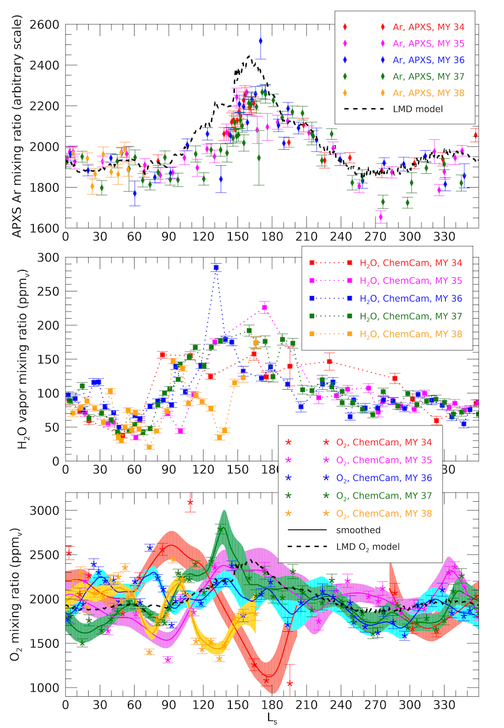
The details and timing of the O2-to-water-vapor correlation, combined with the information about the effects of the global circulation on all trace gases that is provided by Ar measurements, could potentially constrain the mechanisms and predominant locations for the apparent O2 cycle. However as shown in Figure 1, the apparent O2 cycle has substantial interannual variability despite only modest interannual variability in Ar and H2O. We have therefore been working to both extend the passive sky and APXS argon data sets and to improve data analysis methods. New developments in work include initial O2 measurements from Perseverance-SuperCam, explicit modeling of stray light effects on gas absorption lines for both SuperCam and ChemCam, and more accurate detector background subtraction and outlier rejection for ChemCam. Even in their current form, however, the ChemCam O2 measurements show statistically significant variability relative to argon, just as the SAM O2 measurements in Trainer et al. (2019) do. They also show, as detailed in Figure 1, significant interannual variability, especially around northern hemisphere summer solstice, and a tendency for the timing of the northern spring-summer seasonal increase in O2/Ar to be correlated with that of water vapor.

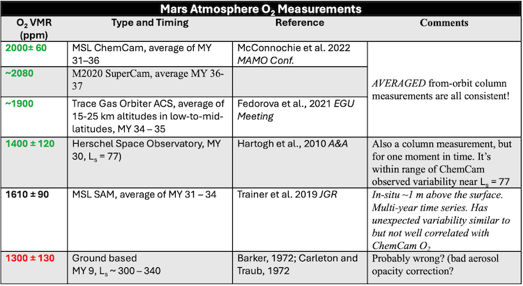
Table 1 shows an alternative approach to understanding the nature of the apparent O2 cycle, in this relying on long term averages of ChemCam and SuperCam measurements, compared to long term averages from SAM mass spectrometer in-situ atmospheric samples (Trainer et al. 2019), and to other available O2 measurements. What we see is that the measurements representative of column-averaged O2 are all consistent with each other and significantly higher than what SAM observes. This implies that there is a net sink for O2 near the surface at Gale crater and that that sink is relatively fast compared to vertical mixing time scales.

References: Barker, 1972, Nature, 238(5365), https://doi.org/10.1038/238447a0. Carleton and Traub, 1972, Science, 177(4053), https://doi.org/10.1126/science.177.4053.988. Fedorova et al., 2021 EGU Meeting. Hartogh et al., 2010, A & A, 521, https://doi.org/10.1051/0004‐6361/201015160. Klein, 1978, Icarus, 34(3), https://doi.org/10.1016/0019‐1035(78)90053‐2. ,Lefevre et al., 2004, JGR, 109, https://doi.org/10.1029/2004JE002268. Lo et al. 2024, PSJ 5, https://doi.org/10.3847/PSJ/ad251b.McConnochie et al., 2022, Mars Atmosphere Modeling and Observations Conference. McConnochie et al. 2024 10th Mars Conference.  Oyama & Berdahl, 1977, JGR, 82(28), https://doi.org/10.1029/JS082i028p04669.  Stcherbinine et al., 2026, EGU Meeting.  Trainer et al. 2019, JGR12, https://doi.org/10.1029/2019JE006175, Savijärvi et al. 2019, Icarus 326, https://doi.org/10.1016/j.icarus.2019.03.020. VanBommel et al. 2018, JGR, 123, https://doi.org/10.1002/2017JE005454. VanBommel et al. 2024, 10th Mars Conference. Yen et al, 2000, Science, 289(5486), https://doi.org/10.1126/science.289.5486.1909.

TABLE 1: Comparison of lower-atmosphere O2 mixing ratios from various sources                                           

FIGURE 1: Comparison of trace gas seasonal cycles at Gale Crater over 5 Mars years. Individual points are retrieval results for the indicated year and solar longitude, with 1-sigma error bars. The smooth lines for O2 are the result a LOESS regression and the shaded region around those smoothed lines represents the 1-sigma uncertainties of that LOESS regression. The “LMD model” for O2 and Ar is from Lefevre et al. (2004), but scaled so that the average model value matches the average observed value.The argon data in the top panel is from VanBommel et al. (2024) using methodology from VanBommel et al. (2018).

How to cite: McConnochie, T. and the Co-authors: Sky Spectroscopy with the Perseverance and Curiosity Mars Rovers: Latest results for Molecular Oxygen and Water Vapor, Europlanet Science Congress 2026, The Hague, The Netherlands, 7–11 Sep 2026, EPSC2026-312, https://doi.org/10.5194/epsc2026-312, 2026.

09:12–09:24
|
EPSC2026-199
|
ECP
|
On-site presentation
Meghna Dutta, Ladislav Rezac, Borys Dabrowski, and Paul Hartogh

We present new ground-based microwave observations of the diurnal variation of mesospheric ozone made over Göttingen, Germany, over four years from March 2022 to March 2026. These data are of high quality and characterise the diurnal behaviour of the ozone mixing ratio during the solstices and equinoctial conditions. The observed diurnal variation of ozone peaks at ~75 km. At 65 km, the observed diurnal variation is less than half, whereas at 50 km it is less than a quarter of the maximum variation. In this presentation, we compare measurements taken over different periods throughout the year and conduct a comprehensive data analysis. We compare it with satellite observations for further validation.

How to cite: Dutta, M., Rezac, L., Dabrowski, B., and Hartogh, P.: New High-Sensitivity Ground-Based Microwave Observations of Mesospheric Ozone. , Europlanet Science Congress 2026, The Hague, The Netherlands, 7–11 Sep 2026, EPSC2026-199, https://doi.org/10.5194/epsc2026-199, 2026.

09:24–09:36
|
EPSC2026-307
|
ECP
|
On-site presentation
Taishun Ao, Hiromu Nakagawa, Yannick Willame, Yuki Nakamura, Ian Thomas, Shohei Aoki, Frank Daerden, Lori Neary, Arianna Piccialli, Rebecca Jolitz, Ali Rahmati, and Naoki Terada

Ozone is an important trace gas for understanding the dynamics and photochemistry of planetary atmospheres and protecting life from harmful ultraviolet radiation on Earth. It is well known that ozone is efficiently destroyed by odd nitrogen (NOx) and odd hydrogen (HOx) generated by solar energetic particles (SEPs) on Earth [1]. It has never been proven that such phenomena can occur universally on the terrestrial planets. For instance, Mars lacks a global intrinsic magnetic field and has a thin CO2-dominated atmosphere, making it vulnerable to SEP impacts. Such SEP impacts are global and much closer to the surface than on Earth, as revealed by the global SEP aurora [2]. Nakamura et al. (2023) [3] predicted that such a space-atmosphere interaction induced by SEP would cause significant impacts on Mars’ atmospheric composition. Despite model predictions, observational understanding of such effects on Mars remains limited. This study aims to detect SEP-induced ozone depletion on Mars through observations.

In this study, we analyzed the absorption spectra of ozone around 200-300 nm obtained from the ultraviolet to visible (UVIS) channel of the NOMAD (Nadir and Occultation for MArs Discovery) instrument onboard the ExoMars Trace Gas Orbiter (TGO) [4]. We focused on the major SEP event in February 2024. During this event, three distinct peaks of SEP flux were observed by SEP measurements onboard MAVEN [5] over one month. Especially, the third peak shows a significant enhancement of the flux at 5 MeV ions, lasting for 4 days. Our Monte Carlo precipitation model, driven by SEP spectra measured by MAVEN/SEP, predicted that the SEP energy up to 5 MeV was sufficient to penetrate the Martian atmosphere down to ~50 km.

The ozone column density observed by NOMAD showed multiple decreases of approximately 10-20% at which timings coincided with the peak flux increase of the SEP event. However, regardless of the SEP, Martian ozone levels can naturally fluctuate due to factors such as clouds, atmospheric circulation, and dust. The remarkable point is that this global decline in ozone was observed simultaneously in both the northern and southern hemispheres. Such global ozone fluctuations are consistent with the predicted impact of the SEP event, rather than localized meteorological factors. This decrease is compared to our model prediction of ~10% decrease. Our result supports the model hypothesis that suggests water cluster ions (H⁺(H₂O)ₙ), generated by SEP, produce HOx compounds which destroy ozone in the CO2-dominated atmosphere. NOMAD observations demonstrate a global-scale ozone depletion coinciding with SEP penetration on Mars. This study presents remarkable observational results indicating that ozone depletion can occur due to SEPs even on planets with CO₂-dominated atmospheres, such as Mars. Understanding the impact of SEPs on Mars is crucial for elucidating the evolution of the Martian atmosphere from its early stages - when solar activity was more intense than it is today - to its current state.

References:

[1] Jackman et al. (2005) J. Geophys. Res., 110 A09S27.

[2] Schneider et al. (2018) Geophysical Research Letters, 45, 7391–7398.

[3] Nakamura et al. (2023) Earth, Plan. and Space, 75, 140.

[4] Vandaele et al. (2018) Space Sci. Rev., 214, 80.

[5] Larson et al. (2015 Space Sci. Rev., 195, 153.

How to cite: Ao, T., Nakagawa, H., Willame, Y., Nakamura, Y., Thomas, I., Aoki, S., Daerden, F., Neary, L., Piccialli, A., Jolitz, R., Rahmati, A., and Terada, N.: Global ozone depletion on Mars during major SEP events observed by TGO/NOMAD, Europlanet Science Congress 2026, The Hague, The Netherlands, 7–11 Sep 2026, EPSC2026-307, https://doi.org/10.5194/epsc2026-307, 2026.

09:36–09:48
|
EPSC2026-135
|
ECP
|
On-site presentation
Benjamin Benne, Paul Palmer, Franck Lefèvre, and Ehouarn Millour

Ozone is a key trace gas of the Martian atmosphere. It is produced through the photolysis of carbon dioxide followed by a three-body reaction between atomic and molecular oxygen. Its primary sinks are photodissociation, which recycles lighter odd oxygen (Ox) species, and gas-phase reactions with odd-hydrogen (HOx) species, which are produced by water vapour photolysis.

Many previous studies have shown that current Mars atmospheric general circulation models (GCMs) fail to reproduce the ozone columns observed by Mars Express and Mars Reconnaissance Orbiter studies (e.g. [1,2]), typically underestimating them by a factor of two [3].To help bridge the gap between models and observations, some studies examined the influence of various factors on the modelled ozone, including heterogeneous chemistry on water ice and dust aerosols, reaction rates, or radiative transfer [1,2]. These adjustments led to some local and temporally limited improvements, but often increased discrepancies elsewhere, suggesting that key processes may still be missing from Martian GCMs.

In this study, we adopt a different approach by investigating the propagation of chemical uncertainties using the 1-D sub-model of the Mars Planetary Climate Model (MPCM). We conducted a global sensitivity study using Monte Carlo simulations in which all reaction rates were randomly varied within their measured or estimated uncertainty ranges. Then, we identified correlations between the volume mixing ratios of key species (Ox and HOx) and reaction rates variations, which allowed us to determine which reactions most strongly influenced model outputs. We then adjusted the rates of these key reactions within the full GCM and found that doing so significantly improves simulated ozone VMRs relative to observations from the Atmospheric Chemistry Suite (ACS) onboard the ExoMars Trace Gas Orbiter (TGO). Based on our analysis, we recommend an assessment of these key reaction rates under relevant conditions, along with their implementation in GCMs, to better constrain the remaining discrepancies between models and observations.


References:

[1] Lefèvre, F., A. Trokhimovskiy, A. Fedorova, L. Baggio, G. Lacombe, A. Määttänen, J.‐L. Bertaux, et al., JGR: Planets 126, no. 4 (2021)

[2] Daerden, F., Crowley, J. N., Neary, L., Smith, M. D., Loeffler, M. J., Clancy, R. T., et al., JGR: Planets, 128, (2023)

[3] Olsen, K. S., A. A. Fedorova, A. Trokhimovskiy, F. Montmessin, F. Lefèvre, O. Korablev, L. Baggio, et al., JGR: Planets 127, no. 10 (2022)

How to cite: Benne, B., Palmer, P., Lefèvre, F., and Millour, E.: Reconciling Martian ozone with model photochemistry: new insights from an uncertainty propagation study, Europlanet Science Congress 2026, The Hague, The Netherlands, 7–11 Sep 2026, EPSC2026-135, https://doi.org/10.5194/epsc2026-135, 2026.

09:48–10:00
|
EPSC2026-519
|
ECP
|
On-site presentation
Paul Streeter, Kylash Rajendran, James Holmes, Stephen Lewis, Jonathon Mason, and Manish Patel

Introduction: Ozone is an important trace gas in the martian climate system. It is intimately linked to the odd-hydrogen (HOx) species (H, OH, HO2), low-abundance but highly reactive chemicals essential for maintaining the stability of Mars’ overwhelmingly CO2 atmosphere [1]. These HOx species are difficult to observe directly, but their presence can be inferred via their destruction of (and therefore anti-correlation with) ozone.

Ozone has a short photochemical lifetime on the dayside of a few hours. In the polar night, however, it is able to persist for significantly longer, allowing it to serve as a tracer for large-scale atmospheric dynamics, such as those associated with the polar vortices. Indeed, observed ozone has been shown to be closely correlated with modelled potential vorticity (PV, a diagnostic thermal-dynamical variable) in the polar winter [2].

Ozone observations can serve as valuable constraints for our understanding of both chemical and dynamical processes in the martian atmosphere. However, numerical models have long had issues in representing martian ozone, tending to underestimate total ozone abundance [e.g. 3]. Several tacks have been taken in trying to resolve this discrepancy, including incorporating heterogeneous chemical reactions (gas-solid; e.g. uptake of HOx species onto water ice clouds) and modifying existing reaction rates [e.g. 3,4]. While some improvement has resulted, model-observation disagreements remain.

In this work, we explore the impacts of data assimilation (see below) on the modelled ozone representation, and compare to retrieved ozone observations, in order to better characterise the model biases and the causal mechanisms behind them.

Approach: We employ a statistical technique called data assimilation. Data assimilation is a means for combining a numerical model of a system with discrete observations of that system; for example, a global climate model (GCM) of Mars with satellite observations of the martian atmosphere. By doing this, one can get the best of both worlds: the full spatio-temporal coverage and deterministic causal chain of the model, and the accuracy of actual observational data.

We use the Open University’s Mars GCM, also known as the Mars Planetary Climate Model – UK (PCM-UK) [5,6,7]. This shares model physics with the Mars PCM, but possesses a different dynamical core and data assimilation capability using the analysis correction scheme adapted from the UK Met Office [8].

We assimilate temperature profiles from the Mars Climate Sounder (MCS) and Atmospheric Chemistry Suite (ACS), together with water column and profile retrievals from ACS and the Nadir and Occultation for MArs Discovery (NOMAD) instrument. We do not assimilate ozone, but compare the model ozone to column retrievals from NOMAD-UVIS [9].

Results & Discussion: We present results comparing the baseline model simulation (“Control”), assimilated model simulation (“Assimilation”), and NOMAD-UVIS ozone retrievals (“Observations”) for the first half of Mars Year (MY) 36.

Preliminary results indicate that the Assimilation improves the fit with the Observations in some areas but worsens it in others, likely due to a wetter atmosphere in the Assimilation. At higher latitudes nearer the poles, both Control and Assimilation significantly underpredict total ozone column.

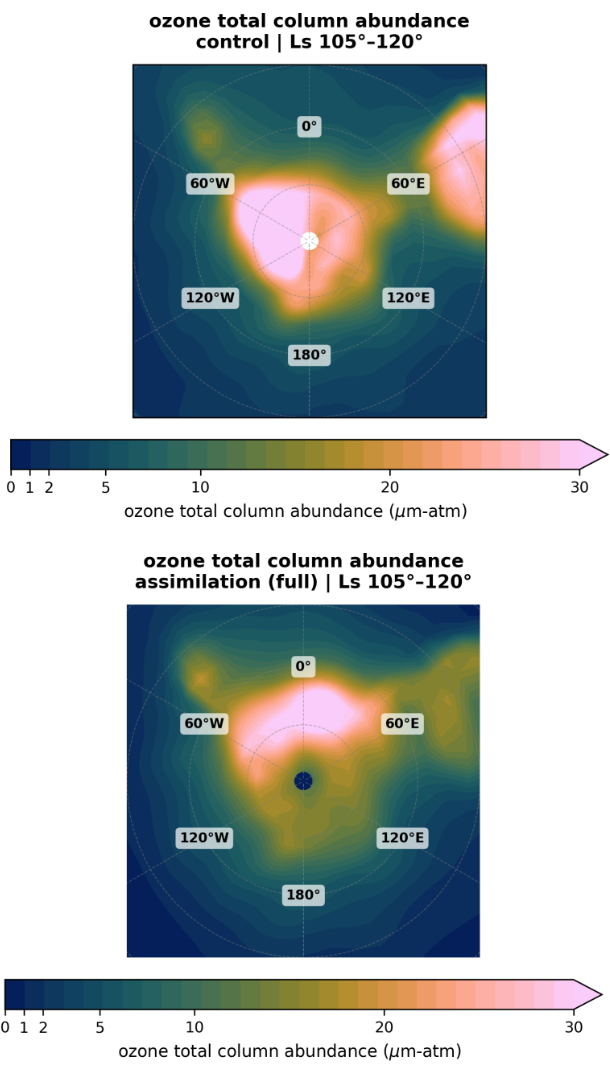
Over the southern winter pole, where Observations are unfortunately lacking, we find that the Assimilation and Control show radically different ozone distributions within the polar vortex. This appears to be due to the improved representation of the characteristic annular vortex structure in the Assimilation, where the PV maximum is located at least 10 degrees off-pole (see Fig. 1).

We discuss these and other results in the context of existing work. By comparing the ozone distribution in the two model simulations and the retrieved ozone, we can identify where model biases are due to missing chemistry/physics, and where they may be attributable to incorrect representation of other key atmospheric variables (such as temperatures and the water cycle).

Figure 1. Comparison of modelled ozone total abundance over the south pole between the Control (top) and Assimilation (bottom) for same period in MY 36.


References: [1] McElroy & Donahue (1972). Science. 177 (4053). [2] Holmes et al. (2017). Icarus. 282. [3] Lefèvre et al. (2021). JGR Planets. 126 (4). [4] Brown et al. (2022). JGR Planets. 127 (11). [5] Forget et al. (1999). JGR Planets. 104 (E10). [6] Lewis et al. (2007). Icarus. 192 (2). [7] Holmes et al. (2020). Planet. & Space Sci. [8] Lorenc et al. (1991). QJRMS. [9] Mason et al. (2024). JGR Planets.

How to cite: Streeter, P., Rajendran, K., Holmes, J., Lewis, S., Mason, J., and Patel, M.: Chemico-dynamical impacts of data assimilation on martian atmospheric ozone, Europlanet Science Congress 2026, The Hague, The Netherlands, 7–11 Sep 2026, EPSC2026-519, https://doi.org/10.5194/epsc2026-519, 2026.

Orals THU2: Thu, 10 Sep, 11:00–12:30 | Room Neptune (Spinoza Foyer)

Mars atmospheric composition (cont.) + Mars Aerosols
11:00–11:15
|
EPSC2026-869
|
ECP
|
On-site presentation
Vinayak Shastri, James Holmes, Manish Patel, and Stephen Lewis

Investigations into martian paleoclimatology have shown Mars in the past (~ 4 billion years ago) used to contain significant amounts of surface liquid water in contrast to present day conditions [1,2]. Given the importance of liquid water for life on Earth, understanding the evolution of the martian climate from a planet containing surface liquid water to a cold and dry planet today will improve our understanding of the conditions that influence terrestrial planetary habitable environments. Hydrogen escape is proposed as a major process in the depletion of water from Mars. This is where water molecules disassociated into hydrogen and oxygen after which hydrogen escapes the martian atmosphere through atmospheric escape processes such as Jeans escape and sputtering [3].

Previous investigations of martian hydrogen escape using a 1-D upper atmospheric model have shown that water loss rates on Mars are driven by the availability of water vapour near the boundary between the middle and the upper atmosphere (~ 80 km altitude), with water loss on Mars seasonally driven during perihelion and enhanced atmospheric dust activity such as regional and global dust storms (GDS) [4,5]. GDS events on Mars strongly influence interannual variations in the martian climate, occurring approximately every 5–10 Earth years, with the most recent GDS occurring in 2018 (hereafter referred to as martian Year 34 or MY34) [6]. The MY34 GDS also coincided with the start of the ExoMars Trace Gas Orbiter (TGO) observations, with TGO providing the greatest level of spatial coverage of water vapour profiles to date. These observations indicate enhanced transport of water vapour to the upper atmosphere [7,8,9].

Constraining the seasonal and interannual availability of water vapour in the upper atmosphere is therefore integral to determine the amount of water escaping from Mars. One such method of constraining is through data assimilation. This methodology combines the data of accurate but incomplete spatiotemporal observations of the martian atmosphere by orbiters with the complete spatiotemporal coverage albeit parameterised simulation of the martian atmosphere provided by models to reconstruct the martian atmosphere most in line with observations ensuring physical consistency. Recent work on data assimilation of TGO water vapour column and profiles into the Mars Planetary Climate Model UK-Spectral version (MPCM) has shown there is improved representation in the MPCM of water vapour profiles in line with orbiter observations around the upper atmosphere in contrast to free run simulations [10]. Therefore in this presentation, we explore the hydrogen escape flux using MPCM water cycle simulations based on data assimilation of TGO data.

The martian water cycle is simulated from LS = 160˚ in MY34 to the end of MY35 using the MPCM with data assimilation of ExoMars Trace Gas Orbiter water vapour column and profile measurements, alongside temperature profiles from Mars Reconnaissance Orbiter and dust optical depths from Mars Reconnaissance Orbiter and Mars Odyssey, to constrain the model’s atmospheric state and reproduce the martian water cycle in the most representative state. The outputs from the MPCM water cycle are coupled to the 1D upper atmosphere photochemical model from which the hydrogen escape is calculated from LS = 160˚ in MY34 to the end of MY35. The hydrogen flux during the MY34 GDS is compared to MY35 which is a martian year with nominal atmospheric dust levels.


Figure 1: MY34/MY35 Hydrogen escape flux ratio vs LS from MPCM simulations using data assimilation of ExoMars Trace Gas Orbiter water vapour profiles and columns along with Mars Reconnaissance Orbiter temperature profiles


We find that the hydrogen escape during the MY34 GDS is larger by a factor of 6 with respect to MY35 around LS = 195 – 215˚. There is also enhanced hydrogen escape by around 4 times in magnitude with respect to MY35 between LS = 330 – 345˚ in MY34 which correlates with the annual C – Type [6] regional dust storm activity which was considerably stronger in MY34 compared to MY35 (Figure 1). These results show there is enhanced water loss during increased atmospheric dust activity such as GDS and C-Type regional dust events, suggesting that interannual dust activity needs to be considered for long term martian water loss calculations. We present the reanalysis of the water cycle during the MY34 GDS and findings of the atmospheric processes influencing variations in the hydrogen escape flux. We will also present estimates for the interannual water loss from Mars based on MPCM water cycle simulations constrained by multi-orbiter assimilation.

Reference: [1] Ramirez, R.M. & Craddock, R.A. (2018) Nat. Geosci., 11, 230–237. [2] Pollack, J. et al. (1987), Icarus, 71(2), pp. 203–224. [3] Kasting, J.F. and Catling, D. (2003), Annu. Rev. Astron. Astrophys., 41(1), pp. 429–463. [4] Chaffin, M., Deighan, J., Schneider, N. et al. (2017), Nature Geosci 10, 174–178 [5] Holmes, J.A. et al. (2021) Earth Planet. Sci. Lett., 571, p. 117109. [6] Kass, D. et al. (2016), GRL, 43 (12), 6111-6118. [7] Vandaele, A. C. et al. (2018) Space Sci. Rev. 214(5). [8] Korablev, O. et al. (2018), Space Sci. Rev. 214(1), 7 (2018). [9] Aoki, S. et al. (2019), JGR (Planets) 124(12), 3482–3497. [10] Holmes, J.A. et al. (2022) JGR (Planets), 127(10).

How to cite: Shastri, V., Holmes, J., Patel, M., and Lewis, S.: Interannual variability in hydrogen escape from Mars and implications for water loss: Insights from ExoMars Trace Gas Orbiter data assimilation into a global climate model, Europlanet Science Congress 2026, The Hague, The Netherlands, 7–11 Sep 2026, EPSC2026-869, https://doi.org/10.5194/epsc2026-869, 2026.

11:15–11:27
|
EPSC2026-417
|
ECP
|
On-site presentation
Valentin Steichen, François Leblanc, Jean-Yves Chaufray, Mehdi Benna, Quentin Nenon, Ronan Modolo, and Shanon Curry

Argon is an inhert gas that can be used to measure different areas of thermal populations and non-thermal populations in the upper atmosphere of Mars. In this work, a statistical survey over 7 years' worth (2018-2024) of MAVEN/NGIMS measurements during Mars Year 35 – 37 (25,000+ standard survey orbits + 268 dedicated high-cadence argon orbits (1,100+) has been produced that provide reliable measurements from 150 km periapsis altitudes and up to 1200 km in the extended exosphere.

The thermal populations of argon in the thermosphere (150 – 300 km) have a pronounced diurnal variation with respect to solar-driven expansion. Temperatures derived from the scale height technique show a range of 150 K (dawn minimum around LST 3 - 6) to 300 K (afternoon maximum around LST 14 - 16) which results in a factor of 2 diurnal amplitude. Dayside temperatures in the thermosphere correlate strongly with EUVM Lyman-A irradiance as observed by EUVM indicating that the Ar thermosphere reacts to changing heliocentric as well as the Solar Cycles 24 – 25 transition with variations of 100 - 200 K, which indicates that dynamical effects (tides and gravity waves) also occurs.

At higher altitudes (above 400 km), Ar exhibits a coherent response to variations in UV flux  but experience reduced effective scale heights which is likely due to collisional damping. Increased EUV results in downward displacement of the O₂⁺ production layer into denser portions of the thermosphere, thereby increasing the column density above it and thermally stimulating the upward-moving suprathermal Ar resulting in more frequent collisions of the hot O and thus a partial thermalization.

On the night side,  high-altitude argon approaches NGIMS detection limits (~10 cm⁻³), while terminator passes reveal that the scale height temperature drastically inreases, which could be an indicator of a different suprathermal process than recombinative dissociation. Organized by SZA, altitude regime (thermal/transition/suprathermal), local time, season (Ls), latitude, and solar forcing, these results establish argon as a robust diagnostic of thermospheric dynamics, suprathermal production physics, terminator transport asymmetries, and baseline conditions for quantifying non-thermal neutral escape pathways at Mars.


Figure: Averaged distribution of the Ar corona at Mars

How to cite: Steichen, V., Leblanc, F., Chaufray, J.-Y., Benna, M., Nenon, Q., Modolo, R., and Curry, S.: A Statistical Survey of the Martian Argon Exosphere Using MAVEN  Data, Europlanet Science Congress 2026, The Hague, The Netherlands, 7–11 Sep 2026, EPSC2026-417, https://doi.org/10.5194/epsc2026-417, 2026.

11:27–11:39
|
EPSC2026-868
|
ECP
|
On-site presentation
Pablo Rodriguez-Ovalle, Miguel Angel Lopez-Valverde, Ashimananda Modak, Francisco Gonzalez-Galindo, Adrian Brines, Miguel Ángel Gamonal Gracía-Galán, Juan Alday, Alexander Trokhimoskiy, Denis A. Belyaev, Kevin S. Olsen, Franck Montmessin, Lucio Baggio, Anna A. Fedorova, Oleg I. Korablev, Frank Daerden, Ian R. Thomas, Ann Carine Vandaele, Manish R. Patel, and Giancarlo Bellucci

Carbon monoxide (CO) is one of the most important tracers of atmospheric circulation and photochemical activity in the Martian atmosphere. Because of its relatively long chemical lifetime, its spatial and vertical distribution is strongly linked to the large-scale transport processes that shape the Martian climate. At the same time, CO is directly connected to the CO₂ photochemical cycle, making it a valuable probe of the coupling between atmospheric dynamics and chemistry. Since its first detections through ground-based observations several decades ago [1,2], CO has been extensively investigated by orbiters and space missions dedicated to the exploration of Mars. These observations have revealed strong seasonal, latitudinal, and vertical variations, highlighting the complexity of the Martian atmosphere and the need for long-term, high-resolution measurements to better constrain atmospheric circulation and photochemical models.

The ExoMars Trace Gas Orbiter (TGO), launched in 2016, has significantly improved our capability to study trace species in the Martian atmosphere thanks to its high spectral resolution and global coverage. Among its scientific payload, two instruments are capable of observing CO: NOMAD and the Atmospheric Chemistry Suite (ACS) [3,4]. In particular, the ACS-MIR channel provides high-quality solar occultation measurements with exceptional sensitivity to the vertical structure of the atmosphere, allowing the retrieval of atmospheric profiles over a broad altitude range.

In this work, we analyze solar occultation spectra acquired by the ACS-MIR channel, focusing on the CO (2–0) overtone absorption band between 4150 and 4350 cm⁻¹. We describe in detail the preprocessing steps applied prior to the atmospheric retrievals, including corrections for spectral bending and wavelength shifts, as well as improvements in the characterization of the instrumental line shape [5]. Particular attention has been devoted to the refinement of the error budget in order to properly account for instrumental and spectroscopic uncertainties affecting the measurements. These improvements are essential to maximize the accuracy and stability of the retrievals, especially when combining information from lines with very different sensitivities throughout the atmosphere.

The spectra are analyzed using the KOPRA radiative transfer model coupled with the RCP inversion code [6] to retrieve vertical profiles of CO volume mixing ratio (VMR) and temperature. A detailed sensitivity analysis of the CO absorption lines at different atmospheric altitudes is also presented. Because the strongest CO lines become saturated below ~50 km, retrieving reliable information across the full atmospheric column requires a careful selection and combination of spectral lines probing different altitude regions. While saturated lines reduce sensitivity in the lower atmosphere, they remain crucial for constraining CO abundances in the upper atmosphere, particularly between ~80 and 120 km. To address this challenge, we developed a dedicated retrieval strategy that allows us to derive robust and continuous CO vertical profiles from the lower atmosphere up to the thermosphere.

In addition, we demonstrate for the first time the simultaneous retrieval of temperature and CO VMR from a dataset containing only CO absorption lines. This is possible because the full CO absorption band is observed: the overall shape of the band contains information about the atmospheric thermal structure, while the depth and relative intensity of the individual absorption lines constrain the CO abundance. The methodology developed for this simultaneous retrieval represents a significant step forward for the analysis of ACS-MIR observations, and a more detailed explanation of this approach will be presented in this work.

Using this method, we retrieve CO vertical profiles between ~7 and 120 km altitude and temperature profiles between ~7 and 100 km. We present temperature profiles for the first half of Mars Year (MY) 34 and compare them with other available datasets [8]. In addition, we show CO abundance maps covering MY 34 to MY 37, providing a multi-year overview of the seasonal and latitudinal variability of CO in the Martian atmosphere. The retrieved distributions are broadly consistent with previous studies [7,8], showing an approximately constant CO abundance below ~50 km and a marked increase at higher altitudes driven by photochemical production. Clear seasonal and latitudinal variations are also observed throughout MY 34–37, reflecting the influence of atmospheric transport and circulation processes. The implications of these results for our understanding of Martian atmospheric dynamics and photochemistry are discussed.


[1] Krasnopolsky, V. A. (2007). Icarus, 190(1), 93–102. https://doi.org/10.1016/j.icarus.2007.02.015

[2] Smith, M. D. (2004). Icarus, 167(1), 148–165. https://doi.org/10.1016/j.icarus.2003.09.010

[3] Vandaele, A. C. et al. (2018). Space Science Reviews, 214(5), 80. https://doi.org/10.1007/s11214-018-0517-2

[4] Korablev, O. et al. (2018). Space Science Reviews, 214(1), 7. https://doi.org/10.1007/s11214-017-0437-6

[5] López-Valverde, M. A. et al. (2023). J. Geophys. Res. Planets, 128(2), e2022JE007278. https://doi.org/10.1029/2022JE007278

[6] Stiller, G. P. (2000). FZKA Report, 6512, Forschungszentrum Karlsruhe.

[7] Modak, A. et al. (2023). J. Geophys. Res. Planets, 128(3), e2022JE007282. https://doi.org/10.1029/2022JE007282

[8] Fedorova, A. A. et al. (2022). J. Geophys. Res. Planets, 127(9), e2022JE007195. https://doi.org/10.1029/2022JE007195

How to cite: Rodriguez-Ovalle, P., Lopez-Valverde, M. A., Modak, A., Gonzalez-Galindo, F., Brines, A., Gamonal Gracía-Galán, M. Á., Alday, J., Trokhimoskiy, A., Belyaev, D. A., Olsen, K. S., Montmessin, F., Baggio, L., Fedorova, A. A., Korablev, O. I., Daerden, F., Thomas, I. R., Vandaele, A. C., Patel, M. R., and Bellucci, G.: Martian CO vertical distribution combining 4 Martian Years of TGO/ACS MIR solar occultation data, Europlanet Science Congress 2026, The Hague, The Netherlands, 7–11 Sep 2026, EPSC2026-868, https://doi.org/10.5194/epsc2026-868, 2026.

11:39–11:51
|
EPSC2026-722
|
On-site presentation
Adrian Brines, Shohei Aoki, Giuliano Liuzzi, Geronimo L. Villanueva, Sara Faggi, Shungo Koyama, Loïc Trompet, Ian R. Thomas, Miguel Angel Lopez-Valverde, Frank Daerden, Lori Neary, Sébastien Viscardy, Paul Palmer, Benjamin Benne, Manish R. Patel, Ann Carine Vandaele, Bojan Ristic, and Giancarlo Bellucci

Hydrogen chloride (HCl) is one of the most recent trace species discovered in the Martian atmosphere, renewing interest in the study of its climatology. Since its unambiguous detection by the Trace Gas Orbiter (TGO) in 2021 [1,2], several studies have focused on characterizing the spatial distribution and variability of this trace species and on understanding the processes controlling its presence in the atmosphere. Observations from the two TGO instruments capable of detecting HCl in solar occultation geometry, NOMAD and ACS, have consistently reported detections mainly during the second half of the Martian year, corresponding to the perihelion season and southern summer. These enhanced abundances are followed by a rapid decline toward the end of the year. During aphelion and northern summer, however, HCl detections from orbit remain rare and close to instrumental detection limits. This pattern has been observed repeatedly across multiple Martian years, with no noticeable interannual variability.

Several hypotheses have been proposed to explain the sources and sinks of HCl, its strong seasonal variability, and its preferential occurrence during perihelion. One possible source mechanism involves interactions between the surface and the atmosphere through the lifting of chlorine-bearing dust and subsequent reactions releasing chlorine species into the atmosphere. On the other hand, heterogeneous uptake by water ice particles has been proposed as a plausible sink for HCl [3, 4]. However, systematic observations of temporally and spatially collocated HCl and aerosol (dust and water ice) profiles are needed in order to provide further constraints on these hypotheses.

In this work, we present a climatology of HCl derived from four Martian years of NOMAD Solar Occultation observations. This instrument is an excellent asset for the detection and systematic monitoring of trace species in the Martian atmosphere. It provides high spectral resolution (λ/∆λ ∼ 17000) and high sensitivity thanks to the excellent signal-to-noise ratio achieved in the solar occultation geometry [5]. We investigated the seasonal and latitudinal variability of HCl vertical profiles throughout 5245 solar occultations, of which 291 profiles showed reliable HCl detections. We focused the analysis on the vertical structure and local time dependence of the retrieved profiles during the perihelion season, in addition to the study of correlations between HCl and other atmospheric species such as water vapor and aerosols. 

Our analysis confirms that HCl is primarily observed during southern summer, in agreement with previous studies analyzing orbital [1,2,6] and ground-based observations [7], while no robust detections are identified during the aphelion at tangent altitudes with optimum transmittance levels. Our results show that HCl is generally found at altitudes where water vapor abundances are enhanced, and both species exhibit a strong positive correlation, in agreement with previous studies [8]. We also observe a remarkably similar vertical structure of HCl at the morning and evening terminators. Finally, using collocated aerosol observations, we compare HCl distributions with dust and water ice abundances, finding a positive correlation with dust abundance but no clear correlation with water ice abundance.

References:

[1] Korablev, O., Olsen, K. S., Trokhimovskiy, A., Lef`evre, F., Montmessin, F., Fedorova, A. A., . . . others (2021). Transient HCl in the atmosphere of Mars. Science Advances, 7 (7),eabe4386

[2] Aoki, S., Daerden, F., Viscardy, S., Thomas, I. R., Erwin, J. T., Robert, S., . . . others (2021). Annual appearance of hydrogen chloride on Mars and a striking similarity with the water vapor vertical distribution observed by TGO/NOMAD. Geophysical Research Letters, 48 (11), e2021GL092506

[3] Taysum, B. M., Palmer, P. I., Olsen, K., Luginin, M., Ignatiev, N., Trokhimovskiy, A., . . . Korablev, O. (2024). Observed seasonal changes in Martian hydrogen chloride explained by heterogeneous chemistry. Astronomy & Astrophysics, 687 , A191.

[4] Luginin, M., Trokhimovskiy, A., Taysum, B., Fedorova, A. A., Korablev, O., Olsen, K. S.,. . . Lefevre, F. (2024). Evidence of rapid hydrogen chloride uptake on water ice in the atmosphere of Mars. Icarus, 411 , 115960.

[5] Vandaele, A. C., Lopez-Moreno, J.-J., Patel, M. R., Bellucci, G., Daerden, F., Ristic, B., . . . others (2018). NOMAD, an integrated suite of three spectrometers for the ExoMars trace gas mission: Technical description, science objectives and expected performance. Space Science Reviews, 214 (5), 1–47.

[6] Olsen, K. S., Fedorova, A. A., Kass, D. M., Kleinb¨ohl, A., Trokhimovskiy, A., Korablev, O. I., . . . others (2024). Relationships between HCl, H2O, aerosols, and temperature in the Martian atmosphere: 1. Climatological outlook. Journal of Geophysical Research: Planets, 129 (8), e2024JE008350

[7] Faggi, S., Aoki, S., Liuzzi, G., Villanueva, G., Sagawa, H., Mumma, M. J., . . . Viscardy, S. (2025). Following the HCl cycle over three Martian seasons in Mars year 36. Journal of Geophysical Research: Planets, 130 (11), e2025JE009105.

[8] Olsen, K., Fedorova, A., Kass, D., Kleinb¨ohl, A., Trokhimovskiy, A., Korablev, O., . . . others (2024). Relationships between HCl, H2O, aerosols, and temperature in the Martian atmosphere: 2. Quantitative correlations. Journal of Geophysical Research: Planets, 129 (8), e2024JE008351.

How to cite: Brines, A., Aoki, S., Liuzzi, G., Villanueva, G. L., Faggi, S., Koyama, S., Trompet, L., Thomas, I. R., Lopez-Valverde, M. A., Daerden, F., Neary, L., Viscardy, S., Palmer, P., Benne, B., Patel, M. R., Vandaele, A. C., Ristic, B., and Bellucci, G.: Vertical Structure and Variability of HCl in the Martian Atmosphere Observed by TGO-NOMAD., Europlanet Science Congress 2026, The Hague, The Netherlands, 7–11 Sep 2026, EPSC2026-722, https://doi.org/10.5194/epsc2026-722, 2026.

11:51–12:03
|
EPSC2026-879
|
ECP
|
On-site presentation
Bethan Gregory, Kevin Olsen, Ehouarn Millour, Megan Brown, Kylash Rajendran, Paul Streeter, Manish Patel, and Franck Lefèvre

Despite constituting a tiny fraction of the Mars atmosphere, trace gases can play an important role in controlling atmospheric chemical cycling. However, some discrepancies between observed distributions of trace gases and modelled values indicate that there are ongoing processes in Mars’ atmosphere that are not fully understood.

Hydrogen chloride (HCl) was the first new gas detected by the ExoMars Trace Gas Orbiter (TGO)[1,2], with observations from the Atmospheric Chemistry Suite (ACS) and Nadir and Occultation for Mars Discovery (NOMAD) instruments showing a strong seasonal variation over the last several Mars years. With a few exceptions, detections almost exclusively occur during the second half of the year (at solar longitudes between 180° and 360°). This is during southern hemisphere spring and summer, when temperatures, atmospheric dust content, and water vapour concentrations are higher, and ozone concentrations are low. Previous modelling has shown that heterogeneous chemical reactions involving dust or ice aerosols play a key role in controlling this seasonal pattern[3,4,5,6].

Here we use the Mars Planetary Climate Model[7,8], a 3-D global circulation model with photochemistry, to investigate some potential sources and sinks of HCl in the Martian atmosphere, which could account for the seasonal variation in measurements and the observed correlations and anticorrelations with other atmospheric factors. Firstly, we examine the indirect effect of heterogeneous chemistry of OH and HO2 interacting with ice. We compare the effect of two different heterogeneous chemical schemes[9,10] on HCl distributions via their effect on other oxidative species such as O and O3. Secondly, we investigate the isolated effects of two further heterogeneous pathways involving water ice—one HCl source and one sink. Specifically, we model the uptake of HCl onto water ice, which has been studied before, and its subsequent release back to the atmosphere during ice sublimation, which has not been included in previous models.

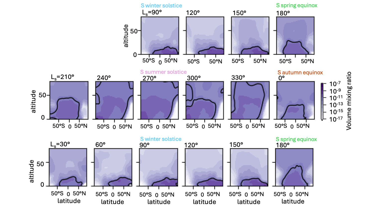
Our preliminary results (e.g., Figure 1) show that the latter cycling could account for some of the seasonality of the HCl observations. HCl concentrations remain close to the ground during the first half of the year, and then increase at higher altitudes during the second half of the year, where they could be detected by TGO's instruments. Even without the addition of other HCl sources and sinks in the model, we expect this pattern to be repeated over multiple Mars years, reproducing at least part of the annual appearance and disappearance of HCl through the recycling of chlorine.

Continuing to reconcile models and observations of the cycling of HCl and other trace gases is important for achieving a more complete understanding of atmospheric processes operating on Mars today, as well as those that have played a key role over Mars’ history.

Figure 1: Preliminary model results showing seasonal distributions of HCl over more than one Mars year. Each panel shows zonally-averaged HCl volume mixing ratios with altitude and latitude, and there are 30° of solar longitude between each panel. The black contour indicates a mixing ratio of 0.5 ppbv, which is the detection limit for TGO ACS.

[1] Korablev O. I. et al. (2021). Sci. Adv., 7, eabe4386. [2] Olsen K. S. et al. (2021). Astron. Astrophys., 647, A161. [3] Benne, B., et al. (2025). Astron. Astrophys., 699, A362. [4] Rajendran, K. et al. (2025). JGR: Planets 130(3), p.e2024JE008537. [5] Streeter, P. M. et al. (2025). GRL 52(6), p.e2024GL111059. [6] Taysum, B. M. et al. (2024). Astron. Astrophys., 687, A191. [7] Forget, F., et al. (1999). JGR: Planets 104, E10. [8] Lefèvre, F., et al. (2004). JGR: Planets 109, E7. [9] Brown M. A. J. et al. (2022). JGR: Planets, 127, p.e2022JE007346. [10] Lefèvre, F., et al. (2021) JGR: Planets126, p.e2021JE006838.

How to cite: Gregory, B., Olsen, K., Millour, E., Brown, M., Rajendran, K., Streeter, P., Patel, M., and Lefèvre, F.: Modelling interactions with ice to understand the seasonal variation of HCl, Europlanet Science Congress 2026, The Hague, The Netherlands, 7–11 Sep 2026, EPSC2026-879, https://doi.org/10.5194/epsc2026-879, 2026.

12:03–12:15
|
EPSC2026-106
|
ECP
|
On-site presentation
Francisco Brasil, Pedro Machado, Gabriella Gilli, Henrique Eira, Alejandro Cardesin-Moinelo, Valentin T. Bickel, Daniela Tirsch, John Carter, Nicolas Thomas, José E. Silva, Daniela Espadinha, Patrick Martin, and Colin Wilson

Atmospheric gravity waves (AGWs) are dynamically relevant in the Martian atmosphere [1], but orbital observations still provide an incomplete view of their morphology, altitude, and propagation conditions. Individual orbital images of clouds can identify wave packets and measure horizontal wavelengths, yet altitude, background wind, intrinsic phase speed, and vertical wavelength are only available when the observing geometry allows additional retrievals. This limits how far morphology alone can be interpreted dynamically. We compare three orbital datasets, that include clouds, each with different spatial resolution, coverage, and observing modes/geometry. They are not treated as a single climatology, because they cover different observing periods and have different sampling biases. Instead, we use them to test what part of the Martian AGW population each instrument can detect and characterize.

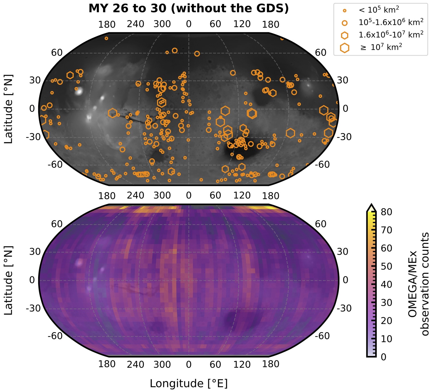
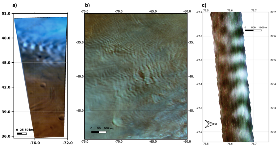
OMEGA/Mars Express nadir observations [2] during MY26–29 provide the widest occurrence baseline (Figure 1- a), although with a limited total number of observations. In this dataset, 263 wave packets were detected and 125 were characterized, with horizontal wavelengths from 6 to 83 km and a mean of 21 km [3]. Detections are concentrated in the northern hemisphere, especially at mid-to-high latitudes, with seasonal peaks during northern spring and autumn and southern winter. Their spatial distribution is consistent with topographic forcing near Tharsis–Alba and with convective activity over the northern plains. HRSC/Mars Express stereo-temporal imaging [4] during MY34–37 adds altitude and motion information (Figure 1- b). Wave packets identified in the HRSC Cloud Atlas [5] were characterized using blue-green inter-channel parallax to retrieve cloud-top altitude and approximately 30-minute repeat-track pairs to estimate horizontal motion. Retrieved altitudes are mostly 15–40 km, with uncertainties of about 3–10 km and a smaller number of cases extending to 60–100 km. For 11 packets with altitude, wind, and wave-geometry constraints, the analysis gives intrinsic phase speeds of 0.4–6.2 m/s and implied vertical wavelengths of 0.2–3.4 km under linear gravity wave assumptions [6]. Comparison with MCD static stability and background winds [7,8] indicates that some packets lie close to critical or turning levels, which may affect whether they remain visible at cloud level.

CaSSIS/ExoMars TGO imaging at 4 m/pixel [9] provides a substantially larger image dataset than HRSC, by roughly an order of magnitude, and samples smaller structures (Figure 1- c, Eira et al, in prep[10]). This part of the analysis remains preliminary, but it reaches sub-kilometer and few-kilometer horizontal wavelengths, below the OMEGA and HRSC detection ranges. A first comparison of spatiotemporal distribution, morphology, spatial scale, and observing geometry is used to assess instrument-dependent detection biases [10]. Whether the CaSSIS detections form the short-wavelength end of the OMEGA–HRSC population, or represent a separate subset controlled by different sources or visibility conditions, remains open.

Taken together, the datasets connect measurements that are usually obtained separately: morphology from cloud images, altitude from stereo geometry, and propagation constraints from repeat imaging and background winds. The comparison separates morphology-only detections from cases where altitude and wind information allow dynamical interpretation. These are the quantities needed to test how gravity wave drag is represented in Mars general circulation models.

Figure 1. Examples of Martian atmospheric gravity wave packets observed with (a) OMEGA/Mars Express, (b) HRSC/Mars Express, and (c) CaSSIS/ExoMars TGO, illustrating the different spatial scales and observing geometries used in the multi-instrument comparison.


Acknowledgments: This work was supported by the Portuguese Fundação para a Ciência e a Tecnologia through the research grant UID/04434/2025, and through the grants of reference 2021.05455.BD, and 2020.06389.BD. GG acknowledges financial support from Junta de Andalucía through the program EMERGIA 2021 (EMC21_00249) and from the Severo Ochoa grant CEX2021-001131-S funded by MCIN/AEI/10.13039/501100011033. IAA is also supported by grant ID2022-137579NB-I00 funded by MCIN/AEI/10.13039/501100011033 and by "ERDF A way of making Europe", funded by the ESA Faculty Research Contract and Science Exchange Programme, which is in the frame of the MWWM Mars Wind and Wave Mapping project of reference ESA RFP/3-17570/22/ES/CM. We also thank Lucie Riu, Aurélien Stcherbinine, and the Mars Express and ExoMars TGO Teams for their support and encouragement in this work.

References: [1] Fritts & Alexander, 2003; [2] Bibring et al., 2007; [3] Brasil et al., 2025; [4] Jaumann et al., 2007; [5] Tirsch et al., 2024; [6] Brasil et al. (under review); [7] Forget et al., 1999; [8] Millour et al., 2018; [9] Thomas et al., 2017; [10] Eira et al. (in prep.). 

How to cite: Brasil, F., Machado, P., Gilli, G., Eira, H., Cardesin-Moinelo, A., T. Bickel, V., Tirsch, D., Carter, J., Thomas, N., E. Silva, J., Espadinha, D., Martin, P., and Wilson, C.: Martian atmospheric gravity waves across scales: morphology, altitudes, and dynamics from MEx/OMEGA, HRSC, and ExoMars TGO/CaSSIS, Europlanet Science Congress 2026, The Hague, The Netherlands, 7–11 Sep 2026, EPSC2026-106, https://doi.org/10.5194/epsc2026-106, 2026.

12:15–12:27
|
EPSC2026-871
|
ECP
|
On-site presentation
Aurélien Stcherbinine, Tanguy Bertrand, Michael Wolff, Jérémie Lasue, Timothy McConnochie, Franck Montmessin, Thierry Fouchet, Elise Knutsen, Gaetan Lacombe, Agnes Cousin, Olivier Gasnault, Sylvestre Maurice, and Roger Wiens

Introduction

The SuperCam instrument onboard the Mars2020 Perseverance rover is a suite of remote sensing instruments that is operating on the Martian surface since February 2021 [1, 2, 3]. It notably includes a Visible-InfraRed (VISIR) spectrometer covering the 385–465 nm, 536–853 nm, and 1.3–2.6 µm spectral ranges [4], which regularly performs observations of the Martian atmosphere using the passive sky geometry to retrieve information on the composition of the atmosphere [5, 6]. At these wavelengths, scattering by aerosols is strongly sensitive to the particle size. The ability of the passive sky technique to retrieve the atmospheric dust content has been demonstrated in the VIS spectral range with MSL/ChemCam [7], and SuperCam is now able to probe for the first time the Martian atmosphere from the ground for both the VIS and near-IR domains, which provides further information on the aerosol properties.

Dust and water ice aerosols play an important role in the current Martian climate: they affect the thermal structure of the atmosphere as they absorb and scatter the incoming sunlight, and play an important role in the global water cycle of the planet [8]. Thus, monitoring the properties of these aerosols is of importance to better understand and model the current Martian climate. On Perseverance, the optical depth of the aerosols above the rover is monitored on a seasonal and local time basis by the MEDA and MastCam-Z (ZCAM) instruments [9-11].

Data & Methods

Regular Passive Sky

By measuring the spectra of the sky luminosity at two different elevation angles, and by comparing the measurement with the results of a multiple scattering radiative transfer model, we are able to retrieve the aerosol properties for both the dust and water ice over more than two Martian years. Here we use the DIScrete Ordinate Radiative Transfer (DISORT) code in version 4 [12] through the pyRT_DISORT Python module [13] to retrieve the respective optical depth of dust and water ice from the VISIR passive sky measurements of SuperCam performed since the beginning of the mission in 2021, and constrain their particle size. We assume asymmetric hexahydra dust particles and droxtals shapes for the water ice crystals, and we use vertical atmospheric profile from the Mars Climate Database version 6.1 [14, 15].

These retrievals complement the ones performed by the rover’s other instruments, notably ZCAM. While it is highly challenging with their measurements to distinguish between dust and water ice contributions in the total optical depth, their results can be directly compared with those from SuperCam, as the wavelength ranges of the two instruments overlap in the visible.

Thus, we assume the total column-integrated optical depth of the aerosols to be the same as the one derived by ZCAM at λ=880 nm, then we perform the retrievals on the relative amount of dust and ice, and on their particle size. In order to address the issue of local minima of the χ2 when performing the retrievals, we run the solver on a range of values for the particle sizes, then compare the χ2 values of all the runs to select the best fit.

Aerosols-specific Passive Sky

In addition to the regular passive sky performed at two altitudes, an other observation sequence has been implemented and run a few times on Mars with a series of measurements at the same altitude but for different azimuths. This allows to scan the lobe of the phase function of the scattering of the aerosols.

Comparison with MastCam-Z

On sols 1523 and 1563, two coordinated observations between SuperCam and MastCam-Z have been performed to compared the radiances measured by both instruments in the same regions of the sky, using the ZCAM filters whose wavelengths overlap with the SuperCam spectra range. These observations have been designed to investigate a potential straylight effect in the SuperCam passive sky data, but also provide an opportunity to compare and cross-calibrate the atmospheric retrievals between the two instruments.

Conclusion & Perspectives

For more than two Martian years now, the SuperCam instrument has been performing passive sky observations of the Martian atmosphere in the VISIR. Despite being challenging to perform, the aerosols retrievals from SuperCam provide information on the nature and particle size of the Martian aerosols in the lower layers of the atmosphere, and complement the measurements from the other instruments of the rover.

References

[1] Maurice et al. (2021) Nature, 605, 653-658. [2] Wiens et al. (2020) SSR, 217, 4. [3] Cousin et al. (2026) This conference. [4] Fouchet et al. (2022) Icarus, 373, 114773. [5] Bertrand et al. (2022) 7th MAMO, #1549. [6] McConnochie et al. (2026) This conference. [7] McConnochie et al. (2018) Icarus, 307, 294-326. [8] Haberle et al. (2017) The Atmosphere and Climate of Mars. [9] Toledo et al. (2024) Comm Earth & Env, 5, 717. [10] Smith et al. (2025) Icarus, 425, 116313. [11] Moya-Blanco et al. (2026), EGU 2026, EGU26-8137. [12] Stamnes et al. (2017), Astrophysics Source Code Library. 1708.006. [13] Connour & Wolff (2024) GitHub Repository, v1.2.0. [14] Forget et al. (1999) JGR, 104, 24155-24176. [15] Millour et al. (2024) EPSC 2024, EPSC2024-516.

How to cite: Stcherbinine, A., Bertrand, T., Wolff, M., Lasue, J., McConnochie, T., Montmessin, F., Fouchet, T., Knutsen, E., Lacombe, G., Cousin, A., Gasnault, O., Maurice, S., and Wiens, R.: Retrieving the Properties of Martian Aerosols at Jezero Crater over Two Martian Years using SuperCam Passive Sky Observations, Europlanet Science Congress 2026, The Hague, The Netherlands, 7–11 Sep 2026, EPSC2026-871, https://doi.org/10.5194/epsc2026-871, 2026.

12:27–12:30

Orals THU3: Thu, 10 Sep, 14:00–15:30 | Room Neptune (Spinoza Foyer)

Mars Aerosols (cont.)
14:00–14:15
|
EPSC2026-536
|
ECP
|
solicited
|
On-site presentation
Ethan Larsen, Agustín Sánchez-Lavega, Teresa del Río-Gaztelurrutia, and Jorge Hernández-Bernal

Following our report of new cases of extremely long and narrow mid-latitude clouds at Thaumasia Highlands (267°E, 39°S), Alba Patera (250°E, 40°N) and Lyot crater (29.3°E, 50.4°N) (Larsen et al., 2026), we analyze the Planetary Climate Model (PCM) (Forget et al., 1999)  predictions in order to understand the conditions under which they form. For this study, we take into account the predicted water vapor concentrations and temperatures, as well as the wind regime (velocity and direction).

We see that elongated clouds form when wind speeds close to the surface are higher (20 m/s at the origin point) compared to those during spring and summer. The same happens at higher heights, where horizontal wind speeds are far greater during fall and winter. In regards to wind direction and cloud orientation, cloud orientations at Thaumasia and Lyot agree with the predicted wind direction at 10 – 22 km and 5 – 16 km respectively, while at Alba Patera, there is a discrepancy. At the volcano, winds matching the initial cloud orientation are located higher up (∼40-50 km).

Orographic clouds, both on Earth and Mars, often reveal the presence of mountain waves. Since there are many types of mountain waves, and each produces a different type of cloud, identifying a particular type of wave can help understand and deduce certain atmospheric parameters, such as, wind speed and stability. Therefore, in order to see if the formation of these clouds is consistent with the model’s atmosphere, we have used a simple, single layered, two-dimensional model (Houze 2014) to understand the flow over arbitrary “bell shaped ridges” roughly the same shape of the aforementioned obstacles. In order to examine the fundamental properties of the mountain waves, we consider a steady-state, two-dimensional airflow, so that linear theory can be used. Linearazing and combining the equations for an inviscid Boussinesq fluid one can obtain a single equation for the vertical wind speed,  wzz + wxx + l2w = 0  (Durran 1986), where l is the Scorer parameter (Scorer 1949).  With the basic state wind profile and static stability, considered to be those upstream, and the aid of the continuity equation (ux +wz = 0),  we obtain the streamlines in the steady airflow over the ridges.

Figure 1. (a) Elongated cloud that forms at Warrego Rise (Thaumasia Highlands) on January 5th 2025 (MY38, Ls=26°). The dot marks the head or beginning of the cloud, while the arrows point at the tail. (b) Streamlines in the steady airflow over an isolated bell-shape similar in size to Warrego Rise for a Scorer value of l=0.00018 m-1 . The red solid line is the zonal topographic profile of Warrego Rise (x=0 at 267.3°E, 40.4°S).

The streamlines that describe the steady airflow are very dependant on the Scorer parameter and the size of the obstacle. Therefore, vertical displacement is seen to depend very much on the details of the airstream, such as, atmospheric stability and wind speed. Obtaining the vertical stability and wind speeds from the PCM we are able to calculate the vertical displacements and, with the vertical temperature and water abundance profiles, see if clouds similar to the ones observed are obtained.


References

Durran, D.R. (1986) Mountain Waves. In: Ray, P.S. (eds) Mesoscale Meteorology and Forecasting. American Meteorological Society, Boston, MA. https://doi.org/10.1007/978-1-935704-20-1_20

Forget, F. et al. (1999) Improved general circulation models of the Martian atmosphere from the surface to above 80 km. J. Geophys. Res. Planets 104, 24155–24175

Houze, R. A., Jr. (2014) Clouds and Precipitation Associated with Hills and Mountains. In International Geophysics (pp. 369–402). Elsevier. https://doi.org/10.1016/B978-0-12-374266-7.00012-3

Larsen, E. et al. (2026) Orographic elongated clouds in mid-temperate and subpolar latitudes of Mars. I-Observations. Icarus, 445, 116864. https://doi.org/10.1016/j.icarus.2025.116864

Scorer, R. S. (1949) Theory of waves in the lee of mountains. Quarterly Journal of the Royal Meteorological Society, 75(323), 41–56. https://doi.org/10.1002/qj.49707532308

How to cite: Larsen, E., Sánchez-Lavega, A., del Río-Gaztelurrutia, T., and Hernández-Bernal, J.: Interpretation of the extremely long and narrow mid-latitude orographic clouds on Mars, Europlanet Science Congress 2026, The Hague, The Netherlands, 7–11 Sep 2026, EPSC2026-536, https://doi.org/10.5194/epsc2026-536, 2026.

14:15–14:27
|
EPSC2026-119
|
On-site presentation
Lucas Lange, Francois Forget, Jean Baptiste Clément, Joseph Naar, Eran Vos, and Elad David

The present-day Martian climate is governed by three major cycles: CO2, water, and dust. Every winter, approximately 30% of the atmospheric condenses to form the seasonal CO2 caps [1]. In spring, these caps disappear, triggering surface activity such as CO2 geysers and contributing to the formation of gullies [2,3]. In late spring, the perennial North pole ice cap begins to sublimate, injecting water vapor into the dry atmosphere, forming thin clouds at mid and low latitudes, and millimetric night frost forms at the surface that vanishes by early morning [4].

This climate may have been more pronounced in the past due to the planet's orbital variations, and in particular its obliquity, which varied by as ±15° in the recent past [5]. Climate models show that during high-obliquity periods the polar night would be more extensive, intensifying the CO2 cycle, and that the amount of water vapor injected from the North Polar cap would be greater due to higher summer insolation [6]. Recent studies [e.g, 7] have notably shown that water ice clouds forming following this summer injection play a key role in Martian paleoclimates: by absorbing solar radiation, they warm the atmosphere, which can then hold more water vapor, producing larger clouds and creating feedback mechanisms that make the Martian atmosphere far more humid than it is today. While most models suggest that the CO2 cycle was more pronounced than today, a recent study by [8] shows that higher atmospheric humidity could promote the formation of pore-filling ground ice at mid- to low latitudes, thereby limiting the amplification of the CO2 cycle.

A second effect of these clouds is the warming of the surface. These clouds emit infrared radiation toward the surface, which can be significant during periods of low solar insolation such as winter or nighttime. On present-day Mars, this warming can reach 10 to 15 K at night in equatorial regions [9] Given how significant this effect already is today, the question of its impact on Martian paleoclimates naturally arises given the greater cloud abundance expected under past conditions. Yet it has never been studied to date.

In this presentation, we will discuss the surface warming induced by the downwelling infrared flux emitted by these clouds. We will show in particular that for obliquities above 35°, this warming is large enough that surface temperatures can no longer reach the CO2 condensation point over most of the Martian surface. As a result, the CO2 cycle, a defining feature of the present Martian climate, nearly disappears entirely under past high-obliquity conditions. Surface activity driven by CO2 condensation and sublimation is therefore not representative of recent surface history. In particular, we will show that if CO2 is indeed the agent responsible for forming the enigmatic Martian gullies, then these features could only have formed during low-obliquity periods below 30°, which is consistent with their young age [10]. Finally, while previous studies suggest that water ice could form within the pore spaces of dusty equatorial regions during high-obliquity periods [e.g., 8,11], we will show that this is unlikely due to surface warming. The presence of water-ice deposits within the pores of the upper equatorial regolith is therefore unlikely, although remnants of past massive ice sheets may still persist today [12,13].

References :

[1] Titus et al., 2017: The CO2 Cycle, in The Atmosphere and Climate of Mars, Cambridge University Press.

[2] Diniega et al., 2021: Modern Mars’ geomorphological activity, driven by wind, frost, and gravity, in Geomorphology, 380, 107627. DOI : 10.1016/j.geomorph.2021.107627 .

[3] Dundas et al., 2021: Active Mars: A Dynamic World, in Journal of Geophysical Research: Planets, 126(8). DOI: 10.1029/2021je006876.

[4] Montmessin et al., 2017: The water Cycle, in The Atmosphere and Climate of Mars, Cambridge University Press.

[5] Laskar et al., 2004: Long term evolution and chaotic diffusion of the insolation quantities of Mars, in Icarus, 170(2), 343–364. DOI: 10.1016/j.icarus.2004.04.005.

[6] Forget et al., 2017: Recent Climate Variations, in The Atmosphere and Climate of Mars, Cambridge University Press.

[7] Madeleine et al., 2014: Recent Ice Ages on Mars: The role of radiatively active clouds and cloud microphysics, in Geophysical Research Letters, 41(14), 4873–4879. DOI: 10.1002/2014gl059861.

[8] David et al., 2024: The Effect of Ground Ice Redistribution on the Martian Paleo‐CO2 Cycle., in Journal of Geophysical Research: Planets, 130(1). DOI: 10.1029/2024je008398

[9] Wilson et al., 2007: Diurnal variation and radiative influence of Martian water ice clouds, in Geophysical Research Letters, 34(2). DOI: 10.1029/2006gl027976

[10] de Haas et al, 2017: Time will tell: temporal evolution of Martian gullies and palaeoclimatic implications, in Geological Society, London, Special Publications, 467(1), 165–186. DOI: 10.1144/sp467.1

[11] Aharonson et al., 2026: Milankovitch forcing of equilibrium ground-ice on Mars, Icarus, 444, 116772. DOI: 10.1016/j.icarus.2025.116772

[12] Forget et al,  2006: Formation of Glaciers on Mars by Atmospheric Precipitation at High Obliquity, Science, 311(5759), 368–371. DOI: 10.1126/science.1120335

[13] Vos et al., 2026, The Martian mid-latitude subsurface ice is the remnant of a past ice sheet, Communications Earth & Environment. DOI: 10.1038/s43247-026-03418-x

How to cite: Lange, L., Forget, F., Clément, J. B., Naar, J., Vos, E., and David, E.: Surface Warming Induced by the Radiative Effect of Water Ice Clouds in the Late Amazonian: Implications for (Sub)-Surface Activity, Europlanet Science Congress 2026, The Hague, The Netherlands, 7–11 Sep 2026, EPSC2026-119, https://doi.org/10.5194/epsc2026-119, 2026.

14:27–14:39
|
EPSC2026-699
|
ECP
|
On-site presentation
Miguel Ángel Gamonal García-Galán, Miguel Ángel López Valverde, Adrián Brines, Aurelièn Stolzenbach, Ashimananda Modak, Bernd Funke, Pablo Rodríguez Ovalle, Juan Alday, Ian Thomas, Manish Patel, Giancarlo Bellucci, Frank Daerden, Bojan Ristic, and Zachary Flimon

Introduction

The Martian atmospheric aerosols are mainly composed of mineral dust and/or water ice. Water ice clouds affect both the radiative balance [1] and the water cycle [2], while mineral dust is globally the most abundant component, modifying the thermal structure and atmospheric dynamics [3,4]. It can affect observations from both orbiting satellites and rovers on ground, especially at the dusty season around perihelion, where many storms are initiated at different temporal and spatial scales [5].

Both aerosol types are related, as dust can serve as a base for water ice cloud formation [5]. Therefore, a comprehensive understanding of the Martian atmosphere requires a simultaneous climatology of both components, such as the one presented in this work.

Dataset and methodology

NOMAD is a three spectrometers suite on board the Trace Gas Orbiter (TGO). It has been routinely observing the Martian atmosphere since April 2018 [6], providing detailed atmospheric transmission vertical profiles. Data acquired from its solar occultation (SO) channel are used to retrieve aerosol properties and their vertical distributions in the infrared at high vertical resolution. This is achieved by combining multiple diffraction orders (i.e., wavelength intervals), selected to maximize coverage of the SO spectral range while consistently including an order near 3 μm. This spectral region is key to distinguish between dust and water ice aerosols [6].

Our retrieval strategy builds on [7] and is thoroughly described there. The inferred aerosol characteristics using this methodology are size (effective radius and variance) and composition (proportions of mineral dust and water ice). These magnitudes are used to derive other aerosol magnitudes such as number density, mass loading and mass mixing ratio.

We processed ~3000 SO observations from Ls = 194° (MY34) to the end of MY37, significantly extending the dataset in [7], focused only on the first year of NOMAD observations. We have also developed a scheme to identify cases with mixed aerosol components (dust and ice) from those where there is a single dominant component, and the secondary one is only adding noise to the results.


Results

In contrast to [7], due to our extended dataset we can study latitudinal and interannual comparisons between the different Martian Years, being able to detect the global patterns that govern the distribution of dust and water ice clouds.

We report an average maximum altitude of aerosol detection around 60 km near perihelion (Ls ~ 270°) and 40 km near aphelion (Ls ~ 90°). Variations within these values are sometimes significant, and linked to the latitude of the observations. Our results reveal features such as water ice clouds and signatures of both regional and global dust storms. All four Martian Years show systematic differences of their aerosol properties between aphelion and perihelion, which is consistent with the previous work by [7].

Lastly, a comparison of our results with similar datasets from NOMAD-UVIS [8] and ACS [9] has been performed. This comparison focuses on comparing the extinctions and effective radius retrieved, as well as their seasonal and latitudinal distribution. We have found that NOMAD-UVIS retrieves in average smaller particle sizes than SO, which is more sensitive lo larger sizes. Therefore, both wavelength ranges, ultraviolet and infrared, are complementary to produce a complete climatology of Martian aerosols. This combined information is important for improving climate models, which rely on a priori assumptions about aerosol microphysics, composition, and optical properties.


References:


  • Wilson, R.J, et. al., 2008.
  • Montmessin, F. et. al, 2004.
  • Michael Battalio and Huiqun Wang, 2021.
  • Smith, M.D. et. al, 2019.
  • Määttänen, A. and Montmessin, F., 2021
  • Vandaele, A, C. et. al, 2018
  • Stolzenbach, A. et. al, 2023.
  • Flimon, Z., et. al, 2025.
  • Schterbinine, A. et. al, 2022


How to cite: Gamonal García-Galán, M. Á., López Valverde, M. Á., Brines, A., Stolzenbach, A., Modak, A., Funke, B., Rodríguez Ovalle, P., Alday, J., Thomas, I., Patel, M., Bellucci, G., Daerden, F., Ristic, B., and Flimon, Z.: A 3.5 full Martian Years dust and water ice climatology from Nomad-SO/TGO observations, Europlanet Science Congress 2026, The Hague, The Netherlands, 7–11 Sep 2026, EPSC2026-699, https://doi.org/10.5194/epsc2026-699, 2026.

14:39–14:51
|
EPSC2026-880
|
On-site presentation
Fabrizio Oliva, Emiliano D'Aversa, Giancarlo Bellucci, Filippo Giacomo Carrozzo, Ian R. Thomas, Luca Ruiz Lozano, Ozgur Karatekin, Francesca Altieri, Frank Daerden, Bojan Ristic, Manish R. Patel, Yannick Willame, Miguel A. López-Valverde, Ann C. Vandaele, and Eleonora Ammannito

In this work we discuss the dust properties (column densities ncol, effective radii reff and optical depths τ) obtained from the analysis of the nadir data of TGO/NOMAD’s UVIS (200 – 650 nm, [1]) and LNO (2200 – 3800 nm, [2]) channels, encompassing Mars Years from 34 to 38. The combination of the two datasets increases the information content related to airborne dust scattering and extinction, hence allowing a more robust constraining of physical properties. Indeed, the separated investigation of UVIS or LNO ranges alone is prone to non-negligible biases in the results, due to the limited spectral information that only partially covers the dynamical change of the dust scattering efficiency between visual and near infrared wavelengths [3]. We perform the retrieval with the MITRA radiative transfer tool [4,3] and take advantage of surface albedo spectra retrieved from MEx/OMEGA [5] spectrometer’s data, processed with a modification of the Surface-Atmosphere-Separation (SAS) method [6,7]. Since the dust grains’ irregular shape is still largely unconstrained, we assume spherical scatterers. Moreover, we exploit the optical constants by [8]. The pipeline behind the coupling of spatially and temporally simultaneous UVIS and LNO observations involves footprint matching, ice filtering (exploiting the conditions from [9]), UVIS spectral range selection (based on the available spectral albedo information and on the presence of calibration/instrumental issues) and LNO data radiometric ad-hoc calibration (accounting for instrumental interferences of electrical origin) and spectral handling for reliably balancing the information content among the two datasets [6].

The results provide information on the integrated atmospheric column and, even if the patchiness of UVIS+LNO dataset only allows a partial coverage of the dusty seasons (Ls > 180°), they give the possibility to discuss the order of magnitude of physical properties and their trends. Extreme dust opacities (τ2.6 ~ 10, evaluated at 2.6 μm, ncol ~ 10-9 cm-2) are observed during both the main (180° < Ls < 240°) and the secondary (320° < Ls < 340°) MY34 dust storms. As expected, the retrieved reff appear anti-correlated with τ during the storm, as they provide information only down to those altitudes where the dust layer becomes optically thick (i.e. the lowest layers characterized by larger grains are not sounded). As a result, the storm peak is characterized by smaller particles lifted at higher altitudes (reff ~ 1.0 μm) while larger ones are detected at the storm onset and decay phases (reff > 1.5 μm). While the dust scenario in MY35 and 36 appears more quiet (ncol ~ 10-7 cm-2), MY37 shows enhanced dust activity at Ls > 200° (ncol ~ 10-8 cm-2). Finally, MY38 results indicate a return to quiet conditions at Ls < 100° (ncol < 10-8 cm-2) with the rest of the dataset currently under processing.

Acknowledgements

ExoMars is a space mission of the European Space Agency (ESA) and Roscosmos. The NOMAD experiment is led by the Royal Belgian Institute for Space Aeronomy (IASB- BIRA), assisted by Co-PI teams from Spain (IAA-CSIC), Italy (INAF-IAPS), and the United Kingdom (Open University). This project acknowledges funding by the Belgian Science Policy Office (BELSPO), with the financial and contractual coordination by the ESA Prodex Office (PEA 4000103401, 4000121493), by the Spanish MICINN through its Plan Nacional and by European funds under grants PGC2018-101836-B-I00 and ESP2017-87143-R (MINECO/FEDER), as well as by UK Space Agency through grants ST/V002295/1, ST/V005332/1, ST/Y000234/1 and ST/X006549/1 and Italian Space Agency through grant 2026-6-HH.0. The IAA/CSIC team acknowledges financial support from the State Agency for Research of the Spanish MCIU through the ‘Center of Excellence Severo Ochoa’ award for the Instituto de Astrofísica de Andalucía (SEV-2017-0709). This work was supported by the Belgian Fonds de la Recherche Scientifique – FNRS under grant numbers 30442502 (ET_HOME) and T.0171.16 (CRAMIC) and BELSPO BrainBe SCOOP Project. US investigators were supported by the National Aeronautics and Space Administration. Canadian investigators were supported by the Canada Space Agency.

References

[1] Patel, M. R., et al., 2017. Appl. Opt., 56(10), 2771–2782

[2] Neefs, E., et al., 2015. Appl. Opt. 54, 28, 8494-8520.

[3] D'Aversa, E., Oliva, et al., 2022. Icarus, 371, 114702.

[4] Oliva, F., et al, 2018. Icarus 300, 1-11.

[5] Bibring, J.P., et al., 2004. ESA SP-1240.

[6] Oliva, F., et al., 2025. EPSC-DPS2025-1416.

[7] Geminale, A., et al, 2015. Icarus 253, 51-65.

[8] Wolff, M.J., et al, 2010. Icarus, 208.

[9] Wolff, M.J., et al., 2019. Icarus, 332, 24-29.

How to cite: Oliva, F., D'Aversa, E., Bellucci, G., Carrozzo, F. G., Thomas, I. R., Ruiz Lozano, L., Karatekin, O., Altieri, F., Daerden, F., Ristic, B., Patel, M. R., Willame, Y., López-Valverde, M. A., Vandaele, A. C., and Ammannito, E.: Mars Years 34-38 dust properties from TGO/NOMAD UVISand LNO channels’ nadir data analysis, Europlanet Science Congress 2026, The Hague, The Netherlands, 7–11 Sep 2026, EPSC2026-880, https://doi.org/10.5194/epsc2026-880, 2026.

14:51–15:03
|
EPSC2026-989
|
ECP
|
On-site presentation
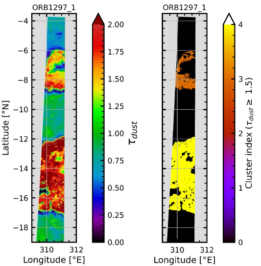
Yann Leseigneur, Thomas Gautier, Tanguy Bertrand, Aymeric Spiga, Joseph Michael Battalio, Timoté Lombard, and Luca Montabone

Dust is a crucial parameter for planetary atmospheres, particularly for Mars. These mineral micrometre-sized particles absorb and diffuse incoming sun rays, which heat the atmosphere locally. Dust also affects many atmospheric processes, such as the circulation, the water cycle, the atmospheric escape, and the CO2 cycle. In this work, we will present a novel catalogue of local dust storms on Mars. Here, we consider the following dust storm definition: a large and optically thick dust cloud [1]. The dust storms reach different stages during their lifetime: formation, growth/evolution, and dissipation/sedimentation. These storms can be classified by their spatial extension, called local storms (< 1.6 106 km2), regional storms (> 1.6 106 km2) and planetary (global) storms [2]. Questions remain about the storm formation and growth mechanisms, which are relevant to storm forecasting.

While many studies dedicated to dust storms are focused on regional storms [3, 4, 5], studying dust activity at a local scale is key to better understanding the first stages of storm formation and growth. Here, we present our work on detecting dust storms in the OMEGA/Mars Express (near-IR imaging spectrometer) dataset, chosen for its high spatial resolution (0.36-4.8 km/pixel), allowing the detection of small storms. We developed a method to detect automatically storms from dust optical depth data (see Figure 1) computed at 0.9 µm [6] available from late Martian Year 26 to mid MY 30. The storm detections have been confirmed manually and compiled into the OMEGA Dust Storm Catalogue (ODSC) [7]. This catalogue is composed of 448 storm detections, from which ~81% are local storms and ~19% regional ones.


Figure 1: 
Automatic detections of two dust storms in an OMEGA/Mars Express observation. [Left] and [right] correspond respectively to the dust optical depth map of the observation derived by [6] and the storm detection mask number. Adapted from [8].


Using this catalogue, we studied the spatial, time and diurnal distribution of the detections [8], and we present here a summary of the results. The local storm activity is widespread on Mars (see Figure 2), with favoured areas such as southern polar cap edges, flushing dust storm channels, or Hellas Planitia and Valles Marineris [8]. Most of the storm detections have been made between 10:00 and 18:00, reaching a maximum at 14:00-16:00 [8]. The storm growth mechanisms seem to be less efficient during particular periods of the Martian year, as during the northern solstitial pause (Ls ~240-270°), when we are still detecting many local storms, while the regional storm activity is low. Regional storm detections are mostly concentrated during MY 29 and MY 28, more specifically during the early formation stage of the Global Dust Storm (Ls~265-270°) [8]. This suggests that the lifting and transport processes were stronger and more effective during this period.


Figure 2: Spatial distribution of the OMEGA Dust Storm Catalogue detections [top] and OMEGA/Mars Express observations [bottom] from MY 26 to 30 without the MY 28 Global Dust Storm period (Ls~265-305°). For [top], the circles and hexagons symbolised respectively local and regional storms. Extracted from [8].

This new local and regional storm catalogue will also be useful for preparing observations of future missions such as the Martian Moons eXploration (MMX, JAXA), which will also study the Martian atmosphere [9] from 2027. Due to its equatorial orbit, MMX and its instrumental payload, especially the MMX InfraRed Spectrometer (MIRS, [10]), will give the opportunity to study diurnal variations of the storms, and therefore to constrain the storm formation and growth mechanisms. The ODSC, among other catalogues [3, 4, 5], is notably used to schedule Martian dust storm observations.

References:
[1] Kahre M. A. et al. (2017), Cambridge Univ. Press, The Atmosphere and Climate of Mars, 295-337. [2] Cantor, B. A et al. (2001) JGR, 106(E10), 23653–23687. [3] Battalio M. & Wang H. (2021) Icarus, 354, 114059. [4] Guha B. K. et al. (2024) JGR Planets, 129, e2023JE008156. [5] Lombard T. & Montabone L. (2024), 10th International Conference on Mars, abstract #3041.  [6] Leseigneur Y. and Vincendon M. (2023) Icarus, 392, 115366. [7] Leseigneur Y. et al. (2025) Zenodo, 10.5281/zenodo.17380018. [8] Leseigneur Y. et al. (2026) JGR: Planets, 131, e2025JE009502. [9] Ogohara K. et al. (2021) Earth, Plan. and Space, 74, 1. [10] Barucci M. A. et al. (2021) Earth, Plan. and Space, 73, 211.

How to cite: Leseigneur, Y., Gautier, T., Bertrand, T., Spiga, A., Battalio, J. M., Lombard, T., and Montabone, L.: Chasing the Martian Dust Storms with the OMEGA Dust Storm Catalogue, Europlanet Science Congress 2026, The Hague, The Netherlands, 7–11 Sep 2026, EPSC2026-989, https://doi.org/10.5194/epsc2026-989, 2026.

15:03–15:15
|
EPSC2026-977
|
ECP
|
On-site presentation
Guillaume Petzold, Franck Montmessin, Juan Alday, François Forget, Ehouarn Millour, and Loïc Verdier

Introduction

Dust is the main radiatively active component of the Martian atmosphere and the key driver of its thermal structure, its dynamics and thus of the water vapor distribution. Modelling the water cycle, in particular its upper atmospheric distribution, therefore relies on a dust scheme that produces a realistic representation of the dust vertical distribution in the atmosphere of Mars.

In the current Mars Planetary Climate Model (Mars PCM) [1], the dust size distribution is assumed to follow a log-normal distribution, characterized by moments . The model scheme uses two of them [2] : M0 (the number of particles) and M3 (linked to the dust mass mixing ratio). From these two moments, the dust mean radius can be determined :

However, to permit this calculation, the variance σ02 is fixed (σ0= 0.64) everywhere in the model. This is a strong limitation, as sedimentation acts more efficiently on large particles than on small ones, so the size distribution naturally becomes narrower with altitude, and the variance is thus not constant. Since small particles dominate the radiative heating at high altitudes and act as condensation nuclei for water-ice clouds, a better representation of the size distribution, and especially of its variance, is critical for the simulated atmosphere as a whole.

Methods

We overcome this limitation by introducing a third moment, with the new tracer M2, transported by the model alongside M0 and M3. M2 is initialised from the two existing moments under the log-normal assumption and is then free to evolve. With three moments, the variance is now able to vary in space and time :

The mean radius and the effective radius are now obtained directly from the transported moments, without any prescribed variance :

The new tracer is included in every process that acts on the dust distribution. Sedimentation now redistributes M0, M2 and M3 in a way that depends on the size of the particles, so that the variance naturally decreases with altitude as small particles remain high longer than large ones. The cloud microphysics scheme [3] also needs the implementation of a new condensation nuclei tracer to ensure the conservation. The dust injection scheme is also adapted to provide the three moments in a consistent way. The radiative transfer, which is sensitive to the effective variance, now sees a distribution that varies with altitude and season, rather than a fixed one.

Results

Simulations with the new three-moment scheme show several improvements compared to the two-moment reference. The simulated column dust opacity is slightly closer to the dust climatology of Montabone et al. (2015) [4], both in amplitude and in seasonal distribution. More importantly, the effective radius now decreases with altitude (Figure 1), which is the direct signature of the improved sedimentation process, while we observe the same effect on the effective variance, which is not fixed anymore. This new vertical evolution of the dust distribution impacts the radiative rates and, through it, the water cycle.

The most important result concerns water vapor at high altitudes during the dusty perihelion season. The two-moment scheme underestimates the amount of water vapor observed by ACS (Atmospheric Chemistry Suite) [5] above the lower atmosphere at this season, a long-known issue of the model. With the three-moment scheme, more water vapor reaches the upper atmosphere and the agreement with ACS profiles is significantly improved (Figure 2). The implementation doesn’t only affect the vertical distribution of water vapor, the results also feature the water vapor column-integrated distribution. First results on the D/H cycle are also presented, looking at how the new size distribution changes the fractionation between HDO and H2O through cloud microphysics and through transport to the altitudes at which water can be photodissociated.

Conclusion

Adding a third moment to the Mars PCM dust scheme is a physically motivated modification of the model that lifts the fixed variance assumption and lets the dust distribution evolve more naturally with altitude and season. It brings the simulated dust opacity and the high-altitude water vapor closer to observations, and opens a new path to study the D/H cycle and water escape in a consistent framework.

Figure 1. Zonal-mean effective radius (top) and effective variance (bottom) as a function of altitude and Ls, simulated with the three-moment scheme during MY33.

Figure 2. Alt–Ls distributions for ACS (top), PCM (middle) and their difference PCM−ACS (bottom) for MY35 with the two-moment scheme (left) and the new three-moment scheme (right)


References

[1] Forget, F., et al. (1999), Improved general circulation models of the Martian atmosphere from the surface to above 80 km, J. Geophys. Res., 104(E10), 24155–24175, doi:10.1029/1999JE001025.

[2] Madeleine, J.‐B., et al. (2011), Revisiting the radiative impact of dust on Mars using the LMD Global Climate Model, J. Geophys. Res., 116, E11010, doi:10.1029/2011JE003855.

[3] Navarro, T., et al. (2014), Global climate modeling of the Martian water cycle with improved microphysics and radiatively active water ice clouds, J. Geophys. Res. Planets, 119, 1479–1495, doi:10.1002/2013JE004550

[4] Montabone, L., et al. (2015), Eight-year climatology of dust optical depth on Mars, Icarus, Volume 251, 2015, Pages 65-95, ISSN 0019-1035, https://doi.org/10.1016/j.icarus.2014.12.034.

[5] Fedorova, A., et al. (2023). A two-Martian years survey of the water vapor saturation state on Mars based on ACS NIR/TGO occultations. Journal of Geophysical Research: Planets, 128, e2022JE007348. https://doi.org/10.1029/2022JE007348

How to cite: Petzold, G., Montmessin, F., Alday, J., Forget, F., Millour, E., and Verdier, L.: Implementing a third moment in the dust scheme of the Mars PCM : impacts on water vapor and D/H, Europlanet Science Congress 2026, The Hague, The Netherlands, 7–11 Sep 2026, EPSC2026-977, https://doi.org/10.5194/epsc2026-977, 2026.

15:15–15:27
|
EPSC2026-687
|
ECP
|
On-site presentation
Thomas Pierron and François Forget

Introduction:
The interannual variability of Martian global dust storms remains one of the major questions in Mars atmospheric science. While regional dust storms occur every year during southern spring and summer, only some Martian years exhibit planet-encircling dust storms. Several studies have proposed that this variability may be statistically correlated to Mars orbital angular momentum relative to the solar system barycenter. In particular, Shirley (2015, 2017) proposed that an inertial acceleration, referred to as the Coupling Term Acceleration (CTA), could couple the orbital motion of Mars to its proper rotation and act as a dynamical forcing on the atmosphere. Consequently, this term was used in both numerical and observational studies to investigate whether orbit-spin coupling could contribute to the timing and occurrence of Martian global dust storms (Shirley and Mischna, 2017; Mischna and Shirley, 2017; Newman et al., 2019; Shirley et al., 2020). Here, following Pierron and Forget (2026), we reassess the theoretical framework of this orbit-spin coupling hypothesis by rederiving the inertial forces acting on a parcel of air in a rotating and orbiting planetary frame.

The orbit-spin coupling hypothesis:
In Shirley (2017), the CTA was obtained from the derivation of the velocity of an atmospheric parcel expressed in an inertial frame and then transformed into rotating reference frames associated with the orbital and spin motions of the planet. The resulting acceleration was argued to contain a term proportional to (Ω × ω) × r, where Ω is the orbital angular velocity, ω is the planetary spin angular velocity, and r is the position of the air parcel relative to the planet center. Such a term would represent a direct inertial coupling between orbit and spin. Since it is proportional to the orbital angular velocity, and expressed in terms of the time variation of the orbital angular momentum, it has been hypothesized to provide a dynamical forcing depending on time, that could contribute to the initiation of Martian global dust storms.

As shown in Pierron and Forget (2026),  this term results from an inconsistent use of the transport theorem between rotating frames and should not appear in the correctly derived momentum equation.

Inertial forces and gravitational tides:
We start from the velocity of a parcel of air in the inertial frame,

V = dR/dtR0 + ω × r + v,

where R is the position of the planet center, ω is the planetary spin angular velocity, r is the parcel position relative to the planet center, and v is the parcel velocity in the planet-fixed frame. The standard transport theorem gives

dV/dtR0 = dv/dtR2 + ω × (ω × r) + 2ω × v + dω/dtR2 × r + d²R/dt²R0.

This expression contains only the classical inertial accelerations (centrifugal, Coriolis, and Euler terms). The last term is the translational acceleration of the planet along its orbit. It can be expressed as a function of the orbital angular momentum and its time derivative, but it does not involve the planetary spin and therefore is not an orbit-spin coupling term.

Moreover, this orbital inertial acceleration is not an atmospheric forcing. Applying Newton's second law to the whole planet-atmosphere system gives, to first order,

d²R/dt²R0 = g_ext(R),

therefore, for an atmospheric parcel we have

m g_ext(R + r) - m d²R/dt²R0 = m ∇g_ext(R) · r.

Thus, the orbital inertial acceleration is almost entirely compensated by the external gravitational field. The remaining term is the well known gravitational tide and not a direct orbit-spin coupling acceleration.

Implications for Martian global dust storms:
Our calculations show that the CTA should not be included in the atmospheric momentum budget of Mars general circulation models. Although true orbit-spin coupling exists through gravitational tidal torques, it acts slowly by modifying the spin rate of a planet over long timescales. It does not provide an instantaneous atmospheric forcing capable of explaining the interannual variability of Martian global dust storms. The occurrence of such storms is therefore more likely controlled by atmospheric dynamics, radiative-dust feedbacks, and the spatial and temporal variability of surface dust reservoirs (Mulholland et al., 2013; Newman and Richardson, 2015).

Figure 1: Schematic representation of the reference frames and vectors used in this study. R0 is the inertial barycentric frame, R1 rotates with the orbital angular velocity Ω, and R2 is the planet-fixed frame rotating with spin angular velocity ω. The vectors R, r, and v denote the planet position, the parcel position relative to the planet center, and the parcel velocity in R2, respectively.

References:
Shirley, J. H. (2015). Icarus, 251, 128-144.
Shirley, J. H. (2017). Planetary and Space Science, 141, 1-16.
Shirley, J. H., and Mischna, M. A. (2017). Planetary and Space Science, 139, 37-50.
Mischna, M. A., and Shirley, J. H. (2017). Planetary and Space Science, 141, 45-72.
Newman, C. E., Lee, C., Mischna, M. A., Richardson, M. I., and Shirley, J. H. (2019). Icarus, 317, 649-668.
Shirley, J. H., McKim, R. J., Battalio, J. M., and Kass, D. M. (2020). Journal of Geophysical Research: Planets, 125, e2019JE006077.
Mulholland, D. P., Read, P. L., and Lewis, S. R. (2013). Icarus, 223, 344-358.
Newman, C. E., and Richardson, M. I. (2015). Icarus, 257, 47-87.
Pierron, T., and Forget, F. (2026). Icarus, 450, 116984.

How to cite: Pierron, T. and Forget, F.: No theoretical basis for orbit–spin coupling as a forcing of Martian global dust storms, Europlanet Science Congress 2026, The Hague, The Netherlands, 7–11 Sep 2026, EPSC2026-687, https://doi.org/10.5194/epsc2026-687, 2026.

15:27–15:30

Orals THU4: Thu, 10 Sep, 16:00–17:30 | Room Neptune (Spinoza Foyer)

Other planets, Past climates, Venus atmosphere
16:00–16:15
|
EPSC2026-889
|
ECP
|
On-site presentation
Francesca Vitali, Stefania Stefani, Giuseppe Piccioni, Ha Tran, Marcel Snels, Davide Grassi, Christian Boulet, David Biondi, and Angelo Boccaccini

Our solar system’s planetary variety stems from distinct evolutionary paths that also influenced the presence of atmospheres. They represent primary determinants of planetary environments and potential habitability, making their characterization essential in both planetary and exoplanetary science.

Central to this study is having detailed spectroscopic databases, such as HITRAN [1]. Specifically, the Collision-Induced Absorption represents a critical opacity source, most of all in high-density atmospheres. Despite its importance, significant gaps remain in both experimental and theoretical CIA data. To address this, we performed new experimental measurements of H2+H2 and H2+CO2 mixtures, important for jovian, early martian, and exoplanetary atmospheres, covering previously unexplored temperature and spectral ranges.

We used an experimental setup called PASSxS which can be visualized in Figure 1.

Figure 1: A picture of the experimental setup

It consists of an atmospheric simulation chamber containing the gas or mixture of gases under investigation, which can sustain pressures up to 70 bar. It can be heated up to 550 K and cooled down to 100 K. It also contains a Multi-Pass cell, characterized by an optical path of 3.27 m, coupled with a high-resolution FT-IR spectrometer through a series of transfer optics placed in a vacuum chamber. The maximum resolution achievable is 0.002 cm-1.

For pure H2 (99.9999% purity), we measured the fundamental band of the H2 CIA between 4000 and 5500 cm-1 at a resolution of 0.05 cm-1, across seven temperatures (116- 498 K), and various densities. Fig. 2 shows the absorption coefficients measured at each considered temperature and corresponding pressures. The high resolution allowed us to resolve the so-called interference dips, visible on the blow-up of Fig. 2.

Figure 2: CIA absorption coefficients for a pure H2 gas measured at seven different temperatures

They represent a lack of absorption observed at the same spectral position as the H2 quadrupolar lines, coming from the interference phenomenon between the induced dipole moments acquired by the H2 molecules in consecutive collisions [3]. They have been previously observed in other experimental works [4-8] but only at temperatures equal to and less than 300 K. Applying the theoretical profile developed by Kelley et al. [6], we fitted the resolved interference dips at each density to retrieve the intracollisional halfwidth parameter. It exhibited a linear density dependence across all temperatures, as illustrated in Fig. 3 for the Q(1) interference dip at 4155 cm-1.

Furthermore, the integrated absorption coefficients within the spectral range of the interference dips followed a cubic trend with density.

These results provide new insights into the density-dependence of those features currently unaccounted for in existing theoretical models. A paper containing these new results is currently in preparation.

The next step will be to perform the same high-resolution measurements using a H2-He mixture to investigate the effect of He on the behavior of those features.

Figure 3: Q(1) intracollisional halfwidth as a function of the density for each investigated temperature.

In the same spectral region, new measurements of the H2+CO2 CIA have been performed. We used a total pressure of 12 bar, with 17% of volume mixing ratio (VMR) of CO2 for six temperatures, from 241 K to 498 K, at a resolution of 1 cm-1.

While room-temperature measurements have been recently reported [9-10], there is a lack of experimental data for other temperatures.

Fig. 4 shows the measured CO2-H2 CIA binary absorption coefficients for all six temperatures explored.

Figure 4: CO2-H2 CIA binary absorption coefficients

At room temperature, our experimental data have been compared with the existing experimental data, showing a good agreement. We also compared our results with semi-empirical calculations based on the approach described in [11] at each investigated temperature.

Although the theoretical band shape showed significant discrepancies with the experimental results, the integrated band intensity showed reasonable agreement. Finally, following the method employed in [12], we fitted the experimental BACs with a temperature-dependent exponential profile. This procedure allowed us to obtain a set of wavenumber-dependent coefficients that can be used to calculate the BACs at every temperature inside the investigated range. The wavenumber-dependent coefficients, along with the measured BACs, are now available on the Zenodo platform (https://doi.org/10.5281/zenodo.18327685).

These results, obtained in collaboration with Dr. Tran (LMD, Paris) and published in [13], highlight the necessity for more refined theoretical models, even if they can be used to provide a reasonable estimate of the integrated band intensity.

Future work will focus on high-resolution measurements of H2-CO2 mixtures to determine reliable H2-broadening coefficients for CO2 lines, which is so far not available at different temperatures.

Acknowledgements:  This work has been developed under the ASI-INAF agreement n. 2023-6-HH.0, and supported by the EMM (Earth Moon Mars) project of PNRR (WP 1500-13)

References

[1] Gordon I. E. et al. (2026) JQSRT, Vol. 353

[2] Terragni J. et al. (2025), JQSRT, Vol. 347

 [3] Van Kranendonk J. (1968), Canadian Journal of Physics, Vol. 46 N.10

[4] J. D. Poll et al (1975), Can. J. Phys., 53, 954

[5] A. R. McKellar et al. (1975), Can. J. Phys., 53, 2060

[6] J. D. Kelley et al. (1984), Phys. Rev. A, 29, 1168

[7] J. P. Bouanich et al. (1990), JQSRT, 44, 4

[8] J. Westberg et al. (2025), Optics Express, 33, 5

[9] W. Fakhardji et al. (2022), JQSRT, Vol. 283

[10] D. Mondelain et al. (2021), JQSRT, Vol. 260

[11] Turbet M. et al. (2020), Icarus, Vol. 346

[12] Tran H. et al. (2024), Icarus, Vol. 422 

[13] Vitali F., et al. (2026), Icarus, Vol. 455

How to cite: Vitali, F., Stefani, S., Piccioni, G., Tran, H., Snels, M., Grassi, D., Boulet, C., Biondi, D., and Boccaccini, A.: Collision-induced absorption in planetary atmospheres: present data and future perspectives, Europlanet Science Congress 2026, The Hague, The Netherlands, 7–11 Sep 2026, EPSC2026-889, https://doi.org/10.5194/epsc2026-889, 2026.

16:15–16:27
|
EPSC2026-1203
|
ECP
|
On-site presentation
Yangcheng Luo, Franck Lefèvre, and François Forget

Owing to gravitational perturbations from the giant planets, the absence of a large stabilizing moon, and its non-spherical shape, Mars could have experienced large obliquity variations over its history. Numerical simulations suggest that over the past 10 Myr, Mars’s obliquity has spanned a range of ~30°, varying between ~15° and ~45°, with the long-term mean shifting from ~35° to ~25° around 5 Myr ago and superimposed rapid oscillations of up to ~20° on ~100-kyr timescales.

High obliquity increases polar insolation, accelerating the sublimation of surface ice and thereby raising atmospheric water vapor, whereas low obliquity favors cold trapping at the poles and a much drier atmosphere. Because the photolysis products of water vapor act as key catalysts in Martian photochemistry, variations in Mars’s obliquity can strongly influence atmospheric chemistry by modulating the atmospheric water content.

We use a fully coupled 3D photochemistry–radiation–dynamics model, the Mars Planetary Climate Model (PCM), to test this hypothesis and to quantify how Martian atmospheric composition and chemistry respond to obliquity variations over the recent past. A key strength of this class of models is its ability to self-consistently simulate the spatiotemporal distribution of atmospheric water vapor through polar sublimation–condensation and 3D atmospheric transport, as well as the atmospheric CO2 abundance through the seasonal exchange of CO2 with the polar caps.

We first evaluate the capability of the model to reproduce the present-day composition of the Martian atmosphere. One-dimensional photochemical models underestimated CO by up to ~85%, a discrepancy that has persisted for more than three decades. The Mars PCM reproduces a much more realistic CO abundance, yielding a global annual mean of ~750 ppmv, close to observed values of 800–960 ppmv. We find that tuning key reaction rates or including heterogeneous chemistry on airborne dust particles can further improve agreement with observations. However, the model simultaneously predicts H2 abundances more than an order of magnitude higher than observed, transforming the long-standing CO deficit problem into an H2 surplus problem.

We then simulate the Martian atmosphere across obliquities from 10° to 45°. The results confirm the expected obliquity control on atmospheric water vapor. Near the present-day obliquity, increasing obliquity—and hence atmospheric water vapor—enhances the production of OH, a photolytic product of water vapor and a key atmospheric oxidant, thereby increasing the oxidizing capacity of the atmosphere and reducing the abundance of reduced species such as CO.

At obliquities below ~16°, extremely low polar temperatures lead to the formation of a massive CO2 polar ice cap, substantially reducing the atmospheric CO2 column. The weakened UV shielding enhances H2O photolysis, resulting in a further decline in CO as obliquity decreases.

At high obliquity, rapid H2O photolysis increases odd-hydrogen radicals by orders of magnitude, but the abundance of H2O2, which is derived from odd-hydrogen radicals, remains relatively stable, only modestly higher than present-day levels. This limits the likelihood that extremely elevated H2O2 concentrations at high obliquity would have sterilized organic matter produced by ancient life at the surface or in the shallow subsurface.

How to cite: Luo, Y., Lefèvre, F., and Forget, F.: Oscillations in the Composition and Oxidizing Capacity of the Martian Atmosphere Driven by Obliquity Variations, Europlanet Science Congress 2026, The Hague, The Netherlands, 7–11 Sep 2026, EPSC2026-1203, https://doi.org/10.5194/epsc2026-1203, 2026.

16:27–16:39
|
EPSC2026-11
|
On-site presentation
Michael Way, Eric Wolf, and Mattias Green

The Faint Young Sun Paradox posits that a modern Earth atmosphere placed on Earth in the Hadea/Archean would result in a snowball world. However, zircon data indicate that there was liquid water present at least 4.4 gigayears ago (Wilde et al. 2001). It is generally accepted that CO2 partial pressures (PP) were higher, but there are few consistent contraints on what that PP was. We use a full-complexity 3-D GCM (ROCKE-3D; Way et al. 2017) with ocean and sea ice dynamics to demonstrate that there are a wide variety of climate states possible in the Eoarchean. We see ice-free states with high CO2 PP, a variety of water belt states for medium CO2 PP, and snowball states with low CO2 PP. We also examine how the faster rotation rate of earth (shorter Length of Day) impact these climate states as well as what lower atmospheric pressures reveal given proxy data indicating pressures as low as 0.23 bar were possible in the Archean (Som et al. 2016). Studies like these not only have implications for characterizing ancient Earth's climate, but also contraining the climates of exoplanetary worlds, which we will touch upon.

Som et al. (2016) Nature Geoscience, 9, 448 http://dx.doi.org/10.1038/ngeo2713
Way et al. (2017) Astrophysical Journal Supplement Series 231:12 https://doi.org/10.3847/1538-4365/aa7a06
Wilde et al. (2001) Nature 409, 175 https://doi.org/10.1038/35051550

How to cite: Way, M., Wolf, E., and Green, M.: Exploring Earth's Eoarchean Climate in the context of the Faint Young Sun Paradox, Europlanet Science Congress 2026, The Hague, The Netherlands, 7–11 Sep 2026, EPSC2026-11, https://doi.org/10.5194/epsc2026-11, 2026.

16:39–16:51
|
EPSC2026-491
|
ECP
|
On-site presentation
Joanna Egan, Bianca Ceragioli, Maureen Cohen, James Holmes, John Plane, and Manish Patel

The atmosphere of the planet Venus contains an extensive sulfur cycle, with permanent sulfuric acid (H2SO4) clouds and haze layers spanning altitudes from 48 km to ~90 km. H2SO4 is formed from SO2 near the cloud top. Observations of SO2 in the Venusian atmosphere show concentrations of ~100 ppm below the sulfuric acid clouds and 0.1 – 1 ppb at the cloud top. Known chemistry is insufficient to produce the observed decrease in SO2 and no chemical models have successfully reproduced the three orders-of-magnitude decrease. The precise cause of the SO2 decrease remains unknown. Many chemical processes have been proposed that could contribute to the removal of SO2, including conversion to other sulfur reservoir species such as polysulfur (S2, S3, S4, S8, etc.) or polysulfur oxides (SnO); oxidative uptake to droplets by H2O2 or O3; increased uptake due to buffering of the pH of the cloud droplets by dissolved salts, and reaction with NOx species.

Two possible routes for SO2 + NOx chemistry have been postulated: reactive uptake [1] and the lead chamber process [2]. [1] reported single droplet levitation experiments which showed droplet growth only when SO2 and NO2 were both present. [2] proposed that NO and NO2 could catalyse SO2 conversion to SO3, leading to conversion to sulfuric acid by reaction with water, in a process analogous to the Lead Chamber process previously used to produce sulfuric acid for industrial use on Earth.

We present a newly developed droplet chemistry module in the Venus Planetary Climate Model, which extends the gas phase chemistry scheme to permit aqueous and droplet surface reactions. Gases condense to the cloud droplets according to their Henry’s law solubilities, and react with other species, which are then released from the droplets when they exceed their solubility limits. We use this new scheme to test both reactive uptake of SO2 and NO2 and the “lead chamber” process. In both of these cases, we predict the increases required to the reaction rates or the NOx reactant concentrations to fully explain the observed SO2 decrease through the clouds.

References:

  • Ubukata, S., et al., Uptake of SO2 into sulfuric acid droplets through the oxidation by NO2 under Venus-analogous conditions. ACS Earth and Space Chemistry, 2025. 9(6): p. 1525–1533.
  • Sill, G.T., The clouds of Venus: Sulfuric acid by the lead chamber process. Icarus, 1983. 53(1): p. 10–17.

How to cite: Egan, J., Ceragioli, B., Cohen, M., Holmes, J., Plane, J., and Patel, M.: Depletion of Venusian SO2 by liquid phase NOx chemistry, Europlanet Science Congress 2026, The Hague, The Netherlands, 7–11 Sep 2026, EPSC2026-491, https://doi.org/10.5194/epsc2026-491, 2026.

16:51–17:03
|
EPSC2026-992
|
ECP
|
On-site presentation
Gwenaël Milcareck, Gabriella Gilli, Aurelien Stolzenbach, Antoine Martinez, Alberto Mendi, and Thea Kozakis

Venus provides a unique natural laboratory for the study of rocky exoplanets close to their host stars, where intense irradiation may drive atmospheric conditions analogous to those of Venus. The population of rocky planets has grown significantly with technological advances in the detection of such bodies, and most of them have been discovered orbiting M-type stars. However, the atmospheric characteristics of this population remain an open question. In addition, the detection of Earth-like planets is a major challenge in the search for extraterrestrial life because the main characteristics of Earth-like planets are similar to those found on other terrestrial planets like Venus.


Venus and Earth are regarded as twin sisters due to the many physical characteristics they share (size, mass, density, etc.). However, the main difference lies in their atmospheres. Possible atmospheric constituents such as CO2 are now detectable with JWST [1] but most of species will be corroborated only with new generation of instruments on board the Extremely Large Telescope (ELT) (e.g. ANDES [2] or with the Large Interferometer for Exoplanets (LIFE) [3]). The study of rocky exoplanet atmospheres is strongly complicated by clouds and aerosols. Cloud layers can mask the deeper atmosphere in transmission and emission spectroscopy [4], [5], while cloudy CO₂–N₂ atmospheres may produce similar spectra for both CO₂- and N₂-dominated cases [6]. As a result, observations cannot easily distinguish between Venus-like and Earth-like planets based only on CO₂ and N₂ spectral signatures.


Thus, studying photochemistry is essential because it occurs primarily above the cloud layer, where atmospheric species remain observable. Photochemical processes can produce distinctive spectral signatures that may be detectable remotely and could therefore help distinguish between different types of planetary atmospheres, such as Venus-like and Earth-like worlds. The photochemistry of planetary atmospheres around M-type stars differs from that around the Sun due to a different stellar spectrum and thus different photolysis and photochemical reactions. [7] used 1D photochemical models to study the atmospheres of exo-Venuses orbiting K- and M-type stars. While on Venus, SO2 is heavily depleted in the cloud, on Venus-like planets receiving low UV flux (e.g. from M-dwarf colder stars) the photolysis would be inefficient to convert SO2 into H2SO4 clouds, allowing sulphur species to survive in the upper atmosphere. To date, no 3D studies have been carried out. Tidal-locked rocky planets could exhibit different spectral signatures between the solar and antisolar sides. However, the resulting atmospheric circulation on such planets could also redistribute these species and alter their abundances. Studying 3D photochemistry on Venus analogues around M-dwarf stars will enable us to narrow down the species that may be detected in the future by the JWST or the ELT.


To simulate the photochemistry of planets with physical characteristics similar to those of Venus orbiting M-dwarf stars, we used the Generic-PCM coupled with the photochemical module developed by [8]. This photochemical module is a chemical solver that tracks the evolution of chemical species linked through a network of chemical reactions and photodissociation processes. We included sulfur-bearing species as well as the main reactions involved in the production and loss of H2SO4, following the work of [9]. We adopted synthetic M-dwarf spectra from [10,11] to reproduce the photochemistry of Venus-like planets orbiting this type of star. In addition, we developed a simplified H2SO4-H2O condensation scheme to simulate the condensation of H2SO4-H2O droplets without specific microphysical processes similarly as [12]. This module includes condensation, re-evaporation and sedimentation processes with a fixed particle distribution.

We performed simulations from the surface up to 100 km altitude for Venus-like planets subjected to different M-dwarf stellar spectra. In this work, we investigated how sulfur-bearing species survive above the cloud deck at both the substellar and antistellar points, and how atmospheric circulation influences photochemistry and the spatial distribution of chemical species across the planet. We also evaluated the changes in H2O and H2SO4 production and loss between a Venus analogue orbiting an M-dwarf star and one orbiting the Sun, and finally, identified the chemical species above the cloud layer that could be detected on potential Venus-like planets.


References :

[1] Greene et al. (2023), Nature, doi:10.1038/s41586-023-05951-7

[2] Palle et al. (2023), Experimental Astronomy, doi:10.1007/s10686-025-10000-4

[3] Konrad et al. (2022), Astronomy & Astrophysics, doi:10.1051/0004-6361/202141964

[4] Ehrenreich et al. (2012), Astronomy & Astrophysics, doi:10.1051/0004-6361/201118400

[5] Lustig-Yaeger et al. (2019), The Astrophysical Journal Letters, doi:10.3847/2041-8213/ab5965

[6] Benneke et al. (2012), The Astrophysical Journal, doi :10.1088/0004-637X/753/2/100

[7] Jordan et al. (2021), The Astrophysical Journal, doi:10.3847/1538-4357/ac1d46

[8] Jaziri (2021), doi:10.70675/e18a9ce7z543dz4540zba04zea34b71ab894

[9] Stolzenbach et al. (2023), Icarus, 10.1016/j.icarus.2023.115447

[10] Rugheimer et al. (2013), Astrobiology, doi:10.1089/ast.2012.0888

[11] Rugheimer et al. (2015), The Astrophysical Journal, doi:10.1088/0004-637X/809/1/57

[12] Dai et al. (2022), Journal of Geophysical Research: Planets, doi:10.1029/2021JE007060

Acknowledgments: This work is funded by the Project CNS2024-154576 funded by MCIU/AEI, PN2024 -Research Consolidation-State Subprogram for Training, Attraction and Retention of Research and Innovation Talent - State Program of Human Resources-PEICTI 2024-2027.”

How to cite: Milcareck, G., Gilli, G., Stolzenbach, A., Martinez, A., Mendi, A., and Kozakis, T.: 3D photochemistry of Venus-like planets orbiting M-dwarf stars, Europlanet Science Congress 2026, The Hague, The Netherlands, 7–11 Sep 2026, EPSC2026-992, https://doi.org/10.5194/epsc2026-992, 2026.

17:03–17:15
|
EPSC2026-145
|
ECP
|
On-site presentation
Rafael Rianço-Silva, Pedro Machado, Clara Sousa Silva, Sergey Yurchenko, Pascal Rannou, and Giovanna Tinetti

Exoplanet atmosphere characterization heavily relies on spectroscopic data (as molecular cross-sections or high-resolution line-by-line lists). Despite efforts to obtain comprehensive molecular spectral libraries for exoplanet atmospheres, large gaps remain, particularly for larger molecules and higher frequencies at high spectral resolution (1, 2). One such key example is the methane (CH4) visible spectrum. CH4, the simplest hydrocarbon, is a crucial species for exoplanet atmosphere characterization and a possible biosignature in telluric planets (3), but whose complexity has prevented the production of high-resolution linelists at optical wavelengths (4, 5). This is due to the complexity of methane’s visible spectrum (making it computationally impossible to extract its visible linelists through quantum ab-initio calculations) and due to the relatively weak absorption strength of its optical absorption bands (requiring very long pathlengths which are not attainable in experimental set-ups on Earth). This lack of spectroscopic data hampers the exploration of CH4 atmospheric features at the optical wavelength regime, which will become increasingly relevant as upcoming instruments such as ELT-ANDES or VLT-RISTRETTO will start probing the optical reflection spectra of the atmospheres of close, temperate telluric exoplanets, in search of possible biosignatures (6, 7).


To address this spectroscopic data limitation, we aimed to use Titan as a natural spectroscopy laboratory, using its visible methane absorption bands to extract an empirical high-resolution spectrum of CH4 optical absorption (8, 9). For this, we observed Titan’s visible spectrum – dominated by CH4 absorption – at the highest spectral resolution ever with VLT-ESPRESSO (10). From this spectrum we extract a list of all present spectral lines and compare it with a stellar calibration spectrum obtained in the same night with the same instrument (to remove contaminating telluric lines) and with a solar high-resolution spectrum (to remove contaminating solar lines from Titan’s reflection spectrum). Following this analysis we are left with a set of spectral lines originating in absorption occurring on Titan’s atmosphere that is attributable to CH4 absorption.


Thus, we present here for the first time RRS-2026, an empirical, low-temperature high-resolution (R ∼ 190000) linelist of CH4 in optical wavelengths, with several thousands of previously unidentified lines. We employ this retrieved CH4 linelist to model spectroscopic products, such as templates suitable for high-resolution cross-correlation spectroscopy (HRCCS) studies - a first for CH4 in optical wavelengths. This HRCCS technique is a powerful tool to search for minor chemical compounds in exoplanet spectra, requiring accurate, high-resolution spectral linelists of the chemical species of interest in the observed wavelength range (11).


Our extracted linelist enabled us to perform the first HRCCS detection of CH4 in visible High-Resolution observations of Titan and Jupiter – which demonstrates the applicability of our CH4 linelist to a diverse set of planetary atmospheres (12). We also use the new retrieved methane linelist to explain past measurements of CH4 visible bands done in lower spectral resolutions (9, 13). This work sets the stage for the search for CH4 in exoplanet atmospheres through visible HRCCS using our empirical CH4 linelist, opening a new window to probe for this crucial chemical species in exoplanet atmospheres. This work also further showcases how Solar System observations provide useful products for exoplanet atmospheres research.


References:

1) Chubb, K., Robert, S., Sousa-Silva, C., et al. 2024, RAS Techniques and Instruments, 3, 636–690, doi: https://doi.org/10.1093/rasti/rzae039

2) Yurchenko, S., Tennyson, J., & Brogi, M. 2025, Nature Reviews Physics, 7, 645–659, doi: 10.1038/s42254-025-00839-z

3) Thompson M., et al, 2022; PNAS, doi.org/10.1073/pnas.2117933119;

4) Boudon, V., Champion, J., Gabard, T., et al. 2009, EPN, 40, 17, doi: DOI:10.1051/epn/2009601

5) Yurchenko, S., Owens, A., Kefala, K., & Tennyson, J. 2024, MNRAS, 528, 3719–3729, doi: https://doi.org/10.1093/mnras/stae148

6) Palle, E., Biazzo, K., Bolmont, E., et al. 2025, Experimental Astronomy, 59, 29, doi: https://doi.org/10.1007/s10686-025-10000-4

7) Martins, J., Santos, N., Figueira, P., & Melo, C. 2016, Orig. Life Evol. Biosph., 46, 487–498, doi: https://doi.org/10.1007/s11084-016-9493-2

8) Rianço-Silva R., et al, 2024, Planetary and Space Sciences, 240, 105836, https://doi.org/10.1016/j.pss.2023.105836

9) Karkoschka, E., & Tomasko, M. 2010, Icarus, 205, 674–694, doi:10.1016/j.icarus.2009.07.044

10) Pepe, F., Cristiani, S., Rebolo, R., et al. 2021, AA, 645, A96, doi: https://doi.org/10.1051/0004-6361/202038306

11) Snellen, I. 2025, ARAA, 63, 83, doi: https://doi.org/10.1146/annurev-astro-052622-031342

12) Irwin, P., Bowles, N., Braude, A., et al. 2019, Icarus, 321, 572–582, doi: https://doi.org/10.1016/j.icarus.2018.12.008

13) P.Giver. 1978, Journal of Quantitative Spectroscopy and Radiative Transfer, 19, 311, doi: https://doi.org/10.1016/0022-4073(78)90064-X


How to cite: Rianço-Silva, R., Machado, P., Sousa Silva, C., Yurchenko, S., Rannou, P., and Tinetti, G.: A high-resolution optical spectrum of methane (CH4) for exoplanet atmospheric science from VLT-ESPRESSO observations of Titan’s atmosphere, Europlanet Science Congress 2026, The Hague, The Netherlands, 7–11 Sep 2026, EPSC2026-145, https://doi.org/10.5194/epsc2026-145, 2026.

17:15–17:27
|
EPSC2026-654
|
On-site presentation
Miriam Rengel, Ladislav Rezac, Paul Hartogh, Christopher Jarchow, Thibault Cavalié, and Raphael Moreno
The Submillimetre Wave Instrument (SWI) onboard ESA’s JUpiter ICy moons Explorer (JUICE) mission acquired data of the Earth´s atmosphere during the Lunar-Earth Gravity Assist campaign in August 2024. These observations continued for several days after closest approach to investigate performance and test instrument behavior under in-flight conditions. SWI operates simultaneously in two frequency bands, 530–638 GHz and 1066–1286 GHz, with spectral resolution up to 107 provided by its Chirp Transform Spectrometers. During these calibration measurements, several molecular rotational transitions were detected, including those of hydrogen chloride (HCl) and hydrogen fluoride (HF).  
 
In this talk we summarize the context, calibration, and analysis of these data. Using a line-by-line radiative transfer model, we retrieved the abundances of HCl and HF and assess the associated uncertainties. The results are interpreted in the context of stratospheric halogen chemistry: HCl is the principal reservoir species of stratospheric chlorine, while HF is a reservoir species of fluorine (F).  More broadly, these observations provide an important end-to-end validation of SWI’s spectroscopic capabilities and establish a benchmark for future studies of Jupiter’s atmosphere and the exospheres of the Galilean icy moons with JUICE/SWI.
 
Acknowledgements
SWI has been designed and developed by an international consortium of institutes led by the Max Planck Institute for Solar System Research (MPS, Germany) and including the Laboratory for Studies of Radiation and Matter in Astrophysics (LERMA, France), the Space Research Centre of the Polish Academy of Sciences (CBK, Poland), Chalmers University of Technology (Sweden), the Institute of Applied Physics of the University of Bern (IAP, Switzerland), the National Institute of Information and Communications Technology (NICT, Japan) and the French Space Agency CNES with additional support from the Laboratoire d’Instrumentation et de Recherche en Astrophysique of the Observatoire de Paris (LIRA, France), the Laboratoire d’Astrophysique de Bordeaux (LAB, France), the RPG Radiometer Physics GmbH (Germany), and Omnisys Instrument AV (Sweden). This development has been supported by national funding agencies and other organizations, including the Deutsches Zentrum für Luft- und Raumfahrt (DLR) and by central resources of the Max-Planck-Society. R. Moreno, and T. Cavalié acknowledge funding from the Centre National d’Études Spatiales (CNES).  Juice is a mission under ESA leadership with contributions from its Member States, NASA, JAXA, and the Israel Space Agency. It is the first Large-class mission in ESA’s Cosmic Vision Program.

How to cite: Rengel, M., Rezac, L., Hartogh, P., Jarchow, C., Cavalié, T., and Moreno, R.: JUICE/SWI measurements of HF and HCl in Earth’s Atmosphere during the Lunar Earth Gravity Assist, Europlanet Science Congress 2026, The Hague, The Netherlands, 7–11 Sep 2026, EPSC2026-654, https://doi.org/10.5194/epsc2026-654, 2026.

17:27–17:30

Posters: Tue, 8 Sep, 18:00–19:30 | Foyer 2

Display time: Tue, 8 Sep, 08:30–19:30
F2.22
|
EPSC2026-30
|
ECP
|
On-site presentation
Reiichi Sato, Hiroki Karyu, Takeshi Kuroda, Yuki Nakamura, Shungo Koyama, John Plane, and Naoki Terada

The thermal structure and water cycle in the lower atmosphere of Mars are thought to be controlled by dust particles supplied from the surface, acting as cloud condensation nuclei (CCN) for water ice clouds. However, the presence of water ice clouds in the mesosphere (Bernal et al., 2021) suggests that additional CCN sources may be required. Meteoric smoke particles (MSPs) are thought to be these sources, which are composed of carbonates formed by the reaction of atmospheric molecules with metal atoms ablated from meteoroids as they enter the atmosphere (Plane et al., 2018).

Due to their small size and difficulty in observing them, the distribution and function of MSPs as CCN remain unclear. Previous model studies have investigated cloud formation associated with MSPs (Hartwick et al., 2019). However, due to computational constraints in the GCM, these studies assumed that MSPs are supplied only from the upper boundary of the model, located at approximately 60 km altitude. As a result, they could not explicitly represent the 60–100 km altitude region, where meteoric metal ablation and subsequent chemical reactions responsible for MSP formation are expected to occur.

Here we focus on meteoric Mg species commonly observed in the Martian atmosphere (Crismani et al., 2023) and investigate their role in mesospheric cloud formation using two 1-D models: a photochemical model, PROTEUS (Nakamura et al., 2023), to evaluate the formation process of MSPs, and a cloud microphysics model, SPECK (Karyu et al., 2025), to track the evolution of the particle size distribution.

Clouds formed when CCN was supplied according to the altitude distribution of carbonates calculated by PROTEUS, but no clouds formed when CCN was supplied only from the upper boundary at an altitude of 200 km. This implies that nm-sized MSPs are not subject to sedimentation effects and that it is important to track the chemical reactions involved in the formation of MSPs.

These results support MSPs as effective condensation nuclei for Martian mesospheric water ice clouds and provide a quantitative link between meteoric metal chemistry and cloud microphysics.

How to cite: Sato, R., Karyu, H., Kuroda, T., Nakamura, Y., Koyama, S., Plane, J., and Terada, N.: Impact of meteoric smoke particles on mesospheric water ice clouds on Mars, Europlanet Science Congress 2026, The Hague, The Netherlands, 7–11 Sep 2026, EPSC2026-30, https://doi.org/10.5194/epsc2026-30, 2026.

F2.23
|
EPSC2026-74
|
ECP
|
On-site presentation
Joonas Leino, Ari-Matti Harri, Robert John Wilson, Tanguy Bertrand, and Terhi Mäkinen

Atmospheric pressure is a key indicator of weather patterns on both Earth and Mars. Variations in pressure can reveal the movement of air masses, the development of storms, and the behavior of large-scale atmospheric systems. One important type of such systems is the baroclinic wave, which forms in the presence of strong temperature gradients between the poles and the equator. These waves play a major role in redistributing heat and energy across a planet and are closely linked to storm activity. On Mars, baroclinic waves generate recurring pressure disturbances detectable by surface instruments. Leino et al. (2026) analyzed oscillations with periods of 2 to 10 sols across all available surface pressure observations. Here, we compare surface pressure oscillations derived from a General Circulation Model (GCM), specifically the Mars Planetary Climate Model (PCM), with the observations reported in Leino et al. (2026) using similar approach, and examine global pressure wave structures in both hemispheres.

Northern hemisphere midlatitude surface pressure waves in the PCM simulation intensify around Ls 170° in Mars Year (MY) 36. Eastward-propagating eddies with zonal wavenumber 2 dominate until Ls 225°, after which wavenumber 1 strengthens while overall amplitudes slightly weaken. After Ls 300°, amplitudes begin to intensify again, and the dominant structure alternates between wavenumbers 1-3.

Comparison with surface observations from Viking Lander 1 and 2 (VL1 and VL2), Perseverance, InSight, and the Mars Science Laboratory (MSL) shows partial agreement but also notable discrepancies. A major discrepancy is the absence of short-period (2-4 sol) wave peaks across all lander locations during Ls 220°-315°. However, some weaker background activity is still detected at the VL1 and VL2 sites. Observations clearly indicate a strong presence of these waves, including distinct peaks, during this period, whereas the PCM does not reproduce them. Instead, longer-period waves (5-8 sols) dominate in the model. The seasonal evolution of these waves is broadly consistent with observations, but their amplitudes are typically overestimated in the PCM.

Around Ls 330°-350°, the PCM produces a strong wave with a period of 2-3 sols. Elevated springtime amplitudes have also been observed at surface platforms during several MYs (Leino et al., 2026), although the observed pressure waves are generally weaker. In the PCM, this wave exhibit a midlatitude zonal wavenumber 3 structure and eastward propagation with a phase speed of approximately 15-20 m/s.

Despite similar latitudes, differences are found between VL1 and Perseverance: the springtime wavenumber 3 structure extends farther meridionally at VL1, while around Ls 270° the dominant wavenumber 1 structure shows a comparable meridional extent at both locations.

Southern hemisphere midlatitude waves are substantially weaker and develop around Ls 350°, with intermittent variability. Their structure is typically dominated by wavenumbers 2-3, with peak amplitudes at Ls 170°-210°, when northern hemisphere waves also begin to develop.


References

Leino, J., Harri, A.M., Wilson, R.J., Bertrand, T., Banfield, D., Mäkinen, T., Paton, M., Savijärvi, H., Martínez, G., Rodríguez-Manfredi, J.A., 2026. Baroclinic pressure oscillations in the martian atmosphere from surface observations. Icarus 456, 117138.

How to cite: Leino, J., Harri, A.-M., Wilson, R. J., Bertrand, T., and Mäkinen, T.: Modeling Baroclinic Pressure Oscillations in the Martian Atmosphere, Europlanet Science Congress 2026, The Hague, The Netherlands, 7–11 Sep 2026, EPSC2026-74, https://doi.org/10.5194/epsc2026-74, 2026.

F2.24
|
EPSC2026-188
|
ECP
|
On-site presentation
Kazuto Kashiwakura, Shohei Aoki, Sara Faggi, Geronimo Villanueva, Giuliano Liuzzi, Hideo Sagawa, and Takeshi Imamura

The D/H ratio in the Martian atmosphere is a key tracer for understanding the present-day water cycle on Mars and its broader connection to long-term atmospheric evolution. Because deuterium is less efficiently lost to space than hydrogen, the atmospheric D/H ratio has long been used to constrain the history of water loss from Mars [e.g., 1]. At the same time, the spatial and seasonal variability of D/H in the lower atmosphere is expected to reflect ongoing water-cycle processes, including exchange with surface and polar reservoirs, formation of water ice clouds, and potential subsurface-atmosphere interactions associated with condensation and sublimation of water. Characterizing the present-day distribution of D/H is therefore important not only for understanding the evolution of Martian water, but also for identifying the physical processes that control the current Martian water cycle.


Previous observations have shown that Martian water vapor is typically enriched in deuterium to about 5 VSMOW, and that its D/H ratio varies substantially in space and time [e.g., 1–5]. Additional infrared observations have shown that HDO/H2O varies with season and altitude, suggesting that the D/H distribution is influenced by water transport, cloud-related fractionation, and exchange with surface and polar reservoirs [3–7]. In particular, Villanueva et al. (2015) [2] reported strong local variability across the Martian disk from ground-based mapping. Their results suggest that water released from the north polar cap may have a representative D/H value of about 7 VSMOW, while some basins and low-lying regions show even higher enrichment and high-altitude regions show much lower values of about 1–3 VSMOW. However, these observed spatial variations cannot be explained solely by simple fractionation associated with phase changes, and their underlying mechanisms remain unclear.


In this study, we investigate the spatial and seasonal variability of D/H in the lower Martian atmosphere, with the objective of clarifying the processes responsible for the observed isotopic variations. We use ground-based high-resolution spectroscopic observations of Mars obtained with iSHELL on the NASA Infrared Telescope Facility (IRTF). IRTF/iSHELL enables spatially resolved high-resolution spectroscopy of the Martian disk, allowing simultaneous retrievals of H2O and HDO. We have obtained disk-resolved Mars observations with IRTF/iSHELL over approximately three years, covering multiple seasons and viewing geometries [8,9]. This long-term data set, combined with disk-resolved two-dimensional mapping, allows us to expand the D/H measurements across multiple times and locations and to assess whether the regional D/H variability suggested by previous studies varies with season and location. These measurements are expected to constrain isotopic fractionation processes and contribute to a more accurate understanding of the present-day Martian water cycle.


As the first step, we are currently analyzing the initial data set acquired in September 2020. This analysis focuses on deriving spatially resolved HDO, H2O, and D/H maps from the iSHELL spectra. We retrieve H2O and HDO abundances by fitting the observed spectra with radiative-transfer calculations using the Planetary Spectrum Generator (PSG), including telluric absorption, solar Fraunhofer lines, and Martian atmospheric absorption. The molecular absorption strengths are scaled relative to the CO2 absorption, which provides a reference for deriving the H2O and HDO abundances. By the time of the presentation, we plan to report the first results from the September 2020 data set, including the disk-resolved D/H map and its latitudinal profile. These results will provide an initial basis for assessing whether lower-atmospheric D/H variability is controlled by seasonal and regional factors in the active Martian water cycle.

[1] Owen et al. 1988, Science, 240, 1767.

[2] Villanueva et al. 2015, Science, 348, 218.

[3] Aoki et al. 2015, Icarus, 260, 7.

[4] Encrenaz et al. 2018, A&A, 612, A112.

[5] Alday et al. 2024, MNRAS, 530, 2919.

[6] Villanueva et al. 2021, Science Advances, 7, eabc8843.

[7] Alday et al. 2021, Nature Astronomy, 5, 943.

[8] Aoki et al. 2024, The Planetary Science Journal, 5, 158.

[9] Faggi et al. 2025, Journal of Geophysical Research: Planets, 130, e2025JE009105.

How to cite: Kashiwakura, K., Aoki, S., Faggi, S., Villanueva, G., Liuzzi, G., Sagawa, H., and Imamura, T.: Spatially resolved measurements of the D/H ratio in the lower Martian atmosphere with IRTF/iSHELL: preliminary results from 2020 observations, Europlanet Science Congress 2026, The Hague, The Netherlands, 7–11 Sep 2026, EPSC2026-188, https://doi.org/10.5194/epsc2026-188, 2026.

F2.25
|
EPSC2026-249
|
On-site presentation
Alexander Kutepov, Alexander Medvedev, Ladislav Rezac, and Artem Feofilov

The Martian mesosphere and thermosphere form a highly variable transition region coupling the lower atmosphere to the space environment. The thermal structure and circulation in this region are controlled by a delicate balance between radiative heating and cooling, gravity-wave forcing, large-scale transport, and solar forcing. Among these processes, non-LTE infrared cooling in the CO₂ 15 µm bands and solar heating by near-IR CO₂ absorption bands dominate the radiative energy budget over a broad altitude range. However, substantial uncertainty remains in quantifying collisional CO₂–O vibrational quenching processes that control these mechanisms in the Martian general circulation models (MGCMs).

In this study, we investigate the sensitivity of the Martian upper-atmosphere energy budget and dynamics to the CO₂–O quenching rate coefficient using the MAOAM MGCM (Medvedev et al, 2015). The calculations employ a modified version of the terrestrial non-LTE CO₂ radiative routine developed by Kutepov & Feofilov (2024). The routine was extended to include additional CO₂ isotopes, vibrational levels, and radiative bands in the 1–15 µm spectral region, allowing simultaneous treatment of daytime and night-time non-LTE CO₂ cooling and solar heating processes under Martian conditions.

The simulations were performed using the laboratory-supported CO₂–O quenching rate coefficient k=1.5×10⁻¹² cm3 s−1.

This value is half the size of the k=3.0×10⁻¹² cm3 s−1 coefficient currently adopted in essentially all existing Martian GCM non-LTE parameterizations, despite the absence of compelling laboratory or theoretical evidence supporting the larger value.

Our calculations demonstrate that both CO₂ 15 µm cooling and solar heating by absorption in the 1.0–2.7 µm CO₂ bands are approximately proportional to the adopted quenching coefficient. As a consequence, replacing the commonly used value by the laboratory-supported coefficient produces a dramatic reduction of both cooling and heating rates, reaching ~100–150 K sol⁻¹ in the 110–150 km altitude region. These changes modify the mean thermal structure and circulation, with variability affected the most. The results imply that the radiative energy balance and dynamical variability predicted by present-day MGCMs may be systematically biased. The results also have important implications for interpretation of stellar and solar occultation observations and for model–observation comparisons in the Martian upper atmosphere.

References

Kutepov, A. and Feofilov, A.: New routine NLTE15µmCool-E v1.0 for calculating the non-local thermodynamic equilibrium (non-LTE) CO2 15 µm cooling in general circulation models (GCMs) of Earth's atmosphere, Geosci. Model Dev., 17, 5331–5347, https://doi.org/10.5194/gmd-17-5331-2024, 2024.

Medvedev, A. S., F. González-Galindo, E. Yiğit, A. G. Feofilov, F. Forget, and P. Hartogh, Cooling of the Martian thermosphere by CO2 radiation and gravity waves: An intercomparison study with two general circulation models, Journal of Geophysical Research: Planets, 120, 913–927, doi:10.1002/ 2015JE004802, 2015.

How to cite: Kutepov, A., Medvedev, A., Rezac, L., and Feofilov, A.: The CO₂–O Quenching Rate as a Controlling Parameter of the Martian Upper-Atmosphere Energy Budget and Dynamics, Europlanet Science Congress 2026, The Hague, The Netherlands, 7–11 Sep 2026, EPSC2026-249, https://doi.org/10.5194/epsc2026-249, 2026.

F2.26
|
EPSC2026-274
|
ECP
|
On-site presentation
Yo Kawamura, Tatsuya Yoshida, Jean-Yves Chaufray, Yuki Nakamura, Naoki Terada, François Leblanc, Shungo Koyama, and Yassin Jaziri
Terrestrial planets currently in the habitable zone around M dwarfs are primary targets for exoplanet characterization. Because the pre-main-sequence phase of M dwarfs can last up to about 1 Gyr, such planets are expected to have undergone a prolonged runaway greenhouse (RG) phase, during which surface water is entirely evaporated to form an H₂O-dominated atmosphere (e.g., Kasting 1988; Ramirez & Kaltenegger 2014; Luger & Barnes 2015). H₂O photolysis followed by hydrodynamic hydrogen escape, driven by stellar X-ray and extreme-ultraviolet (XUV) heating, then results in significant planetary water loss over this prolonged phase (e.g., Kasting & Pollack 1983; Johnstone 2020; Yoshida et al. 2022).
The behavior of the oxygen produced by H₂O photolysis affects water loss. If the hydrogen outflow is sufficiently intense, oxygen can be dragged to space along with hydrogen, but the oxygen mass loading lowers the hydrodynamic escape efficiency and thereby slows water loss (e.g., Hunten et al. 1987; Guo 2019; Johnstone 2020). Otherwise, the oxygen left behind forms an O₂-accumulated atmosphere, which can limit the upward diffusive supply of hydrogen to the escape region and thereby slow water loss (e.g., Hunten 1973; Luger & Barnes 2015). Such abiotic O₂ accumulation also bears on the discussion of exoplanet habitability because the resulting oxidizing environment can hinder prebiotic chemistry (e.g., Schlesinger & Miller 1983) and may produce false positives for life (e.g., Wordsworth & Pierrehumbert 2014; Meadows et al. 2018). The behavior of oxygen during the RG phase is therefore central to understanding the habitability of terrestrial planets currently in the habitable zone around M dwarfs.
However, the feedback of the retained oxygen on water loss and habitability remains poorly understood. Kawamura et al. (2024) showed that UV shielding by O₂ retained in the atmosphere reduces the water loss rate. Such chemically mediated feedback can in turn modify both the water loss process and the formation of O₂-accumulated atmospheres. Yet such feedback remains unresolved in existing hydrodynamic escape models, which are confined to the upper atmosphere and treat neither lower-atmosphere chemistry and diffusion nor the long-term evolution of the RG phase.
Building on the 1D photochemical model of Kawamura et al. (2024), we develop a new 1D hydrodynamic escape model for an H₂O-dominated atmosphere on an Earth-like planet orbiting an M dwarf. The model extends from the thermosphere down to the surface and couples atmospheric dynamics, photochemistry, molecular and eddy diffusion, and radiative transfer, allowing us to track the transport of H- and O-bearing species under both diffusive separation and hydrodynamic outflow.
The bulk atmospheric motion is calculated by solving the 1D hydrodynamic equations for mass, momentum, and energy, following the framework of Johnstone et al. (2018). The energy equation includes stellar XUV heating, chemical heating and cooling, thermal conduction, and radiative cooling by H₂O and chemical products such as OH, treated following Yoshida et al. (2022). We adopt the H- and O-bearing chemical network of Chaffin et al. (2017), as in Kawamura et al. (2024), and calculate photolysis rates using the stellar UV spectrum of TRAPPIST-1 (Wilson et al. 2021).
To integrate the coupled advection–diffusion–chemistry continuity equation over the runaway greenhouse phase, we use a semi-IMEX Runge–Kutta scheme (Ding 2025), treating advective transport explicitly and stiff diffusion and chemical terms implicitly. The equation is solved with the “modified pass flow” algorithm, following Chaufray et al. (2024), to improve numerical stability and efficiency. We assume the runaway greenhouse phase to last 1 Gyr (Ramirez & Kaltenegger 2014). Using this model, we quantify how the retained oxygen feeds back on water loss and shapes the post-RG atmospheric composition of terrestrial planets around M dwarfs, with implications for their habitability.

How to cite: Kawamura, Y., Yoshida, T., Chaufray, J.-Y., Nakamura, Y., Terada, N., Leblanc, F., Koyama, S., and Jaziri, Y.: Oxygen feedback on water loss during the runaway greenhouse phase on terrestrial planets around M dwarfs, Europlanet Science Congress 2026, The Hague, The Netherlands, 7–11 Sep 2026, EPSC2026-274, https://doi.org/10.5194/epsc2026-274, 2026.

F2.27
|
EPSC2026-305
|
ECP
|
On-site presentation
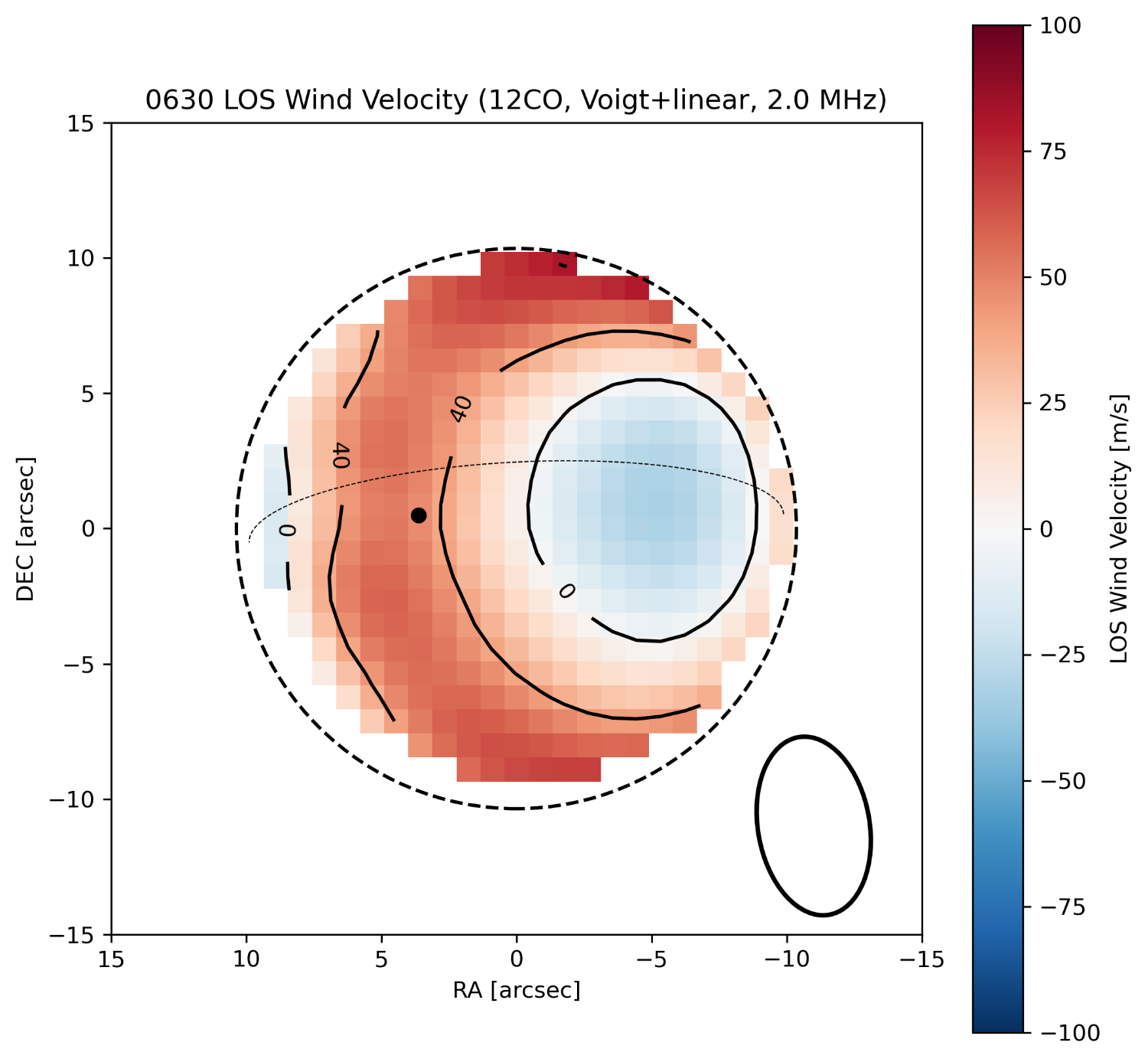
Nozomi Kakinuma, Shohei Aoki, Hideo Sagawa, Eric Villard, Kazi Rygl, Geronimo Villanueva, Sara Faggi, Frank Daerden, Séverine Robert, and Takeshi Imamura

One of the most significant features of the Martian atmosphere is the presence of dust. Dust particles are constantly suspended in the atmosphere and absorb the solar radiation, heating the lower and middle atmosphere. Therefore, dust plays an important role in determining the thermal structure of the Martian atmosphere. When strongly enhanced dust lifted from the surface covers the entire planet, the event is called a “Global Dust Storm (GDS)”. Such extreme condition can have a large influence on atmospheric circulation and material transport processes.

Wind fields during the GDS have been inferred indirectly through data assimilation using observed temperature fields (Asumi et al., 2026). However, due to observational limitations, direct measurements of the wind velocities remain scarce, and the structure of the atmospheric circulation during GDS has not been revealed. Miyamoto et al. (2021) directly measured the zonal winds around 80 km altitude in equatorial regions during the Mars Year (MY) 34 GDS by infrared heterodyne spectroscopy, but the spatial coverage was limited. In addition, the observed strong retrograde winds in the decay phase of GDS were not reproduced in the Mars global circulation model. This discrepancy implies the need for additional observational datasets to improve our understanding of Martian atmospheric circulation.

This study aims to directly determine the global wind fields during and after the MY34 GDS using data from the Atacama Compact Array (ACA) within the Atacama Large Millimeter/submillimeter Array (ALMA). ACA provides high spectral and spatial resolution, which enables to derive the global wind fields. It observed the absorption lines of 12CO and 13CO around 200 GHz, which are sensitive to higher (50-70 km) and lower (30-40 km) altitudes, respectively. The line-of-sight wind velocities of 12CO and 13CO were derived by the Doppler shift technique. Results for June 30, 2018 are shown in Figures 1 and 2.

Comparisons between ALMA observations and the GEM-Mars model’s predictions will also be presented. Several GEM-Mars simulations constrained by ALMA observations will be performed to identify the physical processes governing the observed wind fields.

Figure 1: Global wind field on June 30, 2018 derived from 12CO absorption line. Line-of-sight velocity is taken as positive. The black circle shows the beam size.

Figure 2: Same as Figure 1, but global wind fields derived from 13CO absorption line.

References

[1] Asumi, A., Sato, K., & Hayashi, Y.-Y. (2026). Effects of global dust storm in MY28 and roles of unresolved waves on the general circulation of Mars. Journal of Geophysical Research: Planets, 131, e2025JE009200. https://doi.org/10.1029/2025JE009200


[2] Miyamoto, A., Nakagawa, H., Kuroda, T., Takami, K., Murata, I., Medvedev, A. S., et al. (2021). Intense zonal wind in the Martian mesosphere during the 2018 planet-encircling dust event observed by ground-based infrared heterodyne spectroscopy. Geophysical Research Letters, 48, e2021GL092413. https://doi.org/10.1029/2021GL092413

How to cite: Kakinuma, N., Aoki, S., Sagawa, H., Villard, E., Rygl, K., Villanueva, G., Faggi, S., Daerden, F., Robert, S., and Imamura, T.: Global map of wind in Mars during and after the MY34 Global Dust Storm observed by ALMA, Europlanet Science Congress 2026, The Hague, The Netherlands, 7–11 Sep 2026, EPSC2026-305, https://doi.org/10.5194/epsc2026-305, 2026.

F2.28
|
EPSC2026-367
|
On-site presentation
Ian Thomas, Loïc Trompet, Yannick Willame, François Hendrick, Shohei Aoki, Bojan Ristic, Ann Carine Vandaele, Frank Daerden, Lori Neary, Séverine Robert, Miguel Angel López-Valverde, Jon Mason, Manish Patel, Fabrizio Oliva, and Giancarlo Bellucci and the NOMAD Team

The science phase of the ExoMars Trace Gas Orbiter (TGO) mission began on 21st April 2018, and since then the NOMAD suite of 3 spectrometers [1] has acquired around 100 million spectra, primarily of the Martian atmosphere and surface. These cover ultraviolet-visible and infrared wavelengths with different observation geometries. The 3 spectrometers are:

1) Solar Occultation (SO): 2.2-4.3 µm (2,300-4,600 cm-1), spectral resolution 0.1-0.23 cm-1 [2].

2) Limb, Nadir and Occultation (LNO): 2.2-3.8 µm (2,600-4,600 cm-1), spectral resolution 0.15-0.28 cm-1 [2], operating primarily in nadir viewing mode.

3) Ultraviolet-Visible (UVIS): 200-650 nm (15,000-50,000 cm-1), spectral resolution 1.2-1.7 nm [3], operating in solar occultation, nadir and limb viewing modes.


Together, the spectrometers are able to map the vertical distributions and/or column densities (where appropriate) of many properties and constituents of the Martian atmosphere, including H2O [4] and HDO [5], CO [6], O3 [7], HCl [8], dust/aerosol particle size [9], CO2 and H2O clouds [10], CO2 temperature and pressure [11], dayglow [12] and nightglow [13] emissions, surface ice/frost [14], plus the reflectance properties of Phobos and Deimos [15]. Also, stringent detection limits can be placed on other gases that have not yet been detected, e.g. CH4 [16].


Calibrated NOMAD spectra and derived climatologies are available to the scientific community in multiple sources, for example: the ESA Planetary Science Archive, Europlanet’s VESPA portal, and many online authors’ repositories. Likewise, modelling tools (for example the NASA Goddard Planetary Spectrum Generator), calibration routines, observation planning information and nadir footprints exist online, are available in journal articles, or can be found on the NOMAD website at nomad.aeronomie.be.


Work is ongoing to consolidate all the available datasets and tools, including python code to find and plot online datasets, forward-model the SO and LNO spectrometers, and to understand the instrument and associated uncertainties, which we will describe here. Also, documentation regarding recent calibration improvements will be highlighted and made available online for the community.


References

[1] Vandaele, A.C., et al; NOMAD, an integrated suite of three spectrometers for the ExoMars Trace Gas mission: technical description, science objectives and expected performance. (2018) Space Sc. Rev. 214, 80. https://doi.org/10.1007/s11214-018-0517-2

[2] Liuzzi G., et al; Methane on Mars: New insights into the sensitivity of CH4 with the NOMAD/ExoMars spectrometer through its first in-flight calibration. (2019) Icarus 321, 671-690. https://doi.org/10.1016/j.icarus.2018.09.021

[3] Willame, Y., et al; Calibration of the NOMAD-UVIS data. (2022) Planet. Space Sci., 218, 105504. https://doi.org/10.1016/j.pss.2022.105504

[4] Hendrick, F., et al; New Climatology of Martian Water Vapor Column Abundance Derived from NOMAD LNO Nadir Observations Over Martian Years 34–38. (2026) J. Geophys. Res. Planets. https://doi.org/10.1029/2025JE009592  

[5] Villanueva, G., et al; The deuterium isotopic ratio of water released from the Martian caps as measured with TGO/NOMAD. (2022) Geophys. Res. Lett., 49(12). https://doi.org/10.1029/2022GL098161

[6] Modak, A., et al; Martian Atmospheric CO Vertical Profiles From NOMAD Observations During the First Year of TGO Operations. (2023) J. Geophys. Res. Planets. https://doi.org/10.1029/2022JE007282

[7] Mason, J. P., et al; Climatology and Diurnal Variation of Ozone Column Abundances for 2.5 Mars Years as Measured by the NOMAD-UVIS Spectrometer. (2024) J. Geophys. Res. Planets. https://doi.org/10.1029/2023JE008270

[8] Aoki S., et al; Annual appearance of hydrogen chloride on Mars and a striking similarity with the water vapor vertical distribution observed by TGO/NOMAD. (2021) Geophys. Res. Letters 48(11). https://doi.org/10.1029/2021gl092506

[9] Flimon, Z., et al; Aerosol Climatology on Mars as Observed by NOMAD UVIS on ExoMars TGO in Journal of Geophysical Research: Planets.  (2025) J. Geophys. Res. Planets. https://doi.org/10.1029/2024JE008303

[10] Liuzzi, G., et al; First Detection and Thermal Characterization of Terminator CO2 Ice Clouds with ExoMars/NOMAD. (2021) Geophys. Res. Letters 48(2). https://doi.org/10.1029/2021gl095895

[11] Trompet, L., et al; Carbon dioxide retrievals from NOMAD-SO on ESA’s ExoMars Trace Gas Orbiter and temperature profiles retrievals with the hydrostatic equilibrium equation. II. Temperature variabilities in the mesosphere at Mars terminator. (2023) J. Geophys. Res. Planets. https://doi.org/10.1029/2022JE007279

[12] Soret, L., et al; The Martian oxygen green line dayglow: response to solar activity. (2025) Icarus. https://doi.org/10.1016/j.icarus.2025.116707

[13] Gérard, J.-C., et al; Observation of the Mars O2 visible nightglow by the NOMAD spectrometer onboard the Trace Gas Orbiter. (2023) Nature Astron. https://doi.org/10.1038/s41550-023-02104-8

[14] Valantinas, A., et al; Evidence for transient morning water frost deposits on the Tharsis volcanoes of Mars. (2024) Nature Geoscience. https://doi.org/10.1038/s41561-024-01457-7

[15] Mason, J. P., et al; Ultraviolet and Visible Reflectance Spectra of Phobos and Deimos as Measured by the ExoMars-TGO/NOMAD-UVIS Spectrometer. (2023) J. Geophys. Res. Planets. https://doi.org/10.1029/2023JE008002

[16] Knutsen, E.W., et al; Comprehensive Investigation of Mars Methane and Organics with ExoMars/NOMAD. (2021) Icarus 257. https://doi.org/10.1016/j.icarus.2020.114266

How to cite: Thomas, I., Trompet, L., Willame, Y., Hendrick, F., Aoki, S., Ristic, B., Vandaele, A. C., Daerden, F., Neary, L., Robert, S., López-Valverde, M. A., Mason, J., Patel, M., Oliva, F., and Bellucci, G. and the NOMAD Team: Publicly Available Derived Datasets and Tools for Working with Calibrated Spectra from NOMAD on the ExoMars Trace Gas Orbiter, Europlanet Science Congress 2026, The Hague, The Netherlands, 7–11 Sep 2026, EPSC2026-367, https://doi.org/10.5194/epsc2026-367, 2026.

F2.29
|
EPSC2026-598
|
ECP
|
On-site presentation
Rodrigo Zamudio Ramírez, José Guadalupe de la Rosa Canales, Paola Molina Sevilla, Jorge Cruz Castañeda, and Nigel J. Mason

1. Introduction

The photochemistry in Titan’s atmosphere begins with the dissociation and ionization of its main atmospheric constituents N2 and CH4, therefore, the nitrogen chemistry, aerosol formation, and atmospheric loss energy sources are driven from external energy sources such as Solar UV, Saturn´s magnetosphere, solar wind and galactic cosmic rays [1].

Cosmic particles, composed mainly of protons and α particles, possess a higher penetration power, which makes cosmic‑ray radiation the main mechanism responsible for ionizing Titan’s lower atmosphere [2]. For this reason, studying its effect on Titan’s atmosphere is of great importance, especially because the connection between Titan’s surface and atmosphere is unique in our Solar System: atmospheric chemistry produces materials that are deposited onto the surface and subsequently modified by surface–atmosphere interactions [3].

2. Experimental Methods

2. 1. Preparation of Titan simulated atmosphere.

The gas mixture (10% methane in nitrogen) used to simulate Titan’s atmosphere was prepared using a gas‑blending system (Figure 1) located at the Instituto de Ciencias Nucleares, Universidad Nacional Autónoma de México (UNAM). For this purpose, high‑purity gases supplied by Linde were used (N₂ = 4.8 and CH₄ = 3.7).

The gas‑blending system is a Linde FM 4660 model equipped with eight channels, each fitted with its corresponding mass‑flow controller. These controllers provide a maximum flow rate of 20 mL min⁻¹ and a minimum of 2 mL min⁻¹, allowing precise regulation of the gas flows and, consequently, the required proportions for simulating Titan’s atmosphere.

Likewise, this gas‑blending unit is connected to a high‑vacuum system, which allows the system to reach pressures below 2 × 10⁻³ mbar.

Once prepared, the gas mixture was allowed to equilibrate inside the gas containers for at least 24 hours to ensure proper homogenization. Subsequently, the reactors each with an average internal volume of 1.16 ± 0.04 L were connected to the vacuum line, and their interiors were evacuated to a pressure of 2.4 × 10⁻² mbar before introducing the gas mixture. After filling, an internal pressure of 1000 mbar was reached, corresponding approximately to the atmospheric pressure at an altitude of 10 km above Titan’s surface, where cosmic rays are expected to have a stronger effect. Once this pressure was reached, the reactors were sealed.

Figure 1. Diagram illustrating the system used for the preparation of the simulated Titan atmosphere, as well as the filling of the reactors through the vacuum line. Provided by M.C. José de la Rosa Canales, personal communication.


2. 2. Irradiation system.

The irradiation was carried out in the Unidad de Irradiación, Instituto de Ciencias Nucleares, UNAM, which is equipped with a Gammabeam 651PT deep‑pool irradiator, where the simulated atmosphere was exposed to different levels of accumulated gamma‑radiation dose, generated by 60Co sources.

2. 3. Analysis system.

The analysis after irradiation was performed using the coupled analytical technique of Gas Chromatography–Mass Spectrometry (GC–MS), which allows the separation, identification, and quantification of the compounds generated. Each analysis began at 50 °C with a five‑minute isothermal hold, followed by a temperature ramp of 10 °C min⁻¹ until reaching a final temperature of 240 °C. These conditions were maintained until the end of the run, resulting in a total analysis time of 30 minutes.


3. Results and discussion

3. 1. Identification of the Compound

The chromatograms revealed the formation of a total of seven compounds (Figure 2). The analyses indicated that all the products generated were saturated hydrocarbons (linear and branched), including ethane, propane, butane, and isobutane, which exhibited the highest response in the coupled analytical system.

The identification of these compounds was carried out by comparing their mass spectra with those from reference libraries and by injecting analytical standards.

Figure 2. Separation by gas chromatography of the compounds produced after irradiating at 483 kGy a mixture of methane (10%) in nitrogen at 298 K and a pressure of 1000 mbar. Peaks: 1 = nitrogen; 2 = methane; 3 = ethane; 4 = propane; 5 = isobutane; 6 = butane; 7 = 2‑methylbutane; 8 = 2,2‑dimethylbutane; and 9 = 2,3‑dimethylbutane.


3.2. Determination of Hydrocarbon Production Rate as a Function of Energy Dose

The abundance of each generated product was determined and converted to the corresponding number of molecules by interpolating the abundance values on the appropriate calibration curve (Figure 3).


Figure 3. Abundance curve of the compounds generated by gamma radiation.


In Table 1 it summarizes the molecular production rates obtained for the simulated Titan atmosphere exposed to different gamma-radiation doses.

Table 1. Hydrocarbon production rate under gamma‑radiation incidence.


3. 3. Estimation of hydrocarbon production per terrestrial year on Titan
Using the cosmic ray flux reaching Titan as measured by the Voyager 1 mission (9.0 × 10⁻⁶ J/(m^2*s)) [4], an estimate was made of the potential annual formation rate of these hydrocarbons directly in Titan’s atmosphere, per terrestrial years (Table 2). 

Table 2. Hydrocarbon production rate due to cosmic ray incidence occurring in Titan’s atmosphere, expressed in tonnes (t) per terrestrial year


 4. Conclusion

Under the experimental conditions employed in this study gamma radiation exclusively promotes the formation of saturated hydrocarbons, both linear and branched, which include ethane, propane, isobutane, and butane, with ethane emerging as the most abundant species, exhibiting concentrations at least one order of magnitude higher than propane and two orders of magnitude higher than isobutane and butane. In contrast, gamma radiation did not contribute to the synthesis of unsaturated hydrocarbons (alkenes, alkynes, or aromatic compounds) or nitriles.

Furthermore, estimations of hydrocarbons per Earth year on Titan suggest that, over time, this hydrocarbons could accumulate in the satellite’s atmosphere and on its surface, potentially serving as precursors to other organic compounds of astrobiological relevance.

References

[1] Sagan, C., et al. (1992). Titan: a laboratory for prebiological organic chemistry. Accounts of Chemical Research, 25(7), 286–292. 

[2] Molina-Cuberos., et al  (1999). Ionization by cosmic rays of the atmosphere of Titan. Planetary and space science47(10-11), 1347-1354.

[3] Hörst, S. (2017). Titan's atmosphere and climate. Journal of Geophysical Research: Planets122(3), 432-482.

[4] Sagan, C., & Reid Thompson, W. (1984). Production and condensation of organic gases in the atmosphere of Titan. Icarus, 59(2), 133–161. 

How to cite: Zamudio Ramírez, R., de la Rosa Canales, J. G., Molina Sevilla, P., Cruz Castañeda, J., and J. Mason, N.: Effect of Cosmic Radiation on the Chemistry of a Simulated Titan Atmosphere, Europlanet Science Congress 2026, The Hague, The Netherlands, 7–11 Sep 2026, EPSC2026-598, https://doi.org/10.5194/epsc2026-598, 2026.

F2.30
|
EPSC2026-758
|
ECP
|
On-site presentation
Chizuru Nose, Kei Masunaga, Fuminori Tsuchiya, Shotaro Sakai, Yasumasa Kasaba, Shohei Aoki, Jean-Yves Chaufray, and François Leblanc

Although Venus is often referred to as Earth's twin, its surface environment differs remarkably, with surface temperatures reaching approximately 700 K and no liquid water. The observed D/H ratio in the atmosphere suggests that Venus once possessed a substantial water inventory, and its loss is attributed to hydrogen escape into space. Revealing hydrogen escape processes is therefore crucial for understanding the planet's long-term water loss and atmospheric evolution. The hydrogen exosphere consists of two populations: a cold component in radiative equilibrium with the atmosphere and a hot component produced by non-thermal processes such as charge exchange between cold hydrogen atoms and ionospheric ions[1]. Because Venus, which lacks an intrinsic magnetic field, the solar wind directly interacts with the ionosphere, resulting in density and temperature variation of the ionosphere. Thus, the solar wind variation could affect the rates of charge exchange reactions in the ionosphere and change the density and temperature distributions of the hydrogen exosphere may be modulated by solar wind variability. However, the nature of this coupling remains incompletely understood. 

Hisaki spacecraft observed the disk-averaged brightness of Ly-α (121.6 nm) and Ly-β (102.5 nm) airglow of Venus [2], [3], [4],[5] increased by approximately 20% over 2–3 days after the arrival of corotating interaction regions (CIRs). Although this variation could be caused by changes in the hot hydrogen density distribution due to charge exchange, it was difficult to study the variation of the spatial distribution of the hydrogen exosphere given Hisaki's limited spatial resolution. In this study, for a complementary analysis, we use the Spectroscopy for the Investigation of the Characteristics of the Atmosphere of Venus (SPICAV) UV spectrometer aboard Venus Express [6], [7], which performed limb observations capable of resolving vertical brightness profiles. To investigate the solar wind influence on the Venusian hydrogen exosphere, we analyzed hydrogen Ly-α emission during a period when the CIRs were arrived at Venus on March, 2014, which is the same observation period of Hisaki. Solar wind velocity and density data from the Ion Mass Analyzer (IMA) [8]aboard Venus Express confirmed the arrival of high-speed solar wind associated with CIRs on March 15 and March 25, 2014.

We analyzed Ly-α vertical intensity profiles from three SPICAV orbits: March 16 (altitude range ~500–2000 km), March 20 (~600–10,000 km), and March 26 (~0–10,000 km). Observations of the interplanetary Ly-αemission on March 15 and March 25 were used to subtract this background from the Venusian coronal observations. Comparing orbits with sufficient high-altitude coverage, Ly-α brightness above 2000 km increased by approximately 20% between March 20 and March 26, bracketing the second CIR arrival on March 25. To separate contributions of the cold and hot hydrogen components to the brightness change, we applied a three-dimensional Monte Carlo radiative transfer model based on the framework developed by Chaufray et al. [9], [10], [11]. In this work, we parallelized and optimized the radiative transfer code, reducing the computational cost compared to previous implementations. This improvement makes it feasible to conduct a statistical analysis of the hydrogen corona using the ~8-year Venus Express dataset in future studies.

From the current best-fit model parameters, the following changes were found between March 20 and March 26, surrounding the second CIR arrival: the cold hydrogen density at 4000 km altitude decreased by approximately 30%, the cold component temperature decreased by approximately 17%, the hot hydrogen density increased by approximately 20%, and the hot component temperature remained unchanged. We will discuss how the density and temperature structure of the hydrogen exosphere may change in association with CIR arrivals, separately for the cold and hot components.


[1] R. R. Hodges and B. A. Tinsley, “Charge exchange in the Venus ionosphere as the source of the hot exospheric hydrogen,” J. Geophys. Res. Space Phys., vol. 86, no. A9, pp. 7649–7656, Sep. 1981, doi: 10.1029/ja086ia09p07649.

[2] K. Yoshioka et al., “The extreme ultraviolet spectroscope for planetary science, EXCEED,” Planet. Space Sci., vol. 85, pp. 250–260, Sep. 2013, doi: 10.1016/j.pss.2013.06.021.

[3] I. Yoshikawa et al., “Extreme Ultraviolet Radiation Measurement for Planetary Atmospheres/Magnetospheres from the Earth-Orbiting Spacecraft (Extreme Ultraviolet Spectroscope for Exospheric Dynamics: EXCEED),” Nov. 19, 2014, Kluwer Academic Publishers. doi: 10.1007/s11214-014-0077-z.

[4] A. Yamazaki et al., “Field-of-View Guiding Camera on the HISAKI (SPRINT-A) Satellite,” Nov. 19, 2014, Kluwer Academic Publishers. doi: 10.1007/s11214-014-0106-y.

[5] C. Nose et al., “Influence of the solar wind on the Venusian hydrogen in upper atmosphere observed by Hisaki,” Jul. 09, 2025. doi: 10.5194/epsc-dps2025-1791.

[6] J. L. Bertaux et al., “SPICAV on Venus Express: Three spectrometers to study the global structure and composition of the Venus atmosphere,” Planet. Space Sci., vol. 55, no. 12, pp. 1673–1700, 2007, doi: 10.1016/j.pss.2007.01.016.

[7] J. Y. Chaufray, J. L. Bertaux, and F. Leblanc, “First observation of the Venus UV dayglow at limb from SPICAV/VEX,” Geophys. Res. Lett., vol. 39, no. 20, Oct. 2012, doi: 10.1029/2012GL053626.

[8] S. Barabash et al., “The Analyser of Space Plasmas and Energetic Atoms (ASPERA-4) for the Venus Express mission,” Planet. Space Sci., vol. 55, no. 12, pp. 1772–1792, Oct. 2007, doi: 10.1016/j.pss.2007.01.014.

[9] J. Y. Chaufray, F. Leblanc, E. Quemerais, and J. L. Bertaux, “Martian oxygen density at the exobase deduced from O 1130.4-nm observations by spectroscopy for the investigation of the characteristics of the atmosphere of Mars on Mars express,” J. Geophys. Res. Planets, vol. 114, Feb. 2009, doi: 10.1029/2008JE003130.

[10] J. Y. Chaufray, J. L. Bertaux, E. Quémerais, E. Villard, and F. Leblanc, “Hydrogen density in the dayside venusian exosphere derived from Lyman-α observations by SPICAV on Venus Express,” Icarus, vol. 217, no. 2, pp. 767–778, Feb. 2012, doi: 10.1016/j.icarus.2011.09.027.

[11] J.-Y. Chaufray, J.-L. Bertaux, E. Quemeras, F. Leblanc, and S. Sulis, “Observations of the nightside venusian hydrogen corona with SPICAV/VEX,” Icarus, vol. 262, pp. 1–8, 2015.

How to cite: Nose, C., Masunaga, K., Tsuchiya, F., Sakai, S., Kasaba, Y., Aoki, S., Chaufray, J.-Y., and Leblanc, F.: Influence of the solar wind on the Venusian hydrogen upper atmosphere: SPICAV limb observations and radiative transfer modeling, Europlanet Science Congress 2026, The Hague, The Netherlands, 7–11 Sep 2026, EPSC2026-758, https://doi.org/10.5194/epsc2026-758, 2026.

F2.31
|
EPSC2026-775
|
ECP
|
On-site presentation
Matías Notonica, Ronan Modolo, Norberto Romanelli, Laura Morales, Eduard Dubinin, Jean-Yves Chaufray, François Leblanc, Quentin Nénon, and César Bertucci

Mars has experienced substantial atmospheric loss, largely attributed to the absence of a global intrinsic magnetic field. Without such shielding, the solar wind can interact directly with the upper atmosphere, driving ion escape processes that progressively deplete the atmosphere. This long-term erosion has reduced the planet’s capacity to maintain a stable climate and is thought to have contributed to the disappearance of liquid water from its surface.

Extreme solar wind events—such as Coronal Mass Ejections (CMEs), Corotating Interaction Regions (CIRs), and radially oriented Interplanetary Magnetic Field (radial IMF)—can significantly modify the plasma environment around Mars and enhance the energization and escape of atmospheric ions. Because these extreme conditions were likely more frequent and intense in the early Solar System, studying such events provides insight into the historical evolution of the Martian atmosphere.

In this work, we investigate the response of atmospheric ions during extreme solar wind conditions, focusing on the 2022 “Disappearing Solar Wind” (DSW) event associated with a CIR, during which the solar wind density decreased by more than an order of magnitude. Simulations are performed using the latest Latmos Hybrid Simulation (LatHyS) model, in which ions are treated as macro-particles obeying Newtonian dynamics while electrons are modeled as an inertialess fluid. We analyze how variations in solar wind density—from nominal conditions (nsw=3.0 cm-3) to the DSW regime (nsw=0.1 cm-3)—affect the energization and transport of O+ ions. Particular attention is given to escape rates through the magnetotail and plume structures, as well as to inward precipitation and the associated energy deposition into the ionosphere. We further assess the role of Martian crustal magnetic fields in modulating ion energization and escape during the DSW event, examining how these localized field structures alter escape rates, plume morphology, and energy deposition patterns relative to the unmagnetized case.

The atypical plasma environment created during the DSW event offers a rare opportunity to examine Mars–solar wind coupling under extremely low-density conditions. Combined with the hybrid modeling capabilities of LatHyS, this event provides a useful natural experiment for probing ion energization mechanisms and for constraining scenarios of atmospheric escape that may have been common during the early evolution of Mars.

How to cite: Notonica, M., Modolo, R., Romanelli, N., Morales, L., Dubinin, E., Chaufray, J.-Y., Leblanc, F., Nénon, Q., and Bertucci, C.: Martian Atmospheric Ion Energization And Escape During The 2022 Disappearing Solar Wind Event: A Hybrid Simulation Study, Europlanet Science Congress 2026, The Hague, The Netherlands, 7–11 Sep 2026, EPSC2026-775, https://doi.org/10.5194/epsc2026-775, 2026.

F2.32
|
EPSC2026-811
|
On-site presentation
Lori Neary, Frank Daerden, Loïc Trompet, Ekaterina Starichenko, Sumedha Gupta, Ian Thomas, Denis Belyaev, Edward Thiemann, Séverine Robert, Ann Carine Vandaele, and Nicholas Schneider

Gravity waves play an important role in the dynamical forcing of the Martian climate. If the horizontal resolution of a Global Climate Model (GCM) is larger than the scale of these waves, their impact should be parameterised to simulate their effects on the mean flow. Typically, the parameterisations derive from Earth models and are not well constrained.

The GEM-Mars GCM (Neary and Daerden, 2018; Daerden et al., 2023) has two schemes: one to simulate the impact of gravity waves from orographic sources such as mountains and topography (McFarlane, 1987), and one for non-orographic sources such as convective forcing and baroclinic waves (Hines, 1997a; 1997b; 2004; Charron et al., 2002). Both schemes calculate a deceleration of the grid-scale winds, often termed “gravity wave drag”. This can have an indirect effect on temperature and on the distribution of trace gases.

The schemes include some “tuning” parameters that can be adjusted to modify when and where this drag occurs. For example, in the non-orographic scheme, the level at which waves are expected to be launched and the lower bound vertical wavenumber, which limits the maximum vertical wavelength of the spectrum allowed, can be adjusted.

Using estimates of wave activity derived from perturbations in observed temperature profiles from the ExoMars Trace Gas Orbiter and MAVEN (Neary et al. submitted), we will explore how these tuning parameters affect the resulting gravity wave drag climatology in GEM-Mars. By comparing model output with observational constraints across latitude, season, and local time, we aim to identify parameter settings that better reproduce the observed distribution and intensity of wave activity. This approach will help assess how well the current parameterisations capture the Martian atmosphere and where further refinement is needed.

References:

Charron, M. et al., 2002. Intercomparison of gravity wave parameterizations: Hines Doppler-spread and Warner and McIntyre ultra-simple schemes. Journal of the Meteorological Society of Japan 80, 335–345.

Daerden, F. et al., 2023. Heterogeneous Processes in the Atmosphere of Mars and Impact on H2O2 and O3 Abundances. Journal of Geophysical Research: Planets 128, e2023JE008014. https://doi.org/10.1029/2023JE008014

Hines, C., 1997a. Doppler-spread parameterization of gravity-wave momentum deposition in the middle atmosphere: Part 1 Basic Formulation. Journal of Atmospheric and Solar-Terrestrial Physics 59.

Hines, C.O., 1997b. Doppler-spread parameterization of gravity-wave momentum deposition in the middle atmosphere. Part 2: Broad and quasi monochromatic spectra, and implementation. Journal of Atmospheric and Solar-Terrestrial Physics 59, 387–400.

Hines, C.O., 2004. The Doppler spread theory and parameterization revisited. Journal of Atmospheric and Solar-Terrestrial Physics 66, 949–956. https://doi.org/10.1016/j.jastp.2004.02.005

McFarlane, N.A., 1987. The effect of orographically excited gravity wave drag on the general circulation of the lower stratosphere and troposphere. Journal of the Atmospheric Sciences 44, 1775–1800.

Neary, L., Daerden, F., 2018. The GEM-Mars general circulation model for Mars: Description and evaluation. Icarus 300, 458–476. https://doi.org/10.1016/j.icarus.2017.09.028

Neary, L., et al., 2026. A multi-mission climatology of gravity waves in the Martian mesosphere and thermosphere. Submitted to Space Science Reviews.

How to cite: Neary, L., Daerden, F., Trompet, L., Starichenko, E., Gupta, S., Thomas, I., Belyaev, D., Thiemann, E., Robert, S., Vandaele, A. C., and Schneider, N.: Taming the Waves: Using Observations to Tune Gravity Wave Parameterisations in the GEM-Mars GCM, Europlanet Science Congress 2026, The Hague, The Netherlands, 7–11 Sep 2026, EPSC2026-811, https://doi.org/10.5194/epsc2026-811, 2026.

F2.33
|
EPSC2026-1087
|
On-site presentation
Valeria Mangano, Martina Moroni, Anna Milillo, Alessandro Mura, and Stefano Massetti

The surface-bounded sodium exospheres of Mercury and the Moon are easily observed from the ground thanks to the fact that sodium is one of the brightest observable elements. Sodium act as crucial tracer for understanding exospheric dynamics in the inner Solar System.

While both celestial bodies share common release mechanisms—such as photon-stimulated desorption, micrometeoroid impact vaporization, and ion sputtering—their exospheric behaviors differ significantly due to their unique orbital parameters and space environments.

In fact, Mercury’s highly eccentric orbit, 3:2 spin-orbit resonance, and intrinsic global magnetic field lead to pronounced seasonal variations, longitudinal "cold-pole" accumulations, and intense interactions with the solar wind at the magnetic cusps.

In contrast, the Moon is tidally locked and lacks a global magnetic field, meaning its exospheric variations are more heavily influenced by its periodic passage through Earth's protective magnetotail, localized crustal magnetic anomalies, and transient meteoroid streams.

Furthermore, while both bodies exhibit massive, comet-like alkali tails driven by solar radiation pressure, Mercury's tail experiences extreme seasonal modulation based on its orbital true anomaly, whereas the lunar tail is uniquely observed via gravitational focusing by the Earth during the New Moon phase.

Comparing these two distinct environments highlights the complex interplay among surface processes, magnetospheric interactions, and space weather effects, and provide important hints on how the comparative planetology may act to disentangle processes and ambient to improve their comprehension.

We show how our long experience in the study of Mercury’s sodium exosphere morphology and dynamics can contribute a better understanding of the Moon’s exosphere and, more broadly, of the exospheres of airless bodies throughout the Solar System.

How to cite: Mangano, V., Moroni, M., Milillo, A., Mura, A., and Massetti, S.: Exospheres of Mercury and the Moon: an approach to investigate the different sources and depletion processes acting on airless bodies, Europlanet Science Congress 2026, The Hague, The Netherlands, 7–11 Sep 2026, EPSC2026-1087, https://doi.org/10.5194/epsc2026-1087, 2026.

F2.34
|
EPSC2026-1107
|
On-site presentation
Andre Szantai, Francois Forget, Ehouarn Millour, Michael Wolff, and Lucas Lange

The Mars Planetary Climate Model (PCM) is a powerful tool capable of reproducing the main aspects and variables (temperature, humidity, pressure, atmospheric CO2 content, wind, etc.) of the Martian climate. But some features of the water cycle need to be explained and possibly corrected.

In this study, we focus on 2 aspects that could explain some limitations of the model :

the regression and dissipation of seasonal CO2 and H2O frosts around the North pole at the end of winter until the summer solstice (Ls = ~300 ° to 90°).

The formation of polar clouds, which rapidly cover completely the north polar residual cap and form the polar hood at the end of summer.

In the first part, we compare the regression of H2O and CO2 frost limits calculated in the PCM with the corresponding regression of frost derived from observations by the OMEGA spectro-imager. Seasonal frosts evolve in parallel, with a faster dissipation in the OMEGA data at the end of the regression phase (after Ls = 60°).

In the second, more forward-looking part, we attend to determine the arrival of the polar hood over the North Pole at the end of summer / beginning of autumn, based on the use of series of MARCI images.

How to cite: Szantai, A., Forget, F., Millour, E., Wolff, M., and Lange, L.: The water cycle in the Mars PCM : Comparison of seasonal frost dissipation and polar hood presence around the North Pole with OMEGA and MARCI observations, Europlanet Science Congress 2026, The Hague, The Netherlands, 7–11 Sep 2026, EPSC2026-1107, https://doi.org/10.5194/epsc2026-1107, 2026.

F2.35
|
EPSC2026-1290
|
On-site presentation
Wang Yalu, Wei Xu, ZhongXing Wang, BinBin Ni, and Zhima Zeren
F2.36
|
EPSC2026-1294
|
On-site presentation
Yingyan Wu, Junsong Sun, and Yalu Wang

The geomagnetic solar quiet daily variation (Sq) is one of the most fundamental and persistent geomagnetic variations at middle and low latitudes during geomagnetically quiet conditions. Characterized by regular diurnal changes and a sharp variation of approximately tens of nanoteslas near local noon, the Sq field is generated by ionospheric dynamo currents in the E-region at altitudes of 90–150 km, where ionospheric conductivity reaches its peak. As a critical manifestation of ionosphere-magnetosphere coupling and a key component of the near-Earth electromagnetic environment, the Sq field reflects the combined effects of solar radiation, thermospheric neutral winds, ionospheric conductivity, and the structure of the Earth’s main magnetic field. For more than half a century, the horizontal component of the Sq field (SqH) has been observed to exhibit significant equinoctial asymmetry at individual low-latitude and midlatitude stations, meaning that the SqH amplitude differs notably between the spring and autumn equinoxes. However, the global spatial characteristics, long-term stability across solar cycles, hemispheric differences, and underlying physical mechanisms of this asymmetry remain poorly constrained. Previous studies have been limited by sparse station distribution, short data records, or regional focus only, and a unified global understanding is still lacking.


This study presents a comprehensive global analysis of the equinoctial asymmetry in SqH amplitude using long-term hourly geomagnetic horizontal component data from 165 observatories distributed between ±60° magnetic latitude, covering the 75-year period from 1947 to 2021. To investigate longitudinal differences, three representative meridian chains are selected: Europe-Africa, Asia-Australia, and North-South America. The equinoctial asymmetry is quantified using the parameter dA, defined as the difference between the average SqH amplitude during the autumn equinox and the spring equinox. A positive dA indicates a stronger SqH amplitude in autumn, while a negative dA indicates a stronger amplitude in spring. This parameter allows systematic evaluation of the asymmetry magnitude, polarity, stability, and spatial distribution across different latitudes, longitudes, and hemispheres.


The results confirm that the equinoctial asymmetry of SqH is a global phenomenon observed at nearly all mid-to-low latitude stations. Statistical analysis shows no significant correlation between the polarity of dA and the F10.7 solar flux index, demonstrating that the sign of the asymmetry is independent of the solar activity cycle. The polarity of dA remains highly stable at most stations across multiple solar cycles, while only a small number of stations show frequent year-to-year alternation between positive and negative values. Both dA and the proportion of positive dA values exhibit strong latitudinal, longitudinal, and hemispheric dependencies. Globally, dA values range from −30 nT to 20 nT, with an average amplitude of ±5 nT at low latitudes and ±12 nT at mid-latitudes, indicating that the equinoctial asymmetry is more pronounced in the mid-latitude region.


In the Northern Hemisphere, dA shows a clear latitudinal structure: it reaches a peak in the mid-latitude zone, forms a distinct trough near the magnetic equator, and undergoes a systematic sign reversal from negative to positive with increasing latitude. Longitudinal differences are prominent: the peak latitude and sign-reversal latitude of dA vary among the three meridian chains, and the stability of dA is lower in the North-South America chain than in the Europe-Africa and Asia-Australia chains. The Southern Hemisphere displays more complex and variable asymmetry behavior, with mostly negative dA values and weaker temporal stability, which may be related to the influence of the South Atlantic Anomaly, equatorial electrojet effects, and the heterogeneous distribution of the non-dipole magnetic field.


We further explore the relationship between dA and the Earth’s main magnetic field using the 13th International Geomagnetic Reference Field (IGRF13) model. No significant association is found between dA and geomagnetic secular variation. However, a statistically significant negative correlation is identified between the proportion of positive dA and the non-dipole vertical magnetic field in the Southern Hemisphere. This result provides robust quantitative evidence that the Earth’s non-dipole magnetic field is the primary factor controlling the longitudinal structure of the SqH equinoctial asymmetry. Local processes, including the equatorial electrojet and regional geomagnetic anomalies, further modulate the spatial pattern and amplitude of the asymmetry in equatorial and low-latitude regions.


This study establishes the global distribution, long-term stability, latitudinal and longitudinal dependences, and dominant physical mechanism of the SqH equinoctial asymmetry. It improves our understanding of ionospheric dynamo processes, ionosphere-magnetosphere coupling, and the role of the non-dipole geomagnetic field in shaping upper atmospheric electromagnetic variations. The findings provide essential baseline parameters for high-precision geomagnetic field modeling, ionospheric disturbance quantification, and space weather research related to terrestrial planetary electromagnetic environments.

How to cite: Wu, Y., Sun, J., and Wang, Y.: Global characteristics of the equinoctial asymmetry in the geomagnetic SqH field, Europlanet Science Congress 2026, The Hague, The Netherlands, 7–11 Sep 2026, EPSC2026-1294, https://doi.org/10.5194/epsc2026-1294, 2026.

F2.37
|
EPSC2026-104
|
On-site presentation
Pedro Machado, Rafael Silva, Alexandre Branco, Tomás Silva, João Dias, Diogo Quirino, Francisco Brasil, Paolo Tanga, Damya Souami, Pierre Drossart, and William Saunders

In this work, we retrieved transmission spectra of Jupiter's atmosphere, using high resolution observations performed with the iSHELL infrared high resolution spectrograph at the IRTF telescope (Maunakea observatory). In this context, we have applied transmission spectroscopy techniques to the observations obtained. We took advantage on previous studies in this scope in order to prepare our research protocol (Drossart et al. 2000, Raynaud et al., 2003, Pasachoff et al. 2011, Tanga et al. 2011, Widemann et al. 2012). Our aim was to produce a case study where we compare the retrieved spectroscopic transmission observables on Jupiter with the datasets obtained by space probes and ground-based observations, which will consist in a valuable template and unique calibration opportunity.

The transmission spectra obtained took advantage on several high-resolution spectra in the infrared along ingress and egress of the bright star that was occulted by Jupiter. Due to Jupiter’s brightness and our desire to detect the occultation through the higher layers of Jupiter’s atmosphere (French & Souami, 2023), we chose to use an H2 filter (centered on 1.65 microns), where there are significant methane bands to suppress Jupiter’s brightness.

On the October 13th 2025 a rare, time-critical, stellar occultation by Jupiter was visible from IRTF during night time. This was the brightest star (Kmag = 5.13) to be diametrically occulted by Jupiter, as seen from Earth, until 2031 (French & Souami, 2023). This unique stellar occultation could enable a study of Jupiter's atmosphere analogous to transit spectroscopy studies, a crucial method to study exoplanet atmospheres using transmission spectroscopy techniques for probing the atmosphere's upper layers and as a proxy for exoplanets atmosphere characterization - in direct synergy with the upcoming ESA Ariel space mission. While stellar occultation studies are relatively standard in spacecraft missions to other planets, much rarer ground-based observations of stellar occultations remain the sole way of observing these events in high spectral resolution.

Hence, this consisted of a remarkable opportunity - unique for the remainder of this decade - to calibrate this technique in a solar system target using High Resolution spectroscopy in Infrared wavelengths. This is because the entire duration of this upcoming stellar occultation by Jupiter was visible from MaunaKea Observatory, enabling the use of IRTF/iSHELL high resolution spectrograph to observe this time critical event. We successfully used IRTF/iSHELL to observe the occultation ingress and the Occultation Egress of the star, for a total of 90 minutes centered in the predicted moment of the occultation start, in order to get baseline measurements of both the star and Jupiter within and outside of the occultation, providing valuable transmission spectroscopy data for the scientific community preparing the upcoming ESA Ariel space mission.

The observation periods: Occultation Ingress: 11:35 to 13:05 of October 13, 2025, in UTC, Occultation Egress: 14:45 to 16:15 of October 13, 2025, in UTC. Stellar occultation details: star occulted: HIP 37442, Star Coordinates (ICRS at J2000 epoch): RA: 07 41 12.72000; DEC: +21 26 47.82082, Star Apparent Magnitudes: Kmag = 5.13, Hmag = 5.32, Vmag = 7.85, Jupiter Center Geocentric Coordinates: RA: 07 41 12.70846; DEC: +21 26 46.74017 Mid Occultation Time: 2025-10-13 14:00:32.12 (UTC) Occultation Time: 2h48min (168 min).

Transmission spectroscopy probes the atmospheric limb of a transiting planet. In this Jupiter observational project our goal was to retrieve the transmission spectra coming from the high layers of Jupiter's atmosphere high layers and detect chemical compounds on from it, as we did in our previous paper using on this subject related with high resolution spectra along the 2012 Venus' transit (Branco et al., 2024). We focussed our research in the retrieval of: NH3, C2H2, H20, but we also explored the presence of other atmospheric minor compounds. We applied exoplanets tools to this observation, such as on this case as the cross-correlation function (CCF) and line-by-line techniques.

In fact the relevance of this project is twofold: one related with the rare possibility of calibrating exoplanets' tools for atmospheric research, since we could retrieve the same observables we obtained in this project from previous measurements with other techniques; and on the other hand, for Jupiter's itself atmospheric research, since we used Cross Correlation Functions (CCFs) that allowed us to look for minor compounds in the Jupiter' atmosphere upper layers.

References:

Drossart, P. ; Sicardy, B. ; Roques, F. ; Widemann, T. ; Gladstone, G. R. ; Waite, J. H. ; Vincent, M., American Astronomical Society, Vol. 32, p.1013, 2000
Raynaud, E. et al., Icarus, Volume 162, Issue 2, p. 344-361, 2003
Bertaux, J.-L.,Widemann, T., Hauchecorne, A.,Moroz, V. I., & Ekonomov, A. P. 1996, J. Geophys. Res., 101, 12709
Pasachoff, J. M., Schneider, G. & Widemann, T. , Astron. J. 141, 112 (2011).
French, R. and Souami, D., Planetary Science Journal, 2023
Branco, A., et al., Atmosphere, 2024.
Tanga, P. et al. Icarus 218, 207–219 (2012).
Widemann, T., et al., Vol. 7 EPSC2012-412-4 2012
Ehrenreich, D., et al., A&A 537, L2 (2012), DOI: 10.1051/0004-6361/201118400
Ehrenreich, D., Tinetti, G., Lecavelier des Etangs, A., Vidal-Madjar, A.,& Selsis, F. 2006, A&A, 448, 379
Kaltenegger, L., & Traub, W. A. 2009, ApJ, 698, 519

How to cite: Machado, P., Silva, R., Branco, A., Silva, T., Dias, J., Quirino, D., Brasil, F., Tanga, P., Souami, D., Drossart, P., and Saunders, W.: Transmission Spectroscopy Along a Bright Star occultation by Jupiter: A Proxy for Exoplanets Atmospheric Characterization, Europlanet Science Congress 2026, The Hague, The Netherlands, 7–11 Sep 2026, EPSC2026-104, https://doi.org/10.5194/epsc2026-104, 2026.

F2.38
|
EPSC2026-389
|
On-site presentation
Jean-Yves Chaufray, François Leblanc, Ronan Modolo, Francisco Gonzalez-Galindo, François Forget, Ehouarn Millour, Jiandong Liu, Miguel Lopez-Valverde, and Valentin Steichen

Introduction

Curiosity has measured the concentrations of three isotopes of argon in the Martian atmosphere: 36Ar, 38Ar and 40Ar [1]. The main isotope, 40Ar, is produced from internal radioactive decay of 40K, but the two minor isotopes 36Arand 38Ar are primordial volatiles carried during the formation of the planets. The 36Ar/38Ar ratio measured on giant planets and Earth have a value of 5.5 equal to the solar value, showing that most of these species have been retained during the history of the planets. On Mars, the ratio measured by Curiosity is 4.2±0.1 [1], suggesting a fractionation due to a slightly more efficient escape of the light isotope 36Ar compared to 38Ar. The fractionation of argon can be explained by the molecular diffusion in the Martian thermosphere and by the different efficiency of the escape processes for the two isotopes [2].

Modeling

To simulate this vertical variation of the isotope abundance of argon in the Martian upper atmosphere, we used PCM-Mars, a 3D model of the Martian atmosphere from the surface to the exobase [3,4]. Recent simulations have shown that simulated density of the main isotope (40Ar) near the exobase, is in good agreement with the density measured by MAVEN/NGIMS [5,6]. In the simulations presented here, we have added the two minor isotopes of argon (Fig.1), initialized uniformly in the atmosphere at their observed mixing ratio. After a few days of simulation, their vertical profiles reach a steady state. In Fig. 1, the simulated 36Ar/38Ar increases from 4.2 in the lower atmosphere to 10 at the top boundary and the simulated 36Ar/40Ar at the top of the model is ~5.0 times the value in the lower atmosphere (Fig. 1 right panel).

Fig. 1 Left: Examples of vertical profiles of the main atmospheric species in the Martian upper atmosphere, near Ls = 360° at dayside. Central panel: Vertical profiles of the mixing ratios of CO2, O, He and the three Ar isotopes at the same time and location. Right panel :Vertical profiles of two argon isotopic ratios at the same time and location.

Several processes contribute to atmospheric escape but their relative efficiency is mass dependent [7, 8]. For argon, a heavy noble gas, Jeans escape, dominant for H, is negligible. The hot oxygen produced by the dissociative recombination of O2+ (the main ion in the Martian ionosphere) can escape and transfer a part of its energy to the other atmospheric species. This is the main channel for helium escape [7] but the energy is not sufficient to induce an escape for argon, even if it can produce an extended hot argon component in the exosphere [8]. The atmospheric escape processes for argon are (1) ion escape driven by the solar wind interaction and (2) atmospheric sputtering by incident energetic O+ ions, detected by MAVEN [9]. These two processes and their consequences on the argon fractionation will be discussed.

References

[1] Atreya, S.K., M.G. Trainer, H.B. Franz, M.H. Wong, H.L.K. Manning, C. AL. Malespin, et al., Geophys. Res. Lett., 40, 5605-5609, 2013

[2] Jakosky, B.M., M. Slipski, M. Benna, P. Mahaffy, M. Elrod, R. Yelle, S. Stone, N. Alsaeed, Science, 355, 1408-1410, 2017

[3] Forget, F., F. Hourdin, R. Fournier, C. Hourdin, and O. Talagrand, J. Geophys. Res., 104, 24,155-24,175, 1999

[4] Gonzalez-Galindo, F., F. Forget, M.A. Lopez-Valverde, M. Angelats i Coll, and E. Millour, J. Geophys. Res., 114, doi:10.1029/2008JE003246, 2009

[5] Liu, J., E. Millour, G. Gilli, F. Lott, D. Bardet, and F. Gonzalez-Galindo, J. Geophys. Res. Planets, 130, doi:10.1029/2024JE008880, 2025

[6] Chaufray, J-Y., F. Gonzalez-Galindo, R. Modolo, F. Leblanc, F. Forget, J. Liu, E. Millour, M. Lopez-Valverde, V. Steichen, and G. Chanteur, Icarus, 453, doi :10.1016/j.icarus.2026.117058, 2026

[7] Chaufray, J-Y., F. Gonzalez-Galindo, F. Leblanc, R. Modolo, M. Vals, F. Montmessin, F. Lefèvre, F. Forget, M. Lopez-Valverde, and G. Gilli, Icarus, 418, doi:10.1016/j.icarus.2024.116152, 2024

[8] Leblanc, F., M. Benna, J-Y. Chaufray, A. Martinez, R. Lillis, S. Curry, M.K. Elrod, P. Mahaffy, R. Modolo, J.G. Luhmann, and B. Jakosky, Geophys. Res. Lett., 46, 4144-4150, doi:10.1029/2019GL082192, 2019

[9] Curry, S.M., T. Hara, J.G. Luhmann, F. Leblanc, R. Jolitz, D. Mitchell, R. Modolo, D.A. Brain, J. Espley, M. Benna, and J. Halekas, Sci. Adv., 11, eadt1538, 2025


How to cite: Chaufray, J.-Y., Leblanc, F., Modolo, R., Gonzalez-Galindo, F., Forget, F., Millour, E., Liu, J., Lopez-Valverde, M., and Steichen, V.: Simulation of the isotopic fractionation of argon at Mars for current conditions, Europlanet Science Congress 2026, The Hague, The Netherlands, 7–11 Sep 2026, EPSC2026-389, https://doi.org/10.5194/epsc2026-389, 2026.

F2.39
|
EPSC2026-413
|
On-site presentation
François Hendrick, Séverine Robert, Ian Thomas, Loïc Trompet, Frank Daerden, Shohei Aoki, Justin Erwin, Lori Neary, Yannick Willame, Arianna Piccialli, Bojan Ristic, Manish R. Patel, Giancarlo Bellucci, Miguel A. López-Valverde, Michael D. Smith, and Ann Carine Vandaele

Carbon monoxide (CO) is a minor trace gas of the Martian atmosphere that plays a key role in the photochemical cycle of carbon. CO is produced in the upper atmosphere by the carbon dioxide (CO2) photolysis, while its recycling through CO2 reformation occurs via catalytic reaction with the odd hydrogen radicals (HOx) produced by the water vapor (H2O) photolysis (see [1, 2] and references therein). As non-condensable species, CO column-averaged volume mixing ratio (VMR) is expected to show seasonal and spatial gradients that closely follow the seasonal CO2 condensation/sublimation processes at the poles and related surface pressure variation. Given its relatively long lifetime (~6 years), CO is often used as a tracer of the atmospheric dynamical patterns.

Mars CO column abundance observations from space are relatively sparse, with Mars Express OMEGA [3] and PFS instruments [4, 5], and CRISM aboard the Mars Reconnaissance Orbiter [6, 7]. More recently, the ExoMars Trace Gas Orbiter NOMAD-LNO spectrometer has provided a climatology of CO VMR at a global scale covering slightly more than a full Martian Year (MY 34, Ls=150° to MY 35, Ls=241°; March 2018-July 2020) of observations [8]. The globally averaged CO VMR derived from these data sets is found to range from ~800 to 1000 ppm with corresponding uncertainties of 20-45%.

Here we present the seasonal and spatial CO column abundance distributions derived from NOMAD-LNO dayside nadir observations over the full mission period (MY 34-38). LNO (Limb Nadir and solar Occultation) is one of the two echelle grating infrared spectrometers installed on the NOMAD (Nadir and Occultation for MArs Discovery) instrument aboard the ESA ExoMars Trace Gas Orbiter (TGO) [9]. In these spectrometers, the echelle grating is combined with an Acousto-Optic Tunable Filter (AOTF) for the spectral window selection [10]. As for our LNO H2O column retrieval [11], the LNO nadir CO column-averaged VMRs are retrieved using the Optimal Estimation scheme [12] implemented in the ASIMUT-ALVL radiative transfer tool [13]. ASIMUT-ALVL is applied separately to LNO reflectance factor spectra from grating orders 186-191 covering the ~4180-4330 cm-1 wavenumber range. Altitude, pressure, temperature, CO, dust, and water ice a priori vertical profiles are extracted at the spectra locations from the GEM-Mars General Circulation Model [14]. Scattering by dust and water ice particles is taken into account in the forward simulations by using the LIDORT radiative transfer model [15]. Our retrieval also includes the new evaluations of the LNO AOTF function and its central position temperature dependence [11].

In this presentation, we will first discuss the consistency of the retrieval results between the selected diffraction orders and the impact of the CO absorption lines saturation on the retrieval results. The retrieved CO VMR seasonal, latitudinal, and inter-annual patterns will be then assessed over the full mission period and our data set will be compared to other available observational data sets (CRISM, PFS, and LNO from [7], [5], and [8], respectively), and to output from the GEM-Mars General Circulation Model. The correlation between LNO CO and H2O column abundances will be also investigated.

Acknowledgements

The NOMAD experiment is led by the Royal Belgian Institute for Space Aeronomy (IASB-BIRA) with co-PI teams from Spain (IAA-CSIC), Italy (INAF-IAPS) and the United Kingdom (Open University). This project acknowledges funding by: the Belgian Science Policy Office (BELSPO) with the financial and contractual coordination by the ESA Prodex Office (PEA 4000103401, 4000121493, 4000140753, 4000140863); by the Spanish Ministry of Science and Innovation (MCIU) and European funds (grants PGC2018-101836-B-I00 and ESP2017-87143-R; MINECO/FEDER), from the Severo Ochoa (CEX2021-001131-S) and from MCIN/AEI/10.13039/501100011033 (grants PID2022-137579NB-I00, RTI2018-100920-J-I00 and PID2022-141216NB-I00); by the UK Space Agency (grants ST/V002295/1, ST/V005332/1, ST/X006549/1, ST/Y000234/1 and ST/R003025/1); and by the Italian Space Agency (grant 2018-2-HH.0).

References

[1]McElroy M. B., and T. M. Donahue (1972), Stability of the Martian atmosphere, Science 177, 986–988, DOI: 10.1126/science.177.4053.986

[2]Vandaele, A. C., et al. (2024), Composition and Chemistry of the Martian Atmosphere as Observed by Mars Express and ExoMars Trace Gas Orbiter, Space Science Reviews, 220:75, https://doi.org/10.1007/s11214-024-01109-7

[3]Encrenaz, T., et al. (2006), Seasonal variations of the martian CO over Hellas as observed by OMEGA/Mars Express, Astronomy and Astrophysics, 459, 265–270, DOI: 10.1051/0004-6361:20065586

[4]Sindoni, G., et al. (2011), Observations of water vapor and carbon monoxide in the Martian atmosphere with the SWC of PFS/MEX. Planetary and Space Science, 59, 149-162, DOI: 10.1016/j.pss.2010.12.006

[5]Bouche, J., et al. (2021), Seasonal and spatial variability of carbon monoxide (CO) in the Martian atmosphere from PFS/MEX observations, Journal of Geophysical Research: Planets, 126, e2020JE006480, https://doi.org/10.1029/2020JE006480

[6]Smith, M. D., et al. (2009), Compact Reconnaissance Imaging Spectrometer observations of water vapor and carbon monoxide, J. Geophys. Res., 114, E00D03, https://doi:10.1029/2008JE003288

[7]Smith, M. D., et al. (2018), The climatology of carbon monoxide and water vapor on Mars as observed by CRISM and modeled by the GEM-Mars general circulation model, Icarus, 301, 117-131, https://doi.org/10.1016/j.icarus.2017.09.027

[8]Smith, M. D., et al. (2021), The climatology of carbon monoxide on Mars as observed by NOMAD nadir-geometry observations, Icarus, 362, 114404, https://doi.org/10.1016/j.icarus.2021.114404

[9]Vandaele, A. C., et al. (2015), Science objectives and performances of NOMAD, a spectrometer suite for the ExoMars TGO mission, Planetary and Space Science, 119, 233-249, https://doi.org/10.1016/j.pss.2015.10.003

[10]Thomas, I. R., et al. (2022), Calibration of NOMAD on ESA's ExoMars Trace Gas Orbiter: Part 2 – The Limb, Nadir and Occultation (LNO) channel, Planetary and Space Science, 218, 105411. https://doi.org/10.1016/j.pss.2021.105410

[11]Hendrick, F., et al. (2026), New climatology of Martian water vapor column abundance derived from NOMAD LNO nadir observations over Martian Years 34–38, Journal of Geophysical Research: Planets, 131, e2025JE009592, https://doi.org/10.1029/2025JE009592

[12]Rodgers, C. D. (2000), Inverse methods for atmospheric soundings: Theory and practice, World Scientific

[13]Vandaele, A. C., et al. (2006), Modeling and retrieval of atmospheric spectra using ASIMUT, European Space Agency, (Special Publication) ESA SP

[14]Neary, L., and F. Daerden (2018), The GEM-Mars general circulation model for Mars: Description and Evaluation, Icarus, 300, 458–476, https://doi.org/10.1016/j.icarus.2017.09.028

[15]Spurr, R. J. D. (2006), VLIDORT, A linearized pseudo-spherical vector discrete ordinate radiative transfer code for forward model and retrieval studies in multilayer multiple scattering media, J. Quant. Spectrosc. Radiat. Transfer, 102(2), 316-342, doi:10.1016/j/jqsrt.2006.05.005

How to cite: Hendrick, F., Robert, S., Thomas, I., Trompet, L., Daerden, F., Aoki, S., Erwin, J., Neary, L., Willame, Y., Piccialli, A., Ristic, B., Patel, M. R., Bellucci, G., López-Valverde, M. A., Smith, M. D., and Vandaele, A. C.: Seasonal and spatial variability of carbon monoxide in the Mars atmosphere as observed by NOMAD LNO, Europlanet Science Congress 2026, The Hague, The Netherlands, 7–11 Sep 2026, EPSC2026-413, https://doi.org/10.5194/epsc2026-413, 2026.

F2.40
|
EPSC2026-776
|
On-site presentation
Ehouarn Millour, Francois Forget, Aymeric Spiga, Thomas Pierron, Luca Montabone, Franck Lefevre, Jean-Yves Chaufray, Miguel Lopez Valverde, Francisco Gonzalez Galindo, Gaetan Lacombe, Cipriani Fabrice, and The MCD Team

Introduction

The Mars Climate Database (MCD) is a database of meteorological fields derived from General Circulation Model (GCM) numerical simulations of the Martian atmosphere using the Mars Planetary Climate Model (PCM) and validated using available observational data. The MCD includes complementary post-processing schemes such as high spatial resolution interpolation of environmental data and means of reconstructing the variability thereof.

The previous version of the MCD, version 6.1 [1], was released in December 2022 and we are currently finalizing version 6.2 which should be released around mid-2026.


The Mars PCM (formerly known as the LMD GCM) that is used to create the MCD data is mostly developed at Laboratoire de Météorologie Dynamique du CNRS (Paris, France) [2] in collaboration with LATMOS (Paris, France) and the Instituto de Astrofisica de Andalucia (Spain) with support from the European Space Agency (ESA) and the Centre National d'Etudes Spatiales (CNES).


The MCD is intended to be useful and used in the framework of engineering applications as well as in the context of scientific studies which require accurate knowledge of the state of the Martian atmosphere. Over the years, various versions of the MCD have been released and handed to more than 450 teams around the world. It is cited in more than 800 peer-reviewed publications (source: NASA ADS).


The MCD is freely available upon request via an online form on the dedicated website: http://www-mars.lmd.jussieu.fr which moreover includes a convenient web interface for quick looks.


Overview of the Mars Climate Database contents

The MCD provides mean values and statistics of the main meteorological variables (atmospheric temperature, density, pressure and winds) as well as atmospheric composition (including dust and water vapor and ice content), as the GCM from which the datasets are obtained includes water cycle, chemistry, and ionosphere models[2]. The database extends up to and including the thermosphere (~350km). Since the influence of Extreme Ultra Violet (EUV) input from the sun is significant in the latter, 3 EUV scenarios (solar minimum, average and maximum inputs) account for the impact of the various states of the solar cycle.


As the main driver of the Martian climate is the dust loading of the atmosphere [3-4], the MCD provides climatologies over a series of synthetic dust scenarios: standard year (a.k.a. climatology), cold (i.e: low dust), warm (i.e: dusty atmosphere) and dust storm (see Figure 2 for an illustrative example), These are derived from home-made, instrument-derived (TES, THEMIS, MCS, MERs), dust climatology of the last 14 Martian years [5]. In addition, we also provide additional “add-on” scenarios which focus on individual Martian Years (from MY 24 to MY 37) for users more interested in more specific climatologies than the MCD baseline scenarios.

MCD outputs and validation

The MCD in intended to be useful for both engineering and scientific studies. Known applications include entry descent and landing (EDL) studies for Mars missions, investigations of some specific Martian issues (via coupling of the MCD with homemade codes), analysis of observations (Earth-based as well as with various instruments onboard Mars Express, Mars Reconnaissance Orbiter, Trace Gas Orbiter, Emirates Mars Mission),…


In practice the MCD provides users with:

- Mean values and statistics of main meteorological variables (atmospheric temperature, density, pressure and winds), as well as surface pressure and temperature, CO2 ice cover, thermal and solar radiative fluxes, dust column opacity and mixing ratio, [H20] vapor and ice concentrations, along with concentrations of many species: [CO], [O2], [O], [N2], [Ar], [H2], [O3], [H] ..., as well as electrons mixing ratios. Column densities of these species are also given.

- Physical processes in the Planetary Boundary Layer (PBL), such as PBL height, minimum and maximum vertical convective winds in the PBL, surface wind stress and sensible heat flux.

- The possibility to reconstruct realistic conditions by combining the provided climatology with additional large scale (derived from Empirical Orthogonal Functions extracted from the GCM runs) and small scale perturbations (gravity waves).

- Dust mass mixing ratio, along with estimated dust effective radius and dust deposition rate on the surface are provided.

- A high resolution mode which combines high resolution (32 pixel/degree) MOLA topography records and Insight pressure records with raw lower resolution GCM results to yield, within the restriction of the procedure, high resolution values of atmospheric variables (pressure, but also temperature and winds via dedicated schemes).


MCD version 6.2 has been validated using many available datasets, and these comparisons are detailed in the validation document [6] distributed with the software.

References

[1] Millour E. et al. (2024) EuroPlanet Science Congress.

[2] Forget F. et al. (2022) 7th Mars Atmosphere Modeling and Observation.

[3] Millour, E. et al. (2024) 10th International Conference on Mars.

[4] Pierron T. et al. (2022) 7th Mars Atmosphere Modeling and Observation.

[5] Montabone L. et al. (2026) EuroPlanet Science Congress.

[6] Forget F. et al. (2026) Mars Climate Database V6.2 Validation Document


How to cite: Millour, E., Forget, F., Spiga, A., Pierron, T., Montabone, L., Lefevre, F., Chaufray, J.-Y., Lopez Valverde, M., Gonzalez Galindo, F., Lacombe, G., Fabrice, C., and Team, T. M.: The Latest Mars Climate Database, MCD version 6.2, Europlanet Science Congress 2026, The Hague, The Netherlands, 7–11 Sep 2026, EPSC2026-776, https://doi.org/10.5194/epsc2026-776, 2026.

F2.41
|
EPSC2026-813
|
On-site presentation
Miguel Angel Lopez-Valverde, Francisco Gonzalez-Galindo, Juan Alday, Edward Thiemann, Scott Evans, Sumedha Gupta, Anna Fedorova, Denis Belyaev, Loic Trompet, Nicholas Jones, Sonal Jain, Marcin Pilinski, Francois Forget, Ehuoarn MIllour, Ian Thomas, Ann Carine Vandaele, and Nicholas Schneider

Introduction and Goal

The upper atmosphere of Mars, spanning the mesosphere (60–120 km) and the thermosphere up to the exobase (180–230 km), remains one of the least characterized regions of the planet [1]. Its structure is shaped by solar forcing, upward‑propagating waves, and dust‑driven variability originating in the lower atmosphere; however, the relative importance of these processes and their vertical coupling are not yet fully understood [2]. Two recent missions provide complementary datasets: NASA’s MAVEN mission, operational since 2014, focuses on upper‑atmosphere processes and atmospheric escape, while ESA–Roscosmos’ Trace Gas Orbiter (TGO), in routine operation since 2018, carries the NOMAD and ACS instruments, which retrieve atmospheric profiles from near‑surface layers to the upper thermosphere.

In this work, we combine MAVEN and TGO observations with the primary objective of producing a comprehensive climatology of the thermal structure of the Martian upper atmosphere. This study is part of a broader andn recent project funded by the International Space Science Institute (ISSI) entitled “A multi-mission approach to close the gaps in understanding of the structure and variability in the Mars upper atmosphere”. Most TGO datasets concentrate below 100 km, whereas MAVEN primarily samples thermospheric altitudes. Because TGO data extend to lower altitudes, we actually present results spanning from the troposphere to the exosphere. The combined dataset integrates nine types of measurements from both missions, including in situ observations (NGIMS/MAVEN) and remote‑sensing measurements from NOMAD, ACS, EUVM, and IUVS (solar and stellar occultations, as well as dayglow). Together, these datasets cover multiple Martian years and an altitude range of 30–180 km, providing unprecedented vertical and temporal coverage. Exploiting this complementarity, particularly the vertical coupling between the lower and upper atmosphere, is also a major scientific goal of the present research.

In this climatological study, we explicitly exclude a set of short‑lived and sporadic phenomena, such as dust storms, solar eruptions, and small‑scale atmospheric waves. Our focus is on the systematic variations associated with the following geophysical variables: altitude, latitude, season, local time, solar cycle, and longitude.

Datasets, Synergies, and Challenges

The datasets exhibit highly diverse characteristics, including field of view, spatial and temporal coverage, sensitivity, and noise levels, posing challenges for the synergetic analysis pursued here. To address coverage differences, we devoted substantial effort to designing appropriate binning strategies and averages across geophysical variables. Regarding sensitivity and retrieval performance, we used nominal uncertainties but filtered out the highest‑uncertainty percentile, and we developed a unified quality‑control framework applied to the nominal errors of each experiment. This framework aims to eliminate spurious values and identify potential biases, as revealed through cross‑comparisons within well‑defined geophysical bins. We also performed a variance‑partitioning analysis as a function of geophysical forcings, enabling us to distinguish intrinsic atmospheric variability from instrumental effects. Two vertical coordinates were used: altitude above the Martian aeroid and a modified‑CO₂ scale‑height coordinate, which is more suitable for upper‑atmosphere comparisons. Special attention was given to solar‑occultation datasets from both MAVEN and TGO (terminator measurements at dawn and dusk) owing to their synergistic local‑time coverage and excellent vertical resolution.

Selected Results

We will present a representative sample of this extensive analyses across this broad parameter space, including global composite temperature profiles, deviations from mean distributions, multi‑year time series, and an assessment of the dominant sources of thermal variability. Our results reveal substantial atmospheric variability, highly non‑linear with respect to geophysical parameters, and a hierarchy of dominant processes that varies with altitude and which shapes the global thermal structure.

In particular we found that thermospheric temperatures respond strongly to solar flux, with variations exceeding 50 K above 150 km and decreasing toward 100 km, being very small below this altitude. In contrast, mesospheric temperatures are dominated by global circulation, producing seasonal and latitudinal gradients of 20–40 K. We will show how the combined datasets also reveal interhemispheric asymmetries, the impact of dust storms at multiple altitudes, and the propagation of atmospheric waves.

Comparisons with MarsPCM and MCD simulations demonstrate that the model reproduces very well the mean vertical structure as well the seasonal and latitudinal variations observed, but underestimates the variability by factors of 1.5–2 and exhibit a few biases in the mesopause and upper thermosphere. In particular, tidal amplitudes in the mesosphere are weaker in the models, the lower‑thermosphere thermal gradient occurs at lower altitudes than what is observed, and the coldest thermospheric temperatures predicted by the models are significantly colder than those reported by EUVM.

The resulting MAVEN–TGO climatology provides a robust reference for future measurements, model validation, and studies of Martian atmospheric dynamics and evolution.


References

[1] Bougher et al., JGR-Planets, 2017 [2] López-Valverde et al., Space Sci. Rev., 2018 [3] Giuranna et al., Space Sci. Rev., 2025 [4] Heavens et al., Nature, 2018 [5] Yiğit et al., Nature Geoscience, 2023 [6] Jakosky et al., Science, 2015 [7] Korablev et al., Space Sci. Rev., 2018 [8] Vandaele et al., Space Sci. Rev., 2018

How to cite: Lopez-Valverde, M. A., Gonzalez-Galindo, F., Alday, J., Thiemann, E., Evans, S., Gupta, S., Fedorova, A., Belyaev, D., Trompet, L., Jones, N., Jain, S., Pilinski, M., Forget, F., MIllour, E., Thomas, I., Vandaele, A. C., and Schneider, N.: A Unified Climatology of Mars’ Atmospheric Thermal Structure and Variability from MAVEN and TGO Observations, Europlanet Science Congress 2026, The Hague, The Netherlands, 7–11 Sep 2026, EPSC2026-813, https://doi.org/10.5194/epsc2026-813, 2026.

F2.42
|
EPSC2026-915
|
On-site presentation
Fabrizio Oliva, Emiliano D'aversa, Giuseppe Piccioni, Alessandra Migliorini, François Poulet, Yves Langevin, Ivana Kolmasova, Benoit Seignovert, Ettore Lopinto, Marco Giardino, Giuseppe Sindoni, and Angelo Zinzi

On the 20th of August 2024 the JUpiter ICy moons Explorer spacecraft (JUICE, Grasset et al., 2013) performed a Lunar-Earth Gravity Assist (LEGA), allowing for a first check of scientific performances on planetary targets. In this study we present the analysis performed on data acquired by the Moon and Jupiter Imaging Spectrometer (MAJIS, covering in two channels the spectral range 500-5500 nm with spectral resolution of the order of 5-7 nm and spatial resolution up to 1 km/pixel in Earth observations, Poulet et al., 2024) during the Earth Gravity Assist alone (EGA).

With the purpose of validating MAJIS functioning, we compared its multispectral images of Earth surface (targeting the Western Pacific Ocean at tropical latitudes) with similar visual/near-infrared (VIS/NIR) acquisitions from the Earth-orbiting PRISMA imaging spectrometer, managed by the Italian Space Agency. Covering mostly ocean and cloudy features, this investigation has been focused on preliminarily characterizing several terrestrial atmospheric properties, including composition, temperature and high altitude structures. In particular, the widespread presence of H2O ice in high altitude clouds allowed characterizing its properties (e.g., abundance, crystals’ size, crystallinity) through different spectral signatures at NIR and thermal wavelengths. This provides a first benchmark to this observable in view of Jupiter’s icy satellites investigation by Juice. Very few land features could be identified through thermal contrast with the surrounding ocean. Moreover, high altitude gravity waves were detected through the mapping of the 4300 nm CO2 emission.

Another interesting finding involves the first space-based spectroscopic detection of lightning in a planetary atmosphere. Four flashes were identified by MAJIS during the night, in proximity of optically thick clouds offshore of Sumatra island. Although simultaneous detections from ground networks of lightning sensors are missing, evidence for this unambiguous interpretation of the event is provided by diagnostic emission lines of atomic oxygen and nitrogen in the VIS/NIR range, typical of lightning. While MAJIS is not optimized for similar serendipitous observations, we could evaluate the total optical emitted energy, and estimate the temperature of the lightning channel, even if under quite strong assumptions on the involved spectral, spatial and temporal resolutions. Such an analysis provides a basis for the ongoing planning of lightning search with MAJIS at Jupiter, with focus on the H I emissions near 650 and 1870 nm.

References

Grasset, O.,  et al., 2013. JUpiter ICy moons Explorer (JUICE): An ESA mission to orbit Ganymede and to characterise the Jupiter system. Planetary and Space Science, 78, pp. 1–21. https://doi.org/10.1016/j.pss.2012.12.002

Poulet, F.,  et al., 2024. Moons and Jupiter Imaging Spectrometer (MAJIS) on Jupiter Icy Moons Explorer (JUICE). Space Science Reviews 220, 27. https://doi.org/10.1007/s11214-024-01057-2

Acknowledgements

JUICE is a mission under ESA leadership with contributions from its Member States, NASA, JAXA and the Israel Space Agency. It is the first Large-class mission in ESA’s Cosmic Vision programme. This work was supported by CNES, focused on MAJIS. This work has been developed under the ASI-INAF agreement no. 2023-6-HH.0.

The MAJIS data acquired during the JUICE Moon–Earth flyby in August 2024 are currently under the mission’s cruise-phase proprietary period. These data will be made available through the ESA Planetary Science Archive following the first Cruise Archive Delivery, which is currently scheduled for six months after Earth Gravity Assist #3 in 2029.

PRISMA products are generated by IAPS-INAF under a license from ASI Original PRISMA Product - © Italian Space Agency (ASI) – 2024. ASI retains copyright on the ORIGINAL Product “PRISMA Product - © Italian Space Agency (ASI) 2024. All rights reserved“.

How to cite: Oliva, F., D'aversa, E., Piccioni, G., Migliorini, A., Poulet, F., Langevin, Y., Kolmasova, I., Seignovert, B., Lopinto, E., Giardino, M., Sindoni, G., and Zinzi, A.: MAJIS 2024 Earth Gravity Assist data: comparison with PRISMA and lightning storm spectroscopic detection, Europlanet Science Congress 2026, The Hague, The Netherlands, 7–11 Sep 2026, EPSC2026-915, https://doi.org/10.5194/epsc2026-915, 2026.

F2.43
|
EPSC2026-967
|
ECP
|
On-site presentation
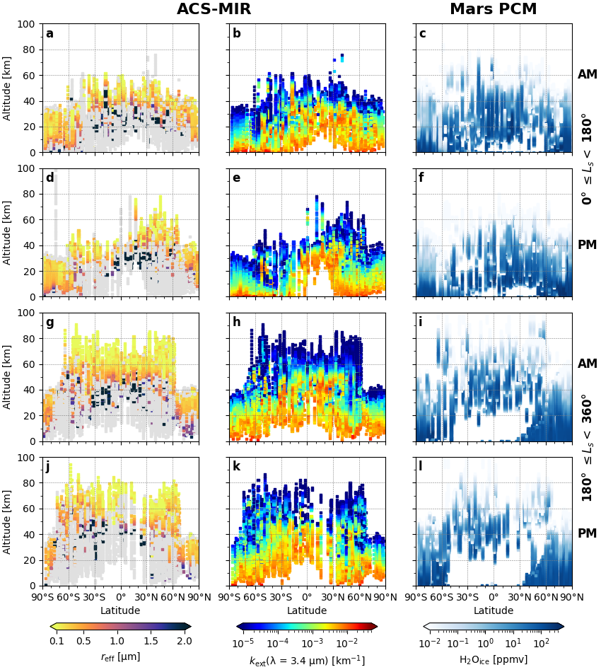
Aurélien Stcherbinine, Guillaume Petzold, Franck Montmessin, Lucio Baggio, Mathieu Vincendon, Michael Wolff, Oleg Korablev, Anna Fedorova, Alexander Trokhimovskiy, and Gaetan Lacombe

Introduction

Water ice clouds play an important role in the Martian water cycle and climate as they are a major actor in the inter-hemispheric water exchange, and impact the atmospheric structure and temperature by absorbing and scattering the incoming solar radiation [1,2 and references contained within]. Plus, we showed in [3] that the vertical structure of the clouds has a non-negligible impact on cloud optical depth retrievals performed from nadir measurements; and in [4] that the version 5 of the Planetary Climate Model (PCM) [5] tends to slightly underestimate the altitude of the water ice clouds. Thus, there is a specific need for a climatology of the vertical structure of the clouds to improve both the atmospheric models, and the nadir clouds surveys that are the main way to perform spatial and temporal surveys of water ice clouds on Mars [e.g., 6,7,8].

Data & Methods

The Atmospheric Chemistry Suite (ACS) Mid-InfraRed (MIR) channel is a high-resolution spectrometer dedicated to Solar Occultation geometry onboard the ExoMars Trace Gas Orbiter (TGO) ESA-Roscosmos spacecraft [10,11]. This observing geometry provides detailed vertical profiles of the atmospheric transmission. In this study, we use ACS-MIR observations acquired in the so-called position 12 of the secondary grating, which covers the 3.1–3.4 µm spectral range to retrieve the properties of the Martian water ice clouds from their 3 µm absorption band using the method described in [12,4].

In 2025 [9], we processed an extended dataset of ~1500 observations, and we reported on the seasonal and latitudinal variations of the Martian water ice clouds from Martian year (MY) 34 (Ls=163°) to MY 38 (Ls=72°). This dataset has now been enlarged to ~2000 observations running until the end of MY 38. The amount of data that we currently have now allows us to combine the MY to reveal the diurnal variation of the cloud’s vertical profiles between the morning and the evening terminator. Plus, we ran the version 6 of the Mars PCM up to MY 37 on the locations of our ACS-MIR observations to compare our vertical profiles with the new version of the model for several MY.

Local time monitoring

The first two columns of Figure 1 show respectively the vertical profiles of the water ice clouds reff obtained between MY 35 and MY 37, and the extinction profiles at 3.4 µm obtained with ACS-MIR during the morning (rows 1 & 3) and the afternoon (rows 2 & 4). We can see that during the first half of the year (aphelion season) the altitude of the clouds is similar between the Northern and Southern hemisphere in the midlatitudes, but in the afternoon the altitude of the clouds increases between 30°N and 60°N, while it decreases in the Southern hemisphere. Another noticeable aspect is that the extinctions are sparser during the morning hours compared to the evening around aphelion. In particular, we can see in panels d & e the presence of a 15-km thick evening layer with high extinction (kext ~ 10-2 km-1) and large water ice crystals (reff > 2 µm). This layer is located between 10°S and 40°N with an altitude ranging between 20 km and 35 km, which corresponds to the aphelion cloud belt (ACB). Then, in panel b, we can see that this layer spread within a wider range of altitude (10-40 km) in the morning.

Comparison with the Mars PCM version 6

The third column of Figure 1 shows the vertical profiles of the amount of water ice as a function of the latitude for the coordinates of the ACS-MIR profiles predicted by the Mars PCM version 6. We observe that when/where the version 5 predicted clouds at altitudes typically 10 km below where they are observed by ACS-MIR in the second half of MY 35 [4], the new version 6 now provides a much better overall agreement with the observations. It may even predict clouds a slightly higher altitude in some cases.

The new version of the model is even able to reproduce the two layers observed in the extinction for Ls > 180° between 30°N and 60°N (panels h, i, k & l). One interesting point is that the PCM predict the presence of clouds in both layers, while our algorithm only flag water ice in the upper one (panels g & j), even though their presence is clearly seen in the extinction. This can suggest that this lower layer is either composed by crystals larger than 3-4 µm which cannot been distinguish from dust in the wavelengths that we are using [12], or mixed with dust.

Figure 1 – Vertical profiles of water ice clouds in the Martian atmosphere (1st column) and atmospheric extinction profiles (2nd column) as observed by ACS-MIR from MY 35 to MY 37, and corresponding water ice vertical profiles from the Mars PCM version 6 (3rd column) as a function of latitude. The profiles are filtered by Ls and local time for each row.

Acknowledgments

ExoMars is a space mission of ESA and Roscosmos. The ACS experiment is led by IKI Space Research Institute in Moscow. The project acknowledges funding by Roscosmos and CNES. Science operations of ACS are funded by Roscosmos and ESA. ACS-MIR level 2B data are available on the LATMOS servers, as described at https://acs.projet.latmos.ipsl.fr/en/data.

References

[1] Clancy et al. (2017) The Atmosphere and Climate of Mars, 76–105. [2] Montmessin et al. (2017) The Atmosphere and Climate of Mars, 338–373. [3] Stcherbinine et al. (2025) Icarus, 425, 116335. [4] Stcherbinine et al. (2022) JGR: Planets, 127, e2022JE007502. [5] Forget et al. (2022) 7th MAMO workshop. [6] Wolff et al. (2022) GRL, 49, e2022GL100477. [7] Smith et al. (2022) GRL, 49, e2022GL099636. [8] Atwood et al. (2024) Icarus, 418, 116148. [9] Stcherbinine et al. (2025) EPSC-DPS 2025, abstract 1495. [10] Korablev et al. (2018) SSR, 214(1), 7. [11] Trokhimovskiy et al. (2015) SPIE, 960808. [12] Stcherbinine et al. (2020) JGR: Planets, 125, e2019JE006300

How to cite: Stcherbinine, A., Petzold, G., Montmessin, F., Baggio, L., Vincendon, M., Wolff, M., Korablev, O., Fedorova, A., Trokhimovskiy, A., and Lacombe, G.: Local time variability of water ice clouds vertical profiles with TGO/ACS-MIR and comparison with the version 6 of the Mars PCM., Europlanet Science Congress 2026, The Hague, The Netherlands, 7–11 Sep 2026, EPSC2026-967, https://doi.org/10.5194/epsc2026-967, 2026.