TP4
Session assets
Orals: Thu, 22 Sep, 12:00–17:00 | Room Manuel de Falla
The NASA InSight Lander on Mars includes the Heat Flow and Physical Properties Package HP3 (see Spohn et al. (2018) for a description of the package) to measure the surface heat flow of the planet. The package uses temperature sensors that would have been brought to the target depth of 3–5 m by a small penetrator, nicknamed the mole. The mole requiring friction on its hull to balance remaining recoil from its hammer mechanism did not penetrate to the targeted depth. Instead, it reached a depth of 40 cm, bringing the mole body 1–2 cm below the surface. A discussion of the lessons learned from the penetration failure and suggestions for an improved mole have been given by Spohn et al. (2022). The root cause of the failure - as was determined through an extensive almost two years long campaign - was a lack of friction in an unexpectedly thick cohesive duricrust. (compare Figure 1)
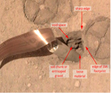
Figure 1. The HP3 mole before complete burial and the properties of the hole that the mole had punched in the duricrust
During the campaign the mole penetrated further aided by friction applied using the scoop at the end of the robotic Instrument Deployment Arm and direct support by the latter. The mole reversed its downward motion twice during attempts to provide friction through pressure on the regolith instead of directly with the scoop to the hull. The penetration record of the mole and its thermal sensors were used to measure thermal and mechanical soil parameters such as the penetration resistance of the duricrust. These parameter values are summarized in Table 1 below. The combined data suggest a model of the regolith that has an about 20 cm thick duricrust underneath a 1 cm thick sand layer and above another 10 cm of sand. Underneath the latter, a layer more resistant to penetration and possibly consisting of debris from a small impact crater was found. The thermal conductivity increases from 14 mW/m K in the 1 cm sand layer to 34 mW/m K in the duricrust and the sand layer underneath the duricrust to 64 mW/m K in the gravel layer below. Applying cone penetration theory, the resistance of the duricrust was used to estimate a cohesion of the latter of 4 - 25 kPa depending on the friction angle of the crust. Pushing the scoop with its blade into the surface and chopping of a piece of crust provided another estimate of the cohesion of 5.8 kPa.
The hammerings of the mole were recorded by the seismometer SEIS and the signals could be used to derive a P-wave velocity and an S-wave as listed (see also Brinkman et al., 2022) representative of the topmost tens of cm of the regolith. Together with a density provided by a thermal conductivity and diffusivity measurement using the mole thermal sensors of about 1211 (Grott et al., 2021), the elastic moduli could be calculated from the seismic velocities.
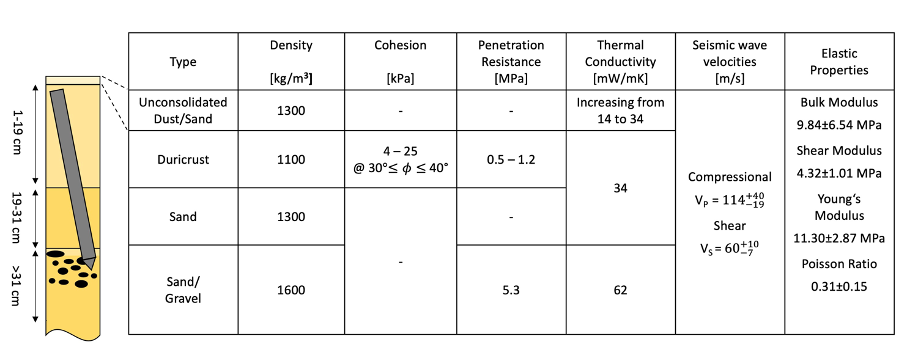
Table 1. Model of the InSight landing site regolith
After burial, the mole was used to measure the thermal conductivity of the regolith as a function of the solar longitude (the seasons on Mars). The variations of the thermal conductivity are consequences of the variations in atmosphere pressure with the seasons and the contribution of atmosphere gas in the porous regolith contributing to the thermal conductivity.
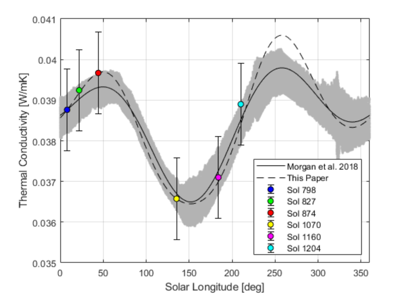
Figure 2 Thermal conductivity in the regolith top 40 cm as measured by sensors on the HP3 mole as a function of the solar longitude (seasons on Mars).
Brinkmann et al. (2022), submitted to J. Geophys. Res. Planets
Grott et al. (2021), Planet and Space Sci, DOI: 10.1029/2019EA000670
Spohn et al. (2018), Space Sci Rev, DOI:10.1007/s11214-018-0531-4
Spohn et al. (2022), Advances in Space Research, DOI: 10.1016/j.asr.2022.02.009
How to cite: Spohn, T., Grott, M., Müller, N., and Hudson, T. and the HP-cubed team: Using the HP3 mole on InSight to probe the thermal and mechanical properties of the Martian regolith, Europlanet Science Congress 2022, Granada, Spain, 18–23 Sep 2022, EPSC2022-408, https://doi.org/10.5194/epsc2022-408, 2022.
Analyses of the InSight seismic data indicate that there are three major seismic discontinuities beneath the lander where the seismic velocity abruptly increases. In addition to the crust-mantle interface at a depth of about 39 km, two major intracrustal discontinuities are observed at depths near 8 and 20 km (Lognonné et al. 2020, Knapmeyer-Endrun et al. 2021, Kim et al. 2021, Duran et al. 2022). There are many possible explanations for the existence of large-scale layering within the crust, and most of these involve a change in either chemical composition or porosity (see Figure 1). Here, we will assess these hypotheses using improved models of the crust that have been made possible by the InSight mission.
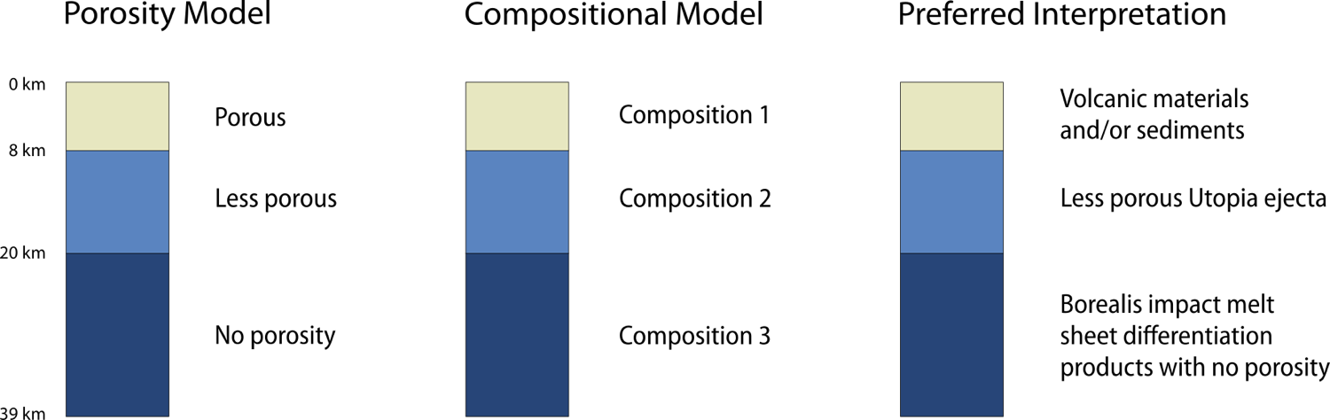
Figure 1. Interpretations of crustal layering beneath the InSight landing site. In the first two schematics, the crustal layering is a result either of stepwise changes in porosity (left) or composition (center). Our preferred interpretation combines elements of both of these end-member models. The depth of each seismic interface below the surface is denoted on the left schematic.
As summarized in Wieczorek et al. (2022), there are a large number of hypotheses for the origin of the three-layered nature of the Martian crust. One or more layers could be composed of volcanic or sedimentary deposits. One of the discontinuities could represent the removal of pore space either by viscous deformation of the host rock or by the precipitation of cements in an ancient aquifer. One layer could represent thick impact basin ejecta deposits, whereas another could represent thick sequences of magmatic intrusions. One of the discontinuities could represent a change in crystallinity, such as is observed in the oceanic crust of Earth. Lastly, one or more discontinuities could be generated by the fractional crystallization of a giant impact melt pool associated with the Borealis impact. Importantly, each of these hypotheses has different implications for the expected thickness of the crustal layer, its composition, and its associated seismic velocity.
Based on the currently available information, we have constructed a plausible model for the observed crustal layering beneath the landing site. As shown in Figure 1, we interpret the uppermost layer as being a result of thick sequences of volcanic materials that were deposited in the early Hesperian, Noachian, and pre-Noachian periods. To account for the low seismic velocities of this layer, these materials would need to be heavily fractured, perhaps being similar in nature to the pyroclastic deposits that make up the nearby Medusae Fossae formation. Given the long duration over which these materials were emplaced, intercalated sedimentary deposits could be common and these materials might also have undergone substantial aqueous alteration at a later date. Ancient impact ejecta deposits from the Utopia basin are likely to be found below the layer of volcanic and sedimentary deposits, potentially in the middle layer between 8 and 20 km depth. The increase in velocity at 20 km depth is likely to be a consequence of the complete viscous closure of all remaining pore space at about 4 Ga when the crustal temperatures were elevated. The deepest layer, from depths of 20 to 39 km, likely corresponds to the initial crust that formed during the differentiation of the Borealis impact melt sheet.
The expected stratigraphy of the southern highlands is less certain. Nevertheless, we speculate that a 20 km seismic discontinuity would be found there as well that represents the transitions from porous to non-porous materials. Another major discontinuity that is likely to be present in the southern highlands would be the base of thick ejecta deposits derived from the ancient Borealis impact event.
It is important to recognize that the InSight landing site is located in the northern lowlands of Mars, and that the layering that is observed beneath the lander might only be indicative of local geologic structure. Future observations of surface waves, as well as analyses of crustal structure at the bounce point of PP waves, will allow us to assess how the thickness of the crustal layers varies across the planet.
References:
Durán, C. et al. (2022). Seismology on Mars: An analysis of direct, reflected, and converted seismic body waves with implications for interior structure. Phys. Earth Planet. Inter., 325, 106851, doi:10.1016/j.pepi.2022.106851
Kim, D. et al. (2021). Improving constraints on planetary interiors with PPs receiver functions. J. Geophys. Res. Planets, 126, e2021JE006983, doi:172810.1029/2021JE006983
Knapmeyer-Endrun, B. et al (2021). Thickness and structure of the martian crust from InSight seismic data. Science, 373, 438-443, doi:10.1126/science.abf8966
Lognonné, P., et al. (2020). Constraints on the shallow elastic and anelastic structure of Mars from InSight seismic data. Nature Geosci., 13, 213-220, doi:175910.1038/s41561-020-0536-y
Wieczorek, M. et al. (2022). InSight constraints on the global character of the Martian crust, J. Geophys. Res., doi:10.1029/2022JE007298
How to cite: Wieczorek, M. A. and the InSight Crust Working Group: Origins of crustal layering beneath the InSight landing site (and elsewhere), Europlanet Science Congress 2022, Granada, Spain, 18–23 Sep 2022, EPSC2022-400, https://doi.org/10.5194/epsc2022-400, 2022.
InSight landed on Mars in November 20181 and carries the InSight FluxGate Magnetometer, IFG2 which has provided the first surface magnetic field measurements on Mars1,3. Previous magnetic field measurements taken at orbital altitudes have provided global coverage, with limited spatial resolution. Laboratory analyses of meteorites provide information on magnetic properties of martian rocks, but without detailed local context for their provenances4. Advances from the IFG are thus unique and complementary science, specifically characterizing the crustal ambient static and external time-varying fields at a single location on Mars. External fields provide information on the planet’s interaction with the interplanetary magnetic field and the ionosphere. Crustal magnetic fields carry information about the ancient dynamo and crustal conditions at the time at which magnetization was acquired, and on how the crust has been modified by subsequent exogenic and endogenic processes4. IFG data for sols 14-736 were collected almost continuously, with some data gaps from electronics anomalies. After sol 736, the magnetometer was operational for shorter periods due to power constraints (Fig. 1) 5. A range of studies have been enabled by IFG data, supported by results from other instruments such as the seismometer, and we summarize those.
Strong crustal fields provide evidence for an ancient dynamo. The IFG measured a surface magnetic field strength of ~2000 nT, ~10x stronger than predicted from satellite data3,6 and consistent with an ancient Earth-like dynamo3. The strong surface field indicates that magnetization at wavelengths shorter than those resolvable from current satellite data (~150 km) contribute substantially to the overall magnetic field. Characterization of the crust through seismic measurements7 and geologic inferences3 of subsurface layering allow assessment of magnetization of the crust (Fig. 2). Depending on the depth at which the magnetization is carried, specifically whether it is in the seismically-determined deep layer of Noachian origin or also in the shallow Hesperian-aged crust, the minimum magnetization required to explain the surface field is ~2 A/m or ~0.4 A/m. Seismic characterization of crustal structure8 indicates a deep subsurface layer (> 20 km, Fig. 2) of no porosity, while the upper crust (<20 km, Fig. 2) is less porous8. Magnetization of these layers require an early active dynamo (>~4 Ga). Fractured, less porous material could have provided pathways for hydrothermal circulation and chemical remanent magnetization4,8,10. Magnetization of the most surficial layer of Hesperian age would be consistent with a long-lasting (up to ~3.7 Ga) dynamo9.
IFG data also reveal time-varying fields at the planetary surface that include contributions with different periods and origins. External fields have been observed and characterized from orbit11–13. However, the degree to which external fields penetrate to and interact with the surface could not be studied prior to the InSight landing. Static and long-duration observations from a surface magnetometer are advantageous because, unlike satellite measurements, temporal variability in the field is not mixed with spatial variability. Here, we summarize different external magnetic field phenomena, transient and periodic that have been observed in IFG data (Fig. 3). Periodic variations include short period waves (100s-1000s3,14), diurnal variations15, the ~26 sol Carrington period associated with solar rotation16, and seasonal15,17 fluctuations. Transient events are observed in response to space weather18 and dust movement19,20.
The inclusion of the magnetometer on InSight has provided unique and substantial scientific contributions to the overall mission results, as well as a starting point for future planetary surface magnetic field investigations. To overcome limitations of current data sets, we look forward to Mars sample return, as well as possible near-surface investigations. Including magnetometers on future missions at a variety of surface locations for long duration observations will be of great value in understanding a range of external field phenomena, including the influence of crustal magnetic fields on ionospheric currents and the effects of space weather during different phases of a solar cycle. We further advocate for regional investigations for example via a helicopter20 that can provide local magnetic field measurements at a spatial scale commensurate with detailed geological knowledge, to further constrain evolution of Mars’ ancient dynamo and explore the magnetic properties of the crust.
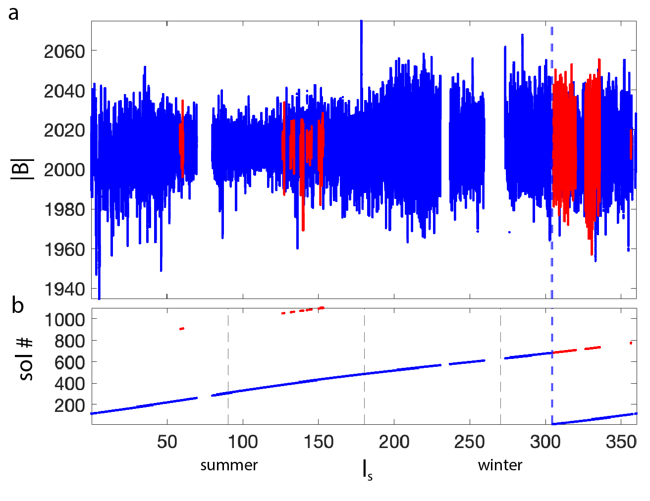
Figure 1: a) Martian years 1 (blue) and 2 (red) of the magnetic field amplitude, B, versus solar longitude (ls). All data up to sol 1106 of InSight operations are included (PDS release 13). The blue vertical dashed line marks the beginning of the mission. (b) Corresponding sol numbers.
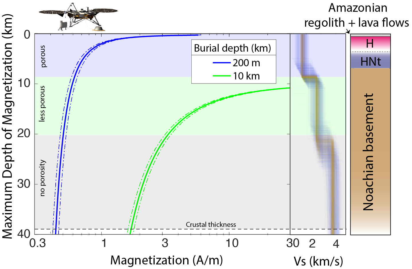
Figure 2: The minimum magnetization required by B=2013 nT (within its 99% confidence intervals)21 for the crust below InSight8. Burial depth describes the depth extent of the unmagnetized layers above the top of the magnetized layer. A burial depth of 200 m (blue), corresponds to burial beneath the young (H: Hesperian, HNt: Hesperian-Noachian transition) near-surface lava flow3 and magnetizations are at least ~0.4 A/m if the entire underlying crust is magnetized. A burial depth of 10 km (blue) requires magnetizations >1 A/m, hosted by Noachian units. The velocity profiles show the seismically-determined interface depths7.
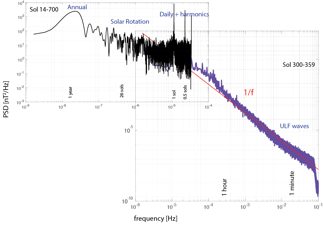
Figure 3: A composite power spectral density (PSD) plot for the surface magnetic field strength at the InSight landing site. Estimates for longer periods are derived using a Lomb-Scargle algorithm (black), shorter periods (purple) show a Welch spectrum.
[1] Banerdt, W. et al. Nat. Geosci. (2020).[2] Banfield, D. et al. SSR (2019). [3] Johnson, C. L. et al. Nat. Geosci.(2020). [4]Mitteholz, A. & Johnson, C. L. Frontiers (2022). [5] Joy, S. et. al. (2019). [6] Smrekar, S. et al. SSR (2018). [7] Knapmeyer-Endrun, B. et al. Science (2021). [8] Wieczorek, M. et al. JGR (2022). [9] Mittelholz, A. et al. Sci. Adv. (2020). [10] Gyalay, S. et al. GRL (2020). [11] Mittelholz, A. et al. JGR (2017). [12] Ramstad, R. et al. Nat. Astron. (2020). [13] Brain, D. et al. JGR (2003). [14] Chi, P. et al. LPSC (2019). [15] Mittelholz, A. et al. JGR (2020). [16] Luo, H. et al. JGR (2022). [17] Mittelholz, A. et al. LPSC (2021). [18] Mittelholz, A. et al. GRL (2021). [19] Thorne, S. et al. PSS (2022). [20] Bapst, J. et al. AAS (2021). [21] Parker, R. JGR (2003).
How to cite: Mittelholz, A., Johnson, C. L., Fillingim, M. O., Joy, S., Langlais, B., Thorne, S. N., Wieczorek, M., Smrekar, S., and Banerdt, W. B.: The surface magnetic field environment from InSight, Europlanet Science Congress 2022, Granada, Spain, 18–23 Sep 2022, EPSC2022-988, https://doi.org/10.5194/epsc2022-988, 2022.
The Martian dichotomy is the most conspicuous feature of the surface of the planet. The difference in elevation between the Northern and Southern hemispheres of Mars likely originates from a difference in crustal thickness. Inversion of topography and gravity data constrained by seismic data from the InSight NASA mission suggests that the southern crust is on average thicker by 18 to 28 km than the northern one if one assumes a uniform crustal density of 2900 kg m-3 (Knapmeyer-Endrun et al., 2021 - Wieczorek et al, 2022).
Several explanations have been proposed for the origin of this crustal dichotomy, involving external processes, such as a large impact (Marinova et al., 2008), or internal ones, such as a degree-one mantle convection (Yoshida and Kageyama, 2006). Here we show that a positive feedback mechanism between crustal growth and partial melting in the mantle could have created this dichotomy. Indeed, because the crust is enriched in heat-producing elements (HPE), the lithosphere of a one-plate planet is thinner where the crust is thicker, inducing a lower pressure at the base of the lithosphere. Because of the pressure-dependence of the mantle solidus, partial melting is more important below a thinner lithosphere, causing a larger rate of melt extraction and crustal growth where the crust is thicker. Larger wavelength perturbations in crustal thickness and extraction, and thus hemispherical perturbations, grow faster because thermal diffusion dampens smaller wavelengths faster.
To model this effect, we use a parametric bi-hemispherical thermal evolution model where a well-mixed convective mantle is topped by two types of lithospheres (North and South) characterized by two potentially different thermal structures (Thiriet et al. 2018). The enrichment in HPE of the crust evolves during crust extraction as the enrichment of the newly formed crustal material depends on mantle melt fraction below the lithosphere, mantle enrichment and partition coefficient. In order to study the growth of a hemispherical perturbation, we impose a small initial difference in lithosphere or crust thickness in between the North and South. We then follow the thermal evolution, mantle melting, crustal growth and crustal enrichment in HPE in both hemispheres over 4.5 Gyr (Fig.1). Our model mainly depends on the mantle reference viscosity, that controls the cooling rate of the convective mantle, on and mantle permeability, that controls crustal extraction from the mantle.
Our results show that this positive feedback mechanism can indeed create a significant crustal dichotomy. The range of North-South crustal thickness differences that we obtain by varying the different model parameters largely encompasses that predicted by inversion of topography and gravity data, assuming different crustal densities. In particular, two types of thermal history allow to reproduce the crustal thickness difference predicted by InSight. The first one is obtained for a rather low viscosity and high mantle permeability; it shows a rapid and early extraction of the crust (Fig1. Solid line) and results in a cold potential temperature at the present-day. The second one is for a higher viscosity and lower mantle permeability; it leads to a late and prolonged extraction of the crust (Fig1. dashed line) and results in a warmer mantle potential temperature and a thicker lid at the present-day. In both cases, the crust is extracted during the first Gyr. The enrichment in HPE of the crust predicted by our model is in agreement with GRS data.

Figure 1 : Evolution of the (a) lid thickness (b) Crust thickness, (c) average melt fraction in the partially melted zone below the lid. (d) Crustal HPE enrichment relatively to the Bulk Silicate Mars as a function of time for the Northern (blue lines) and Southern (orange lines) hemispheres for 2 different simulations that allow to reproduce the difference in crustal thickness deduced from the InSight mission. One evolution (shown in dashed lines) is for a rather high permeability k0 = 9.1.10−10 m2 and low reference viscosity η0 = 4.5x10²⁰ Pa.s, while the second evolution (shown in solid lines) has a lower permeability k0 = 3.72.10−11 m2 and a higher viscosity η0 = 2.02x10²¹ Pa.s.
Acknowledgment :
This project has received funding from the European Research Council (ERC) under the European Union’s Horizon 2020 research and innovation programme (grant agreement No 101001689) and from the ANR (grant MAGIS, ANR-19-CE31-0008-08).
Bibliography :
Knapmeyer-Endrun, B., Panning, M. P., Bissig, F., Joshi, R., Khan, A., Kim, D., Leki ́c, V.,
Tauzin, B., Tharimena, S., Plasman, M., et al. (2021). Thickness and structure of the martian crust
from insight seismic data. Science, 373(6553):438–443.
Wieczorek, M. A., Broquet, A., McLennan, S. M., Rivoldini, A., Golombek, M.,
Antonangeli, D., Beghein, C., Giardini, D., Gudkova, T., Gyalay, S., et al. Insight constraints
on the global character of the martian crust. Journal of Geophysical Research: Planets, page
e2022JE007298.
Marinova, M. M., Aharonson, O., and Asphaug, E. (2008). Mega-impact formation of the mars
hemispheric dichotomy. Nature, 453(7199):1216–1219.
Yoshida, M. and Kageyama, A. (2006). Low-degree mantle convection with strongly temperature-
and depth-dependent viscosity in a three-dimensional spherical shell. Journal of Geophysical Re-
search: Solid Earth, 111(B3).
Thiriet, M., Michaut, C., Breuer, D., and Plesa, A.-C. (2018). Hemispheric dichotomy in litho-
sphere thickness on mars caused by differences in crustal structure and composition. Journal of
Geophysical Research: Planets, 123(4):823–848.
How to cite: Bonnet Gibet, V., Michaut, C., and Wieczorek, M.: A new mechanism for the formation of the Martian dichotomy, Europlanet Science Congress 2022, Granada, Spain, 18–23 Sep 2022, EPSC2022-255, https://doi.org/10.5194/epsc2022-255, 2022.
Seismic measurements of the InSight lander confirm tectonic activity in an extraterrestrial geological system for the first time: the large graben system Cerberus Fossae (Giardini et al., 2020). In-depth analysis of available marsquakes thus allows unprecedented geophysical characterization of an active extensional structure on Mars, using the epicenter locations, depths, magnitudes, focal mechanisms and spectral character from marsquake data. In summary, InSight seismic data show:
- Both major families of marsquakes, characterized by low and high frequency content, LF and HF events respectively, can be located on central and eastern parts of the graben system (Zenhäusern et al., 2022). This is in agreement with the decrease in structural maturity towards the East as inferred from orbital images (Perrin et al., 2022). Specifically, we find that the distance distribution of the larger LF marsquakes peaks near Zunil crater and the Cerberus Mantling Unit, which has been hypothesized to be of volcanic origin (Horvath et al., 2021).
- The two event families correspond to two depth regimes: LF marsquake hypocenters are located at about 15-50 km, based on identification of depth phases (Durán et al., 2022; Stähler et al., 2021), while the HF marsquakes are likely much shallower and at 0-5 km depth (van Driel et al., 2021).
- Estimated magnitudes are between 2.8 and 3.8 (Böse et al., 2021; Clinton et al., 2021), resulting in a total seismic moment release within Cerberus Fossae of 1.4-5.6×10¹⁵ Nm/yr, or at least half of the observed seismic moment release of the entire planet.
- Estimated focal mechanisms of deep marsquakes (Brinkman et al., 2021; Jacob et al., 2022) show primarily extensional normal faulting, compatible with the image-based interpretation as a graben system.
- The deeper LF marsquakes are “slow” compared to terrestrial quakes, i.e. lack high frequency energy in the seismic body waves. This can be explained by low stress drop and a weak, potentially warm source region.
We propose a geological model that integrates these observations: The deep LF quakes are caused by the large-scale extensional stress pattern, while fractures occur in this specific location only due to the presence of a dike from Elysium Mons. The shallow seismicity is caused in a brittle region near the surface, potentially on the subsurface continuation of the graben flanks. This could potentially explain the seasonality of the HF event rate, which peaks at the times of maximum solar illumination of the bottom in the Cerberus Fossae (Knapmeyer et al., 2021).
While a small number of large endogenic marsquakes have been observed in other regions on Mars, specifically Southern Tharsis (Horleston et al., 2022), Cerberus Fossae represents a uniquely active seismic setting. Current day tectonic activity seems to be driven by volcanic processes, and furthermore, we find no trace of seismic activity on compressional thrust faults on Mars, as opposed to the models of seismicity driven by secular cooling and lithospheric contraction.
References:
Böse, M., et al., 2021. Magnitude Scales for Marsquakes Calibrated from InSight Data. Bull. Seismol. Soc. Am. https://doi.org/10.1785/0120210045
Brinkman, N., et al., 2021. First focal mechanisms of marsquakes. J. Geophys. Res. Planets. https://doi.org/10.1029/2020je006546
Clinton, J.F., et al., 2021. The Marsquake catalogue from InSight, sols 0–478. Phys. Earth Planet. Inter. 310. https://doi.org/10.1016/j.pepi.2020.106595
Durán, C., et al., 2022. Seismology on Mars: An analysis of direct, reflected, and converted seismic body waves with implications for interior structure. Phys. Earth Planet. Inter. 325, 106851. https://doi.org/10.1016/j.pepi.2022.106851
Giardini, D., et al., 2020. The seismicity of Mars. Nat. Geosci. 13, 205–212. https://doi.org/10.1038/s41561-020-0539-8
Horleston, A., et al., 2022. The far side of Mars - two distant marsquakes detected by InSight. Seism. Rec. accepted.
Horvath, D.G., et al., 2021. Evidence for geologically recent explosive volcanism in Elysium Planitia, Mars. Icarus 365, 114499. https://doi.org/10.1016/j.icarus.2021.114499
Jacob, A., et al., 2022. Seismic sources of InSight marsquakes and seismotectonic context of Elysium Planitia, Mars. Tectonophysics in revision.
Knapmeyer, M., et al., 2021. Seasonal seismic activity on Mars. Earth Planet. Sci. Lett. 576, 117171. https://doi.org/10.1016/j.epsl.2021.117171
Perrin, C., et al., 2022. Geometry and Segmentation of Cerberus Fossae, Mars: Implications for Marsquake Properties. J. Geophys. Res. Planets 127, e2021JE007118. https://doi.org/10.1029/2021JE007118
Stähler, S.C., et al., 2021. Seismic detection of the martian core. Science 373, 443–448. https://doi.org/10.1126/science.abi7730
van Driel, M., et al., 2021. High-Frequency Seismic Events on Mars Observed by InSight. J. Geophys. Res. Planets 126, e2020JE006670. https://doi.org/10.1029/2020JE006670
Zenhäusern, G., et al., 2022. Low Frequency Marsquakes and Where to Find Them: Back Azimuth Determination Using a Polarization Analysis Approach. ArXiv220412959 Phys.
How to cite: Stähler, S. C., Mittelholz, A., Perrin, C., Kawamura, T., Kim, D., Knapmeyer, M., Zenhäusern, G., Clinton, J., Giardini, D., Logonné, P., and Banerdt, W. B.: Seismicity unveils tectonics in Cerberus Fossae, Mars, Europlanet Science Congress 2022, Granada, Spain, 18–23 Sep 2022, EPSC2022-1126, https://doi.org/10.5194/epsc2022-1126, 2022.
In August 2021, the first seismological determination of the core radius of Mars was published by the InSight team (Stähler et al., 2021). We take this opportunity to take a mental step backwards and assume a historical perspective on the scientific investigation of planetary cores, and how our knowledge about them, especially in terms of their size, evolved.
The first thoughts about the Earth's interior that we would place into the history of science or rather into that of religion originate in the 17th century. Descartes suggested that the Earth is a former star which produced so many sunspots that it became encrusted in them, and that later processing of sunspot-material resulted in the surface we have today. The innermost part of the Earth, however, is still unaltered solar matter.
Isaac Newton, in the posthumously published "System of the World", suggested that the gravity of a single, isolated mountain could be used to determine the density ratio between the surface and the interior of the Earth. Respective experiments were conducted by Bouguer and, later, by Maskelyne and Hutton - the latter concluded from the result, that the presence of a heavy, metallic core could explain the overall mass of the Earth as well as the density contrast resulting from Newton's experiment. A metallic core was also suggested by Wiechert, by the end of the 19th century. When Oldham demonstrated the S wave core shadow in 1906, he did not make any suggestions about the nature of the central region.
In the early 20th century, it was however doubted that any material could withstand the conditions of the deep interior, or that a segregation of metals could take place. One alternative approach was indeed solar matter, another one a metallic high pressure state of silicate rock: The possibility that the core mantle boundary is a phase boundary like the 410 and 660 km discontinuities was long supported by some.
The consequence of the phase boundary model was that neither the Moon nor Mars could have cores, for the simple reasons that they are too small to provide the necessary internal pressures. This claim fit well with the moment of inertia factors as they were observed back then: Until the mid-1960s it was assumed that the MoIF of the Moon exceeds 0.4, and that of Mars is too close to 0.4 to indicate much differentiation.
In both cases, the space age led to a revision: Having spacecraft near or at the respective bodies turned out to be crucial for a sufficiently precise determination of the MoIF.
In the case of Mars, the Mariner IV mission greatly improved the knowledge of radius, mass, and moment of inertia factor of the planet (because of the atmosphere, even the radius was rather uncertain and observational results depended on the optical wavelength used in photography). After Mariner IV, an iron core suddenly became feasible, if not necessary, again. Mariner VI and VII showed that Mars is neither a small Earth nor a big Moon, but something different - and the global photographic map resulting from the Mariner IX mission showed all the now familiar surface structures for the first time. With Mariner IX it also became possible to map the surface gravity, and the gravity anomaly of Tharsis was discovered - which is so enormous that it biases the J2 gravity coefficient, and invalidates the previously used hypothesis of hydrostatic equilibrium. Several methods to compensate for this were suggested in the following. A replacement for the hydrostatic assumption became available with precession measurements using Viking radio signals, later augmented by Pathfinder and other missions. It became finally possible to determine the MoIF, which turned out to be significantly below that of the homogeneous sphere. The most significant progress in terms of the estimation of the core radius was however Mariner IX: After this mission, core radii below 1000 km were no longer discussed.
The Viking missions produced important clues for the identification of the SNC meteorites as of martian origin, and thus for improved models of the chemical composition of Mars. This provided better contraints for the densities of core and mantle. A comparison of the core radii discussed in the literature after Viking however shows that none of these models could constrain the core radius with a sufficient precision. Different models were developed, but in the long run, the range of uncertainty of the core radius proved rather stable for more than 40 years.
The results obtained by InSight still build upon the knowledge of geodetic and gravity measurements as well as on geochemistry, but they add seismic data as constraints that are more sensitive to the sought-after structural parameters than to density.
References
Listing all references relevant for the above text would require much more space than is available here. The discussion of the abstract is a condensate from Knapmeyer & Walterová (2022), where all the references can be found.
Knapmeyer, M., Walterová, M. (2022), Planetary Core Radii: From Plato towards PLATO, under review at Advances in Geophysics.
Stähler et al., (2021). Seismic detection of the martian core, Science, vol. 373, 443-448, DOI: 10.1126/science.abi7730
How to cite: Knapmeyer, M. and Walterová, M.: The core radius of Mars: a historical perspective, Europlanet Science Congress 2022, Granada, Spain, 18–23 Sep 2022, EPSC2022-803, https://doi.org/10.5194/epsc2022-803, 2022.
Introduction
Wrinkle ridges are significant landforms on planetary bodies, and most of them occur in flood basalt units of large igneous provinces, [1]-[2]. On Mars, the circum-Tharsis wrinkle ridge system developed under compressional stresses associated with the response of the lithosphere due to the Tharsis volcanic load [1]. The morphology of ridges shows large variations and may reflect subsurface fault patterns [3]–[5]. Numerous studies on their physical dimensions [6]–[10], their accommodated horizontal strain (e.g., [11]–[12]), as well as a variety of conceptual formation models (e.g., [13]–[17]) have been performed to better understand the morphologies and geodynamic significance of wrinkle ridges. A variety of tectonic models including buckling, thrust/reverse faulting, fault-bend folding, and fault propagation folding have been proposed to explain the formation of wrinkle ridges(e.g., [9]–[19]).
Even though there are many studies on wrinkle ridges, it is still uncertain what the subsurface of these structures looks like. To get insights into the subsurface we selected sites, where deep morphological incisions provide such exposures. Hence, we used steep escarpments formed by impact craters, collapse pits, and valleys. A prerequisite for this study is the availability of high-resolution remote sensing data and digital elevation models to investigate the fault patterns that exist in the subsurface of wrinkle ridges.
Methodology
We used High-Resolution Imaging Science Experiment (HiRISE) (~0.25 m/px) [20], and Context Camera (CTX) (~6–7 m/px) [21] satellite imageries to generate high-resolution digital elevation models (DEMs) by using the Ames Stereo Pipeline [22] in combination with the Integrated System for Imagers and Spectrometers (ISIS) software [23]. CTX and HiRISE DEMs with the digital raster graphic (DRG) files were used to analyze and measure topographic offsets. We have selected twelve different study areas (with multiple outcrops from A to D) that all belong to the system of circum-Tharsis wrinkle ridges. Our area of interest includes regions at Solis Planum, at the borders of Nilus Dorsa, at the Coprates Chasma, at the south of Lunae Planum, and the Thaumasia Planum that shares significantly akin structures with a south of the Mela's Fossae (Fig. 1).

To measure the strike and dip of fault planes we used two methods: (i) we applied the LayerTools [24] add-in for ArcGIS Software and (ii) we constructed manually the strike of faults by connecting points along the fault trace that have of the same elevation. The dip angle is determined perpendicular to the strike direction by recording intersection points of the fault trace with different elevation levels. We mapped all fault intersection lineations (red lines) on wrinkle ridges.
Results
Here, we present only two of twelve case study results. Fig. 2 (study area 1) shows that folding and faulting are intimately linked to each other. The outcrop sections show that the slopes of the wrinkle ridge are formed by the limbs of a vergent anticline. The dip of two subordinate thrust faults with NNW-SSE strike directions could be determined (38° and 46°). In Fig. 3 (study area 2), the western part of the flat crater floor is elevated by ~100 m with respect to the eastern crater floor. Along with this occurs a change in polarity of the fault with a dip direction to the east in the northern crater section and a westward dip in the southern crater section. The wrinkle ridge shows complex fault pattern north and south of the crater, where faults cut obliquely through the wrinkle ridge.
Discussion and Conclusion
Both reverse (>45°) and thrust (<45°) faults are frequent in the subsurface of wrinkle ridges and along with the anticlinal folding document that horizontal compression is the driver for their formation. A multitude of subsidiary and splay faults exist. Symmetric wrinkle ridges contain a conjugate system of thrusts or reverse faults. Asymmetric wrinkle ridges have one dominant reverse/thrust that reaches the surface at the base of the steeper slope. In such cases, additional antithetic faults are subordinate and merge into the main fault. A polarity change of wrinkle ridges can take place along strike and is associated with a change in the amount of displacement that is accommodated along the faults. The fault with the largest amount of slip is situated beneath the ridge crest and steeper slope. Several wrinkle ridges display the main thrust fault whose dip angle abruptly gets shallower at a depth of 500-1000 m beneath the surface. The application of fault-propagation fold models to wrinkle ridges [14]-[19] show conditionally the best match to observations.


References: [1] Scott D. H. and Tanaka K. L. (1986) USGS,1802. [2] Strom R. G. et al. (1975) JGR, 80, 2478–2507. [3] V.L. Sharpton and J. W. Head (1988) LPSC XVIII, Abstract#307.[4] Plescia J. B. and Golombek M. P (1986) Bull. Geol. Soc. Am., 97, 1289–1299. [5] Strom R. G. (1972), Dordrecht: Springer Netherlands, 187–215. [6] Mueller K. and Golombek M. (2004) Annu. Rev. Earth Planet. Sci., 32, 435–464. [7] Watters T. R. and Robinson M. S. (1997) JGR Planets, 102,10889–10903. [8] Golombek M. P. and Phillips R. J (2010) Eds. Cambridge University Press,183–232. [9] Golombek, M. P. et al. (1991) LPS XXI, Abstract#679. [10] Mangold N. et al. (1998) Planet. Space Sci., 46, 345–356. [11] Plescia J. B. (1991) Geophys. Res. Lett., 18, 913–916. [12] Montési L. G. J. and Zuber M. T. (2003) JGR Solid Earth, 108,1–16. [13] Allemand P. and Thomas P. G. (1995) JGR, 100, 3251. [14] Schultz R. A. (2000) JGR Planets, 105, 12035–12052. [15] Watters T. R. (2004), Icarus, 171, 284–294. [16] Karagoz O. et al. (2022) Icarus, 374,114808. [17] Chester, J., and Chester, F., (1990) Struct. Geol. 12, 903–910 [18] Suppe J. and Medwedeff D. A. (1990) Eclogae Geol. Helv., 83, 409–454. [19] Suppe J. and Medwedeff D. A. (1984) GSA 16, Abstract#670. [20] McEwen et al., (2007) JGR, 112, E05S02. [21] Malin et al., (2007) JGR, 112, E05S04. [22] Moratto Z. M. et al. (2010) LPSC XLI, Abstract#2364. [23] Becker, K. J. et al. (2013) LPSC XLIV, Abstract#2829. [24] Kneissl et al., (2010) LPSC XLI, Abstract#1640.
How to cite: Karagoz, O., Kenkmann, T., and Wulf, G.: Clues to the subsurface fault pattern of circum-Tharsis wrinkle ridges, Europlanet Science Congress 2022, Granada, Spain, 18–23 Sep 2022, EPSC2022-59, https://doi.org/10.5194/epsc2022-59, 2022.
Introduction: The edge of the pre-Noachian Borealis impact basin, thought to be the cause of the planetary dichotomy boundary [1-2], crosses the northern Valles Marineris troughs [1-3]. Intense deformation is exposed in the deepest parts of the Ophir and Hebes Chasmata, the northernmost troughs. Structural geology and mineralogical analyses motivate the tentative identification of brittle and brittle-ductile shear zones and hydrothermal activity in the Valles Marineris basement. Implications for the Borealis basin and the proto-Valles Marineris crust are examined.
Structural analysis: Crustal right-lateral shear zones are identified in the pre-Noachian basement of Ophir and Hebes Chasmata (Figure 1). In Ophir Chasma, S-C-C' structures, indicate deformation in the brittle-ductile domain. In Hebes Chasma, megabreccia indicates brittle deformation. From scaling relationships [4-5], the shear zones are inferred to be at least hundreds of kilometers long. They do not extend to the surface nor even up into the interior layered deposits (ILD), and are therefore interpreted to affect the Valles Marineris basement only, which at this depth, is interpreted to be of pre-Noachian age.
Mineralogy: A new method of non-linear spectral unmixing derived from the LinMin algorithm [6] is implemented and applied to three pre-Noachian basement exposures in a CRISM cube in Ophir Chasma. After gas absorption removal, two groups of minerals are robustly detected (Figure 2): primary minerals of mafic rocks (olivine, hypersthene, augite, anorthite, albite), and sulfates, most of them likely of hydrothermal origin (copiapite, jarosite, szomolnokite). Anhydrite (ROI3) is not diagnostic of any particular environment. Kieserite is interpreted as transported by wind from the neighboring ILDs. S-C-C' structures constrain the granulometry of the sheared rock which, under the assumption that all the primary minerals are detected, would be olivine-gabbronorite (ROI1) or troctolite (ROI2-3). Combined structural and mineralogical analyses point to hydrothermal alteration of a mafic intrusive basement, or contamination of this basement by hydrothermal activity in the ILDs.
Relationships with the Borealis basin: The general trend of the shear zones follows the edge of the Borealis as inferred from gravity and topography [4], also of pre-Noachian age, suggesting that they may have initiated as basin ring faults and were reactivated as crustal shears. North of Valles Marineris, the radial component of the remanent magnetic field at the surface [7] shows elongated anomalies that follow the trend of the shear zones and more generally, the expected curved edge of the Borealis basin. The existence of a magnetic field (or dynamo) was coeval with formation of the planetary dichotomy boundary [8]. Two anomalies also correspond to Noachian or pre-Noachian crustal ridges in Ophir Planum, of igneous [9] or tectonic [10] origin. Mapping reveals that the ridges are fractured parallel to the magnetic anomalies, and that their topography guided a hydrologic system (Figure 3). Moreover, these fractures are parallel to a dyke swarm exposed in eastern Candor Chasma [11]. Therefore, the ridges have a volcanotectonic origin within an active hydrologic context.
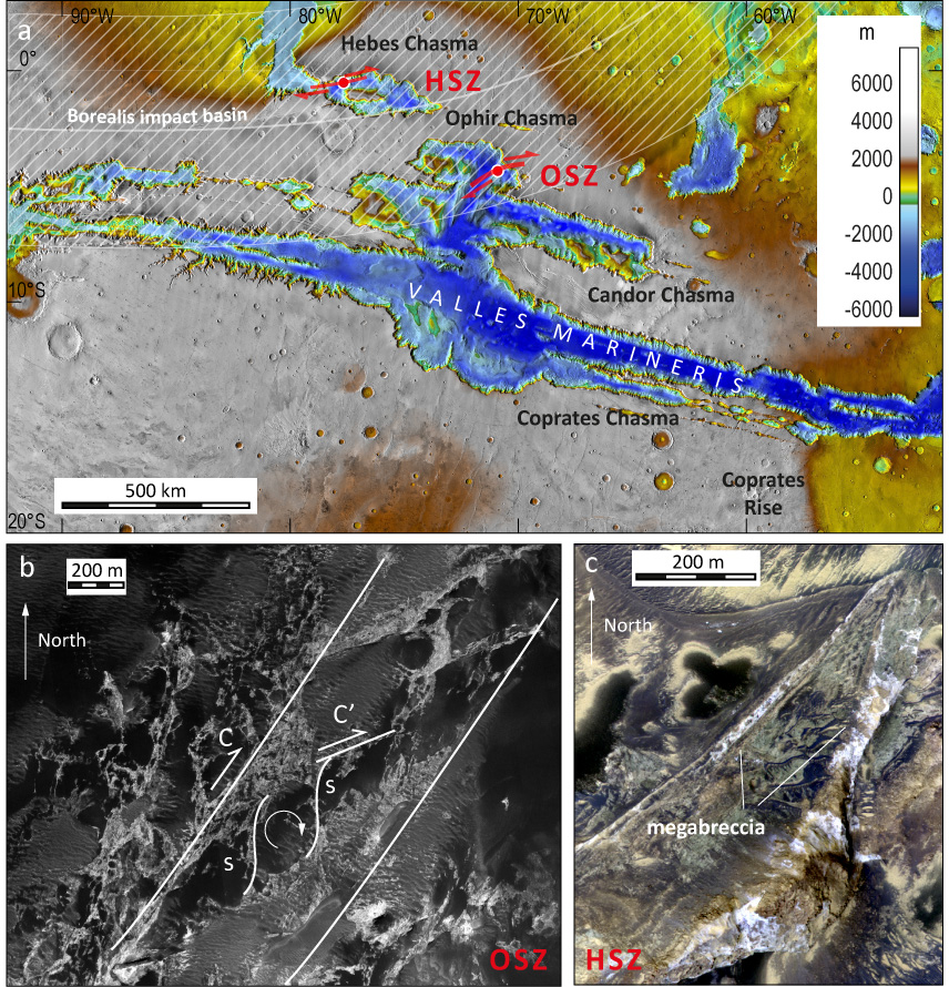
Figure 1. Ophir shear zone (OSZ) and Hebes shear zone (HSZ): (a) location map showing trace of the Borealis impact basin with ±5° uncertainty (dashed area) [5]; (b) zoom on S-C-C' structures in the OSZ, and illustration of shear orientations; (c) zoom on fault megabreccia in the HSZ. HiRISE images ESP_017754_1755 and ESP_040211_1790.
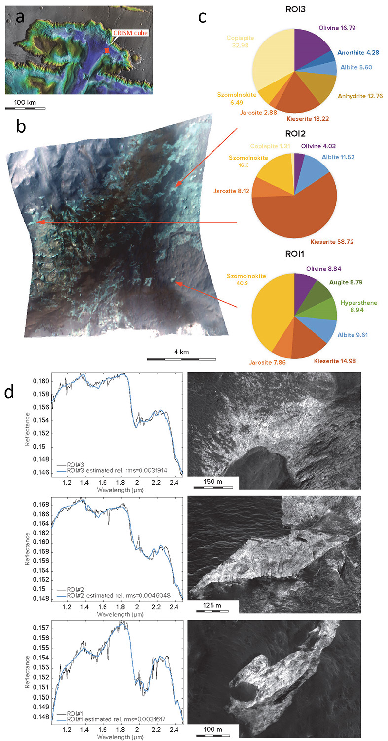
Figure 2. Results of nonlinear spectral unmixing applied to basement exposures in Ophir Chasma: (a) CRISM cube location (frt00018b55_07_if165l_trr3); (b) the cube (bands R: 233, G: 78, B: 13); (c) mineral relative abundances, after aerosol contribution removal; (d) best fit plots and HiRISE images of the basement exposures: ESP_051999_1755, ESP_039525_1755, ESP_039525_1755.
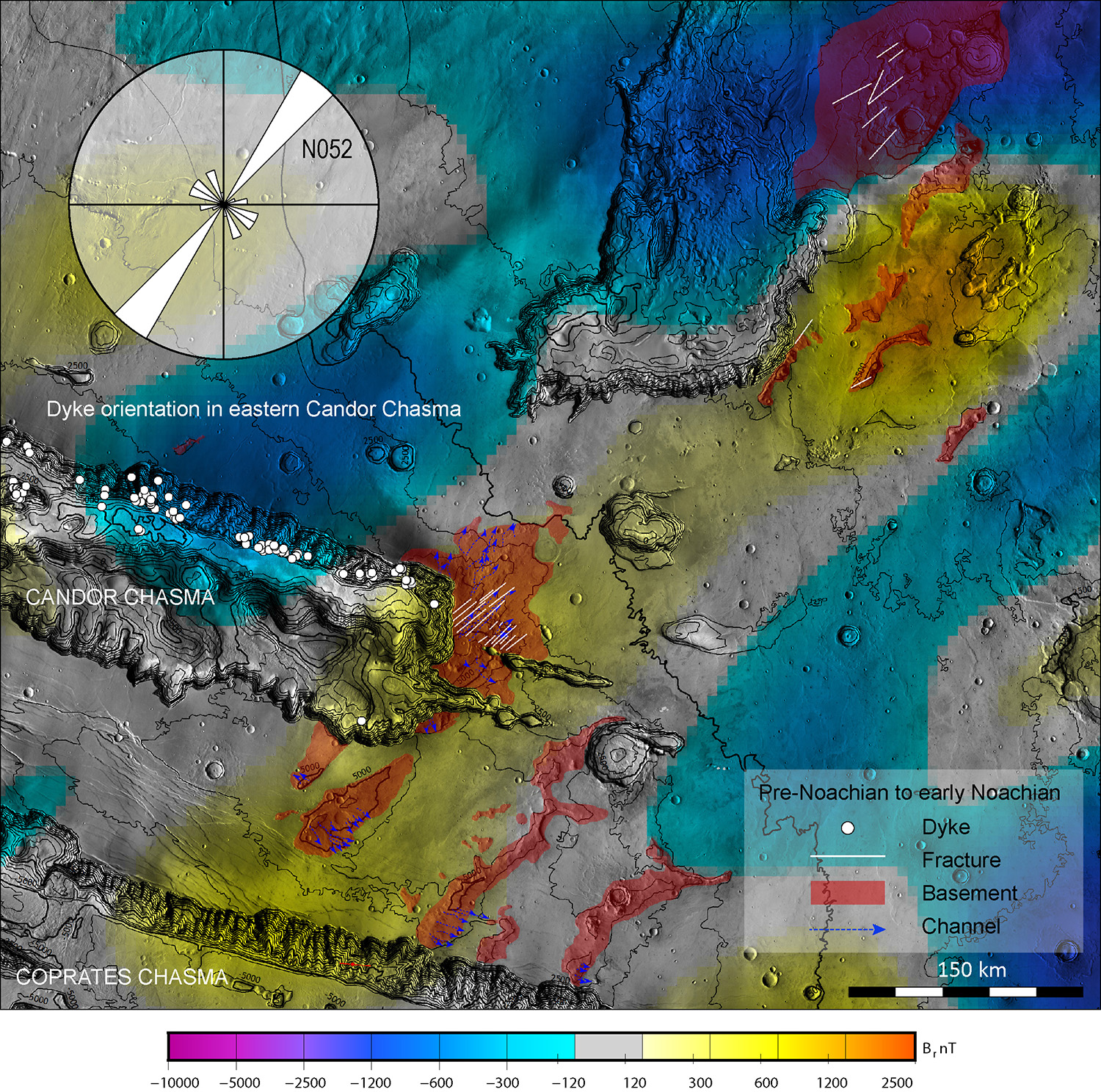
Figure 3. Features related to hydrothermal activity possibly resulting from the Borealis impact and suggested to explain magnetic banding north of Coprates Chasma. Dykes are located thanks to HiRISE images. The rose diagram was established from 26 representative dykes observed on the eastern Candor Chasma wall; the indicated strike refers to the mean resultant dyke orientation. Magnetic anomalies are from [7]. Topographic contours (spacing 500 m) are from HRSC (ESA/DLR/Freie Univ. Berlin).
Circumferential magnetic anomalies are observed at some terrestrial impact craters (e.g.[12]) as well as the Chicxulub impact basin [13] and are due to crystallization of magnetic minerals in an impact-related hydrothermal system [14]. We suggest, therefore, that the magnetic anomalies measured above the Valles Marineris plateau similarly result from hydrothermal activity in response to the Borealis impact, and follow basin ring structures. This hydrothermal activity might be the surface counterpart of deep hydrothermal activity in the basement detected using spectral unmixing [15].
Conclusions: Analysis of northeastern Valles Marineris supports the interpretation of a pre-Noachian Borealis impact basin that would have underlain the later northern troughs of Valles Marineris in the presence of an active dynamo. Large shear zones in the Valles Marineris basement would be reactivated ring faults. Borealis basin formation may have triggered a huge hydrothermal system, identified along these structures and also producing magnetic minerals that generated the observed magnetic anomalies. Primary deposits of base and rare metals likely formed as well. Other evidence of hydrothermal activity at the edge of the Borealis basin would confirm these interpretations.
References: [1] Andrews-Hanna J. et al. (2008) Nature, 453, 1212–1215. [2] Marinova M. M. et al. (2008) Nature, 453, 1216–1219. [3] Andrews-Hanna J. (2012) J. Geophys. Res., 117, E03006. [4] Schultz R. A. and Fossen H. (2002) J. Struct. Geol. 24, 1389–1411. [5] Fossen H. (2010) Structural Geology, Cambridge Univ. Press. [6] Schmidt F. et al. (2014) Icarus, 237, 61–74. [7] Langlais B. et al. (2019) J. Geophys Res., 109, E02008. [8] Mittelholz et al. (2020) Sci. Adv., eaba0513. [9] Tanaka K. L. et al. (2014) USGS Sci. Inv. Map 3292. [10] Viviano-Beck et al. (2017) Icarus, 284, 43–58. [11] Mège D. and Gurgurewicz J. (2017) 48th LPSC, Abstract #1087. [12] Hawke P. J. et al. (2006) Explor. Geophys., 37, 191–196. [13] Abramov O. and Kring D. A. Meteor. Planet. Sci., 42, 93–112. [14] Osinski G. R. et al. (2011) Meteor. Planet. Sci., 36, 731–745. [15] Gurgurewicz J. et al., submitted to Commun. Earth Environ.
How to cite: Mège, D., Gurgurewicz, J., Schmidt, F., Schultz, R. A., Douté, S., and Langlais, B.: Tectonic and hydrothermal activity at the edge of the Borealis impact basin in Valles Marineris, Europlanet Science Congress 2022, Granada, Spain, 18–23 Sep 2022, EPSC2022-116, https://doi.org/10.5194/epsc2022-116, 2022.
Fault population studies are essential to investigate lithospheric strength and stress conditions [1]. Understanding the displacement-length relationship of faults helps us to understand the lithosphere and stress states, and may inform on the stratigraphy of crustal rocks [2]. However, the number of slip events, linkage, and reactivation may affect the Dmax/L ratios [3]. The investigation of current seismicity on Mars is the motivation for a renewed and detailed analysis of the fault systems of Mars. Using Digital Elevation Models (DEM) and corresponding orthoimages derived from High Resolution Stereo Camera (HRSC) data, we obtained information on the displacement distribution on fault traces as well as the maximum displacement. The Dmax/L ratio is calculated as ~0.007, consistent with previous measurements of martian faults (0.006; [4]). Based on these analyses, we discuss the implications of fault segmentation and linkage for further interpretation.
IntroductionDetailed investigation on geometric fault properties can provide insights into the mechanical and temporal evolution of fault systems [5,6], and the past and future potential for seismic energy release [7]. In planetary science, where a lack of seismometers is unfortunately the rule rather than the exception, the analysis of faults with remote sensing data typically provides the only direct observational evidence to constrain the tectonic history of a planet [1]. Since the seismic moment released during the growth of a fault is strongly connected to the fault geometry, the study of fault populations can also help to estimate the current seismicity level [2,8]. Until today, only a few data on the relationships between fault displacement and length have been collected for extraterrestrial bodies [9], partly due to the limited number of reliable topographic datasets.
The InSight mission put a lander in the Elysium region of Mars in 2018. It is equipped with a seismometer [10] that has recorded several marsquakes for which the locations could be determined [11]. As a starting point for our analysis of fault geometries, we selected the Memnonia Fossae fracture system, one of the closest fracture sets to the InSight landing site, which radiates outward from the Tharsis region in a southwesterly direction.
Data and MethodsAll topographic measurements in this study are based on Digital Elevation Models (DEM) based on HRSC data (High Resolution Stereo Camera; [10]). As HRSC is a push-broom scanning instrument with nine CCD line detectors mounted in parallel on a focal plane, its unique feature is the ability to obtain imaging data at high resolution, with along-track triple stereo, four colors and five different phase angles. The spatial scale of HRSC is 10 m/pixel at the nominal periapsis altitude of 250 km, with an image swath of 53 km.
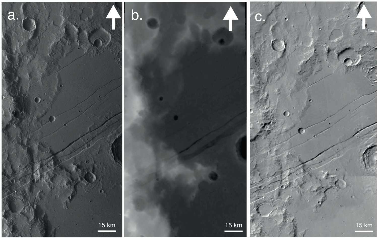
Figure 1: Images show faults from Memnonia Fossae region with three different image system: a. Orthoimage from HRSC, b. DEM derived from HRSC data, c. CTX image.
We use DEM and orthoimages from HRSC [10] to obtain information on the displacement distribution along fault traces. This also enabled determining the maximum displacement. We compare our results to previous measurements of faults on Mars, Earth, and beyond. Based on these analyses, we discuss the implications of fault segmentation and linkage for further interpretation. HRSC data offer high-resolution topography and spatially contiguous coverage, which are required to analyze detailed topographic characteristics of large fault systems. For structural interpretation of key locations (e.g., relay ramps), CTX images (~5-6 m px-1) have been inspected. Fault length was digitized along the fault line, and multiple topographic cross-sections across the fault were drawn with a spacing of ~1 km. Fault throw (a proxy for true displacement) was visually determined in the digitized cross-sections.
Results
At the time of writing, 16 images out of 75 available images/DEM from the Memnonia Fossae region exhibiting normal faults have been investigated. In this preliminary stage, a total number of 83 faults in Memnonia Fossae were studied. We find an average Dmax/L ratio of 0.007, consistent with our previous findings for other regions on Mars, where this ratio had an average value of 0.006 [4].
References
[1] Schultz, R.A. et al. (2010) J. Struct. Geol., 32, 855-875. [2] Golombek, M.P. et al. (1992) Science 258, 979-981. [3] ] Kim, Y., Sanderson, D. J. (2005) Earth Sci. Reviews, 68, 317-334. [4] Hauber, E. et al. (2014) Lunar Planet. Sci. Conf. 45, #1981. [5] Cartwright, J. A., et al., J. Struct. Geol. 17, 1319-1326, 1995. [6] Cowie, P.A. and Scholz, C.H., J. Struct. Geol. 14, 1133-1148, 1992. [7] Wells, D.L. and Coppersmith, K.J. (1994) Bull. Seismol. Soc. Amer., 84, 974-1002. [8] Knapmeyer, M. et al. (2006) J. Geophys. Res., 111, E11006. [9] Schultz, R.A. et al. (2006) J. Struct. Geol., 28, 2182-2193. [10] Lognonné, P., et al., (2019) Space Science Reviews, 215(1), 1-70. [11] Drilleau, M., et al., (2021) EGU General Assembly. Conf. 14998. [12] Gwinner et al., Planetary and Space Science 126 (2016) 93–138.
How to cite: Yazici, I., Hauber, E., and Tirsch, D.: Fault scaling at Memnonia Fossae, Mars: Displacement-length relationship derived from HRSC data, Europlanet Science Congress 2022, Granada, Spain, 18–23 Sep 2022, EPSC2022-1105, https://doi.org/10.5194/epsc2022-1105, 2022.
On Mars, prominent thick-layered sulfate-bearing deposits are observed at a number of late Noachian to late Hesperian locations (~3.5 Ga) [1]. Their apparent absence in older strata has led to the hypothesis that they represent ancient evaporites related to the global aridification [2]. In Gale crater, the Curiosity rover is now exploring the Layered Sulfate-bearing unit (LSu), which is a hundreds of meters thick regional package of yet unknown origin within the Mt Sharp group (Fig. 1). Curiosity investigations can test whether its formation processes are similar to the Burns fm., another major sulfate-bearing strata documented by the Opportunity rover, or distinct such as a form of primary evaporites, syndiagenetic or later stage diagenetic precipitations with different aqueous conditions.
After exploring the mudstone-rich strata of the Murray and Carolyn Shoemaker fm. for about seven years, the Curiosity rover entered the LSu in 2021. Bedrock in the basal section is marked by diverse diagenetic overprints where sedimentary structures are less visible. In some places, laminated mudstones or siltsontes associated with concretions and with mm-scale nodular features may present similarities to evaporitic textures previously observed in the Murray formation [3]. Further up, the rover imaged butte-forming outcrops (Fig. 1) and revealed a ~100-m-thick interval with a transition into large-scale trough cross-bedded structures, the lithology, scale and thickness of which has never been observed before by the rover at such close range [4].
The base of the LSu succession is marked by a sharp increase in density of bedrock nodular textures. The rover analyzed the composition of two bedrock components: (i) a smooth host bedrock, which was drilled several times, revealing the disappearance of clay minerals in X-ray diffraction [5] – the evolved gas analyses also suggest Mg-sulfates and an isotopic change in sulfur compared to the clay-bearing unit below [6]; (ii) a nodular bedrock, which was not drilled due to its uneven surface, but shows diverse sulfate-enriched compositions as measured by ChemCam. Overall, the bulk bedrock (combining smooth and nodular) shows an increase in sulfate content relative to prior strata, nodular textures being a key component of that change (Fig. 2). Unusual lithologies have been observed in the basal LSu, including a regular pattern of polygonal ridges (Fig. 2), clearly crosscut by later stage fractures, pointing to multiple phases of diagenetic alteration. These sulfate-enriched polygonal ridges may represent the first evidence of a paleosol on Mars formed by sustained wet-dry cycles at the surface [7].
The LSu shows multiple signs of marked changes towards drier paleoenvironments in the sedimentary and geochemical record. Within the large-scale cross-bedded strata of most likely eolian origin sulfates in the LSu differs from the Burns fm. homogeneous enrichments as they occur in the form of diverse heterogeneities mostly related to nodular bedrock. Ongoing exploration could help test whether the drying-upward transition reflects internal basin controls on the evolution of ancient Gale lake or external, possibly global, climatic controls.
References: [1] Ehlmann B. L. and Edwards C. S. (2014) Annu. Rev. Earth Planet. Sci. 42, 291–315. [2] Bibring J.-P. et al. (2006) Science 312, 400–404. [3] Schieber et al. (2022) LPSC #1034. [4] Rapin W. et al. (2021) Geology 49, 842–846. [5] Rampe et al. (2022) LPSC #1532. [6] Clark et al. (2022) LPSC #1160. [7] Goehring L. et al. (2010) Soft Matter 6, 3562–3567.
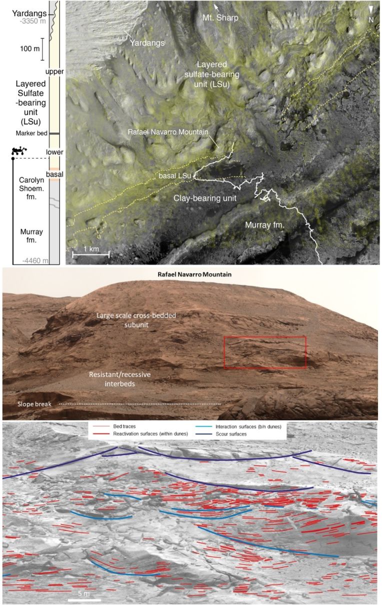
Figure 1: Context of the Layered Sulfate-bearing unit (LSu) exploration by the Curiosity rover. Top to bottom: map with rover traverse and general stratigraphic column; architecture of deposits observed on Rafael Navarro Mountain outcrop; example RMI close-up (red) showing evidence of large-scale cross-bedded sedimentary structures with possible hierarchy of eolian surfaces.
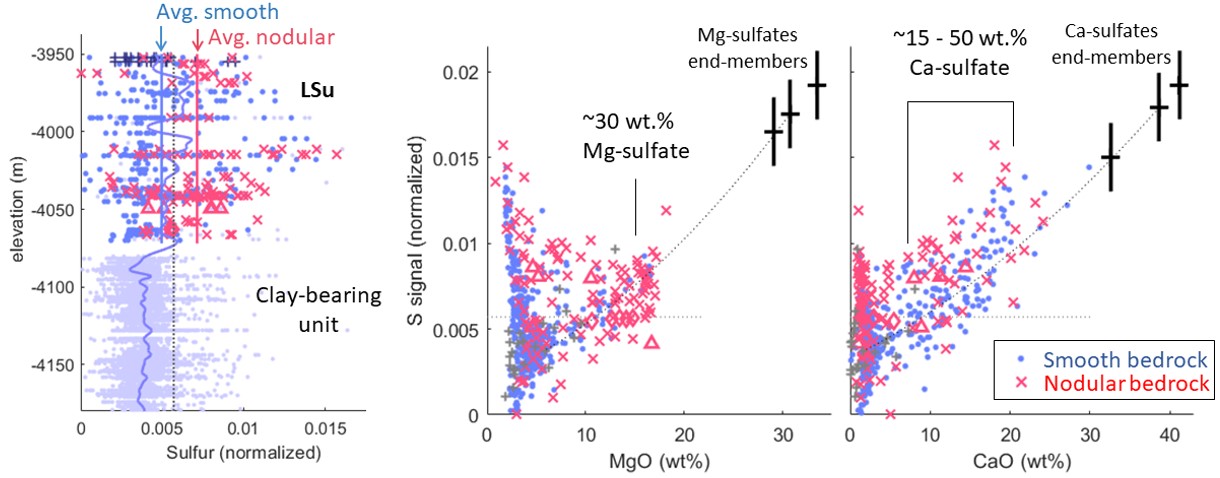
Figure 2: Top Geochemical transition into the sulfate-bearing unit as recorded by the ChemCam instrument on bedrock with both host and nodular textures. From left to right: Normalized sulfur signal on bedrock targets with elevation within the clay-bearing unit, the LSu, blue line shows bedrock average (host and nodular) highlighting a significant change of bedrock sulfur composition associated with the nodular bedrock (red line average); Sulfur as function of MgO and CaO content highlights the presence of Mg and Ca-sulfates in bedrock.
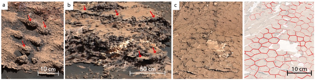
Figure 3: Remarkable nodular bedrock in the basal LSu highlights the diversity of textures observed within a short stratigraphic range with distinct sulfate-enriched composition. Decimeter-sized concretions (a); dark-toned nodular beds (b); regular pattern of polygonal ridges (c).
How to cite: Rapin, W., Sheppard, R., Dromart, G., Schieber, J., Clark, B., Kah, L., Rubin, D., Ehlmann, B., Gupta, S., Caravaca, G., Mangold, N., Dehouck, E., Le Mouélic, S., Gasnault, O., Clark, J., Bryk, A., Dietrich, W., Lanza, N., and Wiens, R.: The Curiosity rover investigates an aridification sequence in the layered sulfate-bearing unit., Europlanet Science Congress 2022, Granada, Spain, 18–23 Sep 2022, EPSC2022-1112, https://doi.org/10.5194/epsc2022-1112, 2022.
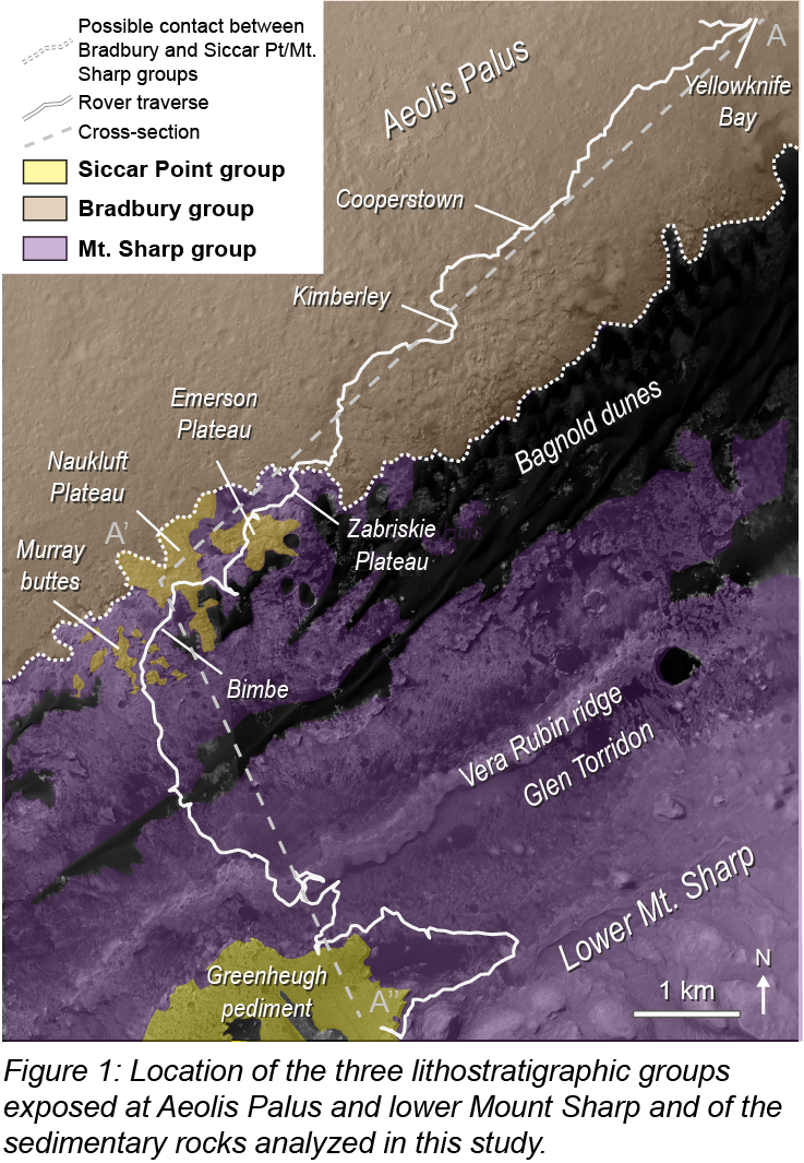
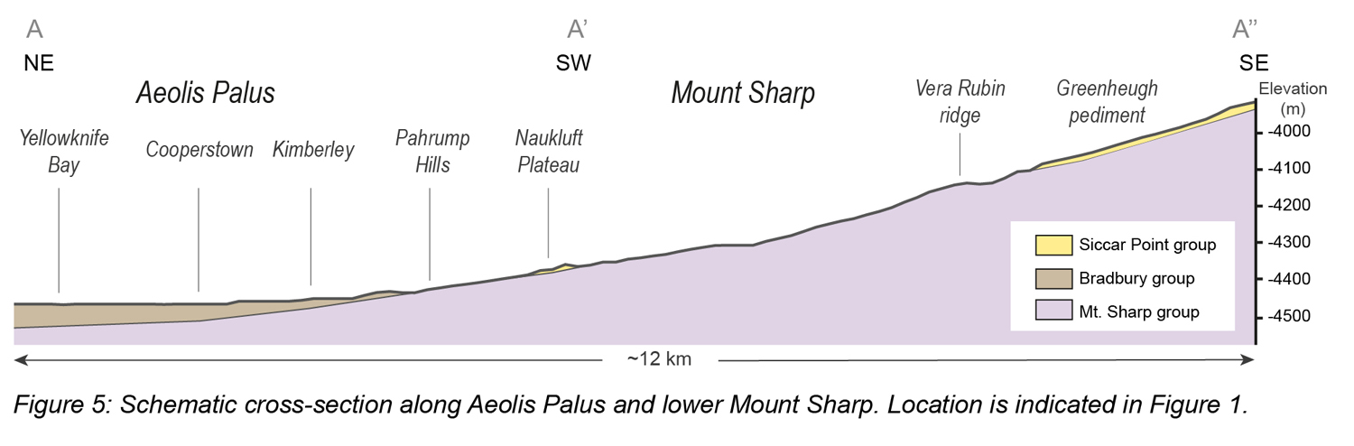
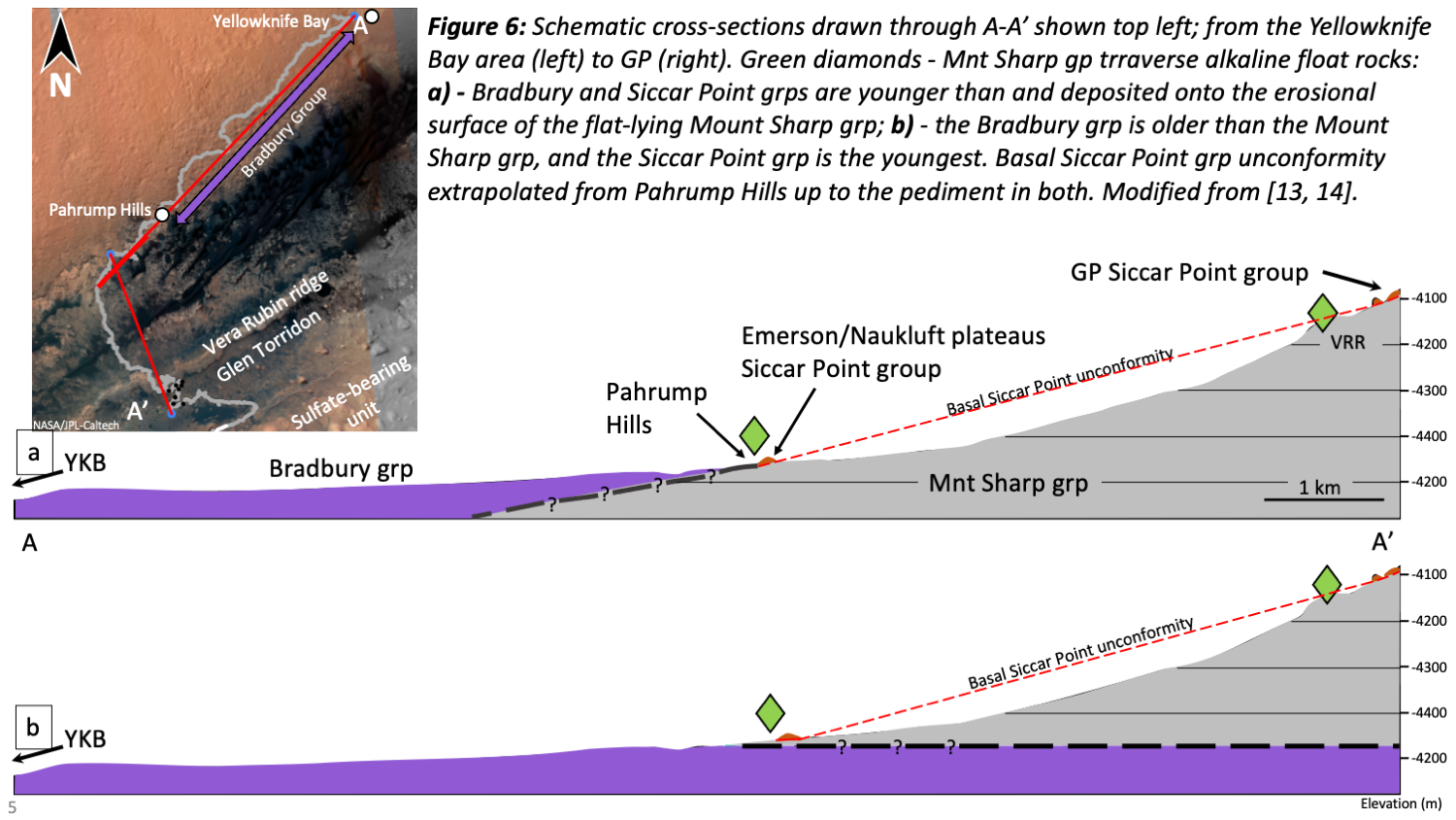
Over the past 10 years, the Mars Science Laboratory (MSL) rover Curiosity has been investigating the plains of Aeolis Palus and the lower reaches of Aeolis Mons (informally known as Mount Sharp), a 5 km tall mound of sedimentary rocks in Gale crater (Figure 1). After traversing 27 km and nearly 600 m of vertical stratigraphy, three lithostratigraphic groups have been identified: Bradbury, Mount Sharp, and Siccar Point (SP). The Bradbury group consists of fluvial, deltaic, and lacustrine sedimentary rocks [1-2]. The Mt. Sharp group mainly consists of laminated mudstones with minor fluvial sandstones, interpreted as evidence of a long-lived lacustrine environment [1]. Locally, exposures of the Mt. Sharp group are unconformably overlain by aeolian cross-bedded sandstones of the SP group, interpreted to have deposited on an aeolian deflation surface [3].
While these three groups show evidence of deposition in specific environmental and climatic conditions, knowledge of their stratigraphic relationships is a key information to understand the evolution of environmental conditions in Gale. Yet, no clear stratigraphic contact has been observed at the boundary between the Bradbury and the Mt. Sharp groups. Because the mean dip of the Bradbury group is approximately horizontal, the MSL team suggested that the Bradbury group might be stratigraphically lower than the Mt. Sharp group, and therefore lower than the SP group [1]. Nonetheless, orbital analyses of the region suggested that capping strata of the Bradbury group could be part of the SP group [4]. Chemical data from the ChemCam and APXS instrument suites of Bradbury and SP group rocks have recently shown that both groups have similar compositions and possibly similar sediment sources [5-8]. In this study, we aim to reappraise the stratigraphic and chemical relationships between the Bradbury and SP groups using Mastcam [9-10] and ChemCam data [11-12] to characterize the evolution of Gale’s ancient environment.
Lithostratigraphy of Zabriskie Plateau
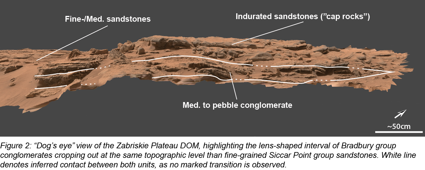
One of the best candidates to assess the potential contact between Bradbury and SP group rocks is located at the Zabriskie Plateau outcrop in the Pahrump Hills area (Figure 1). To better appreciate the facies and 3D geometry of the contacts, this outcrop has been reconstructed as a Digital Outcrop Model (Figure 2, https://skfb.ly/o9ZAq) [13]. In this model, we observe that most of the outcrop is composed of fine to medium-grained sandstones, arranged in dm- to meter-scale cross-stratifications, similar to some of the aeolian facies of the SP group [3]. These sandstones exist as “capping rocks” similar to previously described examples [4], suggesting that they are locally well-cemented on the topmost meter. Near the base of the DOM, we observe a meter-scale, ~30-cm thick, cross-stratified lens-shaped interval of coarser medium to pebble conglomerate. This level represents deposition under energetic aqueous conditions to transport clasts up to the pebble size, more likely to pertain to a fluvial channel. Interestingly, this conglomerate interval is at similar elevation (within one meter) to the surrounding sandstones, with no apparent unconformity, likely evidencing a conformable emplacement of this level within the finer sandstone succession. This would argue that the conglomerate level was deposited synchronously with the finer-grained sandstones during the same depositional event.
Chemical composition of Bradbury and Siccar Point groups
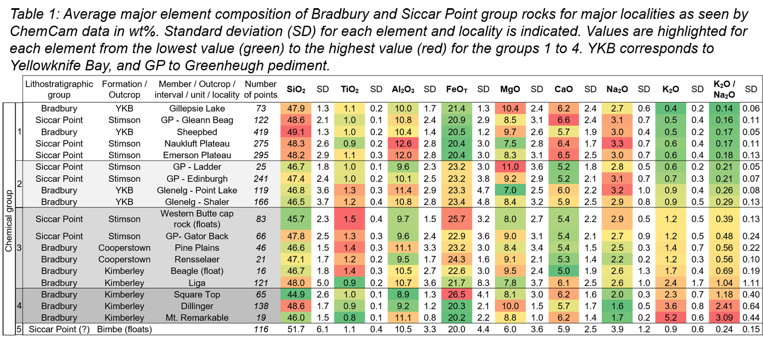
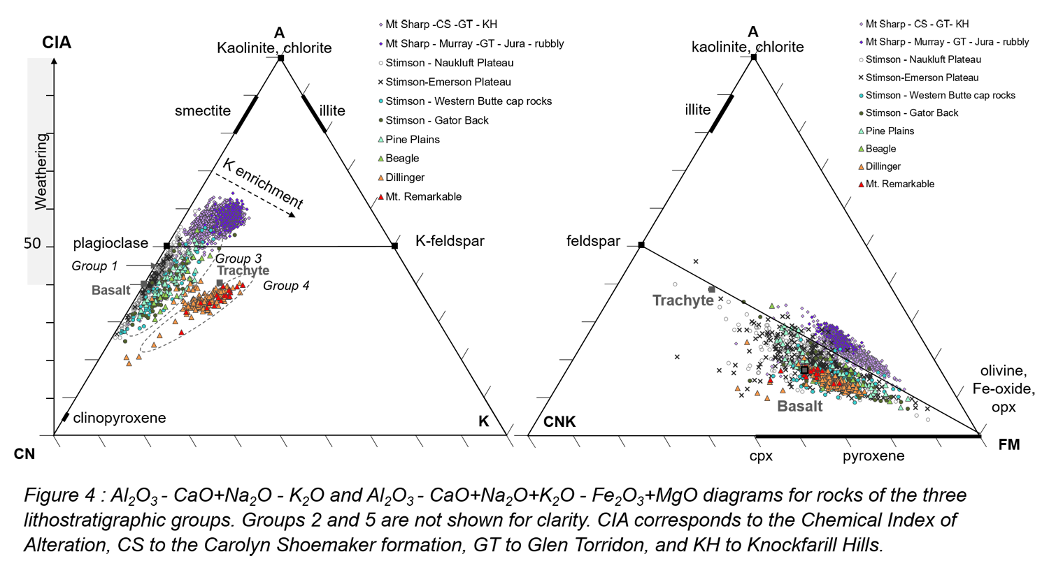
The average compositions of Bradbury and SP group rocks are overall quite similar (Table 1), and clearly distinct from Mount Sharp group rocks (Figures 3 and 4). By analyzing the rock compositions of Bradbury and SP groups, we sorted them into five major chemical groups, which are, in order of increasing average K2O/Na2O ratio and average K2O content for groups 1 to 4: group 1 has a basaltic composition; group 2 has low SiO2, intermediate TiO2, high FeOT and Na2O contents; group 3 has low CaO, high TiO2, FeOT, and K2O contents; group 4 has low TiO2 and Al2O3, and very high K2O contents; and group 5 has a composition close to group 1 with higher SiO2 and alkali contents (Table 1, Figure 3). Overall, the MgO and Al2O3 contents are quite variable. The composition of these rocks suggests mixing between mafic minerals and feldspars, including alkali feldspars in various proportions (Figure 4). Interestingly, both Bradbury and SP rocks occur in the first three chemical groups, which suggests similar source rocks for both groups of at least two types: a relatively low-potassium basaltic rock and a potassic-rich rock. The relative abundance of potassic-rich source rock in the mixture is interpreted to increase from group 1 to group 4. Besides, Bradbury and SP group rocks have a low Chemical Index of Alteration (CIA), which is indicative of limited chemical weathering (Figure 4).

Conclusion
3D observations in the Pahrump Hills area suggest that Bradbury and Siccar Point units are intermingled and synchronous in an environment allowing fluvial episodes to occasionally occur among a drier setting, as observed on Earth [14]. This is consistent with the chemical compositions of Bradbury and Siccar Point groups which suggest similar source rocks in different relative abundances. This relationship implies that the Bradbury group could be younger than Mount Sharp group (Figure 5). To summarize, these observations are in favor of a common origin for both Bradbury and Siccar Point as a single clastic group, representing a temporal evolution from clement conditions during the deposition of Mount Sharp group to a colder and drier environment with still transient episodes of fluvial activity during the deposition of Bradbury and Siccar Point groups.
[1] Grotzinger et al., Science 2015. [2] Mangold et al., JGR 2016. [3] Banham et al., Sedimentology 2018. [4] Williams et al., Icarus 2018. [5] Bedford et al., Icarus 2020. [6] Bedford et al., JGR 2022. [7] Thompson et al., LPSC 2022. [8] Thompson et al., this conference. [9] Malin et al., LPSC 2010. [10] Bell et al., Earth and Space Science 2017. [11] Wiens et al., Space Sci Rev. 2012. [12] Maurice et al., Space Sci. Rev. 2012. [13] Caravaca et al., PSS 2020. [14] Newell, Marine and Petroleum Geology 2001.
How to cite: Le Deit, L., Caravaca, G., Mangold, N., Le Mouélic, S., Dehouck, E., Bedford, C. C., Wiens, R. C., Johnson, J. R., Gasnault, O., Forni, O., and Lanza, N.: Investigation of the stratigraphic and chemical relationships between Bradbury and Siccar Point lithostratigraphic groups in Gale crater, Mars, Europlanet Science Congress 2022, Granada, Spain, 18–23 Sep 2022, EPSC2022-508, https://doi.org/10.5194/epsc2022-508, 2022.
Introduction:
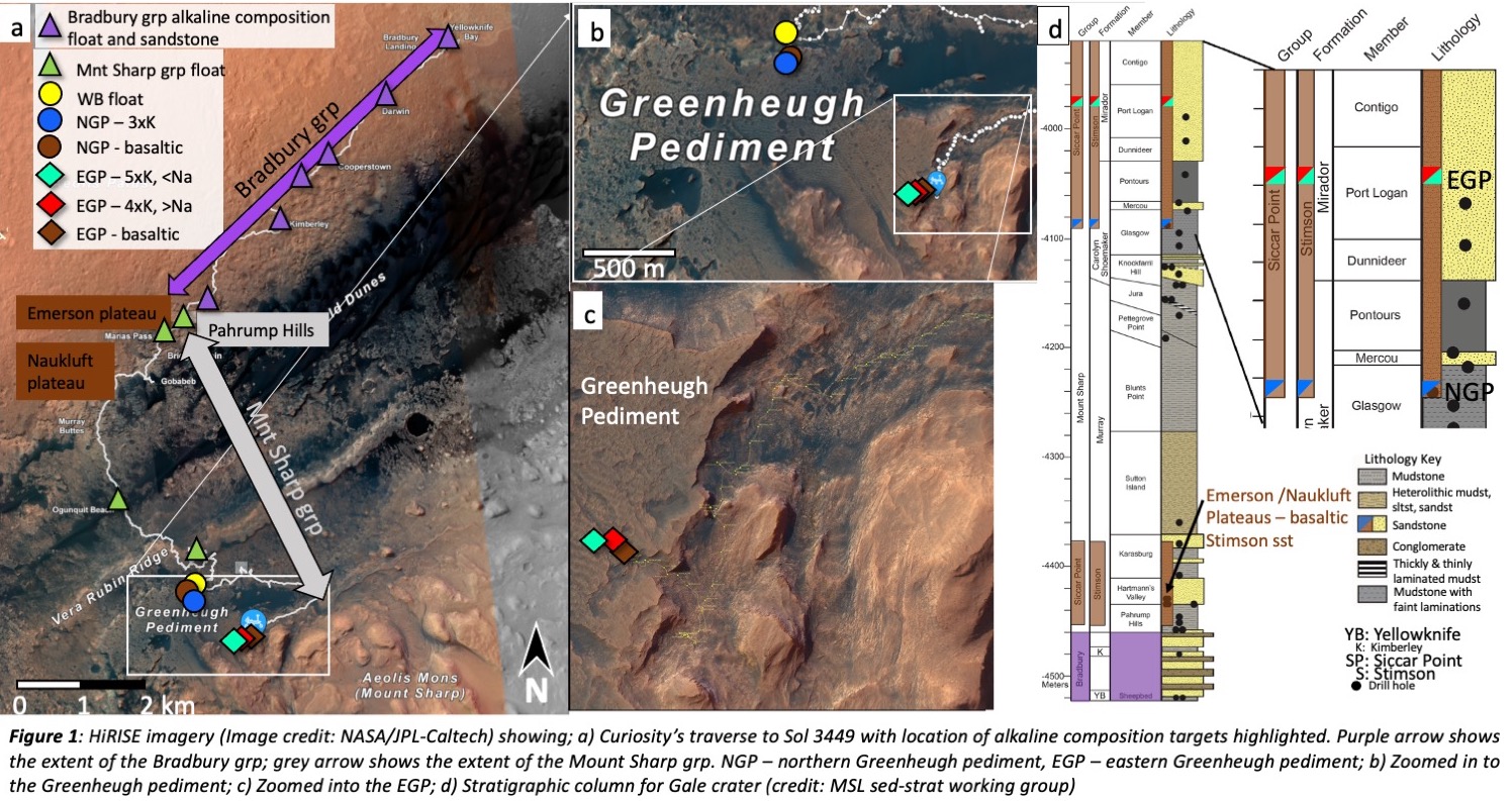
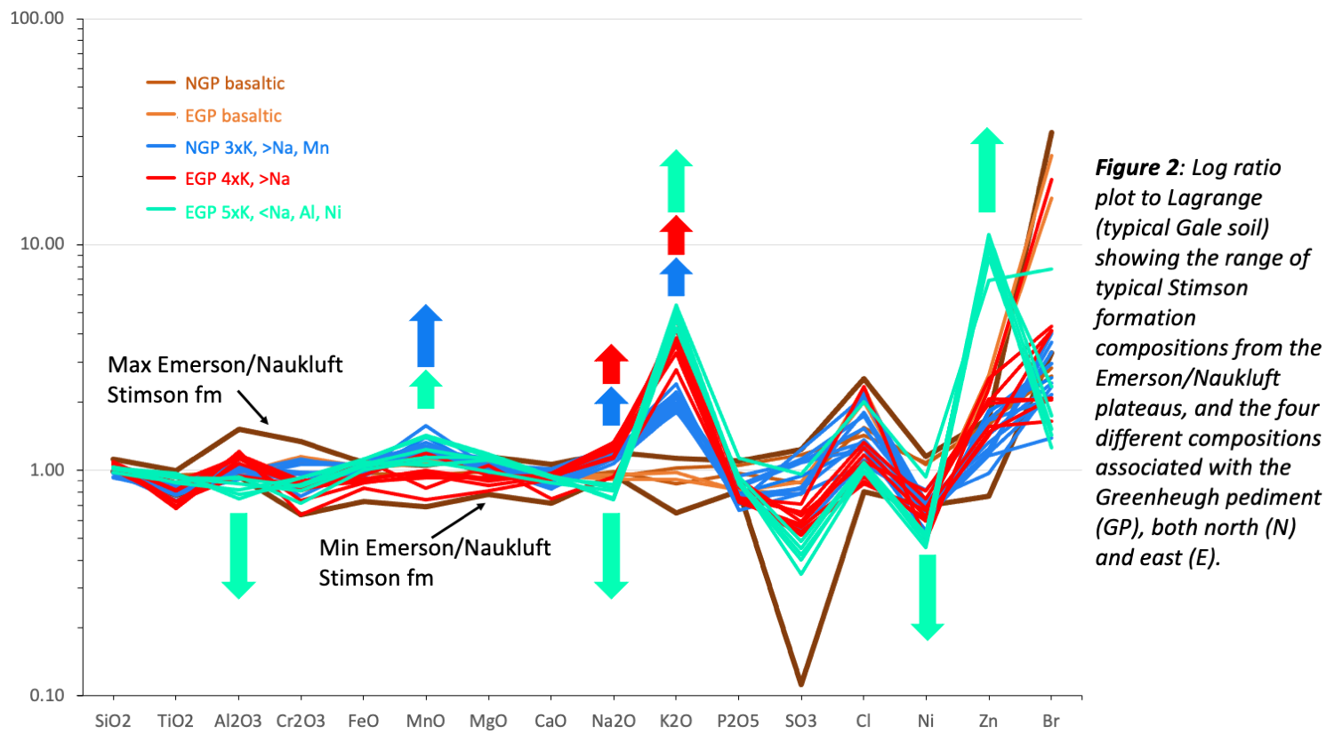
Curiosity has encountered eolian Stimson formation, Siccar Point group sandstones [1-3] at several locations during ascent of Mount Sharp, Gale crater, at: 1) the Emerson and Naukluft plateaus; 2) on the northern Greenheugh pediment (GP); and most recently 3) on the eastern GP (Figure 1). The Siccar Point group unconformably overlies [4] the predominantly lacustrine, Mount Sharp group, which itself is considered to overlie the Bradbury group (Figure 2). Alpha Particle X-ray spectrometer(APXS) analyses acquired during recent investigations of the eastern GP have expanded the range of eolian Stimson formation compositions and provide further evidence for a relationship with Bradbury group sandstones and cap rocks encountered early in the mission. The Bradbury group includes alkaline composition sandstones, clasts within breccio-conglomerates, and float rocks interpreted to represent primary igneous and volcaniclastic rocks derived from mixing of multiple igneous source rocks [5-12]. We report the results of APXS analyses of the Stimson formation and discuss implications for provenance and timing of events within Gale crater.
APXS results:
Basaltic composition sandstones, related to average Mars sand and soil, were identified at all three Stimson locations (Figures 1,2). All compositions are discussed here, relative to typical basaltic Stimson chemistry. Sandstones with 3xK2O and >MnO concentrations are identified on the northern GP overlying basaltic composition sandstones (Figures 1,2) [13-14]. Most recently, on the eastern GP, APXS analyses have revealed sandstones with even >K2O concentrations that fall into two groups (Figures 1,2): 1) with ~4xK2O, trending to >Na2O concentrations, and 2) with ~5xK2O, trending to <Na2O, Al2O3, and Ni, ≫Zn and Ge, and ≈MgO concentrations. The eastern GP, high-K sandstones also overlie more typical basaltic chemistry sandstones.
Compositional relationship to Bradbury group and other targets previously encountered on the mission:
The higher-K, Stimson sandstones share many compositional characteristics with Bradbury group rocks as well as several float rocks encountered along the Mount Sharp group traverse [13-14] (Figures 3,4). The CCAM instrument has also detected similar relationships [15]. The Bradbury group targets include sandstones near the landing site, high-K Bathurst and Kimberley formation sandstones, and capping sandstones situated just prior to driving on to the Mount Sharp group. Related composition float rocks analyzed along the Mount Sharp traverse are typically associated with Stimson outcrops.
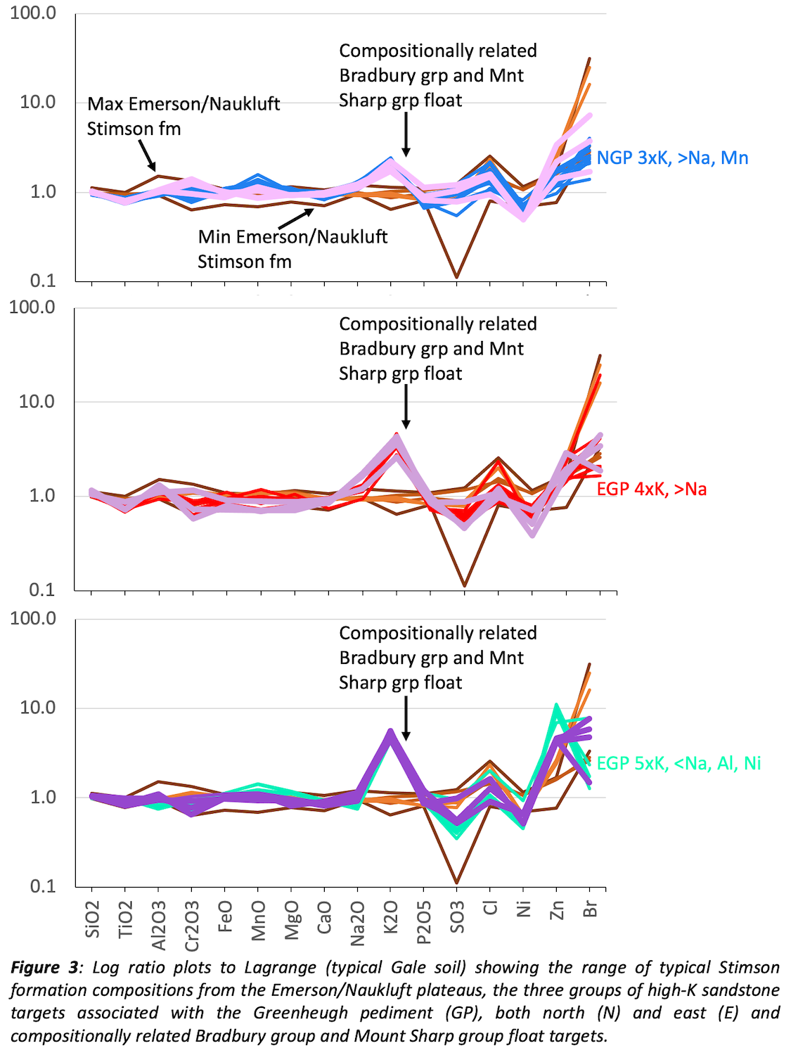
The higher-K Stimson sandstones do not plot on the sorting trend defined by the varying grainsize, modern Gale crater sands, and the basaltic Stimson sandstones on an A-CN-K diagram (Figure 4b). Instead, they are offset parallel to the plagioclase–potassium feldspar join. Thus, we do not attribute the compositional differences between the basaltic and high-K pediment Stimson to be the result of eolian sorting. Instead, based on sedimentology [3], mineralogy [16], and composition [13-14], we invoke a change in provenance, with input of a more potassium feldspar-rich source. Given the compositional relationship to Bradbury group sandstones, we suggest that the high-K Stimson sandstones are also derived from the mixing of multiple, igneous source rocks including basaltic and more alkaline compositions [13-14].
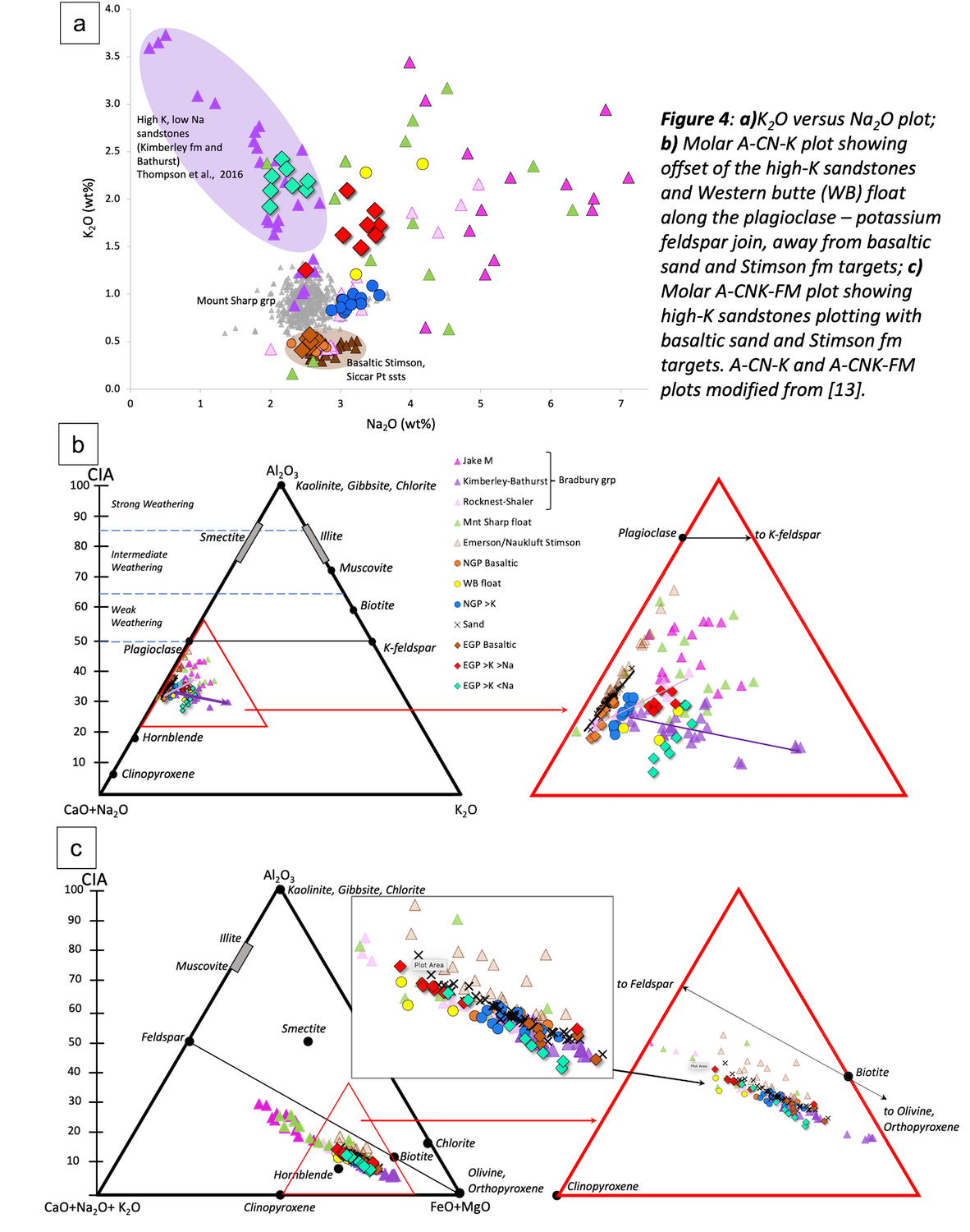
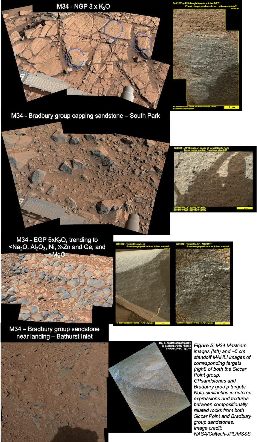
Many of the Bradbury group sandstones, Mount Sharp float and higher-K, pediment sandstones are also texturally alike. They are all relatively smooth, resistant, and blockier in appearance than typical basaltic Stimson sandstone (Figure 5). The high-K pediment and Bradbury sandstones also share similar orbital characteristics; both are manifest as crater-retaining units.
Timing Implications:
The more alkaline composition Bradbury group sandstones near the landing site are >9 km lateral distance and 400 m of elevation from the high-K pediment sandstones. Therefore, we have found evidence along the entire traverse for the presence of alkaline igneous source rocks. These source rocks have provided sediment input to both fluvial (Bradbury) and eolian (Siccar Point) sandstones [13-14]. Based on the compositional and textural relationships between the Bradbury and Siccar Point groups we revisit the timing of events at Gale.
The Bradbury group is generally considered to be older than both the Mount Sharp and Siccar Pt groups (Figure 1). This work raises the possibility that they could instead be contemporaneous, with both being younger than the Mount Sharp group. In this scenario, the Mount Sharp group represents relatively old lacustrine/fluvial deposits, which were buried, lithified, and eroded, before deposition of the Bradbury and Siccar Point groups onto that erosional surface, thus explaining differences in elevation between the two groups (Figure 6a). Alternatively, the Bradbury group alkaline sedimentary rocks are the oldest unit and would have been deposited prior to the Mount Sharp group. The Siccar Point group eolian sandstones (basaltic and alkaline) would then have been deposited on to the Mount Sharp group (Figure 6b). In this case, a more alkaline source area in the vicinity of, or within, Gale crater has been eroded by both water and wind at different times during the history of the evolution of the crater and its infill [13-14]. Both scenarios are consistent with widespread evidence at Gale crater for the presence of multiple igneous source rocks.
Acknowledgements:
MSL APXS is managed and financed by the Canadian Space Agency (CSA). Thanks to the JPL engineers and MSL science team.
References:
[1] Banham, S.G., et al. (2018) Sedimentology, 65, 993–1042. doi.org/10.1111/sed.12469
[2] Banham, S.G., et al. (2021) JGR: Planets, 126 (4): e2020JE006554
[3] Banham, S.G., et al. (submitted) JGR: Planets
[4] Watkins, J.A., et al. (2016) 47th LPSC, Abstract #2939
[5] Stolper, E.M., et al. (2013) Science 341 (6153), 1239463. doi:10.1126/science.1239463
[6] Schmidt, M.E., et al. (2014) JGR Planets, 119(1):64-81, doi:10.1002/2013JE004481
[7] Sautter, V., et al. (2015) Geoscience, 8(8), 605.
[8] Thompson, L.M., et al. (2016) JGR Planets, 121(10):1981-2003, doi:10.1002/2016JE005055
[9] Treiman, A.H., et al. (2016) JGR Planets, 121(1), p.75 – 106. doi:10.1002/2015JE004932
[10] Cousin, A., et al. (2017) Icarus 288, 265-283. doi:10.1016/j.icarus.2017.01.014
[11] Edwards, P.H., et al. (2017) MAPS, 52 2931-2410. doi.org/10.1111/maps.12953
[12] Bedford, C.C., et al., (2019) Geochimica et Cosmochimica Acta, 246, 234-266. doi.org/10.1016/j.gca.2018.11.031
[13] Thompson, L.M., et al., (submitted) JGR Planets 2021JE007178
[14] Thompson, L.M., et al., (2022) 53rd LPSC, 1475.pdf
[15] LeDeit, L., et al. (this conference)
[16] Thorpe, M.T., et al. (Submitted) JGR Planets 2021JE00709
How to cite: Thompson, L., Spray, J., Gellert, R., Williams, R., Berger, J., O'Connell-Cooper, C., Yen, A., McCraig, M., VanBommel, S., and Boyd, N.: APXS-determined compositional diversity of eolian Siccar Point group sandstones, Gale crater Mars: Implications for provenance and timing of events, Europlanet Science Congress 2022, Granada, Spain, 18–23 Sep 2022, EPSC2022-1184, https://doi.org/10.5194/epsc2022-1184, 2022.
NASA’s Mars 2020 Perseverance rover mission is seeking signs of ancient life in Jezero crater and is collecting a cache of Martian rock and soil samples for planned return to Earth by a future mission. A key exploration target for the mission is a prominent sedimentary fan deposit at the western margin of Jezero crater that has been interpretated to be a river delta that built into an ancient lake basin during the Late Noachian-Early Hesperian epochs on Mars (~3.6-3.8 Ga) [1, 2]. Long distance observations of a remnant butte (informally named Kodiak) related to the western fan demonstrated that it comprised two distinct Gilbert-type delta units [2, 3].
In her approach to the western fan, Perseverance drove alongside the east-facing scarp of the western fan and arrived at a key location called Three Forks - a setting off point for delta exploration - in April 2022. Images from the Mastcam-Z and SuperCam Remote Micro-Imager instruments provide new views of the stratigraphy exposed in the erosional front of the western Jezero delta; in particular, showing sections of the delta previously not visible from long distance observations and at much higher resolution. These observations provide the first direct evidence of delta geometries in the main western fan deposit. Here, we report its stratigraphy and sedimentology, which provide new constraints on the nature of the fan deposits, and therefore paleoenvironmental implications.
A Mastcam-Z mosaic of basal delta strata acquired on sol 411 in the vicinity of Three Forks and at an approximate distance of 250 m from the scarp provides a spectacular view of a prominent embayment in the delta scarp that has been informally named Hawksbill Gap. Hawksbill Gap is the proposed ascent route for Perseverance in her investigation and sampling of delta front strata. Prominent cliffs that make up the eastern and western margin of Hawksbill Gap show stratal patterns similar to those observed at Kodiak. The mid-sections of the scarps are characterized by decametre-scale inclined strata interpreted as foreset strata of a Gilbert-type delta succession. Internally these comprise stacked tabular beds that are locally conglomeratic but predominantly comprise finer-than-conglomerate lithologies, likely pebbly sandstones. Units with variable dips are present, together with some evidence of over-steepened dips suggestive of possible slumping or synsedimentary deformation. On the eastern side of Hawksbill Gap, the inclined strata are overlain across a sharp truncation surface by generally planar parallel thin-bedded horizontal strata that we interpret as topset beds deposited by fluvial processes in a delta top environment. The prominent erosion surface separating the foresets from the topsets indicates that these are oblique prograding clinoforms, which suggests delta progradation here during lake level fall based on Earth field examples and experimental studies. Conglomerate beds containing boulders are observed within the topset strata indicating sediment-transport on the delta top by episodic high-discharge floods. Their relationship to the delta-capping boulder conglomerates described by Mangold et al. 2021 that were interpreted as evidence for major post-delta flood episodes remains to be determined. Foreset beds capped by sub-horizontal topsets are also observed on the western flank of Hawksbill Gap. Observations of the western flank of Hawksbill Gap, interpreted to be a promontory of a preserved channel body show complex bivergent inclined stratification indicative of a complex delta geometry, possibly a very narrow (~200 m wide) lobe distinct from other lobes of the delta. Detailed analysis of such stratigraphic patterns will permit reconstruction of fine-scale depositional processes and preservation here.
The Sol 411 Mastcam-Z mosaic from Three Forks also revealed the basal stratigraphy of the Jezero western delta for the first time showing low relief, recessive strata separated by laterally continuous at 100 m scale, thin tabular resistant beds that provide useful local marker horizons to sub-divide the stratigraphy. On a ledge at the top of lowermost strata, a distinct very light-toned layer that is laterally continuous for tens of metres is observed in the Mastcam-Z mosaic (and also in HiRISE imagery). This distinct unit has been informally named at two locations as Hogwallow Flats and White Rocks. Above Hogwallow Flats a prominent resistant planar unit that forms a distinct planar unit named Rocky Top is visible in Mastcam-Z and HiRISE imagery. This unit in vertical section has thin-bedded strata in its lower part and more thickly bedded at its top which may represent a thickening-up succession typical of lobe progradation in delta toe settings. This unit is laterally discontinuous clearly pinching out to the east and disappearing within less resistant beds.
In the light of the occurrence of horizontally bedded strata at the base of the delta scarp and also located below, the horizontally bedded basal strata below the large-scale inclined strata interpreted as foreset beds may represent bottomset and delta toeset beds. In this scenario, the more resistant beds may represent coarser-grained turbidite flow deposits, with the less resistant strata perhaps representing finer-grained rocks that weather more recessively. The latter may have formed from either fine-grained turbidity currents or decantation processes in a prodelta environment. Close range observations are required to test these hypotheses.
Interrogation of the stratal geometry and sedimentary facies of the western delta succession will provide constraints on the character, relative timing and persistence of ancient aqueous activity at Jezero. Such analyses inform interpretations of Martian climate evolution, potential habitability, and search strategies for rocks that might contain potential biosignatures and organic matter.
References: [1] Goudge et al. (20170 EPSL doi:10.1016/j.epsl.2016.10.056
[2] N. Mangold, et al., (2021) Science, 10.1126/science.abl4051.
[3] Caravaca et al, (2022) EPSC this meeting.
How to cite: Gupta, S. and the NASA Mars2020 science team: Sedimentary and stratigraphic observations at the Jezero western delta front using Perseverance cameras: initial constraints on palaeoenvironments, Europlanet Science Congress 2022, Granada, Spain, 18–23 Sep 2022, EPSC2022-1098, https://doi.org/10.5194/epsc2022-1098, 2022.
Introduction:
The Perseverance rover landed at Jezero crater in 2021, close to the delta of an ancient river (1). This crater once hosted a paleolake (2). Previous studies of this system have concluded that the current fan-delta units were formed during the last phase of the Jezero fluvial activity, which postdates the formation of the olivine-rich unit and predates the formation of the current floor unit. From crater counts, the formation of the delta unit is assigned to an Early or Late Hesperian age (3.5 + 0.1/-0.3 Gy) (3). However, little is known about the processes that happened before and the plausible fluvial and igneous history that determined the evolution of the fresh impact crater. A comparative analysis with craters of similar size suggests that Jezero crater has experienced approximately 1 km of infilling compared to the morphologically fresh crater(4,5). The crater floor depth d can be calculated with the power-law scaling d = 0.372D0.375 + 0.072D0.62 (6) , which is valid for craters wider than 7 km. For Jezero D=49 km and the crater floor base should be at a depth of 2,404 m.
The purpose of this work is to investigate the plausible existence of preserved radar reflectors (7–12) that may indicate the geometry of crater filling layers. Recent research by other authors (7) have confirmed the usefulness of this approach to detect preserved layers in other craters. Here we shall apply a similar methodology to investigate it on Jezero crater.
Materials and methods:
SHARAD is a sounding radar experiment aboard the MRO mission designed to reveal the shallow structures of the Martian subsurface.(9). We visualize SHARAD radargrams using JMARS software. When a potential echo is detected as a bright feature, these signals have to be compared with the simulated cluttergrams, that are produced using the current surface topography, (MOLA-HRSC with 200m/pix. and MOLA with 463m/pix) in order to discriminate ghost signals. The protocol followed to investigate the plausible existence of buried reflectors on MARS using SHARAD data is the following one:
- Interpret visually the radargrams looking for subsurface reflectors in JMARS.
- Download the geometry data for each radargram under investigation and crop only the area of study, to reduce the computational time.
- Build the clutter simulation using the sets of topography data mentioned above. The data were downloaded from astrogeology. The DTM was selected only for the area of interest to reduce the overall computational resources. The clutter simulator estimates the reflected echoes from the topography based on the directivity pattern of the antenna, the distance from the source, and the orientation of the slope with respect to the angle of incidence (13)
- Compare the off-nadir reflections with the apparent bright reflectors.
- If a true reflector is detected, the wave travel times can be transformed to depth using Δh=c Δt/√ε where ε is the assumed permittivity of the materials above the reflector.
In order to test our methodology we validate it in a previously described case, in a crater near Mangala Fossa region (7). A confirmed reflector, which is distinguished in the radargram underneath the subsurface (Fig1-b) is not seen in the cluttergram (Fig1-a) confirming it as a true buried reflector. Any other bright feature that appears in both images is an artifact produced by the radar echo of the surface.
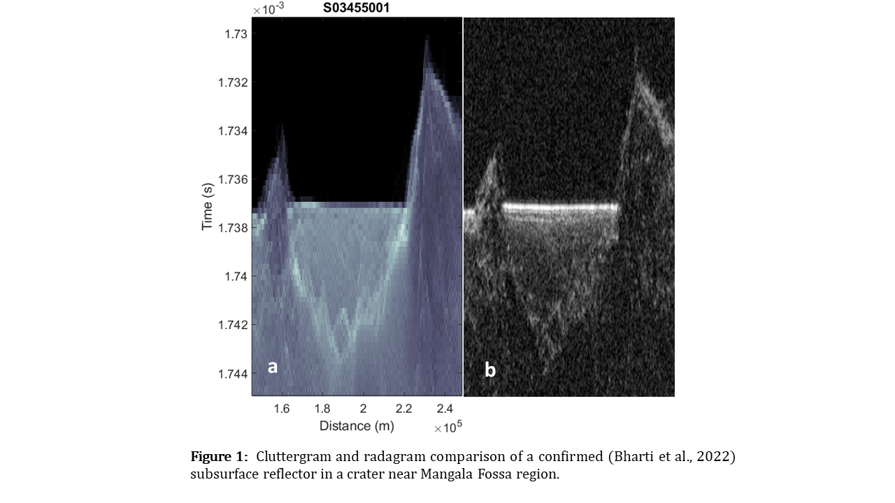
Next we apply this methodology to Jezero crater. We observe in Figure 2-b an example of a potential reflector. To confirm or discard the nature of this reflector we compare with the cluttergrams at different resolution scales, in Figure 2-a and 2-c. The reflectors from SHARAD data are observed on the radagrams at both resolution scales and therefore they are interpreted as artifacts produced by surface topographic echoes. Similar examples are shown in Figures 3 and 4.
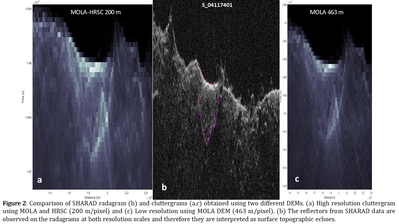
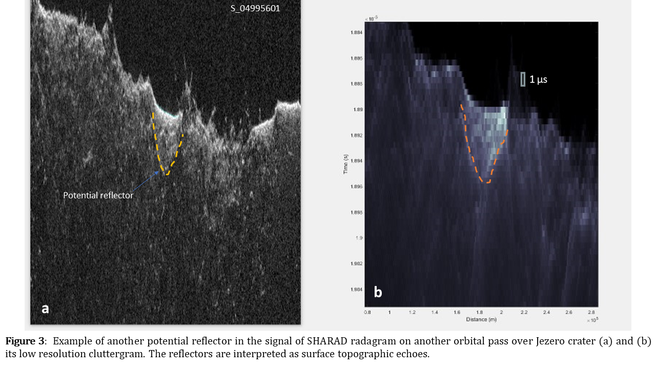
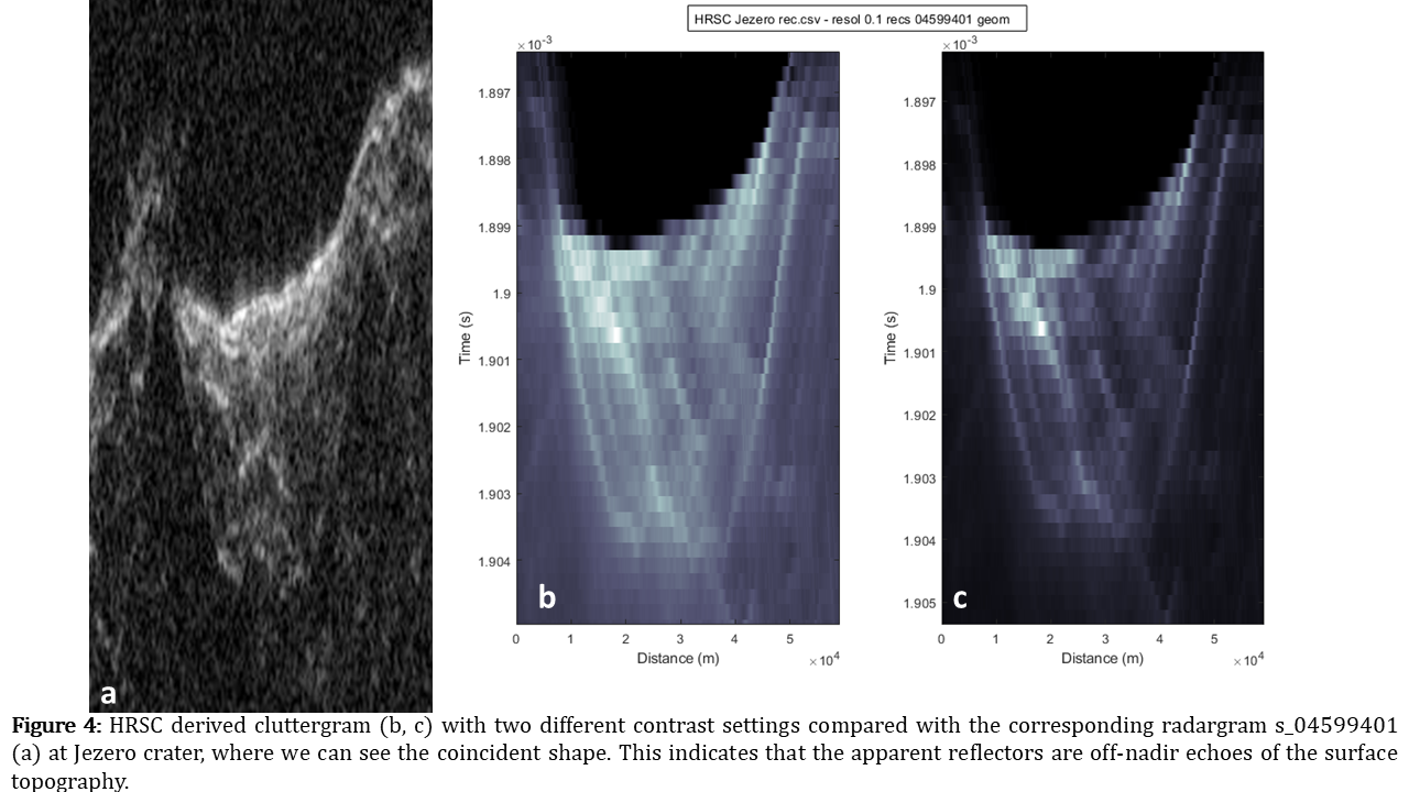
Conclusions:
Our preliminary analysis, can discard the existence of true recognizable reflectors at Jezero. Assuming ε= 6 (14) and a crater filling depth of about 1 km, a crater-base reflector should have given an echo at a single travel time less or equal than 8165 ns. This distance is covered in our investigation and therefore this analysis suggests that SHARAD measurements can neither detect any reflector within the crater filling nor distinguish the crater floor. This may be due to the presence of strong off nadir reflections produced by the surface topography that may overwrite true reflectors. Moreover, gradual variations between layers can reduce their reflection coefficients making them transparent to radar. Future studies will investigate the existence of subsurface reflectors in environments with higher signal to clutter ratio, such as paleolake environments with smoother surfaces.
Acknowledgments: We are grateful to the PDS, SHARAD and HRSC for the materials and JMARS and QGIS for the software. The work of F. Mansilla is supported by the grant PRE2020-09170 founded by MCIN/AEI/10.13039/501100011033. Spanish State Research Agency (AEI) Project No. MDM‐2017‐0737 Unidad de Excelencia “María de Maeztu”‐ Centro de Astrobiología (INTA‐CSIC) and the Spanish Ministry of Science and Innovation (PID2019‐104205GB‐C21).
References:
- N. Mangold et al., Science. 374, 711–717 (2021).
- C. I. Fassett, J. W. Head, Geophys. Res. Lett.32, 14, (2005)
- N. Mangold et al., Astrobiology. 20, 994–1013 (2020).
- S. C. Schon, et al., Planet. Space Sci. 67, 28–45 (2012).
- B. D. Boatwright, J. W. Head, Planet. Sci. J. 2, 52 (2021).
- L. Pan, et al., Nat. Commun. 10, 4257 (2019).
- R. R. Bharti, et al., Icarus. 371, 114713 (2022).
- I. Ganesh, L. M. Carter, I. B. Smith, J. Volcanol. Geotherm. Res. 390, 106748 (2020).
- R. Seu et al., J. Geophys. Res., 112, E5 (2007).
- M. N. Simon, et al., J. Geophys. Res. Planets. 119, 2291–2299 (2014).
- T. R. Watters et al., Science. 318, 1125–1128 (2007).
- S. Xiong et al., Earth Space Sci. 8 (2021).
- P. Choudhary, et al., IEEE Geosci. Remote Sens. Lett. 13, 1285–1289 (2016).
- S. Eide, et al., IEEE J. Sel. Top. Appl. Earth Obs. Remote Sens. 14, 2484–2493 (2021).
How to cite: Mansilla, F., Zorzano, M. P., Giannakis, I., and Ruiz, J.: No evidence of reflectors on Jezero radargrams, Europlanet Science Congress 2022, Granada, Spain, 18–23 Sep 2022, EPSC2022-460, https://doi.org/10.5194/epsc2022-460, 2022.
Introduction: Mars is a primary destination to search for signs of life and probing the subsurface is a key element in this search. Access to the Martian subsurface, under most altered layers, is needed to understand the nature, timing and duration of alteration and sedimentation processes on Mars, as well as habitability conditions. For such a reason, ExoMars rover mission includes a drill to collect subsurface samples and has a complex payload able to conduct detailed investigations of composition, search for organics, and recognize indicators of past or extant life[1]. The drill is a critical element of the mission which will explore and collect samples down to 2 m of depth. An essential part of the payload is Ma_MISS (Mars Multispectral Imager for Subsurface Studies) experiment hosted by the drill system[2,3]. Ma_MISS is a Visible and Near Infrared miniaturized spectrometer with an optical head inside the drill tip capable of observing the borehole from where samples are collected.
Ma_MISS instrument description: Ma_MISS miniaturized spectrometer is hosted inside the drill system of the ExoMars rover and will characterize the mineralogy and stratigraphy of the excavated borehole wall at different depths (up to 2 m).
|
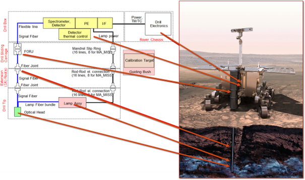
Ma_MISS is a modular instrument, and it consists of two main parts: (i) the spectrometer with the PE located outside of the drilling tool, and (ii) the Optical Head (OH) and fibers located inside the drill itself (Fig.1). The Drill consists of a main rod and three additional rods to reach a maximum depth of 2 m. The drill tip also has the Ma_MISS OH with a sapphire window to observe the borehole wall. All the rods are equipped with optical fibers to transmit light and signal. Ma_MISS is equipped with a light source of 5W and the illumination spot is about 1 mm at a focal distance of about 0.6 mm. The reflected light is collected through a 120 μm spot. The spectrometer observes a single point on the borehole wall and, using the drill movements, can build up images of the target. By combining several column and ring observations, Ma_MISS allows the reconstruction of a complete image of the borehole wall (Fig.2). Ma_MISS spectral characteristics and fine spatial resolution enable the in situ investigation of rocks, prior the sample collection, that will be manipulated and crushed for further analysis by the analytical laboratory. Thus, Ma_MISS is the instrument that will closely investigate the mineralogical characteristics of Mars subsurface material in its original geologic context.
|
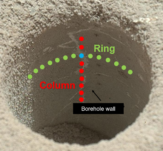
What mineralogy is expected in the subsurface ? Ma_MISS will investigate deeper into the subsurface than prior rover missions. Viking and Phoenix landers scooped materials from the upper few centimeters for compositional analysis. The MER excavated trenches up to 11 cm deep[4] and collected data with the alpha-particle x-ray spectrometer and Mossbauer instruments. The MERs [5] grounded up to 9 mm deep and revealed coatings enriched in S, Cl, Zn and Ni and iron oxides on outer rock surfaces. The MER data from the subsurface show that those soils had high ferric sulfate contents or silica contents, likely signaling an influence from volcanic or hydrothermal processes[6,7]. Mars Science Laboratory (MSL) drilled several holes into the Martian surface demostraing differences between the surface and the subsurface, as shown in the colors of the excavated fines, mainly linked with the oxidation state of the materials[8]. Most interesting is the fact that well preserved organic material was discovered at Pahrump Hills , even with the very harsh surface conditions, suggesting even better preservation may be possible farther beneath the Martian surface[9].
Differently from the previous missions, the drill and Ma_MISS measurements will be the deepest compositional measurements made on Mars. Ma_MISS is able to detect compositional gradients with depth, changes in type and abundance of minerals, weathering fronts or rinds, and diagenetic veins or nodules. The spectral range of Ma_MISS is optimal to detect changes in the occurrence and crystal chemistry of olivines and pyroxenes as well as Fe(II)/Fe(III) in silicates, oxides, and salts. There may be changes in these redox sensitive minerals with depth that record different environments. Furthermore, changes in the hydration state of materials can be also detected. For Oxia, the study of the subsurface could provide information on depositional regimes in zones not too far from the delta deposits, using the granulometric variation with dept.This will help to reconstruct the paleoenvironments that have characterized Oxia Planum.
In addition, at sufficient concentrations, organic molecules will also be detectable [10]: depending on the kind of organic, Ma_MISSis capable to detect their presence even when a 1 wt.% in the mixture, as verified by specific tests in the laboratory using the Ma_MISS breadboard. Spectroscopic measurements on these mineral/organic mixtures are useful to understand how the Ma_MISS instrument can detect traces of organic intimately mixed with minerals.
Conclusion: Ma_MISS will reconstruct the 3-D images of the borehole excavated by the ExoMars drill and will acquire spectra of the subsurface layers from which the sample will be collected. The calibration and tests performed with the flight model demonstrate the ability of the instrument in detecting most of the spectral signatures expected in Martian subsurface, including those due to the presence of possible salts and organics.
Acknowledgments. This work is fully funded and supported by the Italian Space Agency (ASI) [Grant ASI-INAF n. 2017-48-H.0].
References. [1] Vago et al. (2017) Astrobiology 17, 471–510. [2] De Sanctis, M. C. et al. (2017) Astrobiology, 17(6–7). [3] De Sanctis et al. (2022) PSJ in press. [4] Sullivan, R., et al.. (2011), J. Geophys. Res., 116, E02006; [5] Gorevan et al., (2003), J. Geophys. Res., 108, 8068; [6] Gellert, R and Yen, A.S, (2019) Remote Compositional Analysis, 10.1017/9781316888872, (555-572); [7] Morris et al., (2019), Remote Compositional Analysis, 10.1017/9781316888872, (538-554); [8] Abbey et al., (2020), Icarus, /doi.org/10.1016/j.icarus.2020.113885. [9] Eigenbrode et al., 2018, Science, doi/10.1126/science.aas9185, [10] Ferrari et al., 2022. In preparation.
How to cite: De Sanctis, M. C., Altieri, F., De Angelis, S., Ferrari, M., Frigeri, A., Fonte, S., Ammannito, E., Brossier, J., Giardino, M., Apuzzo, A., costa, N., and rossi, L.: Ma_MISS: a powerful tool for exploring the Martian subsurface, Europlanet Science Congress 2022, Granada, Spain, 18–23 Sep 2022, EPSC2022-104, https://doi.org/10.5194/epsc2022-104, 2022.
CLUPI, the high-performance colour close-up imager, on board the 2020 ExoMars Rover plays an important role in attaining the mission objectives: it is the equivalent of the hand lens that no geologist is without when undertaking field work. CLUPI is a powerful, highly integrated miniaturized (<900g) low-power robust imaging system, able to sustain very low temperatures (–120°C). CLUPI has a focus mechanism allowing a working distance from 11.5cm to infinite providing outstanding pictures with a color detector of 2652x1768x3. At 11.5cm, the spatial resolution is 8 micrometer/pixel in color (Josset et al, 2017). The concept benefits from well-proven heritage: Proba-1, Rosetta, MarsExpress and Smart-1 missions…The CLUPI payload accommodation on the drill box of the rover allows to perform several key science operations configuration thanks to the two degrees of freedom movement of the drill, height and rotation. (Fig. 1).
In a typical field scenario, the geologist will use his/her eyes to make an overview of an area and the outcrops within it to determine sites of particular interest for more detailed study. In the ExoMars scenario, after having made a preliminary general evaluation, the geologist will approach a particular outcrop for closer observation of structures at the decimetre to subdecimeter scale before finally getting very close up to the surface with a hand lens (CLUPI), and/or taking a hand specimen, for detailed observation of textures and minerals. Using structural, textural and preliminary compositional analysis, the geologist identifies the materials and makes a decision as to whether they are of sufficient interest to be subsampled for laboratory analysis (using the ExoMars drill and laboratory instruments).
Given the time and energy expense necessary for drilling and analysing samples in the rover laboratory, preliminary screening of the materials to choose those most likely to be of interest is essential. ExoMars will be choosing the samples exactly as a field geologist does – by observation (backed up by years and years of field experience in rock interpretation in the field). Because the main science objective of ExoMars concerns the search for life, whose traces on Mars are likely to be cryptic, close up observation of the rocks and granular regolith will be critical to the decision as whether to drill and sample the nearby underlying materials. Thus, CLUPI is the essential final step in the choice of drill site. But not only are CLUPI’s observations of the rock outcrops important, but they also serve other purposes. CLUPI, could observe the placement of the drill head. It will also be able to observe the fines that come out of the drill hole, including any colour stratification linked to lithological changes with depth. Finally, CLUPI will provide detailed observation of the surface of the core drilled materials when they are in the sample drawer at a spatial resolution of about 17 micrometer/pixel in color. All of these investigations are summarized in the figure 1 describing the CLUPI science operational configurations.
After a brief description of these science observation configurations of CLUPI, the first promising results of the operations preparations and simulations in order to optimize the science return will be detailed. Indeed, the science operation simulations are performed by using a CLUPI flight model representative together with a drill/rover simulator, all inside a dedicated laboratory of the Space Exploration Institute based in Microcity, Neuchatel in Switzerland. The relevant results are of prime importance for the future science exploitation of CLUPI. It demonstrates the CLUPI capabilities to provide information significantly contributing to the understanding of the geological environment and could identify outstanding potential biofabrics of past life on Mars.
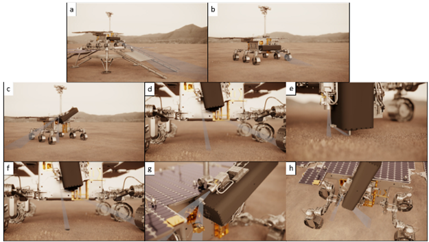
Figure 1: CLUPI science operational configurations. (a) On the platform, (b) geological environment survey, (c) Close-up outcrops observation, (d) drilling area observation, (e) drilling operation observation, (f) Drill hole and fines observation, (g) drilled core sample observation and (h) calibration: calibration target imaging. Images credit: ESA/SEI-TJ
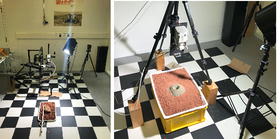
Figure 2: SEI CLUPI Science Operations Laboratory based in Microcity Neuchatel. Simulations using a CLUPI flight model representative. Images Credit: Space Exploration Institute (SEI)
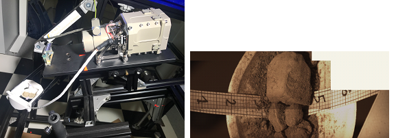
Figure 3: Left: CLUPI on the drill/rover simulator, sample observation configuration. Right: CLUPI output data, mosaic of three images. Images Credit: Space Exploration Institute (SEI). CLUPI Science Operations Laboratory based in Microcity Neuchatel. Simulations using a CLUPI flight model representative
How to cite: Josset, J.-L. and the CLUPI Team: CLUPI, Close-UP Imager on the ExoMars rover mission, Status and Science Operations Preparations/Simulations First Results, Europlanet Science Congress 2022, Granada, Spain, 18–23 Sep 2022, EPSC2022-1256, https://doi.org/10.5194/epsc2022-1256, 2022.
The WISDOM (Water Ice Subsurface Deposits On Mars) ground penetrating radar (GPR) (2)(3) has been specifically designed for the ExoMars (ESA/ROSCOSMOS) Rosalind Franklin rover to investigate the first meters below the surface of Oxia Planum in order to understand the geological context of the landing site and to provide guidance for sample collection by the drill.
The detection of clear buried interfaces or resolvable large reflecting structures might be the most rewarding features a GPR can reveal. Nevertheless, the shallow subsurface of some locations in Oxia Planum may be such as WISDOM radargrams would be difficult to interpret because of the lack of clearly identifiable structures. In particular, this will be the case if the subsurface consists in a heteregenous medium including a large density of scattering structures of dimension commensurate with WISDOM wavelengths of operation. Such scattering structures could be indicative of local changes in porosity or composition ; their characterisation is of interest as it provides information about the geological history and processes in the investigated area. This work proposes and tests a method to statistically estimate the typical size and, possibly shape, of buried scatterers and to retrieve their permittivity contrast with the surrounding material from WISDOM radargrams.
- WISDOM, GPR of the ExoMars mission
The WISDOM instrument is a step-frequency radar operating in a broad frequency bandwidth (0.5-3 GHz) corresponding to wavelength values ranging from 5 cm to 27 cm (for a relative permittivity value of 5), that ensures a vertical resolution better than 3 cm in the subsurface (1). WISDOM is also a polarimetric GPR. Thanks to its antenna system, it can acquire data in four polarization configurations (6) which allows an in-depth analysis of the received echoes for a better characterization of the shape and orientation of any buried reflector. These characteristics make WISDOM an instrument very well suited to the quantitative analysis of small-scale heterogeneities in the subsurface.
- Method
For this study, we have conducted numerical simulations with the code TEMSI-FD (4), which solves Maxwell equation using the Finite-Difference Time-Domain (FDTD) method. TEMSI-FD can simulate the propagation of WISDOM electromagnetic waves in realistic environments.
For the purpose of our study, we have considered subsurfaces embedding heterogeneities of fractal properties. These latters were generated by the diamond-square splitting technique implemented in the TEMSI-FD code. The resulting medium is characterized by 3 parameters : its mean relative permittivity mean, the standard deviation of its permittivity and the typical size of the heterogeneities L.
For a given set of these parameters, a number of subsurface volumes were generated in order to be able to perform meaningful statistical averages. Fig. 1 shows two examples of modeled subsurfaces with different L values and somewhat similar distributions of permittivity (right).

TEMSI-FD is used to simulate realistic WISDOM data for the study. The antennas and the transmitted signal are accurately modelled in order to reproduce as reliably as possible WISDOM operations over heterogenous media such as the ones displayed in Fig. 1. The orientation of the transmitting and receiving antennas can be changed to simulate the different polarimetric configurations. For one location of the radar, a single sounding provides the received amplitude as a function of the two-ways propagation time (Fig. 2). The mean of the signal envelope (red curve on Fig. 2) is computed to quantify volume scattering by heterogeneities (not considering the surface echo). Combining several soundings acquired at different radar location along a profile produces a radargram (Fig 3).

- Results and preliminary analysis
Fig 3 shows that volume scattering mostly occurs for L values ranging between 1.5 and 4.5 cm, with a maximum around 2.5 cm. Beyond 4.5 cm, no volume scattering is noticeable because the fractal heterogeneities can be regarded as individual reflectors at WISDOM wavelengths.

The broad frequency bandwidth of WISDOM allows to study the scattering process by sub-frequency band to estimate the typical size of the structures. The whole frequency domain is analyzed using 30 sliding sub-bands of 400 MHz width (to keep a sufficient temporal resolution), each being characterized by a mean wavelength λ = c / √εmean fmean where fmean is the mean frequency for the sub-band and c the celerity of light in vacuum.
Fig 4 synthetizes the results obtained for L values ranging from 1.5 to 4.5 cm; the error bars correspond to the standard deviation computed over 60 soundings. The results clearly show a maximum of scattering intensity for a wavelength λ ≈ 3.5 L regardless the value of L. This implies that, in principle, WISDOM data can be used to determine the size of heterogeneities within 1.7 cm and 10 cm in a porous subsurface (ε = 3) and within 1.0 cm and 5.7 cm in a compacted one (permittivity around 8). During the presentation, we will further discuss the validation and the implications of such a method of analysis which will be applied to terrestrial data acquired in a Martian analog, namely the Atacama desert (5). We highlight that the present work and proposed method can be readily adapted to other GPR operating from a planetary surface.

- Références :
(1) Oudart N. et al., PSS, Elsevier, 2021, pp.105173
(2) Ciarletti V. et al., Proceedings of the IEEE, 2011, 99 (5), pp.824-836.
(3) Ciarletti V. et al., Astrobiology, 2017, 17 (6-7), pp.565 - 584.
(4) Ciarletti V. et al., Monthly Notices of the Royal Astronomical Society, Volume 469, 2017, Pages S805–S817
(5) Dorizon S. et al., PSS, Elsevier, 2014, Vienna, Austria. pp.16078
(6) Plettemeier P. et al. 2009 IEEE Radar Conference, Pasadena, United States. pp.642-647
How to cite: Brighi, É., Ciarletti, V., Le Gall, A., De Lamberterie, F., Herve, Y., and Oudart, N.: Identifying heterogeneity sizes in the subsurface with WISDOM, the GPR of the ExoMars mission, Europlanet Science Congress 2022, Granada, Spain, 18–23 Sep 2022, EPSC2022-55, https://doi.org/10.5194/epsc2022-55, 2022.
Orals: Fri, 23 Sep, 10:00–13:30 | Room Manuel de Falla
Aqueous alteration minerals are high-value scientific targets and potential resources for future exploration. In particular, they are key drivers in the selection of contemporary and upcoming landing sites at Mars. Here we report on the “MOCAAS” (Mars Orbital Catalog of Aqueous Alteration Signatures) project, a 10-year endeavor which built a comprehensive high-resolution repository of aqueous minerals on Mars. Our project goals include: 1) providing a statistically meaningful global approach to aqueous minerals, 2) providing regional mineralogical context to better understand specific sites of interest, 3) identifying new high-science merit aqueous alteration mineral deposits, including as prospective landing sites, 4) providing groundwork for upcoming quantification work on the global inventory of volatiles sequestered in such minerals. A corollary are identifying sites which abundant aqueous alteration minerals provide ISRU opportunities for future human exploration.
We will present the first global-scale analyses of our detection sample, our benchmark of the methodology on rover landing sites, and discuss limitations, biases and perspectives.
We processed a large fraction of the OMEGA/Mars Express and CRISM/MRO datasets [Bibring+04; Murchie+07] which both allow retrieval of Mars surface reflectance in the [1.1-2.65] µm range used in this study. Their processing is described in [Carter+22] and yields aqueous alteration mineral detection (AMD) all over Mars. An AMD is a cluster of (nearly) contiguous pixels which we ascertained to contain similar spectral rationale for one or several aqueous minerals, to the sensibility limit of orbital near-infrared spectroscopy and observation spatial sampling. We combine several approaches that are systematic and semi-automatic as well as more refined manual investigations of individual observations from OMEGA and CRISM. Only confirmed AMDs are retained in the end which spectral content has been visually validated. We then further classify AMDs into 5 spectral-mineral classes: 1) Fe/Mg phyllosilicate clay, 2) Hydrous aluminosilicates and hydrated silica, 3) Poly/Semi-hydrated sulfate salts, 4) Mono-hydrated sulfate salts, and 5) Carbonates. These classes account for degeneracies in the diagnostic spectral features which cannot always be uniquely attributed to a given alteration mineral.
Excluding polar latitudes, a large fraction of the Mars surface mineralogy has been surveyed at a sampling down to 200 m/pixel (>62% of the surface) using semi-automatic algorithms, and its near entirety at kilometric resolution. Candidate AMDs were then further investigated in detail at all resolutions. The total fraction of AMDs reported at Mars is ~1%, yet this fraction includes many terrains that exhibit surface dust, poor observational conditions, and are younger than the late Hesperian. Figure 1 provides the global distribution color-coding for spectral mineral classes which is seen to strongly correlate with the oldest, dust-poor terrains of Mars.
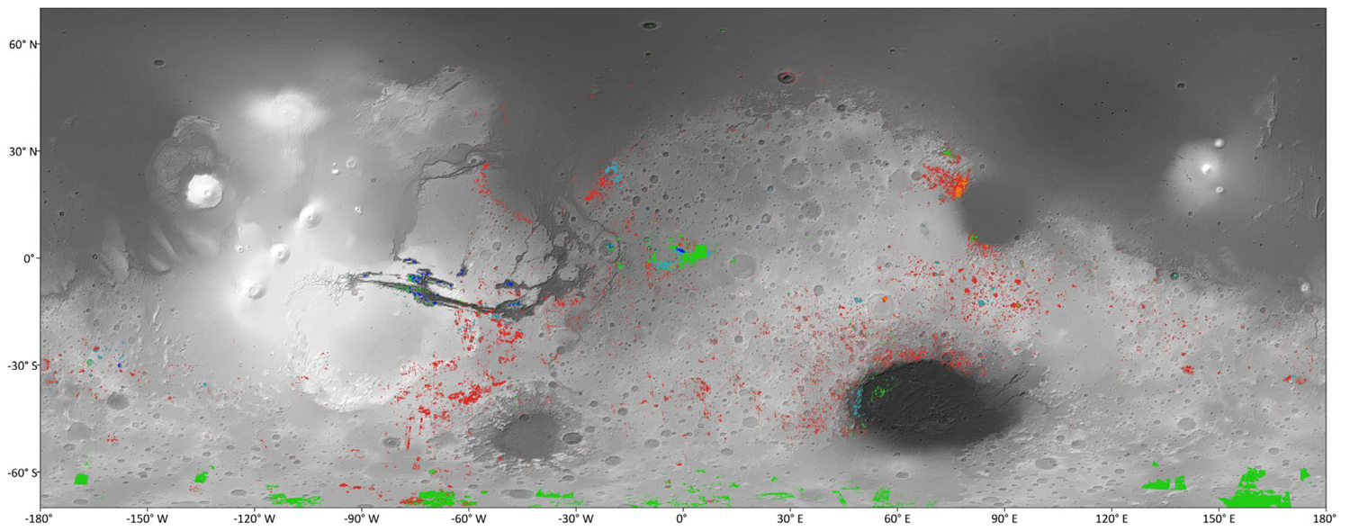
Figure 1: Distribution of aqueous alteration mineral detections based on the OMEGA and CRISM datasets. Each color codes for the spectral mineral classes (Red: Fe/Mg phyllosilicates; Green-blue: sulfate salts; Orange: carbonates; Cyan: aluminosilicates or hydrated silica). Each color pixel here indicates that alteration minerals are present within a 4x4km² area.
Preliminary analyses of the global distribution of aqueous alteration minerals will be presented, investigating distribution as a function of latitude, altitude, unit type and unit age. An example histogram of the distribution of aqueous minerals as a function of unit age is shown in Figure 2. In particular, we report the much more widespread occurrence of several types of aqueous minerals throughout the Noachian highlands of Mars compared to what was previously known.
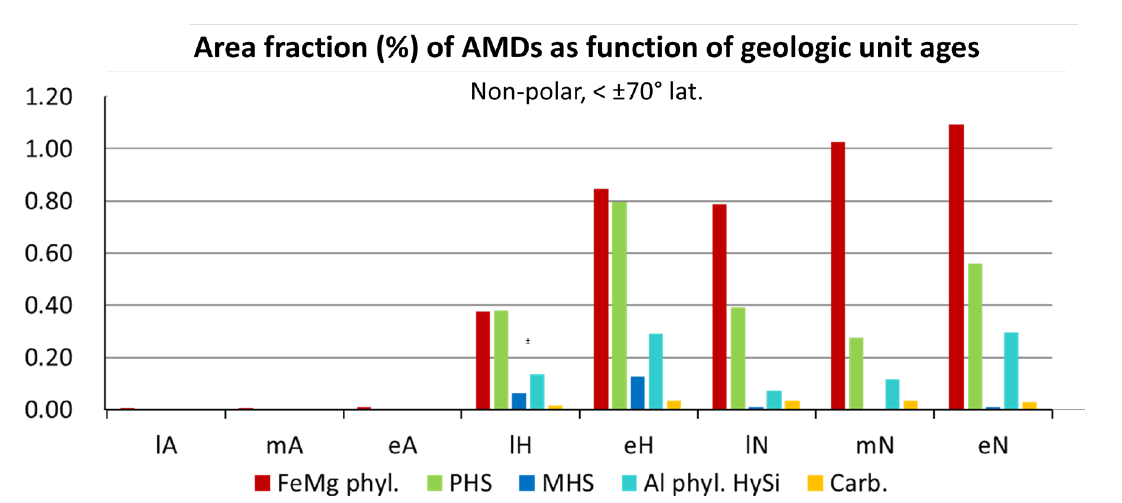
Figure 2: preliminary statistics on the distribution of alteration minerals, as a function of their unit-age from [Tanaka+14].
Our detection capability is then benchmarked by implementing the same mapping procedure but applied to well-studied candidate or current landing sites for rover missions: at Gale crater, Jezero Crater, Mawrth Vallis plateaus and Oxia Planum. For these, we generate local high resolution maps, for which an example is given at Jezero crater below.
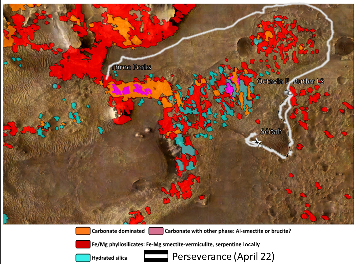
Figure 3: High resolution aqueous alteration mineral mapping of the surroundings of Mars 2020 in Jezero crater.
We will discuss perspectives for both global analyses of aqueous minerals made possible by this catalogue (e.g. [Riu+22]), as well as regarding future studies of newly identified sites of interest for which we will present a sample.
In the near-term, the MOCAAS catalogue of aqueous alteration minerals will be made available on the PSUP portal (psup.ias.u-psud.fr) as well as through a dedicated web portal.
References: [Bibring+04] J.-P. Bibring et al., ESA Spec. Pub, 2004, https://ui.adsabs.harvard.edu/abs/2004ESASP1240...37B; [Murchie+07] S. Murchie et al., JGR, 2007, 10.1029/2006JE002682 ; [Carter+22] J. Carter et al., Icarus, under revision ; [Tanaka+14] K. Tanaka et al., 2014, http://pubs.er.usgs.gov/publication/sim3292 ; [Riu+22] L. Riu et al., this conference.
How to cite: Carter, J., Riu, L., Poulet, F., Bibring, J.-P., Langevin, Y., and Gondet, B.: Global distribution of Mars aqueous alteration minerals from orbit: the MOCAAS project, Europlanet Science Congress 2022, Granada, Spain, 18–23 Sep 2022, EPSC2022-185, https://doi.org/10.5194/epsc2022-185, 2022.
In the past decades, numerous hydrated silicates have been detected at the surface of Mars from orbital and in situ characterization. Understanding the hydrated mineralogy of Mars constitutes an important goal to retrace its water history and to evaluate its resource assets in terms of water budget. In addition to providing information on the past aqueous subsurface and surface environments, the aqueous alteration minerals (e.g., secondary phases) have a major exobiological potential and are prospective resources for human exploration and in situ resource utilization (ISRU, [1]). As such they are key drivers in the selection of current and upcoming landing sites for robotic and human missions to Mars. With a more global and quantitative view of the altered mineralogy (as presented in [2]) the modal composition can be accessed and the water content stored in hydrated silicates present at/near the surface can be evaluated. By quantifying the content of each minerals at the hydrated sites, the estimation of the water content stored at the surface within these minerals is then quite straightforward. The global mineralogical maps of [2] were used. They were derived using the full dataset of the OMEGA instrument, where the global abundances of 11 hydrated silicates can be found: Fe-Mg dominated smectite, Al-smectite, AlSiOH, Opal, Mg-carbonates, Chlorite, Fe/Mg-Micas, Serpentine and Fe-hydroxide. A set of non-hydrated minerals is also included in the mixture but is not used to derive the water content as they do not contain OH or H2O. To evaluate the water content of each individual end-member, the potential chemical formula of each end-member was first evaluated and then the weight percent of H2O or OH in the formula was estimated. This methodology is based on [3]. Thus, for each end-member several estimations of the water content are computed. They depend on the selected formula (the exact formula being unknown at Mars) and on the estimated hydration state (being also unknown) of each mineral. Then, the abundance of each end-member in water content is evaluated by multiplying their abundance with their individual water weight percent and by summing at each location (i.e., each pixel of the map) all the resulting water contributions. The resulting global map of water content at a resolution of ~ 1 km per pixel at the equator is shown on Figure 1.
The average content of water, based on the content stored in hydrated silicates, is estimated to be slightly above 5 wt%, with some rare occurrences > 20 wt% (examples of such occurrences are shown on Figure 1). These values are in good agreement with previous orbital estimations of the water content at Mars based on other estimations techniques ([4],[5]) that predicted 2-7 wt% on average at the surface.
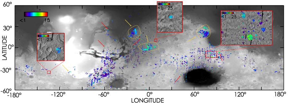
Figure 1 - Global map of water content (wt%) at Mars, as stored in hydrated silicates. The red arrows point at location of 100s km2 were the water content at the surface is consistently > 10 wt%. Three zoomed maps are shown to illustrate specific settings that provide a high-water content at the surface. The orange arrows and circles highlight the large deposits of Marwth Vallis, Nili Fossae and Meridiani Planum.
The ongoing studies now aim at a detailed analysis of the water distribution in order to look for new regions with high past aquability (stable liquid water) potential and/or exobiological potential, if such locations exist. The map will be studied locally (see Figure 1) in combination with high resolution images in order to correlate the high-water content with their context and highlight new regions of interest. Incorporation of ground-truth knowledge from Perserverance at Jezero crater is foreseen so as to refine the mineral endmembers, and make abundance comparisons on the larger mineral units which will be sampled.
References
[1] Abbud-Madrid, A., et al. (2016). Mars Water In-Situ Resource Utilization (ISRU) Planning (M-WIP) Study 90.
[2] Riu, et al. (2022). The M3 project: 3 – Global abundance distribution of hydrated silicates at Mars. Icarus 374, 114809. https://doi.org/10.1016/j.icarus.2021.114809
[3] Wernicke, L.J. & Jakosky, B.M. (2021). Martian Hydrated Minerals: A Significant Water Sink. J. Geophys. Res. Planets 126. https://doi.org/10.1029/2019JE006351
[4] Audouard, J., et al. (2014). Water in the Martian regolith from OMEGA/Mars Express: Mars 3 µm absorption and water mobility. J. Geophys. Res. Planets 119, 1969–1989. https://doi.org/10.1002/2014JE004649
[5] Milliken, R.E. et al. (2007). Hydration state of the Martian surface as seen by Mars Express OMEGA: 2. H 2 O content of the surface: HYDRATION STATE OF THE MARTIAN SURFACE. J. Geophys. Res. Planets 112. https://doi.org/10.1029/2006JE002853
How to cite: Riu, L., Carter, J., and Poulet, F.: Estimation of H2O content (in wt%) stored in hydrated silicates at Mars and implications for In Situ Resource Utilization (ISRU), Europlanet Science Congress 2022, Granada, Spain, 18–23 Sep 2022, EPSC2022-132, https://doi.org/10.5194/epsc2022-132, 2022.
- Introduction
In order to study unaltered rocks, Mars rovers are equipped with abrasive and/or drilling devices. NASA’s Spirit and Opportunity rovers were equipped with a Rock Abrasion Tool to remove the first mm of altered material [1]. NASA’s Curiosity and Perseverance and ESA’s Rosalind Franklin ExoMars rovers are equipped with drilling device to collect samples for in situ analysis and, for Perseverance, in preparation for a future Mars Sample Return mission [2-4]. During these drilling phases, a pile of rock powder, of varying size depending on the drilling depth, forms at the surface.
The objective of the ExoMars mission will be to search for past or extant biosignatures for which drill-cores will be collected from up to 2 meters deep; the depth at which organic matter is preserved from degrading UV and particle irradiation. The drill has a diameter of 3 cm. The cone of powder at the surface could thus represent more than 1.5 dm3, a relatively large quantity of material which will not be analysed by the instruments inside the rover but which could be observed by the CLUPI and PanCam cameras [4-6].
Powder can be considered as a textureless material when the grain size is lower than the spatial resolution of the photograph, which is the case for rocks drilled on Mars as observed by MSL [2]. Colour is then the only measurable data; however, this apparent colour is totally dependent on ambient light and on the camera itself. In order to solve this problem, we have developed a new method called CaliPhoto, for which a reference plate is added to the camera's field of view and then image processing is used to compensate for camera characteristics and lighting conditions [7,8]. The images thus obtained can then be compared with each other or with a reference database. Here, we used a series of analogue rocks to demonstrate the ability of the method to identify volcanic rock powders on Mars.
- Materials and methods
The majority of rocks on the surface of Mars are volcanic [9,10] thus, for this study, 23 relevant samples were selected from the Massif Central, in France, in order to cover a large range of volcanic rock types, as designated in the compositional TAS diagram (Total Alkali Silica). The samples were then crushed and each powder was placed in the centre of the CaliPhoto reference plate and photographed. The CaliPhoto image processing was then used to “calibrate” the photographs and a database was created (see Fig. 1).
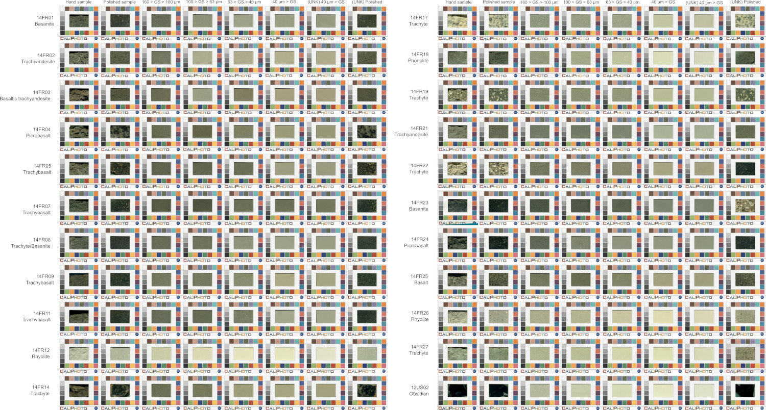
Figure 1: Images of the volcanic rock samples after CaliPhoto image processing.
- Results and discussion
Different tests were carried out [8]. First, each sample was photographed twice in different lighting conditions, the first image was imported into the database and the second was used to test the identification procedure. For 50% of powders, the identification is exact, i.e., the studied powder corresponds to the highest matching identification from the database, in 77% of cases, the studied powder is in the top two matches, and in 95% of cases, it is in the top three. Moreover, when the studied powder is not in the first position, the best match occurs for a rock of similar or close composition.
The analogue rock ESA-01-E (picrobasalt), chosen by ESA for its physical and chemical similarities to known Martian rocks, was then used to test the ability of the method to evaluate the composition of a powder that is not in the database. The method successfully identified the sample as a picrobasalt.
The rocks were crushed at 4 different grain sizes in order to evaluate the effect of grain size distribution on the method. Indeed, the apparent luminosity of powder is known to increase with decreasing grain size. For 32% of the powders the identification is exact, i.e., the studied powder corresponds to the highest matching value. Moreover, for 91% of cases, a rock with a similar or adjacent composition as defined by the TAS diagram is in the top three matches, even when the powder is not in the database.
Finally, by coupling hand sample and powder colour vectors, the identification is exact for 68% of rocks and the studied sample is in the top three matches in 100% of cases. Moreover, when the studied sample is only in the second or third position, the difference with the best match is always lower than 1%.
- Conclusion and perspectives
The CaliPhoto method could be very useful on Mars to help identify rocks during drilling without adding any new instrumentation except a specific colour plate that could be positioned near the powders. Unfortunately, Mars rovers are not equipped with such a plate. Thus we proposed to use the calibration targets present on the rovers to calibrate the colour of the martian floor before drilling then to use it as reference for the CaliPhoto method. The first tests were relatively conclusive.
Finally, with the postponement of the mission, the CaliPhoto colour plate could constitute a good complement to the ExoMars rover.
Acknowledgements
We acknowledge the Maison du parc national des volcans d’Auvergne for permission to sample. We thank CNRS, CNES and SATT Grand Centre for funding.
References
[1] Gorevan S. P. et al. (2003) J.-Geophys.-Res. 108.
[2] Abbey W. et al. (2019) Icarus 319, 1–13.
[3] Farley K. A. et al. (2020) Space Sci. Rev. 216, 142.
[4] Vago J. L. et al. (2017) Astrobiology 17:6-7, 471–510.
[5] Josset J.-L. et al. (2017) Astrobiology 17:6-7, 595–611.
[6] Coates A. J. et al. (2017) Astrobiology 17:6-7, 511–541.
[7] Foucher F. et al. (2019) Inventions 4, 67.
[8] Foucher F. et al. (2022) Icarus 375, 114848.
[9] McSween H.Y. et al. (2009) Science 324, 736, 2009.
[10] Bost N. et al. (2013) Planet. Sp. Sci. 82-83, 113-127.
How to cite: Foucher, F., Bost, N., Guimbretière, G., Hickman-Lewis, K., Courtois, A., Luengo, L., Marceau, E., Martin, P., and Westall, F.: CaliPhoto: a powerful method to identify rock powders on Mars, Europlanet Science Congress 2022, Granada, Spain, 18–23 Sep 2022, EPSC2022-138, https://doi.org/10.5194/epsc2022-138, 2022.
Introduction: Successful exploration of Mars could benefit from a detailed knowledge of mineralogy of Martian surface materials [1]. One of the most explicit studies of minerals on Mars, would be done on Martian meteorites. Dar al Gani 476 is one of the most mafic basaltic shergottites found so far [2] which was found in the Saharan desert in Libya in 1998 from the Dar al Gani region. The volume of the sample is 4.15 × 8.58 mm, the thickness is 0.88 mm and it weights 0.1511 gr. It is an igneous rock rich in olivine and pyroxene, with some shock metamorphosed minerals and glass. In this work, to achieve high accuracy on the mineral identification of the igneous rock, we applied a combination of FTIR microspectroscopy and Raman spectroscopy.
Methods: The Raman spectra were obtained from an inVia Renishaw Raman imaging spectrometer with a high spectral (1cm-1) and spatial resolution. The excitation wavelengths of 532 nm laser line was used for this study. Scanning of a big area of the sample covers the areas of 837 × 534 µm, using 50× long working distance objective, 5s exposure time and 10% of the laser power (4.59mW). MicroFTIR mapping was done by the Thermo Scientific nicolet Infrared Microscope. Back-scattered electron images (BSE) were taken with Hitachi S-3400N Scanning electron microscopy with energy dispersive spectrometers (EDS) (EMU, Hong Kong University).
Results and Discussion: The BSE image of DaG 476 illustrates its porphyritic texture (Figure 1). As a most mafic basaltic shergottite, it contains olivine and pyroxene with a high Mg content. EDX elemental maps reveal the presence of Si, Al, Ca, Mg, Fe, and P and other elements, including Na, S, Cr and C [3] (Figure 2).
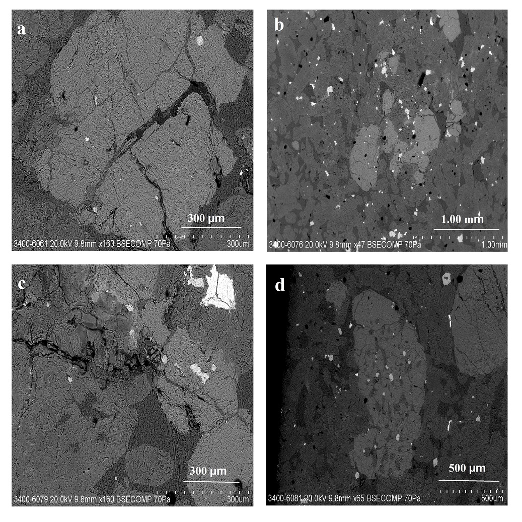
Figure 1. BSE image of DaG 476. (a) large light-gray grains are olivine, (b) white dots are representatives of silicon, (c) white phases are Fe-oxides and sulfide, (d) large pyroxene grains with dark cores, black areas are feldspathic glass.
Raman mapping and distribution of minerals has been shown in Figure 3. The presence of anhydrous silicates such as olivine and augite has been observed. Augite and enstatite show Raman peaks at 231, 323, 388,664, 675, 1006 and 1013 cm−1 (Table 1). The range and distribution of pyroxene compositions indicate that the rock did not cool and crystallize slowly [4]. This broad range of pyroxene composition is consistent with chemical zoning preserved during rapid crystallization and supports a basaltic texture.The presence of the volcanic glass, suggest that rock had been shocked and cooled rapidly with mineral crystal growth. Feldspar melting glass consists mainly of glass (> 97%) and rich in the lighter elements such as Si, O, Al, Na and as an evidence of past volcanic activity, its plagioclase feldspar was converted to a volcanic glass [5].
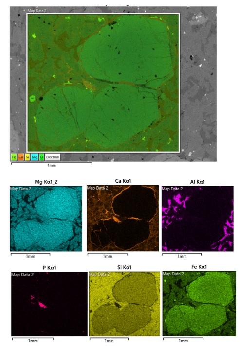
Figure 2. EDX elemental map from of the DaG 476 sample.
Table 1. Specific Raman peaks of DaG 476 Martian meteorite sample and the minerals designation.
|
Mineral |
Raman peaks/cm-1 |
|
Raman Catalogue (https://rruff.info) | |||||||
|
Olivine |
816 |
848 |
822 |
851 |
||||||
|
Augite |
323 |
388 |
664 |
1013 |
328 |
395 |
665 |
1011 |
||
|
Chromite |
281 |
322 |
670 |
677 |
1004 |
1086 |
337 |
680 |
684 |
1006 |
|
Glass |
483 |
961 |
989 |
1007 |
484 |
960 |
998 |
|||
|
Enstataite |
231 |
655 |
675 |
1006 |
238 |
344 |
664 |
686 |
1012 |
Glassy materials have weaker Raman scattering than crystalline minerals. Although glassy materials often dominate the spectrum, the Raman peaks of glass can be easily masked by the peaks of the crystalline phases when they are sampled together. The rock might be sufficiently shocked and its plagioclase might have bene destroyed (Figure 3).
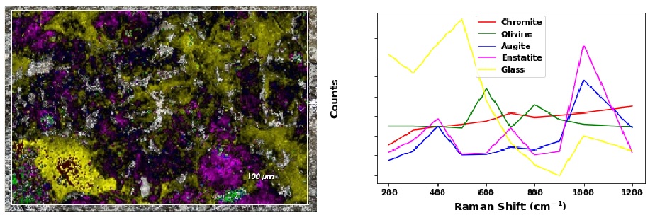
Figure 3. Compositional map of the DaG 476 and Raman spectra of minerals
Figure 4 shows the presence of carbonates in the sample which probably formed on earth once the meteorite landed. It’s confirmed as terresterian carbonate due to having a noticeable effect on the bulk oxygen isotopic composition [6]. It is concluded in previous research that carbonate component of DaG 476 is associated with impact-melt pockets [6]. In the porphyritic texture of the meteorite, a fine grained ground mass of clinopyroxene is surround by olivine. The pyroxene consists primarily of pigeonite and augite, although enstatite has been observed by Raman spectrsocopy [7].
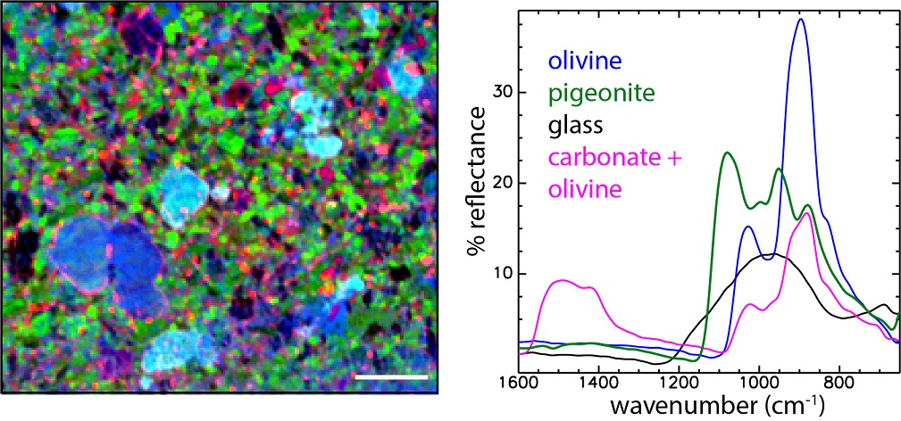
Figure 4. Distribution of minerals in the FTIR image of Dag 476 and IR spectra of minerals.
Conclusions: This work confirms the potential value of Raman spectroscopy and FTIR microspectroscopy for mineral analysis of different types of meteorites and returned samples. Peak positions and spectral patterns have lead us to identify the minerals and their distribution in DaG 476 sample. DaG 476 has a fine-grained groundmass consisting of pyroxene and the fine-grained amorphous silicate material found in veins and pockets, isolated olivine and single chromite grains occur in the groundmass. The spectra of the volcanic glass has been detected in the rock which may have been formed when lava of a volcano cooled rapidly, i.e. the DaG 476 may be separated from a part of the surface where lava was flooded in ancient times. Combination of Raman spectroscopy and FTIR microspectroscopy provide a capability to estimate the carbonate minerals and silicates in meteorites and planetary analogue samples.
References: [1] Wang, A., et al. (2003) Journal of Geophysical Research: Planets, 108(E1). [2] Zipfel, J., et al. (2000). Meteoritics & Planetary Science, 35(1), 95-106. [3] Wadhwa, M., et al. (2001). Meteoritics & Planetary Science, 36(2), 195-208. [4] Borg, L. E. et al. (2003). Geochimica et Cosmochimica Acta, 67(18), 3519-3536. [5] Crozaz, G., & Wadhwa, M. (2001). Geochimica et Cosmochimica Acta, 65(6), 971-977. [6] Wright, I. P., et al. (1999). In Lunar and Planetary Science Conference (p. 1594). [7] Borg, L. E., et al. (2003). Geochimica et Cosmochimica Acta, 67(18), 3519-3536.
How to cite: Tanbakouei, S., Michalski, J. R., and Wright, S. P.: Mineralogy of shergotite Dar al Gani 476 as an analogue of Martian surface, Europlanet Science Congress 2022, Granada, Spain, 18–23 Sep 2022, EPSC2022-947, https://doi.org/10.5194/epsc2022-947, 2022.
Introduction: The behavior and the rheology of mud during the emplacement of terrestrial sedimentary volcanism has been previously investigated (e.g., [1,2]). In contrast, this is not the case for Mars nor for other planetary bodies within the Solar System for which sedimentary volcanism has been proposed [e.g., 3]. The propagation behavior of low viscosity mud in a low-pressure chamber that partly simulated the surface environment of Mars was experimentally studied for the first time by [4,5]. Their work revealed that low viscosity mud flows could propagate over cold (<273 K) and warm (>273 K) surfaces at martian atmospheric pressure, however, the mechanism of such propagation is different to that observed on Earth. On Mars, mud propagating over cold surfaces should rapidly freeze due to evaporative cooling [6] forming an icy-crust leading to propagation in a similar manner to pahoehoe lava flows on Earth [4]. In contrast, mud propagating over a warm surface boils and levitates above the surface. The viscosity of ascending mud varies depending on its water content, and the behavior of high viscosity mud under martian atmospheric pressure remains unexplored.
Experimental setup: We used the Mars Simulation Chamber at the Open University (UK) into which we inserted a 0.9 × 0.4 m plastic box filled with a ~10 cm thick layer of natural sand (ø ~200 µm) mixed with water to limit the infiltration of mud into the sand and to better maintain the temperature below 0°C. Inside was placed a container to accommodate 600 ml of mud (Fig. 1). The infilled box was cooled to a temperature of ~-20°C. The temperature of the mud when inserted into the container was 1-3°C and 20-22°C respectively. Two different viscosities were tested – the first mix contained 50 wt% clay (a bentonite composed of 76% montmorillonite, 23% illite and 1% kaolinite) and water (1:1 mix). The other was prepared by mixing 75 wt% clay with 25 wt% water (3:1). The pressure was gradually reduced from 1 bar to 6 mbar within a timeframe of minutes (rapid) or in >hour (slow). Each experimental run was triplicated to confirm reproducibility.
Observations: With the 1:1 mixture, once the atmospheric pressure was reduced, the mud started to boil (Figure 2). In the case of mud at room temperature and a rapid pressure drop, significant boiling caused an ejection of muddy droplets from the container into the surroundings. Such behavior was not observed for other experiments and mud was extruded due to the volumetric increase. Once the pressure dropped below 7 mbar, freezing occurred leading to the formation of an icy-muddy crust. Once this crust covered the entire mud surface, additional boiling and volumetric increase was limited. However, when the crust broke up, gasses were capable to escape and the deflation was observed.
For the 3:1 mixture vigorous boiling was not observed during the pressure drop. Instead, as the pressure decreased, the mud volume increased and sets of cracks developed on the surface. Regardless of the tested parameters, the volumetric increase was observed during all experiments as bubbles within the mud developed and increased their volume. In the case of 1:1 and 3:1 mixture the mud inflation reached up to ~15% and ~28% respectively (the observed volumetric changes were quantified by semi-manual processing of selected images using the PIV [Particle Image Velocimetry] and photogrammetry methods). In addition, we also observed a partial collapse of the newly formed foamy edifice as the gas trapped inside the mud escaped. This inflation and deflation of the mud often repeated and the magnitude of volumetric change leads to different morphologies (Figure 3).
Discussion and conclusion: The volumetric increase is caused by the formation of small water vapor bubbles which are trapped within the mud (Figure 4). The buoyancy of the bubbles is not sufficient to overcome the drag force within the viscous material and rise to the surface. Hence, these bubbles remain trapped and gradually grow up to centimeter scale sizes. During their growth they push the mud out of the container resulting in horizontal and vertical inflation of the mud surface over cm- scales (e.g., see outlines in Figure 2). This behavior is not observed at terrestrial mud flows. Our experimental approach hence shows that viscous mud exposed to reduced atmospheric pressure behaves differently when compared to conditions on Earth.
Acknowledgments: The access to the Large Mars Chamber at the Open University was provided by Europlanet 2024 RI which has received funding from the European Union's Horizon 2020 research and innovation program under grant agreement No 871149.
References: [1] O’Brien and Julien (1988), Journal of Hydraulic Engineering 114 [2] Laigle and Coussot (1997), J. Hydraul. Eng., 123 [3] Ruesch et al. (2019) Nature Geoscience 12 [4] Brož et al. (2020), Nature Geoscience [5] Brož et al. (2020), EPSL 545 [6] Bargery et al. (2010), Icarus 210(1).
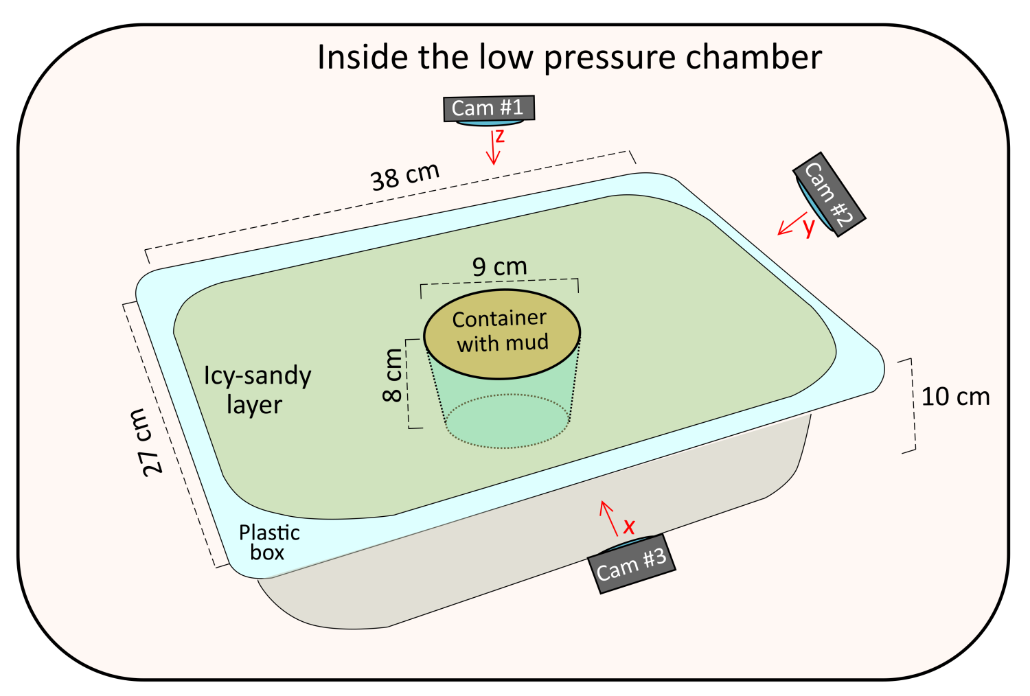
Fig. 1: Experimental setup.
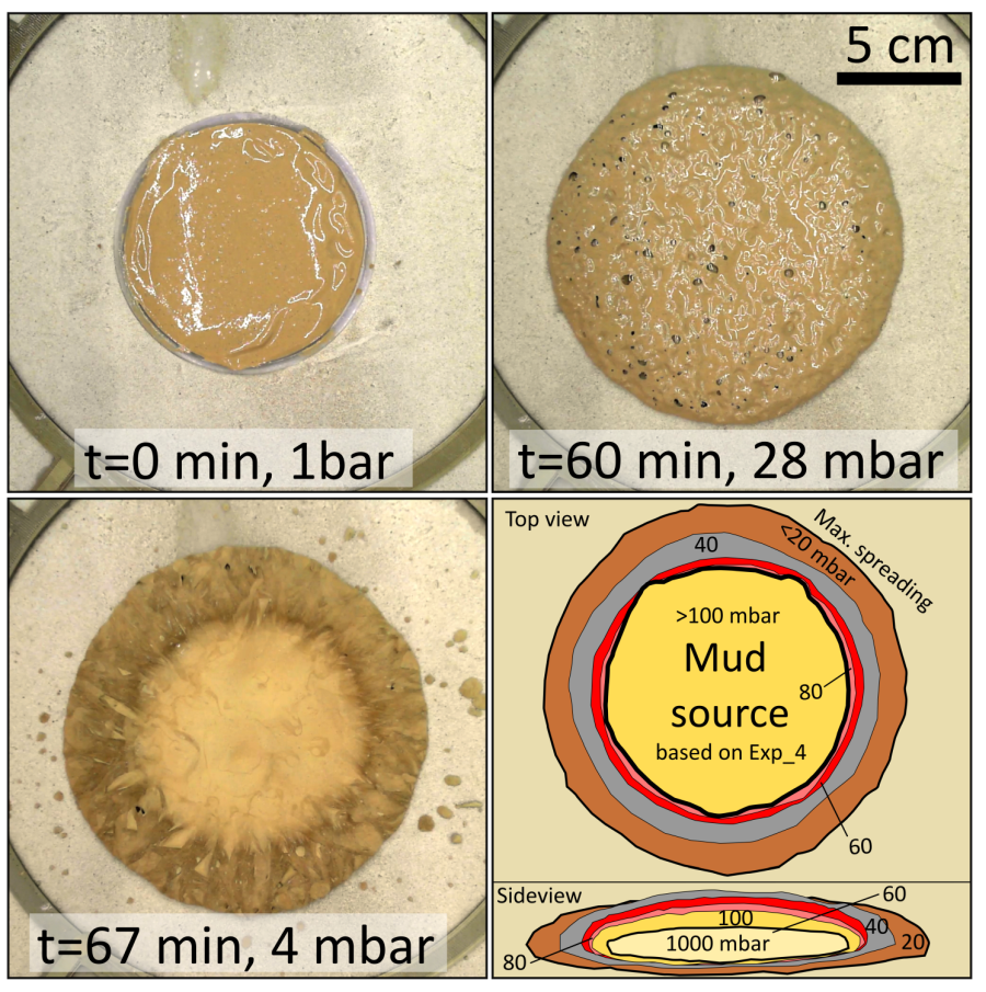
Figure 2: A sequence of images capturing the volumetric change of 1:1 mud (T=1°C) depending on the pressure value. The simplified sketch shows the extent of such changes indicated with different colors.
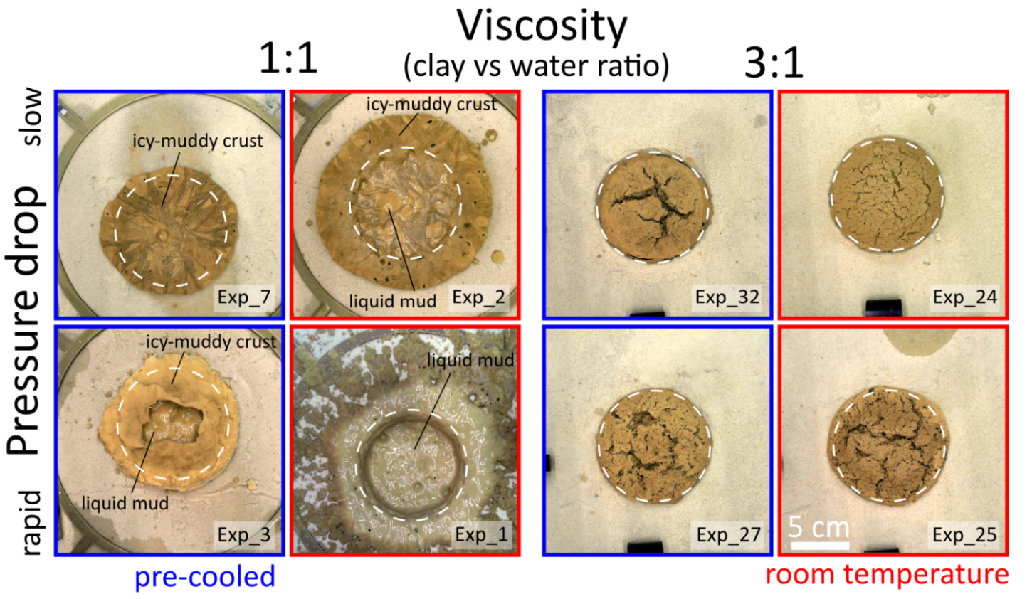
Figure 3: Examples of morphologies resulting from inflation of the mud induced by low pressure conditions. The blue and red boxes mark different temperatures of the mud. Morphologies of 3:1 mud are relatively uniform, in contrast a wider variety exists for less viscous 1:1 mud. The white dashed lines mark the position of the 9 cm large container.
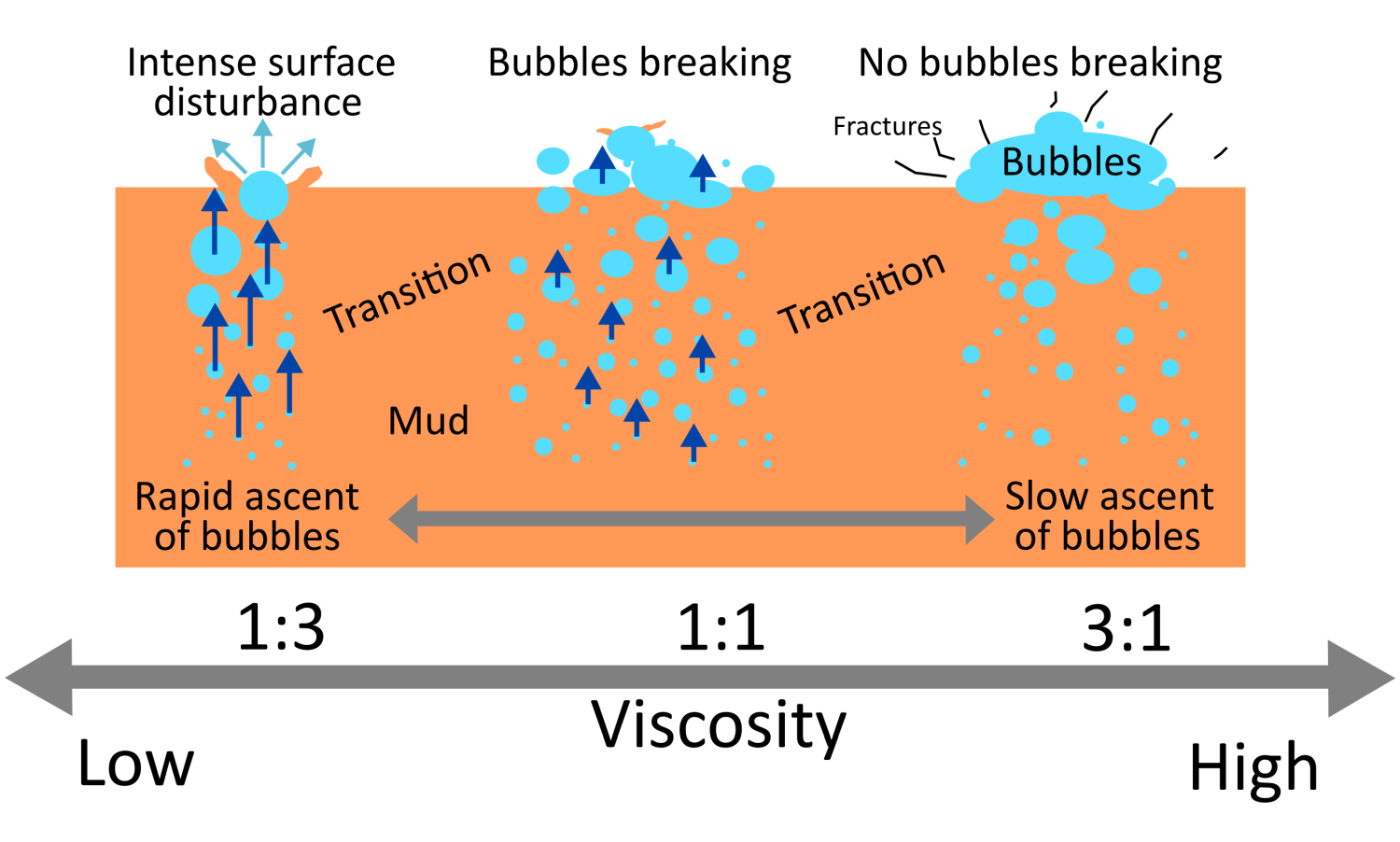 Figure 4: Simplified concept of mud inflation due to the pressure drop. Behaviour of 1:3 mud based on work of [4].
How to cite: Brož, P., Kryza, O., Conway, S., Mazzini, A., Hauber, E., Sylvest, M., and Patel, M.: Volumetric changes of mud on Mars: Evidence from laboratory simulations, Europlanet Science Congress 2022, Granada, Spain, 18–23 Sep 2022, EPSC2022-548, https://doi.org/10.5194/epsc2022-548, 2022.
The High Resolution Imaging Science Experiment (HiRISE) on the Mars Reconnaissance Orbiter (MRO) routinely observes the surface of martian polar regions during seasonal observational campaigns. The images reveal a variety of seasonal features related to CO2 jet eruptions. The amount and quality of the data collected over 8 martian years provides abundant information on seasonal and inter-annual development of these transient surface features – fans and blotches – considered to be dust and sand deposits from the CO2 jet eruptions. Directions and sizes of the fan deposits showcase information about eruption physics as well as about the state of the martian atmosphere at the time of eruption.
To analyze the HiRISE dataset numerically we have created a citizen science project Planet Four (P4). Participants of P4 mark seasonal deposits in sub-frames of HiRISE images with provided tools that have specific geometry. Locations, directions, and sizes of the markings are stored in a database. We have created a pipeline that works with the database, removes mistaken markings, and reduces multiple markings of the same object to the statistically best marking per object. The result of the pipeline is a catalog of fan and blotch markings that provide direct information about wind directions and speeds in the locations observed. The fan directions shift considerably during spring which is indicative of the volatile nature of weather in the southern polar regions in spring as the polar vortex develops. We will present derived wind speeds and directions in multiple regions of interest (ROIs) in the southern polar regions.
We have run the Mars Regional Atmospheric Modeling System (MRAMS) at the same locations and portions of spring to compare its results to values derived from P4. The MRAMS model is generally consistent with P4 wind directions and speeds derived from P4 fan sizes. MRAMS winds are most consistent with the observed directions in early spring, while after approximately Ls = 200° the model tends to be a bit less consistent with the P4 observations. This can be explained in part by the relative proximity of the sublimating edge of the seasonal polar cap at these times, which tends to increase the wind direction variability.
MRAMS winds are calculated every 10 Mars-minutes for multiple complete martian days, providing an opportunity to determine the timing of jet eruptions. In some of the ROIs we observe a correlation of P4-determined winds with modeled winds at specific times of day. This indicates that CO2 jet eruptions happen during those specific times. The most probable time of jet eruptions determined from these correlations varies through spring. This is consistent with CO2 jet modeling that suggested that timing of jet eruptions is connected to the amount of available solar energy. In the early spring those CO2 jet models expect the eruptions to occur close to local noon or during the afternoon, while later in spring they are expected to shift to earlier hours of the day as the seasonal ice thins. Not all P4 ROIs exhibit this pattern when compared to the MRAMS simulations. Local wind patterns and the near-surface atmospheric environment (where eruptions happen) have to be examined in detail to understand and decouple the sporadic nature of CO2 jet eruptions from the dynamic atmospheric behavior modeled by MRAMS.
Conclusions: HiRISE and consequently P4 data created several new ways to investigate seasonal processes and atmospheric dynamics on Mars with the potential for quantitative analysis.
How to cite: Portyankina, G., Michaels, T., Schwamb, M. E., Aye, K.-M., and Hansen, C. J.: Studying polar CO2 jet eruptions and the state of the lower martian atmosphere with help from the Planet Four citizen science project, Europlanet Science Congress 2022, Granada, Spain, 18–23 Sep 2022, EPSC2022-750, https://doi.org/10.5194/epsc2022-750, 2022.
Introduction
Observations from OMEGA, the visible-near infrared hyperspectral imager onboard the Mars Express orbiter, highlighted spectral variability of the Martian high latitude surfaces [1]. In particular, the 1.9 µm and 3 µm band depths increase from 60° latitudes towards the poles [1, 2, 3], which suggests that hydrated minerals may participate in this spectral variability. [3] reported the detection of a deep and relatively narrow absorption band at 3 µm coupled with a shallow but significantly wider 4 µm feature in the northern high latitudes of Mars, with no significant counterpart in the south for now. Comparison with laboratory spectra suggest that these features may be associated with the presence of salts such as sulfates and/or perchlorates [3]. In the south polar region, several absorption features related to water-bearing minerals (e.g., sulfates, phyllosilicates) have been identified in the 1 – 2.6 µm spectral range [1, 4]. As a result, sulfate salts were mapped over large areas there, but their precise mineralogy and distribution is not constrained [4]. Moreover, the 1.9 µm band is significantly broader and shifts to slightly longer wavelengths in the south which seems to indicate a specific mineralogy, and/or a different hydration state from that of the north [1]. Here we present the preliminary results of a study about the combined evolution of the spectral features identified in the southern high latitudes.
Method
The OMEGA (Observatoire pour la Minéralogie, l’Eau, les Glaces, et l’Activité) instrument has been observing the surface of Mars since 2004 between 0.35 and 5.1 µm. Here, we selected observations acquired during southern spring and summer as high latitudes are covered by seasonal ice during winter. Our analyses focus on the detection and characterization of hydrated minerals, in particular sulfates, using several spectral criteria previously defined: the band depths at 1.9 µm [5], 2.1 µm [6] and 2.4 µm [3]; the narrow [3] and wide 3 µm band depths [2]. We have also developed a new estimator for the wide band depth observed around 2 µm in the south polar region [1]:

where is the average reflectance from the n spectels corresponding to wavelengths (µm). Since the 3 µm band is very sensitive to the presence of water ice at the surface or in the atmosphere [7], we remove pixels with a water ice absorption at 1.5 µm>1%. In order to prevent possible effects related to viewing geometry, we removed pixels with emergence and incidence angles respectively higher than 10° and 75°.
Preliminary results
The parameters exhibit a strong variability in the south polar region (Figure 1 and 3) which suggest possible variations of the hydration state and/or mineralogical composition of the surface. As already demonstrated, the 1.9 µm and the wide 3 µm band depths increase towards the pole (Figure 2 and 3). The intensity of the “narrow 3 µm band” criteria such as defined by [3] is significantly (two times) lower than in the north polar region. The wide band depth around 2 µm is higher than 3% in the whole area and increases up to 5% at 75°S. Beside this regional spectral variability, we can also notice localized area which may have a specific spectral pattern, e.g., near 58°S where the 3 µm band shape is modified in such a way that the wide band depth criteria is reduced while the narrow one increases; at the same time the 2.4 µm band is reduced while the wide 2 µm criteria increases (Figure 2 and 3). Although not following as clear a latitudinal trend, we find large areas of hydrated sulfate salt signatures through a combination of the 1.9 µm band and 2.4-2.5 µm spectral shoulder. These occur preferentially at high southern latitudes.
Perspectives
Preliminary results show a large range of diversity in the near-infrared between 1.4 and 2.6 µm but also around 3 µm (Figure 1). The band depths at 1.9 and 3 µm are strong indicators of the surface hydratation [2] and bands in the 1.9 - 2.1 and 2.4 µm ranges may be associated with sulfates [4, 8]. By using these band depths and additional spectral criteria, we plan to estimate the coverage and properties of hydrated minerals, in particular sulfates, in the south polar region, following previous studies by [1] and [4]. We also plan independent validation and further characterization of the mineralogy of some of these areas using CRISM high-resolution observations. This reappraisal of available spectral constraints compared with the geomorphological context will improve our understanding of the formation scenarios of the hydrated minerals, in particular sulfates, in the south polar region of Mars.
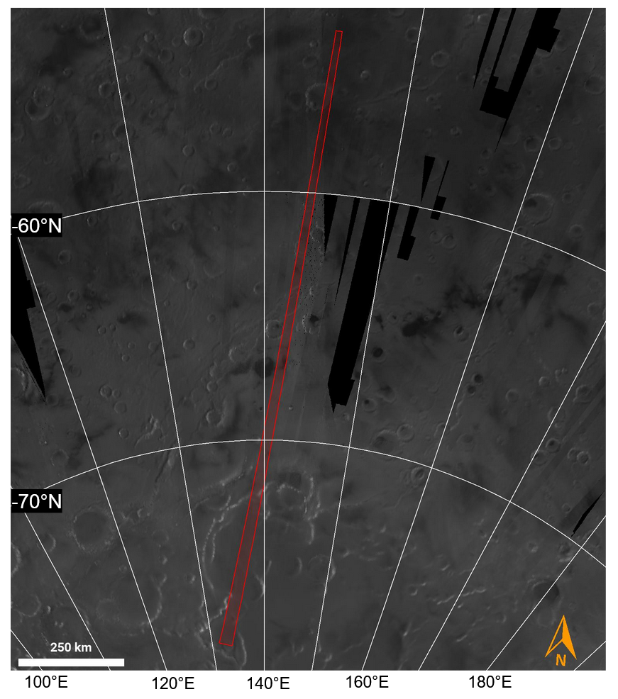
Figure 1: NIR-1 µm Albedo map [9] of the region where the OMEGA cube ORB2209_3 is located (latitude ranges between -53°N to -78°N and longitude between 131°E to 145°E).
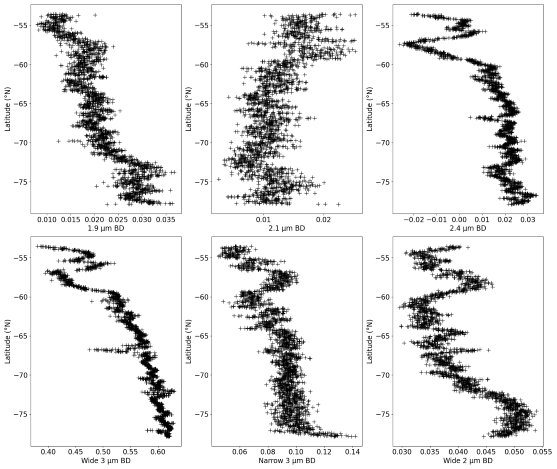
Figure 2: Latitudinal variations of the spectral parameters in the OMEGA cube ORB2209_3 (Figure 1).

Figure 3: Variability of the spectral parameters in the OMEGA cube ORB2209_3 between -53°N to -65°N, from left to right: band depth at 1.9 µm, narrow and wide band depth at 3 µm and 2 µm.
Data availability
The OMEGA/MEx data are freely available on the ESA PSA at https://archives.esac.esa.int/psa/#!Table%20View/OMEGA=instrument. This work uses the OMEGA-Py Python module, freely available on GitHub at https://github.com/AStcherbinine/omegapy.
References
[1] Poulet et al., GRL, 35(20) (2008). [2] Jouglet et al., JGR:Planets 112.E8 (2007). [3] Stcherbinine et al., Icarus, 369, 114627 (2021). [4] Carter et al., Sixth International Conference on Mars Polar Science and Exploration (Vol. 1926, p. 6063) (2016). [5] Langevin et al., Science, 307, 5715 (2005). [6] Viviano-Beck et al., JGR:Planets, 119(6), 1403-1431(2014). [7] Vincendon et al., JGR:Planets 116.E11 (2011). [8] Gendrin et al., Science, 307, 5715, 1587-1591 (2005). [9] Ody et al., JGR:Planets, 117(E11), (2012)
How to cite: Barraud, O., Carter, J., Vincendon, M., and Stcherbinine, A.: Spectral variability of the south polar region of Mars and implications for hydration and sulfate mineralogy, Europlanet Science Congress 2022, Granada, Spain, 18–23 Sep 2022, EPSC2022-847, https://doi.org/10.5194/epsc2022-847, 2022.
1. Introduction
Some terrestrial concretions may be analogs of Martian concretions "blueberries". They were discovered on Mars in the Meridiani Planum area (0°12′N, 357°30′E) by the Opportunity rover. The conditions for the sedimentation of Martian concretions are still unknown. They could have arisen in a similar sedimentation environment as some terrestrial concretions. Therefore, it is important to determine which Earth concretions are analogs of Martian concretions and under what conditions they were formed. This would significantly enrich knowledge about the conditions prevailing on Mars during the formation of Martian concretions, and would be an important evidence for the presence of liquid water in the history of the red planet [1], [2].
2. Concretions from Utah
Near the MDRS (Mars Desert Research Station) base in Utah, USA, sandstone concretions of Cretaceous Dakota Formation were collected. In contrast, the early Jurassic concretions in the Navajo Formation adjacent to Dakota are additionally covered with a thick layer of hematite and other iron compounds. It is known that they crystallized in layers of fine sandstone. As the sandstones were eroded, concretions fell out of them by gravity. Then it can reach to a re-crystallization on the surface of these concretions in a similar way as on the concretions from Jurassic layers of the Navajo Formation from Utah [3], [4].
|
|
|
|
|
Fig.1. A layer of Cretaceous sandstone from the Dakota Formation in Utah with concretions. The size of the visible layer with concretions of about 0.5 m.
|
|
Fig.2. Sandstone concretions of the Cretaceous sandstone of the Dakota Formation in Utah.
|
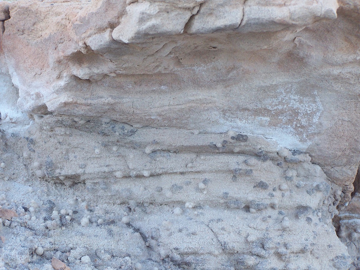
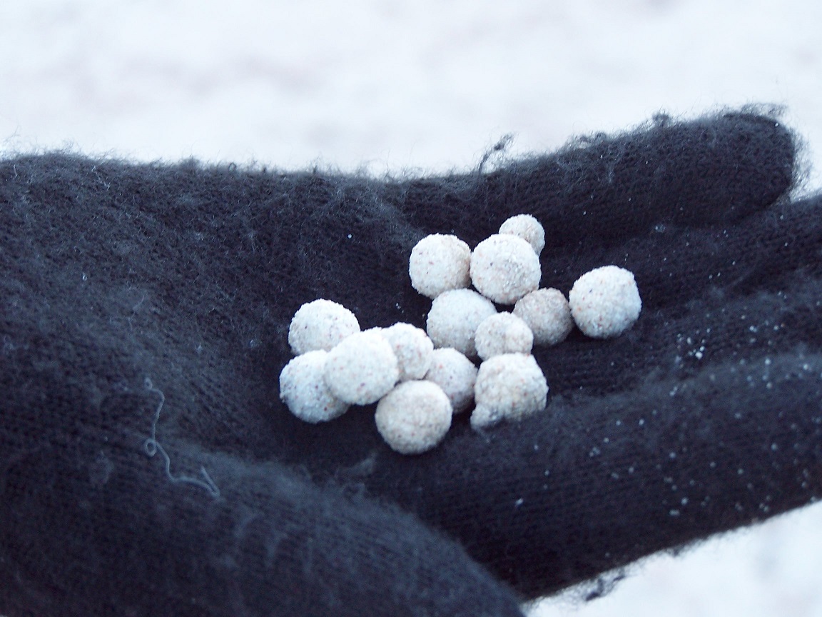
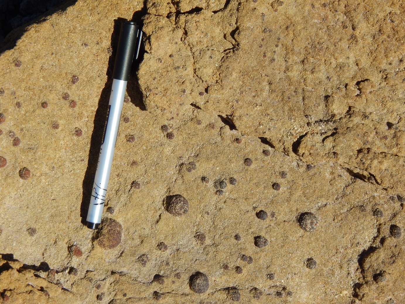
Fig.3. Surface of the Dakota Cretaceous sandstones with distinct mineralization of iron oxides.
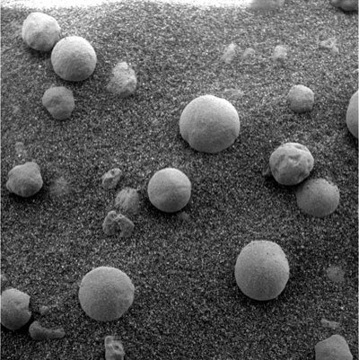
Fig.4. Image from the Microscopic Imager camera showing concretions taken by the Opportunity rover on Meridiani Planum. This image is ~3 cm across and was taken on the 15th day of Opportunity's journey (NASA Feb. 8, 2004).
Figs 1,2 show concretions in the Cretaceous layer, leached by migrating waters and re-mineralized, for which carbonates also contribute [5]. Fig. 3 shows concretions highly mineralized with iron oxides with a large proportion of hematite and goethite. When these concretions fall out by gravity, another mineralization takes place on their surface, in the case of Utah again with iron oxides, which creates a kind of glassy shell on the concretion [6].
In many publications, scientists emphasize that these concretions were formed in presence of water. Their chemical mineralization is quite complex because the water that migrates through the porous sandstones is responsible for the crystallization of these formations thanks to the dissolved chemical compounds. There is a repeated mineralization and demineralization, and therefore the chemical composition of concretions in different regions of the world may differ despite the similar origin of their formation [7], [8], [9].
3. Comparison of spectra
In our research we used the results obtained with the Mossbauer spectrometer for Martian soil with "blueberries", Fig.4, [10]. We identified the minerals likely to be present at the sample. We used appropriate spectra for these minerals from the USGS library and compared them to the infrared spectra of concretions from Utah- Fig.5.
Since the Mossbauer spectrometer does not provide information about all possible minerals because it focuses on minerals containing the Fe element, it is possible that the mineralization of Martian concretions is much richer. Jarosite and hematite discovered by the Mossbauer spectrometer fit well with the bands of the infrared spectra of the Utah concretions. Moreover, the minerals that can be recognized in the spectra of concretions from Utah are also clay minerals and gypsum. The sandstones in which this mineralization took place, of course, contain quartz, but in the short infrared range it has no spectral characteristics, therefore quartz is not visible in the spectrum.
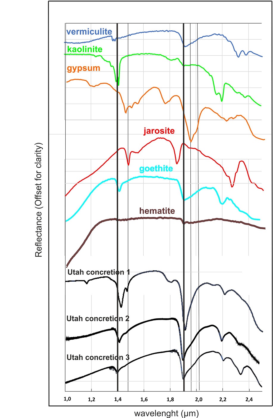
Fig.5. NIR spectra of the Cretaceous Dakota Formation in Utah (spectrometer Nicolet iS50) compared with minerals from the USGS library. The 1.4 and 1.9 µm bands reveal the influence of clay minerals and iron oxides, and additionally sulphates (gypsum and jarosite).
4. Conclusions
We found significant correlation between the Utah concretions of the Dakota Formation and those found by the Opportunity rover. A common feature of these concretions is a similar ferric sulphate mineralization. It follows that Martian and Utah concretions might have formed in an acidic environment and water was important for their formation.
References
[1] Chan, M., et al., (2005) GSA Today, 15, 8, 4-10
[2] Fan, Ch., et al., (2010) Planet. Space Sci., 58, 401–410
[3] Busigny, V., and Dauphas, N., (2007) Earth and Planet. Sci. Let., 254, 272–287
[4] Potter, S., and Chan, M., (2011) Geofluids
[5] Parry, W., (2011) Sediment. Geol., 233, 53-68
[6] Chan, M., et al., (2007) Geofluids, 7, 1–13
[7] Mika, K., et al., (2018) Geofluids of Utah, 47, 197-219
[8] Di Bella, M., et al., (2021) Minerals, 11, 460, 1-18
[9] Ray, D., et al., (2021) Planet. Space Sci., 197, 105163
[10] Klingelhofer, G., et al., (2004) Science, 306, 1740-1745
How to cite: Zalewska, N. and Czechowski, L.: Some remarks about Martian "blueberries" and spherical concretion from Utah, Europlanet Science Congress 2022, Granada, Spain, 18–23 Sep 2022, EPSC2022-737, https://doi.org/10.5194/epsc2022-737, 2022.
1.Introduction
A straight V-shaped channel with two overlapped fan-shaped deposits at the mouth, close to a possible fissure volcano (121.43°N,2.16°E) in Nepenthes Mensae region of Mars (Fig.1) has previously attracted our attention [1]. The MOC-NA and the first HRSC images in the area allowed us to propose a hydrological evolution for the area, including water level variations over time [2]. Now, we revisited the site with higher resolution images and topography to model [3] the mechanisms that created the fan-shaped deposits with a recent methodology [4]. This will expand our understanding of the area's fluvial processes by adding to the debate over variations in water levels at long-standing water bodies. Here we present the preliminary geological observations that will constrain the forward topographic deconstruction and the numerical modeling.
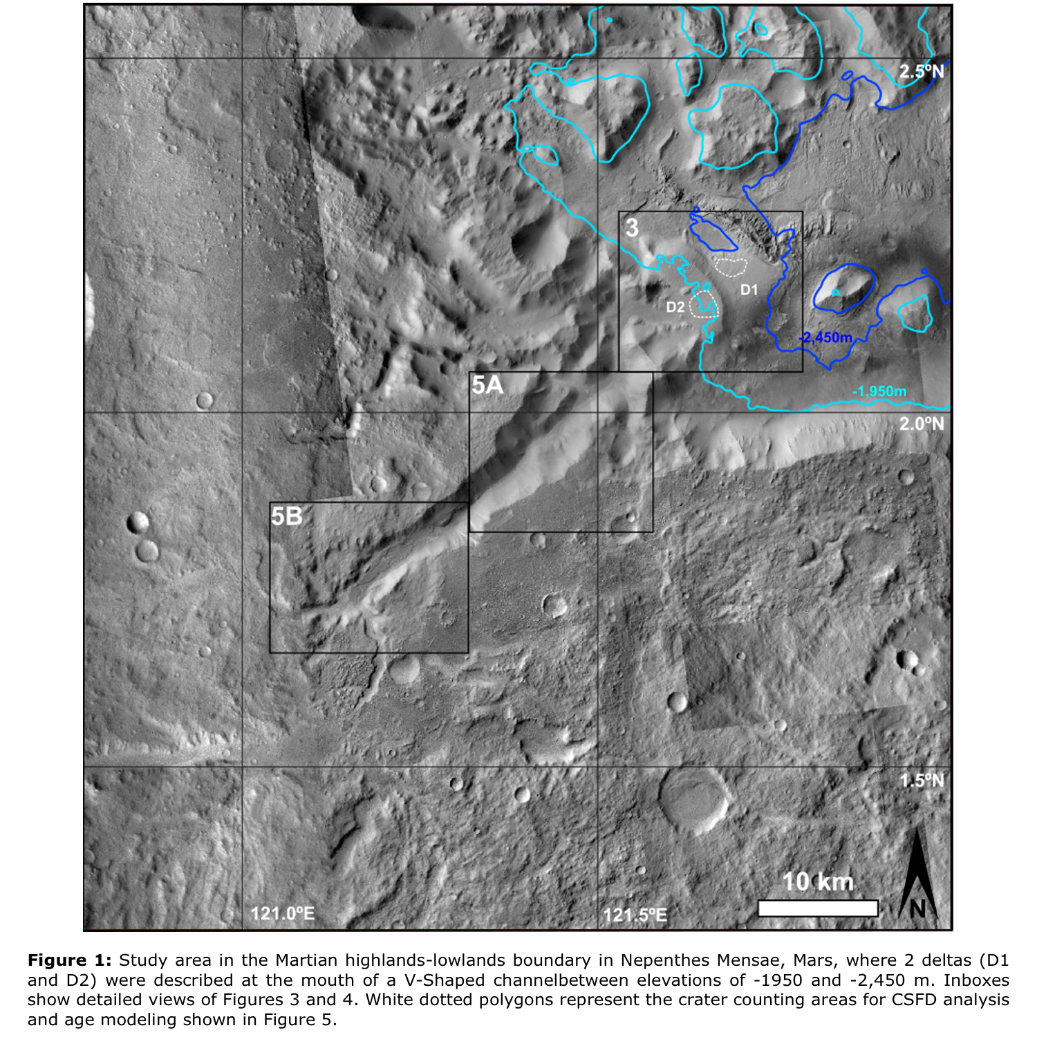
2.Methodology
We plan to reconstruct the hydrogeological evolution of the area using a three-step iterative model (Fig.2,[4]). Starting with the geological study of the area (Fig.2,O1), we used a GIS (QGIS 3.16) with recent imagery (CTX,HiRISE) and topography (HRSC). We refined the previous geomorphological description of the features and dated the two hydrologic events through CSFD analysis using the CraterStats2 software [5]. After identifying topographical constraints for the modeling process [3] we performed a series of topographic deconstructions (Fig.2,O2) that would be the input for the numerical modeling (Fig.2,O3).
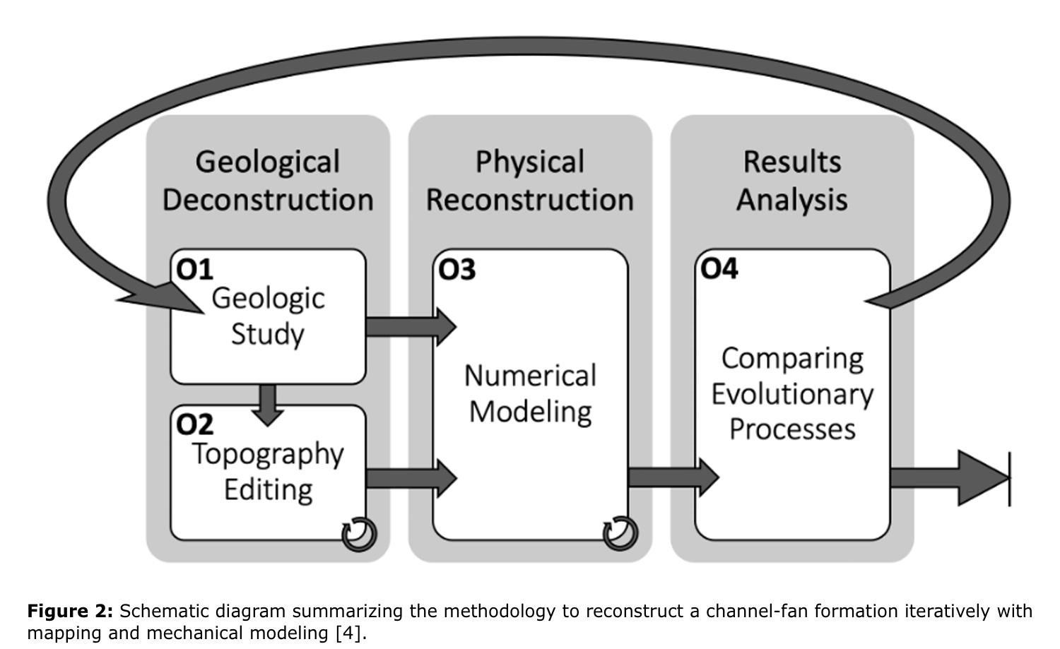
2.1.Geological Deconstruction
2.1.1.Geologic study
Two major fluvial phases were proposed at first based on the appearance of two overlapped deltas [2]. The first, resulting in the formation of an alluvial fan at the bottom (D1), could have formed in the absence of a standing water table; the second, a pristine Gilbert-type delta (D2), could have formed at roughly -1,990 to -1,950m elevation water table [2,6]. According to HRSC-derived topography, the base of D1 is at around -2,540m elevation (Fig.1), and Contact 1 of Oceanus Borealis is at about -2,499m elevation [7,8]. This could support the hypothesis that D1 originated as an alluvial fan near the water's edge.
Other deposits at the base of both deltas are visible on high-resolution images, which could result from prior fluvial processes (Fig.3). The images demonstrate the presence of other distal deposits between the two deltas (Fig.3), most likely due to the gradual rise of the water table, resulting in a reduction in the areal extension of the deposits while they increase in thickness. The presence of benches at elevations ranging from -1,400 to -2,400m [2,6] may indicate a progressive change in the water table level.
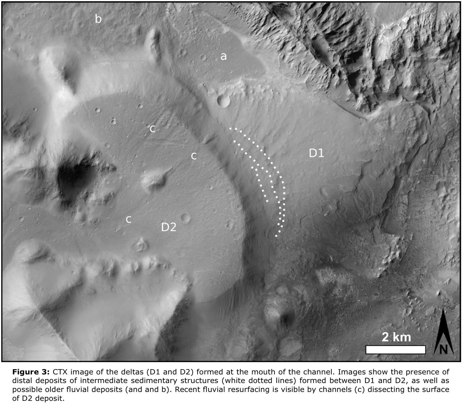
The CSFD analysis allowed both deltas to be dated (Fig.4). Due to resurfacing events, D1 does not reveal ages older than 400Ma (400 and 84Ma). Since ages of 3.5 and 3Ga have been fitted, D2 was produced in Hesperian. Other ages of 820 and 63Ma are produced by resurfacing processes. Although we found younger resurfacing ages, the age of creation of D2 fits with the age of other deltas in the vicinity [6]. Resurfacing activities and aeolian events are aided by channels slicing the top surface of D2 (Fig.3).
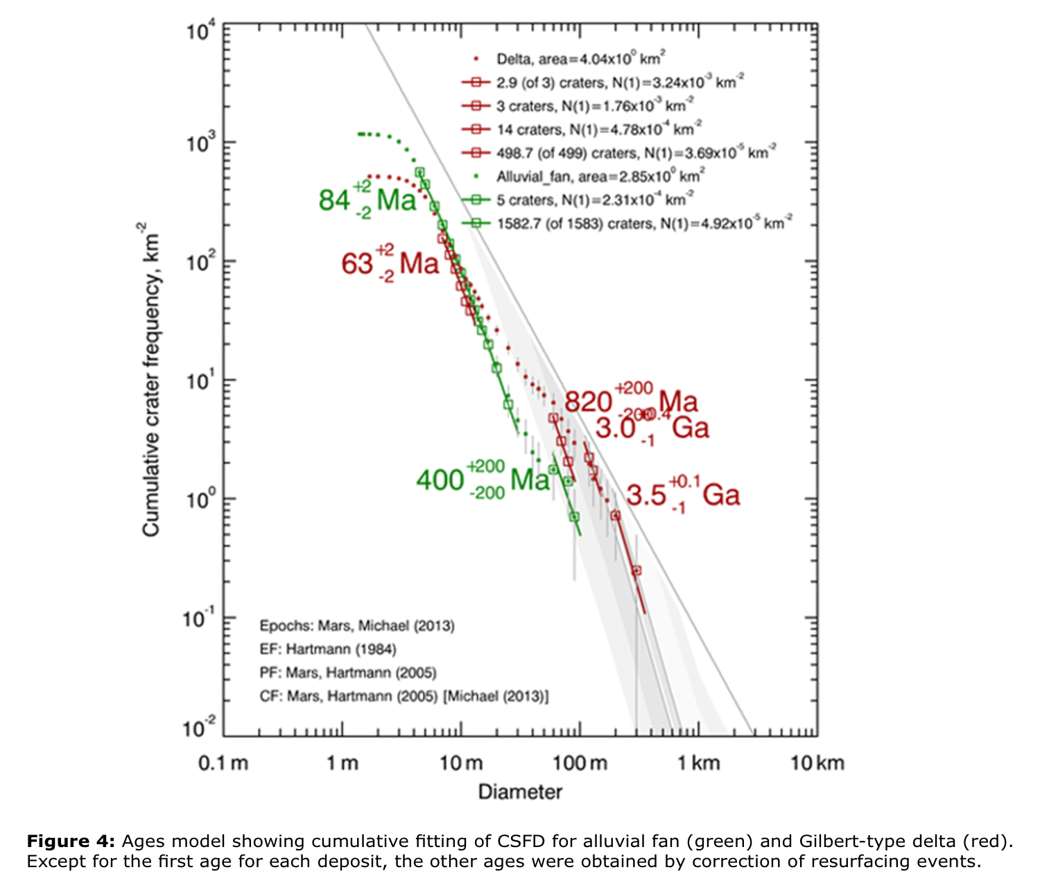
These sedimentary deposits were made possible by materials carried by a river flow after excavating a V-shaped valley, which is now filled with fluvial, aeolian, and sediments from mass-wasting processes, such as a rotational landslide (Fig.5A). A probable fluvial terrace was presented [2]; however, it could not be now validated using high-resolution images. Other features, such as two knickpoints, are now visible (Fig.5B), indicating (1) the presence of resistant material acting as local base levels or (2) the decline of water table levels at the channel mouth [9]. Also evident are sedimentary deposits at the top section of the channel, as well as along the degraded channels, such as those coming from the tributary, which gives a key to reconstructing the sequence of fluvial events in this system.
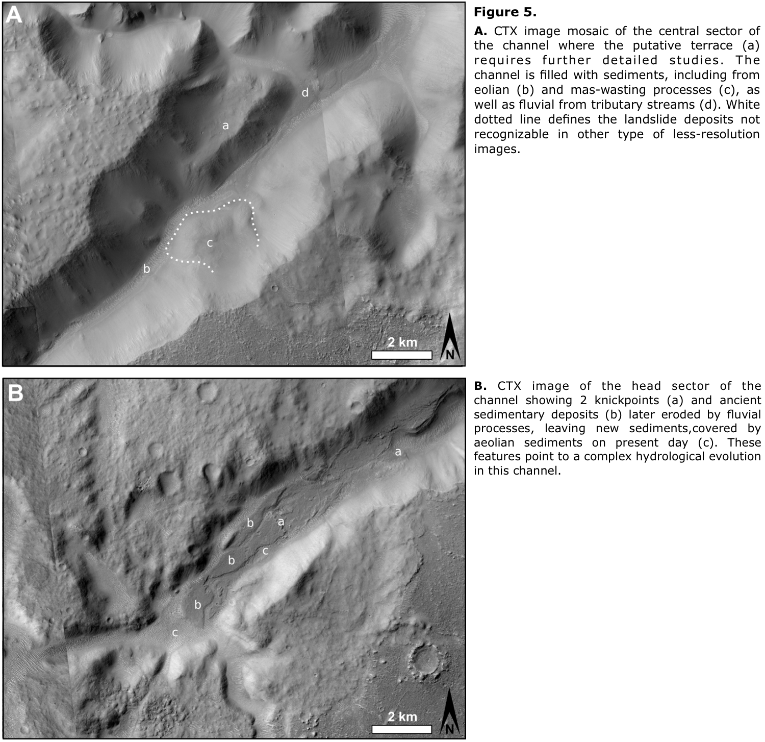
2.1.2.Topography editing
Having differentiated the phases for the formation of hydric geomorphologies, their characteristics, and the extent of other subsequent processes altering the relief, we modified the topography to emulate the one prior to the hydrological process, also determining the position and volume of the mobilized material. We tested the different working hypotheses with different deconstructions that will be iteratively refined.
2.2.Physical reconstruction: Numerical Modeling
The initial conditions and topographies are extracted from the geological deconstruction, which must be interpolated in a computational mesh (Fig.6). Subsequently, a two-phase (i.e., soil and water) model based on the depth-integrated Navier-Stokes equations will be applied [10].
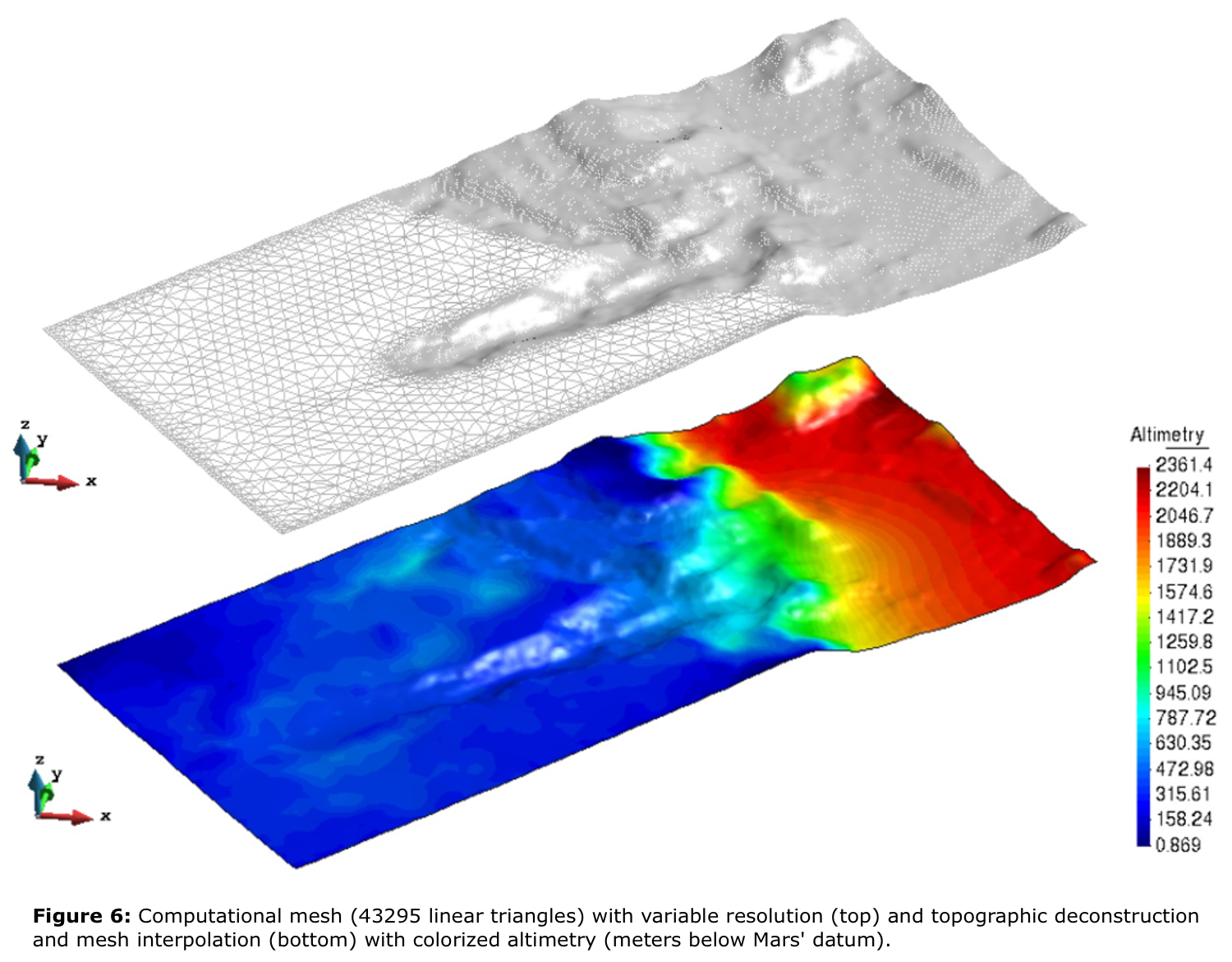
The simulations will provide the volume of mobilized material, type of material (including its water content), a final topography, and the duration time of the event to be studied [3].
2.3.Results Analysis
A comparison of the evolutionary processes by evaluating the differences found between the simulation results and the studied morphologies in terms of volumes of mobilized material, flow directions, final slopes, and shape will be accomplished. Based on the discrepancies obtained, it will be decided whether the iterative process must be finalized or a new deconstruction/reconstruction process must be started.
3.Expected results
This methodology will provide a better understanding of the hydrogeological processes that lead to the formation of the deltas in Nepenthes. Information about the water content, duration of the processes, and the existence (or not) of a layer of water in the lowlands will be obtained.
Besides, the proposed technique can be applied elsewhere on the surface of Mars, being possible to extend it to the study of other geological processes and even other planetary bodies. In this way, this study will help shed light on how and when the geological and environmental evolution of Mars has taken place.
Acknowledgements
The authors thank the AEI projects PID2019-107442RB-C32 and MDM-2017-0737.
References
[1]de Pablo and Pacifici, 2006. EPSC2006-A-00447. https://adsabs.harvard.edu/pdf/2006epsc.conf..447D
[2]de Pablo and Pacifici, 2008. Icarus, 196(2):667-671.https://10.1016/j.icarus.2008.04.005
[3]Herreros et al., 2021. EPSC2021-116.https://doi.org/10.5194/epsc2021-116.
[4]Molina et al., 2021. EPSC2021-129.https://doi.org/10.5194/epsc2021-129.
[5]Michael and Neukum, 2010.https://10.1016/j.epsl.2009.12.041.
[6]Arnay and Gutiérrez, 2020. Geomorphology, 359. 10719.https://doi.org/10.1016/j.geomorph.2020.107129.
[7]Clifford and Parker, 2001. Icarus 154, 40-79.https://doi:10.1006/icar.2001.6671.
[8]Di Achille and Hynek, 2010. Nature Geoscience 3, 459-463.https://doi.org/10.1038/ngeo891.
[9]Durán et al., 2019. Sci Rep 9, 15153.https://doi.org/10.1038/s41598-019-51574-2.
[10]Pastor et al., 2009. Engineering Geology, 109(1–2): 124-134. https://10.1144/1470-9236/04-038.
How to cite: Molina, A., de Pablo, M. Á., Herreros, I., Pertuz Domínguez, A., Roldán Caselles, G., and Martínez, A.: Modeling of fluvial episodic events at a channel in Nepenthes Mensae region of Mars, Europlanet Science Congress 2022, Granada, Spain, 18–23 Sep 2022, EPSC2022-413, https://doi.org/10.5194/epsc2022-413, 2022.
Introduction: Inverted channels are sinuous ridges comprising fluvial facies, which have gained a positive relief due to differential erosion [e.g., 1, 2]. Many have been found preserved on Mars in terrains dated between the Mid-Noachian to Early Hesperian in the region of Arabia Terra [1, 3, 4]. The distribution of these features is well known [e.g., 2, 3] but timing, geological settings, their relative timescales of liquid water stability and the nature of the early climate under which fluvial deposition was possible are still under debate. We present results from studies conducted on three morphologically different inverted channel systems in the region of Arabia Terra: Arago Dorsa (within the Arago crater), Cantabras Dorsum and Piscinas Serpentes (in Meridiani Planum). The analysis includes interpretations of the formation settings of the three systems and estimation of the volume of preserved alluvial materials and the consequent required period of fluvial activity for such deposition.
Methodology: Digital morphostratigraphic maps (scale 1:10,000) were constructed using ArcGIS software using 25 cm/pixel HiRISE images [5]. A CTX mosaic [6] was used to study the general context of the study area, and to assist the analysis of stratigraphy. HiRISE DEMs [7] were used to calculate thicknesses of units interpreted as fluvial facies and to characterise and interpret the stratigraphic relationships of the different geological units. When HiRISE DEMS were not available, the HRSC-MOLA DEM [8] was used. The ridges’ morphometric parameters (length, thickness, width) were used to estimate both the preserved volume of alluvial material and the duration of fluvial activity of the systems, assuming sedimentation rates of 0.01-0.7 m/Kyr from terrestrial comparisons [4, 9].
Inverted channel types and settings: The Arago Dorsa ridges are the result of channel belt aggradation [10], as shown by the presence of a well-organized multi-level structure made of candidate channel fills and overbank deposits. We interpret the overall structure as a candidate relict aggrading fluvial fan preserved within a continental highland basin in a distal portion from the source where inverted channel belts are usually formed [11]. Cantabras Dorsum represents a complex package of fluvial sediments, and presents two distinct ridges. The smaller, a sinuous flat-topped ridge with a rectangular cross-section [following 2], is developed on top of a wider one (Fig. 1). We interpret the structure as alluvial deposits deposited by an avulsed channel on the floor of a wider valley which progressively reduced the cross-sectional area, terminating in a smaller channel now expressed by the upper inverted ridge. Piscinas Serpentes presents a network of fine-scale valleys that transition downstream (north of the studied site) into pitted channels and finally ridges (Fig. 2). The ridges of Piscinas Serpentes, are more likely the result of channel fill in a ribbon-like channel.
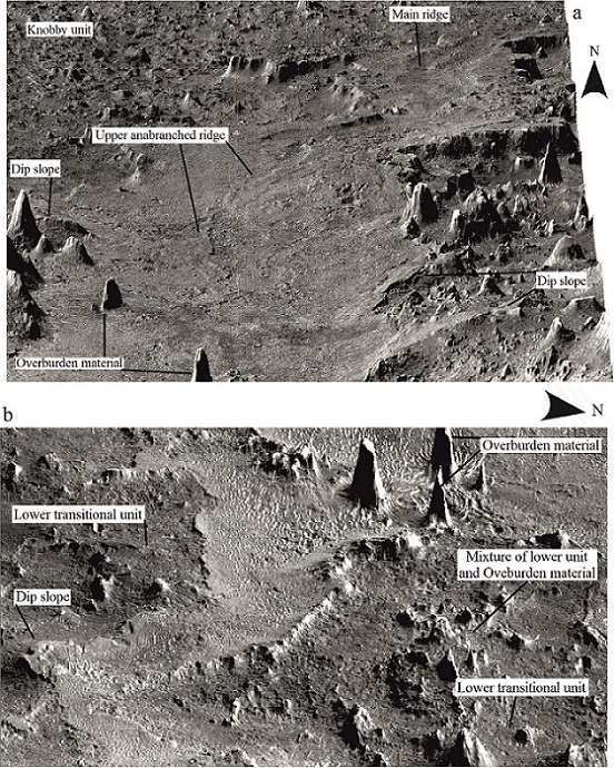
Figure 1: HiRISE-DEM oblique view of Cantabras Dorsum. Vertical exaggeration = 5 times. a- Main ridge (9.13°N, -5.47°E). b- Lateral oblique view of the upper ridge (9.13°N, -5.48°E).
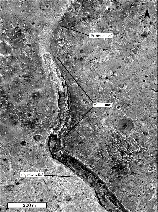
Figure 2: Detail of Piscinas Serpentes system (ESP_048489_1845; 4.51°N, -1.17°E), where the passage from positive inverted relief in the northern part of the image to negative relief in the south is visible.
Estimation of volume and timing for fluvial deposition: The estimated vertical thickness of the ridges and the estimated duration of fluvial activity (Table 1) are in line with those measured for terrestrial analogues [12]. Aggrading systems like Arago Dorsa and Cantabras Dorsum should have been stable for between 104-106 years.
Table 1: Morphometric data of the studied systems and estimation of volume and formation timescale of fluvial activity.
|
System |
Vertical Thickness (m) |
Exposed Length (m) |
Width (m) |
Volume of alluvial material preserved (km3) |
Terrestrial analogues sedimentation rates (m/kyr) |
Formation time scale (Myr) |
Approximate fluvial activity (Yr) |
|
Arago Dorsa |
50 |
25,000 |
18,000 |
22.5 |
0.01–0.7 |
0.07-5 |
105-106 |
|
Cantabras Dorsum |
35 |
100,000 |
2000 |
7 |
0.01–0.7 |
0.05-3.5 |
104-106 |
|
Piscinas Serpentes |
10 |
10,000 |
90 |
0.009 |
0.01–0.7 |
0.01-1 |
104-106 |
Conclusions and implications for martian climate: Our study supports long-duration fluvial and aqueous inputs to allow significant thicknesses of fluvial aggradations and/or avulsions to occur in a variety of settings across Arabia Terra (a crater/basin and valleys). It also shows a distributed source of water in Arabia Terra. Geological settings where inverted relief developed, their morphometry and the estimated formation time are similar to terrestrial analogues [12], suggesting that similar environmental conditions are likely to have characterised the two planets at the time of fluvial activity. The obtained results are better explained with a stable hydrological cycle which would have been required to allow migration and aggradation in such a large region, probably sourced from precipitation both in the area and upstream.
References: [1] Davis et al., (2019), JGR Planets, 10.1029/2019JE005976. [2] Mirino et al.,(2020), LPSC 2020, LPI Contribution No. 2326, 2020, id.1492. [3] Davis et al., (2016), Geology, G38247.1. [4] Balme et al.,(2020), JGR Planets, https://doi.org/10.1029/2019JE006244. [5] McEwen et al., (2007), JGR, 112:E05S02. [6] Dickson et al., (2018), LPSC 2018, LPI Contrib. No. 2083. [7] Davis (2019), https://doi.org/10.6084/m9.figshare.c.4330838.v1. [8] Fergason et al., (2018). U.S. Geological Survey, http://bit.ly/HRSC_MOLA_Blend_v0. [9] Colombera et al., (2015), Geology, 10.1130/G36385.1. [10] Mirino et al., (2021), EPSC 2021, https://doi.org/10.5194/epsc2021-311, 2021. [11] Ventra & Clarke (2018), Geological Society of London, 10.1144/SP440.16. [12] Zaki et al., (2021), Earth-Science Reviews, https://doi.org/10.1016/j.earscirev.2021.103561.
How to cite: Mirino, M., Balme, M., Fawdon, P., and Grindrod, P.: Evaluation of style, settings and timing of martian fluvial deposition troughs inverted channel studies., Europlanet Science Congress 2022, Granada, Spain, 18–23 Sep 2022, EPSC2022-559, https://doi.org/10.5194/epsc2022-559, 2022.
Introduction: Inverted landforms are positive relief and well-preserved features; typically, their formation instigated by deposition of sediments by fluvial activity and later exhumed by aeolian activity [1-3]. Their forming material offers greater resistance to erosion than the surrounding, thus produces the inverted relief [3]. On Mars, inverted landforms retained the records of paleo-environment in the form of inverted channels [1,2] and potential inverted fans, though the latter is still to confirm.
Fluvial activity is widely reported on Mars and possesses a long-time span from Noachian to Hesperian period [4]; a few reports [5,6] suggest continuation to early Amazonian epoch. However, episodes of fluvial activities during the younger epochs and effects of local environment are still uncertain. A better understanding of formation conditions and epochs of inverted landforms can yield insights into their development and paleo-climatic conditions prevailed on Mars. This study focused on inverted landforms present within an unnamed crater (centered at 22.8°N, 175.9°E), located in the north-west of Orcus Patera on Mars [Fig 1].
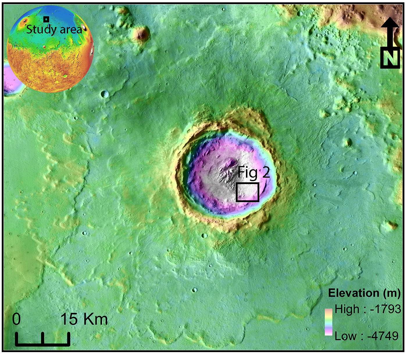
Fig 1: Unnamed crater with visible ejecta boundary. MOLA-HRSC DEM overliad CTX-mosaic.
Data and Methods: HRSC-MOLA blended DEM [7] and MRO-CTX mosaic [8] data were used for the preliminarily topographical and, morphological and chronological analysis respectively. For the detailed analysis of the stratigraphy and morphology, high-resolution HiRISE DEM generated using MarsSI [9] with HiRISE [10] and CaSSIS color [11] images were used respectively.
Results and Discussion: Within this unnamed crater the inverted landforms are located in the south-west region [Fig 1]. We observed that the southern wall is carved by fluvial channels associated with inverted channels towards the floor [Fig 2]. This clearly shows transition from negative-relief fluvial channels to positive-relief inverted channels. The thickness of the inverted channels is observed to vary from ~5 m to ~12 m. We also observed the association of inverted channels with triangular-shaped deposits on the crater floor [Fig 2]. These deposits typically appear like fan shape and herein interpreted as potential inverted fans [Fig 2]. The formation of these fans may have initiated by the deposition of sediments carried by flowing water and later erosion of the surrounding terrain by wind. Interestingly, these fans show superposition relationship from right to left (younger to older) in Fig 2. We identified at least three clear superposition relationships [Fig 2], thus likely suggest three or more episodes of water-flowing activity in this crater on Mars or multiple deposits occurred at the same time.
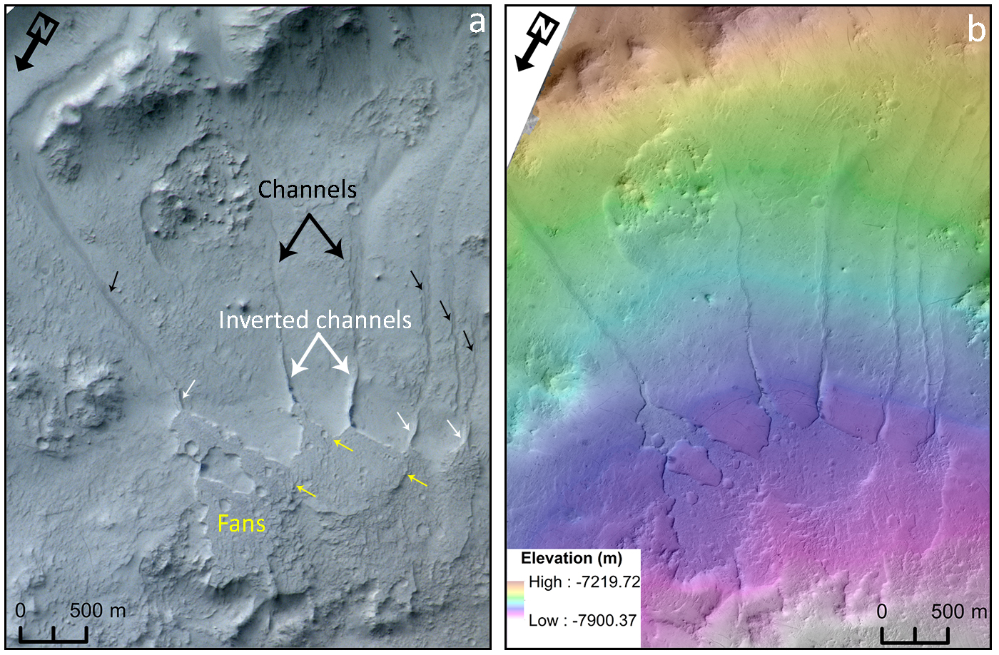
Fig 2: a) CaSSIS color image showing transition from negative-relief channels (black arrow) to positive-relief inverted channels (white arrow) with associated fans showing superposed relationship (yellow arrow). b) HiRISE DEM overlayed on HiRISE image to show topography.
Further, to determine the period of fluvial activity within this crater, we determined the modelled absolute age of the crater by computing the crater-size frequency distribution of the primary craters on the ejecta of studied crater [Fig 3]. The crater-size frequency distribution for the unnamed crater [Fig 3b] suggests an age of ~1.9 Ga (mid to late Amazonian epoch) using the CF and PF from Hartmann and Neukum (2001) and Ivanov (2001) respectively. Thus, we interpret that the inverted channels and potential inverted fans formed post to ~1.9 Ga on Mars.
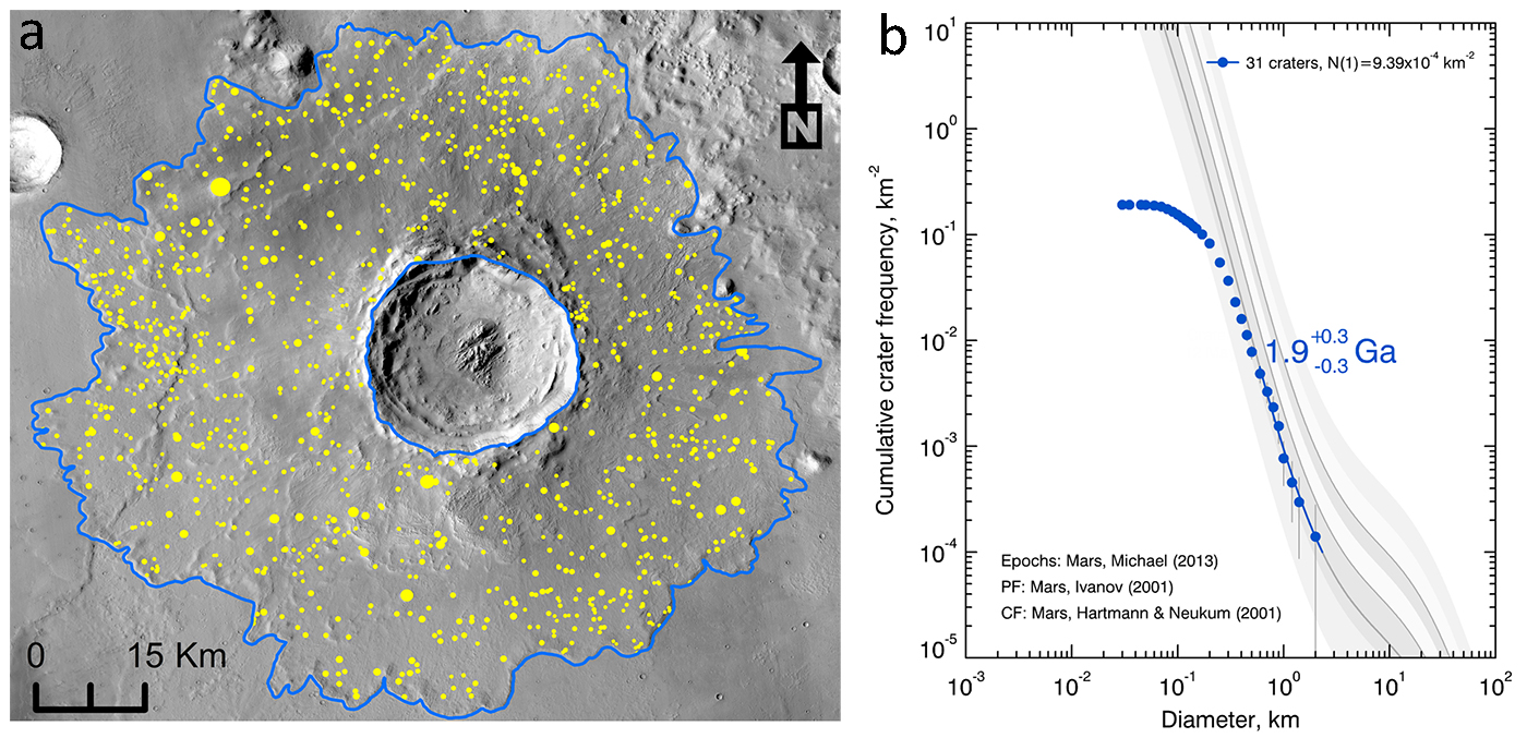
Fig 3: a) Counted superposed craters (yellow) over the ejecta (blue) of studied crater for age determination. b) CSFD plot showing the best fir age of the unnamed crater.
Summary: This study demonstrates that the inverted landforms in the unnamed crater formed post to 1.9 Ga and thus recommends recent fluvial activity on Mars within the last 2 billion years. In addition, multiple superposition relationship of fans on one-another suggests that the fluvial activity was periodic in nature and at least three episodes of water flowing activity occurred in this crater. Thus, this location on Mars hosts evidence for recent and possibly recurring fluvial activity and likely have astrobiological importance. Analysis for the origin and source of water is ongoing and this may hint for the local paleo-environmental conditions prevailed on Mars.
Acknowledgments: The authors wish to acknowledge the teams of CaSSIS, HiRISE, CTX, MOLA and HRSC. Harish and MRELM acknowledge support for this work through an internal grant (8474000336-KU-SPSC).
References: [1] Jacobsen and Burr (2017), Geosphere, 13, 2154–2168. [2] Davis et al., (2016), Geology, G38247.1. [3] Zaki et al., (2018), Icarus, 309, 105-124. [4] Carr and Head (2012), EPSL, 294, 185-203. [5] Vijayan and Sinha (2017), JGR Planets, 122, 917-949. [6] Harish et al., (2021), 361, 114397. [7] Fergason et al., (2018), USGS. [8] Dickson et al., (2018), 49th LPSC, 2480. [9] McEwen et al., (2007), JGR Planets, 112, E05S02. [10] Malin et al., (2007), JGR Planets, 112, E05S04. [11] Thomas et al., (2017), SSR, 212, 1897-1944.
How to cite: Harish, , Sivaprahasam, V., and El-Maarry, M. R.: Multiple superposed inverted landforms on Mars, Europlanet Science Congress 2022, Granada, Spain, 18–23 Sep 2022, EPSC2022-772, https://doi.org/10.5194/epsc2022-772, 2022.
Introduction
Inverted channel deposits or sinuous ridges are common on the Late-Noachian Early-Hesperian terrains on Mars[1,2]. These exhumed ribbon-like, sinuous sedimentary ridges have been interpreted to be evidence of existence of liquid water on early warm and wet Mars. In addition, these ridges have been interpreted to form as either: 1) short duration single-thread fluvial systems, likely from a single flow event[3] or 2) longer duration multi-thread systems which form channel-belt structure[4]. While single-thread systems more closely preserve the actual geomorphology of the fluvial system, the longer period of duration for the channel-belt systems makes it more conducive for ancient habitability. However, the channel-belt structure is inherently complex, preserving an interplay of contrasting lithologies and flow conditions over relatively longer periods of time. Considering these sinuous ridges are also sampling targets for rovers such as NASA’s Perseverance mission[5], a detailed sedimentary analysis of preserved stratigraphy is important to understand the spatio-temporal distribution of architectural elements. Since in-situ observations of these ridges from Mars is still limited, sedimentology of Earth-based exhumed channel-belt deposits can be an important tool for reconstruction of long-lived fluvial processes on Martian surface.
Data and Methods
For this study, we rely on a combination of field-based observations from Earth and satellite image and topographic datasets from Mars. One of the best preserved sinuous ridge structures on Earth in the Oligo-Miocene Caspe Formation, Spain was utilized as a Terrestrial analogue. The sinuous ridges here formed a part of Guadalope-Matarranya fan that developed in an endorheic Ebro basin[6]. For the purpose of sedimentological analysis, detailed photopanel interpretation (recording detailed facies and architectural observations) was carried out at different roadcut outcrops, which provided a view nearly orthogonal to the axes of the ridges. This was supplemented with secondary observations in longitudinal view, parallel to the axes of the ridge. To compare this with Martian examples, 25–50 cm/pixel HiRISE[7] orthomosaics and derived DEMs were utilized to construct 3D models and conceptual architectural models were prepared for similar sinuous ridges on Mars at Hypanis fan, Eberswalde fan and Aram Dorsum.
Results and Discussions
In our example from Spain, we record that the extensive three-dimensional exposures exhibit facies relationships and sedimentary structures indicative of an amalgamated multistory sand bodies formed due to stacked sandstone bodies separated by erosional surfaces. Each individual story was interpreted to represent singular channel unit. These could be divided into thicker sandstone comprised channel-axis complexes and either associated or truncated thinner channel-wing complexes which extend into the floodplain horizon and preserve abundant floodplain mudstone between two such channel-wings. In addition, on each ridge face, three hierarchal surfaces were identified - Channel-bounding Surfaces, Bar-bounding Surfaces and Accretion surfaces. The nearly orthogonal ridge view also preserved the saw-tooth edges, which are commonly associated with reoccupational stacking where channels avulse and occupy previous channel locations[8].
Individual elements of this observed stratigraphy in the field are similar to those reported on Mars [e.g. 9]. These field based observations were used to prepare the conceptual models in form of synthetic cross-sections for Martian sinuous ridges and fluvial channel systems. With HiRISE mosaics, we identified key sedimentary features, such as point bars, recessive and protruding layering on the side of the ridges, etc and associated them with elevation data to identify possible distribution of architectural elements within the Martian sinuous ridges. This is helpful in understanding and predicting the distribution structures and lithologies, especially the finer-grained floodplain lithologies, which are important astrobiological targets. The structure of stacking within the Martian ridges also has important implications for usage of ridge elements in paleohydraulic reconstructions.
References
[1] Tanaka et al.,(2014), Geologic Map of Mars: USGS Scientific Investigations Series Map 3292, scale 1:20,000,000, pamphlet 43 p. [2] Carr et al., (2010), Earth and Planetary Science Letters 294(3-4), pp.185-203. [3] Zaki et al., (2022), Journal of Geophysical Research: Planets, 127, e2021JE007087. [3] Hayden et al., (2019), Icarus, 332, pp.92-110. [5] Farley et al., (2020) Space Science Reviews, 216(8), pp.1-41. [6] Cuevas Martinez et al., (2010), Sedimentology, 57(1), pp.162-189. [7] McEwen et al., (2007) Journal of Geophysical Research: Planets, 112(E5). [8] Chamberlin and Hajek, (2015) Journal of Sedimentary Research, 85(2), pp.82-94. [9] Skinner Jr et al., (2021), Icarus, 354, p.114071.
How to cite: Sangwan, K. S., Barnes, R., Davis, J. M., Gupta, S., and Zaki, A. S.: Structure of channel-belt deposits within sinuous ridges on Earth and Mars, Europlanet Science Congress 2022, Granada, Spain, 18–23 Sep 2022, EPSC2022-1123, https://doi.org/10.5194/epsc2022-1123, 2022.
Introduction: Fresh Shallow Valleys (FSVs) are relatively undegraded dominantly mid-latitude valleys and valley networks that are generally shallowly incised (<20 m). into mantle substrate [1]. They are primarily of Hesperian to Amazonian age and are found in the mid-latitudes (30-50° N/S). The primary interpretation is formation through surface runoff of snowmelt, although a sub-ice hypothesis has been suggested for some crater-interior FSVs [2]. Exit-breach craters (EBCs), or pollywog craters, are relatively fresh craters primarily in the 1-7 km diameter range with no contributing drainage beyond the rim, and one or more exit valleys [1, 3].
Observations: Systematic ArcGIS mapping of FSVs and EBCs was conducted in the southern mid-latitudes using the Murray Lab CTX mosaic at a 1:100,000 scale. Of 1668 craters mapped as possible EBCs, 435 of these were designated as firm detections by having evident rim incision, visibly incised valleys, and no exterior contributing drainage. FSVs were mapped only exterior to craters, although many interior crater rims are dissected by FSV-like valleys. A total of 7276 FSVs were mapped averaging 7.2 km in length. Fig. 1a shows the latitudinal distribution of FSVs and EBCs and Fig. 1b the size distribution of EBCs. FSVs and EBCs have similar latitudinal distribution. To assess the possible hydrology of FSVs and EBCs, topographic relationships were analyzed using CTX and HRSC DTMs.
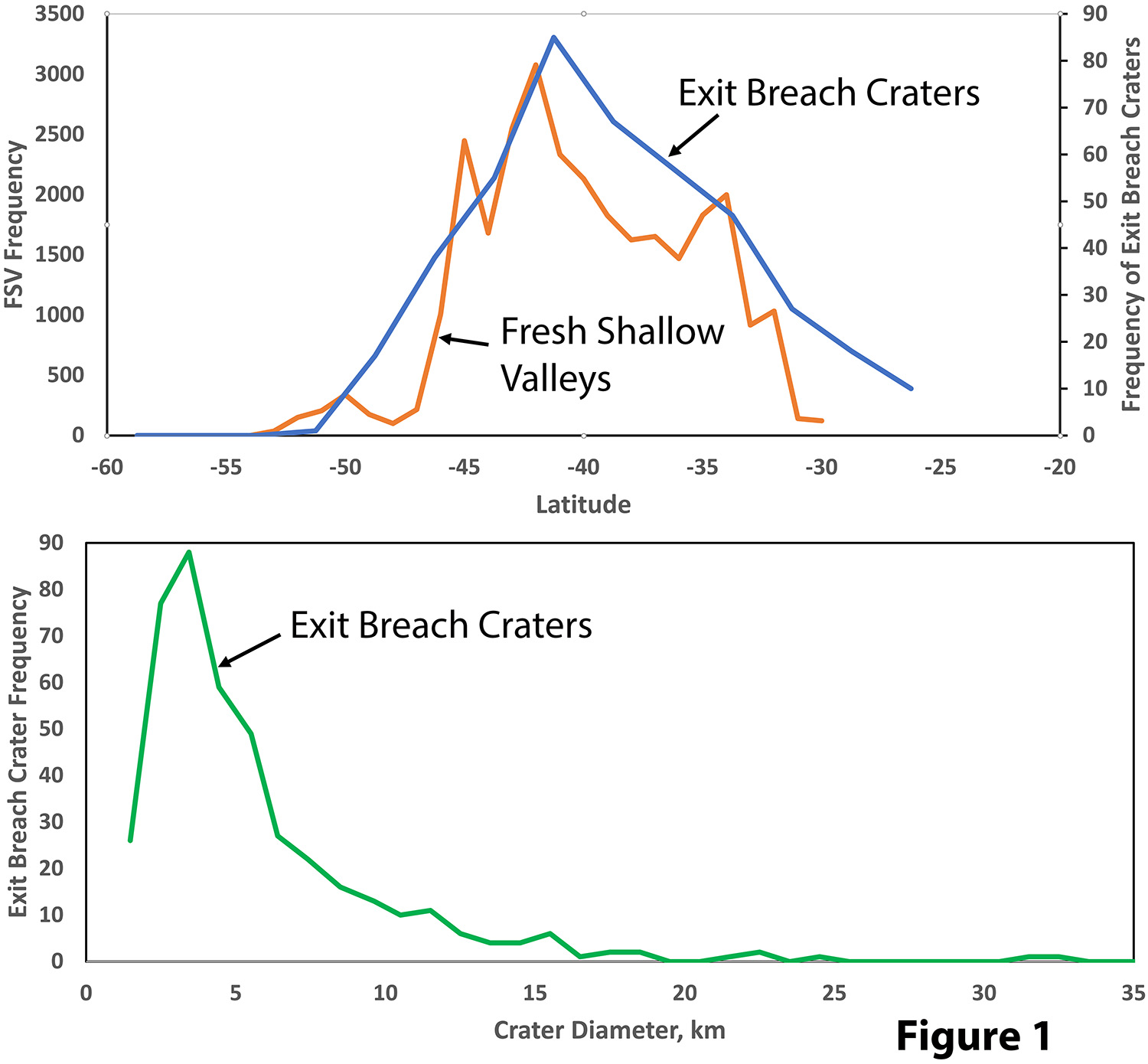
The most deeply incised FSVs occur across divides in settings connecting intercrater basins or connecting intercrater basins to crater interiors (Figs. 2 and 3). Fig. 2 shows FSVs on the northeast exterior rim of a 46 km diameter crater at 44.3°S, 165.2°W. The interior of the crater is indicated by “#”. A ~1 km wide valley leads from the exterior crater rim northward (white arrow). Three ~150m wide FSVs (“a”, “b” & “c”) extend from the valley axis east and northeast with gradients of about 0.04. Each of these FSVs breach the eastern rim of the north-trending valley. The depression on the exterior crater rim at “x” is drained by at least five east-trending FSVs that incise a low ejecta ridge.
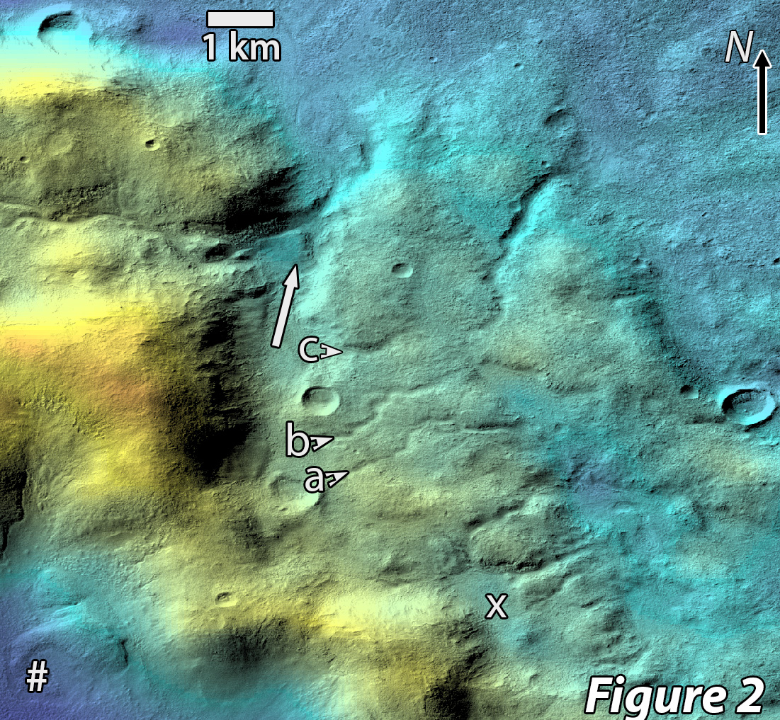
Fig. 3 is centered on the southeastern exterior rim of the same crater. Part of the crater rim is at “#”. The exterior rim depression “d” was drained by two FSVs, one of which extends to the rim depression at “a”. This basin in turn was drained by the FSV shown at the arrow, which incises through an exterior rim ridge at “b”. The lowpoint of the southern rim of basin “a” is at “c”, which is about 30 m lower that the elevation of the FSV rim breach at “b”.
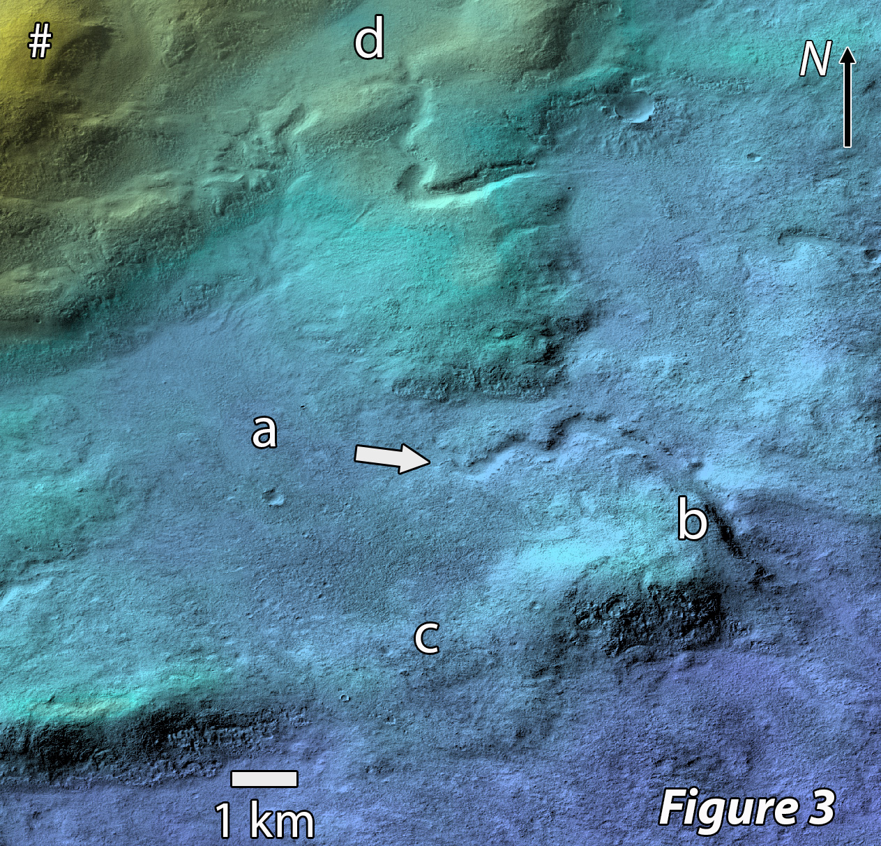
Most EBCs have a single exit breach, but some have multiple breaches. Fig. 4 shows an exit breach crater at 120.56°W, 43.88°S with a minimum of three exit breaches and possibly as many as seven.
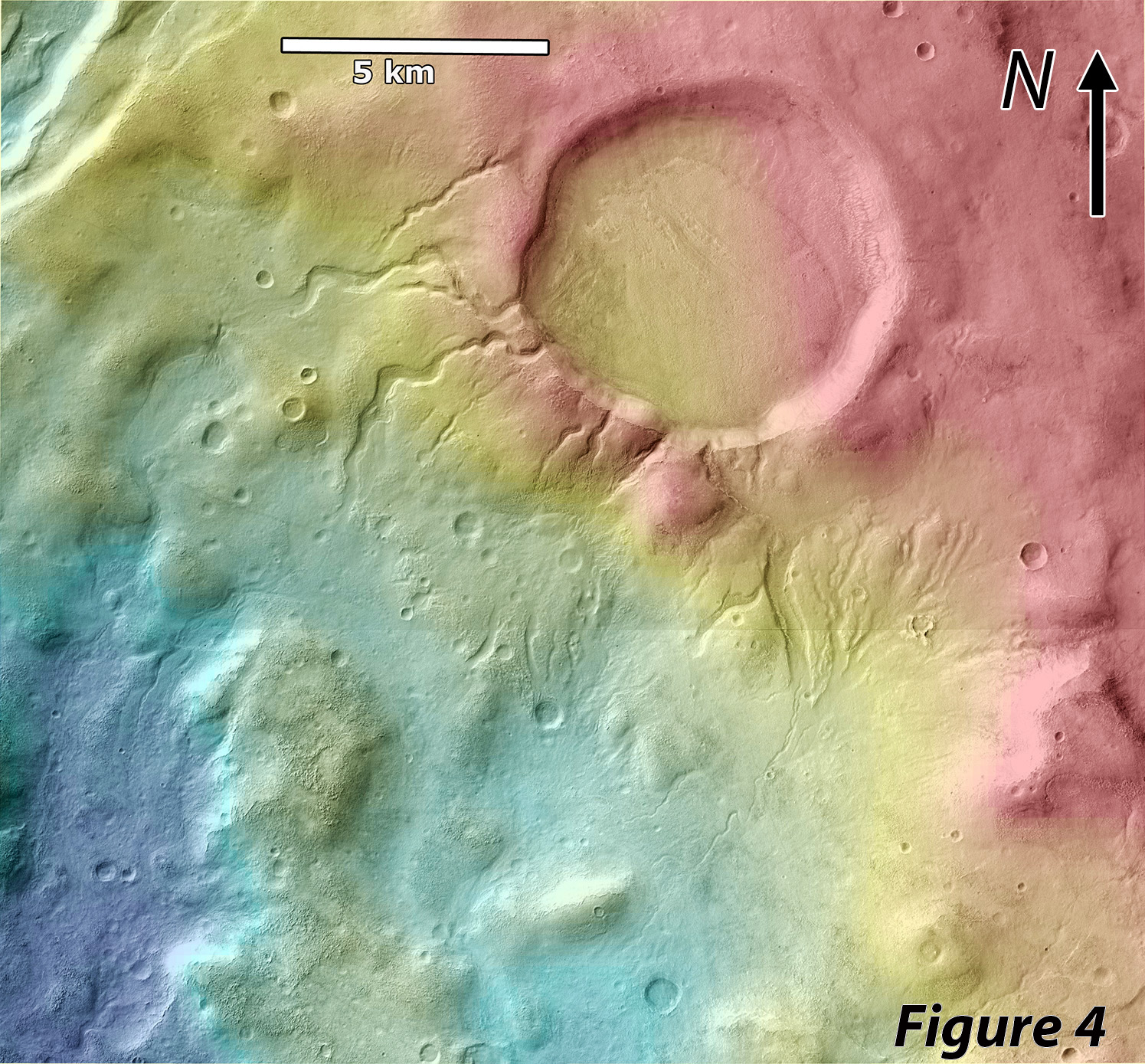
Analysis and Conclusions:
FSV morphology is distinct from typical terrestrial and the older martian valley networks: 1) they are mostly shallowly incised; 2) they are often isolated features; 3) depth of dissection is <20 m unless they cross divides; 4) many display sinuous planforms; 5) FSVs commonly connect basins across topographic divides, often through multiple breaches and extending to nearly the basin floor in both basins; 6) FSV divide breaches often do not occur at the topographic lowpoints between basins. The exit channels of EBCs are morphologically like FSVs and often accordantly drain into FSVs. As such, FSVs and EBCs probably share a common hydrological environment. Because of their relative youthfulness and mid-latitude environment, FSVs have been suggested to be fed from snowmelt, indicating a post-Noachian environment that could support occasional surface temperatures exceeding freezing [1, 4]. However, melting of seasonal or meter-scale snow cover does not readily account for FSVs breaching divides unless one of the basins overflowed.
EBCs are likewise enigmatic. Filling of craters by groundwater influx to overflow conditions has been suggested [1,3], but many EBCs occur on divides, as in Fig. 4. Filling of craters to overflow from precipitation (presumably melting of snow and ice) could lead to catastrophic breach incision [3, 5]. We suggest a common hydrological scenario for both FSVs and EBCs as resulting from episodic melting of a >100 m deep snow/ice cover accompanied by flow through basal ice tunnels (R-channels) [6]. Estimation of FSV discharge from gradient and meander wavelength using the approach of [7] suggests values <100 cumecs. In terrestrial glacial settings, divide-crossing subglacial channels generally create eskers due to bedload aggradation. On Mars, FSVs may be largely incised into fine-grained mid-latitude mantle deposits, so little coarse bedload would be entrained and channel beds might erode through scour or melting rather than aggrading. Divides breached by FSVs seldom exceed 50 m of relief relative to adjoining basins, suggesting 150-250 m of ice cover might be sufficient to support R-channel flows. Whether wider braided/anastomosing FSVs [1] can form beneath ice is uncertain. Perennial water might exist below the ice cover in the relatively undegraded EBCs, causing overflow either from surface ice accumulation or melt percolating through the ice cap. If flow rates overspilling EBCs are modest, rim incision may be restricted to removing the fine-grained mid-latitude mantle materials. The lack of large EBCs probably reflects insufficient ice cover to create overflow.
References: [1] Wilson, S. A. et al., (2016), JGR Planets 121, 1667-94, [2] Hobley, D. E. J. et al., (2014), JGR Planets 119, 128-53. [3] Warren, A. O. et al., (2021), EPSL 554, doi:/10.1016/j.epsl.2020.116671. [4] Howard, A. D., Moore, J. M., (2011), JGR 116, E05003. [5] Goudge, T. A. et al., (2021), Nature 597, 645-49. [6] Walder, J. S., (2010), J. Glaciol. 56, 1079-85. [7] Howard, A. D. et al., (2008), LPSC 39, Abs. 1629.
How to cite: Howard, A., Wilson, S., and Moore, J.: Fresh Shallow Valleys and Exit Breach Mid-Latitude Craters: Formation Below a Thick Ice Cover, Europlanet Science Congress 2022, Granada, Spain, 18–23 Sep 2022, EPSC2022-180, https://doi.org/10.5194/epsc2022-180, 2022.
THE RECORD OF WARM-BASED GLACIATION ON ANCIENT MARS. A. Grau Galofre.1,2, K. X. Whipple2, P. R. Christensen2, S. J. Conway1
1Laboratoire de Planétologie et Géosciences CNRS UMR 6112, Nantes Université, France (anna.graugalofre@univ-nantes.fr)
2School of Earth and Space Exploration, Arizona State University, Tempe, AZ, US
Introduction: The missing evidence for large-scale glacial scouring landscapes on Mars has led to the belief that past martian glaciations were frozen to the ground [1,2]. Indeed, whereas warm-based ice masses (with presence of basal meltwater), produce some of the most striking erosional patterns on Earth (Figure 1, panels 2 and 3), these same morphologies are notoriously rare on Mars [1,2].
Two issues arise with this perspective. First, Mars’ climate in the Noachian-Hesperian (~3.8-3.5 Ga) allowed for surface liquid water [3,4]. The transition from this early climate to the current day global cryosphere with no presence of basal meltwater under ice masses poses a problematic transient [1]. Second, the presence of eskers in the Dorsa Argentea formation (DAf) [5,6,7], and in the mid-latitudes [8] shows that basal melting occurred in spite of the lack of glacial sliding. Our work hypothesizes that the fingerprints of Martian warm-based glaciation are the remnants of the ice sheet drainage system (channel and eskers), instead of the scoured regions associated with terrestrial Quaternary glaciation (Figure 1).
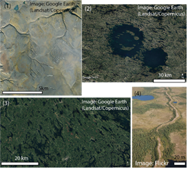
Figure 1. Fingerprints of terrestrial warm-based glaciation. (1) Subglacial channels (Nunavut). (2) Mega-scale lineations (Québec). (2) Scouring marks and striae (Finland). (4) Esker (66.1N, 104.50W).
To make progress, we use models of terrestrial glacial hydrology to interrogate how the Martian surface gravity modifies glacial drainage, ice sliding velocity, and glacial erosion rates. Taking as reference the geometry of the ancient southern circumpolar ice sheet (ASCIS) associated with the DAf [6], we model the behavior of identical ice sheets on Mars and Earth. We show that, whereas Earth’s largely inefficient glacial drainage produces glacially scoured landscapes, the lower gravity favors the formation of subglacial channelized drainage on Mars. The lack of martian glacial sliding landforms, including grooves, drumlins, lineations, etc., could then be explained. Terrestrial analogue landscapes in the Canadian Arctic (Figure 1, panel 1) further showcase the role of glacial hydrology in landscape evolution. The presence of subglacial meltwater even after the early Mars period has important implications for the history of climate, hydrology, and presence of habitable environments.
Methods: We use the terrestrial glacial hydrology framework [9,10,11] to interrogate subglacial drainage on Earth and Mars (figure 2), using an ice sheet parametrized after the ASCIS [6]. We then evaluate glacial sliding rates on Mars and Earth, for identical ice sheet geometries, by coupling glacial drainage with a model of glacial sliding [9,10].
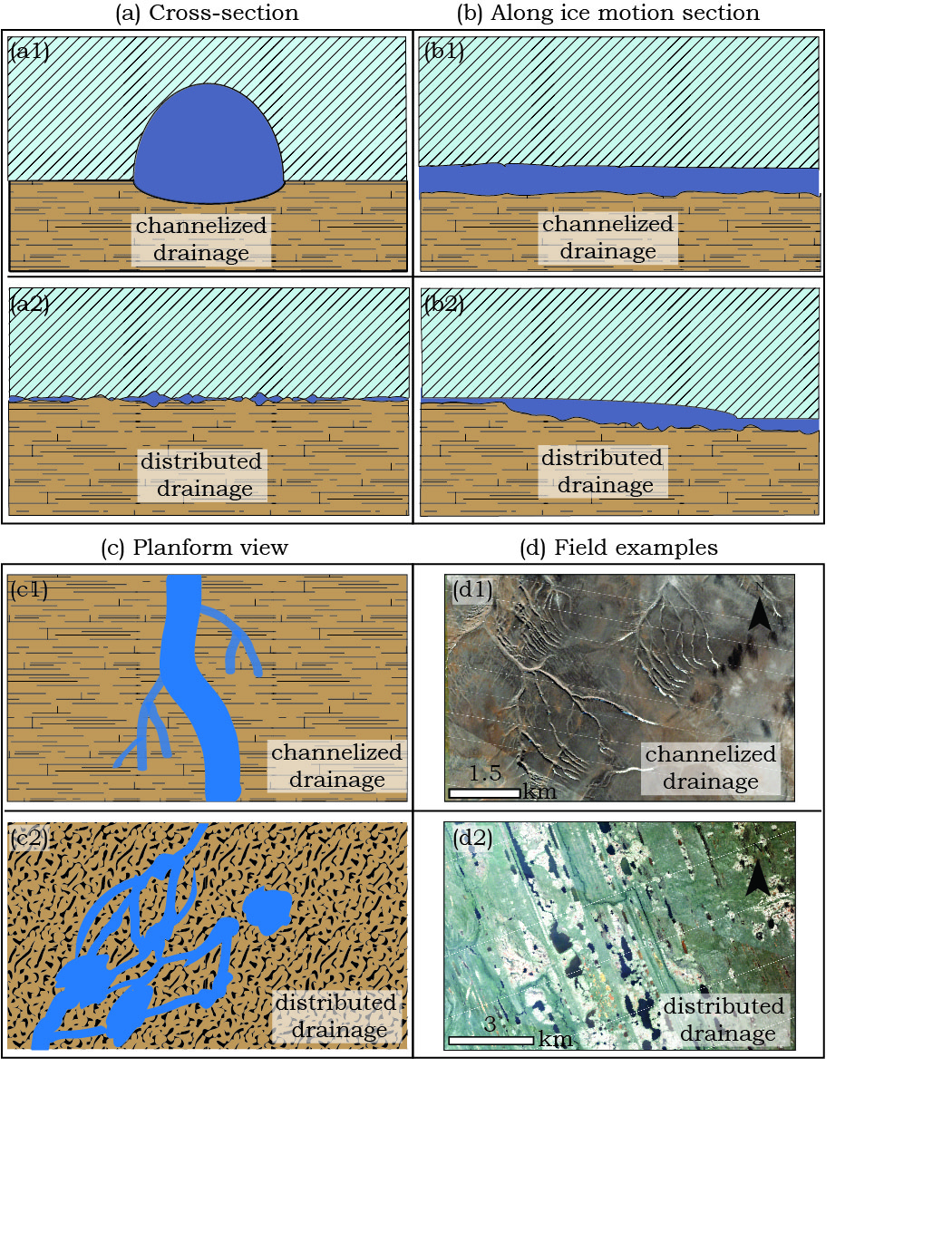
Fig. 2. Glacial drainage scenarios. Upper a,b,c panels show subglacial channels and efficient basal drainage, and their landscape expression (d). Bottom a,b,c panels show inefficient, distributed drainage by cavities, and their landscape expression (d).
When no efficient subglacial drainage exists, basal water accumulates in cavities where water pressure builds up, decreasing basal friction and accelerating ice (Figure 2) [9]. Glacial sliding then leads to highly directional, scoured landscapes (Figure 1). The opposite occurs when basal meltwater drains efficiently through subglacial channel networks [10]. Water pressure drops, basal friction increases, and ice sliding slows down. The fingerprints of channelized drainage are incised subglacial channels intertwined with depositional landforms such as eskers [12].
The feedback that defines sliding velocity as a function of effective pressure (ice overburden minus basal water pressure) and subglacial drainage efficiency (cavities/ channels) is controlled by a competition between sliding velocity and drainage system evolution [9,10,11].
Results: Figure 3 shows our results [13]. Comparing Earth and Mars curves, we notice that sliding rates are a factor ~20-90 slower for an ice sheet of the same characteristics on Mars, when the effects of glacial hydrology and drainage are considered. We also find that whereas Earth’s gravity favors less efficient drainage, subglacial drainage on Mars is dominated by channels to much larger subglacial conduit cross-section (compare arrows).
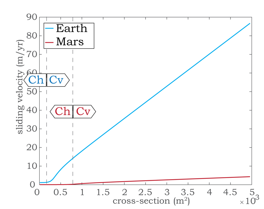
Figure 3: Results showing glacial sliding rates on Earth (blue line) and Mars (red line) vs. subglacial drainage cross-section. Cv arrows indicate the point where cavities open, Ch where channels open.
Discussion: Glacial erosion scales with ice sliding velocity to a power 1-2, so that erosion rates on Mars could be up to ~102-104 smaller than Earth according to our results. Erosion under warm-based ice masses would thus occur in channels on Mars, leading to glacial landscapes similar to those of the high Arctic (Figure 1) [12,13,14].
Conclusions: To understand the lack of martian warm-based glacial landforms we use the terrestrial glacial hydrology theoretical framework. We show that martian glacial sliding is comparatively inhibited (20-90X slower), and that glacial drainage should be dominated by channels. Hence, we infer that the fingerprints of warm-based glaciation are different between Mars and Earth, with the former being characterized by subglacial channels and eskers and the later by areal scouring by glacial sliding. This work supports the possibility that some valley networks may have formed beneath ice sheets [14], explaining the lack of warm-based glacial erosion in the Martian highlands [15] and in the Dorsa Argentea formation [5,6,7].
References:
[1] Wordsworth R. (2016) Ann. Rev. EPS 44, 381-408. [2] Kargel et al. (1995) JGR : Planets 100(E3), 5351-5368. [3] Carr M. (1995) JGR: Planets, 100(E4) 7479-7507. [4] Hynek B. et al. (2010) JGR: Planets, 115(E9). [5] Head J.W. and Pratt S. (2001) JGR: Planets, 106(E6), 12275-12299. [6] Fastook et al. (2012) Icarus, 219(1), 25-40. [7] Butcher, F.E.G. et al. (2016) Icarus, 275, 65-84. [8] Butcher et al. (2017) JGR: Planets, 122(12). 2445-2468. [9] Schoof, C. (2005) PNAS A. 461(2055), 609-627. [10] Schoof, C. (2010) Nature, 468(7325), 803. [11] Cuffey, K. M., and Paterson, W. S. B. (2010). The physics of glaciers. Academic Press. [12] Grau Galofre, A. et al. (2018), TC, 12(4), 1461. [13] Grau Galofre et al., In review. [14] Grau Galofre et al. (2020) Nat. Geosci. 13(10), 663-668. [15] Fastook, J. L., and Head, J. W. (2015). PSS, 106, 82-98.
How to cite: Grau Galofre, A., Whipple, K., Christensen, P., and Conway, S.: The record of warm-based glaciation on ancient Mars, Europlanet Science Congress 2022, Granada, Spain, 18–23 Sep 2022, EPSC2022-442, https://doi.org/10.5194/epsc2022-442, 2022.
Introduction: Glacier-like landforms (GLFs) and other classes of viscous flow features [e.g., 1-4] record the conditions when the obliquity of Mars allowed for the atmospheric deposition of ice in the mid-latitudes of Mars. However, they persist to this day because they are covered by a substantial dust that protects them from intense ablation. While substantial work has been carried out over the years to better understand and characterize GLFs, their geologic settings, morphometry, and overall morphology, we still need to better understand how GLFs evolve with time and what are the geologic or climatic controls on that evolution. Here, a preliminary comparative analysis is carried out between two notable GLF systems on opposite hemispheres: a notable mountain glacier system in eastern Argyre [5], and the central peak of Moreux crater that straddles the dichotomy boundary, and has received considerable attention given its inferred long-term glacial evolution, and potential polyphase glacial and periglacial features [e.g. 6-8]. Both systems are somewhat similar in terms of geologic setting (flows and features associated with a centralized high ground), overall scale, and apparently young age (100s of millions of years old), so a comparison of these two systems may yield new insights into how such systems evolve with time.
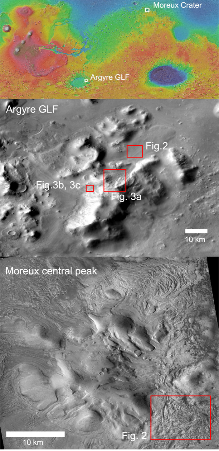
Fig 1. Top: a partly global map of Mars with superposed MOLA elevations showing the locations of the two study sites. Middle, and bottom: CTX view of the GLF in eastern Argyre and the central peak of Moreux’s Crater.
Moreux crater and its central peak: Moreux crater (41.8°N, 44.5°E) is ~133x135 km-wide complex crater, straddling the unconformity. Its northern-southern walls are more subdued and roughly the same height of the central peak, which is ~2 km high with respect to the crater floor. The central peak displays various glacial landforms and surface textures (Fig. 1). [7] indicate that the central peak has been substantially modified into an array of mounds and blocks that house coalesced flows, tributary Piedmont-like debris covered glaciers, LVF lobes, and draped flows. Furthermore, there is evidence for the development of more recent erosional features. In particular, polygonal patterns interpreted as seasonal thermal contraction cracks are observed in areas surrounding the central peak and the crater overall, as well as the areas around it [7,8]. The evidence for substantial erosion in addition to other features such as valley networks, esker-like ridges, and possible periglacial features in and around the crater suggest polyphase glacial and periglacial processes have affected the region [6-8].
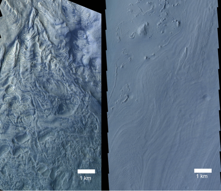
Fig 2. CaSSIS false-color composite views of parts of the GLF systems in Moreux (left) and Argyre (right). Note the clear differences in surface texture and morphological diversity between both units.
Mountain glacier system in Argyre: The glacier system (47.5°S, 326.9°E) is located along the inner eastern rim of Argyre basin, It displays a wide mesa-like flat top more than 20 km across along its longest axis with steep (22–30°) sides that have developed into cirque-like alcoves [5]. The mountain displays 3 distinct lobes that appear to flow from the base of the cirques trending NE, NW, and SW, among other flows. Similarly to Moreux, the glacier system displays multi piedmont-like terminal lobes, gullies associated with cirque-like source regions, and evidence of periglacial modification of surface materials mainly in the form of polygonally patterned grounds [5]. Finally, the Argyre system is on average 2500 m higher than Moreux, which could have an important role in how both systems evolve.
Preliminary insights: The GLF system in Moreux appears to have been substantially ablated and there is a higher diversity and a wider extent of erosional features, most notably in Fig. 2 comparing two areas of equivalent setting and at the same scale using images from the Color and Stereo Surface Imagine System (CaSSIS) [9]. The Argyre system, which appears more pristine, lack evidence for wet-based glaciation. In particular, no substantial ablation is apparent, and there is no evidence of channels or eskers in close proximity to the GLF system there. However, Argyre’s GLF, displays evidence for more substantial gully activity (Fig. 3A), which has not been unambiguously identified at Moreux’s central peak [7]. If the gullies, are carved by liquid water, then it is not apparent why gullies would be active and abundant in Argyre, but not in Moreux, which would lend support to other mechanisms not involving liquid water activity [10]. Both GLFs display evidence for recent erosional modification, and possible as evident from the presence of patterned grounds. However, in Argyre’s case, there is additional evidence of further modification postdating gullies (Fig. 3B), and localized ablation occurring preferentially at the polygonal cracks perpendicular to the local slope (Fig. 3C). In summary, there is evidence for substantial morphological differences and varied evolutionary pathways for both GLF systems inspected, and it is worth investigating the reasons for this variety. It is expected that wet-based glaciation would lead to more intense landscape modification, but it is not clear why such conditions would have existed in Moreux but not in Eastern Argyre. Further analysis is envisioned and should hopefully yield more insights.
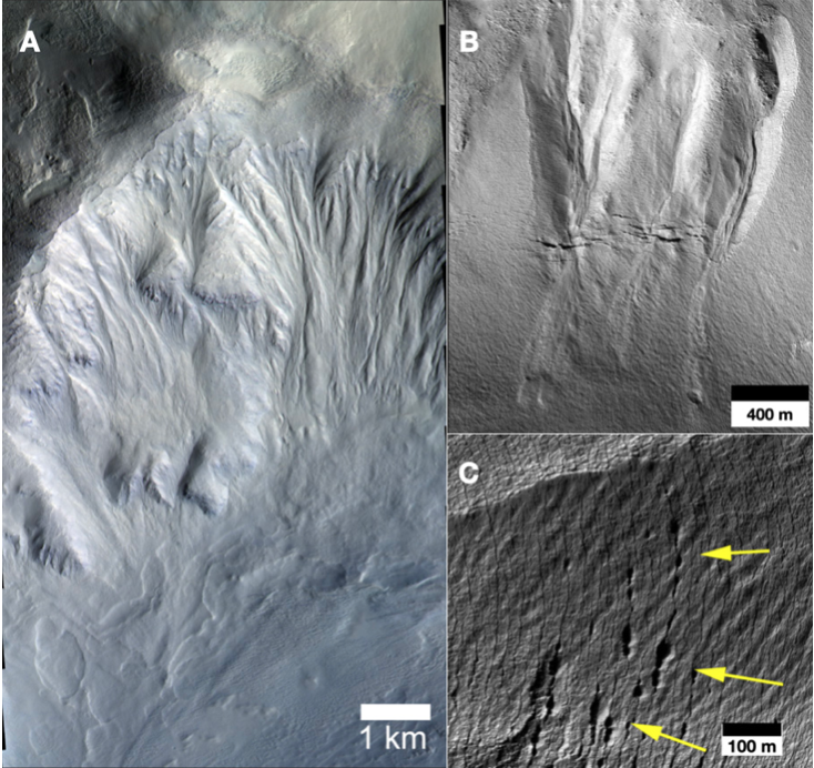
Fig 3. [A] CaSSIS false-color composite views of parts of the GLF system in Argyre showing extensive gully systems at the accumulation zone. [B] HiRISE view of the Argyre GLF showing gullies dissected by fractures. [C] HiRISE view of the Argyre GLF showing thermal contraction polygons showing progressive modification possibly caused by localized ablation along the fractured margins.
Acknowledgements: The authors acknowledge support from the internal grant 8474000336-KU-SPSC.
References: [1] Arfstrom, J., and Hartmann, W.K., (2005), Icarus, 174, 321–335. [2] Head. J.W. et al. (2010), EPSL, 294, 306–320. [3] Souness, C. et al. (2012). Icarus, 217, 243–255. [4] Hubbard, B. et al. (2014), Cryosphere, 8, 2047–2061. [5] El-Maarry M.R. and Diot, X. (2020), LPSC abstract #3070. [6] Marchant, D et al. (2006), LPSC abstract #1425. [7] Sinha R.K., and Murty S.V.S (2015), Icarus 245, 122-144. [8] Soare, R.J. et al. (2021). Icarus 362, 114401. [9] Thomas, N., et al. (2017), SSR 212, 1897-1944. [10] Dundas, C., et al. (2015), Icarus 251, 244-263.
How to cite: El-Maarry, M. R. and Harrington, E.: The glacial landscape in Moreux crater versus a mountain glacier in Argyre, Mars: A comparative analysis, Europlanet Science Congress 2022, Granada, Spain, 18–23 Sep 2022, EPSC2022-1033, https://doi.org/10.5194/epsc2022-1033, 2022.
Introduction
Apart from the Earth, no planetary body is mapped more extensively and to such fine resolution as Mars. The increasing volume of remote sensing data means we are better equipped than ever to answer the fundamental questions about the history of the planet. However, the volume of data grows much faster than the number of scientists who can use it. Machine Learning (ML) is a powerful tool for automating the analysis of ever-increasing volumes of remote sensing data.
Aeolian bedforms exhibit varied morphologies at different scales in remote sensing imagery, therefore, automated detection is a complicated problem. Linear dune fields have been successfully characterized at regional scales using edge detection on Titan from synthetic aperture radar images [1]. Within the field of Earth observation, an edge detection algorithm has been proposed that is optimized for recognizing linear dune fields in panchromatic Landsat 8 data and digital elevation models [2]. Fingerprint minutiae extraction software designed for forensic applications has also successfully detected dune crests and their bifurcations and terminations for linear dunes in the Namib Sand Sea and Strzelecki Desert, and for Transverse Aeolian Ridges (TARs) on Mars [3].
A method for mapping aeolian ripples has been demonstrated using HiRISE imagery from Gale crater [4]. Similarly to earlier studies, this uses a two-step algorithm that segments the bedforms from the surrounding terrain and then detects the crestlines [5]. This study uses the same approach but with a segmentation step that classifies bedforms according to scale and morphology as opposed to foreground-background.
The aim of this study is to create a more general bedform detector that can be applied over larger and more texturally diverse areas of Mars. Moreover, it should perform as well as classic methods employed by geologists such as manually mapping crestlines. This will be assessed in terms of orientations and crest line maps produced but also in terms of the inferred wind regime. The secondary goal of this study is to demonstrate how ML terrain classifications designed for rover navigation can be repurposed for science.
Method
A machine learning system called the Novelty or Anomaly Hunter – HiRISE (NOAH-H) has been developed to classify terrain in HiRISE images from Oxia Planum and Mawrth Vallis according to texture. It was designed to assess terrain for rover traversability but also demonstrates great potential to be used for science [6]. Each pixel of an input HiRISE image is assigned one of 14 classes. These classes represent every type of terrain that can be found at the Oxia Planum and Mawrth Vallis landing sites, summarized in table 1. Classes 8 through to 13 are the six types of ripple morphology that are recognized by NOAH-H.
| 1 | Non-bedrock | Smooth, Featureless |
| 2 | Smooth, Lineated | |
| 3 | Textured | |
| 4 | Bedrock | Smooth |
| 5 | Textured | |
| 6 | Rugged | |
| 7 | Fractured | |
| 8 | Large Ripples | Simple form, Continuous |
| 9 | Simple form, Isolated | |
| 10 | Rectilinear form | |
| 11 | Small Ripples | Continuous |
| 12 | Non-continuous, Bedrock substrate | |
| 13 | Non-continuous, Non-bedrock substrate | |
| 14 | Other Cover | Boulder fields |
Table 1: Ontological classes used by NOAH-H. Large refers to decimeter scale features and small refers to meter scale features.
Class 9, "large simple form isolated ripples", corresponds to the larger-scale TARs in these regions and we use the NOAH-H output to segment the TARs from the surrounding terrain. Some of these classified regions contain more than one TAR, therefore the next step splits these into separate regions. Now that we can assume that every region corresponds to a single TAR, we calculate an orientation for each region using second order central image moments.
Planned Analysis
This method will be applied to HiRISE images already classified by NOAH-H in Oxia Planum. We will compare the spatial distribution and orientation of TARs using the proposed method with those measured from a study that measured 10,753 TARs by manually digitizing crestlines [8]. They will also be compared in terms of inferred wind regime and compared with a global climate model to see if they give the same conclusions. The next step to build on this work is to implement existing or new methods for the remaining 5 bedform classes detectable by NOAH-H, in order to make a more general bedform characterization method.
References: [1] Lucas A. et al. (2014) JGR, 41, 6093–6100. [2] Telfer M. W. et al. (2015) Aeolian Research, 19, 215-224. [3] Scuderi L. (2019) Aeolian Research, 39, 1-12. [4] Vaz D. A. and Silvestro S. (2014) Icarus, 230, 151-161. [5] Pina P. et al. (2004) LPS XXXV, Abstract #1621. [6] Barrett A. M. et al. (2022) Icarus, 371, 114701. [7] Canny J. (1986) IEEE TPAMI, PAMI-8, 6, 679-698. [8] Favaro E. A. et al. (2021) JGR Planets, 126, e2020JE006723.
How to cite: Bohacek, E., Barrett, A., Favaro, E., Balme, M., and Sefton-Nash, E.: Transverse Aeolian Ridges at the ExoMars Rover landing sites, Europlanet Science Congress 2022, Granada, Spain, 18–23 Sep 2022, EPSC2022-957, https://doi.org/10.5194/epsc2022-957, 2022.
Introduction: Louth Crater is a 36 km diameter located at 70 °N, 103.2 °E (Fig. 1) less than 1000 km from the Martian North Polar Cap. At the center of Louth crater a perennial water ice cap ~10 km in diameter, ~250 m in width (Fig. 1) that undergoes phase changes (condensation / sublimation cycles) during the Martian year [1 - 4]. Some periodic structure at the surface of its perennial water ice cap have been observed [2]. The presence of smaller ice undulations superimposed on this periodic structure, comparable to the sublimation waves on the Martian North Polar Cap [5] could be formed during sublimation and condensation period of the water ice. The characterization of this ice waves could make it possible to specify environmental conditions favorable to their formation. The first part of the study consists of identifying these ice waves using orbital topography and imaging data, and then associating these results with data from the Martian Database [6-7] and with the scaling laws inherent to the formation of sublimation and condensation waves.
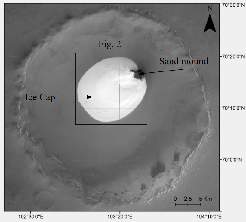
Fig. 1: Louth crater in summer. CTX product J02_045439_2504_XN_70N256W Ls = 133.2°
Geomorphological analysis:
Methods: Digital Elevation Model (DEM) at ~100 m/pixel and MOLA elevation data at ~128 m/pixel have been coupled with imagery data from HRSC ~10 m/pixel, CTX at ~6 m/pixel and HiRISE images for more precise areas for up to 25 cm/pixel. Data were georeferenced in ESRI’s ArcMap GIS software to produce geomorphological map and analyzed to evaluate ice waves shape and spatial organization.
Observations: Louth presents two units (Fig. 2). (a) Lower unit with dark stucco texture and stratifications (Fig. 3a). (b) Fresh ice overlies this older, stratified structure (Fig 3.a). This fresh ice is distributed in a non-uniform manner as shown by the kilometrics waves of about 560 m wavelength on which are superimposed decametrics waves of about 55 m wavelength which are both perpendicular to the prevailing wind (Fig 3.b). The crests of both wave populations show similar NW-SE. The main wind direction was assessed from barkhane field on the sand mound.
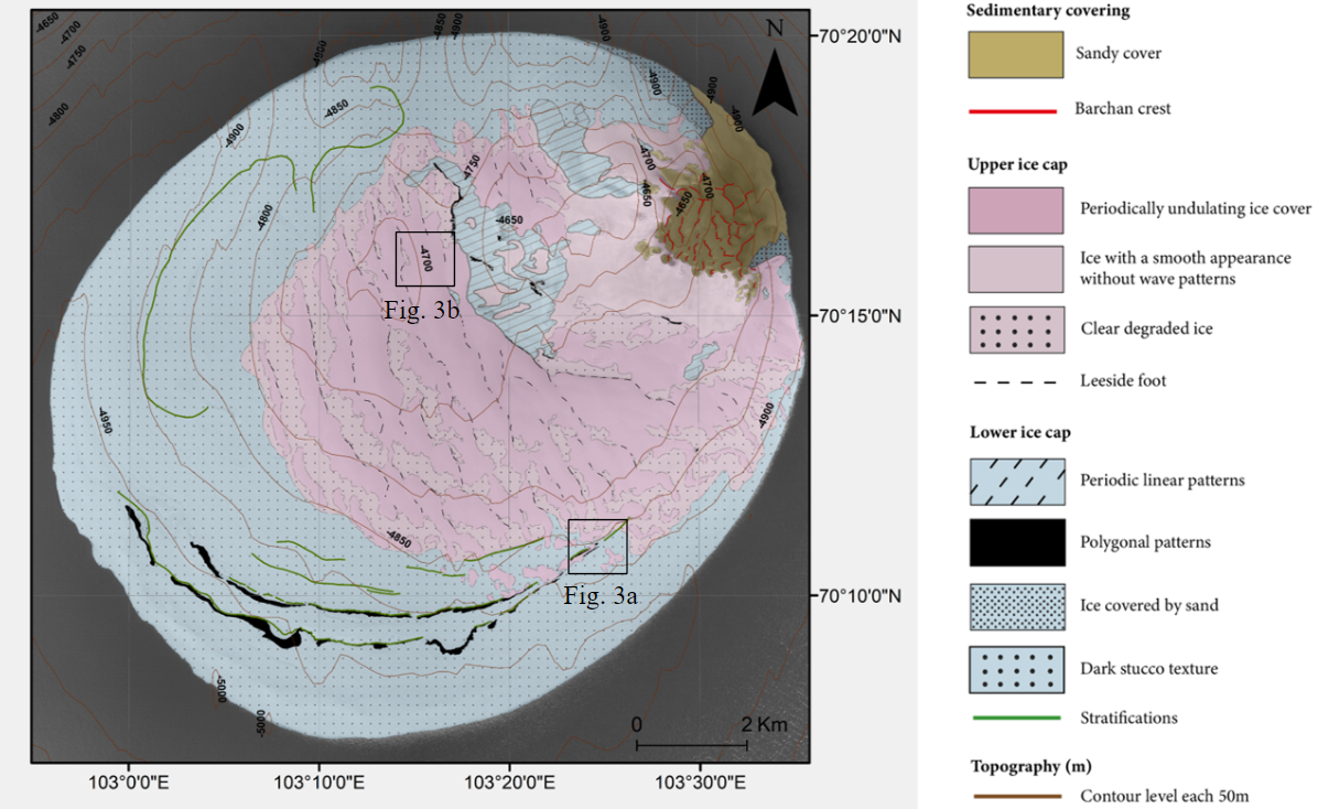
Fig. 2: Louth’s geomorphological map in summer. CTX product J02_045439_2504_XN_70N256W Ls = 133.2°.
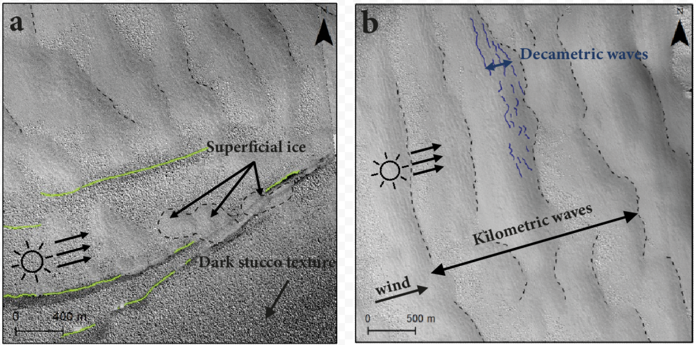
Fig. 3: Boxes from Fig. 2. (a) East side of the Louth crater ice cap. Green lines represents stratifications, HiRISE product EPS_045439_2505, Ls = 133.2°. (b) decametric waves on the ice waves. Black dashes represent leeside foot of each kilometric waves. Blue lines emphasize decametric waves, same HiRISE product from (a).
Transport hypothesis: Preliminary experiments studied the threshold velocity necessary to initiate a transport of ice grains in Martian Simulation Wind Tunnel [8]. These experiments were carried out for grains from a few hundred micrometers to 2 mm in diameter under atmospheric pressures of 40 to 1000 mbar. To transport ice particles under near-Martian condition is hard because the threshold velocity is ten times higher than Earth. The wind speeds estimated from the Martian Database [6-7] in Louth crater are much lower than those needed to transport ice grains at Martian pressure. We support the hypothesis of diffusion by sublimation/condensation rather than the transport of icy particles by the wind.
Mass transfer hypothesis: In a recent theoretical model [5] scaling laws explain the formation of sublimation waves and have been validated on terrestrial bedforms and on the Martian North Polar Cap. These waves are periodic and oriented in accordance with a turbulent boundary layer flow that diffuse the sublimated vapor. These laws, which are superimposed on the two ice waves studied, make these waves suitable geomorphological markers for climatic predictions. This model has been adapted to study similar waves created by condensation [9] and results indicate that condensation waves would be larger with one order gap than sublimation waves.
Discussion: From the wind tunnel experimentation of ice particles transport in Martian-Like environment [8], wind necessary to initiate transport of ice particles is unlikely in Louth. Friction velocities of 3 m.s-1 would be required, compared to 0.6 m.s-1 deduced from scaling laws, to transport the most mobilizable 0.3 mm ice particles [8]. Wind speed in Louth is too weak for initiating particles transport. From the scaling laws, we extract values of friction velocity and flow velocity at a given altitude that can be compared with those extracted from the Martian Data Base over two Martian periods: a period of sublimation (during the summer in the northern hemisphere) at the origin of the formation of decametric waves and a period of condensation at the end of the summer, beginning of the autumn favorable for the kilometric waves formation. Scaling laws are in agreement with the predicted ratio velocity between sublimation and condensation period from the Martian Data Base values. From the Martian Data Base, independent velocity values are larger. This can be explained by the gridding of the database which takes place on a global scale larger than the crater.
Conclusion: The observations indicate kilometric bedforms on the ice cap of Louth Crater, on which decametric bedforms appear with an order of magnitude gap. Comparison with numerical results suggests that the kilometric bedforms are formed by condensation and the smaller ones by sublimation. These condensation and sublimation waves are suitable markers to constrain mesoscale climate modelling in small, complex regions such as this type of crater, where topographic and/or seasonal effects can affect climate data. These waves can also be used as geomarkers on other planetary bodies where climatic conditions are not well constrained.
Acknowledgments: We acknowledge PNP (Plan National de Planétologie) for founding the project “sublimation and condensation waves”. We used Planetary Data System (PDS) for observational data.
References: [1] Conway et al. (2012) Icarus. [2] Brown et al. (2008) Icarus. [3] Hofstader & Murray (1990) Icarus. [4] Appéré et al. (2011) Journal of Geophysical Research. [5] Bordiec M. et al. (2020) Earth-Science Reviews, 211, 103350.[6] Forget et al. (1999). [7] Millour et al. (2018). [8] Herny et al. (2020). 7th Mars Polar Science Conf. Abstract #2099. [9] Carpy S. et al. (2022). EGU, Abstract #5998.
How to cite: Collet, A., Carpy, S., Bordiec, M., Massé, M., Bourgeois, O., and Conway, S.: Aeolian bedforms formed by ice sublimation and vapor condensation on Louth crater ice, Mars., Europlanet Science Congress 2022, Granada, Spain, 18–23 Sep 2022, EPSC2022-471, https://doi.org/10.5194/epsc2022-471, 2022.
Please decide on your access
Please use the buttons below to download the presentation materials or to visit the external website where the presentation is linked. Regarding the external link, please note that Copernicus Meetings cannot accept any liability for the content and the website you will visit.
Forward to presentation link
You are going to open an external link to the presentation as indicated by the authors. Copernicus Meetings cannot accept any liability for the content and the website you will visit.
We are sorry, but presentations are only available for users who registered for the conference. Thank you.
Posters: Thu, 22 Sep, 18:45–20:15 | Poster area Level 1
Introduction. ExoMars rover mission is planned to deliver the ‘Rosalind Franklin’ rover to explore Oxia Planum, a region that straddles between Arabia Terra and Chryse Planitia (335.5E, 18.2N). Oxia Planum bears several evidences of aqueous activity [1-4], where infrared data reveal extensive outcrops of recently exhumed clay-rich rocks. These outcrops are perfect “windows” to search for signs of past or present life on Mars, as biosignatures might be preserved therein [5]. Clays detected at Oxia Planum are among those found all over circum-Chryse Planitia [6], a flat lowland region and bottom end of many outflow channels.
Here, we focus on possible clay-bearing outcrops detected in northern Xanthe Terra (313E, 13N) (Figure 1), a region that has already been suggested for several rover missions. Like in Oxia Planum, several morphological features advocate for a fluvio-deltaic and lacustrine history in the region [7-9], with fluvial channels and fan deltas (e.g., Sabrina and Hypanis valley systems). Despite a possible detection of Fe,Mg-rich clays at the Sabrina delta [10,11], no detailed spectral survey have been done in the entire area. A detailed analysis of these outcrops is crucial to better determine possible mineral phase(s) and search for changes in clay mineralogies associated with differences in formation and weathering conditions. We examine infrared data, particularly the absorptions centered in the 1.0–2.6 μm spectral range, in order to better constrain the nature and composition of the clays.

Figure 1 – Locations of Oxia Planum (OP) and northern Xanthe Terra (XT) at the margins of circum-Chryse Planitia.
Data & Methods. Spectral signatures of the clay outcrops are obtained from data gathered by the CRISM instrument, with spatial resolutions of 20–40 m.px-1 and a spectral resolution of 6.6 nm [12]. For this study we use several CRISM cubes acquired in the near-infrared spectral range (1–4 µm), targeting the northern Xanthe Terra. They are first pre-processed through CAT ENVI for atmospheric and photometric corrections. Corrected cubes are then denoised (column-by-column ratio) to reduce noise and residual atmospheric contributions, and to finally emphasize mineralogical absorptions in the ratioed spectrum. Once the cubes are corrected and denoised, we define our regions of interest (ROIs) to outline clays. We calculate band depths at 1.9 and 2.3 µm [13] to select pixels with strong absorptions and map the ROIs for each cube (Figure 2).

Figure 2 – Two sites of interest exposing clay-bearing outcrops: near the Sabrina fan delta at the Magong crater (313.4E, 12.1N) and an isolated outcrop in eastern Xanthe Terra (317.5E, 10N). We also include the possible clay outcrops identified at the delta [10,11].
Results. For each cube, we retrieve the band centers for all pixel of the ROIs within the three spectral ranges of interest: 1.4 µm (1.37–1.45), 1.9 µm (1.88–1.96), and 2.3 µm (2.26–2.34) (after continuum removal to emphasize the absorptions). The band centers do not strongly vary for the three narrow absorptions, with average values being 1.408 ± 0.009 µm, 1.923 ± 0.008 µm, and 2.305 ± 0.009 µm. FRT0A605 is the only cube displaying a clear overtone near 2.4 µm and a shallow absorption near 2.5 µm. We therefore retrieve the band centers near 2.4 µm (2.36–2.44) and 2.5 µm (2.49–2.57), where the cube shows average values of 2.397 ± 0.009 µm, and 2.530 ± 0.010 µm. Overall, these values are identical to those recently obtained at Oxia Planum [4] (Figure 3).

Figure 3 – (left) Spectra of CRISM denoised reflectance (normalized and offset for clarity) obtained in northern Xanthe Terra. (top right) We also include three spectra from Oxia Planum [4]. (bottom right) Lab spectra of main candidate Fe,Mg-rich clays (RELAB).
Discussion. CRISM cubes reveal several absorptions in the 1.1–2.6 µm range. Absorptions near 1.4 and 1.9 µm are common to hydrated minerals (OH/H2O stretching), while an absorption near 2.3 µm indicates a (Fe,Mg)-OH vibration. Xanthe’s clays are consistent with Fe,Mg-rich clays, combining absorptions at 1.41, 1.92, 2.30–2.31 µm and weaker overtones near 2.39–2.40 µm. Martian Fe,Mg-rich clays generally show spectral variability in the three windows. Xanthe’s clays intermediate band centers are consistent with either vermiculites and Fe-rich saponite (Figure 3), like in Oxia [4]. Band centers within these windows vary very little throughout the region. Exact positions therein depend on the relative abundance of iron and magnesium in the clay structure, and also oxidation state of iron.
Conclusions. We provide in-depth information on the clay-bearing outcrops found in northern Xanthe Terra, to compare with recent results obtained in Oxia Planum [2,4]: (1) report exact positions of the 1.4, 1.9, 2.3, 2.4 and 2.5 µm absorption bands, and (2) map the “purest” clays in the targeted areas, in context with the morphology and topography. This allows for further investigations in context with the ExoMars rover mission or other future rover missions.
Acknowledgments. This work is fully funded and supported by the Italian Space Agency (ASI) [Grant ASI-INAF n. 2017-48-H.0]. We are greatly thankful to the CRISM team for the CAT tool, and European Space Agency (ESA) and Russian Space Agency ROSCOSMOS for the ExoMars project.
References. [1] Carter et al. (2016) 47th LPSC Abstracts, 2064. [2] Mandon et al. (2021) Astrobiology 21, 464–480. [3] Quantin-Nataf et al. (2021) Astrobiology 21, 345–366. [4] Brossier et al. (under review) Icarus. [5] Vago et al. (2017) Astrobiology 17, 471–510. [6] Carter et al. (2013) JGR 118, 831–858. [7] Fawdon et al. (2018) EPSL 500, 225–241. [8] Adler et al. (2019) Icarus 319, 885–908. [9] Adler et al. (2022) JGR 127, e2021JE006994. [10] Platz et al. (2014) 9th EPSC Abstracts, 811. [11] Knade et al. (2017) 11th EPSC Abstracts, 692-1. [12] Murchie et al. (2007) JGR 112, E05S03; Murchie et al. (2009) JGR 114, E00D07. [13] Viviano-Beck et al. (2014) JGR 119, 1403–1431. [14] Ehlmann et al. (2008) Science 322, 1828–1832.
How to cite: Brossier, J., Altieri, F., De Sanctis, M. C., Frigeri, A., Ferrari, M., Apuzzo, A., and Costa, N.: Spectral Survey on Clay-rich Outcrops in Northern Xanthe Terra, Reference Sites for Oxia Planum, Europlanet Science Congress 2022, Granada, Spain, 18–23 Sep 2022, EPSC2022-12, https://doi.org/10.5194/epsc2022-12, 2022.
MarsSI (“Mars Système d’Information”, french for Mars Information System) is a platform and service to explore, process and retrieve data from orbiters. https://marssi.univ-lyon1.fr/MarsSI. This poster aim to help user to understand and use this service.
Introduction
Geological investigations of planetary surfaces require the combination of orbital datasets. Missions being often multiple-instruments platforms from multiple space agencies, the quantity of data available increased quickly. MarsSI is a platform designed to explore, process and retrieve Mars orbital data. It was certified in 2017 as french national Research Infrastructure by the Centre National de la Recherche Scientifique (CNRS) as part of the Planetary Surface Portal (PSUP, <https://psup.cnrs.fr/>).
As of 2021, it indexes the optical (visible, multi and hyper-spectral) data from the recent orbiter missions, and allow to request the creation of Digital Elevation Models on demand. The focus, as highlighted by figure 1 is to allow the user to browse and request ”ready-to-use” products in regards of calibration, refinements and georeferencing. The user will be able to visualize and interpret the data in GIS or remote sensing software.
MarsSI
MarsSI aim to provide both a way to explore and use data from space agencies archives, such as the Planetary Data System (PDS), but also run data processing pipelines to make this data ready for analysis and as a shared, collaborative, repository. This allows a scientific user to more easily access data from their raw level and proceed to surface investigations and interpretation.
Explore datasets
MarsSI access is done through a web application. This interface, completely updated in 2021, provide a map where product footprints can be visualized over various backgrounds (MOLA, Themis, CTX) to put data in context. Instruments, and if needed, their acquisition modes, are available as layers to display.
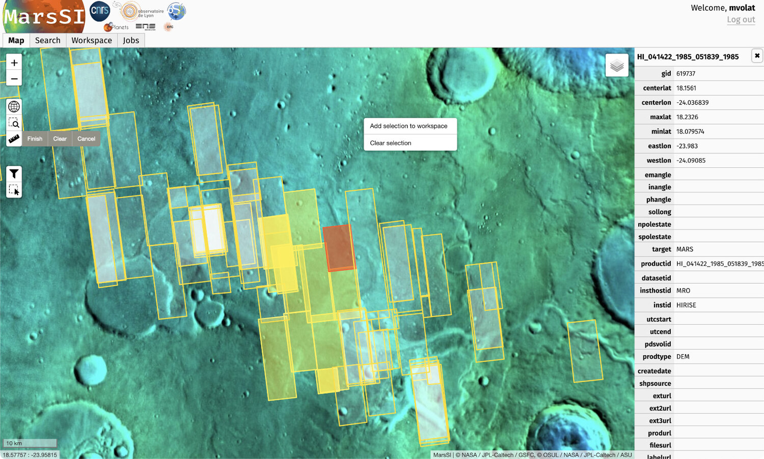
In this part of the interface, the user will be able to select products of interest and add them to a workspace summarizing the data he need to use.
Until now, MarsSI has focused on the most recent missions (ODY, MEX, MRO) optical datasets (visible, NIR, hyperspectral) and derived products.
Pipelines
Pipelines execution is done on demand, and requested from the workspace pane of the interface. Each type of product (based on instrument) has a specific pipeline defined. The pipelines are designed to be fully automated, run on MarsSI's computing cluster, and to not require any user input. This is done partially to ease the usage of the service, to avoid managing and storing multiple versions with slight differences that would make references to products more complex.
Basic pipelines operate to bring products to calibration and map projection (and georeferencing) steps. Those pipelines are usually based on ISIS (https://isis.astrogeology.usgs.gov/) for visible spectrum images.
More advanced pipelines allows to calibrate and create spectral parameter maps from CRISM hyperspectral cubes using the CRISM Analysis Toolkit (CAT, https://pds-geosciences.wustl.edu/missions/mro/crism.htm), and another to create stereophotogrammetry-derived DEMs from the CTX and HiRISE datasets (in complement of the pre-processed DEM datasets available) based on Ames StereoPipeline (https://ti.arc.nasa.gov/tech/asr/groups/intelligent-robotics/ngt/stereo/). One notable feature is that the DEM datasets are computed from the optical imagery datasets, showing all the stereo pairs deemed feasibles (based on overlap calculation and having a difference of incidence angle of at least 10°).
Documentation
MarsSI is documented through a wiki that provide information on both the platform usage and the products.
Conclusion
MarsSI (https://marssi.univ-lyon1.fr) aims to offer a way to the scientific communities to easily explore and perform the necessary processing steps for the data needed in their projects. MarsSI itself has seen superficial and architectural changes since it was recognized as part of a french national service, and aim to extend its datasets range in the future. Use of the service require registration that is free for a non-commercial usage.
Ackowledgements
MarsSI is a national Research Infrastructure, recognised as such by the French Ministry of Higher Education and Research. It was supported by the Programme National de Planétologie (PNP) of CNRS/INSU, co-funded by CNES. It was initialy supported by the European Research Council under the European Union’s Seventh Framework Program (FP7/2007-2013)/ERC Grant agreement No.280168.
How to cite: Volat, M. and Quantin-Nataf, C.: MarsSI: Martian surface data processing service, Europlanet Science Congress 2022, Granada, Spain, 18–23 Sep 2022, EPSC2022-213, https://doi.org/10.5194/epsc2022-213, 2022.
Introduction: Despite the large amount of information from orbital and in situ missions, the characteristics and evolution of Mars’ early climate are still widely debated among the scientific community. Morphological evidence dating back to about 3-4 billion years ago, such as valley networks [1], and the presence of several hydrated minerals [2] seem to indicate that Mars once had a “warm and wet” climate with abundant water on the surface and possibly even an ocean in the northern lowlands [1-3]. These conditions eventually changed through time leading up to the hyperarid and cold planet we observe today.
The area of Meridiani Planum (MP), located SW of Arabia Terra, is well known for retaining multiple evidence of past aqueous activity [4] and a varied hydrated mineralogy [5]. The majority of the terrains exposed in MP formed at the Noachian-Hesperian boundary [6], that is between two important epochs of Mars: the Noachian (4.1-3.7 Ga), where most of the evidence for water is found, and the Hesperian (3.7-3.0 Ga), which is characterized by increasingly water-limited conditions. Constraining the potential water environment at the NH boundary is fundamental to understand Mars’ early climate and its evolution.
In this study, we select 7 craters in Northern MP (figure 1) showing evidence of NH sediment infillings with hydrated materials (e.g., clays and sulfates) to assess in detail the stratigraphic sequence of the mineralogical units and understand their origin and diagenetic history. The craters are roughly aligned SE to NW following the general slope of the area from the highlands to the lowlands. If Mars experienced a “warm and wet” period, MP would represent a transition zone between the subaerial alteration environment of the highlands and the subaqueous environment of the Martian ocean. Therefore, the area would be easily affected by climatic changes whose evidence should be retained in its sedimentary sequences.
We show here some preliminary results from 2 out of the 7 craters selected for the study:
1) a 15-km-wide crater named Mikumi, centered at Lat. 2.45°N, Lon. 359.96°E;
2) an 18-km-wide unnamed crater centered at Lat. 4.25°N, Lon. 2.85°E.

Figure 1: THEMIS daytime image of Meridiani Planum. Selected craters are evidenced with points. Name (if given) and coordinates of the center for each crater are also indicated with a label. Most of the craters are unnamed. The arrows indicate the two craters described in this abstract.
Datasets and methods: We investigate the mineralogy of the craters’ terrains through CRISM [7] hyperspectral data cubes mainly in the range 1.0-2.6 μm. This interval retains part of the key spectral features of primary rock-forming minerals, which constitute the Martian crust, and of most minerals produced by secondary processes such as aqueous circulation and alteration (e.g., clays and sulfates). MOLA, THEMIS, CTX and HiRISE data are then used for morpho-stratigraphy and camera imaging.
Results: Two types of clays (smectites) with different Fe/Mg content, polyhydrated sulfates and monohydrated sulfates are observed in both craters (figure 2). Fe/Mg-clay spectra (e.g., nontronite and saponite) show absorptions at around 1.4, 1.9 and 2.3 μm with additional overtones at 2.4 μm. The exact position of the 2.3 μm feature depends on the relative Fe/Mg content in the clay mineral. We find some areas with clays richer in iron (e.g., nontronite), showing this feature centered at 2.305 μm, and clays richer in magnesium (e.g., saponite) where the absorption is centered at 2.310-2.315 μm. In Mikumi crater, polyhydrated sulfates (Mg sulfate) and monohydrated sulfates (kieserite) are detected stratigraphically below the clay-bearing layer. For the unnamed crater, the stratigraphic relationship of the units is still to be investigated.
Figure 2: (top) CRISM spectra of detected mineralogy. Fe/Mg clays (smectites) are from Mikumi crater, mono and polyhydrated sulfates are from the Unnamed crater. The spectra are extracted from FRT0000BEF5 and FRT00009B5A TRR datasets respectively. (bottom) Laboratory spectra of clays and sulfates from the CRISM spectral library [8] (Mg Sulfate ID: CJB366; Kieserite ID: F1CC15; Saponite ID: LASA51; Nontronite ID: NCJB26).
Discussion and conclusions: Clays and sulfates on Mars appear to have formed at different times and under different climatic conditions [9]. Clays are usually associated to Noachian terrains and may have formed under alkaline conditions in a “warm and wet” ancient Mars, whereas sulfates are typically associated to Hesperian surfaces and may have formed under a dryer and more acidic environment. Therefore, sulfates are expected to be found stratigraphically on top of clays, as they should have formed later in Mars’ history. However, this distinction between a clay-rich Noachian and a sulfate-rich Hesperian oversimplifies the history of the aqueous chemistry and climate of Mars especially near the NH boundary.
Our analysis suggests a stratigraphic sequence with interleaving clays and sulfates at the NH boundary. Similar stratigraphic sequences have also been observed in other areas of MP (Southern MP) by [5]. In the case of [5], a clay-bearing layer is overlain by other sulfates, generating a sulfate/clay/sulfate stratigraphic sequence. All this argues is in favor of several distinct climatic episodes pacing the NH climatic transition.
The results obtained so far will be enriched by further analysis of these areas along with a thorough investigation of the remaining 5 craters selected.
Acknowledgments: Featured CRISM data were downloaded from the Planetary Data System (PDS). This project is partially supported by Europlanet RI20-24 GMAP project.
References: [1] M. H. Carr and J. W. Head (2010) Earth and Planet. Sci. Lett., 293, 185-203. [2] B. L. Ehlmann and C. S. Edwards (2014) Annu. Rev. Earth Planet. Sci., 42, 291-315. [3] R. A. Craddock and A. D. Howard (2002) JGR, 107 (E11), 5111. [4] R. M. E. Williams et al. (2017) GRL, 44, 1669-1678. [5] J. Flahaut et al. (2015) Icarus, 248, 269-288. [6] B. M. Hynek et al. (2002) JGR, 107 (E10), 5088. [7] S. Murchie et al. (2007) JGR, 112 (E5), E05S03. [8] C. E. Viviano-Beck et al. (2015) MRO CRISM Type Spectra Library, NASA Planetary Data System. https://crismtypespectra.rsl.wustl.edu [9] J. P. Bibring et al. (2006) Science, 312, 400-404.
How to cite: Baschetti, B., Massironi, M., Carli, C., Altieri, F., and Frigeri, A.: Clay and sulfate-bearing terrains in Northern Meridiani Planum, Mars: constraining the characteristics of Mars’ early climate at the Noachian-Hesperian boundary, Europlanet Science Congress 2022, Granada, Spain, 18–23 Sep 2022, EPSC2022-222, https://doi.org/10.5194/epsc2022-222, 2022.
Introduction: Martian valley networks are evidence of surface run-off and past water cycles on ancient Mars [e.g. 1–3]. It is generally agreed that most Martian valley networks formed as a result of precipitation-fed fluvial [4, 5] in Late Noachian to Early Hesperian (~ 3.7 Ga) [e.g., 3], indicating this was the period of peak fluvial activity [e.g., 4].
The chronology between the development of Martian valley networks and the establishment of the giant volcanic province, the Tharsis Rise, is still uncertain. To better understand this chronology, attention has been paid to the relationship between valley orientation and topographic slope direction [6; 7]. Hereon, this type of analysis is referred to as discordance analysis – defined as the difference between valley orientation and the surrounding topographic surface slope direction of steepest descent [8]. Generally, the orientation of precipitation-fed rivers, and the valleys they carve, are controlled by topographic slope direction. Phillips et al. [2001] concluded that the valley network orientations were controlled by Tharsis-induced slopes, implying that the valleys predominantly post-date it. In contrast, Bouley et al. [2016] found that the orientations of the valley networks are consistent with calculations of the equilibrium shape of Mars with Tharsis Rise removed, implying that they pre-date it. These studies use low-resolution maps and do not indicate the directional discrepancy of discordance. As discordance is likely to occur over short spatial scales [8; 9] and arise from a variety of factors [8; 10], detailed mapping of smaller valleys is necessary to reveal its origin.
Bahia et al., [2022] applied discordance analysis to a latitudinal strip between 20° E to 20° W (Fig. 1); this is too far from Tharsis and its associated areas of topographic modification (e.g., the antipodal high) [11] to provide information about conformity/discordance between valley networks and Tharsis induced topography (Fig. 1). If Martian valley networks predominantly incised before the formation of the Tharsis Rise the valley networks around areas of topographic change would display some level of discordance.
In this study, valleys are mapped in high-resolution around the Tharsis Rise and the antipodal high regions, to apply discordance analysis. Reviewing any potential discordance patterns that immerge, or lack thereof, may reveal insight into the chronology between the development of the Tharsis Rise and valley network incision.
Data and Methods: Valley are identified in ESA Mars Express Orbiter – High/Super Resolution Stereo Colour Imager (HRSC) images (~ 25 m per pixel) and manually mapped, in the areas of expected topographic uplift induced by the Tharsis Rise [11], using the polyline function within ArcGIS Pro, defined under analogous characteristics as those of previous studies [e.g., 3, 8].
Tharsis-induced uplift is predicted to have occurred mostly before the Mid-Hesperian [16], so valleys incising surfaces younger than this age are unlikely to have been directly affected. To determine the relative surface ages, the Tanaka et al. (2014) digital global map of Mars was used [17].
For the present-day topography, the Mars MGS MOLA DEM 463m (MOLA DEM) was used [12-14]. Conformity between valley orientation and topographic surface slope direction is scale-dependent [8; 9; 15], hence a range of DEMs (1 km, 10 km, and 50 km per pixel) were produced from the MOLA DEM.
To find areas of discordance the present-day topographic slope direction of steepest descent (θ) and valley orientations (Ψ) will be measured. The ArcMap Pro Spatial Analyst – Aspect tool, which calculates the azimuthal direction of steepest descent for each square-shaped pixel, will be used to convert the DEMs into maps of θ. Ψ will be calculated using the ArcMap Spatial Analyst - Linear Direction Mean function. θ and Ψ will be extracted every 463m and an average for each valley/tributary will be calculated. The difference between the average θ and Ψ will be calculated to give a D (discordance) value for each individual valley/tributary.
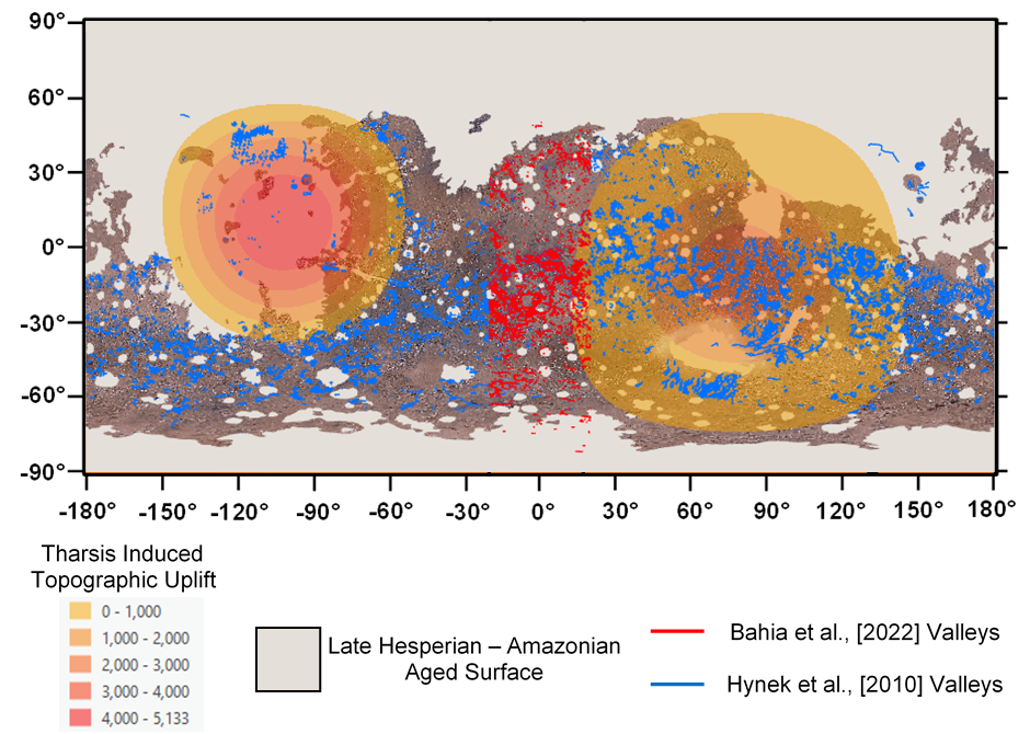
Fig. 1 Equirectangular projection of the Martian surface, showing the location of valleys mapped by Bahia et al., [2022] (red lines) using HRSC images (15 to 25 m per pixel) and Hynek et al., [2010] (blue lines) using THEMIS (Thermal Emission Imaging System) daytime and night-time IR (Infra-red) (100 m/pixel), MOC (Mars Orbital Camera) wide-angle (231 m/pixel), and MOLA (~500 m/pixel) topographic data. The grey areas are those assigned an age of Late Hesperian or younger [17]. The yellow to red shaded areas are those modeled to have experienced uplift as a result of the emplacement of the Tharsis Rise [11]. The base map is the Viking mosaic base map.
Initial Results: The cumulative area that is predicted to have experienced topographic uplift as a result of the emplacement of the Tharsis Rise [11] is around 64,770,287 km2; 36.5 % in the western hemisphere (Tharsis region) and 63.5 % in the eastern hemisphere (antipodal high). A lot of which is Late Hesperian to Amazonian in age (~ 40 %), particularly in the western hemisphere (Fig. 1), emphasizing the need to map the valleys of the antipodal high region.
At the point of abstract submission, 369 HRSC images have been mapped (~ 25,000,000 km2, ~ 40 % of the study area). In total, ~14,000 valleys have been mapped with a total valley length of ~160,000 km. On completion of this map, discordance analysis shall be performed and the discordance patterns assessed.
References: [1] Milton D. J. (1973) JGR, 78. [2] Carr M. H. (1995) JGR, 100. [3] Hynek B. M. et al. (2010) JGR, 115. [4] Kite, E. S. (2019) Space Sci Rev., 215:10. [5] Craddock R. A. and Howard A. D. (2002) JGR, 107. [6] Phillips et al., (2001) Science, 291. [7] Bouley et al., (2016) Nature, 531. [8] Bahia et al., (2022) Icarus, Accepted, 115041. [9] Black et al., (2017) Science, 356. [10] Bahia et al., (2021) LPSC 52, No. 2548. [11] Matsuyama and Manga (2010) JGR, 115. [12] Smith et al., (2001) JGR, 106. [13] Neumann et al., (2001) JGR, 106. [14] Lemoine et al., (2001) JGR, 106. [15] Lipps and Roberts (2020) Geophysical Research Letters, 48. [16] Bouley et al., (2018) EPSL, 488. [17] Tanaka et al. (2014), Planet. Space Sci., 95.
How to cite: Bahia, R.: The Chronology between the Development of the Tharsis Rise and Martian Valley Networks – A Discordance Analysis Perspective., Europlanet Science Congress 2022, Granada, Spain, 18–23 Sep 2022, EPSC2022-223, https://doi.org/10.5194/epsc2022-223, 2022.
The Curiosity rover of the Mars Science Laboratory has been exploring since mid-2021 the lower sulfate unit of Mount Sharp in the Gale crater. This unit, first described from orbital observations as showing spectral signatures of hydrated sulfate minerals [1], has recently been revealed to record a major paleoenvironmental and climatic transition during the Hesperian-Noachian transition, with the onset of alternating wet and dry conditions before a complete aridification of Martian conditions [2]. Before the current campaign, this unit was mainly studied using remote observations (e.g., [2, 3]), but Curiosity has now entered this major interval allowing to precisely study the rock record leading to this major climatic event.
Since the rover left the Glen Torridon area (aka the clay-bearing unit, Fig. 1), the Curiosity rover entered the sulfate-bearing unit (~Sol 3100, mid-2021; Fig. 1) and traversed sedimentary series mainly composed of fine to coarse sandstones. While no clear facies change or sharp contact has been observed when entering the sulfate-bearing unit, these levels differ from the previously observed terrains in Gale by an increased occurrence of nodular features with a strong sulfate geochemical signature [4, 5], polygonal ridges [4], or even halite detections [6]. Otherwise, the sedimentary structures and grain-size are continuous across the upper members of the Carolyn Shoemaker formation and into the overlying Mirador formation, indicating a likely continuity in the continental settings for most of these deposits.
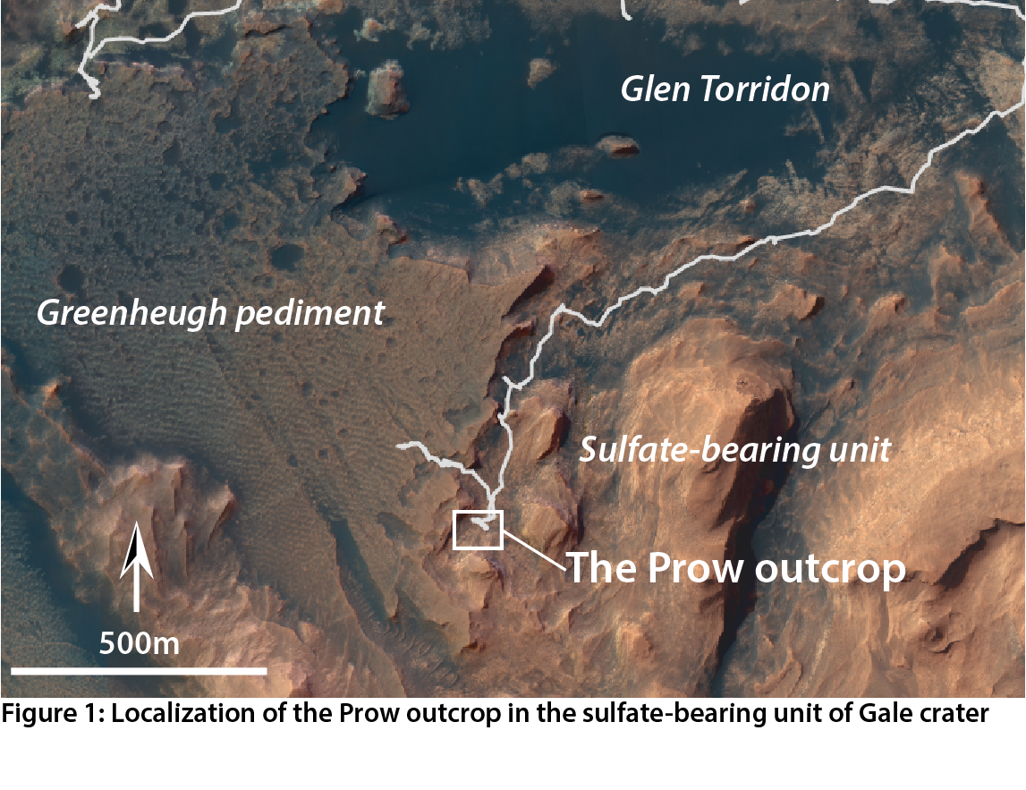
Such structures are notably well visible at the Prow locality, a major outcrop situated in the Contigo member of the Mirador formation, just below the Greenheugh pediment (Fig. 1). This outcrop has been reached and studied in January and February 2022, between sols 3349 and 3379. Using ~3200 mid- and close-range images from the Navigation and Mast cameras (Navcam, Mastcam), we used structure-from-motion photogrammetry to reconstruct a Digital Outcrop Model (following the method described in [7]) of the Prow locality and its vicinity (Fig. 2). This DOM covers an area of about 1000m². Two small excerpts of this DOM are explorable online on the Sketchfab platform at https://skfb.ly/o8DJZ and https://skfb.ly/otpLW. The DOM allows us to visualize and characterize several sets of meter- to centimeter-scale sedimentary structures, over about 30 meters of lateral continuity, either using on-screen visualization, or integrated within a Virtual Reality environment.
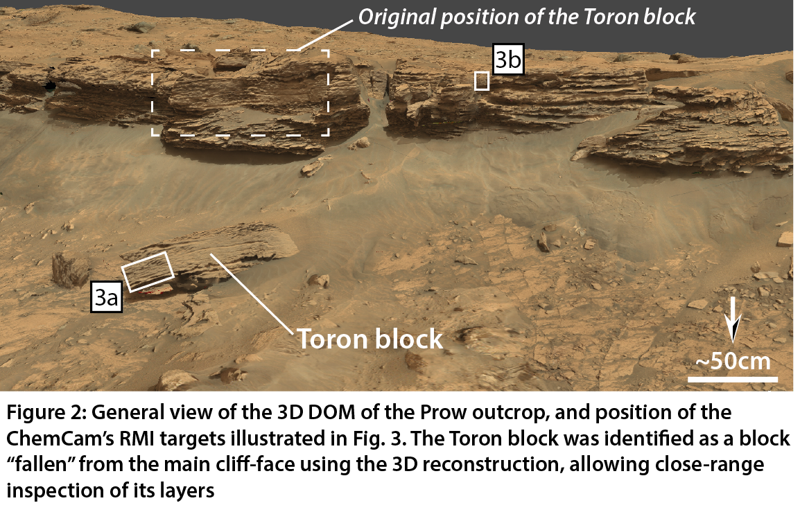
The DOM reconstruction has been helpful in determining the targets of interest during the Prow exploration by Curiosity. One particular benefit has been to identify the Toron block (Fig. 2) as a fallen piece of the main outcrop, allowing us to perform very close-range observations of the outcrop’s cliff-face (e.g., Fig. 3a) without actually putting the rover too close to the actual rock-face. The interest of using such 3D reconstruction notably lies in the ability to characterize the spatial distribution of the multi-scale structures observed at the Prow, but also to study the spatial distribution (and potential variations) of the geochemical composition of these layered sandstones as seen by the ChemCam instrument. We also take advantage of the high-resolution micro-images provided by the Remote Micro-Imager subsystem of the ChemCam instrument (with a field of view of 20 mrad per frame, resolving grains under the silt at close range) to study the facies (grain-size, micro-structures) of the different sandstone beds cropping out at this locality (Fig. 3).
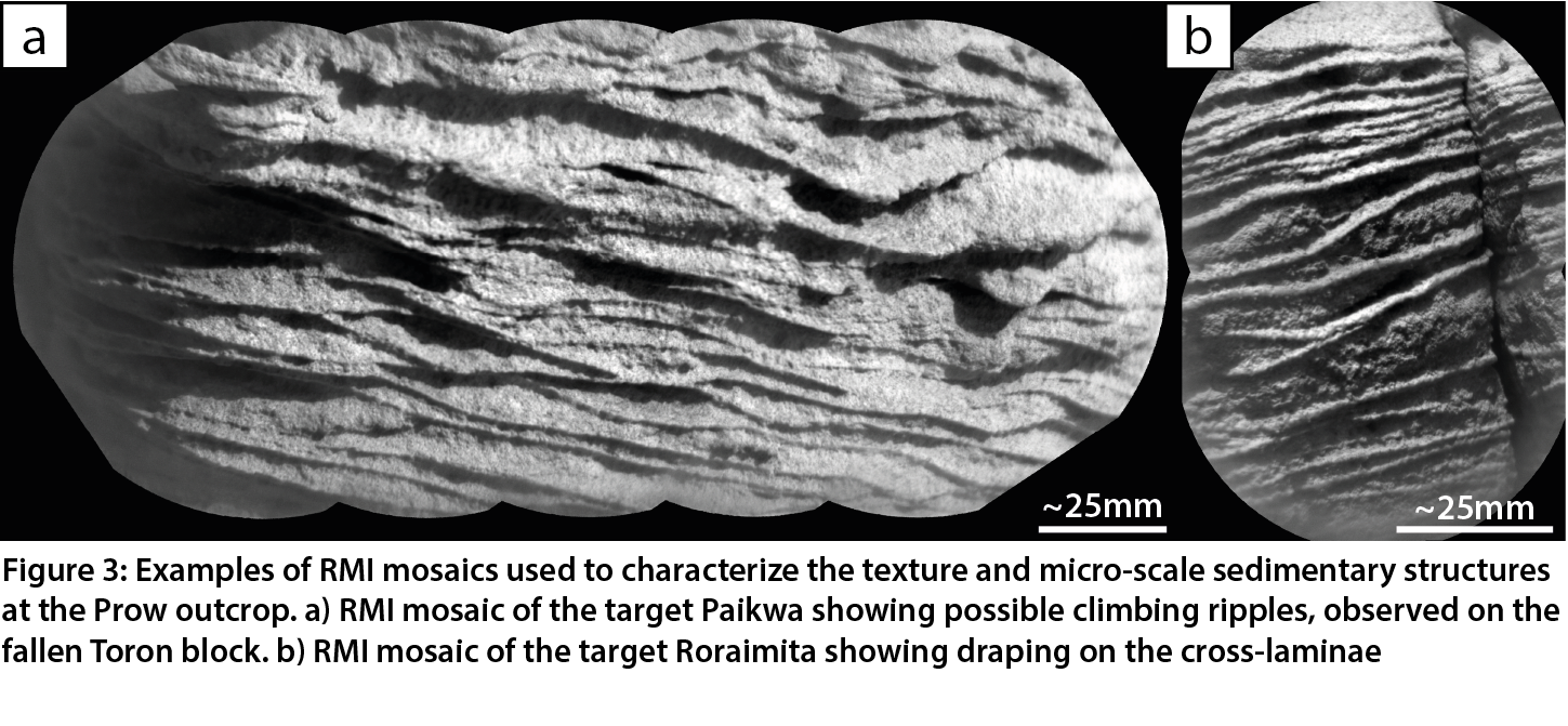
At the Prow, we characterize several sets of sedimentary structures such as (but not limited to) meter-scale cross-stratifications, cm-scale symmetric ripples but also probable climbing ripples (Fig. 3a). These structures, mostly indicating a direction of transport toward the NW (similar to what is observed in underlying Glen Torridon area), denotates sustained aqueous conditions compatible with a fluvial setting. We also observe in some place at the Prow, and notably in the upper layers, mm-scale fine-grained draping (Fig. 3b) deposited at the surface of (cross-)stratifications, reminiscent of flaser bedding on Earth. These fine muddy levels indicate recurrent intervals of low-energy deposition in-between higher-energy periods. Put together, these elements help us to characterize sustained aqueous conditions in a dynamic setting of combined flow and wave action at the time the sediments were deposited (e.g., [8]), helping us to determine probable mixed fluvio-aeolian settings around the critical climatic transition observed within this sulfate-bearing unit characterized by alternating wet and dry conditions.
References: [1] Miliken et al., 2010, Geophys. Res. Lett. 37, L04201; [2] Rapin et al., 2021, Geology 49; [3] Caravaca et al., 2021, Remote Sensing, 13(20), 4068; [4] Rapin et al., 2022, EPSC, this meeting; [5] Schieber et al., 2022, LPSC, Abstract #1304; [6] Meslin et al., 2022, LPSC, Abstract #2492; [7] Caravaca et al., 2020, Planet. Space Science 182, 104808 ; [8] Gupta et al., 2022, ESPC, this meeting.
How to cite: Caravaca, G., Le Mouélic, S., Gupta, S., Mangold, N., Rapin, W., Schieber, J., Le Deit, L., Gasnault, O., and Lanza, N. L.: The Prow outcrop: an “open catalog” of multiscale 3D fluvial sedimentary structures in the lower sulfate unit of Gale crater (Mars), Europlanet Science Congress 2022, Granada, Spain, 18–23 Sep 2022, EPSC2022-336, https://doi.org/10.5194/epsc2022-336, 2022.
Introduction: Martian valley networks are evidence of ancient flowing water [1-3] during the Late Noachian to Early Hesperian period (3.7-3.5 Ga), likely as a result of precipitation-fed fluvial incision [4-5]. Mars is also home to paleolake outlet canyons, which formed as water accumulates within an impact crater's interior, forming a paleolake that eventually overflows, breaching the crater rim and causing flooding and incision of the outlet canyon over weeks to years [6-7]. The flow velocity is substantial enough to overcome topography. It has been hypothesized that valley networks that form after the outlet canyons may follow the troughs carved by them [6].
Valley formation rapidly decreased after the Early Hesperian (~ 3.7 Ga) indicating a waning water cycle. Evidence for the loss of water may be observed in valleys and paleolake outlet canyons. For example, Williams et al. (2001) [8] measured the width and depths of thousands of valleys, finding that some become narrower and shallower down their profiles, indicative of water loss down the valley.
In this study, we examine two paleolake outlet canyons with decreasing widths down-profile, which are adjacent to the Tharsis Rise, by applying paleohydraulic, morphometric, and morphological calculations. Examining these canyons will reveal information about their influence on adjacent valley networks. Additionally, the proximity of these canyons to faults associated with Tharsis deformation may reveal insight into the chronology between the formation of Tharsis and fluvial activity. Studies are currently divided on which formed first [9-12]. Furthermore, we aim to determine if valley systems display any evidence of water loss.
Data and Methods: Mapping was performed in QGIS, using MRO Context Camera (CTX) images (5 m/pixel) [18] and the Viking Digital Image Model (MDIM) [19] map (231 m/pixel) for the missing regions. Length, width, and slope (elevation taken from individual MOLA shots) values were extracted from the mapped valleys and outlet canyons. Discharge values were calculated down the paleolake outlet canyon's profile for both valleys and interior channels [13-14]. The MOLA Digital Elevation Model (DEM) (463 m/pixel) [20] was used to perform palaeohydraulic equations [15]. Hack's law (L = C*Ah; where, L is valley length, A is drainage area, and C and h are constants) was applied to valley networks running into the paleolake outlet canyon [15]. A h value between 0.5 and 0.6 is expected for precipitation-fed valley networks [15, 16]. In addition, we provide a valley depth cross-section down profile to probe if there is evidence of water loss.
Results: Our mapping revealed that these valley systems have experienced a diverse history of fluvial activity. The second valley system displays the remains of ancient hanging valleys (Figure 1) that are dissected by faults. The paleolake outlet canyon cuts through these faults. Finally, adjacent valley networks, one of which is at the source of a central channel within the outlet canyon, incise the valley walls of the paleolake outlet canyon. Knickpoints are observed within the elevation profile of one of the adjacent valley networks (Figure 2). From the discharge relationships for both valleys and interior channels, we have found a difference in discharge values on the order of magnitude ~103 m3/s.
Two of the adjacent valleys have a h value within the expected range for precipitation-fed networks, and the rest do not. Additionally, we observe disturbances in the valley's elevation profiles adjacent to the paleolake outlet canyon.
Although valley networks join the main outlet canyon, we measure no increase in width or depth after the introduction but measure a general decrease in width and depth (i.e., overall cross-sectional area) down the outlet canyon profile.
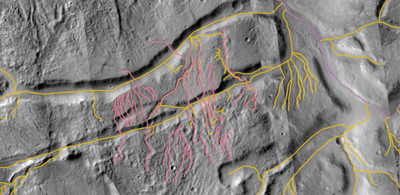
Figure 1. A section of the second valley system. Displayed are the hanging valleys (pink), remains of older valleys, and the faults (yellow) that are disrupted by the paleolake outlet canyon (purple) overlaid on CTX images.
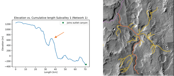
Figure 2. Left: Elevation profile of adjacent valley with a knickpoint (see orange arrow). Right: Associated valley (orange) with tributaries (yellow) connected to a paleolake outlet canyon (purple).
Discussion: These valley systems appear to have experienced the following chronology: (1) Ancient fluvial activity, resulting in remnant hanging valleys. (2) Tectonic activity, potentially associated with Tharsis, resulting in the production of faults that cross-cut the hanging valleys. (3) Paleolake outlet canyon incision, indicating substantial fluvial activity during this period. (4) Valley network formation, resulting in the incision of the walls of the outlet canyon. Knickpoints within these valleys [17], and the presence of channels possibly associated with these valleys within the outlet canyon, indicate that these valleys were potentially active after the paleolake outlet canyon ceased to be active. These channels, and the lack of conformity between the valleys and topographic adjacent to the outlet canyons, indicate that the valleys have followed the predefined trough formed by the canyons. These systems indicates that valley formation occurred before, potentially during, and after deformation associated with the formation of the Tharsis Rise.
The decrease in width, depth, and discharge of the paleolake outlet canyons down their profile indicates that there has been a loss of water. The cause of this water loss is currently unclear, however, it may aid in understanding the reduction of Mars’ water cycle.
References: [1] Masursky, H. (1973) JGR, 78(20). [2] Hynek, B et al., (2010) JGR: Planets, 115(E9). [3] Pieri, D. C. (1980) Science, 210(4472). [4] Jaumann, R. et al. (2005) Geophysical Research Letters, 32(16). [5] Carr, M. H., & Malin, M. C. (2000) Icarus, 146(2). [6] Goudge, T. A. et al., (2021) Nature, 597(7878). [7] Fassett, C. I., & Head III, J. W. (2008) Icarus, 198(1). [8] Williams, R. M., & Phillips, R. J. (2001) JGR: Planets, 106(E10). [9] Phillips, R. J. et al. (2001) Science, 291(5513). [10] Bouley, S. et al., (2016) Nature, 531(7594). [11] Black, B. et al., (2017) Science, 356(6339). [12] Bahia, R. S. et al., (2022) Icarus, 115041. [13] Irwin III, R. P. et al., (2005) JGR: Planets, 110(E12). [14] Gou, S. et al., (2019) Icarus, 328. [15] Hack, J. T. (1957) (Vol. 294). US Government Printing Office. [16] Bahia, R. S., et al., (2019) 50th LPSC, 1197. [17] Duran, S. et al., (2019) Scientific reports, 9(1). [18] Malin et al., (2007), JGR: Planets, 112. [19] http://astrogeology.usgs.gov/maps/mdim-2-1 [20] Smith, D. E. et al. (2001). JGR, 106(E10).
How to cite: Diamant, S., Bahia, R., Miguel, Y., and Sefton-Nash, E.: Martian Paleolake Outlet Canyons - Evidence for Controls on Valley Network Formation and a Waning Water Cycle, Europlanet Science Congress 2022, Granada, Spain, 18–23 Sep 2022, EPSC2022-268, https://doi.org/10.5194/epsc2022-268, 2022.
Fluvial landforms on Mars are important because they indicate past liquid water. The landforms can provide information about past environmental and climate conditions and the potential for past life. Ancient fluvial sediment transport fluxes have been estimated for several channels on Mars. However, it is also important to understand the differences between sediment transport on Earth and Mars. Fluxes can differ significantly due to gravity, sediment density, lack of ecology and the possible presence of ice. Only when we understand the effects of such differences on sediment fluxes, we can apply and adapt knowledge of fluvial geomorphology on Earth to the surface of Mars. Additionally, such understanding will greatly improve the use of Earth analogues.
In this study, we isolate the effects of gravity on fluvial sediment transport with a 1D model of a simple static channel and a 2D depth-averaged numerical hydro-geomorphological model of a growing delta. The results show that sediment transport on Mars is more efficient than on Earth for the same water discharge, sediment distribution, and channel geometry. The 1D results show that mainly fine sediment is transported more efficiently on Mars, because the effect of gravity is stronger on suspended transport compared to bedload transport and bigger grains travel in suspension on Mars compared to Earth for the same boundary conditions. Because gravity affects fine and coarse sediment fractions differently, we also expect differences in geomorphology due to different ratios of sediment fractions and disparities in sediment sorting. We are exploring these morphological effects in our 2D delta model. Our preliminary results suggest that the lower gravity on Mars results in faster-growing deltas with lower slopes and wider channels. These results suggest that unexpected differences with Earth might also occur in the delta stratigraphy, which is important to realise when drilling for sediment samples in the search for biosignatures.
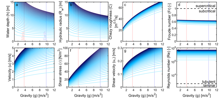
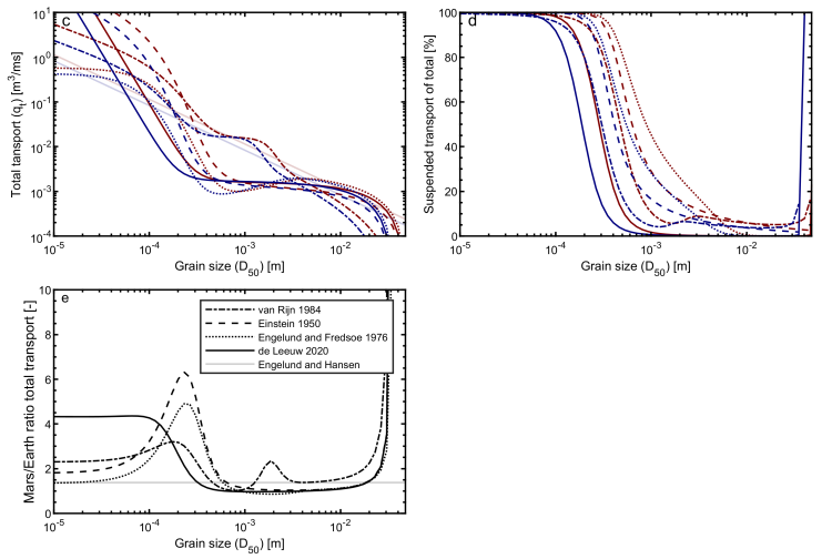
How to cite: Braat, L. and Lamb, M. P.: Isolated effects of gravity on sediment fluxes and delta morphology, Europlanet Science Congress 2022, Granada, Spain, 18–23 Sep 2022, EPSC2022-356, https://doi.org/10.5194/epsc2022-356, 2022.
- Introduction
Jarosite (KFe3(SO4)2(OH)6) was found by rover Opportunity in Martian surface at Meridiani Planum as well as by Spirit at Gusev crater. This mineral needs specific conditions to be formed, such as acid pH and oxidant environment1. In addition, this mineral has been found in meteorites, related to other compounds like olivine, goethite or gypsum.
There are different hypothesis for the formation of jarosite from olivine. Hereunder, two of them are exposed.
The first one described the jarosite formation in nakhlite meteorites, when the olivine transform to iddingsite. Iddingsite is a mixture formed by smectite clays, iron oxides and ferrihydrite2. Besides, some studies propose that jarosite forms part of iddingsite3.
The formation of jarosite from olivine in iddingsite phase can be explained by the dissolution of the latter. The minerals formed depend on pH and the ions present in the solution. The formation of jarosite can be explained by these reactions, considering an olivine with 1.8 proportion of Mg and 0.2 of Fe4 which is dissolved in acid conditions (reaction 1).

To form jarosite, the cation Fe2+ must be oxidized to Fe3+ (reaction 2). Finally, this Fe3+ can react with dissolved sulphate to form jarosite. Depending on the presence of other cations in the solution, different types of jarosite can be formed.
Other hypothesis5 proposed for the formation of jarosite can be made considering that in the history of Mars there were cold and dry climate periods. Moreover, in Mars there was also a high volcanic activity that formed sulphate-rich deposits. Considering this, Niles et al.5 suggested that olivine grains in Martian surface could form Fe-rich sulphates, as jarosite, if they were exposed to H2SO4 rich aerosols at temperatures around -40 °C (cryogenic conditions). The cations needed to form jarosite could be incorporated from different minerals, being olivine the most important source5.
In Martian nakhlite Miller Range 090030 (MIL 090030), jarosite has been found next to olivine and rasvumite (KFe2S3) recurrently. This fact, lead to the assumption that they were related. However, to this day, no explanation for the presence of jarosite together with rasvumite and olivine has been proposed. In this study, a hypothesis for an alternative formation of jarosite is made based on Raman image analyses carried out on the MIL 090030 Martian meteorite.
- Materials and method
A thick slide of the MIL 090030 meteorite was analyzed by means of Raman spectroscopy image. For this aim, an inVia confocal micro-Raman spectrometer, provided with 785 nm and 532 nm excitation lasers and CCD detector, was used coupled to HR StreamLine Imager.
- Results and discussion
After detecting all minerals around olivine grains in the bulk of the meteorite, the distribution of the different mineral phases can be obtained using Raman image. In this way, Figure 1 shows the mineral distribution of a rasvumite/jarosite rich region in MIL 090030. Moreover, it can be appreciated how jarosite and rasvumite are surrounded by magnetite and cristobalite.
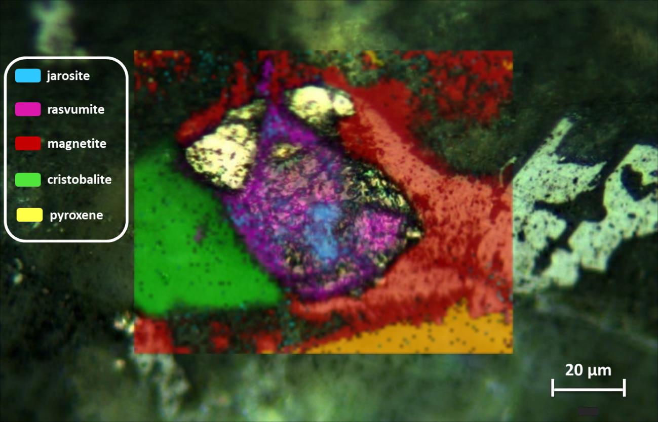
Figure 1. Raman image performed on the MIL090030 meteorite in a rasvumite/jarosite rich region.
Based on the findings detected in the analysed MIL 090030 fragment, the formation of jarosite from olivine and rasvumite is proposed following these four reactions:

On the one hand, rasvumite could react with H2O and O2 from Martian atmosphere to form magnetite (Fe3O4) (reaction 4). The soluble ions formed can arrive to other zones of the Martian surface travelling through cracks and pores.
The protons formed in reaction 4 can dissolve partially the olivine giving rise to an olivine richer in forsterite (reaction 5). The SiO2 formed can be dissolved in water to form H2SiO3 or H4SiO4. This solution can then precipitate as quartz when water evaporates.
On the other hand, rasvumite can react also directly with H2O and O2 to form jarosite and free sulphate anion (reaction 6). Sulphate anions formed in reactions 4 and 6, can interact with iron cations from reaction 5 and potassium cations from reaction 4 to form jarosite (reaction 7).
The high pressures and temperatures reached during the impacts suffered by the meteorite can alter some minerals present in the meteorite. In the MIL 090030 meteorite, quartz was not detected. Instead of this mineral phase, its high temperature and pressure polymorphs (cristobalite, coesite and stishovite) were detected in the rasvumite/jarosite rich region. The presence of these polymorphs indicates that the reactions 1-4 occurred in Mars.
- Conclusions
According to the mineral distribution in MIL 090030, based on Raman image results, an explanation for the formation of jarosite from olivine and rasvumite is proposed. This formation is related to reactions of rasvumite with Martian atmosphere compounds and dissolution of olivine from the Martian surface.
- Acknowledgments:
Authors are grateful to NASA for accessing to the MIL 090030 Martian meteorite sample through the loan agreement between NASA's JSC and the UPV/EHU. This work has been funded by the “Raman On Mars” project (Grant No. PID2019-107442RB-C31), funded by the Spanish Agency for Research (MICINN and the European Regional Development Fund), and the “Study of Alteration Processes in Terrestrial and Planetary materials” strategic project (ref. PES 21/88), funded by the University of the Basque Country (UPV/EHU.
- Bibliography:
1) Papike, J.J., Karner, J.M., Shearer, C.K.: Comparative planetary mineralogy: implications of martian and terrestrial jarosite. A crystal chemical perspective, Geochim. Cosmochim. Acta., Vol. 70, pp. 1309-1321, 2006.
2) Swindle, T.D., Treiman, A.H., Lindstrom, D.J., Burkland, M.K., Cohen, B.A., Grier, J.A., Li, A., Olson, E.K.: Noble gases in iddingsite from the Lafayette meteorite: evidence for liquid water on Mars in the last few hundred million years. Meteorit. Planet. Sci., Vol. 35, pp. 107-115, 2000.
3) Noguchi, T., Nakamura, T., Mizawa, K., Imae, N., Aoki, T.,Toh, S.: Laihunite and jarosite in the Yamato 00 nakhlites: Alteration products on Mars? J. Geophys. Res., Vol. 114, 2009.
4) King, H.E., Plümper, O.,Geisler, T.,Putnis, A.: Experimental investigations into the silicification of olivine: Implications for the reaction mechanism and acid neutralization. Am. Min., Vol. 96, pp. 1503-1511, 2011.
5) Niles, P.B., Michalski, J., Ming, D.W., and Golden, D.C. Elevated olivine weathering rates and sulphate formation at cryogenic temperatures on Mars. Nat. Commun., Vol. 8, 2017.
How to cite: Madariaga, J. M., Coloma, L., Aramendia, J., Huidobro, J., Poblacion, I., Garcia-Florentino, C., Castro, K., and Arana, G.: Jarosite formation from olivine and rasvumite in Martian meteorite MIL 090030, Europlanet Science Congress 2022, Granada, Spain, 18–23 Sep 2022, EPSC2022-518, https://doi.org/10.5194/epsc2022-518, 2022.
The geologic origin of the ancient, phyllosilicate-rich bedrock at Oxia Planum, Mars, the landing site of ESA’s ExoMars rover, is unknown. The phyllosilicates record ancient aqueous processes, but the processes that formed the host bedrock remain elusive. Here, we use high-resolution orbital image and topographic datasets (HiRISE, CTX, CaSSIS) to investigate and characterize fluvial sinuous ridges (FSRs), found across the Oxia Planum region. The FSRs form segments up to 70 km long, with sub-horizontal layering commonly exposed in ridge margins. Some FSRs comprise multi-story ridge systems; many are embedded within and are being exhumed from the phyllosilicate-rich bedrock. We interpret the FSRs as deposits of ancient, episodically active, alluvial river systems (channel-belt and overbank deposits) at Oxia Planum. Thus, the phyllosilicate-rich bedrock was formed at least partly by ancient alluvial rivers, active across the wider region. Our alluvial hypothesis does not exclude other sources of sediment playing a role in building the terrain as well. Future exploration by ExoMars can verify this interpretation and provides an opportunity to investigate some of the oldest river deposits in the Solar System.
How to cite: Davis, J., Balme, M., Fawdon, P., Grindrod, P., Favaro, E., and Banham, S.: Ancient Alluvial Plains at Oxia Planum, Mars, Europlanet Science Congress 2022, Granada, Spain, 18–23 Sep 2022, EPSC2022-545, https://doi.org/10.5194/epsc2022-545, 2022.
Introduction.
Earth's most-ancient crust has been recycled through plate tectonics processes making it unlikely that we will ever directly sample it (although, one can imagine finding ancient Earth meteorites one the Moon [1].) Mars, on the other hand, hosts ancient crustal outcrops on its surface. The uplifted massifs surrounding Argyre, Hellas, and Isidis – the three largest, well-preserved impact basins on Mars - formed in the chaotic aftermath of the basin-forming impacts due to normal faulting caused by crustal thinning from impact excavation [2]. Our goal is to understand the igneous minerals associated with uplifted massifs using the Compact Reconnaissance Imagining Spectrometer for Mars (CRISM) [3] around Argyre, Hellas, and Isidis (Fig. 1). Here, we present initial results in this effort for the north Hellas area and expect to present preliminary results for Argyre and Isidis, as well, at the conference.
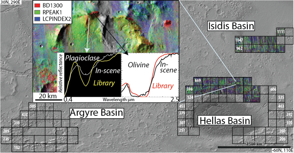
Fig. 1 Context view of the study area. Squares outline 5°x5° CRISM tiles. Number of tiles is 100, covering an approximate 5% of the surface. CRISM coverage is >80 % over tiled areas. Inset shows a region at the map scale of 1:250,000 with CRISM spectra of uplifted massifs compared to library spectra. In the spectral parameter combination, red is consistent with olivine, yellow with plagioclase, and blue with low-calcium pyroxene.
Methods.
CRISM Data Processing. We used CRISM multispectral mapping data (MSP) and hyperspectral mapping data (HSP). The MSP mapping strips have 19 visible to near-infrared (VNIR, 0.4-1 µm) spectral channels and 55 short-wavelength infrared (SWIR, 1-4 µm) channels, and the HSP mapping strips contain 107 VNIR channels and 154 SWIR channels. Both mapping datasets have a ground sampling distance of approximately 180 m. The set of wavelength channels contained in the MSP dataset were chosen to sample more densely in wavelengths regions known to contain absorption features of minerals likely to be detected on Mars (primary rock-forming silicates, phyllosilicates, etc. [3]). For our study, HSP data were resampled to the MSP wavetable to increase the spatial coverage. Typical coverage of the MSP+HSP dataset is ~85%, with sufficient overlap to allow for mosaicking and radiometric reconciliation. We processed these data through a custom pipeline [4] that includes initial noise filtering, photometric and atmospheric corrections [5], [6], and an empirical correction for “spectral smile” [7]. The final products of this pipeline are 5°x5° mosaic tiles with improved inter-strip variability in atmospheric residuals [8].
A typical method for condensing the information contained in a CRISM image into an interpretable form is by calculating “spectral parameters”, i.e., mathematical summations of particular characteristics of the spectra [9]. Spectral parameters can be combined into 3-band RGB images that highlight specific, thematically-related, combinations of interest. Fore example, the MAF summary product combines indexes intended to highlight mafic mineralogy: olivine (OLINDEX3), low-calcium pyroxene (LCPINDEX2), and high-calcium pyroxene (HCPINDEX2). From the CRISM mapping tiles, we constructed summary products that are well-suited for compositional mapping over large areas [10] (e.g., Fig. 1).
Compositional Mapping. Regions of interest were identified with the map tile summary products in ArcGIS followed up by detailed spectral analyses in IDL/ENVI (specialized software for analyzing hyperspectral images) with custom add-on analysis tools. Point locations of compositions, confirmed through spectral analysis, were imported back into ArcGIS and “outcrops” were mapped using summary products. We define outcrop in the context of this work as a spatially contiguous region with an internally consistent spectral signature distinct from its surroundings (e.g., Fig. 2).
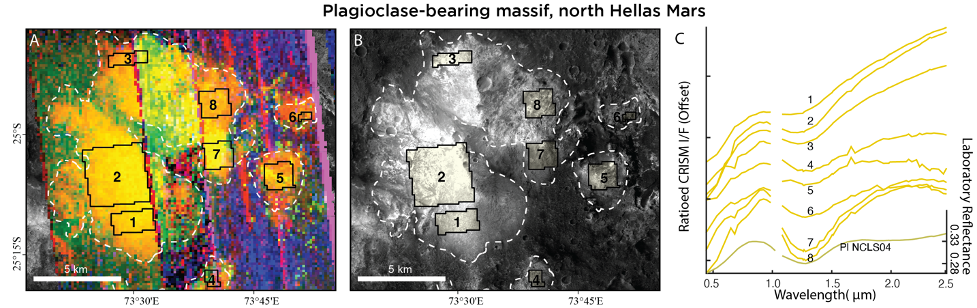
Fig. 2 Example plagioclase-bearing massif north of Hellas basin. (A) CRISM browse product (same as in Fig. 1). Yellow tones are consistent with plagioclase. Black boxes indicate 8 regions over which spectra were taken and plotted in C. (B) CTX 5 m/pixel image of the same massif as in (A). White dashed lines denote outcrops mapped in this A and B. (C) Average CRISM ratioed I/F spectra from the 8 regions indicated in A and B.
Results and Discussion.
Thus far, we have mapped 12 high-calcium pyroxene-bearing outcrops, 97 plagioclase-bearing outcrops, 128 LCP-bearing outcrops, and 129 olivine-bearing outcrops (Fig. 3). Outcrops with distinct mineralogical signatures are often observed adjacent to each other on the same massif, or on massifs in close spatial proximity (relative to the size of the massifs, ~several kilometers). We also identified Fe-, Mg-, and Al-phyllosilicate minerals associated with the massifs and, more commonly, with impact crater ejecta along the northern Hellas rim.
The number and spatial extent of plagioclase-bearing outcrops was surprising and is described in [11]. The massifs pre-date Hellas (≥ 4.1 Ga) and are situated stratigraphically above putative mantle material. The north Hellas massif outcrops may expose the remains of an ancient large igneous complex, perhaps similar to terrestrial layered mafic intrusions. Preliminary results from the Argyre and Isidis uplifted massifs will be presented at the conference and compared to those from north Hellas.
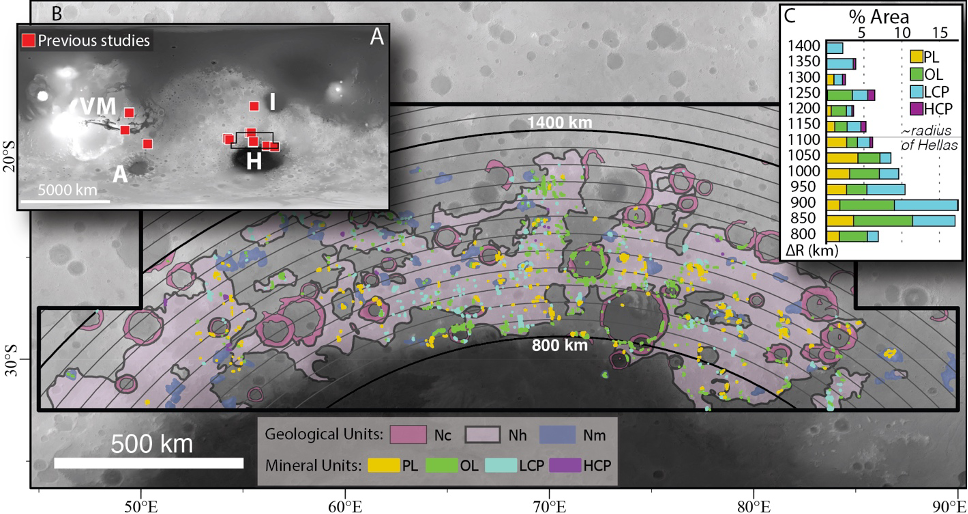
Fig. 3 Summary of detections over north Hellas. (A) Red squares indicate all locations of plagioclase-rich outcrops discovered previous to our work. (B) Context map showing all mafic mineral outcrops mapped in our study. Arcs are 50-km interval bins measured radially from the center of Hellas. Geologic units are Noachian crater (Nc), Noachian highland (Nh) and Noachian massif (Nm) from Leonard and Tanaka, 2001. (C) %Area is the area of each mineral outcrop normalized to the area of the Nc, Nh, and Nm geologic units in each radial bin. Note the concentration of detections interior to the nominal radius of Hellas, highlighting the stratigraphically low position of the outcrops.
[1] J. J. Bellucci et al. doi: 10.1016/j.epsl.2019.01.010.
[3] G. J. Leonard and K. L. Tanaka, 2001.
[4] S. L. Murchie et al. doi: 10.1029/2009je003344.
[5] F. P. Seelos and S. L. Murchie, LPSC. p. 2325, 2018.
[6] F. P. Seelos, et al., LPSC. p. 1783, 2016.
[7] F. Morgan et al., LPSC. p. 2453, 2011.
[8] F. P. Seelos et al., LPSC. p. 1438, 2011.
[9] F. P. Seelos, et al., LPSC p. 2635, 2019.
[10] C. E. Viviano‐Beck et al. doi: 10.1002/2014JE004627.
[11] C. E. Viviano et al., LPSC, p. 1485, 2020.
[12] Phillips, M. S., et al., Geology, accepted.
How to cite: Phillips, M., Viviano, C., Moersch, J., Rogers, A. D., and Seelos, F.: Mars uplifted massifs: unique and extensive samples of ancient crust., Europlanet Science Congress 2022, Granada, Spain, 18–23 Sep 2022, EPSC2022-736, https://doi.org/10.5194/epsc2022-736, 2022.
Abstract
Northwestern part of Terra Cimmeria displays a wide range of fluvial, lacustrine and glaciofluvial geomorphological features, indicative of presence of liquid water in this area early in the Martian history. These features were previously mapped as part of global studies, but not in relation to the area itself. Here we present our reconstruction of hydrologically correct model of northwestern Terra Cimmeria based on algorithm assisted mapping exercise of unprecedented precision. Based on our findings we are able to contextualize the geomorphological specifics of individual subbasins within the framework of Late Noachian Icy Highlands model and subsequent climatic transition towards the dry and cold state of the Amazonian period.
Physiographic Characteristic
Terra Cimmeria is an extensive region of the Martian southern highlands. Its northwestern portion (Northwestern Terra Cimmeria, NWTC) lies in the equatorial area of the planet and likely did so even before the Tharsis-induced true polar wander event (Bouley et al., 2016). It is nested between the volcanic province of Hesperia Planum to the southwest and the Utopia highland-lowland boundary to the north (Skinner and Tanaka, 2007). In the setting of the disputed Arabia Level ocean shoreline (Sholes et. al, 2021 and references therein) NWTC would stand out as the longest peninsula on Mars. The surface of NWTC is dominated by the Late Noachian highland unit with „undifferentiated impact, volcanic, fluvial and basin material“ (Tanaka et al., 2014). There are several open-basin lakes as mapped by Fassett and Head (2008), craters in different stages of degradation, and numerous valley networks which dissect the terrain (Carr, 1995; Hynek et al., 2010; Alemanno et al., 2018) and few on which terminate as deltaic deposits previously mapped by Achille and Hynek (2010). The variety and density of geomorphological features whose formation is tied to the presence of volatiles suggests a rich history of fluvial, lacustrine, and glaciofluvial activity and importantly fluvially dominated erosion and deposition. We incorporated available imagery and previously derived datasets in our algorithm assisted mapping exercise in order to contextualize the putative sources of the valley carving runoff within the local climatic background.
Methodology
NWTC valley networks were mapped several times in different level of detail starting with Carr (1995) who based his mapping on Viking imagery. This initial campaign was followed by Hynek et al. (2010) who utilized THEMIS daytime IR imagery and MOLA DEM and later by Alemanno et al. (2018) who in addition to THEMIS daytime IR and MOLA DEM used the ConTeXt (CTX) camera imagery to improve their recognition capability where the forementioned datasets lacked sufficient resolution.
Our mapping is based on the high resolution global CTX image mosaic rendered at 5 m/pixel (Dickson et al., 2018), THEMIS nighttime IR dataset, and MOLA DEM with the vectorized valley network dataset of Alemanno et al. (2018) serving as a baseline. We used Whitebox GAT surface flow accumulation model with hybrid breaching-filling sink removal capability (Lindsay, 2015) to digitalize the thalwegs as well as subbasins based on MOLA DEM. The algorithm-derived thalwegs and previously mapped valley networks were used to guide and double check the manual mapping which was based strictly on the CTX and THEMIS nighttime IR mosaics. Subsequently, digitalized subbasin borders were checked against the CTX mosaic and corrected based on the underlaying terrain. Notable geomorphological features were identified and marked as point features and putative headwater areas we delineated based on the previously logged data.
Results
We mapped an area spanning more than 8✕105 km2 and reconstructed 7 main valley networks. The valley networks were divided into over 80 subbasins based on manual correction of flow accumulation model. We managed to identify and connect seemingly isolated stretches of valleys and incorporate them into their respective networks thus creating a hydrologically correct reconstruction of the area. We identified several headwater-specific geomorphic features, pingos and paleolakes.
Discussion
In Noachian NWTC was situated between the equilibrium and terminus lines of a Late Noachian Icy Highlands (LNIH) ice sheet (Fastook and Head, 2015) and as such it would favor the formation of subglacial channels fed by meltwater (Galofre et al., 2020) and accumulation of ice (Wordsworth et al., 2013; Fastook and Head, 2015). The presence of developed dentritic networks which could have been carved by glavial meltwater is proven by our mapping exercise. Head et al. (2022) proposed that the climate of Mars underwent a transitional period during which a decrease in the atmospheric pressure induced a shift from altitude dependent temperature regime typical for the Noachian period (Wordsworth et al., 2013) towards latitude dependent temperature regime of the Amazonian period. This transition would start with ablation and melting of the lower altitude icy deposits and end with desiccation of equatorial ice reservoirs – both of which are in broader sense applicable to NWTC. In the beginning of this transitional period, meltwater released during the phases of peak temperatures would return to the highland cold traps in the time between these episodes. It is therefore plausible that given the specific combination of altitude, latitude, and location of NWTC, this area could sustain active surface or near-subsurface hydrology for an extended period of time up to 106 -108 years. This is supported by the variety of geomorphic features present in NWTC, but remains to be further tested with buffered crater counting and development of conceptual and hydrological models based on the newly created datasets.
Acknowledgements
VC & YM were supported by Czech Science Foundation (#20-27624Y).
References
Carr, Michael H. (1995), doi:10.1029/95je00260; Skinner, J. A., & Tanaka, K. L. (2007), doi:10.1016/j.icarus.2006.08.013; Fassett, C. I., & Head, J. W. (2008), doi:10.1016/j.icarus.2008.06.016; Achille, G. D., & Hynek, B. M. (2010), doi:10.1038/ngeo891; Hynek, B. et al. (2010), doi:10.1029/2009je003548; Wordsworth, R et al. (2013), doi:10.1016/j.icarus.2012.09.036; Tanaka, K. L. et al. (2014), doi:10.3133/sim3292; Fastook, J. L., & Head, J. W. (2015), doi:10.1016/j.pss.2014.11.028; Bouley, S. et al. (2016), doi:10.1038/nature17171; Lindsay, J. B. (2016), doi:10.1002/hyp.10648; Alemanno, G. et al. (2018), doi:10.1029/2018ea000362; Dickson, J. et al. (2018). A Global, Blended CTX Mosaic of Mars with Vectorized Seam Mapping: A New Mosaicking Pipeline Using Principles of Non-Destructive Image Editing; Galofre, A. G. et al. (2020), doi:10.1038/s41561-020-0618-x; Sholes, S. F. et al. (2021), doi:10.1029/2020je006486
How to cite: Cuřín, V. and Markonis, Y.: Reconstruction of Northwestern Terra Cimmeria Watersheds, Europlanet Science Congress 2022, Granada, Spain, 18–23 Sep 2022, EPSC2022-549, https://doi.org/10.5194/epsc2022-549, 2022.
The stratigraphy preserved within Aeolis Mons (Mount Sharp) in Gale crater (Mars) shows a major transition from mudstone-rich strata (with subordinate sandstones) recording deposition in lacustrine to fluvial settings into a major sulphate-bearing unit (the Layered Sulphate-bearing unit (LSu)) [1, 2]. This transition is interpreted to represent a major environmental change from wetter conditions toward a more arid palaeoclimate on early Mars. A stratigraphic section over this transition constructed along Curiosity’s traverse shows a vertical change from mudstones with interstratified sandstones of the Glasgow and Mercou members of the Carolyn Shoemaker formation into strata of the Pontours member which have a strong diagenetic overprint, and thence into large-scale cross-stratified sandstones of the Mirador formation that are interpreted to be the deposits of large, migrating aeolian dunes. The lower section of the LSu is dominated by stacked, cross-bedded facies with variable diagenetic overprint, that likely records a purely dry aeolian dune environment [3]. However, higher up in the studied section, approximately 80 m above the base of the Mirador formation, there is a transition into a succession still dominated by large-scale cross-beds but with interstratified lenses of a different sandstone facies. The presence of these lenses within large-scale cross bedded rocks is denoted by a transition to the Contigo member of the Mirador formation.
Whilst a number of lenses are visible in the stratigraphy of the Contigo member in cliffs along Curiosity’s traverse, the Mars Science Laboratory science team selected one lens, informally named The Prow to investigate in detail. Here, we describe the sedimentology of The Prow at a range of scales using Navcam, Mastcam, ChemCam Remote Micro-Imager(RMI), and Mars Hand Lens Imager (MAHLI) images with a focus on characterizing sedimentary structures, their depositional process interpretation and comparison to Earth analogs. The 3D geometries of The Prow’s sedimentary structures are analysed by [4].
The Prow was investigated during sols 3349 and 3379 in early 2022 and had been identified as a target of interest from long distance observations suggesting that it formed constrasting facies to surrounding rocks. The Prow is an ~18-m-long, ~0.5-1-m-thick lenticular sedimentary body that is interbedded with large-scale cross-stratified facies interpreted to be aeolian dune deposits. The nature of the lower contact of The Prow is unclear. The lens pinches out to the south.
The Prow shows a range of sedimentary structures suggestive of deposition under predominantly aqueous conditions. These structures differ from structures in surrounding bedrock indicating contrasting environmental conditions. The lowermost part of The Prow section appears to comprise decimetre-scale cross-beds indicative of deposition from subaqueous dune migration. The scale of these cross-beds is quite different from the large metres-scale trough cross-beds in rocks surrounding the lenses.
The upper sections of The Prow are dominated by cm-scale ripple structures well observed in cross-section. In particular, lenticular and flaser geometries are observed. Lenticular ripple forms with convex upper surfaces are common with concave lower surfaces where they overlie underlying ripple forms. The ripple forms occur vertically stacked and laterally offset. The individual lenses are commonly interconnected forming complex interwoven structures. The crests generally show rounded symmetric profiles. Locally, symmetric vertical accretion over ripple crests is observed implying rapid sediment aggradation. Many ripple forms do not appear to show internal lamination, although this may be due to a lack of grain size variation. In a few examples where internal lamination is observed, preserved foresets are suggestive of unidirectional flow.
RMI and MAHLI images reveal that ripple forms appear to have a finer-grained drape overlying ripple crests and extending into ripple troughs. MAHLI data confirm initial ChemCam observations and show that ripple cores comprise a sandstone and draping laminations are finer grained and likely below MAHLI-resolution (~60 microns). The drapes are provisionally interpreted as mud drapes formed from suspension fallout onto ripple topography during low energy quiescent episodes. The overall sedimentary geometry resembles flaser- to lenticular bedding common in Earth examples.
The symmetric form of many of the ripple structures with preservation of form sets is suggestive of formation by oscillatory flow by wave action. Locally, there is evidence of asymmetric accretion which is likely indicative of combined flow ripples. The presence of drapes of finer-grained material superimposed on coarser-grained ripple forms is interpreted to record episodes of higher-energy sand transport separated by recurrent intervals of low-energy conditions during which sand grains could not be mobilised. Wave and current activity caused bedload transport of sand constructing symmetric and asymmetric ripples. Between these episodes, there were quiescent periods where active flow ceased and finer-than-sand grains deposited out of suspension onto temporarily fossilised ripple forms. The preservation of stacked well-preserved ripple forms with crests intact suggests conditions of rapid deposition.
Locally, planar laminated beds with laterally continuous laminae are present; these maybe interpreted as either wind-ripple laminations formed by aeolian transport or as upper flow regime plane beds.
The presence of mudstone-draped wave and current ripple forms in the upper section of The Prow is strongly indicative of deposition from aqueous flows and moreover suggests the existence of a likely aerially small, shallow standing body of water in which the sediments were deposited. We compare the observed structures to forms observed in 1 Ga lake deposits from the Diabaig Formation of the Torridon Group (NW Scotland).
We tentatively infer that The Prow and by inference the other lenses observed in the Contigo member may record the episodic interdune or scour-fill presence of transient small standing bodies of water in an otherwise dominantly dry aeolian dune-dominated environment. The vertical transition from the underlying Dunnidear and Port Logan members of the Mirador formation that are dominated purely by large-scale trough cross bedding indicative of dry aeolian conditions indicates a change to a more mixed environmental setting with episodic fluvial/lacustrine activity perhaps from transient snow-melt or precipitation events occurring in otherwise arid conditions. Lenses such as The Prow demonstrate fluvio-lacustrine intervals punctuated dominant aeolian environment in the layered sulphate-bearing unit.
References: [1] Milliken et al., 2010, Geophys. Res. Lett. 37, L04201; [2] Rapin et al., 2021, Geology 49; [3] Rapin et al., 2022, EPSC, this meeting; [4] Caravaca et al., 2022, EPSC, this meeting.
How to cite: Gupta, S., Edgar, L., Yingst, R. A., Bryk, A., Caravaca, G., Dietrich, W., Grotzinger, J., Rubin, D., Rapin, W., Banham, S., Roberts, A., Le Mouélic, S., Williams, R., Schieber, J., Mangold, N., Kubacki, T., Gasnault, O., Wiens, R., Fraeman, A., and Vasavada, A.: Episodic aqueous conditions punctuated dominantly aeolian deposition within the layered sulphate-bearing unit, Gale crater (Mars), Europlanet Science Congress 2022, Granada, Spain, 18–23 Sep 2022, EPSC2022-963, https://doi.org/10.5194/epsc2022-963, 2022.
The overview
Evidence for water and aqueous processes during the initial infilling phase of Gale crater are abundant. Since 2012, the Mars Science Laboratory (MSL) rover Curiosity has investigated a variety of fluviolacustrine environments represented by the Bradbury and Mount Sharp groups. Both units accumulated as a result of sediment transport as bedload by fluvial processes, or by sediment settling from suspension in a lake. What is unclear is the duration that water persisted within Gale crater after the crater infilling was complete. In this contribution, we present evidence of water present within the base of the aeolian Stimson formation, which is recorded in the stratigraphic record by fluidization structures. We will describe the morphology of these structures, the mechanism of emplacement and implications for the history of aqueous processes in Gale crater.
The Background
The Stimson formation is the portion of a broader mound skirting unit which has been directly investigated by the MSL rover. This mound skirting unit unconformably drapes the northern flank of the present-day Mount Sharp. Where encountered on the traverse, the Stimson formation represents the preserved expression of an ancient aeolian dune field. Specifically, the stratigraphic record and the sedimentary architecture indicates that it was a dry dune field: water played no role in the accumulation of this sediment body. This fact is betrayed by the absence of fine-grained interdune deposits, microtopography, or other facies which are characteristic of water at or near the depositional surface. At the time the Stimson formation accumulated, Gale was devoid of surface water.
The Observations
Around Sol 3434, as Curiosity traverse onto the east side of the Greenheugh pediment, it encountered prominent erosion-resistant bedrock ridges which formed a polygonal (boxwork) network. These structures were observed in the basal portion of the Stimson formation, just a few metres above the base Stimson formation unconformity. Internally, these structures consisted of convolute, folded and warped laminations. Laterally, these structures were juxtapose against undeformed Stimson formation: large-scale cross-bedding composed of well-sorted medium-grained sandstones.
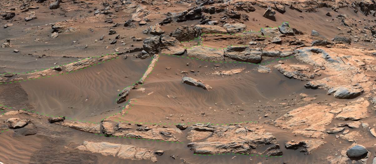
Figure1: Polygonal (boxwork) ridges observed at Feòrachas
Closer inspection of these internally-deformed ridge structures yielded evidence of both ductile displacement and destruction of primary stratification in a vertical orientation. The displacement and destruction are localised to the polygonal, linear ridges. Where stratification was displaced, laminations were folded into upright closed antiforms, with a tight bend radi on the hinge. Often, these are adjacent to open-folded synforms. Folding of laminations become tighter and more prominent with increasing vertical distance through the antiforms. Some original cross-laminations exhibited complex, recumbent folding where the underlying bounding surface exhibited open-folded synforms.
In some ridges, such as at the Lamington sandstone target, stratification was destroyed, and was replaced by continuous, vertically-oriented laminations that cross-cut horizontally-orientated laminations adjacent to the ridge (Figure 2). These laminations are oriented parallel to the long axis of the ridges, occasionally displaying vertical fold structures.
In some locations these erosion-resistant ridges contained vertically oriented fractures, with a few subordinate horizontal fractures, which were found to cross-cut some of the ductile deformation.
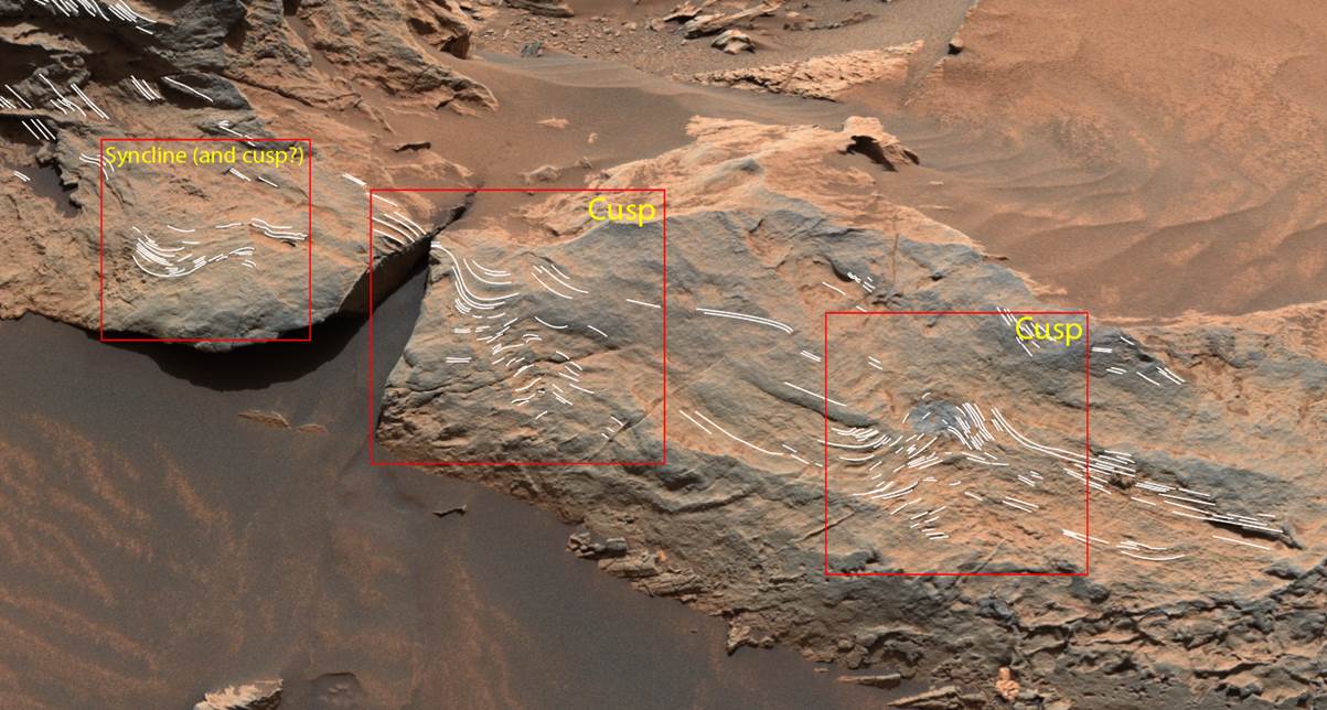
Figure 2: Close-up view of deformation structures within the Feorachas structure
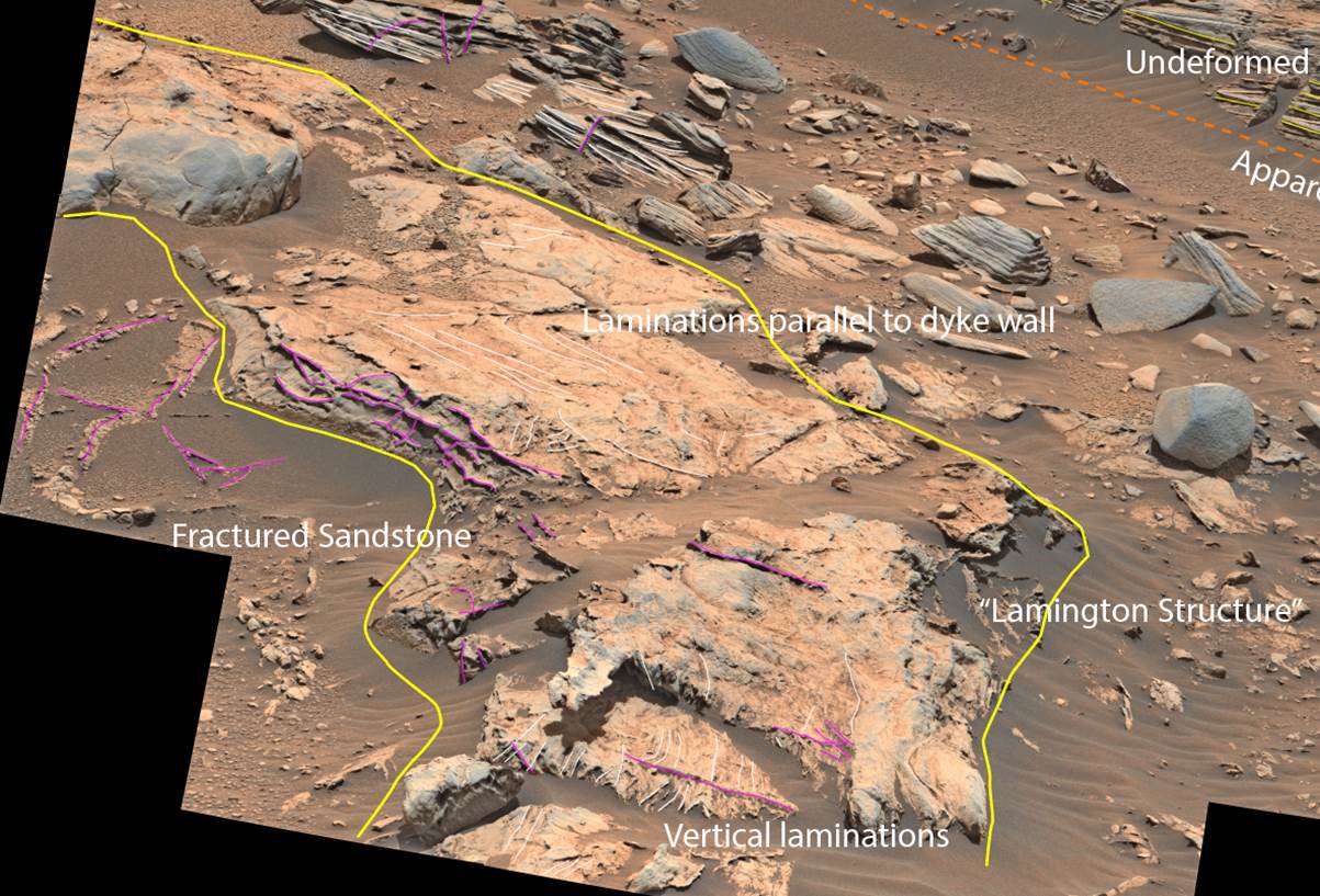
Figure 3: Lamington Sandstone: example of vertical laminations within a sand dyke
The Interpretation
These structures are interpreted to represent fluidization of sediment caused by water escaping through unconsolidated sediment, under pressure. The linear ridges such as the Lamington structure are interpreted to represent well-cemented sand dykes. The result is the partial or complete destruction of primary sedimentary structures (e.g. cross-bedding) and replacement with secondary sedimentary structures related with fluidization.
The tight antiforms are interpreted to be cusps while the vertical laminations are interpreted as pipes. Synforms, cusps and pipes exhibit pervasive vertical shear. The recumbent folding was also interpreted as evidence of vertical shear due to the displacement of the underlying bounding surfaces into vertical synforms. The vertical shear seen in cusp and synforms, and the vertical laminations observed in the dykes are evidence for the fluidization of sediment caused by upward fluid drag supporting the grain weight as water escapes through an open system under pressure. The source of the fluid may include groundwater upwelling or pore water from liquefaction occurring below the Stimson. As brittle deformation overprinted the soft sediment deformation, the trigger or cause of the fluidization may have been cyclic and caused brittle failure after the sediment regained its strength.
The implications
Regardless of the origin of the water, these fluidization structures provide evidence of persistent water within Gale crater after the exhumation of Mount Sharp, and the accumulation of the Stimson dune field. Presence of this water indicates:
- Water percolated into the base of the Stimson formation, either from fractures within the Mount Sharp group, from strata higher up on Mount Sharp, or from Meteoric sources.
- Water was present at the time which the Stimson formation was unconsolidated: which would be penecontemporaneous with dune field formation.
- This may represent a secondary habitable environment within the lithosphere.
How to cite: Banham, S., Roberts, A., Gupta, S., Dietrich, W., Bryk, A., Rubin, D., and Vasavada, A.: Fluidisation of Aeolian Sandstone in Gale crater: evidence for water post-dating exhumation of Mount Sharp, Europlanet Science Congress 2022, Granada, Spain, 18–23 Sep 2022, EPSC2022-748, https://doi.org/10.5194/epsc2022-748, 2022.
The Martian dichotomy features a 5.5 km contrasts in topography and a potential ~ 25 km difference in crustal thickness [1], depending on the crustal density assumption [2], between the older southern highlands and the younger northern lowlands. It is thought to be the most ancient feature observed on Mars and have formed within the first 400-500 Myr of Martian history [3].
While the formation mechanism of the dichotomy is still under debate, our previous models [4] have successfully demonstrated that a southern giant impact does not only form a thicker crust on the impacted site, but also have a significant consequence in the location of magmatism in the next billions of years. In addition to the shock wave-generated impact melt, the temperature within the mantle after a giant impact is shown to be well above the silicate solidus. Therefore, deep mantle melting is expected to generate a local magma ocean. Shortly following the crystallization of the local magma ocean, depleted residues spread within the upper mantle from the southern impacted site northwards. This layering, deficient in heat producing elements, assists the faster formation of a thicker and more stable lithosphere in the North. This in turns maintains a lower crust production rate in the north. Rather, due to the north-south different in thermal and composition gradient, melt production and therefore magmatism are focused at low latitude regions of the planet and last until geologically recent times, which is consistent with observations.
While our previous study can demonstrate the important interactions among impact-induced local magma ocean, crust formation and mantle flow, the impact scenario we used is rather simplified, as the associated thermal anomaly is parametrised and extrapolated from smaller head-on impact experiments. In order to account for a more realistic impact scenario, we use smoothed particle hydrodynamics (SPH) simulations [5] to model the first 24 hours of a giant impact between proto-Mars and its impactor. The SPH result is then transferred to the mantle convection code StagYY [6], as an initial thermal condition, to simulate the long-term evolution of the crust and mantle for the subsequent 4.5 billion years. We systematically vary the impactor size, angle, velocity and pre-impact Martian mantle temperature.
Our result shows that a 45-degree impact does not form a Martian dichotomy-like crustal structure, and a 15-degree impact is a better match. While a 500 km-radius impactor may not generate crust extensive enough, a 750 km-radius impactor can form a thickened crust that covers the whole southern hemisphere. Resultant mantle flow from a larger impactor size is a key to suppressing multiple mantle plumes as well.
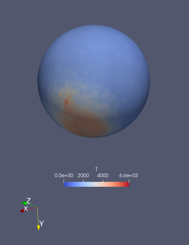
Fig 1. Temperature field (result from SPH model) at the start of simulation t=0 Myr
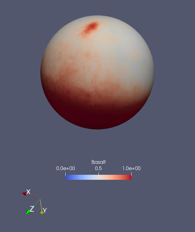
Fig 2. Compositional field at t=~500 Myr
[1] Watters, T., McGovern, P., & Irwin III, R. (2007). Hemispheres Apart: The Crustal Dichotomy on Mars. Annual Review Of Earth And Planetary Sciences, 35(1), 621-652.
[2] Wieczorek, M., Broquet, A., McLennan, S., Rivoldini, A., Golombek, M., & Antonangeli, D. et al. (2022). InSight constraints on the global character of the Martian crust. Journal Of Geophysical Research: Planets. doi: 10.1029/2022je007298
[3] Taylor, S., & McLennan, S. (2009). Planetary crusts. Cambridge, UK: Cambridge University Press.
[4] Cheng, K.W., Tackley, P.J., Rozel, A.B., Golabek, G.J. (2021). Martian Dichotomy: Impact-induced Crustal Production in Mantle Convection Models, Abstract [DI35B-0023] presented at 2021 Fall Meeting, AGU, New Orleans, LA, 13-17 Dec.
[5] Emsenhuber, A., Jutzi, M., Benz, W. (2018). SPH calculations of Mars-scale collisions: The role of the equation of state, material rheologies, and numerical effects. Icarus, 301, 247-257
[6] Tackley, P. (2008). Modelling compressible mantle convection with large viscosity contrasts in a three-dimensional spherical shell using the yin-yang grid. Physics Of The Earth And Planetary Interiors, 171(1-4), 7-18.
How to cite: Cheng, K. W., Rozel, A., Ballantyne, H., Jutzi, M., Golabek, G., and Tackley, P.: Martian crustal dichotomy formation and its effect on volcanisms: mantle convection models, Europlanet Science Congress 2022, Granada, Spain, 18–23 Sep 2022, EPSC2022-1045, https://doi.org/10.5194/epsc2022-1045, 2022.
Introduction. Oxia Planum is the selected landing site of the ExoMars mission [1]. A drilling system is installed on the ExoMars rover, able to analyze down two meters in the subsurface of Mars. Among the scientific objectives of the ExoMars mission, the searching of the organics or volatiles species plays an important role. The Ma_Miss spectrometer (Mars Multispectral Imager for Subsurface) [2] will investigate the borehole generated by the drill and it will be able to characterize and map the presence of possible ices. In this work we developed a numerical model to predict the subsurface temperatures after the heat released by the drilling operations. The increase in temperature due to the drilling operations, in fact, could affect the survivor of the volatile species [3]. Here we report the results about subsurface temperature of Oxia Planum.
Numerical modeling
We developed a numerical modeling to predict the subsurface temperature of Oxia Planum. In the subsurface we solve the classical heat equation [3]:

where ρ is the density, c p the specific heat, K the thermal conductivity and T the temperature. Heat transfer occurs only by conduction since convection is negligible due to the small temperature gradients involved as well as the characteristic size of the sample. At the top we imposed a radiation boundary condition. In order to take into account the heat released by the drilling operations we imposed a frictional heating flux on the sides “in contact” with the drill (the lateral sides of the borehole of Fig.1). This flux is defined by the equation [3]:

where η is the coefficient of friction, Fn the thrust, ω the rotational velocity, r the radius of the hole and h the height of the domain of integration (in our case 50 cm).
The parameters adopted in this work are F n = 300 N, rpm = 30 or 60, η = 0.3 or 0.9, tip density = 3500 kg m-3, tip thermal conductivity = 540 W m-1K-1, tip specific heat = 790 J kg-1K-1 and a drilling window of 90 min, characterized by 30 min in “on mode”, followed by 30 min in "off mode” and finally 30 min in “on mode”. The surface and subsurface of Oxia Planum is characterized by a thermal inertia of 650 TIU, with an initial temperature fixed to 200 K. Some assumptions are made: I) instantaneous drilling
(drill excavation is not modeled); 2) constant thrust; 3) constant rotational velocity.
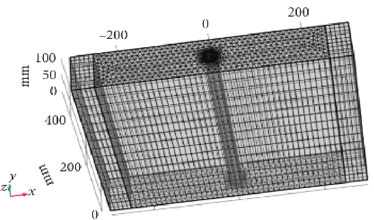
Fig.1: Geometry adopted in this work. The borehole of the drilling system is represented by the cylinder embedded in this domain of integration, with a radius of 13 mm (the thickness of the drill tip).
In Fig.2 we report an example of 1-D temperature profile at z=50 cm (the maximum depth of the borehole). In the x-axis we report the distance from the hole, where shadowed red rectangle identifies the drill (or equivalently the borehole). Top panel of Fig.2 is characterized by rpm=30 and η=0.3 while the bottom panel by rpm=30 and η = 0.9. From these plots we note a difference, in the maximum value after 90 minutes, of about 40 K in favour of the case with η=0.9. The increase in temperature due to the drilling operations, in case of η=0.9, respect the initial assumed value (200 K) is about 80 K. The initial value of 200 K is chosen since is close to the surface equilibrium temperature value for Mars. As in [4] we can calculate the lifetime of an ice spherical deposit of mass m0, with a radius equal to the radius of the drill tip. The relative loss of ice mass at time (t) after the deposit is raised the temperature T is:

where t is the time expressed in seconds. In this equation, Г represent the water rate emission, rp the radius of the tip and рice the density of the ice. By using the maximum sublimation rate, we obtain in case of rpm = 30 and η=0.3 a loss of about 60% of the initial mass, while in case η=0.9 of the loss is complete.

In Fig.2 we report an example of temperature internal profile after the heat released by the drilling operations. Both panels refer to rpm=30: top panel is characterized by η=0.3 while bottom panel by η=0.9.
Summary and Conclusions. We simulated the heat released by the drilling operations in different case of friction (η) and rotatonal speed (rpm) of the drill. We observed that in case of η=0.3 the maximum temperature increase at a depth of 50 cm is about 55 K (with rpm=30) and about 75 K (with rpm=60), while in case of η=0.9, the maximum temperature increase becomes 90 K (with rpm=30) and 130 K (with rpm=60) [3]. We also calculated the sublimation rate and the lifetime of a hypothetical spherical ice-rich deposit, with a radius equal to the size of the tip of the drill. We obtained that, after 90 minutes from the start of our simulations, in the coldest scenario (η=0.3 and rpm=30) the remaining initial mass is about the 60%, while in the other scenarios we have a complete loss of the mass [3]. Future improvements in the numerical model (e.g. a complete treatment of the diffusion of volatiles) as well as validation with laboratory experiments will be made.
Acknowledgments. This work is funded and supported by the Italian Space Agency (ASI) [Grant ASI-INAF n. 2017-48-H.0].
References [1] Vago J.L. et al. 2017; [2] De Sanctis M.C. et al 2017; [3] Formisano M. et al. 2021; [4] Andreas E.L. 2007; [5] Coradini A. et al. 2001
How to cite: Formisano, M., De Sanctis, M. C., Federico, C., Magni, G., Altieri, F., Ammannito, E., De Angelis, S., Ferrari, M., and Frigeri, A.: Numerical modeling of subsurface temperatures of Oxia Planum, landing site of ExoMars mission, Europlanet Science Congress 2022, Granada, Spain, 18–23 Sep 2022, EPSC2022-839, https://doi.org/10.5194/epsc2022-839, 2022.
Fully dynamical 3D simulations that self-consistently model the evolution of mantle flow are routinely used to investigate the thermal history of the interior of rocky planets, and through their nature, they can address both global and local observations in regions of interest. Over the past years, models of the thermal evolution of Mars have been combined with crustal thickness variations derived from gravity and topography data, tidal deformation models, and calculations of the seismic velocities and seismogenic layer thickness to estimate the present-day seismicity.
Recent data from the InSight mission about the crustal thickness, upper mantle structure, and core size provide the most direct constraints on the interior structure of Mars. Here we use InSight’s estimates in addition to constraints from tidal deformation, elastic lithosphere thickness, and recent volcanic activity to model the thermal history and present-day state of the interior of Mars.
Similar to previous studies (Plesa et al., 2016, 2018), the geodynamical simulations include crustal thickness variations (Fig. 1a). We use the most recent global crustal thickness models of Mars (Wieczorek et al., 2022) that are derived from gravity and topography data and constrained by crustal thickness estimates at the InSight landing site from seismic observations (Knapmeyer-Endrun et al., 2021; Wieczorek et al., 2022).
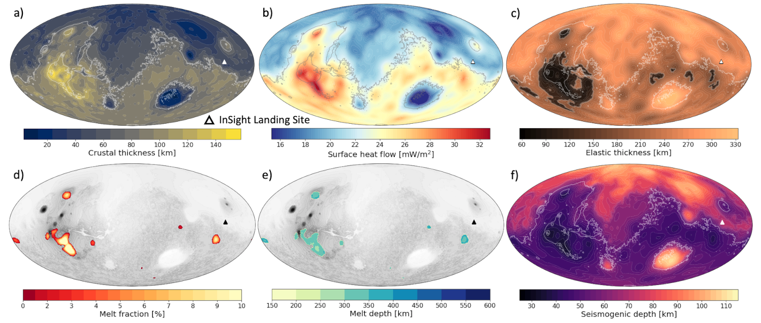
Fig. 1: a) crustal thickness model derived from gravity and topography data and anchored by the crustal thickness at InSight location; b) corresponding heat flow and c) elastic thickness variations at present day; d) average melt fraction and e) average melt zone depth at present day; f) seismogenic layer thickness computed using the 573 K isotherm.
The present-day thermal state in the 3D geodynamical models is obtained by running the entire thermal evolution of Mars. The models assume that 55 to 70% of the bulk amount of heat producing elements are stored in the crust as suggested by Knapmeyer-Endrun et al. (2021) in order to avoid wide-spread melting in the interior of Mars at present day. The strong crustal enrichment, and thus a mantle depleted in heat sources, leads to an average present-day lithospheric thickness of about 500 km in good agreement with the thermal lithosphere thickness estimated from the analysis of seismic events (Khan et al., 2021; Duran et al., 2022).
Our models show that crustal thickness variations have a first order effect on the temperature distribution in the shallow mantle. Thus, the patterns of the surface heat flow and elastic lithosphere thickness at present day correlate with the crustal thickness variations (Fig. 1b,c). The present-day elastic lithosphere thickness at the north pole of Mars is one of the strongest constraints for thermal evolution models and indicates that the mantle contains less than 45% of the total heat production and/or that the polar cap has not yet reached elastic equilibrium (Broquet et al., 2020).
The radius of the core in our models has been set to 1850 km, a value that lies well within the current core radius estimates (Stähler et al., 2021). Such a large core prevents the stability of an endothermic phase transition from wadsleyite/ringwoodite to bridgmanite that was previously proposed to explain the formation of the martian crustal thickness dichotomy and Tharsis through a low degree convection pattern (Harder & Christensen, 1996, Breuer et al., 1998). Current models show a mantle characterized by several mantle plumes distributed throughout the mantle. During the evolution, strong mantle plumes that produce melt up to recent times become focused in regions covered by a thick crust, in particular in the Tharsis province (Fig. 1d,e).
We compute the tidal deformation using the interior structure and present-day thermal state from the geodynamic models. For the tidal deformation calculations, we use a semi-analytical model based on the normal mode theory for radially stratified viscoelastic bodies (Sabadini & Vermeersen, 2004) and choose an Andrade rheology. Results show that thermal evolution models with a large core and a dry mantle viscosity can match the latest tidal deformation estimates determined from radio tracking measurements from Mars Odyssey, Mars Reconnaissance Orbiter, and Mars Global Surveyor (Konopliv et al., 2020).
Similar to the study of Plesa et al. (2021), we compute the seismic velocities in the entire 3D thermal evolution model. We use the mantle compositions of Taylor (2013), Yoshizaki & McDonough (2020), and include the most recent composition of Khan et al. (2022). Independent of the assumed compositional model, seismic velocity variations show a pattern similar to that of the crustal thickness and these variations can extend to depths of 400 km or deeper for models with a thick lithosphere.
Our models can be used to estimate the seismogenic layer thickness and the present-day seismicity of Mars and to compare the results with the recent estimates from InSight (Banerdt et al. 2020). Using isotherms of 573 K and 1073 K that have been suggested to mark the base of the seismogenic layer (Knapmeyer et al., 2006 and references therein), we calculate the thickness of the seismogenic zone at each location on Mars (Fig. 1f) and estimate the present-day seismicity. The seismogenic layer thickness follows crustal thickness variations and could be used to discriminate between geodynamic models, if the source depth and location of seismic events is known. The present-day seismicity calculated from the geodynamic models that use the crustal thickness and core size estimates from InSight is compatible with the values derived from InSight's seismic data.
Future models need to analyze in greater detail the consequences of the large present-day elastic lithosphere thickness at the north pole of Mars from recent estimates on the present-day thermal state. Geodynamic models combined with seismic waves propagation calculations need to investigate the effects of spatial variations of seismic velocities in the mantle and lithosphere, and future studies are necessary to test the spatial distribution of seismicity by comparing model predictions to observations.
How to cite: Plesa, A.-C., Wieczorek, M., Knapmeyer, M., Rivoldini, A., Walterova, M., and Breuer, D.: Interior Dynamics and Thermal Evolution of Mars – a Geodynamic Perspective, Europlanet Science Congress 2022, Granada, Spain, 18–23 Sep 2022, EPSC2022-1218, https://doi.org/10.5194/epsc2022-1218, 2022.
Introduction:
Pit craters are peculiar depressions found in almost every terrestrial body of the Solar System [1]–[4]. Morphologically characterized by circular to elliptical shapes, flat rim and no ejecta blankets. Often found aligned to form a pit chain, or even coalesced with other pits. Depending on their morphology and type of alignemt (e.g. sinuous or straight in presence of faults) their origin may be attributed to either tectonic or to the collapse of a lava tube [2]. On the other hand, atypical pit craters can be found isolated with no major additional surface morphological expressions. In this work, we present a morphometric analysis of one of the atypical pit craters found on the flank of Pavonis Mons. The pit central coordinates are Lon -110.80 Lat 0.33
Data:
We used a single stereo pair, ESP_033935_1805 - ESP_041900_1805, acquired by the High Resolution and Imaging Science Experiment (HiRISE) [5]and downloaded from NASA ODE-PDS [6].
Morphometric analysis:
We created a high-resolution Digital Elevation Model (DEM) with a spatial resolution of 0.5 m/pixel, using a custom Jupyter Lab environment [7] to process the data with the Integrated Software for Imagers and Spectrometers (ISIS) [8] and the Ames Stereo Pipeline [9]. Finally, using QGIS v3.24, we performed the morphometric analysis, summarized in Table 1.
Within QGIS, we digitised the shape of the pit, contouring the rim on the orthoimage, where is clearly recognizible the extension of the pit, as shown in Figure 1.
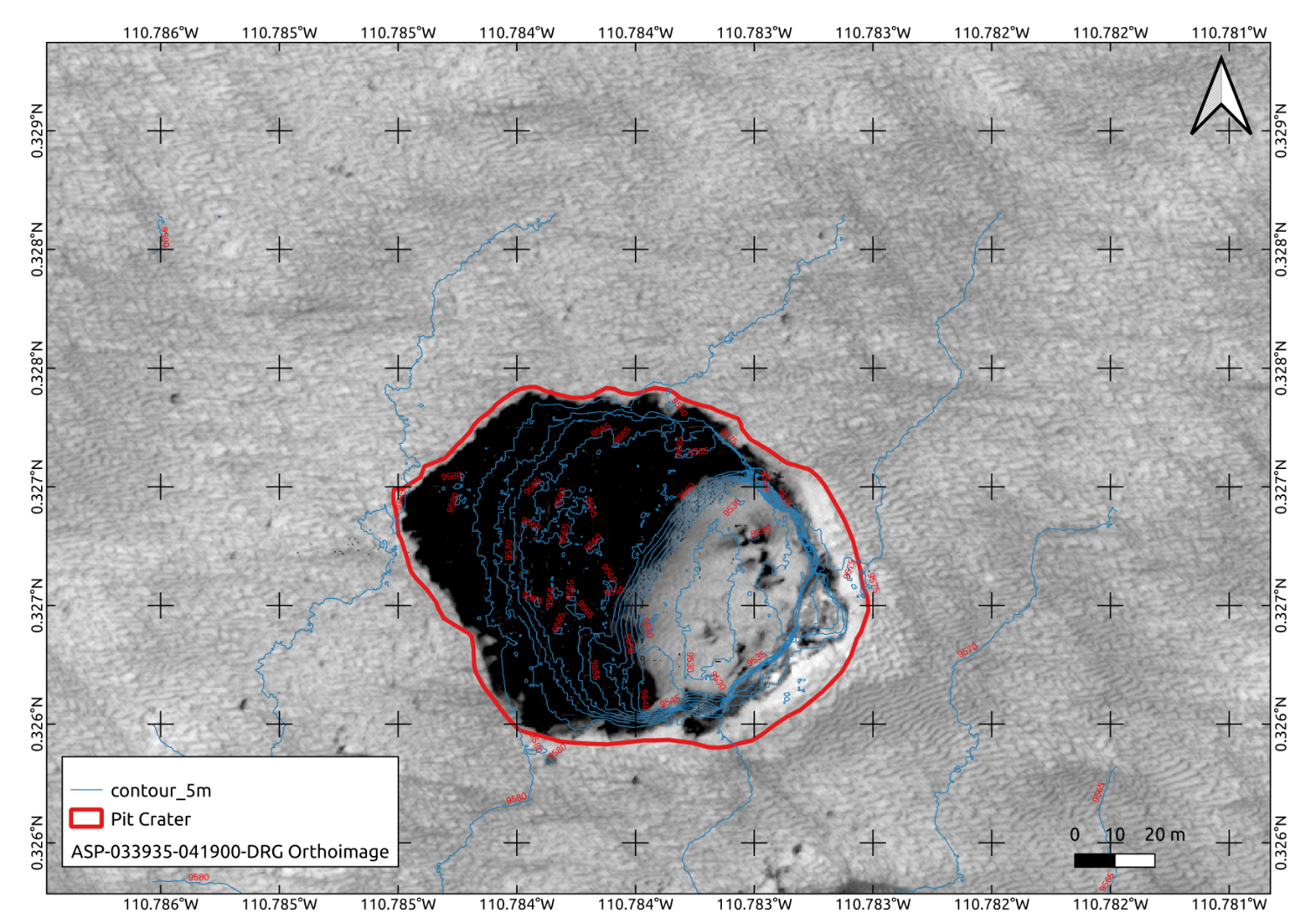
Figure 1. In red, the polygon of the pit, designed over the orthoimage.
Then we measured the semi-axis of the ellipse inscribing the shape of the pit and, finally, we used the plugin Volume Calculation Tool to compute the volume of the pit. We also computed elevation contour lines at 2 m interval. Figure 2 shows graphically the results of the analysis.
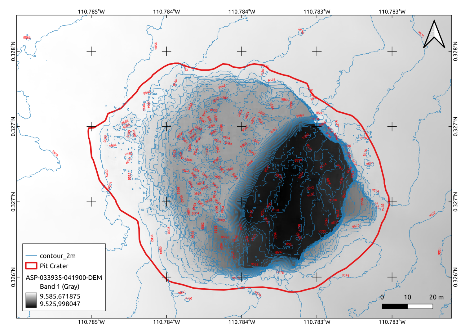
Figure 2. Map of the pit, showing the elevation in blue lines. The pit seems to have two main levels of collapse, an upper level with terraces on both sides, one less developed than the other, and the floor base level.
The area of the pit covers approximately 7978 m2, with a perimeter of 336 m. The edges of the enveloping hexagon have an average length of 56m. The bottom of the pit is at approx. 9525 m, while the rim has an average elevation of 9583 m, giving a height of ca. 60m. Analysis of the DEM shows two levels of collapse.The volume computation is underestimated due to the uncertainity of the left terrace. This terrace may be the results of the interpolation performed by the ASP algorithms due to the presence of hard shadows in the stereo pair. Considering that this left terrace cover almost half of the pit, we may infer that the estimated volume may be approximately double the measured volume. Further analysis, including shapes-from-shadows, may improve this result.
|
Parameter |
Value |
|
Volume |
~ 303.724 m3 measured, ~ 600 m3 estimated.
|
|
Area |
7978 m2 |
|
Perimeter |
336 m |
|
Average side length |
~ 56 m |
|
Average Max Elevation (RIM) |
~ 9583 m |
|
Min Elevation (bottom) |
~ 9525 m |
|
Maximum Depth |
~ 60 m |
|
Semi-Major axis |
~ 60 |
|
Semi-Minor axis |
~ 90 |
Table 1. Summary of the parameters of the Hexagonal Pit, retreived by analysing the high-resolution DEM.
As the last step, we imported the DEM as a terrain in Unreal Engine 5, to visualize it in simulated different light conditions, as shown in Figure 3.
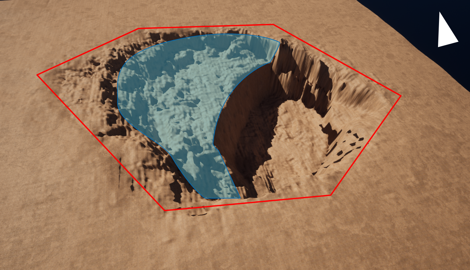
Figure 3. Pit DEM imported into Unreal Engine 5. The virtual sides of the hexagon are shown in red, while in cyan is highlighted the shadowed area in the stereo pair.
Conclusion:
The pit presented in this work has some unusual characteristics, its uncommon hexagonal shape, and the absence of connected secondary erosional mechanisms such as impact craters and pits could indicate the presence of structural elements that guided the rupture of the surface.
Funding:
This study is within the Europlanet 2024 RI, and it has received funding from the European Union’s Horizon 2020 research and innovation programme under grant agreement No. 871149.
References:
[1] D. Wyrick, D. A. Ferrill, A. P. Morris, S. L. Colton, and D. W. Sims, ‘Distribution, morphology, and origins of Martian pit crater chains’, J. Geophys. Res. Planets, vol. 109, no. E6, 2004, doi: 10.1029/2004JE002240.
[2] F. Sauro, R. Pozzobon, M. Massironi, P. D. Berardinis, T. Santagata, and J. D. Waele, ‘Lava tubes on Earth, Moon and Mars: A review on their size and morphology revealed by comparative planetology’, Earth-Sci. Rev., vol. 209, p. 103288, 2020, doi: https://doi.org/10.1016/j.earscirev.2020.103288.
[3] G. E. Cushing, ‘Mars Global Cave Candidate Catalog (MGC3)[abstract 3708]’, 2017.
[4] I. S. Hong, Y. Yi, J. Yu, and J. Haruyama, ‘3D modeling of lacus mortis pit crater with presumed interior tube structure’, J. Astron. Space Sci., vol. 32, no. 2, pp. 113–120, 2015, doi: 10.5140/JASS.2015.32.2.113.
[5] A. S. McEwen et al., ‘Mars Reconnaissance Orbiter’s High Resolution Imaging Science Experiment (HiRISE)’, J. Geophys. Res., vol. 112, no. E5, p. E05S02, May 2007, doi: 10.1029/2005JE002605.
[6] PDS Geosciences Nodes, ‘Orbital Data Explorer - Mars Holdings’. 2021. Accessed: Nov. 10, 2020. [Online]. Available: https://ode.rsl.wustl.edu/odeholdings/Mars_holdings.html
[7] G. Nodjoumi, C. Brandt, and A. P. Rossi, ‘Open-source planetary data processing environments based on jupyterhub and docker containers.’, p. 2, 2022.
[8] J. Laura et al., Integrated Software for Imagers and Spectrometers. Zenodo, 2021. doi: 10.5281/zenodo.5347823.
[9] R. Beyer, O. Alexandrov, and S. McMichael, NeoGeographyToolkit/StereoPipeline: NASA Ames Stereo Pipeline 2.6.1. Zenodo, 2018. doi: 10.5281/zenodo.1345235.
How to cite: Nodjoumi, G., Pozzobon, R., Sauro, F., and Rossi, A. P.: Morphometry of an hexagonal pit crater in Pavonis Mons, Mars, Europlanet Science Congress 2022, Granada, Spain, 18–23 Sep 2022, EPSC2022-1128, https://doi.org/10.5194/epsc2022-1128, 2022.
- Introduction
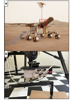
Figure 1: Rosalind Franklin rover . (a) CLUPI on the drill box (red rectangle, Image credit ESA/SEI-TJ). (b) CLUPI flight model representative (EM+) mounted in the stowed drill configuration, Image credit SEI.
Therefore, for this scientific goal, the objective is to reconstruct topographical and 3D data from the CLUPI data, using specific CLUPI operating configurations. This project is in collaboration with the Laboratoire d’Astrophysique de Marseille (LAM, France).
- 3D and stereo with CLUPI
CLUPI 8 configurations are linked to the drill box positions (Fig.2, Josset et al., 2017). In order to constrain the topographical data from the images acquired by CLUPI we will used the stereogrammetry method (Beyer et al., 2018). To perform that we need several images of the same geological target but with different stereo-angle (i.e. the angle between the target and CLUPI in the target repository (Fig.3)). CLUPI is a mono optics camera system. Thus, the different shots resulting in different stereo angles will come from the movement of the drill box and/or the rover itself. So, the main question of this project is how to define the optimal geometries parameters to obtain stereo images of the same target according to the 8 CLUPI operating configurations?
- Experimentation and preliminary result
In order to simulate the operation environment of CLUPI, we are using the EM+ flight model representative in the Space Exploration Institute CLUPI science operation lab based in Microcity, Neuchâtel, Switzerland. The CLUPI EM+ is adapted on a geometric drill simulator, corresponding to the ExoMars Rover mission (Josset et al., 2017). The objectives of this experimentation are to (1) recreate the CLUPI operating configurations, (2) vary parameters such as: the angle of incidence, the working distance and the CLUPI height relative to the ground; the illumination (studied in Marslabor, University of Basel; Bontognalli et al., 2021), and (3) derived the best geometrical position of the rover in order to reconstruct topographical data (Fig.3a).

Figure 2: CLUPI eight operational configurations. (a) On the platform, (b) geological environment survey, (c) Close-up outcrops observation, (d) drilling area observation, (e) drilling operation observation, (f) Drill hole and fines observation, (g) drilled core sample observation and (h) calibration: calibration target imaging. Images credit: ESA/SEI-TJ
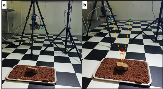
Figure 3: Experiment with the EM+. (a) Simulation of the second configuration. (b) Simulation of the second configuration after the calculated translation and rotation of the "rover", with a stereo angle (red) and the same working distance (yellow). The green and blue points correspond, respectively to the EM+ position before and after the translation/rotation.
- Illumination study (Basel University)
The total light and direction of incidence light plays an important role in allowing the identification of different rock textures, morphological features, and mineralogical distribution. The effect of different solar angles in relation to the target rock is studied with CLUPI analogue camera - Canon EOS M50. The most recent results show that to identify sedimentary structures, such as cracks, laminations and other morphological features in sedimentary rocks, the lower angle of 25° of direct light is preferable (sunset conditions on Mars, Fig.4a, c). In contrast, the distribution of the minerals within the rock, the incident/direct light shall be around 70° to the rock surface (mid-day conditions on Mars, Fig.4b,d).
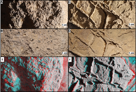
Figure 4. Close-up images in third configuration of basaltic tuff (A&B) and dry cracks in sedimentary rock (C&D) taken with Canon EOS M50 in Marslabor at University of Basel. (a) and (c) direct light of the angle 25 °. (b) and (d) direct light of an angle 70 °. Each to the rock surface. The total proportion of the light was 5:1 of direct and diffused light - 5000 LUX and 1000 LUX respectively, after Bontognali et al., 2021. With a working distance of 650 mm and camera angle of 11 °. (e) and (f) are anaglyph made from basaltic tuff (a) and (b) and dry cracks in sedimentary rock with the Canon, 25° light angle and a working distance of 760 mm.
- Stereo and 3D study (Space Exploration institute, Neuchâtel)
Currently, we succeed to define the optimal positions, with respect to configuration 2 and 3. For the configuration 2, the images with different stereo angle come from a translation then a rotation of the rover (Fig.3). The stereo images from the configuration 3 come from the different drill positions. In these two cases, the calculated positions make it possible to keep the same working distance despite the movements. This point is particularly important to reconstruct the topography rigorously.
We also reconstruct the firsts 3D anaglyphs based on the third configuration (Fig.4e, f and Fig.5).
- Conclusion and acknowledgment:
These study and related experiments consisting in varying the following parameters: the angle of incidence, the illumination, the working distance, the height relative to the ground, allows to faithfully reproduce the CLUPI operations configurations. These first results are promising since we succeed to define the geometrical parameters optimally to derive the topography data for 2 configurations. We will continue to investigate on the other configurations to quantify the rock morphometry recorded in the rock matrix. These steps are essential to significantly increase the science exploitation of CLUPI. The authors want to acknowledge the Swiss National Science Foundation (Subside 200021_197293/1), who is funding this project with the support of the Swiss Space Office and ESA Prodex.
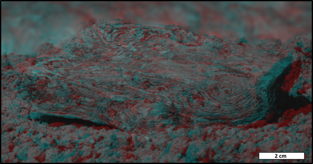
Figure 5: Anaglyph of a stromatolite performed in the SEI/Lab using CLUPI Flight Model Representative in the third configuration with a working distance of 1 m and a stereo angle of 10°. Images credit: SEI.
References:
Beyer, R. A., Alexandrov, O., & McMichael, S. 2018, Earth and Space Science, 5, 537– 548.
Bontognali, T., Meister, Y., Kuhn, B., et al., 2021, Planetary and Space Science, 208, 2021, 105355
Bouquety, A., Sejourné, A., Costard, F., et al., 2019, Geomorphology, 334, 91
Bouquety, A., Sejourné, A., Costard, F., et al., 2020, Geomorphology, 350, 106858
Bouquety, A., Jorda, L., Groussin, O., et al. 2021, Astronomy & Astrophysics,649, A82
Bouquety, A.,Groussin, O., Jorda, L., et al. 2022, Astronomy & Astrophysics: https://doi.org/10.1051/0004-6361/202142417
Josset, J.-L., Westall, F., Hofmann, et al., 2017. Astrobiology 17, 595–611.
How to cite: Bouquety, A., Jorda, L., Ligeza, G., Fayon, L., Narbey, R., Josset, T., Bontognali, T., Kuhn, N., and Josset, J.-L.: Preparation of ExoMars mission. Preliminary study for 3D and stereo science operations by using CLUPI flight model representative: Toward a morphometrical analysis, Europlanet Science Congress 2022, Granada, Spain, 18–23 Sep 2022, EPSC2022-1255, https://doi.org/10.5194/epsc2022-1255, 2022.
Introduction: ExoMars rover Rosalind Franklin will search for traces of past or present life potentially preserved in the designated landing site Oxia Planum [1]. Oxia is located in the western part of Arabia Terra, where geology shows evidence of a past long-lived liquid water body [2]. This clay-bearing plain is overlapped by deltaic system material provided by channels of Coogoon Valles. Spectral detections underlie the possible presence of Fe-rich phyllosilicate (for example vermiculite) and Mg-rich phyllosilicate (for example saponite) mixed with a variable amount of olivine. A mafic coating-resistant unit seems to be present [3,4,5].
Many minerals are expected to be analyzed by the Ma_MISS (Mars Multispectral Imager for Subsurface Studies) instrument at the landing site. The drill is also made up of three extensible 50 cm-long rods. The instrument is a VNIR (0.4–2.3 µm) miniaturized spectrometer in-stalled into the rover drill’s tip. It will acquire borehole spectral images in situ to study the subsurface mineralogy up to 2 m depth with a spatial resolution of 120 µm for looking at organics traces. Ma_MISS is composed of the Optical Head with fibres into the tip and the other fibres in the rods, while the spectrometer and the electronic are outside on the drill box. The sapphire window in the main rod allows the 5W light to illuminate inside the borehole and the reflected signal to be acquired by the spectrometer. The light illuminates a 1 mm diameter spot at ~0.6 mm focal distance. Thanks to drill rotation and vertical movement, Ma_MISS can collect several points to reconstruct a complete borehole image [1].
Laboratory breadboard: Drill for Analogues and Visible-Infrared Spectrometer (DAVIS) is the recent laboratory setup consisting of Laboratory Drill (DAVIS-LD) and Ma_MISS Optical Tool (DAVIS-MOT) (Figure 1). The first one (LD) is the replica of the rover drill except for the spectral acquisition system. The vertical motion is actuated by a hand lever to drill a hole in the rock samples. The motor unit is the same as the flight model but the controller is a commercial EC motor, which control the rotational speed (50 rpm) [6]. The second one (MOT) comprises a 75 cm-long and 25.4 mm-diameter rod, 5W lamp, Sapphire window, Optical Head, and an optical fibre. It is the copy of rover Ma_MISS except for the drilling ability. In this case, rover spectrometer is replaced with two Avantes VIS-NIR spectrometers. The Optical Head fibre is connected with the Avantes fibre through a mini-Avim connector. Being a replica of Ma_MISS, the light spot has 1 mm diameter at ~0.6 mm focal distance and the spatial resolution is 120 µm. It acquire in two different configurations: 1) Slab or powder samples are hosted in a vertical three-axis sample-holder and 2) manual motion of the rod to enter in the sample borehole [7].


Figure 1 – a) Ma_MISS Optical Tool (DAVIS-MOT) and b) Laboratory Drill (DAVIS-LD).
Martian Analogue sample: The Martian analogue denominated CAP-1 was collected during a geological survey of the Institute for Space Astrophysics and Planetology (IAPS), in October 2021. It was gathered in 120 cm-depth excavated trench in the area of Capalbio (Tuscany, Italy). It is a Pleistocene metasedimentary rock subjected to hydrothermal alteration/weathering (Figure 2). This brownish siltstone/mudstone is a quite compact rock in dry conditions and brittle in wet conditions. Inside it, there are a few discoidal, sub-angular grains with a diameter higher than 2 mm and different colors (black, reddish, and white), and low sphericity. Grains are not-oriented, except for black Manganese aggregates, which form thin veins with a diameter of about 2-5 mm. Other grains are white rectangular precipitations of Al-bearing clay (kaolinite) and reddish irregular aggregates formed by iron oxide (hematite). The brownish fine-grained (granulometry in the order of silt-clay) matrix has medium porosity, without cement. It lacks stratification and it shows possible alteration due to iron oxidation. CAP-1 is well-sorted, texturally and compositionally mature. The mineral assemblage of the CAP-1 sample is constituted of Mg/Fe smectite, kaolinite, illite, quartz, and minor calcite. It can contain some part of organic material based on analysis of similar soil in the area, but no detectable fossil evidence is found inside.
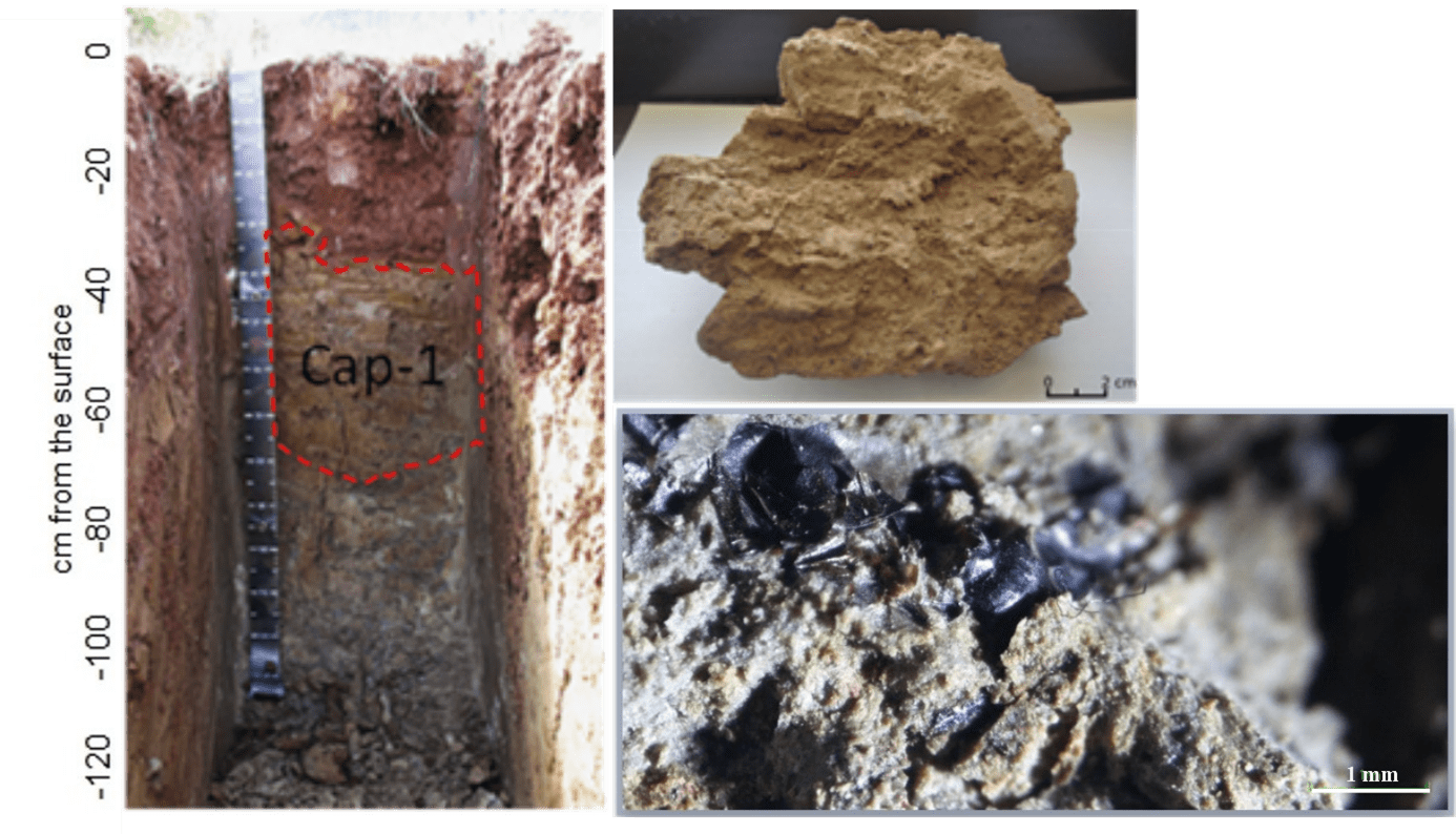
Figure 2 – a) Outcrop where CAP-1 is extracted (sampling depth 30-75 cm); b) Sample Capalbio CAP-1; c) Details of CAP-1 taken under a microscope: Mn aggregates.
Discussion and conclusions: Some preliminary acquisitions are taken using the DAVIS-MOT, as we can see in Figure 3. We acquire 3 random points on a planar surface of the sample. After that, raw data of spectra are smoothed and merged between 1075 and 1140 nm (the AVANTES spectrometer has two different detectors and the acquisitions are made for the VIS and IR in two steps). Resampling is done in 364 points between 400 and 2300 nm. Spectra show characteristic absorption bands of water at 1.4 and 1.9 µm, well-shaped absorption bands at 0.95 and 2.2 µm associated with iron transition and Al-OH bond respectively. A deep spectral analysis will be done after the new laboratory acquisition of this sample.
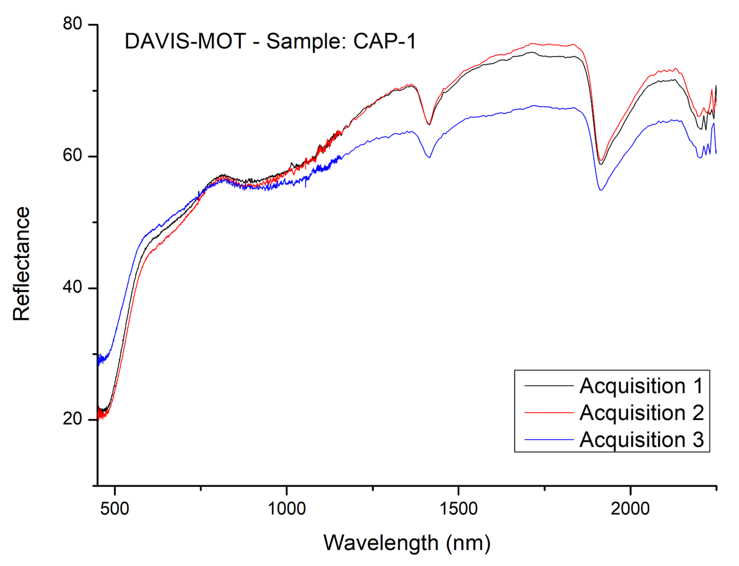
Figure 3 – VIS-NIR CAP-1 spectra acquired by DAVIS-MOT.
Acknowledgments: This work is supported by the Italian Space Agency (ASI) grant ASI-INAF n. 2017-412-H.0. Ma_MISS is funded by ASI and INAF.
References: [1] De Sanctis, M. C. et al. (2017) Astrobiology, 17(6–7), doi: 10.1089/ast.2016.1541; [2] Davis, J. M. et al. (2016) Geology, 44(10), doi: 10.1130/G38247.1; [3] Quantin-Nataf, C. et al. (2021) Astrobiology, 21(3), doi: 10.1089/ast.2019.2191; [4] Mandon, L. et al. (2021) Astrobiology, 21(4), doi: 10.1089/ast.2020.2292; [5] Brossier, J. (2022) Icarus, accepted pending revisions; [6] Rossi, L. et al. (2022) LPSC 53, Abstract #1353, [7] De Angelis, S et al. (2022) LPSC 53, Abstract #1796.
How to cite: Costa, N., Ferrari, M., Frigeri, A., De Sanctis, M. C., De Angelis, S., Ragazzo, A. V., Altieri, F., Ammannito, E., Apuzzo, A., Rossi, L., and Formisano, M.: Importance of spectral acquisition of a Martian analogue with DAVIS breadboard, Europlanet Science Congress 2022, Granada, Spain, 18–23 Sep 2022, EPSC2022-165, https://doi.org/10.5194/epsc2022-165, 2022.
1. Introduction
Plagioclase feldspar (Plg) is a common mineral in terrestrial rocks. It is a solid solution between a Ca-rich (anorthite) and a Na-rich (albite) endmember, and it is most commonly classified based on its anorthite (An) content. Powders of anorthite-rich Plg were previously studied using reflectance spectroscopy in the visible near-infrared (VNIR) range [1]. They showed that Plg display a band centered around 1.3µm due to Fe2+ substitutions, and that the position of this absorption band is a function of the An content.
Other studies have investigated mixture of binary powders and showed that the Plg spectral signature is no longer visible when 10%, or more, of mafic minerals are added [2, 3]. According to these studies, a minimum of 90% of Plg are necessary in the rock composition for its spectral signature to be visible on the average spectrum of the rock. A more recent study, mixing large Plg and pyroxene grains [4], showed that at least 50% of mafic minerals are needed to mask the Plg spectral signature.
Therefore, in addition to the An content, the size of the grains and the associated minerals influence the spectral signature of Plg. Thus, the analysis of whole rocks, and not powders, appears to be more relevant as a comparison with remote sensing analysis of planetary surfaces.
The present study seeks to understand when Plg signatures are detectable, and how the Plg absorption band is affected by the nature of the host rock. In other words, does the spectral signature of Plg differ from one rock type to another, and if so, can a reflectance spectrum in VNIR be associated with a specific feldspathic rock type?
2. Method
We combined petrological and spectral laboratory analyses of five terrestrial rock samples that contain Plg: an anorthosite (NM6), a granite (NJ11), two porphyritic basalts (NR1 and NR2) and a dacite (NJ2) (Figure 1).
Firstly, reflectance spectroscopy measurements were carried out on the macroscopic samples using an ASD Fieldspec 4 point-spectrometer. The instrument operates in three different wavelength ranges: VNIR (0.35 – 1 µm), SWIR 1 (1.001 – 1.801 µm), and SWIR 2 (1.801 – 2.5 µm), with a spectral resolution between 3 and 8 nm.
All resulting spectra (Figure 2) have an absorption band centered around 1.3µm with broad shoulders located around 0.8µm and 1.7µm. In order to accurately determine if this band is related to Plg in the rocks, additional analyses were performed.
A petrographic study of each sample mineralogy (Figure 1) was carried out using an optical microscope as shown for sample NR1 in Figure 3.
The use of hyperspectral cameras made it possible to further determine the spectral signature of each grain contained in these rocks (Figure 1). Hyperspectral cubes were acquired with the HySpex VNIR-3000-N and SWIR-640 cameras that acquire high-resolution data respectively from 0.4µm to 1µm, and from 0.96µm to 2.5µm, at a distance of 30cm from the sample. The resulting pixel size is about 29 µm in the VNIR, and 130 µm in the SWIR. The hyperspectral cubes are converted to reflectance using a reference target, and then analyzed with the ENVI software to classify the image pixels according to their spectral signature. Therefore, the different minerals in the rocks, which are often on a millimeter scale, are grouped into different classes. The statistics give the mean spectrum of each class, and therefore each mineral group (Figure 4).
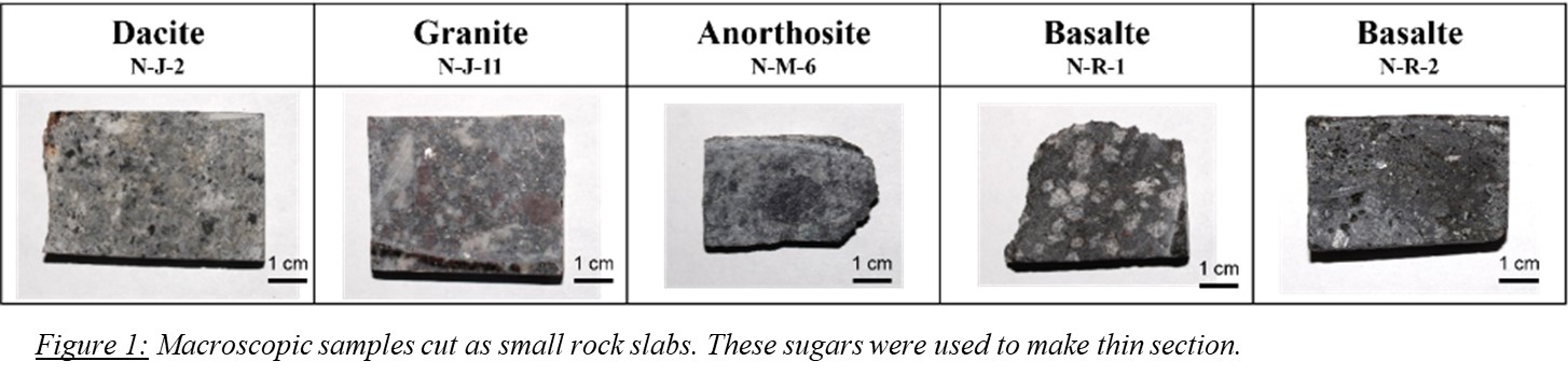

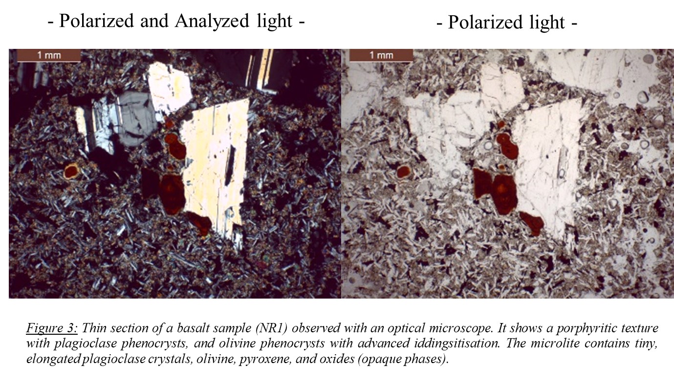
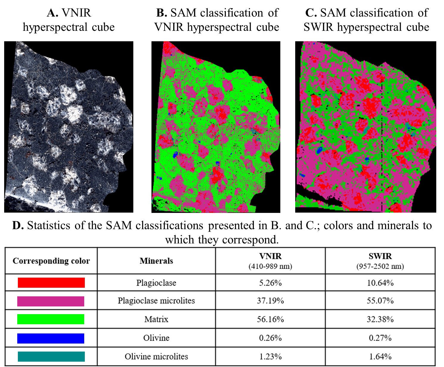
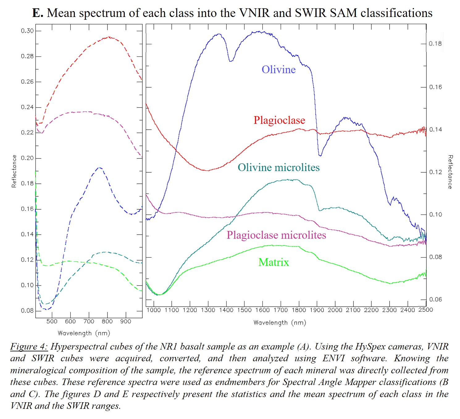
3. Results and Discussion
For each sample, the mineralogical composition (Figure 3) and spectral signature of each mineral (Figure 4) are determined. We observe that only Plg has an absorption band centered at 1.3µm with broad shoulders at 0.8 and 1.7µm. In conclusion, this same absorption band, that we see on the average spectrum of the rock (Figure 2), is the spectral signature of Plg. However, it should also be noted that in the matrix of Figure 4, composed of Plg and iddingsitized olivine, this band is no longer visible. This is also the case for the other samples: some minerals can mask the spectral signature of Plg by overlaying or attenuating its absorption band.
Looking at the reflectance spectra (Figure 2), the position of the band seems to vary. It is centered around 1.2µm for dacite (NJ2) and granite (NJ11), around 1.25µm for basalts (NR1 and NR2), and 1.3µm for anorthosite (NM6). However, one must be careful with the interpretation: this shape might be related to the Plg chemical composition, but also the grain size, and the presence of other minerals contributing to the average rock spectra.
Our study, therefore, shows that it is indeed possible to detect the presence of Plg in a whole feldspathic rock, even though it does not contain 90% of feldspar, and regardless of its nature (e.g., sample NR1 shown in Figure 4 contains ~66% of Plg).
These results can be applied to the study of feldspathic rocks at the surface of rocky planets and more precisely of Mars. Indeed, recent detections of Plg [5, 6, 7] were made using the CRISM instrument (MRO) at the surface of Mars. The interpretation of these signatures, in terms of lithologies, is still under discussion given the variety of feldspathic rocks containing plagioclase [4, 5, 6, 7, 8] that exhibit the typical Plg absorption band. The construction of a reference library acquired on macroscopic rock fragments that we undertook should lead to a more accurate interpretation of Martian detections.
4. References
[1] J.B. Adams an L.H. Goullaud (1978). LPSC Conference, 9th, 3, 2901-2909 (A79-39253 16-91).
[2] D.A. Crown and C.M Pieter (1987). Icarus, 72(3), 492-506.
[3] L.C. Cheek et al. (2014). American Mineralogist, 99(10), 1871-1892.
[4] A.D. Rogers et H. Nekvasil (2015). Geophy.Res.Lett., 42, 2619-2626.
[5] J.J. Wray et al. (2013). Nature Geoscience, 6, 1013-1017.
[6] J. Carter et Poulet (2013). Nature Geoscience, 6, 1008–1012.
[7] J. Flahaut et al. (2020). EGU General Assembly (EGU2020-13377).
[8] A.D. Rogers et W.H. Farrand (2022). Icarus, 376, 114883.
How to cite: Barthez, M., Flahaut, J., Guitreau, M., Pik, R., and Ito, G.: Reflectance spectroscopy and optical microscopy laboratory analyses of terrestrial feldspathic rocks as analogs to Mars, Europlanet Science Congress 2022, Granada, Spain, 18–23 Sep 2022, EPSC2022-467, https://doi.org/10.5194/epsc2022-467, 2022.
In partial melt zones, incompatible elements like the heat producing elements (HPE) K, Th, and U are redistributed from the solid to liquid material. If the melt is in an area where it is buoyant, it transports the incompatible elements towards the surface and leaves a depleted upper mantle area behind. Partition coefficients can act as a measure for the amount of the redistributed elements. They are highly sensitive to temperature, pressure, and composition and can change by multiple orders of magnitude along the peridotite solidus from 0-15 GPa (Fig. 1, Schmidt and Noack, 2021). However, since there is a lack of high-pressure models and experimental data, partition coefficients in mantle evolution models were generally taken as constant values.
Clinopyroxene is a common mantle material which takes up most trace elements and is therefore highly relevant for redistribution processes. Also, compared to other minerals that can be found in the upper mantle of Mars and Earth, clinopyroxene undergoes the largest changes of partition coefficients with changes in temperature and pressure. In clinopyroxene, sodium acts as a compatible element with partitioning behaviors similar to incompatible trace elements, which is why it can be used as a reference for modelling other trace elements’ partition coefficients. In this study, we take the parameterization for the partitioning of sodium of Schmidt and Noack (2021) and calculate partition coefficients for HPE at local P-T conditions. This parameterization is derived from a thermodynamic model (Fig. 1) based on Blundy et al (1995) and valid for pressures up to 12 GPa. We apply these calculated partition coefficients to a 1D interior evolution model for Mars and compare the resulting HPE enrichments to the ones obtained with models using constant partition coefficients for variable initial conditions. By doing so, we can compare data obtained from Mars missions to our modelled approach and subsequently constrain the influence the varied parameters and the partitioning model have on the thermal evolution of Mars.
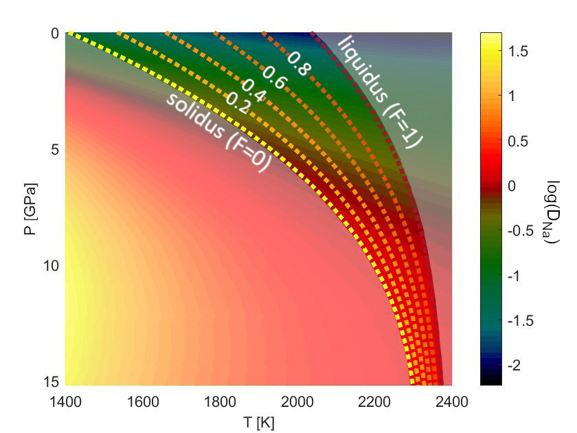
Fig. 1: Thermodynamic model for sodium partitioning in clinopyroxene/melt. Along the peridotite solidus,
the partition coefficients vary up to two orders of magnitude (Schmidt and Noack, 2021).
Schmidt, J.M. and Noack, L. (2021): Clinopyroxene/Melt Partitioning: Models for Higher Upper Mantle Pressures Applied to Sodium and Potassium, SysMea, 13(3&4), 125-136.
Blundy, J. et al. (1995): Sodium partitioning between clinopyroxene and silicate melts, J. Geophys. Res., 100, 15501-15515.
How to cite: Schmidt, J. M. and Noack, L.: Application of a P-T dependent partition coefficient model to a 1D thermal evolution code of Mars, Europlanet Science Congress 2022, Granada, Spain, 18–23 Sep 2022, EPSC2022-587, https://doi.org/10.5194/epsc2022-587, 2022.
Introduction: On Earth, sharp drops in temperature can cause ground cemented by ice to contract, forming surficial cracks (Figure 1a) that can join to form polygonal patterns. These polygons show no elevation difference between their margins and centres, and are called here flat-centred polygons (FCPs). Water and/or sand [1, 2, 3] can infill the troughs and freeze, forming ice or sand wedges. These grow seasonally, uplifting polygon margins above the centres, forming low-centred polygons (LCPs). When wedges degrade, the elevation of the margins decreases below that of the centre, forming high-centred polygons (HCPs).
The martian mid-latitudes exhibit similar polygons (Figure 1b), currently thought to form by ground thermal-contraction [4]. Whereas debate ensues over the nature of trough infill, recent work provided evidence for ice wedges in Utopia Planitia [5] – with implications for liquid water stability and subsurface water ice availability.
Here we study variations in polygon distribution/morphology in relationship with different geological units in UP (Figure 2) and Arcadia Planitia (AP; Figure 3), where polygonised units have been reported [6]. Our study seeks to understand: 1. how the substrate nature favoured/inhibited the formation and/or preservation of ground ice, and 2. whether polygon characteristics (e.g. morphology, spatial density) can give insights into geological properties of their substrate.
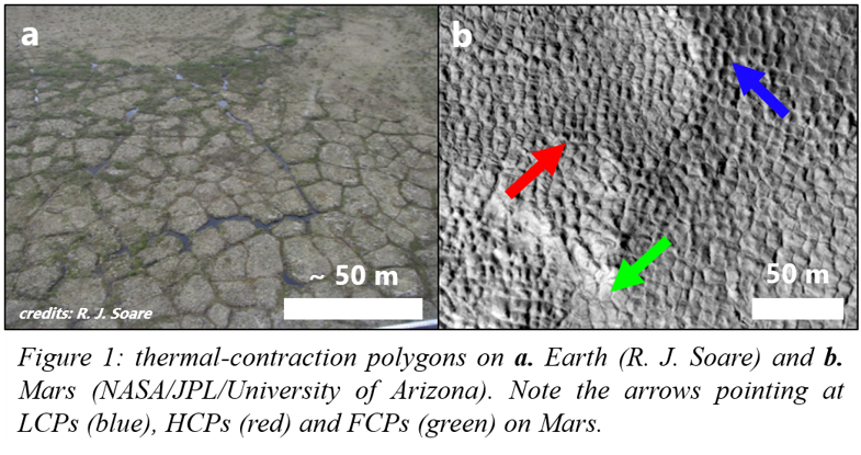
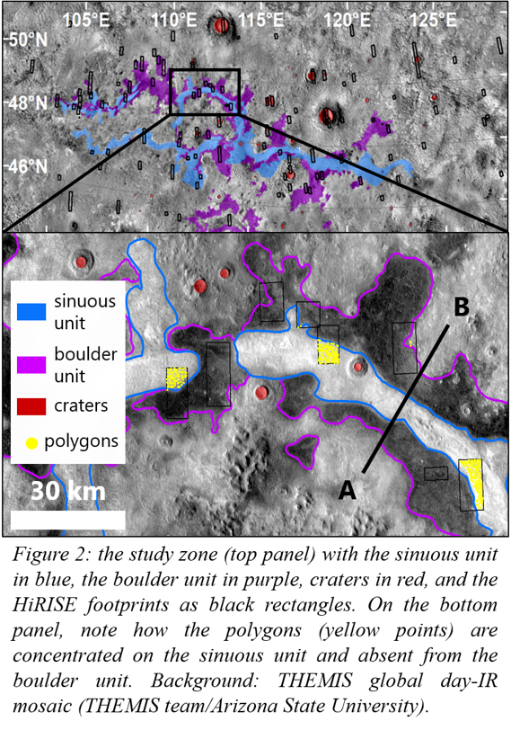
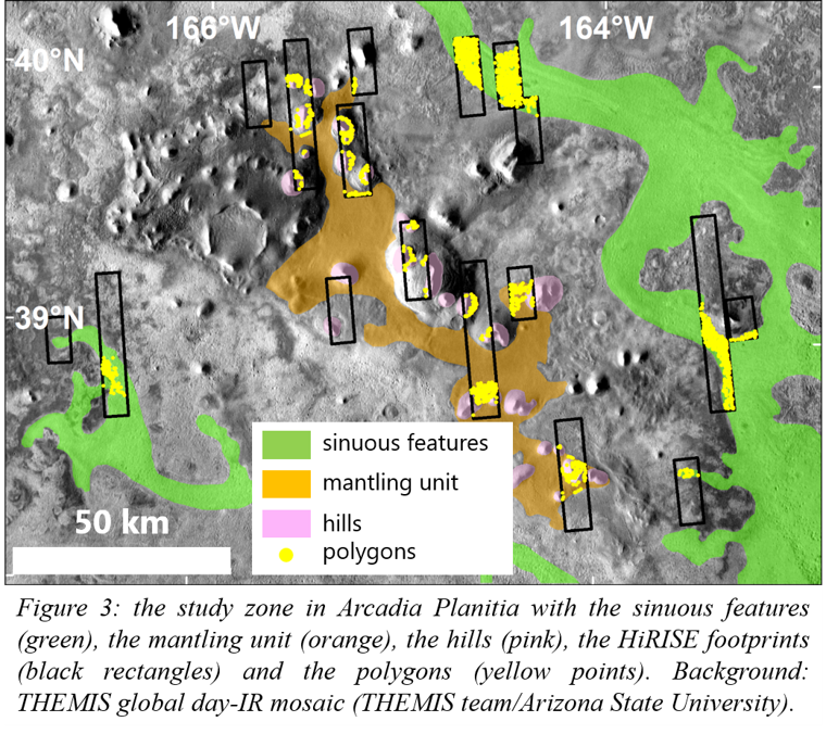
Methods: In UP (Figure 2a) we mapped polygons (5-25 m scale) on 104 images from the High-Resolution Imaging Experiment (HiRISE, 25-50 cm/pixel) – 55 from [5] and 49 new ones. We used a grid-based mapping approach [7]: we gridded images into 500x500 m squares, and in each square the presence of a given polygon type was noted when at least five specimens were present. We mapped the extent of three units: a sinuous unit, a boulder unit, and craters (Figure 2) with imagery from the Thermal Emission Imaging System (THEMIS), the Context Camera (CTX) and HiRISE. We also produced a topographic cross-section of contacts between the sinuous and the boulder units (Figure 2b) with data from the Mars Orbital Laser Altimeter (MOLA).
For each unit we calculated three parameters: 1. the percentage of polygonised squares (%pol), 2. the percentage of polygonised squares containing solely FCPs (%FCPs), and 3. the ratio number of squares containing LCPs / number of squares containing HCPs (LCP/HCP). We suggest that these parameters reflect properties of the substrate: 1. its cementation by ice, 2. its capacity to grow ice wedges (i.e. massive ground ice), and 3. its capacity to preserve ground ice.
We used the same approach on 18 HiRISE images in AP, where we mapped the extent of three units based on [6]: hills, a mantling unit, and sinuous features.
Results: We display and compare results for each unit in Table 1. In UP, topography and cross-section data (Figures 2b & 4) show that the boulder unit is at a lower elevation than the sinuous unit and also the surrounding terrains. In AP, hills exhibit FCPs around their central mound (Figure 5a); sinuous features bear FCPs, HCPs and what we interpret as degraded HCPs (Figure 5b); and the mantling unit bears few polygons, but is mostly covered in extensive brain terrain and linear ridges [6] (Figure 5c).
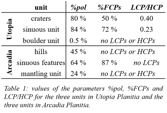
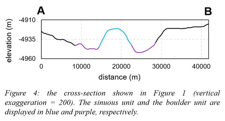
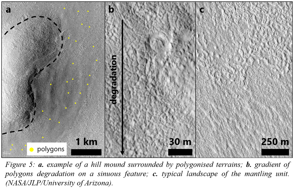
Discussion:
Utopia Planitia: The material infilling craters is highly polygonised (high %pol), show evidence of past ice wedge formation (low %FCPs), and preserved more ice wedges (high LCP/HCP). Therefore, it should be porous and ice-rich [8, 9], suggesting sediment that underwent ice deposition events. This could have been enhanced by a cold-trap effect [5, 10].
The boulder unit exhibits boulders, fractured rocks and nearly no polygons - suggesting a massive material hindering ground ice emplacement and thus ground cracking. The sinuous unit is higher in elevation and highly polygonised (high %pol), showing evidence of ice wedge activity and of LCP preservation – but less than craters (higher %FCPs and lower LCP/HCP). Substrate here should thus favour massive ice emplacement and preservation - but to a lesser extent than craters. Moreover, the study zone is located at the terminus of Hrad Vallis, a valley thought to have conveyed both lava and mudflows [11]. Therefore, we suggest that the boulder unit is an ancient low-viscosity lava flow [12], superposed by the sinuous unit which is a more recent mudflow, both having been conveyed by Hrad Vallis.
Comparison Utopia/Arcadia Planitia: Despite both being at similar latitudes, the polygonisation in AP is different to that in UP: AP exhibits degraded HCPs and no LCPs. Therefore, we suggest that AP underwent an ancient period of ice (or sand) wedge aggradation, which stopped and was followed by landform degradation.
Conclusions: We have shown that the morphology of thermal-contraction polygons can give insights into substrate properties, and help define its geological origin. In UP, it allowed us to infer the origins for both the boulder and the sinuous units, consistently with the regional geological context. In future work we will explore the timing of polygonisation in the mid-latitudes: did this process start and stop earlier in AP than in UP? or did the ice wedge activity last longer in UP? how old are the units bearing polygons, and how long does it take to erode them? These points could have important implications concerning the timing of liquid water stability on Mars.
References: [1] Péwé T. L. (1959) AJS 257, 545-552. [2] Lachenbruch A. H. (1962) GSA Special Paper 70. vol. 69. [3] Black R. (1976) Quaternary Research 6(1), 3-26. [4] Mellon M. T. (1997) JGR 102 (E11), 25,617-25,628. [5] Soare R. J. et al. (2021) Icarus 358, 114208. [6] Hibbard S. M. et al. (2021) Icarus 359, 114298. [7] Ramsdale J. D. et al. (2017) PSS 140, 49-61. [8] Lefort A. et al. (2010) Icarus 205, 259-268. [9] Levy J. S. et al. (2009) JGR 114, E01007. [10] Conway S. J. et al. (2012) Icarus 220, 174-193. [11] Hamilton C. W. et al. (2018) JGR Planets 123, 1484-1510. [12] Hopper J. P. and Leverington D. W. (2014) Geomorphology 207, 93-113.
How to cite: Philippe, M., J. Conway, S., J. Soare, R., and E. Mc Keown, L.: Relationship between the density/type of thermal-contraction polygons and the geology of the substrate at the Martian mid-latitudes., Europlanet Science Congress 2022, Granada, Spain, 18–23 Sep 2022, EPSC2022-425, https://doi.org/10.5194/epsc2022-425, 2022.
Please decide on your access
Please use the buttons below to download the presentation materials or to visit the external website where the presentation is linked. Regarding the external link, please note that Copernicus Meetings cannot accept any liability for the content and the website you will visit.
Forward to presentation link
You are going to open an external link to the presentation as indicated by the authors. Copernicus Meetings cannot accept any liability for the content and the website you will visit.
We are sorry, but presentations are only available for users who registered for the conference. Thank you.
Please decide on your access
Please use the buttons below to download the presentation materials or to visit the external website where the presentation is linked. Regarding the external link, please note that Copernicus Meetings cannot accept any liability for the content and the website you will visit.
Forward to session asset
You are going to open an external link to the asset as indicated by the session. Copernicus Meetings cannot accept any liability for the content and the website you will visit.
We are sorry, but presentations are only available for users who registered for the conference. Thank you.