TP10 | Exploring Mercury and its environment

TP10

Exploring Mercury and its environment
Co-organized by MITM
Convener: Willi Exner | Co-conveners: Sébastien Besse, Jack Wright, Alice Lucchetti, Anna Milillo, Johannes Benkhoff, Valeria Mangano, Riku Jarvinen
Orals
| Fri, 13 Sep, 10:30–12:00 (CEST), 14:30–18:00 (CEST)|Room Uranus (Hörsaal C)
Posters
| Attendance Thu, 12 Sep, 10:30–12:00 (CEST) | Display Thu, 12 Sep, 08:30–19:30
Orals |
Fri, 10:30
Thu, 10:30
After the joint ESA/JAXA mission BepiColombo completed 3 successful swingbys of Mercury with closest approaches of only 200 km, spacecraft observations and numerical modelling give us insight into the unexplored regions around the innermost terrestrial planet.
Together with data obtained by the late NASA mission MESSENGER, BepiColombo’s swingbys and orbit phase will lead to new understanding about the origin, formation, evolution, composition, interior structure, and magnetospheric environment of Mercury.
This session hosts contributions to planetary, geological, exospheric and magnetospheric science results based on spacecraft observations by Mariner 10, MESSENGER, BepiColombo, and Earth-based observations, modelling of interior, surface and planetary environment and theory.
In particular, studies investigating the required BepiColombo observations during the nominal mission to validate the existing theoretical models about the interior, exosphere and magnetosphere are welcome,
as well as presentations on laboratory experiments useful to confirm potential future measurements.

Orals: Fri, 13 Sep | Room Uranus (Hörsaal C)

Chairpersons: Alice Lucchetti, Sébastien Besse, Anna Milillo
Investigating Mercury's Surface Section
10:30–10:45
|
EPSC2024-615
|
solicited
|
On-site presentation
Johannes Benkhoff, Go Murakami, and Geraint Jones

BepiColombo, a joint mission between the European Space Agency (ESA) and the Japanese Aerospace Exploration Agency (JAXA) for comprehensive exploration of planet Mercury will perform three more flybys at Mercury before jettisoning its transfer spacecraft in late 2025 and bringing the two spacecraft into its dedicated orbits around Mercury in early 2026. The upcoming flybys are time wise very close together and take place within four months starting in September 2024.
Although the two BepiColombo spacecraft are in a stacked configuration during its even yearlong cruise and therefore only some of the instruments can perform scientific observations, the mission produces already some very valuable results. As an example, Mercury’s southern inner magnetosphere, a so far unexplored region, has been observed by the BepiColombo ion and fields instruments during the pass.  Data taken during the first three Mercury's flybys revealed a magnetosphere populated by diverse populations and confirmed a really dynamic regime. BepiColombo with its state of the art and very comprehensive payload will perform measurements to increase our knowledge on the fundamental questions about Mercury’s evolution, composition, interior, magnetosphere, and exosphere. During the talk a status of the mission and results from science operations during cruise will be presented.

How to cite: Benkhoff, J., Murakami, G., and Jones, G.: The BepiColombo mission to Mercury: First Results  and status update , Europlanet Science Congress 2024, Berlin, Germany, 8–13 Sep 2024, EPSC2024-615, https://doi.org/10.5194/epsc2024-615, 2024.

10:45–10:55
|
EPSC2024-1047
|
On-site presentation
Océane Barraud, Jörn Helbert, Mario D'Amore, Alessandro Maturilli, Solmaz Adeli, and Harald Hiesinger and the MERTIS Team

Introduction. The Mercury Radiometer and Thermal Infrared Spectrometer (MERTIS) [1] is part of the ESA BepiColombo science payload on its way to Mercury. MERTIS consists of a push-broom IR-spectrometer (-TIS) and a radiometer (-TIR) which operate at 7 to 14 μm and 7 to 40 μm, respectively. The main objectives of MERTIS are to provide the surface composition, global map of the mineralogy, temperature variations and thermal properties of Mercury’s surface [1]. The target spatial resolution of MERTIS-TIS is lower than 300 m at 400 km apoherm and 500 m for the global mapping [1]. The signal-to-noise ratio (S/N) at the Christiansen feature (7.5 μm) is higher than 200 at the day-side temperature of Mercury (450 K - 700 K) [1]. During its cruise, BepiColombo completed an Earth/Moon flyby in 2020. MERTIS was able to acquire data through its space baffle and had the opportunity to observe the Moon during the flyby [1, 2]. Here we present the first hyperspectral observation of the Moon in the thermal infrared wavelengths with MERTIS-TIS.

Data and method. During the flyby, the closest approach occurred on 10th April 2020 at 4:25 UTC at a distance of around 13 000 km from the Earth. The Moon, in the opposite direction, was at a distance of around 700 000 km. Moon radiation has been recorded through the MERTIS space baffle that was designed to perform deep-space calibration measurements at Mercury [1, 2]. Calibration using deep space, which is the key to obtain the thermal radiation coming from the instrument itself, was obtained before and after the flyby. Data have been calibrated using the internal and external calibration targets of MERTIS: deep space and internal black body at 300K [1]. Due to the spacecraft distance to the Moon, only a part of the MERTIS/TIS detector has been illuminated by the Moon and the resulting spatial resolution is around 500 km/pixel which is far away from the targeted spatial resolution at Mercury (Fig. 1). Observations have been selected in the two main lunar soils: mare and highlands and average spectra for each soil have been derived (Fig. 1). The Christiansen Feature (CF) position is calculated from a parabolic fit in the CF region and the direction of the concavity (c) of the CF is derived as in [3].

Figure 1: MERTIS-TIS pixels on the surface of the Moon (left) used to calculate the average emissivity (right) of mare (green) and highlands (pink).

Results. MERTIS data successfully point to the two major lunar terrains: highlands and mare. The CF position is shifted towards longer wavelengths (around 9.5 μm) in MERTIS data compared to laboratory measurements [4] and DIVINER observations (around 8.25 μm) [3] (Fig. 2). However, the CF of MERTIS-TIS emissivity spectra is shifted toward longer wavelengths in the mare compared to highlands, which is consistent with both laboratory measurements and DIVINER observations. The concavity parameter C is lower in the MERTIS-TIS data, DIVINER data and laboratory measurements in the mare than in highlands (Fig. 2).

Figure 2: (left) Average CF position and C parameter of MERTIS-TIS observations shown in Fig. 1. The error bars correspond to one standard deviation. (middle) CF position and C parameter for the laboratory emissivity [4]. (right) CF position and C parameter of DIVINER data published in [3].

Conclusion. Although the MERTIS-TIS data are shifted toward the longer wavelengths, the differences between mare and highlands are consistent with laboratory measurements and previous DIVINER observations. This wavelength shift is under investigation. MERTIS is able to differentiate the two main lunar terrains despite the spatial resolution and the day-side temperature of the Moon's surface (up to 400 K) lower than that of Mercury, which considerably decreases the S/N. This flyby helps us for the preparation of the future Mercury’s observation and especially the upcoming flybys of Mercury (see Verma et al. and Van den Neucker et al., this conference).

References. [1] Hiesinger H. et al. (2020). Space Science Reviews, 216, 1-37. 54 (11), 1057–1064. [2] Maturilli A. et al. (2020) EPSC2020-271. Copernicus Meetings, 2020. [3] Greenhagen B. T. et al. (2010) Science 329,1507-1509. [4] Barraud, O., et al (2024). LPI Contributions, 3040, 1910.

How to cite: Barraud, O., Helbert, J., D'Amore, M., Maturilli, A., Adeli, S., and Hiesinger, H. and the MERTIS Team: MERTIS on its way to Mercury: first hyperspectral observations of the Moon in the thermal infrared , Europlanet Science Congress 2024, Berlin, Germany, 8–13 Sep 2024, EPSC2024-1047, https://doi.org/10.5194/epsc2024-1047, 2024.

10:55–11:05
|
EPSC2024-733
|
ECP
|
On-site presentation
Aurelie Van den Neucker, Joern Helbert, Oceane Barraud, Mario d'Amore, Nimisha Verma, Solmaz Adeli, Giulia Alemanno, Alessandro Maturilli, Christopher Hamann, Lutz Hecht, Ansgar Greshake, Felix Kaufman, Robert Luther, Peter Jenniskens, and Harald Hiesinger

Introduction

The MErcury Radiometer and Thermal Infrared Spectrometer (MERTIS) of the BepiColombo mission has as main goal to characterize the Hermean surface mineralogy by measuring the spectral emissivity of Mercury’s surface with a spatial resolution of at least 500 mpp [1]. During the 5th Mercury FlyBy of BepiColombo on the 2nd of December 2024, MERTIS will operate and perform surface measurements on a large area of Mercury. To prepare for the upcoming remote sensing measurements of MERTIS, analogue materials to simulate the expected mineralogy within our observed region need to be selected and studied in laboratory. The recently fallen Aubrite meteorite “Ribbeck” was chosen as analogue material, as this enstatite-rich material is highly reduced such as expected for the planet [2]. Microscopical XRF measurements and reflectance bulk spectra were acquired before and after heating Ribbeck at Mercury temperatures (up to 450 °C) to see the effect of heating on this material. These results will be used as a baseline for understanding the lab and remote sensing emissivity spectra once the BepiColombo spacecraft reaches Mercury and MERTIS can operate.

Materials and Methodology

For this study Aubrite samples of the recent January 21st 2024 meteorite fall "Ribbeck", from the impact of asteroid 2024 BX1, were selected for microscopical and spectral analysis at our laboratory facilities of the German Aerospace Center (DLR) and the Museum für Naturkunde (MfN) in Berlin. Measurements were performed on a 4.7 g hand specimen and a crushed down Ribbeck sample composed of grains smaller than 2mm.  

The hand specimen reveals a freshly exposed face besides its fusion crust and was analyzed with non-destructive laboratory techniques (Fig.1). For the microscopical analysis, an optical polarized microscope and a scanning electron microscope (SEM/EDS) JEOL JSM-6610LV were used for the general mineralogical characterization of the sample. Spectral analyses consisted in point-localized IR reflectance measurements and bulk IR hemispherical reflectance measurements of the exposed face and fusion crust to assess the absorbance features and derive the general mineralogy of the sample. The point-localized reflectance measurements (NA = 0.4, FoV = 50 µm) consisted of 1000 scans at an optical magnification of 15x and a resolution of 4cm-1. They were acquired with the Hyperspectral Bruker Hyperion 2000 Micro-FTIR in the VNIR (0.7 – 2 µm) and MIR (1 – 20 µm) spectral range. Bulk hemispherical reflectance measurements (aperture = 4 mm) were acquired with the Bruker FTIR VERTEX 80V spectrometer in the VIS (0.4 – 1 µm), VNIR (0.7 – 2 µm) and MIR (1 – 20 µm) spectral range. All hemispherical measurements consisted of 1000 with a spectral resolution of 4 cm-1 .

 The crushed material was heated up step-wise until 450 degrees Celsius under low vacuum conditions within the high T emissivity chamber of the Planetary Spectroscopy Laboratory (PSL) at DLR. Bulk hemispherical reflectance measurements (aperture = 4 mm) were acquired with the Bruker FTIR VERTEX 80V spectrometer in the UV (0.2 – 0.4 µm), VIS (0.4 – 1 µm), VNIR (0.7 – 2 µm) and MIR (1 – 20 µm) spectral range before and after heating the sample. All hemispherical measurements consisted of 1000 with a spectral resolution of 4 cm-1.  µXRF geochemical maps of the Ribbeck material before and after heating were acquired with an X-ray fluorescence spectrometer Bruker M4 S8 Tornado Plus.

Results and Discussion

Point-localized and bulk IR reflectance measurements on the Ribbeck hand-specimen showed distinct absorption features around 2.7 and 5 µm and emission bands between 8-13 µm. The data revealed that the absorption bands in the MIR are highly attenuated in the fusion crust compared to the freshly exposed interior, including the strong reduction of the OH-band. Most spectral features are a good match to those expected in an Aubrite, such as the identification of enstatite and sulfides (including oldhamite, CaS) within our analyzed sample [3]. The reduced mineralogy of nearly FeO-free primary minerals (e.g. enstatite), and abundance in exotic sulfides (e.g. alabandite) characteristic of the Ribbeck aubrite meteorite, can be expected on other planetary bodies such as Mercury [2]. The XRF geochemical maps revealed that the heated sample shows an overall reduction in sulfides, suggesting that some wt% of S might be outgassed during the heating process.

The MERTIS instrument on the BepiColombo spacecraft, is designed to measure Mercury’s surface composition over a wavelength range of 7 - 14 µm [1]. Most of the absorption features of the meteorite Ribbeck fall into the MERTIS spectral range, including that the low iron content of Mercury will not be an issue for MERTIS to map the planet’s surface mineralogy. MERTIS will therefore help us to clarify the possible link between the composition and geochemistry of Mercury and the Aubrites.

References

[1] Hiesinger H. and Helbert J. (2010) Planetary and Space Science, Volume 58, 144-165. [2] Wilbur Z., et al. (2022) Meteoritics & Planetary Science, Volume 57. 1387-1420. [3] Keil, K. (2010). Enstatite achondrite meteorites (aubrites) and the histories of their asteroidal parent bodies. Geochemistry, 70(4), 295-317.

Fig.1: Ribbeck meteorite sample with exposed interior that was used for the non-destructive laboratory measurements.

How to cite: Van den Neucker, A., Helbert, J., Barraud, O., d'Amore, M., Verma, N., Adeli, S., Alemanno, G., Maturilli, A., Hamann, C., Hecht, L., Greshake, A., Kaufman, F., Luther, R., Jenniskens, P., and Hiesinger, H.: The Spectral Characterization of the Ribbeck Aubrite as Mercury Analog: The Effect of Heating in Preparation for MERTIS FlyBy 5., Europlanet Science Congress 2024, Berlin, Germany, 8–13 Sep 2024, EPSC2024-733, https://doi.org/10.5194/epsc2024-733, 2024.

11:05–11:10
11:10–11:20
|
EPSC2024-572
|
ECP
|
Virtual presentation
Tyler Powell, Benjamin Greenhagen, and Elisha Jhoti

Abstract: The Mercury Radiometer and Infrared Spectrometer (MERTIS) on board the BepiColombo mission [1,2] will map Mercury’s thermal emission at high resolution. In preparation for its arrival at Mercury, we develop a thermal model that accounts for topographic scattering and emission, as well as the effect of surface roughness on non-nadir viewing. We calibrate our model using brightness temperature data collected by the Mariner 10 Infrared Radiometer (IRR) [3]. In addition, we highlight interesting surface temperature phenomena predicted by our model which we expect to observe in future MERTIS data.

1. Thermal model: We produce an 8 pixel-per-degree global map of modeled surface temperatures (figure 1A). Because of Mercury’s highly eccentric orbit and 3:2 spin-orbit resonance [4], the solar flux at perihelion is more than a factor of 2 greater than at aphelion, and the sub-solar longitude at perihelion always occurs at 0˚ or 180˚. This causes the total amount and timing of solar insolation to vary significantly with both longitude and latitude. We determine direct solar illumination for each pixel using an ephemeris [5] and account for slope effects using the MESSENGER Global DEM [6]. In addition, each facet receives indirect illumination scattered and emitted from the surrounding terrain following the approach of [7].

The surface and subsurface temperatures for each pixel are determined using a 1-dimensional thermal model based on [8], which treates the vertical structure of the regolith as an exponential increase in density with depth: ρ=ρd-(ρds)e-z/H where H is a scale-height describing the thickness of the loosely-packed surface layer. Most of the thermophysical properties we use are described in [8]. However, we implement an updated temperature-dependent thermal conductivity [9].

Figure 1. A) Geometry of Mariner 10’s 29/3/1974 flyby. B) Comparison between Mariner 10 IRR and modeled temperatures. C) Close-up of nighttime temperatures using varying thermophysical properties.

2. Mariner 10 IRR Data: The Mariner 10 mission was equipped with an Infrared Radiometer (IRR) with two spectral channels (11 and 45 μm) [3]. The forward- and aft- viewing geometry during the 29/3/1974 Mercury flyby led to observations at high emission angle. Airless bodies have rough surfaces which do not emit uniformly in all directions. Additionally, sub-pixel temperature variations cause the measured brightness temperature to shift with wavelength. To account for these effects, we use a roughness model that treats the surface as a series of bowl-shaped craters, which has been shown to match the directional emission behavior of the Moon seen in LRO Diviner data [10]. For each Mariner 10 IRR data record, we convert the measured brightness temperature to an equivalent surface kinetic temperature given the detector emission angle, solar incidence and phase angle, and channel wavelength (figure 1B). This significantly improves the agreement between the daytime data collected by the 11 and 45 μm channels. The results are consistent with an albedo of 0.08. However, we note that the magnitude of thermal-scale roughness may be different between the Moon and Mercury, so future MERTIS data will be valuable to further tune this model.

3. Results: Figure 1C shows a comparison between the Mariner 10 IRR nighttime temperatures and thermal modeling. As has been previously noted [3,11,12], a model using vertically homogeneous and constant thermal inertia does not accurately reproduce the shape of the observed nighttime cooling. Vertical layering and temperature-dependent thermophysical properties provides a significantly closer match. The best-fit model has an H of ~12 cm, some-what higher than the typical value for the Moon (~6 cm). This may represent a real difference in thermophysical properties between the two bodies. However, it may also be the result of uncertainties in thermophysical properties at the extreme temperatures of Mercury. The lunar-like thermal conductivity function that we use [9] is only valid up to ~400 K, and we use extrapolation to extend these results to the higher temperatures. The best-fit value of H is sensitive to this extrapolation. However, in general, the values of H shown in figure 1C are in reasonable agreement with the values typical for the Moon. Future observations by MERTIS will help to further constrain these thermophysical properties.

An interesting feature of the Mariner 10 nighttime temperature transect is that temperatures begin increasing east of 90˚ longitude, despite this region being later in the night. This increase is a remnant of the total solar insolation received during Mercury’s perihelion, where regions which received more solar heating remain warmer at night. A similar behavior can be observed at a smaller scale on some local slopes. Figure 2 shows modeled nighttime temperatures for a crater throughout the night. Early in the night, the temperatures reflect the solar illumination just before sunset, with warmer west-facing slopes. However, late-night temperatures tend towards reflecting the total heating received throughout the entire day, which is dominated by the slope orientation during perihelion. For locations which were westward of the sub-solar point at perihelion, this causes the temperature of opposing slopes to invert relative to each other. 

Figure 2. Modeled temperature for a cratered region throughout the night (110 to 120˚E, -10 to 0˚S).

4. Conclusions: We develop a thermal model for Mercury which accounts for topographic and roughness effects. Our results agree well with Mariner 10 IRR surface temperature data. The dramatic variability in the magnitude and timing of illumination across the surface of Mercury presents a unique opportunity to constrain regolith thermophysical properties by observing their response to a range of illumination conditions.

References: [1] Benkhoff et al. (2010) PSS, 58, 2-20. [2] Hiesinger et al. (2010) PSS, 58, 144-165. [3] Chase et al. (1976) Icarus, 28, 565-578. [4] Morrison (1970) Space Sci. Rev., 11, 271-307. [5] Giorgini et al. (1996) Bull. Am. Astron. Soc., 28, 1158. [6] Becker et al. (2016) LPSC, 47, 1903. [7] Powell et al. (2023) JGRP, 128, e2022JE007532. [8] Hayne et al. (2017) JGRP, 122, 2371-2400. [9] Martinez and Siegler (2021) JGRP, 126, e2021JE006829. [10] Jhoti et al. (2023) LPSC, 54, 2806. [11] Bandfield et al. (2019) LPSC, 54, 2780. [12] Bauch et al. (2021) Icarus, 354,114083.

How to cite: Powell, T., Greenhagen, B., and Jhoti, E.: Thermal Modelling of Mercury with Roughness and Topography: Comparison with Mariner 10 IRR and Predictions for BepiColombo MERTIS, Europlanet Science Congress 2024, Berlin, Germany, 8–13 Sep 2024, EPSC2024-572, https://doi.org/10.5194/epsc2024-572, 2024.

11:20–11:30
|
EPSC2024-411
|
ECP
|
On-site presentation
Apolline Leclef, Mathieu Vincendon, Cateline Lantz, Gianrico Filacchione, Sonia Fornassier, and Fabrizio Capaccioni

Introduction: Radar observations of Mercury’s poles revealed bright features within its Permanently Shadowed Regions (PSRs), interpreted as possible water ice [1]. Subsequent neutron measurements by MESSENGER supported this finding, as they are consistent with a water-like-hydrogen saturated soil, potentially indicating layers of water ice about a few meters thick [2]. The probable detection of water ice at the poles of Mercury raises the question of its origin. Different scenarios relying on either endogenic or exogenic sources have been suggested, such as release through volcanism, hydrated asteroids or comets impacts, or solar wind implantation. These two latter mechanisms could have taken place during recent timescales. While the impact mechanism implies bodies that are already H2O rich (estimated average of 50% inside comets, up to 10-20% in asteroids[3]), the solar wind mechanism on the other hand will only bring H+, which is then implanted in the soil to form OH or H2O [4]. The possible presence of other species brought alongside water within small bodies was considered to distinguish between these two mechanisms [5]. The impact mechanism could actually introduce organic material and other types of volatiles, notably CO2 [3, 6]. CO2 ice could then be present within Mercury PSR [7], as suggested for the Moon too [8]. Based on temperature maps derived from MESSENGER's data and CO2 sublimation rates [9, 7], some PSRs on Mercury’s North Pole may actually exhibit temperatures potentially conducive to the presence of CO2 ice. The SIMBIO-SYS instrument onboard the BepiColombo’s mission (ESA/JAXA) will observe Mercury’s PSRs in 2026. In particular, the Visible Infrared Hyperspectral Imager Channel (VIHI) [10] will produce spectra that are expected to provide spectral evidence for water ice within the PSRs [11], as tentatively obtained on the Moon [12]. Our goal is to simulate PSR spectra of various water and CO2 ice mixtures to evaluate the detectability of putative CO2 ice with SIMBIO-SYS.

Figure 1: Simulations of areal mix between H2O ice and CO2 ice, for a ratio of 50% each. In yellow and blue we show the high-resolution CO2 and H2O ice reference spectrum (obtained from [13]) respectively, measured at 179 K completed with 28 K data for CO2, and 140-145 K for H2O. In green we mix these two spectra downgraded to the spectral sampling of VIHI. Water ice grain size is fixed at 100 µm in all panels, while CO2 ice grain size decreases from 100 mm (A) to 1 mm (B) to 100 µm (C).

Method: VIHI is a visible and near-infrared spectrometer ranging from 0.4 µm to 2.0 µm. With a spatial resolution down to 100 meters for a spacecraft altitude of 400 km, this instrument will provide data with a spectral resolution of 6.25 nm. The VIHI wavelength range includes several absorption features diagnostic of CO2 ice, in particular near 1.4 and 2.0 µm. Fig. 1 shows an initial simplified simulation of spectra corresponding to a 50% mixture of water and CO2 ices. Three combinations of optical path lengths within each ice are shown (this allows e.g. different grain size configurations to be represented). Panel A corresponds to a much larger path length within CO2 than in H2O: we can see that most CO2 ice features are clearly distinguishable. Panels B and C explore configurations that may be more plausible, with lower to no relative differences between CO2 and H2O path lengths. In such configurations, we only observe the presence of two remaining spectral bands diagnostic of CO2 ice, at 1.43 µm and 1.96 µm. These bands could serve as primary indicators of CO2 ice presence in a mixture with water ice. The 1.96 µm is stronger than the 1.43 µm (Fig. 1C), however, due to the spectral range of VIHI that terminates at 2 µm, distinguishing the 1.96 µm band may be more challenging.

Next steps: We intend to enhance our simulations by incorporating the SNR conditions specific to VIHI observations of Mercury's poles. This will involve integrating the performances of VIHI [14, 15] and considering the illumination conditions of the PSR coldest areas possibly compatible with CO2 ice presence.

References: [1] Harmon J. K. et al. (2011) Icarus, 211, 37–50. [2] Lawrence D. J. et al. (2013) Science, 339, 292–296. [3] Altwegg et al. (2019), Annu. Rev. Astron. Astrophys., 57, 113–55. [4] Tucker O. J. et al. (2019) Journal of Geophysical Research: Planets, 124, 278-293. . [5] Neumann G. A. (2013), Science, 339, 296–300. [6] Nakamura T. et al. (2023), Science, 379, eabn8671. [7] Ahrens et al. (2022) Geosciences, 12, 51. [8] Schorghofer N. et al. (2021) Geophysical Research Letters, 48, e2021GL095533. [9] Paige D. A. et al. (2013) Science, 339, 300–303. [10] Cremonese G. et al. (2020), Space Sci Rev, 216, 75. [11] Filacchione G. et al. (2020), MNRAS, 498, 1, 1308-1318. [12] Li S. (2018), PNAS, 115, 36, 8907–8912. [13] Quirico E. and Schmitt B. (2004) SSHADE/GhoSST (OSUG Data Center), Dataset/Spectral Data. [14] Altieri F. et al. (2017), Rev. Sci. Instrum., 88 (9), 094503. [15] Filacchione G. et al. (2017), Rev. Sci. Instrum., 88 (9), 094502.

How to cite: Leclef, A., Vincendon, M., Lantz, C., Filacchione, G., Fornassier, S., and Capaccioni, F.: Spectral Detectability of Carbon dioxide Ice in the Permanently Shadowed Regions of Mercury, Europlanet Science Congress 2024, Berlin, Germany, 8–13 Sep 2024, EPSC2024-411, https://doi.org/10.5194/epsc2024-411, 2024.

11:30–11:40
|
EPSC2024-762
|
ECP
|
On-site presentation
Giovanni Munaretto, Anna Galiano, Deborah Domingue, Adriano Tullo, Silvia Bertoli, Filippo Tusberti, Cristina Re, Gabriele Cremonese, Alice Lucchetti, Maurizio Pajola, Emanuele Simioni, and Matteo Massironi

Introduction.  Photometric modelling is a technique that investigates the variations in light  reflection by a surface upon different viewing and illumination geometries. This technique is widely used in planetary photometry [1-5] and allows to investigate the physical properties, such as surface texture, albedo and roughness of the reflecting materials at microscopic (i.e.: particle-size) scales. Past applications to Mercury were aimed at producing global scale monochrome and colour basemaps  [5]. Until recently, this method has never been used at local scales to analyze surface features, such as hollows, and characterize their physical properties. In [7], we investigated the scattering properties of hollows located at the Tyagaraja and Canova craters on Mercury through the photometric modelling of overlapping multi-angular MDIS/WAC observations, based on the inversion of the Hapke and Kasalaainen-Shkuratov set of models [14-17]. The analysis allowed to derive dedicated photometric corrections for hollows, allowing future more accurate spectrophotometric analyses. The estimated hollows Hapke parameters also provided  new evidence for volatile-release as their forming mechanism. This abstract shows new applications of this methodology to pyroclastic deposits, with the aim of better understanding their microphysical properties.

Methods. We analyze multi-wavelength and multi-angular MDIS/WAC observations of pyroclastic deposits. We consider the Orm Faculae, located inside the Praxiletes Crater (27.1°N, -60.3°E), the pyroclastic vent in Tyagaraja crater, Agwo Facula and the vent in Picasso crater. For all locations, we apply the approach described in [13].We select all MDIS/WAC observations at each location, having phase angles from 30° to more than 90°, and project them on the USGS global DEM. For Praxiteles, we mosaicked the global USGS DEM of Mercury with local DTMs from [18].  All the observations and the DTMs were resampled at 665 m/px for Praxiteles and Tyagaraja,  and 1330 m/px for the other locations. First, we define a grid with the resolution of the DTM. For each point of the grid we collected the flux from all the available WAC observations, the incidence, emission, phase and azimuth angles and fit the resulting dataset with the Hapke model. This procedure was done for each MDIS band, providing in a set of  wavelength-dependent Hapke parameter maps.

Results

Praxiletes crater. In Fig. (1) we show the Hapke parameters maps for Praxiletes crater. In particular, we find that the pyroclastic deposits (yellowish in the colour compiste) are correlated with lower anisotropy parameter regions than the surrounding material, meaning that light from these particles is reflected in a less isotropic way. The crater floor is also characterized by a lower value of the scattering direction parameter with respect to the outer terrains, implying a more forward scattering behaviour. A trend is also observed on the topographic roughness, which suggest a rougher crater floor than the surroundings.

Agwo faculae. In Fig (2) we show the Hapke parameter maps for Agwo facula. The extent of the facula is visually correlated with specific Hapke parameters, i.e., higher roughness than the surroundings, as well as lower anisotropy and scattering direction parameter, implying a more forward scattering behaviour.

Tyagaraja and Picasso crater parameter maps will be presented at the conference.

Discussion. We applied the photometric modelling approach previously designed for hollows to the pyroclastic deposits of Praxiletes crater, Agwo facula, Tyagaraja and Picasso craters. We derived Hapke parameter maps for all these location in multiple bands. Our results shows preliminary correlations between geological features (facula, crater floor), and scattering properties (forward vs backward scattering, roughness). Their integration with the geological maps of these locations will provide a more consistent framework to interpret the microscopic properties of the regolith grains composing the pyroclastic deposits, that will be presented at the conference.

Figure 1 Hapke parameters (left) of Praxiletes crater at selected wavelengths. A colour composite image of the crater is shown on the right.

Figure 2 Left : RGB composite showing Agwo facula. Right : Hapke parameter maps.

Acnowledgements: This study has been supported by the Italian Space Agency (ASI) through the ASI-INAF agreement no. 2020-17-HH.0. This research was supported by the International Space Science Institute (ISSI) in Bern, through ISSI International Team project #552.

References: [1] McEwen, 1991, Icarus, 92, 298-311; [2] Jehl et al., 2008, Icarus, 197, 403-428; [3] Fernando et al., 2013, J. Geophys. Res. Planets, 118, 534-559; [4] Sato et al., 2014, J. Geophys. Res. (Planets), 119, 1775-1805; [5] Domingue et al., 2016, Icarus, 268, 172-203, [6]). [7] Munaretto et al., (2023) [14] Hapke, 1993. Theory of reflectance and emittance spectroscopy; [15] Kaasalainen et al., 2001, 153, 1, 37-51 [16] Shkuratov et al., 2011,  218,1, 525-533 [17] Schröder et al., 2013,  85, 198-213. [18] Fasset et al., 2016, PSS, 134, 19-28

How to cite: Munaretto, G., Galiano, A., Domingue, D., Tullo, A., Bertoli, S., Tusberti, F., Re, C., Cremonese, G., Lucchetti, A., Pajola, M., Simioni, E., and Massironi, M.: Spectrophotometric modelling of MESSENGER/MDIS multiangular observations reveals physical properties of Mercury’s pyroclastic deposits, Europlanet Science Congress 2024, Berlin, Germany, 8–13 Sep 2024, EPSC2024-762, https://doi.org/10.5194/epsc2024-762, 2024.

11:40–11:50
|
EPSC2024-118
|
ECP
|
On-site presentation
Jack Wright, Emma Caminiti, Auriol Rae, and Sébastien Besse

Mercury has a large core, but paradoxically the surface is also volatile rich. Most core-enlarging scenarios envisaged for Mercury would have heated the silicates and preferentially driven-off these volatiles. Mercury’s hollows, flat floored, rimless depressions tens of metres deep and up to tens of kilometres across, appear to have formed by the loss of some volatile material to space upon its exposure at the surface, often by impact craters. Hollows lack superposing craters, indicating that they may be undergoing active formation today. The subsurface distribution of Mercury’s hollow-forming material is not known. If confined to the upper few kilometres of Mercury’s crust, sampled by the craters up to a few hundred kilometres in diameter in which most hollows are found, then perhaps it was accreted as a late veneer after the core-enlarging event. Alternatively, if the hollow-forming material is present throughout a greater thickness of Mercury’s silicate portion then the timing of any high-temperature core-enlarging event must have taken place very early in the planet’s history to allow time for a volatile-rich silicate fraction to reaccrete. Here, we study the Caloris basin: Mercury’s largest, well-preserved impact structure. We employed a combination of geological mapping, reflectance spectroscopy, and numerical impact simulations to map the present-day distribution of the hollow-forming material in Caloris ejecta, preserved as hummocky plains hosting km-scale knobs, back to its pre-Caloris, subsurface distribution. Our results suggest that Mercury’s hollow forming material comes from the whole thickness of the crust, a deeper constraint than previous studies.

How to cite: Wright, J., Caminiti, E., Rae, A., and Besse, S.: Source of Mercury’s Hollow-Forming Materials: Preliminary Results from Geological Mapping, Spectra, and Impact Simulations, Europlanet Science Congress 2024, Berlin, Germany, 8–13 Sep 2024, EPSC2024-118, https://doi.org/10.5194/epsc2024-118, 2024.

11:50–12:00
Lunch break
Chairpersons: Willi Exner, Jack Wright, Valeria Mangano
What can we learn about Mercury's Interior and Exosphere Section
14:30–14:40
|
EPSC2024-227
|
ECP
|
On-site presentation
Michaela Walterová

The innermost planet of the Solar System is currently locked in the 3:2 spin-orbit resonance, which means that it undergoes exactly three rotations around its axis within two revolutions around the Sun. This unique spin state results in longitudinal variations of the average surface temperature as well as in a specific topographic pattern [1,2]. However, as indicated by the surface cratering record [3,4], Mercury might not have always been in the present-day resonance. According to this indirect evidence, it is likely that it experienced a period of rotation in the 1:1 or 2:1 spin-orbit resonance, at least early in the history. An alternative explanation sees the cratering record as determined by tectonic processes and places the attainment of the 3:2 resonance to the earliest days of the planet, considering it primordial [5].

The stability of spin-orbit resonances depends on the orbital eccentricity, the interior structure, and the thermal state of the planet. Gravitational perturbations induced primarily by the gas giants are able to drive Mercury’s orbital eccentricity to values as high as 0.5 within 4 Gyr of evolution [6]. Likewise, the thermal state of Mercury has been changing over time as a consequence of secular cooling. In this study, we focus on the secular tidal torque acting on Mercury and analyse the long-term stability of possible past spin-orbit resonances at different orbital eccentricities and different interior temperatures. Mercury is treated as a differentiated viscoelastic sphere with radial interior structure consistent with the latest observational data [7,8] and its tidal deformation is calculated semi-analytically, using the methods of the normal mode theory [e.g., 9]. Tidal deformation, parameterised by the Love number k2 and the phase lag ε2 at multiple frequencies, is then used to evaluate the secular tidal torque and determine for which spin-orbit resonances it equals zero (Figure 1). Additionally, since the combination of high eccentricity and increased interior temperatures might lead to increased tidal dissipation, we also follow in the steps of [10] and discuss the contribution of tidal heating to the heat budget of the planet.


Acknowledgement

The work on this project has been supported by the Czech Science Foundation grant nr. 23-06513I.

References

[1] Vasavada et al. (1999), Icarus, 141(2):179-193, doi: 10.1006/icar.1999.6175.

[2] Becker et al. (2016), Contribution No. 1903, p.2959 t, 47th Lunar and Planetary Science Conference, held March 21-25, 2016 at The Woodlands, Texas.

[3] Wieczorek et al. (2012), Nature Geoscience, 5(1):18-21, doi: 10.1038/ngeo1350.

[4] Knibbe & van Westrenen (2016), Icarus, 281:1-18, doi: 10.1016/j.icarus.2016.08.036.

[5] Noyelles et al. (2014), Icarus, 241:26-44, doi: 10.1016/j.icarus.2014.05.045.

[6] Laskar & Gastineau (2009), Nature, 459(7248):817-819, doi: 10.1038/nature08096.

[7] Genova et al. (2019), Geophysical Research Letters, 46(7):3625-3633, doi: 10.1029/2018GL081135.

[8] Goossens et al. (2022), The Planetary Science Journal, 3(2): id.37, doi: 10.3847/PSJ/ac4bb8.

[9] Takeuchi & Saito (1972), Methods in Computational Physics, 11:217-295, doi:10.1016/B978-0-12-460811-5.50010-6.

[10] Rivoldini et al. (2010), abstract nr. EPSC2010-671, European Planetary Science Congress 2010, held 20-24 September in Rome, Italy.

How to cite: Walterová, M.: Stable spin states and tidal heating of ancient Mercury, Europlanet Science Congress 2024, Berlin, Germany, 8–13 Sep 2024, EPSC2024-227, https://doi.org/10.5194/epsc2024-227, 2024.

14:40–14:50
|
EPSC2024-690
|
On-site presentation
Aymeric Fleury, Ana-Catalina Plesa, Nicola Tosi, Michaela Walterová, and Doris Breuer

Introduction:

The very low obliquity of Mercury causes important surface temperature variations between its polar and equatorial regions (Margot et al., 2012). Additionally, its atypical 3:2 spin-orbit resonance also leads to longitudinal temperature variations (Siegler et al 2013). The combination of these effects creates a peculiar surface temperature distribution with equatorial hot and warm poles, and cold poles at the geographic poles of the planet (Fig.1a). Models that considered the insolation pattern were found compatible with the low-degree shape and geoid from MESSENGER (Tosi et al., 2015). These models showed that the insolation pattern imposes a long-wavelength thermal perturbation throughout the mantle.

Variations in crustal thickness can also influence the temperature distribution across the lithosphere and mantle, as previously shown for Mars (Plesa et al., 2016, 2018). Models ofMercury's crustal thickness obtained from MESSENGER’s gravity and topography data depend heavily on the assumed density differences between the crust and mantle. Recently, Beuthe et al. (2020) introduced several models of crustal thickness that use either a uniform crustal density (Fig. 1b) or a variable one (Fig. 1c), based on data of surface composition under the assumption that this  remains constant with depth throughout the whole crust.

In this study, we investigate the impact of variations in surface temperature and crustal thickness on the thermal evolution of Mercury's interior. We compute the distribution of surface and core-mantle boundary (CMB) heat flux, as well as variations in the thickness of the elastic lithosphere, and compare these calculations with independent estimates of elastic thickness obtained from local analyses of gravity and topography.

Model:

We include crustal thickness and surface temperature variations of Mercury in the mantle convection code GAIA (Hüttig et al., 2013). Similar to Plesa et al. (2016), we assume that the whole crust was emplaced early and remains unchanged for the entire evolution. The surface temperature pattern is also kept constant for the whole evolution, implicitly assuming that the 3:2 resonance was established early on. All simulations are performed in a 3D spherical shell geometry, use the extended Boussinesq Approximation, and consider core cooling and radioactive decay. The pressure- and temperature-dependent viscosity follows an Arrhenius law of diffusion creep. We model the entire thermal evolution of Mercury to determine the variations of surface and CMB heat fluxes in addition to the temporal evolution and distribution of the elastic lithosphere thickness.

Our models include surface temperature variations (Fig. 1a) following Vasavada et al. (1999). In addition, we test several crustal thickness models from Beuthe et al. (2020), namely model U0 (Fig. 1b), assuming a constant crustal density, and V0 (Fig. 1c), V3, and V4, all of which account for laterally-varying crustal density and assume mean crustal thicknesses of 35, 25, and 45 km, respectively. The crust is enriched in heat producing elements (HPEs) by a fixed factor λ compared to the primitive mantle, for which we assume a chondritic HPE abundance (Padovan et al., 2017).

The thermal conductivity of the crust is set to 1.761 Wm-1K-1 and includes the insulating effect of the overlying 3-km thick megaregolith.

Results:

The surface temperature distribution imposes a long-wavelength pattern on the present-day distribution of CMB and surface heat fluxes,  which is locally modified by the variations of crustal thickness. Positive thermal anomalies induced by the combination of the hot poles and thick crust propagate through the entire mantle and heat up the base of the mantle near the CMB. The impact of the crustal thickness on the heat flux variations depends on the crustal enrichment in HPE, becoming more significantfor a higher crustal enrichment.

Alongside the surface and CMB heat flux maps, Fig. 2 also displays temperature profiles at specific locations (Northern Volcanic Plains, Caloris basin, High-Magnesium region) in comparison to both the global average temperature profile and the solidus profile from Namur et al. (2016) at various stages of evolution. We note distinct differences in the thermal state across different geological zones on Mercury, especially in models employing a variable crustal density, which results in pronounced variations in crustal thickness.

Fig. 3 presents maps of the elastic thickness at various stages of the evolution, utilizing the crustal thickness model V0. Similar to the current heat fluxes shown in Fig. 2, the surface temperature creates a predominant degree 2 distribution, with thicker elastic lithosphere at the poles and thinner at the equatorial hot poles throughout Mercury's evolution. The crustal distribution leads to  smaller scale changes in the elastic lithospheric thickness, where regions with a thin crust, such as the Caloris basin and the Northern Volcanic Plains, are outlined as areas with greater lithospheric thickness.

Conclusion:

Our models indicate that the lateral variations of Mercury's surface heat flux is primarily influenced by its unique surface temperature pattern. However, variations in crustal thickness and the distribution of HPEs between the crust and mantle also locally modify the surface heat flux. Our findings reveal that elastic thickness values at Discovery Rupes align with previous studies, whereas consistently lower values are observed for the Caloris basin. Our model also provides an accurate distribution of the present-day CMB heat flux that should be used as boundary conditions to test future dynamo models. Finally, we find that different geochemical terrains, such as the Northern Volcanic Plains and the High-Magnesium Region, may have undergone significantly different thermal histories during Mercury's evolution.

How to cite: Fleury, A., Plesa, A.-C., Tosi, N., Walterová, M., and Breuer, D.: Variations of Heat Flux and Elastic Thickness of Mercury derived from Thermal Evolution Modeling, Europlanet Science Congress 2024, Berlin, Germany, 8–13 Sep 2024, EPSC2024-690, https://doi.org/10.5194/epsc2024-690, 2024.

14:50–15:00
|
EPSC2024-1279
|
On-site presentation
Youngmin JeongAhn

We estimate the current impact flux on Mercury and its seasonal variation using the Öpik–Wetherill method and the latest estimates on Mercury-crossing asteroids. Mercury's high eccentricity suggests that the seasonal variation of impacts from small asteroids could be extreme. Generating model populations is challenging due to the highly biased observations of Mercury-crossing objects, particularly the Atira asteroids, which orbit entirely within Earth's orbit. To address this, we examine how our results change with different number ratios of sub-populations. Future observations of newly formed impact craters from the ESA BepiColombo mission might help validate our findings and refine our models further.

How to cite: JeongAhn, Y.: The Current Impact Flux of Asteroids on Mercury and Its Seasonal Variation, Europlanet Science Congress 2024, Berlin, Germany, 8–13 Sep 2024, EPSC2024-1279, https://doi.org/10.5194/epsc2024-1279, 2024.

15:00–15:05
15:05–15:15
|
EPSC2024-664
|
ECP
|
On-site presentation
Sebastien Verkercke, Jean-Yves Chaufray, François Leblanc, Liam Morrissey, Michael Steven Phillips, and Giovanni Munaretto

Since the discovery of atoms ejected from Mercury’s surface and forming a tenuous atmosphere around the planet, Mercury’s surface-exosphere interface has been extensively observed by both on-ground and space-borne instruments. Between 2007 and 2011, the MErcury Surface, Space ENvironment, GEochemistry, and Ranging (MESSENGER) spacecraft performed three fly-bys of Mercury followed by four years in orbit around it. This mission derived the surface composition of Mercury which notably includes some moderately volatile species such as sodium, potassium or sulfur. While the two former were clearly identified in Mercury’s exosphere, the latter has never been observed as released from the surface in its neutral form. Moreover, recent studies suggest that hollows, i.e. bright, shallow flat-floored depressions, could potentially be formed by local sulfur accumulation This suggests that sulfur should be present in both the surface and the exosphere of Mercury, with associated migration and/or diffusion processes that could sustain such geological features. Using a 3-D Exospheric Global Model with a Monte-Carlo test-particles approach and accounting for species diffusion in the first meter of Mercury’s regolith, this study aims for the first global prediction of the inter-annual variability of neutral sulfur density in both Mercury’s exosphere and subsurface. This work is particularly relevant for the preparation of ESA/BepiColombo mission which will start its scientific mission in December 2025.

How to cite: Verkercke, S., Chaufray, J.-Y., Leblanc, F., Morrissey, L., Phillips, M. S., and Munaretto, G.: A Prediction of the Inter-Annual Variability of Sulfur in Mercury’s Exosphere and Subsurface, Europlanet Science Congress 2024, Berlin, Germany, 8–13 Sep 2024, EPSC2024-664, https://doi.org/10.5194/epsc2024-664, 2024.

15:15–15:30
|
EPSC2024-608
|
solicited
|
On-site presentation
Menelaos Sarantos, Spiridon Tsavachidis, Dona Kuruppuaratchi, and Edwin Mierkiewicz

The release of sodium from regolith was simulated in order to elucidate the physical processes that generate surface-boundary exospheres in the inner solar system. Given the absence of laboratory experiments in relevant powders, a kinetic model used findings from experiments of Electron Stimulated Desorption (ESD) and Photon Stimulated Desorption (PSD) of adsorbates on single crystals to predict the angular distribution of photodesorption products from granular media. The regolith was simulated as a computer-generated sphere packing with grain size distributions selected from Luna and Apollo samples, while the effect of roughness at larger scales was also considered. The predicted angular distribution with this method varied as a function of solar inclination angle. Results were adopted into a global model of the sodium exosphere and compared to measurements from the Moon and Mercury.  Results indicate that small deviations of the speed distribution from a Maxwellian suffice to explain the lunar sodium measurements. However, measurements at Mercury appear to indicate a somewhat cooler speed distribution for PSD with a suppressed high-speed tail. We hypothesize that this difference in the sodium speed distribution from PSD between Mercury and the Moon could be attributed to the lower surface abundance of sodium adsorbates at the Moon.  

How to cite: Sarantos, M., Tsavachidis, S., Kuruppuaratchi, D., and Mierkiewicz, E.: Speed and angular distribution of photodesorbed sodium at Moon and Mercury, Europlanet Science Congress 2024, Berlin, Germany, 8–13 Sep 2024, EPSC2024-608, https://doi.org/10.5194/epsc2024-608, 2024.

15:30–15:40
|
EPSC2024-550
|
ECP
|
On-site presentation
Liam Morrissey, Jesse Lewis, Amanda Ricketts, Francois Leblanc, Daniel Savin, Menelaos Sarantos, and Sebastien Verkercke

Introduction: The surfaces of airless planetary bodies such as the Moon and Mercury can be subjected to several different emission processes including solar wind induced sputtering, photon stimulated desorption, and micrometeorite impact vaporization (McClintock et al. 2018; Kallio et al. 2019; Wurz et al. 2022). Many of the ejected atoms leave the surface at energies lower than the escape energy of the body and thus return to the surface, hereafter referred as low energy returning atoms (LERAs) (Burger et al. 2014). A portion of these LERAs can then be reaccommodated on the surface at an energy and composition unique from the mineral bulk.  However, current global exosphere models are unable to consider the effects of LERAs nor the contribution of emission from the newly formed adsorbed layers. Instead, these models assume emission only from the body’s mineral surface, thus overlooking a potentially important exospheric source.


Previous studies have noted the surface binding energy (SBE) of surface atoms as a key parameter affecting the yield and energy distribution of different emission processes. Molecular dynamics (MD) simulations, which use an interatomic potential to simulate processes on the atomistic scale, offer a way to study these interactions without requiring mineral specific user inputs. However, the computational load of MD limits the simulation size and duration. Therefore, MD can be used to derive parameters that can be used in more efficient ejection models(Morrissey et al. 2022). No study has considered the SBE of adsorbates from relevant planetary minerals.


Methodology: In this study, we use MD simulations to study the two endmembers of Na coverage onto an SiO2 surface (i.e., 0% and 100% covered). The first case represents when individual Na atoms are adsorbed onto an initially pure SiO2 surface (i.e., without any previous adsorbed atoms). For this case we considered Na onto amorphous and crystalline SiO2. The second case represents when Na atoms have formed an initial monolayer (ML) and are instead adsorbed onto Na atoms, which will be referred to as 100% coverage. For each of these surfaces we adsorb ~400 individual Na atoms (resetting the surface each time) and test their subsequent SBE.

Results:  Table 1 displays the average SBE results for 0% and 100% coverage scenarios.

First, for the 0 % coverage case the SBEs range from ~2-12 eV with a mean value of ~6-7 eV. When the substrate is crystalline, instead of amorphous, is a smaller range of values and a decrease in the median and mean SBE by ~1.5 eV. Therefore, it is possible for adsorbed Na atoms to have significantly lower SBEs than found in crystalline albite (~8 eV), even at 0% coverage. The range of possible SBEs is also highly dependent on the crystallinity of the target, meaning weathered amorphous rims could present opportunities for more loosely bound Na.


When coverage increases to a ML there is a distinct drop in the mean SBE (~1 eV) and its range (1-2 eV). We attribute these differences to the unique bond types formed in each case. In the 0% coverage case, it is expected that the adsorbed Na atoms form ionic bonds with the free oxygen atoms on the SiO2 surface which have a high bond strength. At 100 % coverage, there are only Na-Na bonds available to be formed, which are instead metallic and have a comparatively lower bond strength.


These results agree with previous experimental work from Yakshinskiy et al. (2000) who found a distinct dependence in desorption temperature with coverage. At low coverage they see very little desorption, at moderate coverage they see peaks corresponding to high and low energy deposition, and at >1 ML coverage they see low energy desorption. Our results use atomistic modelling to demonstrate that the source of this behavior may be the different bond types being formed.


In summary, these novel results highlight the key role adsorbed Na may plan on different ejection mechanisms for Mercury. Results suggest that an initial buildup of tightly bound atoms may be necessary before binding with lower energy sites occurs. Once Na-Na bonds are formed there is a significant drop in the SBE, making ejection processes significantly more efficient. Exploring regions on Mercury where sufficient Na may accumulate to terminate surface O bonds could provide valuable insights. Further work is required to determine intermediate coverage scenarios and better understand the effect of coverage on SBE and subsequent SW-induced sputtering yield.

How to cite: Morrissey, L., Lewis, J., Ricketts, A., Leblanc, F., Savin, D., Sarantos, M., and Verkercke, S.: Adsorbed Sodium on Mercury: Atomistic Insights on the Role of Coverage , Europlanet Science Congress 2024, Berlin, Germany, 8–13 Sep 2024, EPSC2024-550, https://doi.org/10.5194/epsc2024-550, 2024.

15:40–15:50
|
EPSC2024-610
|
ECP
|
On-site presentation
Noah Jäggi, Cassandre M. Morel, Andreas Mutzke, and Catherine M. Dukes

Mercury’s exosphere is sourced from meteoritic and solar radiation interaction with the surface and is therefore a reflection of the soil composition. Curiously, sulfur has not been detected in the exosphere unlike magnesium and calcium [1]. This is despite a strong correlation between sulfur and calcium across the surface [2,3], and with magnesium in the Intercrater Plains and Heavily Cratered Terrain as detected by the X-ray spectrometer (XRS) onboard MESSENGER [4].

Defect-mediated diffusion of sulfur in troilite (FeS) and pentlandite [(Fe,Ni)9S8] has been proposed to explain observational and experimental results where a sulfur-depleted layer is capped by a Fe surface layer [5-7]. Unlike the Moon, where FeS grains are known to occur in the regolith [8], Mercury is relatively poor in iron. If the diffusion parameter found for FeS [6] were to be applied to other sulfides, the amount of available sulfur would be reduced by about an order of magnitude [9]. The presence of a metal layer formed by space weathering processes could explain why sulfur was detected by spectrometers observing the surface onboard MESSENGER [2,3,4] but not ejected at rates necessary for exospheric. In Jäggi et al. 2024 it was assumed that all sulfides express a similar sulfur diffusion due to a lack of experimental data. Therefore, in this study, we have used X-ray Photoelectron Spectroscopy to measure surface sulfur concentrations for oldhamite (CaS) and niningerite (MgS) as a function of incident ion fluence.

Sulfide pellets were pressed from powder samples (≤10 µm) in a nitrogen-purged glove tent and transferred to the XPS instrument under low vacuum to prevent atmospheric contamination. These experiments were then simulated using the Binary Collision Approximation (BCA) Monte Carlo code SDTrimSP. In Figure 1 we show the simulated evolution of the surface composition of a CaS pressed-powder pellet, irradiated with 1 keV H+, along with the XPS data. Atmospheric contamination due to oxygen and adventitious carbon leads to an initial surface that is non-stoichiometric. The remnant 15 at% of surface oxygen at fluences ≥ 1019 ions/cm2 is interpreted to be a result of the rough surface of the pressed powder sample shadowing oxidized inter-granular spaces.

Figure 1: Irradiation of oldhamite (CaS) powder pellet with ~3 x 10¹³ H+/s at 1 keV.  XPS data (dots) and its error, the BCA results without (line) and with diffusion (dashed line; diffusion rate from Ref. 6).

Interestingly, our measurements indicate that defect-mediated sulfur diffusion does not occur in CaS as it does in FeS; instead, a near stoichiometric Ca:S ratio is seen at the surface, after removal of adventitious carbon and the oxidized surface. We will present data for MgS and CaS, separately irradiated by H+ and He+, and make informed predictions on the behavior of Mercury’s sulfides based on our observations and diffusion simulations. In addition to compositional data, we will present changes in morphology (e.g., Fig. 2) and mid infrared reflectivity. For now, we can conclude that the surface depletion of sulfur observed when irradiating iron sulfides is not occurring in CaS. Consequently, a metal surface-layer does not form on CaS and the sputtering of sulfur is not reduced. The non-detection of sulfur in Mercury’s exosphere is, if tied to low supply of sulfur, likely the result of other processes.

Figure 2: SEM image of pressed oldhamite powder before and after irradiation.

[1] Grava, C., et al. (2021), Space Sci. Rev. 2021 217:5, 217(5), 1–47.

[2] Nittler, L. R., et al. (2011), Science 333, 1847–1850.

[3] Weider, S. Z., et al. (2015), Earth Planet Sc. Lett. 416, 109–120.

[4] Weider, S. Z., et al. (2012), J. Geophys. Res. Planets 117, 1–15.

[5] Keller, L. P., et al. (2013), 44th LPSC, 1719, 2404.

[6] Christoph, J. M., et al. (2022), J. Geophys. Res.-Planets 127, e2021JE006916.

[7] Chaves and Thompson (2022), Earth Planets Space, 74, 124.

[8] Matsumoto, T., et al. (2021), Geochim. Cosmochim. Ac., 299, 69–84.

[9] Jäggi, N., et al. (2024), Planet. Sci. J., 5(3), 75.

How to cite: Jäggi, N., Morel, C. M., Mutzke, A., and Dukes, C. M.: Evolution of Mercury's Sulfides in the Solar Wind, Europlanet Science Congress 2024, Berlin, Germany, 8–13 Sep 2024, EPSC2024-610, https://doi.org/10.5194/epsc2024-610, 2024.

15:50–16:00
Coffee break
Chairpersons: Johannes Benkhoff, Jack Wright, Willi Exner
BepiColombo Swingby observations and Magnetosphere Section
16:30–16:45
|
EPSC2024-54
|
solicited
|
On-site presentation
Yasumasa Kasaba, Mitsunori Ozaki, Fouad Sahraoui, Satoshi Yagitani, Yoshiya Kasahara, Shoya Matsuda, Satoshi Kurita, Hirotsugu Kojima, Yoshiharu Omura, Karine Issautier, Jan-Erik Wahlund, Tomas Karlsson, and Pierre Henri and the BepiColombo Mio PWI team

The Plasma Wave Investigation (PWI) aboard BepiColombo/Mio spacecraft will deploy all sensors after the Mercury orbit insertion at the end of 2025. The full observational capabilities of electric fields, plasma waves, and radio waves enables the measurement of electron density and temperature, electromagnetic turbulences, and radio waves in and around the Hermean magnetosphere and exosphere, in the electric field from DC to 10 MHz along the spin plane and in the magnetic field from 0.3 Hz to 20 kHz in three-axis and from 2.5 kHz to 640 kHz in one-axis.

Unfortunately, during the cruising phase from its launch in 2018, long wire antennas (15-m x 4) for electric fields and the boom (4.5-m) for magnetic fields are not deployed. For electric field, one of the antenna pairs, WPT, is exposed to space, but with the length of few cm and grounded to the spacecraft body with several k-ohm. For magnetic field, the search-coils are active but under large noise environment from the spacecraft body. Although under such severe conditions, the PWI saw plasma waves around Mercury during the 1st, 2nd, and 3rd  flybys (Oct. 2021, June 2022, and June 2023).

In this paper, we show the summary of the first historical detections of Hermean whistler waves and their interpretations. We saw magnetic field turbulences in several 10s kHz in the dawn side magnetosphere after the closest approach. It can be interrupted as the first whistler-wave detection. Whistler-mode chorus waves are natural electromagnetic emissions known to play a key role in electron acceleration and loss mechanisms via wave–particle interactions in planetary magnetospheres. Mio’s search coil magnetometers measured chorus waves with tens of pT in the dawn sector, while no clear wave activity was observed in the night sector. This dawn-dusk asymmetry could be explained by the impact of background magnetic field inhomogeneities on the nonlinear wave generation process. In the 1st and 2nd flybys the BepiColombo orbit is not close to the magnetic equator, but the 3rd flyby seems just there. Potential direct comparisons with electron data will be discussed using this data, in or close to the source region of Whistler waves.

We are now preparing the antenna deployment starting at the end of 2025 and initial observation plans from spring of 2026.  We will also report the current status of the data production plans.

How to cite: Kasaba, Y., Ozaki, M., Sahraoui, F., Yagitani, S., Kasahara, Y., Matsuda, S., Kurita, S., Kojima, H., Omura, Y., Issautier, K., Wahlund, J.-E., Karlsson, T., and Henri, P. and the BepiColombo Mio PWI team: Whistler-mode Waves observed during Mercury flybys by BepiColombo/Mio PWI, Europlanet Science Congress 2024, Berlin, Germany, 8–13 Sep 2024, EPSC2024-54, https://doi.org/10.5194/epsc2024-54, 2024.

16:45–16:55
|
EPSC2024-1012
|
ECP
|
On-site presentation
Liam Edwards, Manuel Grande, Emilia Kilpua, Rami Vainio, Marco Pinto, Beatriz Sanchez-Cano, Simon Lindsay, David Lawrence, Arto Lehtolainen, Daniel Heyner, Johannes Benkhoff, and Sae Aizawa

We report on BepiColombo SIXS observations of energetic electron populations in the Mercury Magnetosphere. Whilst on the first flyby we observed no such populations, on both the second and third flybys we observed strong energetic particle signatures. We will compare these with the measurements made by Messenger ( Lawrence et al., Lindsay et al.) The data was consistent with two separate populations, characterised by different pulsation frequencies, observed on the nightside, and cutting out sharply at the magnetopause exit. These are interpreted in the context of the Lawrence et al. observations.

How to cite: Edwards, L., Grande, M., Kilpua, E., Vainio, R., Pinto, M., Sanchez-Cano, B., Lindsay, S., Lawrence, D., Lehtolainen, A., Heyner, D., Benkhoff, J., and Aizawa, S.: Energetic Electrons Observed During BebiColombo Mercury Flybys, Europlanet Science Congress 2024, Berlin, Germany, 8–13 Sep 2024, EPSC2024-1012, https://doi.org/10.5194/epsc2024-1012, 2024.

16:55–17:05
|
EPSC2024-375
|
ECP
|
On-site presentation
Hayley Williamson, Stas Barabash, Martin Wieser, Hans Nilsson, Yoshifumi Futaana, Manabu Shimoyama, Stefano Orsini, Anna Milillo, Alessandro Aronica, Ali Varsani, Elisabetta DeAngelis, and Stefano Livi

The ESA/JAXA spacecraft BepiColombo has now made three gravity assist flybys of Mercury in 2021, 2022, and 2023. The Miniature Ion Precipitation Analyzer (MIPA) is a small ion spectrometer in the Search for Exospheric Refilling and Emitted Natural Abundance (SERENA) instrument suite on the Mercury Planetary Orbiter (MPO) and has taken plasma measurements during all flybys so far. MIPA consists of an electrostatic deflection system, which scans over both a hemispherical field of view and energies from ~40 eV to 14 keV, followed by a time-of-flight system, giving it limited mass resolution. The electrostatic deflection system is highly configurable, allowing MIPA to vary its angular, energy, and time resolution. MIPA is designed to measure solar wind precipitation at Mercury and as such is optimized for high fluxes of low mass ions [1].

The three Mercury flybys so far had similar trajectories, passing from the dusk tail flank through the dawn terminator to the dayside, with closest approach in the equatorial region on the nightside. There were slight variations in the inbound leg of the trajectory, with the first and second flybys entering the magnetosphere far down the tail region, while the third flyby was closer to the terminator. The instrument was operated in a different mode for each flyby, with higher energy and lower angular resolution for MFB1 than MFB2. For MFB3 in 2023, MIPA was run in “fixed deflection” mode, where the viewing direction was fixed to a single pixel and only energy was scanned over, resulting in data with a high time resolution of 375 ms per energy scan. The figure below shows a comparison of MIPA data from all three flybys, with the magnetosphere boundary crossings and closest approach marked. The data have been noise-subtracted using a novel Poisson statistical method.

Despite the similar trajectories, the MIPA data show clear differences between each flyby. In the first flyby, a lower latitude boundary layer was present before closest approach [2], which did not appear in the two subsequent flybys. However, MFB2 and MFB3 had clear detections of high energy ions near closest approach, indicative of a potential partial ring current such as was detected in MESSENGER data [3]. The different flybys show varying amounts of magnetospheric compression, indicative of changes in upstream solar wind conditions. This compression may be responsible for the appearance or disappearance of ion populations such as the low latitude boundary layer and possible ring current. We additionally discuss the changes in the MIPA outbound bow shock crossing data, which in MFB3 includes observations of the solar wind, normally outside MIPA’s field of view. These differences highlight the dynamic nature of Mercury’s magnetosphere and show the capabilities of MIPA for helping to understand it.

References:

[1] Orsini, S., et al. (2021). SERENA: Particle Instrument Suite for Determining the Sun-Mercury Interaction from BepiColombo. Space Science Reviews, 217(1), 11. https://doi.org/10.1007/s11214-020-00787-3

[2] Orsini, S., et al. (2022). Inner southern magnetosphere observation of Mercury via SERENA ion sensors in BepiColombo mission. Nature Communications, 13(1), Article 1. https://doi.org/10.1038/s41467-022-34988-x

[3] Zhao, J.-T., et al. (2022). Observational evidence of ring current in the magnetosphere of Mercury. Nature Communications, 13(1), 924. https://doi.org/10.1038/s41467-022-28521-3

How to cite: Williamson, H., Barabash, S., Wieser, M., Nilsson, H., Futaana, Y., Shimoyama, M., Orsini, S., Milillo, A., Aronica, A., Varsani, A., DeAngelis, E., and Livi, S.: Three flybys, three magnetospheres: MIPA observations from BepiColombo’s Mercury flybys, Europlanet Science Congress 2024, Berlin, Germany, 8–13 Sep 2024, EPSC2024-375, https://doi.org/10.5194/epsc2024-375, 2024.

17:05–17:10
17:10–17:20
|
EPSC2024-1243
|
ECP
|
On-site presentation
Mathias Rojo, Nicolas André, Sae Aizawa, Jean-André Sauvaud, Yuki Harada, Yoshifumi Saito, Andréi Fedorov, Emmanuel Penou, Alain Barthe, Moa Persson, Shoichiro Yokota, Christian Mazelle, Lina Hadid, Domminique Delcourt, Markus Fränz, Bruno Katra, Norbert Krupp, and Go Murakami

The Mercury Electron Analyzer (MEA) obtained new electron observations during the first three
Mercury swingbys (MSBs) by BepiColombo on 01 October 2021 (MSB1), 23 June 2022 (MSB2),
and 19 June 2023 (MSB3). We identify the magnetospheric boundaries and describe the structure and dynamics of the electron populations observed in the various regions explored along the swingby trajectories. We compare and contrast our new BepiColombo electron observations with those obtained from the Mariner 10 Scanning Electron Spectrometer (SES) 50 years ago.

A comparison to the averaged magnetospheric boundary crossings by MESSENGER indicates
that the magnetosphere of Mercury was compressed during MSB1, close to its average state
during MSB2, and highly compressed during MSB3. Our new MEA observations revealed a
significant dusk-dawn asymmetry in electron fluxes on the nightside magnetosphere, and of
strongly fluctuating electrons with energies above 100s eV on the dawnside magnetosphere.
Magnetospheric electron densities and temperatures were in the range of 10-30 cm⁻³ and above a few 100s eV in the pre-midnight-sector, and in the range of 1-100 cm ⁻³ and well below 100 eV in the post-midnight sector, respectively.

MEA electron observations of different solar wind properties encountered during the first three
MSBs revealed the highly dynamic response of the solar wind-magnetosphere interactions at
Mercury. A good match is found between the electron plasma parameters derived by MEA in the various regions of the Hermean environment with similar ones derived for a few cases from other instruments on board BepiColombo.

How to cite: Rojo, M., André, N., Aizawa, S., Sauvaud, J.-A., Harada, Y., Saito, Y., Fedorov, A., Penou, E., Barthe, A., Persson, M., Yokota, S., Mazelle, C., Hadid, L., Delcourt, D., Fränz, M., Katra, B., Krupp, N., and Murakami, G.: Structure and dynamics of the hermean magnetosphere revealed by electron observationsafter the first three Mercury flybys of BepiColombo, 50 years after Mariner 10., Europlanet Science Congress 2024, Berlin, Germany, 8–13 Sep 2024, EPSC2024-1243, https://doi.org/10.5194/epsc2024-1243, 2024.

17:20–17:30
|
EPSC2024-184
|
ECP
|
On-site presentation
Willi Exner and Norberto Romanelli

MESSENGER observations of Mercury's tail twist reveal a rather small twist of up to 3 degrees.
In this study, we model Mercury's magnetotail response to different Interplanetary Magnetic Field (IMF) directions and address what MPO and Mio might observe in their orbital phase. 
Our hybrid model results indicate that Mercury's magnetotail topology exhibits a similar small twist at MPO altitudes, comparable to MESSENGER results.
In contrast, our results suggest that further downtail, Mio's tail twist observations are strongly dependent on the upstream magnetic field direction .
While the tail twist morphology appear to be mostly symmetric  to each other, magnetospheric plasma exerts an additional influence on the current sheet that breaks some symmetries.
Using different analysis techniques, we estimate the degree of tail twisting predicted by these simulations. 

How to cite: Exner, W. and Romanelli, N.: Investigating Mercury's Magnetotail Twist at the Orbits of MPO and Mio, Europlanet Science Congress 2024, Berlin, Germany, 8–13 Sep 2024, EPSC2024-184, https://doi.org/10.5194/epsc2024-184, 2024.

17:30–17:40
|
EPSC2024-23
|
On-site presentation
rongsheng Wang, Zihang CHeng, James A. Slavin, Quanming Lu, Jim Raines, San Lu, Jin Guo, and Walter Gonzalez

An ongoing magnetic reconnection event was detected in the Mercury's high latitude magnetopause during a northward interplanetary magnetic field. The reconnection X-line region was revealed in the Mercury's magnetopause based on the encountered flux ropes ejected away from this region both planetward and tailward. A series of magnetic flux ropes, known as flux transfer event shower were observed tailward of this X-line region. These flux ropes were probably expanding and deflected as they were ejected away tailward from the X-line region. Large-amplitude variations in all three components of the magnetic field and a few small-scale flux ropes were observed inside the X-line region, which could be the seed of the flux rope shower at the magnetopause. The observations suggest that magnetic reconnection is highly dynamic and persistent in Mercury's magnetosphere.

How to cite: Wang, R., CHeng, Z., Slavin, J. A., Lu, Q., Raines, J., Lu, S., Guo, J., and Gonzalez, W.: Direct Detection of Ongoing Magnetic Reconnection at Mercury's High-Latitude Magnetopause, Europlanet Science Congress 2024, Berlin, Germany, 8–13 Sep 2024, EPSC2024-23, https://doi.org/10.5194/epsc2024-23, 2024.

17:40–17:50
|
EPSC2024-529
|
On-site presentation
Valeria Mangano, Stefano Massetti, Anna Milillo, Pier Paolo Di Bartolomeo, Dario Del Moro, Martina Moroni, Stefano Orsini, Francois Leblanc, Daniel Heyner, Ali Varsani, Gunter Laky, Alessandro Aronica, and Adrian Kazakov

The ground-based observations over years have shown to be a crucial mean to study the exosphere of Mercury and to investigate the complex environment of the planet and its interactions with the solar wind and the embedded interplanetary magnetic field.

In fact, the Na exospheric pattern have shown to map the magnetic cusp and to be very sensitive to the IMF-planetary magnetic field coupling.

Now, with the era of space mission at Mercury (MESSENGER in the last decade, and now BepiColombo), the ground-based observations are playing the new role of complementary observation to the in-situ, high resolution measurements of exospheric components, but also ion population and magnetic field.

In this frame, we present the observations performed from the ground-based solar telescope THEMIS during the second and third flyby of BepiColombo at Mercury in June 2022 and 2023. Exospheric data were acquired in a period of 4-5 days around the flybys dates during all daytime hours with a high resolution spectrograph able to adequately image both the D2 and D1 emission lines of sodium.

We will highlight analogies and differences in the morphology and how they relate to the IMF experienced by the spacecraft during its approach. Ion populations encountered will also be investigated.

Space- and Earth-based coordinated observations will have to be performed also during BepiColombo nominal mission because they are an outstanding tool for making contemporary detailed and global investigations of the exosphere.

How to cite: Mangano, V., Massetti, S., Milillo, A., Di Bartolomeo, P. P., Del Moro, D., Moroni, M., Orsini, S., Leblanc, F., Heyner, D., Varsani, A., Laky, G., Aronica, A., and Kazakov, A.: Investigation of Mercury exosphere from ground-based observations: the cases of BepiColombo’s flybys 2 and 3 , Europlanet Science Congress 2024, Berlin, Germany, 8–13 Sep 2024, EPSC2024-529, https://doi.org/10.5194/epsc2024-529, 2024.

17:50–18:00

Posters: Thu, 12 Sep, 10:30–12:00

Display time: Thu, 12 Sep 08:30–Thu, 12 Sep 19:30
Chairpersons: Willi Exner, Jack Wright, Johannes Benkhoff
Planetary Interior
EPSC2024-1011
|
ECP
|
On-site presentation
Camilla Cioria, Giuseppe Mitri, James Alexander Denis Connolly, Jean-Philippe Perrillat, and Fabrizio Saracino

The mantle mineralogy of large exoplanets (e.g. super- Earths, planetary bodies having masses between 1-10 ME) has been widely investigated (Duffy et al., 2015).

However, the minerals constituting the mantle of Mercury-sized objects (here referred to as exo-Mercuries) and sub-Earths (planetary bodies having masses ranging from 1 MM < 1ME, respectively 1 Mercury-mass and 1 Earth-mass), orbiting closer to their stars, are still underexplored.  This modeling work has focused on describing stable mineral associations in those mantles equilibrated under low values of oxygen fugacity (fO2). Such reducing conditions are not uncommon in stellar systems, as evidenced by various materials in the solar system, ranging from undifferentiated ones (carbonaceous chondrites belonging to the CH and CB groups) to enstatite chondrites, to already differentiated materials like aubrites, and even entire planets like Mercury.

Assuming Mercury as a proxy, we employed the open-source software Perple_X (Connolly, 1990) to characterize the mineral assemblages forming the mantle of these reduced planetary bodies.

The thermodynamic approach here adopted offers the advantage of allowing the investigation of those planetary interiors otherwise not explorable. Moreover, the employed thermodynamic inputs were extrapolated from known precursor materials, which share several properties with exoplanets under examination. This methodology has already been discussed in literature (Néri et al., 2020; Cioria and Mitri, 2022), ensuring the validity of this approach. Bulk silicate compositions of aubrite and CH, CB, EN chondrites, have been used as thermodynamic inputs in our simulations. Calculations were conducted within the pressure and temperature ranges suggested for the mantle of Mercury: 1200 K -1700 K and 3 GPa -5 GPa (Tosi et al., 2013).

 We found that orthopyroxene, clinopyroxene, olivine, and accessory minerals constitute the mantles of Mercury and reduced exoplanets. These results indicate that the initial bulk compositions have a first-order constraint on the resulting mantle mineralogy; more specifically, the initial abundance of SiO2 determines the chemical equilibrium shift between pyroxene and olivine, respectively constituting the dominant phases at high and low silica content. The predicted mantle mineralogy, dominated by pyroxenes, is consistent with that outlined by Putirka and Rarick, (2019) and Putirka and Xu, (2021).

The differences with Earth’s mantle mineralogy are significant, necessitating a new and more appropriate classification of these rocks, as already suggested in Putirka and Rarick, (2019).

This outcome holds significant implications for the thermochemical evolution and geodynamics of reduced mantles, also exerting a  substantial influence on the properties of the related  crusts and cores.

Future investigations on Mercury, conducted by the ESA BepiColombo mission, could shed new light on the possible mineralogy of its mantle, helping to further detail the minerals stable in those exoplanets formed in similar geochemical contexts.

Acknowledgments

G.M. and C.C. acknowledge support from the Italian Space Agency (2017-40-H.1-2020).

References

Cioria, C., & Mitri, G. (2022). Model of the mineralogy of the deep interior of Triton. Icarus, 388, 115234.

Connolly, J. A. D. (1990). Multivariable phase diagrams; an algorithm based on generalized thermodynamics. American Journal of Science, 290(6), 666- 718. https://doi.org/10.2475/ajs.290.6.6661315

Duffy, T., Madhusudhan, N., and Lee, K.K.M. (2015) Mineralogy of super-Earth planets. Treatise on Geophysics, 2nd Ed., 2, 149-178.1333

Néri, A., Guyot, F., Reynard, B., & Sotin, C. (2020). A carbonaceous chondrite and cometary origin for icy moons of Jupiter and Saturn. Earth and Planetary Science Letters, 530, 115920.

Putirka, K. D., & Rarick, J. C. (2019). The composition and mineralogy of rocky exoplanets: A survey of > 4000 stars from the Hypatia Catalog. American Mineralogist: Journal of Earth and Planetary Materials, 104(6), 817-829. https://doi.org/10.2138/am-2019-67871593

Putirka, K. D., & Xu, S. (2021). Polluted white dwarfs reveal exotic mantle rock types on  exoplanets in our solar neighborhood. Nature Communications, 12(1), 6168.1595

Tosi, N., Grott, M., Plesa, A. C., & Breuer, D. (2013). Thermochemical evolution of Mercury's interior. Journal of Geophysical Research: Planets, 118(12), 2474-2487.  https://doi.org/10.1002/jgre.201681688


How to cite: Cioria, C., Mitri, G., Connolly, J. A. D., Perrillat, J.-P., and Saracino, F.: Mineralogy of the mantles in sub- Earths and exo- Mercuries, Europlanet Science Congress 2024, Berlin, Germany, 8–13 Sep 2024, EPSC2024-1011, https://doi.org/10.5194/epsc2024-1011, 2024.

Observation and Modeling of the Hermean Exosphere and Magnetosphere
EPSC2024-195
|
On-site presentation
Mario D'Amore and the ISSI Group on Mercury Pyroclastic Deposits (ID#552)

The MASCS instrument was an essential part of the NASA MESSENGER mission that orbited the planet Mercury between 2011 and 2015.
The Visible-Infrared Spectrograph (VIRS) channels cover the visible (300–1050 nm) and near-infrared (850–1450 nm) ranges.
We recomputed MASCS geometries using the NAIF SPICE toolkit's Python implementation spiceypy.
While the MASCS PDS calibrated data records (CDR) contained some geometrical information, certain key parameters (such as local time) were missing.
Local time serves as a useful proxy for surface temperature due to Mercury's slow rotation.
A detailed digital elevation model (DTM) of the entire planet was not available, so Mercury shape was approximated as an ellipsoid.
We updated this approximation with the DTM from MESSENGER/Mercury Laser Altimeter (MLA).
We also included the calculation of each measurement normal direction, projected on the surface and it's angle with the local north direction. (Fig.1)l
Leveraging the updated measurements, we developed a machine learning method to automatically select similar observations for photometric correction.

Fig.1


We extracted MDIS mosaic and DTM pixel data under each individual MASCS field of view (FOV) as proxies for geomorphological units and sub-pixel roughness.
To cluster similar observations, we applied HDBSCAN, an algorithm that extends DBSCAN by creating a hierarchical clustering structure and extracting a flat clustering based on cluster stability. (fig.2)

fig.2

How to cite: D'Amore, M. and the ISSI Group on Mercury Pyroclastic Deposits (ID#552): Updates on MASCS geometric calculation & Unsupervised observation clustering for photometric correction, Europlanet Science Congress 2024, Berlin, Germany, 8–13 Sep 2024, EPSC2024-195, https://doi.org/10.5194/epsc2024-195, 2024.

EPSC2024-757
|
ECP
|
On-site presentation
Patrick Lierle, Carl Schmidt, and Emma Lovett

Sunlight can shape elements in Mercury’s thin atmosphere into an escaping cometlike tail. Solar photons are absorbed from one direction—the Sun—and scatter isotropically, imparting a net momentum in the anti-sunward direction. This change in momentum is a force that is strongest on atoms that efficiently interact with sunlight, that is, atoms with strong resonance scattering like sodium and potassium. Sunlight is intense at Mercury, and this creates a long sodium tail that extends more than 1000 planetary radii, making it one of the largest structures in our solar system [1].

Precision radial velocity spectrometers are common tools in the exoplanet community that can offer resolved linewidth measurements of Mercury’s exosphere. Here we present observations of the sodium and potassium exosphere from two such instruments. With R~150,000 resolving power and fast tip-tilt image stabilization, the Extreme Precision Spectrometer (EXPRES) at the 4.3m Lowell Discovery Telescope is ideally suited for measuring line broadening in planetary gases [2][3][4]. Over several nights across April 2023, we sampled from 0 to 4 planetary radii along the cometlike tail with EXPRES. Data were obtained surrounding maximum radiation pressure (TAA = 56–80°) and at a 90° phase angle, where Mercury’s tail is oriented perpendicular to the line of sight. Our downtail pointing from 2023 April 10 is illustrated in Figure 1. In addition to probing the exotail, we also acquired spectra on disk to look for small-scale variations in linewidths. In March 2024, we completed a follow-up campaign with the Keck Planet Finder (KPF) spectrometer on the Keck I telescope, once again sampling several planetary radii downtail and more intentionally targeting on-disk regions of interest (cusps, subsolar point, poles, etc.). This run spanned a different season at Mercury (TAA = 20–40°) with the planet still near 90° phase angle. Results from EXPRES are discussed herein and early results from the follow-up KPF campaign will be presented in-person at EPSC2024.

In order to quantify measured linewidths, we derive effective temperatures. While the collisionless exosphere is not inherently thermal, effective temperature estimates are nonetheless a useful energy metric. We obtain these estimates by convolving forward models of the Doppler-broadened hyperfine structure of the sodium and potassium D lines with the instrumental line spread functions of EXPRES and KPF. These convolved models are fit to the solar-subtracted spectra and best-fit temperatures are extracted via a least-squares algorithm. Pointing is determined by matching spectra to slit-viewer images. As verification of this method, we measure sodium gas above the low-latitude dayside limb to be approximately 1200K, consistent with estimates derived from MESSENGER scale heights [5].

We find that both sodium and potassium line profiles exhibit steep growth with downtail distance until their effective temperatures level off near 8000 and 10,000 K, respectively, around 3 planetary radii. We interpret this to be the furthest extent of gravitationally bound gas, where atomic trajectories reach apex and return toward the surface. Beyond 3 radii, the escaping gas populations show a constant effective temperature with distance. Figure 2 shows sodium D1 and D2 profiles from 2023 April 10. As we point downtail, the gravitationally trapped cold population forming the core of the lines is depleted, causing broadening and producing the nonthermal profiles seen past 1.5 radii. The asymmetry in these sodium profiles is consistent across nights and appears to indicate more particles are moving away from us than toward us along the line of sight. Figure 3 plots the leveling off of effective temperature at two TAAs. At maximum radiation pressure, the effective temperature of the distant tail approaches 8000 K, as compared to 5000 K during a lower g-value season. This is expected, as radiation pressure accelerates particles to higher velocities during the peak g-value season. The potassium exosphere is less extended than sodium at only ~700 K above the dayside limb, but both species exhibit significant escape during peak radiation pressure.

Results from on-disk measurements with EXPRES show that sodium above the low-latitude dayside limb is approximately 1200 K, while gas at high latitudes is 100-200 K more energetic. Despite bright enhancements near the magnetic cusps, linewidths here show no evidence for an ion-sputtered component with energies predicted by theory or laboratory time of flight experiments. KPF measurements will help further constrain the contribution of a hot sputtered component. A cold population with enhancement at the cusps may suggest a plasma-stimulated low-energy exospheric source such photon or electron stimulated desorption.  

Figure 1: EXPRES pointing on 2023 April 10 with triangles representing the spectrometer aperture. We sampled the southern lobe of the tail from 0 to 4 radii downtail.

Figure 2: EXPRES line profiles of sodium D1 and D2 at increasing downtail distance from Mercury. Spectra are color-coded to match pointing locations in Figure 1. Data are overlaid with thermal forward models in grey, illustrating how, as linewidths grow, they also become increasingly nonthermal. Best fit temperatures are given in grey. Downtail distances are zeroed at the nightside limb. Temperatures increase from ~1200K on disk to above 7000K past 3 Mercury radii downtail.

Figure 3: Sodium best-fit temperatures to EXPRES data as a function of downtail distance for two true anomaly angles. Temperature levels off just before 3 Mercury radii downtail for both, though effective temperatures far downtail are much higher for TAA=56°.

References:

[1] Baumgardner, J., Wilson, J., & Mendillo, M, 2008, GRL, 35(3), L03201.

[2] Petersburg R. R., Joel Ong J. M., Zhao L. L. et al. 2020 AJ 159 187.

[3] Jurgenson C., Fischer D., McCracken T. et al. 2016 Proc. SPIE 9908 99086T.

[4] Brewer J. M., Fischer D. A., Blackman R. T. et al. 2020 AJ 160 67.

[5] Cassidy, T. A., Merkel, A. W., Burger, M. H., et al., 2015, Icarus, 248.

How to cite: Lierle, P., Schmidt, C., and Lovett, E.: Linewidth Measurements of Mercury's Alkali Exosphere, Europlanet Science Congress 2024, Berlin, Germany, 8–13 Sep 2024, EPSC2024-757, https://doi.org/10.5194/epsc2024-757, 2024.

EPSC2024-241
|
ECP
|
On-site presentation
Energisation and transport of electrons in Mercury’s magnetosphere 
(withdrawn)
Alice Bellec, Léa Griton, Ahmed Houeibib, and Filippo Pantellini
EPSC2024-164
|
On-site presentation
Riku Jarvinen, Ilja Honkonen, and Esa Kallio

We study the interaction of solar wind with Mercury's magnetosphere and plasma environment with global numerical 3D hybrid plasma simulations. Ions are modeled as particles moving under the Lorentz force and electrons form a charge-neutralizing, inertialess fluid. The evoluti.on of magnetic field is self-consistently coupled with ion dynamics via Maxwell's equations in non-radiative limit. We concentrate on the formation of plasma waves, field line resonances and accelerated ion populations in the Hermean plasma environment. We analyze plasma regions and ion populations near Mercury along BepiColombo flyby trajectories prior to the orbit insertion in light of upcoming orbit phase observation of charged particles and electromagnetic fields. Further, we also discuss the new development of our Mercury model including adaptive methods and electron physics.

References:

Jarvinen R., Alho M., Kallio E., Pulkkinen T.I., 2020, Ultra-low frequency waves in the ion foreshock of Mercury: A global hybrid modeling study, Mon. Notices Royal Astron. Soc., 491, 3, 4147-4161, doi:10.1093/mnras/stz3257

Kallio E., Jarvinen R., Massetti S., Alberti T., Milillo A., Orsini S., De Angelis E., Laky G., Slavin J., Raines J.M., Pulkkinen T.I., 2022, Ultra-low frequency waves in the Hermean magnetosphere: On the role of the morphology of the magnetic field and the foreshock, Geophys. Res. Lett. 49, 24, doi:10.1029/2022GL101850

How to cite: Jarvinen, R., Honkonen, I., and Kallio, E.: Studying Mercury's space weather and BepiColombo observations with global partice-based modeling, Europlanet Science Congress 2024, Berlin, Germany, 8–13 Sep 2024, EPSC2024-164, https://doi.org/10.5194/epsc2024-164, 2024.

The Hermean Surface: From Regolith to Hollows
EPSC2024-797
|
On-site presentation
Lorenza Giacomini, Laura Guzzetta, Valentina Galluzzi, Luigi Ferranti, and Pasquale Palumbo

Introduction:  Tolstoj quadrangle is located in the equatorial area of Mercury, between 22.5°N and 22.5°S of latitude and 144° and 216°E of longitude. In this work we present the results of the geological mapping (1:3M scale) we performed using the high resolution basemaps of MESSENGER data.

Data:  The main basemap used for the mapping is the MDIS (Mercury Dual Imaging System) 166 m/pixel BDR (map-projected Basemap reduced Data Record) monochrome mosaic compiled using NAC (Narrow Angle Camera) and WAC (Wide Angle Camera) 750 nm-images. In order to better distinguish the surface morphologies, MDIS mosaics illuminated with high solar incidence angle, both from east (HIE) and west (HIW) [1] have been considered. Moreover, to distinguish spectral characteristics and topography of the surface, MDIS global color mosaics [2] and the MDIS global DEM [3], have been taken into account. Since Tolstoj quadrangle is encompassed in the equatorial region, its map was produced in an equirectangular projection. Then, the quadrangle has been mapped using ArcGIS at an average scale of 1:400k for a final output of 1:3M.

Tolstoj quadrangle geological map:  In H08 geological map geological contacts, lineaments, geological units, and surface features are shown (Fig.1). Geological contacts define the boundary of geologic units, that are surfaces characterized by the same morphology/texture, albedo/color characteristic, and stratigraphic position. Geological contacts are classified in: certain, where the contact is detected with confidence, and approximate, where the boundary between adjacent units is not well defined. Lineaments include: i) crater rims, distinguished between crater larger than 20 km and crater with a diameter ranging between 5 and 20 km, ii) tectonic structures, subdivided in grabens, wrinkle ridges, and thrusts, iii) pit rims, representing the crest of irregular pits that are interpreted to be volcanic vents. Surface features are grouped in crater chains and clusters, hollows and faculae (i.e. pyroclastic material).

The final geological map shows the Caloris basin-related features dominating the most part of Tolstoj quadrangle. Indeed, the southern half of the basin is located in the upper left corner of quadrangle. Consequently, several units related to basin rim and ejecta material have been mapped (i.e. Odin, Van Eyck, Nervo, and Caloris Montes Formation). Moreover, smooth plains emplaced within and all around Caloris basin are the most extended volcanic deposits emplaced in H08. Intercrater plains are instead confined in the south-eastern margin of the quadrangle.

Also structural framework is mainly linked with the basin with radial and concentric grabens located in its floor. These structures formed in response of extensive stresses due to the later stage of deformation of Caloris inner smooth plains [4]. Wrinkle ridges appear as low relief arches with a narrow superposed ridges. They are widespread on the Caloris smooth plains and their origin are attributed mainly to compressional stresses due to the subsidence of plains material [5]. In the inner smooth plains they show a preferential concentric and radial orientation with respect to the Caloris basin center; whereas the orientation of outer smooth plains’ wrinkle ridges does not show a strong correlation with the basin. Also thrusts, that are low-angle inverse faults, have been mapped. They are located outside the Caloris basin but they are absent within its floor. Their origin are likely correlated to the planet contraction.

Besides smooth plains, products of effusive volcanism, features related to explosive volcanism are also frequently detected. Interestingly, several volcanic vents have been identified in the inner Caloris smooth plains, aligned with the basin rim. They were surrounded by extended pyroclastic deposits appearing in bright yellow in MDIS enhanced global color mosaics. However, vents are not clustered only inside Caloris basin, but other crater floors are affected by this type of features.

Finally, fields of hollows, small rimless depressions  whose origin is related to volatiles loss [6], are detected. However, in Tolstoj quadrangle they are quite rare and are mainly located within the crater floor.

Conclusions: In this work we presented the main characteristics of Tolstoj quadrangle geological map, dominated by the Caloris basin related features. This map will be merged with the other mapped quadrangles [7-14] and integrated into the global 1:3M geological map of Mercury [15], which is being prepared in support to ESA/JAXA (European Space Agency, Japan Aerospace Agency) BepiColombo mission.

References: [1] Chabot et al.:LPS XLVII. Abstract#1256, 2016. [2] Denevi et al.:LPS XLVII. Abstract#1264, 2016.[3] Becker K. J., et al. AGU, Fall Meeting, abstract#P21A-1189, 2009.[4] Watters et al.:. Earth Planet. Sci. Lett.285, 283–296, 2009.

[5] Watters and Nimmo: In: R.A. Schultz and T.R.  Watters, eds., Planetary Tectonics, Cambridge Univ Press, 15- 80, 2010. [6] Blewett et al., JGR, 121, 1798-1813. [7] Galluzzi et al.: Geology, J. Maps, 12, 226–238, 2016.[8] Mancinelli, P. et al.: Journal of Maps, 12, 190–202, 2016. [9] Guzzetta L. et al.: Journal of Maps, 13, 227–238, 2017.[10] Wright J. et al.: Journal of Maps, 15, 509-520, 2019.[11] Pegg D. L.. et al.:.  Journal of Maps, 17:2, 859-870, 2021.[12] Giacomini et al.: Journal of Maps, 18, 2022. [13] Malliband C. C., et al.: Journal of Maps, 19, 2023. [14] Man B. et al., Journal of Maps, 19, 2023. [15] Galluzzi V. et al.: Mercury 2024, abstract, 2024.

Acknowledgements:  We gratefully acknowledge funding from the Italian Space Agency (ASI) under ASI-INAF agreement 2017-47-H.0

Fig.1 Geological map of Tolstoj quadrangle (H08)

How to cite: Giacomini, L., Guzzetta, L., Galluzzi, V., Ferranti, L., and Palumbo, P.: Geologic map of Tolstoj quadrangle (H08), Mercury, Europlanet Science Congress 2024, Berlin, Germany, 8–13 Sep 2024, EPSC2024-797, https://doi.org/10.5194/epsc2024-797, 2024.

EPSC2024-606
|
On-site presentation
Elena Martellato, Maddalena Faletti, Gabriele Cremonese, Francesco Marzari, Riccardo La Grassa, Silvia Bertoli, Adriano Tullo, and Cristina Re

Introduction. Impact craters are the most widespread geological features on planetary surfaces with a solid surface and is the outcome of a long collisional history [1]. The analysis of impact craters as a population of objects randomly collected on geological units or surface structures has been the main tool to derive their relative age [2, 3]. Once assumptions on the impactor flux are taken into account, the analysis of such cratering records could also allow to infer absolute ages.

Therefore, crater-based chronologies have long been used to understand the formation and evolution of planetary regions and/or geological structures. The availability of space images of both increasingly larger portion of planetary surfaces and terrains at higher resolutions has enabled the opportunity to create more and more comprehensive global databases of impact craters. Alongside the manual crater counting approach (e.g., [4]), automatic approaches, based for instance on topography, edge detection, and spectral information analyses [5, 6], have been proposed in past.

In this work, we analyse the distribution of Hermean impact craters listed in the catalogue newly generated by means of deep learning techniques [7], and derive information about the major geological events having shaped the surface of Mercury.

Data. The used catalogue of impact craters on the Mercury surface contains features from 1 to 167 km in diameter. It was generated by adapting an existing neural network developed for crater detection on the Moon [7]. Such network combines two main sub-networks: (i) the Generator, which makes use of a super resolution, deep learning-based algorithm, and (ii) YOLOv8 for object detection. The model was trained by using several loss functions for exceeding resolution and detecting objects. After training, the model can detect objects even in high resolution images, ensuring accurate and detailed results [7, 8].

Methods. The work environment is the open-source QGIS, considered the standard GIS software for management of geospatial data and integrating information from different sources. The impact crater catalogue is imported in QGIS and overlapped on the monochrome projected basemap of Mercury, at an average resolution of 166 m/pixel. Additionally, we include the geological maps of some quadrangles, which were compiled by means the Mariner 10 data, and precisely, H-02, H-03, H-06, H-07, H-08, H-11, and H-12. These geological maps are available as shapefiles, corresponding to the Mercury 5M GIS Conversion v2, which can be included in the QGIS project. Through QGIS, we are able to select craters based on specific units and consequently extract the necessary data, in addition to calculate areas for dating purposes.

The crater size-frequent distribution (SFD) is evaluated by means of the cumulative curve. This is a graphical standard plot where the craters are sorted into eighteen bins per diameter decade [9]. The cumulative number reports all the craters larger than or equal a certain diameter bin, per area measured.

This was produced by both a self-developed python code and the Craterstats software [10, 11]. This last allows to use the chronological models by Le Feuvre & Wieczorek (2011) [12] and by Neukum et al. (2001) [13], to derive the absolute ages of all the Hermean quadrangles.

Results. In Fig. 1, we report the first comparison between all the quadrangles (excluding H-01 and H-15, which stand for the north and south poles of Mercury, respectively).

Fig. 1. Comparison of the crater SFD of the Hermean quadrangles. The x-axis reports the binned crater size, while the y-axis the cumulative number.


The quadrangle-based analysis represents only an average comparison, since these areas are only a conventional subdivision of the planet, and they do not reflect actual geological processes that modified it. We therefore consider the geological maps publicly available, compare the crater SFD, and derive absolute ages of the various geological units identified in such quadrangles. In particular, we select quadrangles H-08 (Tolstoj) and H-12 (Michelangelo), which have the lowest and highest cumulative curve (among the available geological maps). In Fig. 2, we show the comparison between each geological unit.

We notice that for the smooth plains we find an age of about 3.7−3.8 Gyr, which is comparable with the age obtained by [14, 15] for the selected smooth plains inside large basins (e.g., Caloris and Rembrandt) and the northern smooth plains. The similar age of terrains spread overall the planet could suggest that they belong to the same evolutionary phase of Mercury, where an extensive volcanic activity emplaced over entire regions of the planet.

Fig. 2. Age comparison of the main geological units identified on H-08 and H-12 quadrangles.


Conclusions and Future work. In this work we highlight the needs of global crater catalogues to investigate planetary evolution. We are going to select and compare more geological units and surface features belonging to other quadrangles.


Acknowledgements.

The study is part of the INAF MINI-GRANTS (2023) “Origin of water ice on Mercury” (CUP C93C23008450001).


References.

[1] Strom, R.G. et al. (2005) Science 309, 1847−1850. [2] Neukum, G. & Ivanov, B.A. (1994) In: Hazards Due to Comets and Asteroids; University of Arizona Press: Tucson, AZ, USA, 359–416. [3] Fassett, C.I. & Minton, D.A. (2013) Nat. Geosci. 6, 520–524. [4] Robbins, S.J. (2019) J. Geophys. Res. Planets 124, 871–892. [5] Bue, B.D. & Stepinski, T.F. (2006) IEEE Trans. Geosci. Remote Sens. 45, 265–274. [6] Sawabe, Y. et al. (2006) Adv. Space Res. 37, 21–27. [7] La Grassa, R. et al. (2023) Remote Sens. 15(5), 1171. [8] La Grassa, R. et al. (2024) EPSC2024-390. [9] Hiesinger, H. et al. (2000) J. Geophys. Res. Planets 105, 29239–29275. [10] Michael, G.G. & Neukum G. (2010) Earth and Planetary Science Letters 294(3-4), 223−229. [11] Michael, G.G. (2021) In: 5th Planetary Data and PSIDA 2021, LPI Contrib. No. 2549, #7045. [12] Le Feuvre, M. & Wieczorek, M.A. (2011) Icarus 214(1), 1–20. [13] Neukum, G. et al. (2001) Planet. Space Sci. 49(14-15),1507–1521. [14] Head J.W. et al. (2011) Science 333, 1853−1856. [15] Denevi B.W. et al. (2013) J. Geophys. Res. Planets 118, 891−907.

How to cite: Martellato, E., Faletti, M., Cremonese, G., Marzari, F., La Grassa, R., Bertoli, S., Tullo, A., and Re, C.: Statistical analysis on impact craters on Mercury, Europlanet Science Congress 2024, Berlin, Germany, 8–13 Sep 2024, EPSC2024-606, https://doi.org/10.5194/epsc2024-606, 2024.

EPSC2024-57
|
On-site presentation
Erika Kaufmann, Axel Hagermann, Henrik Lycksam, Fredrik Forsberg, Nicol Latsia, Johannes Benkhoff, Sebastien Besse, and Joe Zender

Thermal fatigue is one of the processes governing regolith generation on asteroids and planetary surfaces. Although meteorites have been extensively studied to date, information on surface changes triggered by thermal cycling on slow rotators is limited. Thermal fatigue occurs because (a) of the mechanical stresses caused by the differential expansion, itself caused by different degrees of heating and (b) different thermal expansion coefficients of the mineral grains within a rock. The underlying assumption for the effectiveness of thermal fatigue is that the number of thermal cycles increases the total action, i.e. the effectiveness of fracturing by thermal cycling does not wane over many cycles. This would make thermal fatigue an effective regolith production mechanism on (fast-rotating) asteroids but less effective on a slow rotator such as Mercury. However, this assumption contradicts a lesser-known phenomenon in mechanical engineering, the so-called Kaiser effect (Holocomb, 1993). This is the observation that the progress of mechanical fatigue under a cyclical mechanical load can only progress significantly if the amplitude of the mechanical load cycle is increased. In other words: thermal cycling with the same thermal (and thereby mechanical) amplitude will not result in continuous crack propagation, making repeated thermal fatigue less effective. High amplitude cycles and low frequency thermal cycles, on the other hand, could in these circumstances play a much more important role.

To get more insight into thermal fatigue on Mercury, a study was conducted at Luleå University of Technology by exposing rock samples to several heating/cooling cycles comparable with those that rocks experience on the surface of Mercury.

For this purpose, cylindrical samples of various types of rocks were periodically heated and cooled. In order to ascertain whether cracks are evolving due to thermal cycling, X-ray Micro Computer Tomography (XCT) scans were performed before and after the first temperature cycle as well as after the final cycle.First analysis showed that no changes or newly formed cracks could be observed in samples that have a low porosity and/or low mineral diversity. It also could be seen that distinct changes inside the samples could only be observed in a large pre-existing crack in an Andesite sample as shown in Figure 1. Further it was noticed that all samples exhibited a variation in surface color after the first heating cycle. This might be caused by chemical weathering related to oxidization or (de)hydration, although further analysis is necessary to confirm this.


Figure 1: Comparison of images taken of a specific spot before the first temperature cycle (left), after the first temperature cycle (middle) and after the final temperature cycle (right).

References:

Holocomb, D.J., 1993. General Theory of the Kaiser Effect, International Journal of Rock Mechanics and Mining Sciences & Geomechanics Abstracts, Vol 30, No 7, doi.org/10.1016/0148-9062(93)90047


How to cite: Kaufmann, E., Hagermann, A., Lycksam, H., Forsberg, F., Latsia, N., Benkhoff, J., Besse, S., and Zender, J.: Influence of thermal fatigue on the microstructure of Mercury’s surface, Europlanet Science Congress 2024, Berlin, Germany, 8–13 Sep 2024, EPSC2024-57, https://doi.org/10.5194/epsc2024-57, 2024.

EPSC2024-81
|
On-site presentation
Christian J. Renggli, Jasper Berndt, Andreas Morlok, Carmen Sanchez-Valle, Carla Tiraboschi, Maximilian P. Reitze, Iris Weber, and Harald Hiesinger

The Apollo 14 regolith breccia 14076 contains glass beads with extreme compositions that fall in two groups; (1) both high-alumina, silica-poor (HASP), interpreted as evaporation-residues, and (2) gas-associated spheroidal precipitates (GASP), impact vapor condensed to glassy spheroids [1,2]. Here, we present high-resolution quantitative EPMA data of the previously studied thin section 14076,5 and for the first-time data on thin section 14076,21. In addition, we present spectroscopic data of these unique glass samples, including in-situ mid-IR reflectance spectroscopy and Raman spectroscopy. The spectral characterization of the unique glasses in sample 14076 is in preparation for the ESA/JAXA mission BepiColombo to Mercury, which carries the Mercury Radiometer and Thermal Infrared Spectrometer (MERTIS) that will map the surface of the planet in the spectral range of 7 to 14 µm. Given the higher gravity and surface temperature on Mercury compared to the Moon, the regolith on Mercury likely contains exotic materials similar to HASP and GASP that formed in energetic impacts. Models suggest that these materials have more than an order of magnitude higher abundances on Mercury compared to the Moon [3], at levels detectable by the BepiColombo mission. A potential quantification of these materials in the Mercury regolith requires detailed spectral and chemical characterization of similar materials in the laboratory. Here, Apollo 14 sample 14076 provides a unique “analogue” material.

Quantitative elemental maps for SiO2, TiO2, Al2O3, CaO, MgO, FeO, Na2O, K2O, CrO, and S were measured with a JEOL JXA 8530F electron microprobe operated at 15 keV accelerating voltage and a probe current of 80 nA. Spatial resolution varied with the highest resolution scan steps of 0.1 µm and mapped areas of up to 200 µm in diameter. Average compositions of homogeneous areas were manually extracted from the quantitative maps using Fiji (ImageJ). Fourier Transform Infrared (FTIR) spectra were measured with a Bruker Hyperion 3000 microscope attached to a Vertex 80v FTIR-spectrometer and equipped with a focal plane array (FPA) mapping detector and a 15x Cassegrain objective. Spectra were recorded over the spectral range from 2.5 to 16.7 µm wavelength. Raman spectra were recorded with a high-resolution Horiba HR800 spectrometer and an Olympus microscope, focusing the laser beam to a 1-2 µm spot on the sample. 

The GASP spherules and agglutinates fall in two compositional categories. Si-GASP [2] have SiO2 concentrations of 97±2 wt.% with ~1 wt.% FeO and 0.5 wt.% CaO. In contrast, Fe-GASP have lower SiO2 contents of 61±6 wt.%, and high FeO (27±7 wt.%) and MgO (up to 20 wt.%) concentrations. These two GASP components are the product of silicate melt immiscibility in the SiO2-FeO and SiO2-MgO systems [4]. The observation of Fe-metal nuggets in some of the FeO-rich glasses constrain to fO2 of the GASP beads at the iron-wüstite (IW) mineral buffer. The most abundant HASP particles are glassy and fall in a very narrow compositional field with 22±1 wt.% SiO2, 52.4±0.8 wt.% Al2O3, and 27.9±0.6 wt.% CaO. Quench crystals in some HASP particles can be identified as the lunar mineral yoshiokaite [5], for which we provide the first FTIR-spectrum. Figure 1 shows a data compilation of mid-infrared spectroscopy “Christiansen Features” in glasses as a function of the SiO2 concentration. The HASP and GASP glasses have extremely low-, and extremely high SiO2 contents respectively, and accordingly extreme spectral properties not previously characterized by FTIR or Raman.

Finally, our observations of Fe metal nuggets in the FeO-bearing GASP glass provide a direct constraint on fO2 in the condensing impact vapor plume, at the IW buffer. This is the same oxygen fugacity as determined for lunar mare basalts at IW-2 to IW+0.2 [11], which are a potential impact target and source of the material in the plume. This suggests that evaporation and condensation inside the plume did not affect the fO2.

Figure 1: Relationship between the FTIR Christiansen Feature and the SiO2 concentration in the respective glasses in wt.%. The data represent experimentally synthesized glasses with compositions representing compositions from Mercury, the Moon, Venus, Mars, and the Earth, laser impact experiments, and terrestrial impact glasses and tektites [6-10]. The HASP and GASP glasses fall in the shaded regions with very high- and very low SiO2 contents, significantly extending the compositional range for which mid-IR spectral properties are determined.

References: [1] Vaniman D.T. (1990) LPSC 20:209–217. [2] Warren P. (2008) GCA 72:3562–3585. [3] Cintala M. J. (2012) J. Geophys. Res. 97:947–973. [4]  Fabrichnaya B. B. (2000) Calphad 24:113–131. [5] Vaniman D. T. & Bish D. L. (1990) Am. Min. 75:676–686. [6] Morlok A. et al. (2016) Icarus 264:352–368. [7] Morlok A. et al. (2016) Icarus 278:162–179. [8] Morlok A. et al. (2017) Icarus 296:123–138. [9] Morlok A. et al. (2020) Icarus 335:113410. [10] Morlok A. et al. (2021) Icarus 361:114363. [11] Fogel R. A. & Rutherford M. J. (1995) GCA 59:201–215.

How to cite: Renggli, C. J., Berndt, J., Morlok, A., Sanchez-Valle, C., Tiraboschi, C., Reitze, M. P., Weber, I., and Hiesinger, H.: Spectral and chemical properties of rare lunar impact glasses: Implications for the regolith on Mercury, Europlanet Science Congress 2024, Berlin, Germany, 8–13 Sep 2024, EPSC2024-81, https://doi.org/10.5194/epsc2024-81, 2024.

EPSC2024-113
|
On-site presentation
Sébastien Besse, Emma Caminiti, Mireia Leon-Dasi, and Alain Doressoundiram

Summary:  Mercury’s surface studies are difficult from ground-based observations and from the limited number of missions that have explored the Hermean environment. Characterising further Mercury’s properties from laboratory measurements is a great and timely opportunity given BepiColombo’s arrival in late 2025. Through spectral measurements of Mercury analogues, our goal is to explore the mineralogical properties of Mercury’s surface and its dependency on orbital measurements and Mercury’s environment. Through dedicated measurements, we have explored the variability of spectral properties as a function of observation conditions and irradiation level. Our analysis shows that the variability of spectral properties with varying illumination conditions can be correlated to specific compositions, particularly the magnesium content. We notice that spectral slopes increase with higher magnesium content and higher phase angle. Similarly, we noticed that the spectral slopes increase with irradiations of samples and reach a plateau. This puts important constraints on the capability of orbital measurements to observe spectral variabilities that are linked to recent geological phenomena and specific mineralogical and elemental compositions.

High irradiation effects on reflectance spectroscopy: We used 20 keV He+ with fluences up to 5 x 10¹⁷ ions/cm2 to simulate ion irradiation reaching the surface. Terrestrial ultramafic lava already identified as good analogues for Mercury were used: a boninite, a basaltic komatiite and a komatiite. Spectra were acquired in the visible to mid-infrared (VMIR) wavelength range, between 0.4 and 16 μm. Spectral alterations induced by irradiation are observed in the visible to near-infrared (VNIR) with an exponential darkening, a reddening and a flattening of spectra. Above a certain irradiation dose (1 x 10¹⁷ ions/cm2 in our conditions), the darkening reaches a plateau and the reddening as well. In the mid-infrared (MIR) we observe a shift of Reststrahlen bands towards longer wavelengths (<0.42 μm). The Christiansen feature is shifted towards longer or shorter wavelengths according to the irradiation dose (<0.2). The spectral alteration is closely influenced by the composition. As Mercury's surface is compositionally heterogeneous, the degree of spectral alteration varies on the planet and putatively participates in the heterogeneous spectral properties of the surface.

Tracing magnesium variability: This study presents the UV-NIR spectroscopy of a Mercury simulant to understand the impact of observation geometry and temperature on the spectral properties of the planet’s surface. The simulant (a mixture of aubrites, albite, and synthetic sulfides) and its endmembers, are measured under six geometries that sample the viewing conditions of both missions. The samples are measured fresh and after heating to 450 deg during three cycles. This study finds that the observation geometry modifies the samples differently depending on the wavelength and composition. The analogue presents a brightening, reddening, and flattening with increasing phase angle, which is dominated by the incidence angle. The heated samples also present a brightening and reddening, with an eventual deepening of absorption bands. The spectral changes associated with observation geometry and heating are stronger with increasing Mg abundance. This result emphasizes the importance of an accurate photometric correction, which could benefit from an independent calibration across geochemical units for future Mercury studies

Continuing the preparation of BepiColombo arrival: These analyses were done with increasing complexity of the analogues with improved matching mineralogy and composition with the known properties of Mercury. Starting from komatiite and boninite terrestrial analogues, we later used the mixing of adequate meteorites and minerals to match the expected composition of Mercury. The following improvements are in the preparation of synthetic samples that better match the composition and crystalline structures, an activity currently ongoing and expected to provide samples for the Mercury community.

Acknowledgement: The authors thanks the Planetary Spectroscopy Laboratory (PSL) in Berlin and the IAS-CSNSM project (INGMAR) in Paris for providing access to their experimental setup.

How to cite: Besse, S., Caminiti, E., Leon-Dasi, M., and Doressoundiram, A.: Simulating Mercury’s environment - watchout for Magnesium and Space Weathering!, Europlanet Science Congress 2024, Berlin, Germany, 8–13 Sep 2024, EPSC2024-113, https://doi.org/10.5194/epsc2024-113, 2024.

EPSC2024-298
|
On-site presentation
Sébastien Besse, Mireia Leon-Dasi, Emma Caminiti, Alain Doressoundiram, Jack Wright, Lauren Jozwiak, and Erica Jawin

Summary:  The volcanic history of Mercury is slowly being revealed as the Mercury aficionado community is analysing data returned by the MESSENGER mission. Although the presence of products of effusive and explosive volcanism is not disputable anymore (Byrne et al., 2018), their origin, evolution, and age is still a matter of debate. The description of Hermean volcanism is often the result of analysing orbital observations while their connection to the interior properties is still largely unanswered. Using MESSENGER/MASCS spectral scientific observations, we show that a heterogeneous mantle is not needed to explain the lateral variability of volcanic products seen in Mercury’s basins. Similarly, the support of deep learning techniques in analysing spectra from explosive volcanism highlights that this volcanic activity may have been long-lived on Mercury, likely younger than 1 Gy.

Do we need an heterogeneous mantle? The study of geological processes such as impact cratering and volcanism provides information on Mercury’s evolution. Volcanism has shaped Mercury's surface and considerably modified impact basins after their formation by the emplacement of younger volcanic infills. Caminiti et al. (2023) clarified the volcanic history of the Caloris basin by classifying MESSENGER MASCS footprints according to spectral units (Murchie et al., 2015). We applied this same spectral classification to the Rembrandt basin, improved the classification and characterized a new younger volcanic spectral unit (Helbert et al., 2013; Semenzato et al., 2020). These improvements allow us to distinguish low-reflectance material, high-reflectance red plains, low-reflectance blue plains and intermediate plains as well as to define the younger high-reflectance red plains. We investigated and compared major impact basins on Mercury: Caloris, Rembrandt, Tolstoj, Beethoven and Rachmaninoff. A detailed analysis of each basin allows us to clarify their geological histories including the number of volcanic infillings as well as to confirm that volcanic smooth plains are spectrally heterogeneous (Helbert et al., 2013). Similarities between spatially distributed basins highlight that spectral units associated with basin infills have no spatial and compositional dependence suggesting no lateral heterogeneity in the mantle. However, it depends on the size of the basin. This could be linked to vertical heterogeneities or different intensities of deep perturbations by impacts leading to different melt production and evolution through time. BepiColombo data are eagerly awaited to investigate the compositional variability of volcanic smooth plains and refine the definition of spectral and morphological units.

Is explosive volcanism extremely young? Explosive volcanic activity on Mercury extended after the end of the widespread effusive volcanism era. While prior research has recognized a prolonged period of explosive volcanic activity, the specific eruption timing for individual pyroclastic deposits remains unknown. We explored the evolution of explosive volcanism by examining the relationship between the morphological degradation of the vents and spectral changes in the associated deposits. We found a diverse range of spectral properties in pyroclastic deposits, which are typically characterized by increased brightness, a red spectral slope, and a higher curvature compared to the average surface. We observed a trend between the deposit spectra and the vent degradation characterized by a rapid initial darkening and flattening over time followed by stabilization. The oldest deposits reach a steady state with no further spectral changes. To explain these temporal variations in spectral properties, we propose three potential processes: space weathering, mixing with the background and changes in pyroclast size over time. We examine the implications of space weathering on spectral properties and discuss the eruption timeline for each scenario. This research aims to gain insight into Mercury’s volcanic history and the processes that have shaped its surface over time.

How to cite: Besse, S., Leon-Dasi, M., Caminiti, E., Doressoundiram, A., Wright, J., Jozwiak, L., and Jawin, E.: A complex Hermean volcanic history, Europlanet Science Congress 2024, Berlin, Germany, 8–13 Sep 2024, EPSC2024-298, https://doi.org/10.5194/epsc2024-298, 2024.

EPSC2024-220
|
On-site presentation
Anna Galiano, Giovanni Munaretto, Deborah Domingue, Cristian Carli, Gianrico Filacchione, Valentina Galluzzi, Salvatore Buoninfante, David Rothery, Mario D'Amore, Alessandro Maturilli, Sebastien Besse, Océane Barraud, Lauren Jozwiak, Ariel Deutsch, Antti Penttilä, Fabrizio Capaccioni, and Oleg Abramov

Introduction


Hollows, flat-floored depressions with bright edges, are peculiar spectral units on the surface of Mercury [1,2], the only ones where an absorption band at 630 nm was detected in MDIS/MESSENGER multicolor images [3]. The feature was observed in hollows of Dominici and Hopper craters [4], extending from 559 to 828 nm in hollows of Canova and Velazquez craters [5], mainly ascribed to sulphides and chlorides [4,6], although additional components could occur, such as transitional elements, different from iron, on pyroxenes [5]. Additionally, hollows have flatter MDIS spectra [7], a strong curvature shortward of 600 nm [8] and the highest UV downturn shortward of 400 nm [8,9] in MASCS spectra [10]. We spectrally analysed the Praxiteles basin (198 km in diameter) [11], hosting hollows [12], faculae [13] and low-reflectance material (LRM) [14], the supposed parent material of hollows [12]. The floor is covered by low-reflectance blue plains (LBP) likely produced by effusive volcanism [15]. We detected a reflectance minimum at 828.4 nm in several MDIS spectra within the basin, suggesting the existence of a novel absorption band. Spectral examination and geological inspection of MDIS data link the absorption band to relatively fresh material exposed through hollows formation and/or mass wasting.


Dataset and tools

The Praxiteles basin was investigated by the MDIS/WAC multispectral image with a spatial resolution of 365 m/px. The cube is composed of 10491167 pixels and each pixel contains 8 filters, producing a reflectance spectrum from 430 to 1000 nm. The cube was photometrically corrected taking into account the topography and by applying the Hapke model using parameters derived from a global dataset [16].

Spectral parameters used for the examination include spectral slope in the 480-830 nm range (VIS Slope), the UV downturn, and the band center and depth of the spectral features at 630 nm and 830 nm. The UV downturn is the ratio between a model reflectance at 430 nm extrapolated from the visible slope derived from the 480-560 nm observations (RM) and the measured reflectance in the same filter (Rm). The spectral features at 830 nm and at 630 nm were isolated by removing a spectral continuum defined by a fitted straight line between the absorption shoulders.  Band Depth (BD) [17] and Band Center (BC) were calculated from the isolated bands. The band at 830 nm is not detectable for BD values lower than 3%, so that is the detection limit of the studied spectral feature.


Results

The 830 nm band was found in the youngest and unnamed craters within Praxiteles basin, which we label as Prax-A (28.2°N, 60.3°W), Prax-B (26.1°N, 61.0°W), Prax-C (27.7°N, 60.8°W) and in three areas identified as Area1 (28.2°N, 60.3°W), Area2 (26.3°N, 58.7°W) and Area3 (28.4°N, 60.1°W), whose mean spectra are displayed in Fig.1.

Fig.1. Mean spectra of the studied areas.

The high-resolution MDIS/NAC images reveal a statistical distribution of this spectral feature on the edge of fresh gullies (Prax-A and Prax-C), on the edge of existing hollows (Prax-A, Prax-B, Prax-C, Area1 and Area2) and on the crater rim crest (Prax-A). No high-resolution MDIS images are available for Area3.

The spectra with the 830 nm band are characterized by a moderate anti-correlation (Pearson coefficient of -0.65) between the UV downturn and VIS Slope (Fig.2, left): red-sloped spectra with a low UV downturn display only the 830 nm band (light red spectrum in Fig.2, right); flatter spectra with a higher UV downturn display both the 830 nm and the 630 nm features (dark red spectrum in Fig.2, right). Generally, we find that a higher intensity in the 630 nm feature is associated with a weakening of the 830 nm band.

A preliminary comparison with MASCS spectra highlight a spatial correlation between a strong spectral curvature between 300 and 600 nm in MASCS data and the presence of the 830 nm feature.

The band could be due to Fe+ or other transition metal ions in a crystalline structure, given the spectral similarity with laboratory spectra of common rock-forming minerals hosting Fe3+, Ti3+, Cr2+, Mn3+, Cu2+ ions [18]. The basin is placed in a region with high Fe/Si [19] and the low UV downturn could indicate a deepening of the oxygen-metal charge transfer band in Fe-rich minerals [20-22,9].

Fig.2. Scatterplot of the UV Downturn vs VIS Slope (left), whose anti-correlation is linked to the occurrence of the 630 nm band together with the 830 nm spectral feature (right).

Conclusions

The novel spectral feature at 830 nm is found on the edge of hollows and bright gullies in Praxiteles basin. In addition, the 830 nm feature decreases in intensity and disappears when the spectra become similar to those of hollows. These discoveries suggest that the 830 nm feature could represent the most recent processes on Mercury, i.e. a phase preceding hollows’ formation.


References

[1] Blewett et al. (2011) Science 333.[2] Vaughan et al. (2012) LPSC 1187.[3] Hawkins et al. (2007) SSR 131.[4] Vilas et al. (2016) GRL 43.[5] Lucchetti et al. (2018) JGR:Planets 123. [6] Barraud et al. (2023) Science Advances.[7] Blewett et al. (2009) EPSL 285.[8] Barraud et al. (2020) JGR: Planets 125.[9] Goudge et al. (2014) JGR: Planets 119.[10] McClintock and Lankton (2007) SSR 131.[11] Galluzzi et al. (2016) MemSAIt 87.[12] Thomas et al. (2014) Icarus 229.[13] Kerber et al. (2011) PSS 59.[14] Klima et al. (2018) Geophys. Res. Lett 45.[15] Denevi et al. (2013) JGR: Planets 118.[16] Domingue et al. (2016) Icarus 268.[17] Clark and Roush (1984) JGR 89.[18] Burns, 1993, Cambridge University Press.[19] Nittler et al. (2020) Icarus 345.[20] Rava and Hapke (1987) Icarus 71.[21] Cloutis et al. (2008) Icarus 197.[22] Greenspon et al. (2012) LPSC 2490.


Acknowledgements

This research was supported by the International Space Science Institute (ISSI) in Bern, through ISSI International Team project #552 (Wide-ranging characterization of explosive volcanism on Mercury: origin, properties, and modifications of pyroclastic deposits). Domingue L. Jozwiack, and O. Abramov were also supported by NASA grant 80NSSC21K0165 ‘Pyroclastic Eruption Conditions on the Moon and Mercury’. O.Barraud is supported by the Alexander Von Humboldt Foundation Research Fellowship program.


How to cite: Galiano, A., Munaretto, G., Domingue, D., Carli, C., Filacchione, G., Galluzzi, V., Buoninfante, S., Rothery, D., D'Amore, M., Maturilli, A., Besse, S., Barraud, O., Jozwiak, L., Deutsch, A., Penttilä, A., Capaccioni, F., and Abramov, O.: Detection of a novel spectral feature at 830 nm in MDIS/MESSENGER color image of Praxiteles basin, Europlanet Science Congress 2024, Berlin, Germany, 8–13 Sep 2024, EPSC2024-220, https://doi.org/10.5194/epsc2024-220, 2024.

EPSC2024-247
|
ECP
|
On-site presentation
Isabel Krüll, Kay Wohlfarth, Moritz Tenthoff, Christian Wöhler, Valentina Galluzzi, Jack Wright, Johannes Benkhoff, and Joe Zender

Introduction
Surface reconstruction of planetary bodies such as the Moon and Mercury is crucial for geomorphological analysis, reflectance normalization, thermal modeling, rover landing site planning, and outreach activities. Stereo algorithms and Shape-and-Albedo-from-Shading (SAfS) are well-established methods for planetary 3D reconstruction. The current state-of-the-art combines both methods. SAfS refines the surface slopes of a stereo digital elevation model (DEM) and typically yields 3D models at image resolution [1,2,3,4,5,6]. This approach is generally well-validated for scientifically calibrated instruments that observe the planetary body under favorable conditions. However, the limits of SAfS still need to be explored. This work applied the SAfS algorithm to planetary flyby images acquired with uncalibrated off-the-shelf cameras. We qualitatively and quantitatively assessed the algorithm's performance and found the method robust even under these challenging conditions.

Methods
We considered two images: First, a flyby image of Mercury (Figure 1, left), which was obtained with a monitoring camera during BepiColombo’s third flyby, and second, a flyby image of the Moon captured by a GoPro during the Artemis I mission (Figure 1, right). In both cases, off-the-shelf cameras without a proper radiometric calibration routine were used instead of scientific instruments. Therefore, it was necessary to calibrate the images before applying the SAfS algorithm. For calibration, we estimated a reflectance image of the region of interest with Hapke parameters from [7] to establish a relationship between the digital number output of the camera and the physical radiances. The resulting Mercury flyby DEM was evaluated qualitatively, compared to MDIS WAC images [8]. The lunar flyby DEM was compared to the SLDEM2015 (60-100 m/pixel) [9], which serves as a ground truth. 

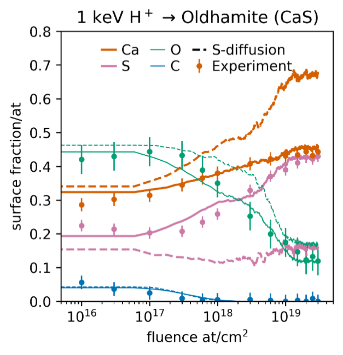
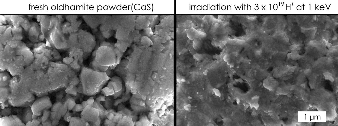
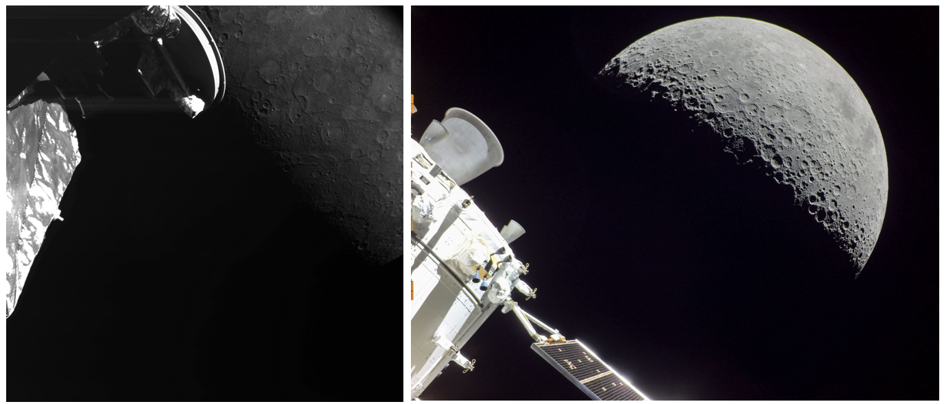
Figure 1. Left: Flyby image from the BepiColombo mission [10]. Right: Flyby image from the Artemis I mission [11].


Results
Figure 2 shows the color-coded SAfS DEM for the BepiColombo image. We found that the algorithm successfully reconstructed the surface in the center of the image but struggled with the more extremely illuminated sections at the edges. It is obvious that the algorithm reconstructed some details that are not visible in the input DEM and hence improved the resolution. Figure 3 compares a grey-scale representation of the SAfS DEM with MDIS WAC image EW0251718878F. Small craters in Izquierdo (the crater in the right half of the marked section), a few kilometers in diameter, become especially visible. Figure 4 shows the marked section in more detail. Due to the lack of high-resolution ground truth, a detailed algorithm evaluation was not possible for this image.

Figure 2. Color-coded presentation of the reconstructed SAfS DEM from the BepiColombo image.


Figure 3. Left: grey scale reconstructed SAfS DEM from the BepiColombo image. Right: wide-angle camera (WAC) image from MDIS [8]. The marked image section was evaluated in more detail (Fig. 4).


Figure 4. Comparison of WAC image, input DEM, BepiColombo (BC) image and SAfS DEM. Below the images are the height and slope of the profile (red dashed line).


However, the ground truth evaluation with the Artemis I image gives a quantitative measure under comparable conditions. Figure 5 shows the color-coded SAfS DEM of a region of interest (ROI) reconstructed from the flyby image. The results for the Artemis I image for all ROIs were of high quality. Figure 6 shows the elevation profile indicated by the dashed line in Figure 5. The algorithm refines the low-frequency initial DEM (dashed line), yielding a SAfS DEM (red line), which closely resembles the ground truth DEM (black line).  The vertical RMSE between the reconstructed DEM and the ground truth is 523 m, lower than the pixel size of approximately 1500 m. However, there were inaccuracies near the ROIs’ edges, and a preferred direction aligned with the illumination direction became visible.

Figure 5. Color-coded presentation of the reconstructed SAfS DEM from the Artemis image. The black dashed line marks the profile that was analyzed in detail (see Fig. 6).


Figure 6. Height profile of a selected terrain profile (see black dashed line in Fig. 5). Red line: DEM generated with the SAfS algorithm. Black line: Ground truth DEM. Dashed line: Initial DEM (input for the SAfS algorithm).


Conclusion
In conclusion, it is possible to obtain sharp results by applying our SAfS framework to flyby images. Both results show that, despite the challenging conditions, the SAfS algorithm could reconstruct the surface up to image resolution and increase the level of detail of the input DEM. The quality differences between the two images can mainly be attributed to the (spatial) resolution of the original images and the oblique illumination direction. Usually, the image center is distortion-free, and the illumination geometry is best suited for SAfS. We found that the surface reconstruction at the edge of the image is also possible, but the quality decreases significantly. All in all, our flyby-derived DEMs are accurate, and a previous version has been used for ESA outreach activities, similar to [12]:
https://www.esa.int/Science_Exploration/Space_Science/BepiColombo/BepiColombo_s_third_Mercury_flyby_the_movie


References
[1] A. Grumpe, F. Belkhir, C. Wöhler. Advances in Space Research, 53(12):1735–1767, 2014.
[2] C. Jiang, S. Douté, B. Luo, L. Zhang, P&RS,130, 2017 
[3] O. Alexandrov, R. Beyer. Earth and Space Science, 5, 2018
[4] B.  Wu, W. C.  Liu, A. Grumpe, C. Wöhler. P&RS, 140, 2018
[5] M. Tenthoff, K. Wohlfarth, C. Wöhler. Remote Sensing, 12(23), 2020.
[6] M. Hess, M. Tenthoff, K. Wohlfarth, and C. Wöhler. Journal of Imaging, 8(6), 2022.
[7] J. Warell, Icarus, 167, 2,2004
[8] Hawkins, S. Edward, et al. Space Science Reviews 131 (2007): 247-338.
[9] M.K. Barker, E. Mazarico, G.A. Neumann, M.T. Zuber, J. Haruyama, D.E. Smith, Icarus, 273, 2016.
[10] ESA. Planetary science archive.2023.
https://archives.esac.esa.int/psa/#!Image%20View/MCAM=instrument, accessed 10th May 2024
[11] NASA. flickr, 2022,
https://www.flickr.com/photos/nasa2explore/52547180935/in/album-72177720303788800/, accessed 10th May 2024
[12] K. Wohlfarth, M. Tenthoff, J. Wright, V. Galluzzi, C. Wöhler, H. Hiesinger, J. Helbert, J. Zender, J. Beckhoff. MExAG Annual Meeting, 02.2023

How to cite: Krüll, I., Wohlfarth, K., Tenthoff, M., Wöhler, C., Galluzzi, V., Wright, J., Benkhoff, J., and Zender, J.: Shape and Albedo from Shading with Planetary Flyby Images of Mercury and the Moon, Europlanet Science Congress 2024, Berlin, Germany, 8–13 Sep 2024, EPSC2024-247, https://doi.org/10.5194/epsc2024-247, 2024.

EPSC2024-851
|
On-site presentation
Cristina Re, Adriano Tullo, Riccardo La Grassa, Natalia Amanda Vergara, Gabriele Cremonese, and Emanuele Simioni

Introduction

The observation of planetary surfaces is often a complex task, where maximizing the science output and targeting unknown or poorly known features can require a certain amount of imaging data. Also, supporting the development of tools and methodologies for advanced imaging analysis requires data for testing and validation. Real datasets from previous missions are not always available or suitable for these aims and one way is to simulate datasets of imagery representing the operational scenarios as close to reality as possible.

A solution for the creation of synthetic images is to use physics-based rendering with Ray Tracing techniques.

This work is placed in the context of the remote sensing imaging sensors and it will take advantage of the case of the SIMBIO-SYS (Spectrometer and Imagers for MPO BepiColombo Integrated Observatory System) [1] instrument suite on board the BepiColombo mission for validation and testing. The work consists into developing a complete framework/tool for creation of simulated images for all three channels of SIMBIO-SYS.


The Simulator

The SIMBIO-SYS simulated image dataset has been created by arranging a planetary surface image simulator that includes Python scripts interfaced with the open-source software Blender taking advantage of its high-performance ray-tracing engine “Cycles” for the generation of photo-realistic and physics-based images.

The starting point is the AIS simulator [2] provided by the University of Helsinki. This software is directed, so far, to evaluate the performance of cameras devoted to the imaging of asteroids and comet nuclei. We had remodeled and enhanced this tool for our purposes that consider, as main targets, regions on extended planetary surfaces with a certain composition variability determined by spectrally different materials. The performances of the simulations imply that the variability of surface properties (local albedo or color, for example) is introduced by using Blender’s procedural modeling tools.

The AIS has been the base skeleton from which starting to develop a complete tool that, properly integrated with specific plugins and routines, could represent an important support to the scientific community. This tool will be critical/crucial during missions planning phase and in developing advanced tools to  fully and efficiently utilize the scientific data. The strengths will be the possibility to access the specific geometry of the acquisition and the actual trajectory and attitude of the spacecraft thanks to the SPICE kernel implementation [3]. Furthermore, the surface of the planet will be emulated by importing, in the virtual environment of the renderer, Digital Terrain Models (DTMs) of the observed surface, where available, or high-resolution planetary analogues. This approach will allow to perform the rendering of a surveyed region and to provide a virtual imaging completely coherent with reality. The target that occupies the scene is imported in Blender as a mesh composed of polygonal faces having various properties (called “materials”) that affect the reflection and/or emission of light in different ways. The system will consent to encode the spectral response of different simulated materials (from different geological composition) on the observed surfaces (Figure 1). The source of the spectra will be derived from real data or synthetically from spectral models. The source of the spectra will derive from real data or synthetically from spectral models. Furthermore, in Blender the intensity of the light source and the photometric properties of the objects can be defined allowing to derive the image data in actual physical units. A significant advantage of an open physically based renderer is the possibility of implementing more realistic and accurate photometric models (such as Hapke).


Figure 1: a) The mesh of a crater. b) Regions identified for each assigned material.

Application

As starting case study and validation testing for the framework, we considered to reproduce the future acquisitions of the three SIMBIO-SYS channels, the stereo images of STC (Example in Figure 2), the high-resolution images of HRIC and the hyperspectral cubes of the VIHI channel. The tool will be able to reproduce various realistic scenarios of the BepiColombo mission, creating highly accurate simulated datasets of panchromatic or multi/hyper- spectral acquisitions that will allow us to:

  • analyze implications in the planning of SIMBIO-SYS observations on specific targets based on detailed and reliable simulations, verifying how different spectral and spatial details can be resolved with the three channels.
  • provide a large, simulated dataset to support development and testing of tools for advance image processing and analysis such as the mosaicking methodologies.

One of the purposes of the developed tool is to support, with the simulated datasets, the planning of SIMBIO-SYS observations on scientific targets, such as the permanent shadowed regions (PSR), hollows, volcanic edifices, and tectonic structures. The analysis of this kind of reliable simulation datasets can provide indications on how different spectral and/or spatial details can be resolved with the SIMBIO-SYS channels. The tool can be very important to the science team involved in the definition of the target to obtain a realistic impression of the future acquisition and drive the temporal planning of such specific features. Disposing of simulated images will provide a direct evaluation of the optimal conditions to satisfy and to constrain during the planning. The tool will open the possibility to perform investigations about the influence of the illumination conditions on the target acquisitions providing invaluable support to planning activities.

Figure 2: On the top, graphical visualization of the spectral ranges of the STC filters. At the bottom, example of simulated STC acquisitions for both the sub-channels.

References

[1] Cremonese, Gabriele, et al. SIMBIO-SYS: scientific cameras and spectrometer for the BepiColombo mission. Space science reviews, 2020, 216: 1-78.

[2] Penttilä, Antti, et al. Blender modeling and simulation testbed for solar system object imaging and camera performance. No. EPSC2022-788. Copernicus Meetings, 2022.

[3] Acton, Charles H. Nasa’s spice system models the solar system. In: International Astronomical Union Colloquium. Cambridge University Press, 1997. p. 257-262.


How to cite: Re, C., Tullo, A., La Grassa, R., Vergara, N. A., Cremonese, G., and Simioni, E.: PLanetary Image Simulator (PLAS) tool and applications for MPO SIMBIO-SYS camera simulations, Europlanet Science Congress 2024, Berlin, Germany, 8–13 Sep 2024, EPSC2024-851, https://doi.org/10.5194/epsc2024-851, 2024.

EPSC2024-333
|
ECP
|
Virtual presentation
Vesa Björn, Karri Muinonen, Antti Penttilä, and Deborah Domingue

Mercury can be modeled as an atmosphereless Solar System body. Such objects are covered by a regolith which affects how they scatter light. To deduce physical properties of Mercury’s regolith, we use spectrophotometry from the MDIS (Mercury Dual Imaging System) instrument of NASA’s MESSENGER (MErcury Surface, Space ENvironment, GEochemistry and Ranging) mission. The data comes in eight colors [1] between the wavelengths of 433.2 nm and 996.2 nm, with phase angles from 20 to 130 degrees. There are 37752 data points, of which we use 26610 that are at incidence and emergence angles below 70 degrees. 
A theoretical particulate-medium model is used to interpret the observed reflectance. The model includes a shadowing correction that depends on three geometry parameters of the regolith. The first parameter is the packing density ν, i.e., the ratio of the particles’ volume to the total volume. The other two parameters describe the regolith’s roughness as a fractional Brownian motion (fBm) surface: the Hurst exponent H in the horizontal and the amplitude σ in the vertical direction. 
The numerical implementation of the model includes a set of discrete parameter values [2]. However, using trilinear interpolation, we extend the parameters to have arbitrary values within the range of the discrete values, which are 0.15–0.55 for the packing density, 0.20–0.80 for the Hurst exponent, and 0.00–0.10 for the amplitude (in units of the width of the simulated medium). We optimize the model parameters in least-squares sense using the Nelder–Mead simplex method, followed by Markov chain Monte Carlo (MCMC) sampling that uses proposed parameter values drawn from Gaussian distributions. The model parameters are solved for all wavelengths simultaneously, which means that the result is physically consistent. In the present study, the size of the regolith particles follows a uniform distribution between 0.0006 and 0.003, in units of the medium width. 
Our results indicate that Mercury’s regolith is densely packed (ν = 0.541 ± 0.010) with moderate horizontal variations (H = 0.529 ± 0.009) and large height variations (σ = 0.098 ± 0.002). The MCMC solution allows us to predict the spectrophotometry for differing viewing geometries. Future work includes updating the implementation of the model by increasing the range of the parameter values, especially for the packing density to ν > 0.55. Another improvement is to modify the size distribution of the regolith particles. The results of our study can be utilized in the BepiColombo mission, which will start its science mission in early 2026.  

[1] Domingue et al., Icarus 257, 477 (2015)
[2] Wilkman et al., Planet. Space Sci. 118, 250 (2015)
[3] Nelder and Mead, Comput. J. 7(4), 308 (1965)

How to cite: Björn, V., Muinonen, K., Penttilä, A., and Domingue, D.: Spectrophotometric modeling of Mercury’s regolith using MESSENGER MDIS data, Europlanet Science Congress 2024, Berlin, Germany, 8–13 Sep 2024, EPSC2024-333, https://doi.org/10.5194/epsc2024-333, 2024.

EPSC2024-215
|
On-site presentation
Andreas Morlok, Iris Weber, Maximilian P. Reitze, Aleksandra N. Stojic, Stephan Klemme, Jan H. Pasckert, Karin E. Bauch, Harald Hiesinger, and Jörn Helbert

Introduction: The MERTIS (MErcury Radiometer and Thermal Infrared Spectrometer) onboard of the BepiColombo ESA/JAXA mission to Mercury is a mid-infrared instrument that will allow mapping the hermean surface from 7 µm to 14 µm [1,2]. After arrival in 2025, a database for the interpretation of the data is needed. As part of this effort, we have studied rock samples like impact rocks and meteorites [e.g,. 3]. A second field of interest are analogs synthesized based on data by MESSENGER [e.g., 4].

Based on recent modeling of the oxidation state of the hermean surface, a highly reducing environment can be expected [5,6]. Likewise past volcanism or impact experiments suggest the presence of extremely reduced phases, e.g., Si-metal (e.g, 7, 8]). This implies that in addition to common minerals (pyroxene, plagioclase), also oxides (corundum, spinel, periclase), metallic phases, halides, and reduced variations e.g. of olivine (Ca-olivine Larnite) are possible. As part of our database project, we cover this type mineral phases.

Samples and Techniques: We characterized the materials first with EMPA. Samples were ground and sieved into grain four size fractions (<25 µm, 25µm-63 µm, 63µm-125 µm and 125µm-250 µm). Mid-infrared reflectance spectra were obtained from 2-18 µm with a Vertex70v at the IRIS lab at the Institut for Planetologie, University of Münster. Always 512 scans were averaged, a diffuse gold standard was applied for calibration.    

Results: A strong Reststrahlenband (RB) between 12.2 µm and 12.5 µm is typical for SiC. The Christiansen Feature (CF), a characteristic low-point, is at 10.1 µm.

No features are seen in metallic Si. The spectrum is a continuum in the mid-infrared that increases towards longer wavelengths.

The spectra for oxides are fundamentally different: They exhibit a trough-like low in the very range where silicates have their characteristic RBs. For ilmenite, the low is from 11.7 µm to 11.9 µm, for rutile from 11.1 µm to 11.3 µm and corundum shows a broad low at from 8.4 µm -10.0 µm. These low-points are also the CF. In addition, corundum exhibits absorption-like bands from 12.4 µm to 15.9 µm.

Summary & Conclusions: There are clear differences between silicates and oxides: The broad low from 8.4 µm – 11.4 µm is where silicates have their RBs. This would give even low abundances of oxides a big influence on the general spectral shape. Refractory SiC has a spectrum similar to silicates, the CF at 10.1 µm is at clearly longer wavelength compared to silicates. Similar, the broad ‘low’ of the oxides would shift the CF to longer wavelengths.    

References: [1] Hiesinger et al. (2020) Space Sci Rev. 216, 8, id.147. [2] Benkhoff, J. et al. (2021) Space Sci Rev. 217, 8, id.90. [3] Morlok et al. (2016) Icarus 264, 352-368 [4] Morlok et al. (2021) Icarus 361, [5] McCubbin et al. (2017) JGR Planets 122, 2053-2076 [6] vander Kaaden et al. (2017) Icarus 285, 155-168  [7] Stojic et al. (2022) EPSC 2022, Abstract No. EPSC2022-813. [8] Iacovino et al. (2023). Earth and Planetary Science Letters, 602, 117908.


Fig.1: (Left) Reflectance mid-infrared spectra for SiC (Top) and metallic Si (Bottom). The metallic Si shows features in the MERTIS range (dotted area, 7-14 µm). SiC on the other hand exhibits a RB from 12.2 µm to 12.5 µm. (Right) Oxides show a similar shape, a trough-like low in the MERTIS range. The CF for oxides is shifted compared to silicates.

Hatched area: characteristic bands for typical silicates enstatite (En) and forsterite (For), which tend to form in the low area of the oxides. Shaded area: range of the MERTIS instrument.

How to cite: Morlok, A., Weber, I., Reitze, M. P., Stojic, A. N., Klemme, S., Pasckert, J. H., Bauch, K. E., Hiesinger, H., and Helbert, J.: Oxides and Reduced Phases in the Mid-IR: Data for the BepiColombo Mission to Mercury , Europlanet Science Congress 2024, Berlin, Germany, 8–13 Sep 2024, EPSC2024-215, https://doi.org/10.5194/epsc2024-215, 2024.

EPSC2024-337
|
ECP
|
On-site presentation
Pamela Cambianica, Emanuele Simioni, Gabriele Cremonese, Silvia Bertoli, Elena Martellato, Alice Lucchetti, Maurizio Pajola, Cristina Re, Adriano Tullo, and Matteo Massironi

Introduction: Earth-based radar observations revealed areas within Mercury’s north polar regions with peculiar high radar backscatter [1,2]. The presence of this radar-bright material was interpreted as water ice within permanently shadowed regions (PSRs) because the radar characteristics resemble those observed for the Martian polar ice caps. [3] indicated that Mercury’s polar environment is capable of hosting stable water-ice-deposits over geologic time-scales. Later, the MErcury Surface, Space ENvironment, GEochemistry, and Ranging (MESSENGER) mission has suggested that these radar-bright materials are predominantly composed of water ice. The detection, global mapping, and analysis of the composition of PSRs with an unprecedented high-resolution are among the primary scientific goals of the Spectrometer and IMagers for MPO Bepicolombo Integrated Observatory SYstem (SIMBIO-SYS) suite [4].

Understanding these features can provide key insight into the evolution and composition of Mercury’s volatile polar deposits. However, interpretation of the highest-resolution images of Mercury’s polar deposits is limited by the availability of illumination and thermal models. In fact, estimation of illumination conditions and calculation of the surface radiative intensity on the surface of Mercury are fundamental to study the effect of the insolation weathering affecting the PSRs. These areas can receive only scattered light, emitted thermal energy from the surrounding topography, and thermal energy from Mercury's interior. To obtain the surface and subsurface temperature distributions of an airless body, any thermophysical model than aims to consider realistic physical conditions such as topography, orbital elements, surface roughness, and thermophysical parameters (e.g., thermal inertia or thermal conductivity) needs to consider two illumination cases occurring on a surface: 1) the direct and 2) the scattered sunlight cases. In the case of Mercury, the solar disk cannot be approximated as a point source, and the back scattered light needs to be considered. This allows to quantify the self-heating effect, which results from the absorption of thermal radiation by elements of the topography from surrounding visible portions. As a result, the coldest facets can be heated by the hotter ones, increasing the total amount of insolation received by the surface.

In this work we aim to quantify the thermal impact of incorporating scattering and self-heating effects into simulations of temperature distribution on airless surfaces. Our focus is on the Laxness (83.27°N  50.04°W, diameter 27 km) and Fuller (82.63°N, 42.65°W, diameter 25.9 km), craters, situated in the northern regions of the Goethe Basin.

These craters, with their unique shapes, depths, and rim heights, offer valuable insights into the interplay between sunlight scattering, shadowing effects, and thermal behavior in extreme conditions. By examining these craters, we aim to enhance our understanding of the thermal processes at play in Mercury’s polar regions, contributing to a more comprehensive model of planetary surface temperatures.

Method: To investigate the role of the self-heating effect on the PSRs we developed a ray-tracing illumination and 3D Eulerian thermal model. Calculations were performed by using local Digital Terrain Models (DTMs), generated by [5], of Mercury’s north polar craters with a resolution of 125 m/px. The crater DTM was used as input of the solar illumination model. The model is based on the ray-tracing technique and treated the Sun as a disk and not as a point source due to the proximity of Mercury to the Sun. This illumination model allows to trace solar rays to each point on the DTM evaluating the direct illumination throughout a Mercury solar day. Meshes are then input into the 3D thermal model and the model is given an initial temperature based on latitude. The thermal model computes the surface temperature of each facet of the geometry as it evolves over time. The temperature is calculated by balancing direct insolation, multiple scattering of visible and infrared radiation from other facets, infrared emission, and 1D subsurface heat conduction. The effect of terrain shadowing is included.

Results: Figure 1 shows an example of how scattering affects the dispersion of energy received by the crater’s surface is illustrated. On the left, the direct radiation in W/m2 at a specific epoch can be observed, having simulated a period of 176 Earth-days. On the right, the areas of the crater where radiation is scattered (indicated as a percentage) are highlighted. There are regions that are impacted by solar flux through indirect insolation, due to the craters’ morphology. In order to understand how scattering affects the crater’s temperature, particularly in the PSRs, we calculated the temperature variation over the same time range. An example of maximum temperature profiles for the Fuller craters are presented in Fig. 2. For those plots, we developed an ad hoc method that allows us to extract a temperature profile from a heat map at a specific epoch, enabling the analysis of temperature variations for each pixel. This approach allows us to quantify even the smallest temperature changes. Additionally, in Fig. 3 the area where PSRs occur is indicated to enable accurate selection of the profile and facilitate the comparison with areas affected by direct radiation. There is a noticeable increase in temperature greater than what is observed in areas that receive direct illumination. To better quantify this effect, we averaged the maximum temperature variation between the two scenarios and calculated the percentage variation over the 176 Earth-days. For Laxness we found that the data cluster around the 15% average variation. On the contrary, the Fuller crater exhibits values around the 10% average variation. Each measure corresponds to a single day’s maximum temperature variation within the PSRs.


Acknowledgments: we gratefully acknowledge funding from the Italian Space Agency (ASI) under ASI-INAF agreement 2017-47-H.0

References: [1] Slade, M. A., Butler, B. J., & Muhleman, D. O. (1992).  Science258(5082), 635-640. [2] Butler, B. J., Muhleman, D. O., & Slade, M. A. (1993). Journal of Geophysical Research: Planets98(E8), 15003-15023. [3] Paige, D. A., Wood, S. E., & Vasavada, A. R. (1992). Science258(5082), 643-646. [4] Cremonese, et al. 2020, Space science reviews, 216, 1. [5] Hamill, et al. 2020, The Planetary Space Science journal 1.3:57. [6] Deutsch, et al., 2016a, Icarus 305, 139-148.


How to cite: Cambianica, P., Simioni, E., Cremonese, G., Bertoli, S., Martellato, E., Lucchetti, A., Pajola, M., Re, C., Tullo, A., and Massironi, M.: The thermal impact of the self-heating effect on airless bodies. The case of Mercury’s north polar craters. , Europlanet Science Congress 2024, Berlin, Germany, 8–13 Sep 2024, EPSC2024-337, https://doi.org/10.5194/epsc2024-337, 2024.

EPSC2024-840
|
ECP
|
On-site presentation
Silvia Bertoli, Pamela Cambianica, Elena Martellato, Gabriele Cremonese, Alice Lucchetti, Maurizio Pajola, Giovanni Munaretto, Matteo Massironi, and Emanuele Simioni

Introduction: The polar regions of Mercury host Permanent Shadowed Regions (PSRs), which are constantly in shadow (due to the planet’s small obliquity, [1]), and can thus reach very low temperatures [2]. These conditions might have facilitated the long-term survival of water ice, as suggested in the 90s after the discovery of radar bright material within the PSRs by Earth-based observations [3]. This hypothesis was later confirmed through the comparison with the signal from icy satellites and Mars’s polar cap [4], hydrogen concentration on PSR measured from MESSENGER mission [5], and thermal models [6]. The morphological analysis of such craters in [7] highlights some interesting features within them that may be attributed to water ice. In this work, we show the results obtained by applying a shape-based thermophysical model [8] to 1) characterize the thermal environment; 2) predict the evolution of the analysed craters [7]; and 3) understand if the PSRs thermal conditions could affect the occurrence and evolution of specific landforms.

Method: Two different methodologies are used to explore the thermal behaviour of craters located in the north pole of Mercury. We start our evaluation from [7], focusing in specifying morphologies within Fuller crater (82.63°N, 42.65°W, diameter 25.9 km) and their potential thermal implications. Secondly, we performed a thermal analysis in order to evaluate the possible implication of the temperature on these morphologies. To investigate the thermal environment of the analyzed craters we applied a shape-based thermophysical model [8]. It employs ray tracing techniques and treats the Sun as a disk, reflecting the proximity of Mercury to the Sun and the resulting extensive coverage of the Sun in Mercury’s sky. By considering the Sun as a disk, this makes shadow and penumbra modeling more thorough and complete in terms of heat flux calculation. Indeed, the actual morphology of a crater strongly affects the final amount of insolation received from a geometry element.

Morphological analysis: The first type of morphologies concerns the fractures present in the PSRs within Fuller crater. These have been classified as “Landforms of Uncertain origin” by [7] because their morphogenesis cannot be unambiguously defined at the available resolution. One hypothesis explaining the formation of these landforms is that the subsurface ice could act as permafrost. For instance, on Earth, permafrost forms when ground is frozen for more than two years [9]. Previous studies (e.g., [6,11]) highlighted that craters with PSRs have a characteristic lag deposit on their floor, defined as dark carbon rich-material, representing the leftover of sublimated ice. This layer could act as a permafrost active layer, which flows and produces cracks on the surface, when assuming that the freeze cycle in penumbra areas is affected by heat transfer from the nearby permanently illuminated area [12]. Alternatively, we cannot exclude the possibility that fractures could instead form from the cooling of impact melt material and/or volcanic infilling. In fact, many of those kinds of fractures have been observed on Mercury [13].

A second characteristic feature is landslides, which can partially cover crater’s floor. Its peculiarity relies on being formed after crater formation and is referred as “rockslide [14]. Its occurrence can be explained by the thermal weathering rate, which may result in varying volumes of regolith that are subject to failure. The effectiveness of weathering may be reduced in the areas of the Hermean polar craters that are permanently shaded, causing the decrease of the probability of later landslides.

The third feature is the “Rough unit” [7] presents in the Fuller floor, placed just next to the central peak, rough and with a dark grey tone. It appears completely different from the smooth floor and the landslide material, thus it become really intriguing to investigate its origin.

Preliminary observations: The plot in Fig. 1 shows the max temperatures measured in 173 days, reached by different portion of the crater (the colored curves are the different profiles). From the graph, it is possible to notice:

  • The part of the floor with fractures experiences a maximum temperature T of 200 K;
  • The blue unit (Rough unit) reached the lowest T (around 150 K). This is intriguing because it corresponds to the area where the presence of radar-bright material has been observed. Therefore, it could represent a morphology very similar to terrestrial debris-covered glaciers;
  • The surface affected by landslide undergoes significant temperature fluctuations, ranging from 300 K to 550 K within a distance of less than 10 km.

Conclusions and future works: We focused our attention on craters with PSRs in the north pole of Mercury. In particular, based on [7], we selected specific morphologies (e.g. fractures, landslides), whose origin and evolution could be connected to the specific temperature conditions of the hermean poles. The next step involves applying the thermal model by [8] to these specific structures, in order to assess the potential influence of thermal conditions on the evolution of those craters and the ice deposits within them.

Acknowledgements: The study has been supported by the Italian Space Agency (ASI-INAF agreement no. 2020-17-HH.0).

References: [1] Margot J.-L. et al. (2012), JGR: Planets, V. 117. [2] Susorney H. C. M. et al. (2021), The Planet. Sci. J., V. 2., p. 97 [3] Harmon and Slade (1992), Science, V. 258(5082), pp. 640– 643 . [4] Butler et al. (1993), JGR, V. 98, pp. 15003 – 15023. [5] Wilson et al. (2019), JGR:Planets, V. 124, pp. 721 – 733. [6] Paige et al. (2013), Science, V. 339, pp. 300 – 303. [7] Bertoli et al. (2024), Journal of Maps, accepted [8] Cambianica P. et al (2024), PSS, Subm. [9] Dobinski, W. (2011), Earth-Science Rev., V. 108, pp. 158 – 169. [10] Syal M. B. et al. (2015), Nature Geoscience, V. 8., pp. 352 – 356. [11] Filacchione G. et al. (2022), EPSC Abstracts V. 16, EPSC2022- 191, 2022 [12] Xiao Z. et al. (2014b), JGR:Planets, V. 119, pp. 1496 – 1515. [13] Crudes D. M. and Varnes D. J. (1996), Landslides Eng. Pract, V. 24, pp. 20–47. [14] Brunetti M. T. et al. (2015), Icarus, V. 260, pp. 289 – 300.


How to cite: Bertoli, S., Cambianica, P., Martellato, E., Cremonese, G., Lucchetti, A., Pajola, M., Munaretto, G., Massironi, M., and Simioni, E.: Interplay between morphology and thermal conditions within the Permanent Shadowed Regions, North pole of Mercury., Europlanet Science Congress 2024, Berlin, Germany, 8–13 Sep 2024, EPSC2024-840, https://doi.org/10.5194/epsc2024-840, 2024.

EPSC2024-450
|
ECP
|
On-site presentation
Barbara De Toffoli, Valentina Galluzzi, Matteo Massironi, Sebastien Besse, Gene Walter Schmidt, Oceane Barraud, Salvatore Buoninfante, and Pasquale Palumbo

Introduction

Mercury's hollows are small (tens of meters to few kilometers), localized, shallow depressions found on the surface of the planet. They are unique features distinct from their surroundings, and characterized by their appearance as irregular, bright spots, often found clustered in groups called hollow fields. Their origin is still not fully understood, but they are believed to be related to sublimation processes, where volatile materials [1; 2] close to the surface directly transition from solid to gas due to exposure to high temperatures due for example to intense sunlight or volcanic activity [3]. However, as the ESA/JAXA BepiColombo spacecraft is approaching Mercury [4], understanding the specific geological and environmental factors influencing the formation and distribution of hollows remains a key research objective [5]. 


Methods

To improve our grasp on this topic, we herein renew the previous hollows dataset provided by [7] by updating the database and its degree of detail. Indeed, in this work we make use of MESSENGER end of mission mosaic datasets [6] in order to exploit the most updated data that were not yet available at the time when the previous database [7] was released. We provide GIS-ready polygonal features to encompass areas where fields of hollows are present on the surface and present a statistical analysis on their occurrence across the surface. We also provide statistical information on the craters hosting hollows and compare them to the global crater database [8]. This study aims at understanding the global stratigraphic occurrence of hollows through a statistical approach, setting a foundation for future multidisciplinary research, rather than focusing solely on their intrinsic morphology or composition. By compiling this updated global database of hollows, we can preliminarily explore their stratigraphic occurrence to investigate their debated formation origins. Since most of the population of hollows is contained within impact craters, which by definition excavate the crust of the planet exposing the underlying stratigraphy, it is possible to investigate whether relationships exist between the presence of hollows and specific crater populations and, in turn, constrain whether there is one or more identifiable source layers. Specifically, to profitably test these hypotheses, we compared the population of craters containing hollows (c. 430 in total) and an existing dataset of craters on Mercury [8]. This database, that we will refer to as the global population, is based on a thorough mapping effort that provided a broad and nearly global coverage of Mercury craters by classifying them into 5 morphological classes [8]. Although other datasets exist, and this one includes only craters with diameters larger than 40 km, it represents one of the most recent and complete datasets available that also considers morphological classification for a statistically significant number of craters. By comparing diameter, depth, and degradation between the two crater datasets, it is possible to reveal differences between the global crater population and the subpopulation of hollow containing craters. This helps understanding whether the hollow containing craters are a random subset of the global population, and thus closely replicates its main characteristics (i.e. diameter, elevation, degradation), or not.


Results

Hollows occurrence seems to be ubiquitous and variously spatially correlated with multiple surface morphologies, foremost among them impact craters. In conclusion, the nuanced relationship between hollows and Mercury's geological history unveils the intricate interplay of endogenous and exogenous processes. The dynamic nature of hollows, with their occurrence in association with both impact and volcano-tectonic events, hints at a complex history of material redistribution on the planet's surface. Overall, we provide quantitative evidence supporting: 1- the lack of a single (or a limited and measurable number) planet-wide unit bearing the volatile materials necessary for hollows formation due to: (i) widespread depth range of hollows appearance in the crust; (ii) lack of correlation between hollow emergence and one or more geological units (including color units). 2- the short-lived nature of hollows due to: (i) a significant lack, or total absence, of hollows in older and more degraded craters compared to younger, fresher craters; (ii) a higher abundance of hollows correlated to tectonic structures or pits when located within older and degraded craters. Hence, from a stratigraphic point of view, this work highlights the likely existence of widespread presence of a both horizontally and vertically discontinuous volatile-bearing formation.


References

[1] Blewett, D., et al. (2013). JGR-Planets, 118, 1013–1032. [2] Barraud, O., et al., (2020). JGR-Planets, 125, e2020JE006497. [3] Blewett, D., et al. (2011). JGR-Planets, 116(E12). [4] Benkhoff, J., et al., (2021). Space Sci Rev, 217(8), 90. [5] Rothery, D., et al., (2020). Space Sci Rev, 216, 1-46. [6] Denevi, B.W., et al., (2018). Space Sci. Rev. 214, 2. [7] Thomas, R. J., et al., (2014), Icarus, 229, 221–235. [8] Kinczyk, M. J., et al., (2020). Icarus, 341, 113637.


Acknowledgement

Authors from Italian Institutes acknowledge Italian Space Agency (ASI) support within SIMBIOS-SYS project under ASI-INAF agreement 2017-47-H.0. Some of the authors gratefully thank the European Union – NextGenerationEU and the 2023 STARS Grants@Unipd programme – “HECATE project” support.

How to cite: De Toffoli, B., Galluzzi, V., Massironi, M., Besse, S., Schmidt, G. W., Barraud, O., Buoninfante, S., and Palumbo, P.: Hollows on Mercury: A Comprehensive Analysis of Spatial Patterns and Their Relationship to Craters and Structures, Europlanet Science Congress 2024, Berlin, Germany, 8–13 Sep 2024, EPSC2024-450, https://doi.org/10.5194/epsc2024-450, 2024.

EPSC2024-576
|
On-site presentation
Cristian Carli, Francesca Zambon, Lorenza Giacomini, Barbara De Toffoli, Anna Galiano, Matteo Massironi, Valentina Galluzzi, Fabrizio Capaccioni, and Pasquale Palumbo

Introduction

Hollows are one of the peculiar surface features that was highlighted by the MESSENGER mission [e.g. 1]. They have morphological evidence showing flat-floored and rimless depressions often clustered in fields and relatively bright. They are also associated with a peculiar cyan color within the RGB of the enhanced color mosaic [2]. This color variation is mainly indicating a higher reflectance, in particular within the visible, and a consequent bluer slope within the 400-1000 nm wavelength range [3]. In a few cases, such as the hollow field in the Dominici crater, literature has reported a potential absorption band in that spectral range [e.g. 4,5] with an inflection around 1000 nm, which could indicate an absorption [5]. The putative absorption has been attributed to some sulfides (e.g. CaS, [4]) or to the presence of transitional elements, different from iron, on silicates [5]. Here we investigate different hollow fields and other bright features with hollow-like (i.e. Dominici-like) spectral properties, present in the Kuiper quadrangle.

Data and Analytical Approach

MDIS 8 color mosaics have been produced with the same process described in [6] at different spatial resolutions taking care of the original image resolution, avoiding those frames with extreme geometrical values and pixel resolution larger than 3.6 km (see also [7]). We investigate the spectral properties of the hollow fields mapped by [8], as well as other bright features with cyan colors in the enhanced color mosaics.

Results

The spectral properties of the investigated features show in general a bluer slope and higher reflectance with respect to those of the Hermean average spectrum (see fig.1). Interestingly, the brighter features show the same spectral properties of Dominici hollow field present on the central peak: a potential absorption around 630-750 nm and an inflation towards 1000 nm. Hollow fields with these properties (first group) are, for instance, in Homer, Warhol, and Abu Navas craters. A second set of features show similar spectral properties with a slightly lower reflectance, and weaker, but still recognizable, absorption and inflation. This behavior is present for example in hollow fields of Chaickowski, Yets, Veronese craters, as well as some small bright features (probably small craters) like those closer to Yets and Beck craters. A third group with reflectance variable between the previous two groups shows the same spectral shapes but the absorption around the 630-750 nm is absent whereas the inflation towards the longer wavelengths is still present. In this case we have, for example, the second hollow field in Dominici and Abu Navas craters, with other small craters within the quadrangle. Further cases, in general those with a lower reflectance, show an intermediate slope, no absorption band, and a reduced, in some cases absent, inflection.

Discussion

All morphologically recognizable hollow fields present in the Kuiper quadrangle, maintain the same peculiar spectral properties reported in literature [4,5]. Spectra are dominated by a bluer spectral slope, they are relatively high in reflectance, but they can span from very bright up to an intermediate reflectance. Some of them clearly show an absorption like the one observed in the hollow field on the central peak of Dominici (first group); others show weaker absorption or inflection, up to spectra with a less blue slope and absence of the band and inflection. In general, those spectral properties peculiar to the hollow fields decrease with the reflectance of those regions. Where spectral properties of hollows become less evident, we find features like hollows but also like bright spots and small, fresh craters.

Hollow-like spectral properties seem to suggest that they are compositionally different from the surrounding and several cases, non-only in Dominici crater, since to have the same spectral evidence. Nevertheless, a transition between the materials present in the hollow fields and the cases where spectral properties become closer to the average spectrum of a hermean terrain seems to be present. Interestingly, this hollows-like material seems to be present in regions where we cannot clearly identify the presence of hollow fields by means of photo-interpretation yet.

 Implications

The variation of spectra within the different cases could be probably related to 1) a possible variation of the composition of the hollows, 2) mixing of the hollow-like constituent with different material from the surrounding terrains, 3) a different number density of hollows within the hollow fields, or 4) an increasing effect of space weathering (i.e. aging) or physical degradation of the hollow fields.

Moreover, there is evidence that similar spectral properties are present both in regions where hollow fields can be clearly identified, and in other small bright regions, often clearly associated with craters, where hollows have not been identified yet. This could indicate that the image resolution does not permit identifying hollow fields in those areas. Conversely, the similitude of spectral properties between hollow fields and other features could indicate the composition of a material forming part of the crust of Mercury, only exposed on relatively fresher regions.

Our future activity will focus on understanding better if the hollows-like material can be present not only in hollow fields and why we see a variation in its spectral properties. Moreover, we will suggest which of those could be the most interesting targets for the BepiColombo mission.

Acknowledgment

This research is funded from the Italian Space Agency (ASI) within SIMBIOS-SYS project under ASI-INAF agreement 2017-47-H.0. CC, FZ, GL, MM, VG were also supported by Europlanet RI20-24 research grant agreement No. 871149-GMAP.

References

[1] Blewett et al. (2011) Science 333. [2] Denevi et al. (2011) Science 333.  [3] Blewett et al. (2013) JGR 118. [4] Vilas et al. (2016) GRL 43.[5] Lucchetti et al. (2018) JGR 123. [6] Zambon et al. (2022) JGR 127. [7] Carli et al. 2022, CNSP XVII, Abstract#. [8] Giacomini et al. 2023, Journal of Maps 18.

How to cite: Carli, C., Zambon, F., Giacomini, L., De Toffoli, B., Galiano, A., Massironi, M., Galluzzi, V., Capaccioni, F., and Palumbo, P.: Hollows-like materials, what are their spectral properties telling us?, Europlanet Science Congress 2024, Berlin, Germany, 8–13 Sep 2024, EPSC2024-576, https://doi.org/10.5194/epsc2024-576, 2024.

EPSC2024-646
|
ECP
|
On-site presentation
Mireia Leon Dasi, Sebastien Besse, Lauren M. Jozwiak, Erica R. Jawin, and Alain Doressoundiram

Explosive volcanic activity on Mercury extended after the end of the widespread effusive volcanism era (Jozwiak et al., 2018). Understanding the precise timing of explosive eruptions has significant implications for the volatile content and thermal evolution of the planet. However, the age of individual pyroclastic deposits remains largely debated and is difficult to assess using crater counting (e.g. Luchitta and Schmitt, 1974). An individual analysis of a selection of faculae has highlighted the spectral diversity across and within deposits (Barraud et al., 2021, Besse et al., 2020). In this work, we constrain the link between the variability in spectral properties across deposits and deposit age. Additionally, we explore the spatial variability in spectral properties inside deposits, and the relationship of this variability to the timing of eruptions inside individual faculae. A combination of morphologic analyses based on MESSENGER/MDIS images and spectral data from MESSENGER/MASCS is analyzed to this end, utilizing a deep learning approach.

We analyze the relationship between the morphological degradation of the vents (physical depressions) and the spectral changes in the associated deposits (faculae). This study shows a correlation between the deposit spectra and vent degradation, characterized by a rapid initial darkening of the deposit and spectral flattening over time, followed by stabilization. The deposits with heavily degraded vents reach the properties of the local background terrain, rendering old deposits spectrally undetectable. To explain these temporal variations in spectral properties, we propose three potential processes: space weathering, mixing with the underlying terrain, and changes in erupted pyroclast size. Space weathering acts “fast”: spectral changes induced by nanophase iron accumulation produced by space weathering on the Moon saturate after ~1 Ga (Tai Udovicic et al., 2021). If a similar mechanism is responsible for most of the spectral modifications observed over time, then a large part of explosive eruptions detected on Mercury could be significantly younger than previously expected.

To explore the relative timing of vents within the same facula, we examine the variability of spectral properties inside the deposits. Using outlines defining the vent profile and the deposit extent defined by Leon-Dasi et al. (2023), we extract the evolution of spectral properties in the direction locally perpendicular to the vent. Using these data, we study (1) the rate of change of spectral properties, (2) the symmetry of the deposit, and (3) the contribution of each vent to the spectral variability. This analysis benefits from leveraging the deep learning-based data reduction performed by Leon-Dasi et al. (2023), which results in a set of latent dimensions integrating spatial and spectral information. Using such latent dimension has proven to highlight the pyroclastic deposits and reduce the spatial noise more effectively than using single MASCS-derived spectral parameters. From a preliminary analysis, we find a trend between the rate of change of the spectral variations across the deposits and the deposit age. Older deposits appear to present slower-changing spectral properties, which is consistent with deposit erasure over time through various space weathering processes. Within multi-vent faculae, we find spatial variations in the association between spectral signatures and different vents—this implies that eruptions within a single facula were separated in time. Overall, this research provides further insight into Mercury’s volcanic history and the processes that have shaped its surface over time.

How to cite: Leon Dasi, M., Besse, S., Jozwiak, L. M., Jawin, E. R., and Doressoundiram, A.: Spectral properties of pyroclastic deposits on Mercury over space and time, Europlanet Science Congress 2024, Berlin, Germany, 8–13 Sep 2024, EPSC2024-646, https://doi.org/10.5194/epsc2024-646, 2024.

EPSC2024-764
|
On-site presentation
Thomas Müller, Jon Fulbright, Gaku Nishiyama, Martin Burgdorf, and Shinsuke Uno

Thermal infrared (IR) observations of Mercury are scarce. Space observatories usually cannot measure so close to the Sun, twilight observations from ground are difficult, and the zodiacal background is very strong. Hansen (1974) determined Mercury's surface temperature and emissivity via IR photometer measurements at 3.8 and 4.7µm. Sprague et al. (1994) conducted spectroscopic observations (7.3-13.5 µm) of three locations on the surface of Mercury via an IR spectrometer at the InfraRed Telescope Facility (IRTF). They found evidence for Anorthosite and Basalt on the surface. Emery et al. (1998) interpreted two epoch mid-infrared (5-12 µm) measurements obtained from the Kuiper Airborne observatory via the High-efficiency Infrared Faint Object Grating Spectrometer (HIFOGS). They developed a new rough-surface thermal model for Mercury and looked into grain-size and surface composition aspects. Sprague et al. (2000a) presented a low-resolution N-band spectrum (8.1-13.25 µm) taken with Mid-Infrared Array Camera (MIRAC) at the Steward Observatory. The measurements were centered on a surface region which was not imaged by Mariner 10. The spectra included signatures of the surface roughness and mineralogy. Overall, the very few published datasets cover only a limited phase angle and wavelength range. And, many questions about Mercury’s thermal behaviour remain unanswered.

Recent works by Nishiyama et al. (2022) and by Fulbright et al. (2023) opened a new door to thermal observations of Mercury. Several geostationary weather satellites carry well-calibrated multi-band IR instruments and they detect Mercury very frequently when its apparent position is close to the Earth’s rim: Himawari-8/-9 (AHI instrument), GOES-16/-17/-18 (ABI instrument), and MeteoSat-8/-9/-10/-11 (SEVIRI instrument). They have 10 (AHI, ABI) or 8 (SEVIRI) well calibrated IR channels in the range between 3.9 and 13.4 µm. The measurements cover a phase angle range from about -160 to +160, including data at phase angles below 5(close to superior conjunction). The apparent size of Mercury varies between about 4.5 and 13 arcsec in diameter.

We interpret these measurements with a thermophysical model (TPM) of Mercury which is based on a lunar model (Müller et al. 2021), and uses published physical and thermal properties of Mercury’s surface. It explains the data obtained by the geostationary satellites very well and it can also reproduce the published IR spectra on a 5-10% level.

When applying our TPM to the new data we see for the first time Mercury’s full phase curve, its thermal behaviour close to the superior conjunction (very small phase angles), and its spectral (hemispherical) emissivity. We also study different concepts of roughness modeling and present interesting insides into the thermal effects of atmosphereless bodies at large phase angles. The goal is to better understand Mercury, the smallest, most dense and heavily space-weathered planet which undergoes large diurnal surface temperature variations. The data sets will also have great relevance in direct comparison and complementing Bepi-Colombo/MERTIS measurements and their interpretation.

References: Hansen 1974, ApJ 190, 715, Surface temperature and emissivity of Mercury; Sprague et al. 1994, Icarus 190, 156, Mercury: Evidence for Anorthosite and Basalt from Mid-infrared (7.3-13.5 µm) Spectroscopy; Emery et al. 1998, Icarus 136, 104, Mercury: Thermal Modeling and Mid-infrared (5-12 µm) Observations; Sprague et al. 2000, Icarus 147, 421, Mid-Infrared (8.1-12.5 µm) Imaging of Mercury; Nishiyama et al. 2022, EP&S 74, 105, Utilization of a meteorological satellite as a space telescope: the lunar mid-infrared spectrum as seen by Himawari-8; Fulbright et al. 2023, IGARSS 2023, Calibration of GOES-R ABI data using celestial targets“; DOI: 10.1109/IGARSS52108.2023.10282380; Müller et al. 2021, A&A 650, A38, The Moon at thermal infrared wavelengths: a benchmark for asteroid thermal models.

How to cite: Müller, T., Fulbright, J., Nishiyama, G., Burgdorf, M., and Uno, S.: Mercury's thermal phase curve: multi-band mid-infrared observations from geostationary meteorological satellites, Europlanet Science Congress 2024, Berlin, Germany, 8–13 Sep 2024, EPSC2024-764, https://doi.org/10.5194/epsc2024-764, 2024.

EPSC2024-1113
|
On-site presentation
Jörn Helbert, Solmaz Adeli, Alessandro Maturilli, Oceane Barraud, Jörg Knollenberg, Mario D'Amore, Giulia Alemanno, Aurelie Van den Neucker, Nimisha Verma, Iris Weber, Aleksandra Stojic, Karin Bauch, Andreas Morlok, Maximillian Reitze, and Harald Hiesinger and the The MERTIS team

The MErcury Radiometer and Thermal infrared Imaging Spectrometer (MERTIS) is part of the payload of the Mercury Planetary Orbiter spacecraft of the ESA-JAXA BepiColombo mission. MERTIS combines an imaging spectrometer covering the wavelength range of 7-14 μm with a radiometer covering the wavelength range of 7-40 μm. The instrument will map the whole surface of Mercury with a spatial resolution of 500 m for the spectrometer channel and 2 km for the radiometer channel. The compositional map of Mercury provided by MERTIS will allow unique insights into the evolution of the least explored terrestrial planet and will directly address questions raised by the NASA MESSENGER mission. For example, MERTIS will be able to provide spatially resolved compositional information on the hollows and pyroclastic deposits and answer the question whether hollows are actually predominately composed of sulfide. MERTIS will also provide spatially resolved temperature maps inside the permanently shadowed craters, thereby potentially constraining the stability of water ice deposits in those craters.

BepiColombo is currently in the final part of its 7-year journey to Mercury. The interplanetary cruise includes in total nine flybys for gravitational assists: one at Earth, two at Venus and six at Mercury. MERTIS could obtain so far observations during the Earth flyby in April 2020, the first Venus flyby (FB1) in October 2020 and the second Venus flyby (FB2) on August 10, 2021. The recently published results for FB2 show that MERTIS performed well beyond requirements and provided new insights into the long-term stability of the Venusian atmosphere.

How to cite: Helbert, J., Adeli, S., Maturilli, A., Barraud, O., Knollenberg, J., D'Amore, M., Alemanno, G., Van den Neucker, A., Verma, N., Weber, I., Stojic, A., Bauch, K., Morlok, A., Reitze, M., and Hiesinger, H. and the The MERTIS team: Exploring Mercury with the MErcury Radiometer and Thermal infrared Imaging Spectrometer (MERTIS), Europlanet Science Congress 2024, Berlin, Germany, 8–13 Sep 2024, EPSC2024-1113, https://doi.org/10.5194/epsc2024-1113, 2024.

EPSC2024-828
|
On-site presentation
Nimisha Verma, Joern Helbert, Auelie van den Neucker, Mario D'Amore, Solmaz Adeli, Giulia Alemanno, Oceane Barraud, Alessandro Maturilli, Karin Bauch, and Harald Hiesinger

Introduction:

The MErcury Radiometer and Thermal infrared Imaging Spectrometer (MERTIS) is an Infrared spectrometer (TIS) and radiometer (TIR) instrument onboard the BepiColombo spacecraft. It is part of the Mercury Planetary Orbiter payload with a spectral wavelength of 7-14 μm and a resolution of 90 nm. The radiometric wavelength of MERTIS is 7-40 μm (Hiesinger et al., 2008). Currently, the MERTIS team is preparing for the upcoming 5th flyby of Mercury by BepiColombo on the 2nd of December, 2024 during which the instrument will observe the Hermean surface to characterize the spectral emission, and map the surface mineralogy and temperature variation of the planet. The observation will be performed using the space view of the instrument.

Figure 1: MERTIS Instrument (ESA, 2024)

Region of Interest:

The currently planned Region of Interest (ROI) expands between 51.54° & -53.18° latitude and -97.17° & -143.30° longitude. It encompasses the Beethoven basin and craters like Michelangelo, Durer and Vieira da Silva. The altitude in the region ranges from 2841 m to -4453.5 m with a maximum slope of around 30°.

Figure 2: Left: Digital Elevation model of the ROI. Right: Slope (in degree) of the ROI.

Methodology:

Due to proximity to the Sun, the surface of Mercury undergoes a large temperature variation while also showcasing difference in regional temperature identified as hot and cold regions. Various factors influence the temperature on Mercury’s surface like the density of impact craters, topography, surface morphology, distance to the sun, density of the material etc. In preparation for the flyby, a preliminary temperature analysis of the ROI is conducted using python language and equations from the Vasavada model.

The surface temperature of Mercury is mainly dependent on three parameters – the radiation received from the sun, the radiative loss of heat and the thermal conduction of the surface and sub-surface (Bauch et al., 2021; Yan et al., 2005). Solar irradiance on the surface of Mercury varies depending on the distance from the sun and the longitude of observation (Yan et al., 2005). During the flyby, mercury will almost be at its closest to the sun with an average distance of 46,959,173 km for the observation period between longitude -97° and -143°. The incidence angle for the period of observation ranges from 81° to 83°. It has been observed that the energy received at longitude 90° and 270° is almost half of the energy received at 0° and 180° during perihelion (Yan et al., 2005). Taking into consideration the above information, the solar irradiance is calculated based on the incidence angle of the sun, the distance and the surface albedo.

The radiative heat loss from the planet during daytime is defined by the upper boundary condition and the lower boundary condition. The upper boundary condition is the calculation of the radiative heat at the surface while the lower boundary is for the sub-surface radiation. For simplifying the process, we do not consider the sub-surface conditions of the planet. Hence, the lower boundary condition is ignored.

In order to calculate the thermal conductivity, we consider the ratio of two parameters – contact conductivity which refers to the ability of two material to conduct heat or electricity through the point of contact and conduction by radiation into a medium. Aubrite is one of the materials considered for the calculation of the thermal conductivity due to its characteristic proximity to the planet Mercury (Keil, 2010).

The results generated from these calculations will be used to develop a temperature map for the ROI. This map will be used along with the emissivity spectral measurement from Planetary Spectroscopy Laboratories (PSL) of the German Aerospace Center (DLR), to better understand the temperature ranges in ROI and characterize the surface mineralogy for the upcoming BepiColombo flyby.

References:

Bauch, K.E., Hiesinger, H., Greenhagen, B.T., Helbert, J., 2021. Estimation of surface temperatures on Mercury in preparation of the MERTIS experiment onboard BepiColombo - ScienceDirect. Icarus 354. https://doi.org/10.1016/j.icarus.2020.114083

Hiesinger, H., Helbert, J., MERTIS Co-I Team, 2008. The Mercury Radiometer and Thermal Infrared Spectrometer (MERTIS) for the BepiColombo mission - ScienceDirect. Planetary and Space Science 58, 144–165. https://doi.org/10.1016/j.pss.2008.09.019

Keil, K., 2010. Enstatite achondrite meteorites (aubrites) and the histories of their asteroidal parent bodies. Geochemistry 70, 295–317. https://doi.org/10.1016/j.chemer.2010.02.002

Yan, N., Chassefière, E., Leblanc, F., Sarkissian, A., 2005. Thermal model of Mercury’s surface and subsurface: Impact of subsurface physical heterogeneities on the surface temperature - ScienceDirect. Advances in Space Research 38, 583–588. https://doi.org/10.1016/j.asr.2005.11.010

How to cite: Verma, N., Helbert, J., van den Neucker, A., D'Amore, M., Adeli, S., Alemanno, G., Barraud, O., Maturilli, A., Bauch, K., and Hiesinger, H.: Preliminary temperature analysis of the Region of Interest using MERTIS onboard BepiColombo for the upcoming Mercury's 5th Flyby., Europlanet Science Congress 2024, Berlin, Germany, 8–13 Sep 2024, EPSC2024-828, https://doi.org/10.5194/epsc2024-828, 2024.

EPSC2024-979
|
ECP
|
On-site presentation
Christopher Hamann, Ansgar Greshake, Lutz Hecht, Peter Jenniskens, Felix Kaufmann, Robert Luther, Aurélie Van den Neucker, Jörn Helbert, Pavel Spurný, Jiří Borovička, Jérôme Gattacceca, Aryavart Anand, Thorsten Kleine, Ninja Braukmüller, Harry Becker, Philippe Schmitt-Kopplin, Daniela Krietsch, Anja Schuppisser, Henner Busemann, and Steven Goderis

Meteorite recovery

Asteroid 2024 BX1 was discovered by astronomer K. Sárneczky at 21:48 UTC on 20 January 2024. NASA’s Scout and ESA’s Meerkat impact assessment systems soon identified it as a potential impactor and predicted that it would pass over Nennhausen, ~60 km W of Berlin, Germany, between 00:15 and 00:51 UTC on 21 January. At this time, a fireball was observed by eyewitnesses and recorded by allsky cameras of the European Fireball Network, IMO/All-Sky7, and FRIPON. Bolide analysis and strewn field calculations [1] indicated that strong winds blew the surviving meteorites to the SE, predicting a fall just south of Ribbeck. Starting on 22 January, a systematic search was carried out by scientists and students of MfN, DLR, FU Berlin, TU Berlin, the SETI Institute, and the Arbeitskreis Meteore. The first meteorite, totaling 171 g, was found by meteorite hunters on 25 January just west of Ribbeck. Two students from our team found two smaller meteorites (8.1 and 4.7 g) on 26 January, proving that the strewn field model was correct. Searching continued until 20 March and revealed about 200 reported finds with a total mass of >1770 g.

Strewn field

The strewn field extends along a ~1 km wide and ~8 km long, WNW-ESW oriented corridor just south of Ribbeck (where meteorites of between 50 and 230 g were found) and Berge and Lietzow (where meteorites <10 g were found). The average meteorite mass as a function of distance along the strewn field agrees well with predictions by [1], but more small meteorites were recovered at distances >5 km than predicted. The distribution of total mass per kilometer along the strewn field is approximately constant (~230 g/km) until the distribution of small (<4 g) meteorites drops off at distances >6 km due to sampling bias or a lack of small masses during fragmentation.

Petrography of the Ribbeck aubrites

Petrographic observations revealed that Ribbeck is an aubrite, which are rare enstatite achondrites [2–4]. The Ribbeck meteorites are fragmental breccias predominantly composed of up to 1.2-cm-sized, mostly angular, FeO-free, homogeneous enstatite (En99.2Fs0.0Wo0.8), less abundant (~1–11%), up to-1.5-cm sized, homogeneous forsterite (Fo99.9), and highly variable amounts (~1–17%) of sodic feldspar (An2.4Ab95.1Or2.5) set in a fine-grained, comminuted matrix of related material. Less abundant silicates include K-feldspar (An0.1Ab7.0Or92.2) and diopside (En53.5Fs0.1Wo46.4). Opaque phases include Ti-bearing troilite, exotic sulfides such as alabandite, keilite, djerfisherite, oldhamite, caswellsilverite, schöllhornite, and cronusite, Si-bearing (0.7–1.0 wt% Si) and Si-poor (<0.1 wt% Si) kamacite, rare taenite, iron, and copper as well as very rare schreibersite and perryite. Shock stage is low to moderate.

Geochemistry of the Ribbeck aubrites

The classification of Ribbeck as an aubrite is supported by element abundances as well as O and Ti isotopic compositions. Ribbeck’s O isotopic composition (δ17O = 2.987‰; δ18O = 5.682‰; Δ17O = 0.010‰) was determined by laser-assisted fluorination and found to be consistent with that of other aubrites [4,5], in particular Bishopville [5]. Ribbeck plots very close to the terrestrial fractionation line and onto the aubrite trend [5]. Bulk rare earth element (REE) patterns of Ribbeck have a positive Eu anomaly due to its high abundance of feldspar. REE patterns of Ribbeck are similar to that of Bishopville and distinct from those of other aubrites such as Aubres, Norton County, and Mount Egerton [4,5]. FTICR-MS on solvent extracts furthermore revealed a rich, C-H-N-O-S-Mg-based organic chemistry. Trace-element analysis by LA-ICP-MS furthermore revealed the presence of at least two varieties of FeNi metal that might represent various stages of melting of an enstatite chondrite-like precursor followed by fractional crystallization. The Ti isotopic compositions of Ribbeck (ε46Ti = –0.11 ± 0.12; ε48Ti = 0.02 ± 0.08; ε50Ti = –0.09 ± 0.07) and Bishopville (ε46Ti = –0.11 ± 0.04; ε48Ti = 0.04 ± 0.03; ε50Ti = –0.10 ± 0.05) were determined by MC-ICP-MS and found to be similar. Our data suggest that Ribbeck and Bishopville originate from a similar portion of the aubrite parent body. Preliminary 21Ne-derived cosmic ray exposure ages would be consistent with this scenario.

Outlook

2024 BX1 is only the eighth asteroid for which an impact with Earth was predicted by impact assessment systems and only the fourth from which meteorites have been recovered. It is among the best-documented fall events to date. Ribbeck provides a snapshot of planetary formation and differentiation in the inner solar system and serves as a natural analog material for the upcoming BepiColombo mission to Mercury [6,7]. For the planned Mercury flyby of BepiColombo in December 2024, the fall of the Ribbeck Aubrite is an extremely fortunate coincidence, as fresh analog material was delivered to Earth just in time. In the compation abstract of Van den Neucker et al. [7], we further illustrate how the Ribbeck aubrites may serve as reference materials for the MErcury Radiometer and Thermal Infrared Spectrometer (MERTIS) on board of BepiColombo. The pristine state of Ribbeck combined with the comprehensive orbital data of 2024 BX1 will also provide opportunities for source region modeling.

References

[1] Spurný P. et al. (2024) Astronomy & Astrophysics in press. [2] Watters and Prinz (1979) Proc. 10th LPSC pp. 1073–1093. [3] Keil K. Chemie der Erde 70:295–317. [4] Wilbur Z. E. et al. (2022) Meteoritics & Planetary Science 57:1387–1420. [5] Barrat J.-A. et al. (2016) Geochimica et Cosmochimica Acta 192:29–48. [6] Cartier C. and Wood B. J. Elements 15:39–45. [7] Van den Neucker A. et al. (2024) this meeting. 

How to cite: Hamann, C., Greshake, A., Hecht, L., Jenniskens, P., Kaufmann, F., Luther, R., Van den Neucker, A., Helbert, J., Spurný, P., Borovička, J., Gattacceca, J., Anand, A., Kleine, T., Braukmüller, N., Becker, H., Schmitt-Kopplin, P., Krietsch, D., Schuppisser, A., Busemann, H., and Goderis, S.: Petrography and geochemistry of the Ribbeck aubrite recovered from asteroid 2024 BX1, the closest analog to Mercury?, Europlanet Science Congress 2024, Berlin, Germany, 8–13 Sep 2024, EPSC2024-979, https://doi.org/10.5194/epsc2024-979, 2024.