Abstracts with displays | OPS
OPS1 | Ice Giant System Science and Exploration
The formation of giant planets can mainly be explained by two models: core accretion and gravitational collapse. Measurements of magnetic and gravity fields, as well as deep composition can help to constrain which scenario led to the formation of the Solar System Giant Planets. The deep composition also holds keys to understanding how primordial ices condensed and trapped the heavy elements, in the form of pure condensates, amorphous ices or clathrates. While the Galileo probe enabled measuring the abundances of noble gases and other heavy elements in Jupiter, the elemental composition of Saturn and the Ice Giants remains poorly constrained. Observations coupled with thermochemical modeling can help us to constrain the deep composition of giant planets and can also be used in synergy with mass spectrometry measurements of an in situ probe.
In this paper, we will present recent results of thermochemical modeling of the Ice Giants and compare them with results obtained for Jupiter.
How to cite: Cavalié, T., Lunine, J., Mousis, O., and Venot, O.: Observations and thermochemical modeling of gas and ice giant planets, Europlanet Science Congress 2022, Granada, Spain, 18–23 Sep 2022, EPSC2022-33, https://doi.org/10.5194/epsc2022-33, 2022.
Uranus’ atmosphere, once thought to be bland and static, has, in recent years, been shown to be anything but that. Radiative transfer retrieval analysis of high-resolution telescope observations has uncovered a dynamic atmosphere, displaying seasonal change and latitudinal variability. Uranus’ atmosphere is enshrouded in a global cloud/haze, meaning a robust aerosol layer model is required to probe any variability observed in its discrete features. One such example is its north polar hood, a bright ‘cap-like’ feature enshrouding the polar region northwards of ~45°N latitude (Fig. 1).

Figure 1: A false colour HST/WFC3 image of Uranus taken in 2018 displaying the north polar hood at the top right of the disc.
However, using remotely-sensed observations leads to a highly degenerate problem, resulting in competing aerosol models. Here we employ one such holistic aerosol model, derived by Prof. Patrick Irwin, in combination with the NEMESIS radiative transfer retrieval code. We utilise both space-based and ground-based observations to analyse the development of this hood over time, using the Minnaert approximation (Eqn. 1) to carry out a limb-darkening analysis of our observations to provide further constraint on our retrievals (demonstrated by Irwin et al., 2021).
I/F = (I/F)0μ0kµk-1 (1)
We demonstrate latitudinal variability in the methane volume mixing ratio via retrievals on HST/STIS and VLT/MUSE data. We then provide definitive evidence that a change in aerosol layers is a direct cause of brightening observed in the hood over time, and we display retrieval results on HST/WFC3 data spanning 2014 - 2021 to reveal what we find this change to be. This change is currently hypothesised as an increase in opacity of the middle (~1 - 2 bar) haze layer in the holistic model. These results strengthen the case for the holistic aerosol model and provide important context for the upcoming orbiter-probe mission to Uranus. Further scrutiny of this holistic aerosol model by employing it to the modelling of other discrete features will be valuable future work.
How to cite: James, A., Irwin, P., Dobinson, J., Wong, M., Simon, A., Karkoschka, E., Tomasko, M., and Sromovsky, L.: Variability in the Uranian atmosphere: Uranus' north polar hood, Europlanet Science Congress 2022, Granada, Spain, 18–23 Sep 2022, EPSC2022-87, https://doi.org/10.5194/epsc2022-87, 2022.
Introduction
Triton is the biggest satellite of Neptune. It was only visited by Voyager 2 in 1989. During this mission, the surface temperature was found to be only 38 K and the surface pressure 16 bar. It has a tenuous nitrogen atmosphere similar to the one of Pluto. This atmosphere was studied through stellar occultations and airglow observations, revealing traces of CH4 near the surface and also the presence of atomic nitrogen and hydrogen (Broadfoot et al. 1989). Radio observations pointed out the presence of a surprisingly dense ionosphere (Tyler and al. 1989). Strobel et al. (1990), Stevens et al. (1992) and Krasnopolsky and Cruikshank (1995) showed the consideration of electronic precipitation from Neptune’s magnetosphere was critical to explain the observed electronic number densities. At this distance from the Sun, the interplanetary radiation flux is also not negligible, particularly at Lyman- where it is comparable to the solar one (Broadfoot et al. 1989). Photochemical models of Triton’s atmosphere are few and were published following the Voyager flyby (Krasnopolsky et al. 1993, Krasnopolsky and Cruikshank 1995, Strobel and Summers 1995). Thus, we have developed a new photochemical model of this atmosphere with an up-to-date chemical scheme in order to prepare a potential mission to the Neptunian system.
The photochemical model and methodology
As the atmosphere of Triton is mostly N2 with traces of CH4, it recalls the one of Titan. Capitalizing on these similarities, we used a photochemical model of Titan’s atmosphere (Dobrijevic et al. 2016) with the chemical scheme of Hickson et al. (2020) and adapted it to Triton. To do this, we changed the critical input parameters, using data from Strobel and Zhu (2017), and updated the chemical scheme. This led us to add new atmospheric species and consider new chemical reactions. We also added the interplanetary flux and the precipitation of magnetospheric electrons. But as Triton’s atmospheric conditions are extreme, we expected large uncertainties on our results. Thus, we first computed the nominal composition of the atmosphere and then took into account the uncertainties on chemical reaction rates by using a Monte-Carlo procedure. These results were then treated through a sensitivity analysis to see how these uncertainties propagate in the model. We also added a water flux at the top of the atmosphere and used an electron transport code to better model the interaction between Triton and Neptune’s magnetosphere along its orbit.
Results
With the nominal results, we identify critical parameters having a significant influence on the results, such as the eddy diffusion coefficient, magnetospheric electrons or the solar flux. In addition, we highlight the main production and loss processes for the main atmospheric species. The two dominant processes are N2 ionization and dissociation by solar radiation and magnetospheric electrons, which influence the overall chemistry, and methane photolysis, that governs the chemistry in the lower atmosphere where the absorption of the Lyman- radiation is maximum. Nitrogen chemistry leads to the production of atomic nitrogen, N2+ and N+ that appear in several important reactions while methane photolysis is a source of H, H2, radicals and hydrocarbons. Due to the low temperature near the surface, these hydrocarbons condense and form hazes that were observed by Voyager.
The results of the Monte-Carlo procedure show that we have indeed large uncertainties for most of the main atmospheric species. We also observe epistemic bimodalities in the abundance distribution of some species. These uncertainties rise from the lack of knowledge about reaction rates at temperatures typical of Triton’s atmosphere, which leads to large uncertainty factors on reaction rates. With the sensitivity analysis, we identify key reactions that contribute the most to the model’s uncertainties. These reactions need to be studied in priority in order to decrease the uncertainties on the results and remove any epistemic bimodalities, thus improving the significance of photochemical results.
References
[1] Broadfoot, A. L., S. K. Atreya, J. L. Bertaux, J. E. Blamont, A. J. Dessler, et al. “Ultraviolet Spectrometer Observations of Neptune and Triton.” Science 246, no. 4936 (December 15, 1989): 1459–66. https://doi.org/10.1126/science.246.4936.1459.
[2] Tyler, G. L., D. N. Sweetnam, J. D. Anderson, S. E. Borutzki, J. K. Campbell, et al. “Voyager Radio Science Observations of Neptune and Triton.” Science 246, no. 4936 (December 15, 1989): 1466–73. https://doi.org/10.1126/science.246.4936.1466.
[3] Strobel, Darrell F., Andrew F. Cheng, Michael E. Summers, and Douglas J. Strickland. “Magnetospheric Interaction with Triton’s Ionosphere.” Geophysical Research Letters 17, no. 10 (1990): 1661–64. https://doi.org/10.1029/GL017i010p01661.
[4] Stevens, Michael H., Darrell F. Strobel, Michael E. Summers, and Roger V. Yelle. “On the Thermal Structure of Triton’s Thermosphere.” Geophysical Research Letters 19, no. 7 (April 3, 1992): 669–72. https://doi.org/10.1029/92GL00651.
[5] Krasnopolsky, Vladimir A., and Dale P. Cruikshank. “Photochemistry of Triton’s Atmosphere and Ionosphere.” Journal of Geophysical Research 100, no. E10 (1995): 21271. https://doi.org/10.1029/95JE01904.
[6] Krasnopolsky, V. A., B. R. Sandel, F. Herbert, and R. J. Vervack. “Temperature, N2, and N Density Profiles of Triton’s Atmosphere - Observations and Model.” Journal of Geophysical Research 98 (February 1, 1993): 3065–78. https://doi.org/10.1029/92JE02680.
How to cite: Benne, B., Dobrijevic, M., Cavalié, T., Loison, J.-C., and Hickson, K.: A photochemical model of Triton's atmosphere with an uncertainty propagation study, Europlanet Science Congress 2022, Granada, Spain, 18–23 Sep 2022, EPSC2022-139, https://doi.org/10.5194/epsc2022-139, 2022.
Introduction
To understand solar system formation it is critical to know how Uranus and Neptune formed. This requires knowledge of internal composition. Uranus and Neptune are generally referred to as ”ice-giants” in recent literature, as it has been inferred that their interiors are ice-dominated. Physical measurements from the Voyager 2 flybys include mass, radius, oblateness, low order gravity coefficients, moments of inertia, and magnetic field snapshots. One fundamental issue is that high temperature and pressure ice mixtures have similar densities to silicates mixed with hydrogen and helium. Therefore, existing physical constraints cannot by themselves distinguish between ice or rock-dominated interiors and almost any interior model fits the observations [5,10]. Measurements of atmospheric composition and temperature provide a possible complementary window into these planets’ interiors and may provide a way to break the degeneracy [12]. Here we consider the case for ice and rock-dominated interiors and attempt to propose a consistent explanation.
The case for Ice Giants
Internally-generated magnetic fields are observed at Uranus and Neptune [11]. Fields are highly non-dipolar, suggesting a shallow origin. Magnetic field generation requires conducting fluid and the conventional explanation is super-ionic water at high temperature and pressure, implying ice-dominated interiors.
Spectroscopic atmospheric CO observations provide further evidence favouring the ice giant model. CO has higher abundance in Uranus’ and Neptune’s stratospheres than in their tropospheres, indicating an external source [7]. Uranus has ~8 ppb stratospheric CO and <2 ppb tropospheric CO, which can mostly be accounted for with background interplanetary dust particle flux. Conversely, Neptune’s stratospheric CO abundance is the largest of any giant planet at ~1000 ppb. The only way to feasibly explain this is with a kilometre-scale ancient comet impact and shock chemistry, where cometary water reacts with methane in Neptune’s atmosphere to form CO [7,9].
More relevant to the interior is that Neptune appears to have ~100 ppb tropospheric CO. Conventionally, this is explained by quenching CO dredged up from the deep interior by Neptune’s vigorous tropospheric mixing. Thermochemical models predict ~400 x O/H enrichment over solar abundance is required to reproduce this CO amount [2,8]. This extreme enrichment requires ~90% water ice in Neptune’s interior, again implying an ice-dominated interior. It is usually extrapolated that Uranus is also an ice giant with a similarly extreme oxygen and ice abundance, where the lack of CO in Uranus’ troposphere is conveniently explained by more sluggish tropospheric mixing.
Issues with the Ice Giant model
Although ice-dominated interiors can explain many observational aspects of Uranus and Neptune, there are also some worrying discrepancies.
1) Most icy bodies in the outer solar system have rock fractions of ~70%. If Uranus and Neptune formed from similar objects, then we require some explanation of where the missing rock fraction has gone or why the planetesimals that formed Uranus and Neptune are different to anything we observe today.
2) Measurements of atmospheric methane on Uranus and Neptune suggest deep abundances of a few percent [6]. This implies a C/H enrichment of ~50–100 x solar [1], which is much lower than that inferred for O/H from tropospheric CO.
3) D/H is ~4x10⁻⁵ on both Uranus and Neptune [3]. This is much lower than D/H observed in modern solar system icy objects such as comets, which typically have D/H ∼15–60x10-5. If interiors of Uranus and Neptune are well mixed and equilibrated, this implies only ~15% of the interiors can be ice, suggesting ~50–100 x solar enrichment [12]. Again, much lower than inferred from CO. A way around this is for interiors to only be partially mixed and equilibrated, with more D hiding in the unobservable deep atmosphere. Alternatively, some form of extinct exotic ices with lower D/H could be the source material.
In summary, exotic ices, incomplete interior mixing, and unusually ice-rich planetesimals have all been invoked to make atmospheric observation consistent with the ice giant model. Not impossible, but also not entirely convincing as an explanation.
Rock Giant interiors as a potential solution
The alternative is that Uranus and Neptune’s interiors are rock-dominated. In this case we need to explain magnetic field generation and Neptune’s tropospheric CO.
Recent work shows mixtures of silicates, hydrogen, and helium may be conductive at relevant pressures and temperatures, so super-ionic water is not necessarily required to generate magnetic fields [4]. Alternatively, there is no-doubt some ice in Uranus and Neptune’s interiors, which may form thin shell dynamos and explain non-dipolar field structures.
Recent work also shows tropospheric CO may not actually be present throughout the troposphere and may be limited to the upper troposphere [12,13]. In this case, CO could be entirely sourced externally from comets.
Profiles with CO limited to pressures <1 bar can fit spectroscopic observations very well, but require reduced upper troposphere eddy mixing to allow CO to survive long enough post-comet-impact to still be observable today. This seems plausible, as inspection of the Voyager 2 temperature profile and lapse rate suggest the upper troposphere is relatively stable [12]. Furthermore, Far-IR brightness temperatures suggest the boundary between radiative and convective zones may be ~1 bar.
Conclusion
Recent advances in our understanding of CO profiles on Neptune and high-pressure conductivity of silicate/hydrogen/helium mixtures suggests that rock-dominated interiors for Uranus and Neptune are becoming more plausible than conventional ice giant scenarios. Such a rock giant could be formed from planetesimals with similar rock:ice ratios and D/H ratios to modern-day outer solar system comets, Kuiper belt objects, and icy moons. Interiors could also be well mixed and equilibrated. This opens the possibility of simpler formation mechanisms for Uranus and Neptune, with both planets forming in similar ways, and avoiding any requirements for dubious ice compositions.
References
[1] Atreya+ 2020. https://ui.adsabs.harvard.edu/abs/2020SSRv..216...18A/abstract
[2] Cavalié+ 2017. https://ui.adsabs.harvard.edu/abs/2017Icar..291....1C/abstract
[3] Feuchtgruber+ 2013. https://ui.adsabs.harvard.edu/abs/2013A%26A...551A.126F/abstract
[4] Gao+ 2022. https://ui.adsabs.harvard.edu/abs/2022PhRvL.128c5702G/abstract
[5] Helled+ 2020. https://ui.adsabs.harvard.edu/abs/2020RSPTA.37890474H/abstract
[6] Irwin+ 2019. https://ui.adsabs.harvard.edu/abs/2019Icar..331...69I/abstract
[7] Lellouch+ 2005. https://ui.adsabs.harvard.edu/abs/2005A%26A...430L..37L/abstract
[8] Luszcz-Cook+de Pater 2013. https://ui.adsabs.harvard.edu/abs/2013Icar..222..379L/abstract
[9] Moreno+ 2017. https://ui.adsabs.harvard.edu/abs/2017A%26A...608L...5M/abstract
[10] Neuenschwander+Helled 2022. https://ui.adsabs.harvard.edu/abs/2022MNRAS.512.3124N/abstract
[11] Soderlund+Stanley 2020. https://ui.adsabs.harvard.edu/abs/2020RSPTA.37890479S/abstract
[12] Teanby+ 2020. https://ui.adsabs.harvard.edu/abs/2020RSPTA.37890489T/abstract
[13] Teanby+ 2019. https://ui.adsabs.harvard.edu/abs/2019Icar..319...86T/abstract
How to cite: Teanby, N., Irwin, P., Wright, L., and Myhill, R.: Monsters of rock: are Uranus and Neptune rock giants?, Europlanet Science Congress 2022, Granada, Spain, 18–23 Sep 2022, EPSC2022-166, https://doi.org/10.5194/epsc2022-166, 2022.
Water vapour in the stratospheres of Uranus and Neptune has previously been shown to originate from external sources. These sources could include comet impacts [4], interplanetary dust particles [8], or rings and moons [1]. Stratospheric water was first detected on Uranus and Neptune by the Short-Wavelength Spectrometer (SWS) on the Infrared Space Observatory (ISO) [2], but the uncertainties were relatively large due to lack of constraint on the vertical water profiles and relatively low spectral resolution of the observations.
Here we present new observational constraints on Uranus’ and Neptune’s externally sourced stratospheric water abundance using disc-averaged high spectral resolution observations of the 557 GHz water emission line from Herschel’s Heterodyne Instrument for the Far-Infrared (HIFI). On both planets the emission line is significantly broadened by disc-averaging of Doppler shifts from planetary rotation, which was carefully accounted for in our analysis [10]. Derived stratospheric column water abundances are 0.56+0.26-0.06 x 1014 cm-2 for Uranus and 1.9+0.2-0.3 x 1014 cm-2 for Neptune. These results imply Neptune has about four times as much stratospheric water as Uranus, and are consistent with previous determinations from ISO-SWS and Herschel-PACS, but with improved precision.
For Uranus excellent observational fits are obtained by scaling photochemical model profiles [3,7] or with step-type profiles with water vapor limited to <=0.6mbar. However, Uranus’ cold stratospheric temperatures imply a ~0.03mbar condensation level, which further limits water vapor to pressures <=0.03 mbar. Neptune’s warmer stratosphere has a deeper ~1 mbar condensation level, so emission-line pressure broadening can be used to further constrain the water profile. For Neptune, excellent fits are obtained using step-type profiles with cutoffs of ~0.3-0.6 mbar or by scaling a photochemical model profile [7]. Step-type profiles with cutoffs >=1.0 mbar or <=0.1 mbar can be rejected with 4σ significance. Rescaling photochemical model profiles from [7] to match our observed column abundances implies similar external water fluxes for both planets: 8.3+4.0-0.9 x 104 cm-2s-1 for Uranus and 12.7+1.3-2.0 x 104 cm-2s-1 for Neptune.
This inferred water influx rates suggest that Uranus and Neptune may in fact have very similar IDP fluxes, unless there are significant water-loss processes that are not accounted for in current photochemical models [3,7]. This is unexpected as the IDP flux on Neptune is expected to be higher due to its closer proximity to the Kuiper belt. For example, the dynamical model of [8] predicts that the flux of IDP grains is around seven times higher on Neptune than on Uranus, but model uncertainties are large enough so as not to preclude a similar flux. The comet impact rates on Uranus and Neptune are also predicted to be quite similar [5,11], so both planets may experience similar external flux processes.
Our new analysis suggests that Neptune’s approximately four times greater observed water column abundance is primarily caused by its warmer stratosphere preventing loss by condensation, rather than by a significantly more intense external source. Larger error bars on the Uranus estimates are due to greater uncertainty in the high-altitude temperature profile. To reconcile these water fluxes with other observed stratospheric oxygen species (CO and CO2) requires either a significant CO component in interplanetary dust particles (Uranus) or contributions from cometary impacts (Uranus, Neptune). In particular, the large CO abundance in Neptune’s stratosphere suggests that we just happen to be observing Neptune at a time shortly after a large comet impact [4,6,9].
Further details of our results and analysis are available in our recent publication [10].

Fig1: Herschel-HIFI line-to-continuum ratio spectra of the 557GHz water line for HRS and WBS spectrometers. The water line is clearly visible at high signal to noise on both planets, but the line is broadened due to Doppler shift combined with the disc-broadened nature of the HIFI spectra. (Figure from https://doi.org/10.3847/PSJ/ac650f, see reference [10]).
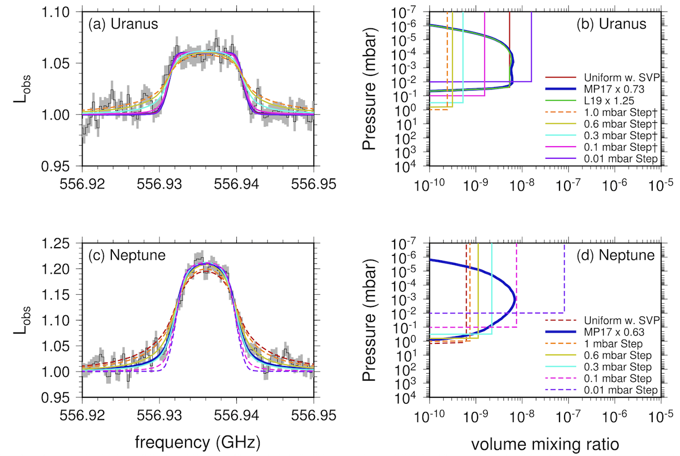
Fig2: Fits to Uranus and Neptune HIFI-HRS spectra 557GHz water line. (a,b) Uranus can be fitted with step profiles with a step pressure less than ~0.6mbar or by scaling photochemical profiles. However, significant water vapour is unlikely at pressures above ~0.03mbar due to saturation. (c,d) Neptune can be fitted with step profiles with a step in the pressure range 0.3-0.6mbar or by scaling photochemical profiles. (Figure from https://doi.org/10.3847/PSJ/ac650f, see reference [10]).
References
[1] Cavalié+ 2019. https://ui.adsabs.harvard.edu/abs/2019A%26A...630A..87C/abstract
[2] Feuchtgruber+ 1997. https://ui.adsabs.harvard.edu/abs/1997Natur.389..159F/abstract
[3] Lara+ 2019. https://ui.adsabs.harvard.edu/abs/2019A%26A...621A.129L/abstract
[4] Lellouch+ 2005. https://ui.adsabs.harvard.edu/abs/2005A%26A...430L..37L/abstract
[5] Levison 2000. https://ui.adsabs.harvard.edu/abs/2000Icar..143..415L/abstract
[6] Moreno+ 2017. https://ui.adsabs.harvard.edu/abs/2017A%26A...608L...5M/abstract
[7] Moses+Poppe 2017. https://ui.adsabs.harvard.edu/abs/2017Icar..297...33M/abstract
[8] Poppe 2016. https://ui.adsabs.harvard.edu/abs/2016Icar..264..369P/abstract
[9] Teanby+ 2019. https://ui.adsabs.harvard.edu/abs/2019Icar..319...86T/abstract
[10] Teanby+ 2022. https://ui.adsabs.harvard.edu/abs/2022PSJ.....3...96T/abstract
[11] Zahnle 2003. https://ui.adsabs.harvard.edu/abs/2003Icar..163..263Z/abstract
How to cite: Teanby, N., Irwin, P., Nixon, C., Cordiner, M., and Wright, L.: Uranus and Neptune's stratospheric water abundance and external flux from Herschel-HIFI, Europlanet Science Congress 2022, Granada, Spain, 18–23 Sep 2022, EPSC2022-168, https://doi.org/10.5194/epsc2022-168, 2022.
The past year has seen many papers underlining the significance of a space mission to Uranus and Neptune. Proposed mission plans usually involve a ~10 year cruise time to the ice giants. This cruise time can be utilized to search for low-frequency gravitational waves (GWs) by observing the Doppler shift caused by them in the Earth-spacecraft radio link. We calculate the sensitivity of prospective ice giant missions to GWs in comparison to former planetary missions which searched for GWs. Then, adopting a steady-state black hole binary population, we derive a conservative estimate for the detection rate of extreme mass ratio inspirals (EMRIs), supermassive- (SMBH) and stellar mass binary black hole (sBBH) mergers. For a total of ten 40-day observations during the cruise of a single spacecraft, approximately 0.5 detections of SMBH mergers are likely, if Allan deviation of Cassini-era noise is improved by ~102 in the 10−5 − 10−3 Hz range. For EMRIs the number of detections lies between O(0.1) − O(100). Furthermore, ice giant missions combined with the Laser Interferometer Space Antenna (LISA) would improve the GW source localisation by an order of magnitude compared to LISA by itself. With a significant improvement in the total Allan deviation, a Doppler tracking experiment might become as capable as LISA at such low frequencies, and help bridge the gap between mHz detectors and Pulsar Timing Arrays. Thus, ice giant missions could play a critical role in expanding the horizon of gravitational wave searches and maybe even be the first to detect the first SMBH merger.
How to cite: Soyuer, D., Zwick, L., D'Orazio, D., and Saha, P.: Ice Giant Missions as Gravitational Wave Detectors, Europlanet Science Congress 2022, Granada, Spain, 18–23 Sep 2022, EPSC2022-207, https://doi.org/10.5194/epsc2022-207, 2022.
Past years have seen numerous papers underlining the importance of a space mission to the ice giants in the upcoming decade. Proposed missions to Uranus and Neptune usually involve a ~10 year cruise time to the ice giants. In this phase, the spacecraft trajectories will mainly be determined by the configuration of massive bodies in the solar system. Interplanetary trajectories are monitored by recording Doppler shifts in the time series of the radio link between Earth and the spacecraft. The presence of dark matter (DM) affects the trajectory by introducing a small radial acceleration, which in turn reduces the velocity of the spacecraft over years of interplanetary travel. Additionally, bounds on the precession rate of ice giants could help constrain the local DM density and potentially rule out modified gravity scenarios.
We investigate the possibility of detecting the gravitational influence of DM in the solar system on the trajectory of prospective Doppler ranging missions to Uranus and Neptune, and also estimate the constraints such a mission can provide on modified and massive gravity theories via extra-precession measurements using orbiters around the ice giants.
The precision of these measurements is limited by the noise on the the two-way frequency fluctuation of the Doppler link. For the trajectory deviations, we developed a numerical procedure for reconstructing the influence of DM in the Doppler signal of thousands of simulated ice giant missions.
The noise improvements required to guarantee a local detection of dark matter in the early 2040s are realistic, provided they become one of the priorities during mission development.
How to cite: Zwick, L., Soyuer, D., and Bucko, J.: Prospects for a local detection of dark matter with future missions to Uranus and Neptune, Europlanet Science Congress 2022, Granada, Spain, 18–23 Sep 2022, EPSC2022-226, https://doi.org/10.5194/epsc2022-226, 2022.
Atmospheric probes provide a critical method for understanding the Ice Giants, offering unique insight into atmospheric composition, structure, and dynamics. Such in situ measurements are vital to understanding the formation and evolution of these bodies and our solar system. To pursue these scientific opportunities space agencies are now turning their attention to the developmemnt of atmospheric probes to the Ice Giants and other bodies. The newly released Decadal Survey prioritized Uranus and Saturn probes as well as a Venus in situ explorer. Few such missions have flown and it is not likely that there will be other atmospheric entry probes until the DAVINCI+ Venus probe mission in the early 2030’s. Entry probe concepts such as these require a delicate balance between science objectives, orbital mechanics, atmospheres, and signal processing. The development of future entry probe missions will rely on tools which allow mission teams to concurrently filter and compare trajectories to optimize science return.
To aid science planning for future entry probe missions we have developed a tool for Visualization of the Impact of PRobe Entry (VIPRE) conditions on science, mission and spacecraft design. VIPRE provides concurrent design capabilities for entry probe and lander missions by combining a precomputed database of optimized interplanetary trajectories with analytical models for entry point targeting, atmospheric descent and data-return rates. The user is able to explore the science trade-space using a GUI to constrain a variety of entry, trajectory, and data sufficiency parameters. Constraint-based interaction allows for direct, easy evaluation of scientific value and mission feasibility in real time. VIPRE is flexible to a variety of mission architectures allowing direct comparison of mission value between combinations of orbiters, entry vehicles and landers.
Users primarily interact with VIPRE through a GUI. Figure 1 provides an illustration of some of the available mission design, science parameter and constraint intereractions within the VIPRE GUI. On its left edge, the GUI allows for the selection of a target body, Saturn in this case, and a range of filtering parameters. Based on these inputs, the GUI displays the top row of plots which indicate the filtered interplanetary trajectory parameters. Once a trajectory of interest is selected the “Overview” parameters are populated and the bottom row plots are generated to illustrate reachable probe entry locations, colored based on parameters of interest. Reachability, in this case, is defined by the selected filtering parameters as well as target specific constraints, i.e. avoiding Saturn’s rings. The GUI also allows for user definition of figures and filter parameters, shown in this example under the "Globe" and "Side by Side" tabs.
This talk presents the motivation and models used for the development of VIPRE. Applications to Uranus and Saturn probe missions are discussed. Of particular interest is the accessibility of high and low latitudes for probe entry, how this is influenced by mission architecture (flyby versus orbiting probe release), and data constraints due to probe communications geometry.
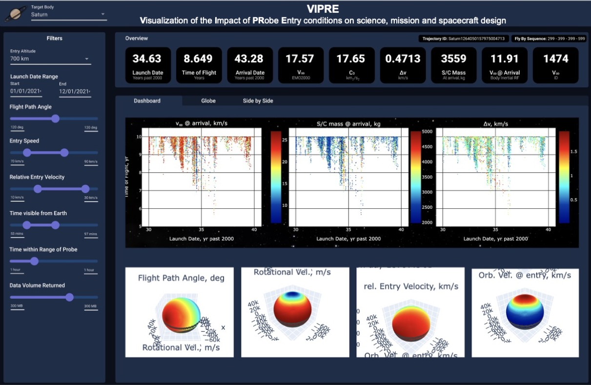
Figure 1. Example of VIPRE trajectory selection for a Saturn probe mission
[1] Probst, A. et al, VIPRE: A Tool Aiding the Design for Entry Probe Missions, The Planetary Science Journal 3.4 (2022) 98.
[2] Hofstadter, M. et al., Uranus and Neptune missions: A study in advance of the next planetary science decadal survey, Planetary and Space Science 177 (2019) 104680.
[3] National Academies of Sciences, Engineering, and Medicine. "Origins, Worlds, and Life: A Decadal Strategy for Planetary Science and Astrobiology 2023-2032." (2022).
How to cite: Davis, A., Landau, D., Atkinson, D., Hofstadter, M., Fedell, M., and Stonebreaker, R.: VIPRE: A Tool for Designing and Optimizing Science Return of Planetary Entry Probes, Europlanet Science Congress 2022, Granada, Spain, 18–23 Sep 2022, EPSC2022-262, https://doi.org/10.5194/epsc2022-262, 2022.
The ice giants Uranus and Neptune are the least understood class of planets in our solar system, while planets of their size, the most frequent among exoplanets, represent a common outcome of planet formation. Presumed to have a small rocky core, a deep interior comprising ~70% heavy elements surrounded by a more dilute outer envelope of H2 and He, Uranus and Neptune are fundamentally different from the better-explored gas giants Jupiter and Saturn. Because of the dearth of missions dedicated to their exploration, our knowledge of their composition and atmospheric processes is primarily derived from a single Voyager 2 flyby of each, complemented by subsequent remote sensing from Earth-based observatories, including space telescopes. As a result, Uranus's and Neptune's physical and atmospheric properties remain poorly constrained and their roles in the evolution of the Solar System are not well understood. Exploration of ice giant systems is therefore a high-priority science objective as these systems (which link together the magnetospheres, satellites, rings, atmosphere, and interior of these planets) challenge our understanding of planetary formation and evolution. In this context, the US planetary science decadal survey report recently recommended the launch of a flagship mission towards the Uranian system in the early 2030s. This mission would be composed of an orbiter aiming at exploring the Uranian system as a whole and a descent probe to directly sample the giant’s atmosphere.
Measurements to be made with a probe can be defined as Tier 1, representing threshold science required to justify the probe mission, and Tier 2 representing valuable science that significantly complement and enhance the threshold measurements, but of themselves are not sufficient to justify the mission. Tier 1 measurements comprise atmospheric noble gas abundances including helium, key noble gas isotope ratios, and the thermal structure of the atmosphere. Instrumentation required to achieve the Tier 1 measurements include a mass spectrometer, a helium abundance detector, and an atmospheric structure instrument comprising both sensors for pressure, temperature, a Tunable Laser System and atmospheric acoustic properties (speed of sound). Tier 1 science can be achieved with a probe making measurements near one to several bars. Tier 2 science includes measurements of key isotopic ratios, the abundances of atmospheric condensables and disequilibrium species, atmospheric dynamics, the net radiative flux transfer profile of the atmosphere, and the location, composition, properties, and structure of the clouds. To achieve all the Tier 2 science objectives requires a probe descending through at least ten bars carrying the full Tier 1 suite of instruments as well as a nephelometer, net flux radiometer, and an ultrastable oscillator to enable Doppler wind tracking of the probe throughout descent.
How to cite: Mousis, O. and Atkinson, D. H. and the Ice Giants team: Reference Science Payload for an Uranus Entry Probe, Europlanet Science Congress 2022, Granada, Spain, 18–23 Sep 2022, EPSC2022-572, https://doi.org/10.5194/epsc2022-572, 2022.
Background: The atmospheres of Uranus and Neptune are the most poorly constrained fluid atmospheres in the solar system. The ice giants were only visited, briefly, by the Voyager 2 spacecraft in the late 1980s. At Uranus, the Voyager 2 UV stellar and solar occultations detected a warm stratosphere and extremely hot thermosphere [1, 2], far in excess of heating caused by solar irradiance alone [3, 4]. Furthermore, Uranus has far smaller internal energy production than the other giant planets [5, 6] as well as a surprisingly well-equilibrated stratosphere given its 98º obliquity [7]. As the energy balance of Uranus’ atmosphere is unknown, it is often called the “Giant Planet Energy Crisis.”
Motivation and Aims: Between 1977 and 1998, dozens of stellar occultations by Uranus were observed from Earth (see [8] and references therein). In an Earth-based stellar occultation, stellar flux is diminished by differential refraction through the occulting atmosphere and is observed as a light curve. The original analyses of these light curves found cooler stratospheric and lower thermospheric temperatures than Voyager 2. Figure 1 shows the tension between the Earth-based and Voyager measurements of the upper atmosphere of Uranus. It is now possible to reprocess these archival light curves using modern techniques and better compare them to the Voyager 2 temperature profiles.
Methods: To reprocess the Earth-based stellar occultation light curves, we use a two-part procedure. We first fit the light curve to a smooth atmospheric model with power law temperature gradient [9] to set a boundary condition. We next perform inversion, which assumes ray optics, small bending angles, hydrostatic equilibrium, and an ideal gas to solve for temperature, pressure, and number density at each flux measurement [10]. This procedure has been significantly improved since the original data were published, allowing for non-isothermal boundary conditions, accurate uncertainties on output quantities, and much higher vertical resolutions [11].
In addition to producing atmospheric profiles from observed occultation light curves, we do the reverse by simulating Earth-based stellar occultation light curves using the Uranian temperatures reported by Voyager 2 [12]. We can then compare the generated light curves directly to our suite of observed ones.
Results: We present the temperature-pressure profiles from reanalysis of many archival Earth-based occultations and compare them to the published Voyager 2 findings. Further, we present the comparison of our synthetic Earth-based light curves, generated from a forward model of the Voyager 2 temperatures, to the observed Earth-based light curves. We comment on how consistent the Voyager 2 UV occultation findings are with Earth-based stellar occultation observations. Finally, we offer a revised Uranus temperature-pressure profile for the stratosphere and lower thermosphere based on these findings.
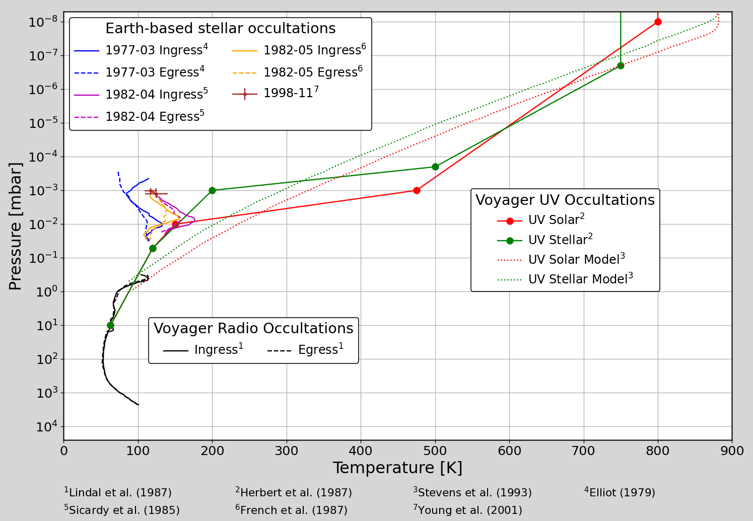
Figure 1. Comparison of remote sensing measurements of the atmosphere of Uranus. Earth-based occultations are blue [13], magenta [14], yellow [15] and brown [8]; Voyager UV occultations are solid red and green [1]; models are dotted red and green [2]; Voyager radio occultations are black [16]. Error bars are absent from this figure because they were not provided in the original publications.
References
[1] Herbert, F., et al. (1987). JGR, 92, pp. 15093–15109.
[2] Stevens, M. H., et al. (1993). Icarus, 101, pp. 45–63.
[3] Marley, M. S., and McKay, C. P. (1999). Icarus, 268-286.
[4] Li, C., Le, T., Zhang, X, and Yung, Y. (2018). J Quant Spectrosc Ra, 353–362.
[5] Pearl, J. C., Conrath, B. J., Hanel, R. A., Pirraglia, J. A, Coustenis, A. (1990). Icarus, 12-28.
[6] Bishop, J., et al. (1995). Neptune and Triton, pp. 427–487, University of Arizona Press.
[7] West, R. A., and Lane, A. L. (1987). JGR, 92, 30-36.
[8] Young, L. A., et al. (2001). Icarus, 153, pp. 236–247.
[9] Elliot , L. A., and Young, L. A. (1992). AJ, 991.
[10] Elliot, J. L., Person, M. J., & Qu, S. (2003). AJ, 126, 1041-1079.
[11] Saunders, W. R., Person, M. J., Withers, P. (2021). AJ, 161, 280.
[12] Chamberlain, D. and Elliot, J. (1997). PASP, 109, pp. 1170–1180.
[13] Elliot, J. L. (1979). Annu. Rev. Astron. Astrophys., 17, pp. 445-475.
[14] Sicardy, B., et al. (1985). Icarus, 64 pp.88-106.
[15] French, R. G., et al. (1987). Icarus, 69, pp. 499–505.
[16] Lindal, G. F. et al. (1987). JGR, 92, pp. 14987–15001.
How to cite: Saunders, W., Person, M., Withers, P., and French, R.: Uranus Upper-Atmospheric Temperatures From Stellar Occultations, Europlanet Science Congress 2022, Granada, Spain, 18–23 Sep 2022, EPSC2022-758, https://doi.org/10.5194/epsc2022-758, 2022.
Introduction
Our team has collected a 40+ year record of ground-based radio observations of Uranus, which constrain atmospheric circulation and chemistry in the 1 to 100 bar pressure region as a function of latitude, altitude, and season.
The Data Set
Our primary data set is 25 images of Uranus made at the Very Large Array (VLA) and Submillimeter Array (SMA) radio observatories between 1981 and 2022 (Fig. 1). Observations were made at wavelengths between 0.1 and 21 cm. They are augmented by unresolved measurements at wavelengths from 350 µm to 1.3 mm from the James Clerk Maxell Telescope (JCMT) and the Caltech Submillimeter Observatory (CSO).

Figure 1: VLA image of Uranus at a wavelength of 1 cm, observed in 2012. The North Pole is on the right. Bright regions have a lower abundance of absorbing species.
Retrievals of Atmospheric Properties
The data set is primarily sensitive to the vertical profiles of H2S, NH3, and H2O between about 0.7 and 100 bars (Fig. 2). We considered three models to constrain their vertical profiles.
Chemical Equilibrium Model: The abundance of species deep in the troposphere is allowed to vary with latitude, but vertically they are assumed to condense out according to their saturation vapor pressures. The saturation vapor pressure is allowed to be modified by a relative humidity anywhere from 0 to 10.
Hadley-Type Model: Low latitudes are in chemical equilibrium and represent regions of upwelling (Fig. 3). High latitudes represent areas of subsidence where condensable species are depleted down to a depth which is varied to fit the data.
Juno-Type Model: Inspired by results from the Juno spacecraft at Jupiter [1], all opacity is represented by NH3 with three free parameters: upper and lower atmospheric mixing ratios, and the pressure at which the transition between ratios occurs.
For all models that fit the data, we find:
- Regions poleward of ±50˚ are depleted in condensables relative to lower latitudes by a factor of ~50, down to a depth of ~20 to ~50 bars.
- Regions between the equator and ±30˚ are richer in condensables. Equilibrium models require more H2S in these regions than NH3.
- Regions between 30˚ and 50˚ North and South are intermediate in their abundance of condensables.
- In the 1 to 5 bar region, relative humidities at low latitudes are ~1.4 and they are ~0 over the poles, and/or the meridional temperature variations of ~ 2 K observed near 800 mbar [2] extend to these depths.
- The abundance of condensables over a large altitude range varies by ~30% near latitudes of 0˚, ±20˚ and ±75˚.
- During mid-summer the pole to equator contrast decreases.
Many of the features reported above have been seen previously [e.g., 3, 4], though our analysis is unique in spanning a large altitude and time range.
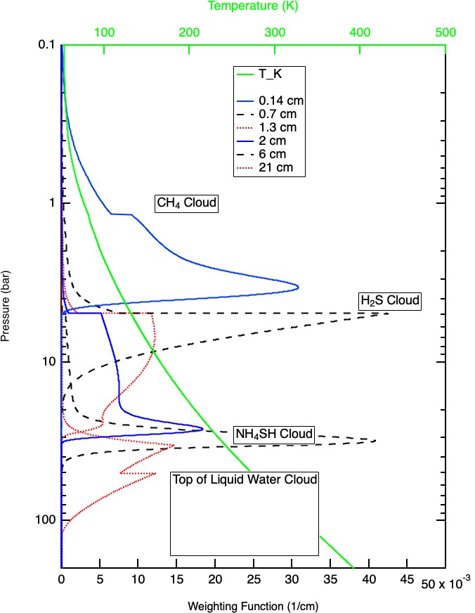
Figure 2: Weighting functions for the primary wavelengths used in this study, and the assumed atmospheric temperature profile. The location of various cloud layers is indicated.
Discussion
A large-scale circulation pattern is one possible cause of the observed spatial variations (Fig. 3). We refer to this as our Hadley-type model. (Uranus' poles receive more sunlight than the equator on an annual average, however, making this circulation opposite in a thermal sense to a classic Hadley cell.) At the time of the conference we expect to have completed dynamical modeling to test the plausibility of this scenario. In this model, smaller circulation patterns would explain the fainter banding seen in images (Fig. 1).
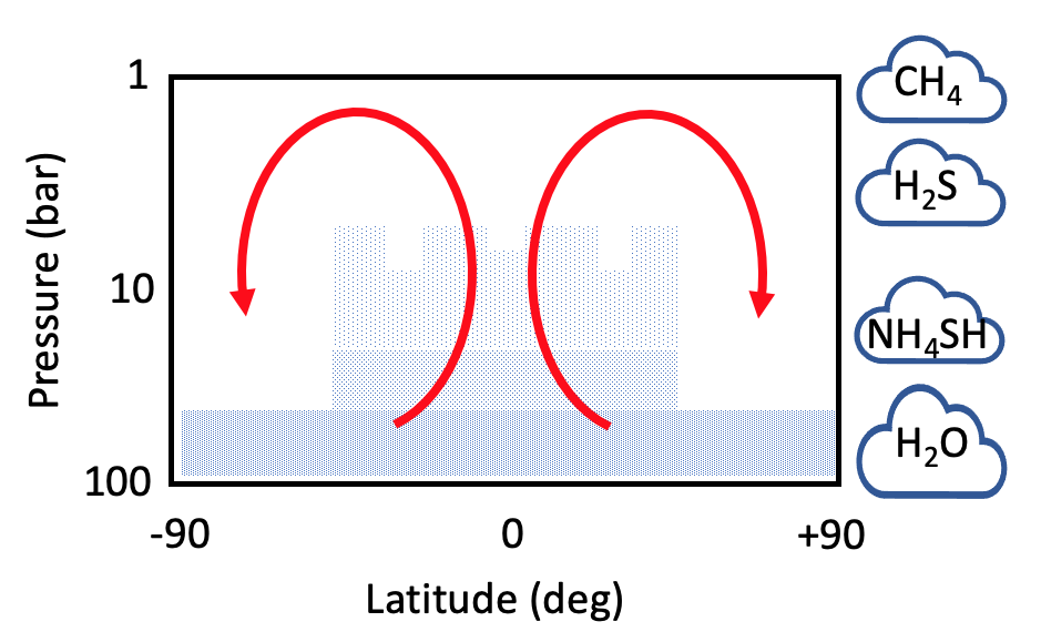
Figure 3: The density of blue dots is indicative of the observed absorber abundance. The altitude of expected clouds is shown along the right. A possible circulation pattern is indicated in red, with upwelling near the equator carrying absorber-rich air parcels upward. The rising air cools and clouds form, depleting air parcels in absorbers. Depleted air parcels then move poleward and descend at high latitudes.
An alternative explanation is what we refer to as a Juno-type model. The depletion of condensables in the ~5 to ~50 bar region of the Uranus atmosphere relative to deeper down and the meridional gradients are reminiscent of what the Juno spacecraft discovered at Jupiter [1]. Mechanisms proposed for Jupiter [e.g., 5] rely on vigorous convection. Since the variations at Uranus are more than 10x larger than those seen at Jupiter, but the uranian atmosphere near 1 bar seems less convectively active than Jupiter's, this interpretation would suggest that the deep Uranus troposphere is much more active than the upper troposphere. If such a process strongly depletes Uranus' 1 to 50 bar region of NH3 but depletes H2S to a lessor (but still significant) extent, that would explain why the observed absolute abundances of NH3 and H2S at Uranus are so much smaller than expected from planetary formation models, while the observed S/N ratio is much larger than expected [6].
The large-scale pole-to-equator brightness gradient and smaller-scale banding are always present in the spring, summer, and fall (the winter hemisphere cannot be seen from the Earth). For roughly ±5 years around the previous summer solstice (which occurred in 1985), however, the contrast between pole and equator was less than it was at other times, indicative of a weakening in circulation patterns. The next summer solstice is in 2028, so if we have indeed observed a seasonal effect, it should arise again in the next few years.
Acknowledgements
We thank the staff and funding agencies of the VLA, SMA, JCMT, and CSO observatories. We also thank Dr. Göran Sandell for providing the JCMT and CSO data used, and Dr.'s I. de Pater and E. Molter for useful discussions. Parts of this work were carried out at JPL/Caltech, under a contract with NASA.
References
[1] Bolton, S.J. et al. (2017) Science, 356, 6340/821. [2] Hanel, R.B. et al. (1986) Science, 233, 70–74. [3] Hofstadter, M.D. and Butler, B.J. (2003) Icarus, 165, 168–180. [4] Molter, E.M, et al. (2021) Plan. Sci Journ. 2:3. [5] Guillot, T. et al. (2020) JGR Planets, 125, e2020JE006403. [6] Atreya, S.K. et al. (2020) Space Sci Rev, 216:18.
How to cite: Hofstadter, M., Butler, B., Akins, A., Gurwell, M., and Friedson, J.: Radio Observations of Uranus: Implications for the Structure and Dynamics of the Deep Troposphere, Europlanet Science Congress 2022, Granada, Spain, 18–23 Sep 2022, EPSC2022-771, https://doi.org/10.5194/epsc2022-771, 2022.
How volatiles were incorporated in the building blocks of planets and small bodies in the protosolar nebula (PSN) remains an outstanding question. Some scenarios consider that planetesimals formed from a mixture of refractory material and volatiles trapped in amorphous ice in the outer nebula, while others hypothesize that volatiles have been incorporated in clathrates or formed pure condensates [1,2]. Here, we study the evolution of volatiles species in the PSN (H2O, CO, CO2, CH4, H2S, N2, NH3, Ar, Kr, Xe and PH3) considering two possible volatiles reservoir in the initial state: amorphous ice (see Figure 1) or pure condensates (see Figure 2). To do so, we use a 1D disk accretion model [3] with radial transport of trace species to compute the radial distribution of volatiles in the PSN. This model includes condensation/sublimation rates of pure condensates, as well as clathration/release rates when enough crystalline water is available. Figure 1 represents the case where volatiles are initially delivered to the PSN in the form of pure condensates. Figure 2 represents the case where volatiles are delivered to the PSN by amorphous ice. Species are released when amorphous grains cross the ACTZ region. Once delivered to the disk, the phase (solid or gaseous) of each species is ruled by the positions of its corresponding condensation and clathration lines. Clathration lines of the considered volatiles are closer to the Sun than their respective condensation lines, except for CO wich have its clathration line further from the sun than its condensation line. Gaseous volatiles condense or become entrapped (depending on the availability of water ice) when diffusing outward the locations of their lines. Conversely, volatiles condensed/entrapped in grains or pebbles are released in gaseous forms when drifting inward their lines. Peaks of abundances form close to each line. Our simulations show that a significant fraction of volatiles can be trapped in clathrates, only if they have initially been delivered in pure condensate forms to the disk. We also show that several regions in the protosolar nebula share a metallicity that is consistent with those measured in the atmospheres of the ice giants [3,4]. These findings have important implications for the formation history of the outer planets
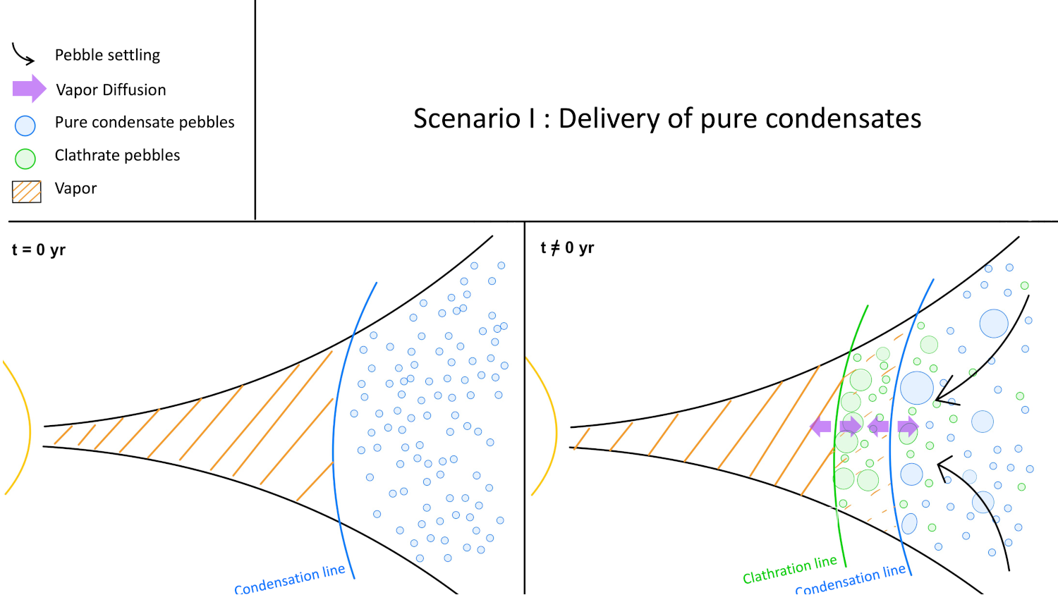
Figure 1 : Scheme showing the disk at initialization and at a given time. The volatiles are initially delivered under pure condensates and vapor. The vapor will condensate into clathrate hydrate, if there is enough crystalline water available. Grains drift inward while vapor undergo diffusion inward and outward. Leading to an accumulation of species at the place of condensation lines.
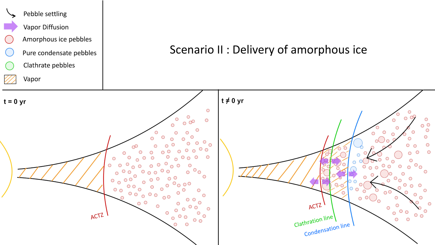
Figure 2 Scheme showing the disk at initialization and at a given time. The volatiles are initially delivered trapped into amorphous ice and vapor released from amorphous ice at the Amorphous to Crystalline Transition Zone (ACTZ). The clathration line is further than the ACTZ, since there no crystalline water after the ACTZ, clathration cannot happen, or is marginal if the clathration line is close to the ACTZ.
[1] : Gautier, D., Hersant, F., Mousis, O., et al. 2001, ApJL, 550, L227
[2] : Mousis, O., Ronnet, T., & Lunine, J. I. 2019, ApJ, 875, 9.
[3] : Aguichine, A., Mousis, O., Devouard, B., et al. 2020, ApJ, 901, 97.
[4] : Asplund, M., Grevesse, N., Sauval, A. J., et al. 2009, ARA&A, 47, 481.
[5] : Irwin, P. G. J., Toledo, D., Garland, R., et al. 2018, Nature Astronomy, 2, 420.
How to cite: Schneeberger, A., Mousis, O., Aguichine, A., and Lunine, J.: Evolution of the reservoir of volatiles in the protosolar nebula, Europlanet Science Congress 2022, Granada, Spain, 18–23 Sep 2022, EPSC2022-881, https://doi.org/10.5194/epsc2022-881, 2022.
Neptune's incomplete ring arcs have been stable since their discovery in 1984 by stellar occultation. Although these structures should be destroyed within a few months through differential Keplerian motion, imaging data over the past couple of decades have shown that these structures remain stable.
We present the first SPHERE near-infrared observations of Neptune's ring arcs taken at 2.2 μm (broadband Ks) with the IRDIS camera at the Very Large Telescope (VLT) in August 2016.
We derive accurate mean motion values for the arcs and the nearby satellite Galatea. The trailing arcs Fraternité and Égalité have been stable since they were last observed at VLT in 2007 (cf. Fig 1 left). Furthermore, we confirm the fading away of the leading arcs Courage and Liberté. Finally, we confirm the mismatch between the arcs' position and the 42:43 inclined and eccentric corotation resonances with Galatea, thus demonstrating that no 42:43 corotation model works to explain the azimuthal confinement of the arcs' material (cf. Fig. 1 right).
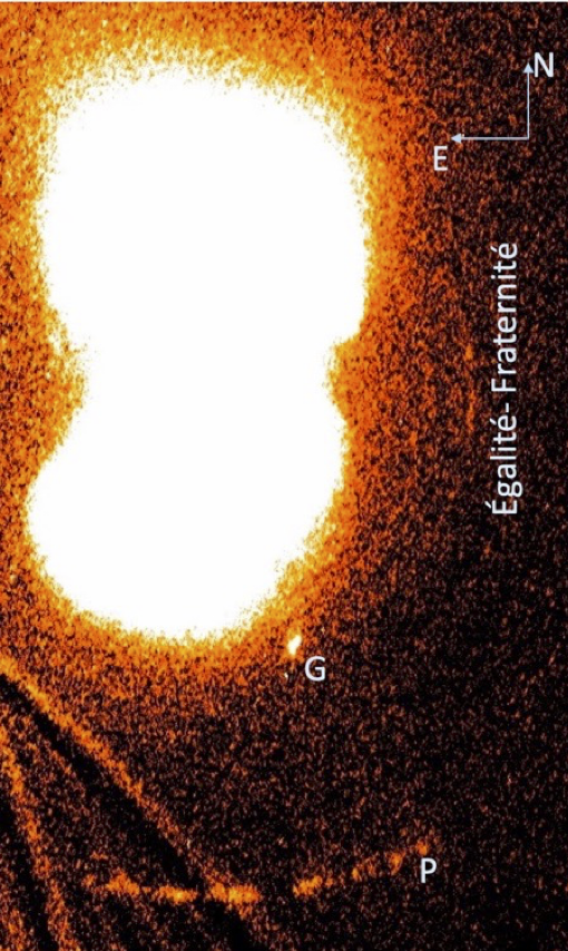
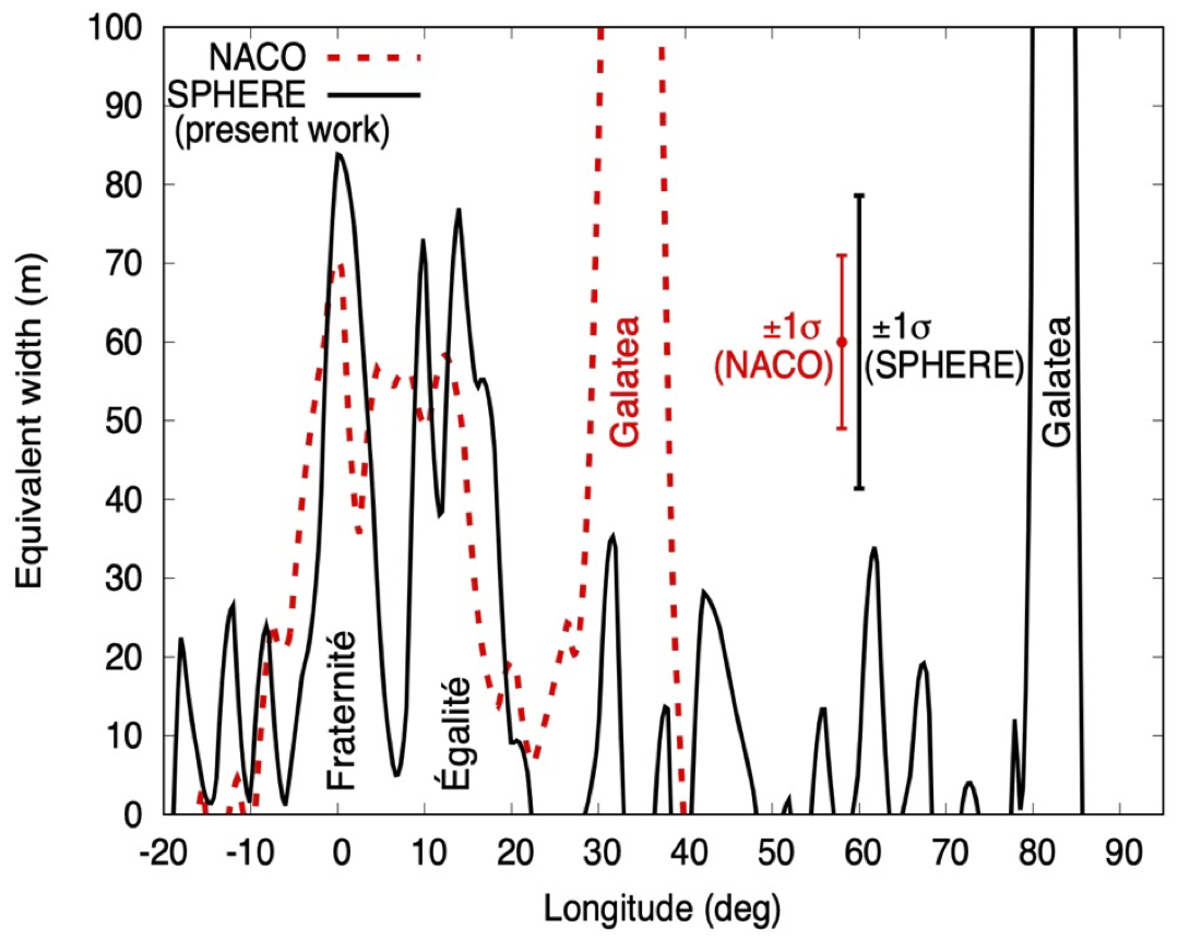
Fig. 1 (left) 68 projected and co-added images of Neptune’s equatorial plane, revealing material along the arcs Fraternité and Égalité, as well as the satellites Proteus (P) and Galatea (G). The frame is 7.1x10.7 arcsec2 wide. (right) Equivalent width of the arcs (Fraternité and Égalité), at an angular resolution of 2°. The X-axis origin is the longitude LFr of the centre of the Fraternité arc measured from the J2000.0 ascending node, where LFr = 217.43 deg, at the reference epoch. (Souami et al. 2022)
We also present here our NOC21 (Neptune stellar Occultation Campaign 2021) observational campaign to study the evolution of the Neptunian system since Voyager-2.
On October 7th, 2021, we led and organised the largest occultation and imaging campaign by the Neptunian system ever undertaken since the Voyager flyby in 1989. This occultation event was observable across the Americas (North and South) as well as in Hawaii, and the campaign involved all large telescopes in the region that were equipped with fast cameras either in the infra-red K band (2.2 μm) or in the visible using a CH4 filter at 890 nm. Combined with Adaptive Optics images, these observations will bring new constrains on Neptune's rings dynamics
We will use the occultation data collected during the NOC21 campaign along with AO data obtained at Keck observatory around the occultation time, to address the following points:
- the study of Neptune’s arcs’ system evolution using adaptive optics data,
- the detection of the main Le Verrier and Adams rings (see Fig.1) in the NOC21 data to measure their optical depths. In particular, we will search for possible changes in density of the Adams rings since the Voyager-2 mission in 1989,
- the search (in the NOC21 data) for any other narrow rings and/or small satellites and/or local debris such as arcs.
How to cite: Souami, D., Sicardy, B., Renner, S., and Langlois, M.: The evolution of Neptune’s arcs since Voyager-2. VLT/SPHERE observations of Neptune’s ring arcs and the 2021 Neptune stellar occultation campaign, Europlanet Science Congress 2022, Granada, Spain, 18–23 Sep 2022, EPSC2022-1263, https://doi.org/10.5194/epsc2022-1263, 2022.
OPS2 | Exploration of Titan
Introduction: Titan is an ocean world, an icy world, and an organic world. Recent models of the interior suggest that Titan’s subsurface ocean may be in contact with an organic-rich ice-rock core, potentially providing redox gradients, heavier elements, and organic building blocks critical for a habitable environment. Farther above, at the contact of the ice shell and ocean, Titan’s abundant surface organics could be delivered to the aqueous environment through processes such as potential convective cycles in the ice shell. Our work investigates the pathways for atmospheric organic products to be transported from the surface to the ocean/core and the potential for ocean/deep ice biosignatures and organisms to be transported to the shallow crust or surface for interrogation and discovery. Our major objectives are: (i) Determine the pathways for organic materials to be transported (and modified) from the atmosphere to surface and eventually to the subsurface ocean (the most likely habitable environment). (ii) Determine whether the physical and chemical processes in the ocean create stable, habitable environments. (iii) Determine what biosignatures would be produced if the ocean is inhabited. (iv) Determine how biosignatures can be transported from the ocean to the surface and atmosphere and be recognizable at the surface and atmosphere.
Summary of Progress: Examining Titan’s atmosphere, we have coupled two atmospheric models that cover different altitudes provide a comprehensive integrated model of the entire atmosphere of Titan. On the observational side, analysis of ALMA data resulted in the first observation of the CH3D molecule at sub-millimeter wavelengths [1]. Analysis of NASA IRTF data resulted in the first detection of propadiene (CH2CCH2) in Titan’s atmosphere [2]. Spatial and seasonal changes in Titan’s gases from the final years of the Cassini mission were the subject of several papers, using data from ALMA [3] and CIRS [4, 5]. In order to understand how materials falling from the atmosphere are transported across the surface, we are developing a landscape evolution model, based on the DELIM code that is used for Mars. We have published the first global geomorphologic map of Titan [6], which will serve as a constraint for the landscape evolution model by showing how sedimentary and depositional materials are distributed over the surface. We obtained an updated estimate of the amount of organic materials on Titan, which is important as a constraint on the amount of chemical energy and building blocks available for potential life. To investigate the molecular pathways from surface to subsurface ocean, we have performed a series of numerical simulations on the effect of a clathrate layer capping Titan’s icy crust on the convection pattern in the stagnant lid regime [7]. In the investigation of habitats resulting from molecular transport, we have modeled the accretion of Titan to understand the effects of thermal evolution on the rocky interior, and to constrain the composition of volatiles exsolved from the interior and that may have migrated vertically to build up the ocean early in Titan’s history [8]. We have also published results of modeling water-hydrocarbon mixtures using the CRYOCHEM code, which now successfully allows chemical modeling of both the hydrocarbon-rich condensed fluid phases and the water-rich condensed fluid phases (and vapor phases, too) simultaneously [9]. Preliminary results for our investigation of ocean habitats led to new insights into the origin of methane and nitrogen (N2) on Titan by modeling D/H exchange between organics and water, as well as high pressure C-N-O-H fluid speciation in Titan’s rocky core [10]. Results suggest an important role for organic compounds in the geochemical evolution of Titan’s core, which may feed into the habitability of Titan’s ocean. A novel experimental high pressure culturing chamber has been developed to investigate high pressure biosignatures which could survive in Titan’s ocean [11]. Our aim is to demonstrate that earth organisms can survive and build biomass in Titan’s subsurface conditions.
Acknowledgments: Part of this work was carried out at the Jet Propulsion Laboratory, California Institute of Technology, under contract with NASA. This work was funded by NASA’s Astrobiology Institute grant NNN13D485T.
References: [1] Thelen, A.E., et al. (2019) AJ, 157 (6), 219. [2] Lombardo, N.A., et al. (2019) ApJ Letters, 881: L3. [3] Cordiner, M.A., et al. (2019) AJ, 158:76. [4] Teanby, N. A. et al. (2019). GRL 46, 3079–3089. [5] Lombardo, N.A. et al. (2019): Icarus doi.org/10.1016/j.icarus.2018.08.027. [6] Lopes, R.M. (2020). Nature Astr., doi.org/10.1038/s41550-019-0917-6 [7] Kalousova K. and C. Sotin (2019) EPSC-DPS2019-288-1. [8] Neri, A., et al. (2020) Earth Planet. Sci. Lett., 530, 115920. [9] Tan, S. et al. (2019): ACS Earth 3, 11, 2569–258. [10] Miller, K.A. et al., (2019), Astrophys. J. 871, 59. [11] Russo, D., et al. (2021) AGU Fall Meeting.
How to cite: Lopes, R., Malaska, M., Steven, V., Hodyss, R., Meyer-Dombard, D., and Fagents, S. and the Titan NAI Team: Habitability of Hydrocarbon Worlds: Titan and Beyond, Europlanet Science Congress 2022, Granada, Spain, 18–23 Sep 2022, EPSC2022-45, https://doi.org/10.5194/epsc2022-45, 2022.
Titan, the largest satellite of Saturn, has a dense atmosphere mainly composed of nitrogen and methane at a percent level. These two molecules generate a complex prebiotic chemistry, a global haze, most of the cloud cover and the rainfalls which model the landscape. Methane sources are located in liquid reservoirs at and below the surface and it sink is the photodissociation at high altitude. Titan’s present and past climates strongly depend on the connection between the surface sources and the atmosphere upper layers. Despite its importance, very little information is available on this topic.
In the last two decades, the observations made by the Cassini orbiter and the Huygens probe have greatly improved our knowledge of Titan’s system. The surface, haze, clouds, and chemical species can be studied and characterised with several instruments simultaneously. On the other hand, some compounds of its climatic cycle remain poorly known. This is clearly the case of the methane cycle, which is, however, a critical component of Titan’s climate and of its evolution.
We reanalysed four solar occultations by Titan’s atmosphere observed with the infrared part of the Visual Infrared Mapping Spectrometer (VIMS) instrument. These observations were already analysed (Bellucci et al., 2009, Maltagliati et al., 2015), but here we used significantly improved methane spectroscopic data. We retrieved the haze properties (not treated previously) (Figure 1) and the mixing ratios of methane (Figure 2), deuterated methane, and CO in the stratosphere and in the low mesosphere.

Figure 1 : Haze extinction as a function of altitude, retrieved for the four observations, at wavelengths 0.884 μm (channel #97), 1.540 μm (channel #137) and 2.199 μm (channel #177). The extinction profiles retrieved by Seignovert et al. (2021) with Cassini/ISS, at wavelength 338 nm (CL-UV3 filters), are shown with green lines (labelled "S2020"). Those from Vinatier et al. (2010) or Vinatier et al. (2015), scaled at the wavelength 1μm, are shown with black lines ("V2010" or "V2015"). The profiles in cyan ("RP83"), are the extinctions retrieved by Rages & Pollack (1983) at 30◦N in August 1981 (wavelength 0.5 μm). The differences in the detached haze altitudes between VIMS-IR (Ls = 26°), Cassini/ISS (Ls = 14.8°) and Voyager 2/ISS (Ls = 18°) are their dates while the detached is falling down (West et al. (2018); Seignovert et al. (2021)). The grey line shows the haze profile by Doose et al. (2016) with DISR in 2005 at 10°S (labelled "D2016").
We find that the methane mixing ratio in the stratosphere is much lower (about 1.1%) than expected from Huygens measurements (about 1.4 to 1.5%). However, this is consistent with previous results obtained with CIRS. Features in the methane vertical profiles clearly demonstrate that there are interactions between the methane distribution and the atmosphere circulation. We find a layer rich in methane at 165 km and at 70°S (mixing ratio 1.45 ± 0.1%) and a dryer background stratosphere (1.1 − 1.2%). In absence of local production, this reveals an intrusion of methane transported into the stratosphere, probably by convective circulation. On the other hand, methane transport through the tropopause at global scale appears quite inhibited. Leaking through the tropopause is an important bottleneck of Titan’s methane cycle at all timescales. As such, it affects the long term evolution of Titan atmosphere and the exchange fluxes with the surface and subsurface reservoirs in a complex way.

Figure 2 : Methane mixing ratio retrieved with the four observation sets, with data between 0.88 and 2 μm (top) and between 2 and 2.8 μm (bottom). We also plot the methane mole fraction retrieved with the GCMS onboard Huygens (Niemann et al. (2010)) and with DIRS (Bézard (2014)) and CISR (Lellouch et al. (2014)). The green dashed profile, in the upper left graph, shows the evaluation made by Rannou et al. (2021).
We also retrieved the haze extinction profiles and the haze spectral behaviour. We find that aerosols are aggregates with a fractal dimension of Df ≃2.3±0.1, rather than Df ≃2 as previously thought. Our analysis also reveals noticeable changes in their size distribution and their morphology with altitude and time. These changes are also clearly connected to the atmosphere circulation and concerns the whole stratosphere and the transition between the main and the detached haze layers.
We conclude that, to fully understand these results, Global Climate Models accounting for haze and cloud physics, thermodynamical feedbacks and convection are needed. Especially, the humidificaton of the stratosphere, at the present time and its evolution under changing conditions at geological timescale appears as a key process, and our work provide strong constraints to guide studies.
References
Bellucci, A., Sicardy, B., Drossart, P., et al. 2009, Icarus, 201, 198
Bézard, B. 2014, Icarus, 242, 64
Doose, L. R., Karkoschka, E., Tomasko, M. G., & Anderson, C. M. 2016, Icarus, 270, 355
Lellouch, E., Bézard, B., Flasar, F. M., et al. 2014, Icarus, 231, 323
Maltagliati, L., Bézard, B., Vinatier, S., et al. 2015, Icarus, 248, 1
Niemann, H. B., Atreya, S. K., Demick, J. E., et al. 2010, Journal of Geophysical Research (Planets), 115, E12006
Rages, K. & Pollack, J. B. 1983, Icarus, 55, 50
Rannou, P., Coutelier, M., Riviere, E., et al. 2021, Astrophysical Journal, 922
Rey, M., Nikitin, A., Bézard, B., et al. 2018, Icarus, 303, 114
Seignovert, B., Rannou, P., West, R. A., & Vinatier, S. 2021, The Astrophysical Journal, 907, 36
Vinatier, S., Bézard, B., de Kok, R., et al. 2010, Icarus, 210, 852
Vinatier, S., Bézard, B., Lebonnois, S., et al. 2015, Icarus, 250, 95
West, R. A., Balloch, J., Dumont, P., et al. 2018, Geophysical Research Letters, 38
How to cite: Rannou, P., Coutelier, M., Lebonnois, S., Maltagliati, L., Rivière, E., Rey, M., and Vinatier, S.: Solar occultations observed by VIMS-IR: What haze and methane profiles reveal about Titan's atmospheric dynamics and climate., Europlanet Science Congress 2022, Granada, Spain, 18–23 Sep 2022, EPSC2022-130, https://doi.org/10.5194/epsc2022-130, 2022.
Molecular nitrogen (N2) and methane (CH4) are the two major gas of Titan’s atmosphere. Their dissociation in the upper atmosphere by photons and photo-electrons leads to a wealth of chemical reactions forming more complex molecules like nitriles and hydrocarbons, which subsequently combine to form Titan’s photochemical haze.
Isotopic ratios measured in N2 and CH4 are of particular interest to constrain the origin and evolution of Titan’s atmosphere. While the same isotopic ratios measured in photochemical species bring constraints on fractionation processes occurring through their formation and/or loss.
We focus on the determination on the 14N/15N and the 12C/13C isotopic ratios in HCN and the 12C/13C ratio in HC3N by analyzing their thermal emission acquired by the Cassini Composite Infrared Spectrometer (CIRS) from 2004 to 2017 (from the northern winter to the northern summer). We used the entire CIRS dataset acquired with a limb-geometry viewing at the highest spectral resolution (0.5 cm-1). This allows us to search for potential variations of these isotopic ratios with latitude or with season, which could help to identify potential fractionation processes. Our analysis incorporates the temperature and minor species volume mixing ratio profiles inferred previously by Mathé et al. (2020) from the same limb dataset. We will present our results regarding the isotopic ratios in HCN for all latitudes, while we will present the 12C/13C ratio in HC3N only at high latitudes, as this nitrile is not detected at mid- and low-latitudes.
References:
- Mathé et al., 2020. Seasonal changes in the middle atmosphere of Titan from Cassini/CIRS observations: Temperature and trace species abundance profiles from 2004 to 2017. Icarus 344, id. 113547.
How to cite: Vinatier, S., Mathé, C., Bézard, B., Jolly, A., and Gautier, T.: Isotopic ratios in Titan’s HCN and HC3N derived from Cassini/CIRS observations, Europlanet Science Congress 2022, Granada, Spain, 18–23 Sep 2022, EPSC2022-258, https://doi.org/10.5194/epsc2022-258, 2022.
We present a study of the methane abundance in Titan's lower stratosphere. We analyzed spectra of Titan's atmosphere in the mid- and far-infrared region recorded by the Composite Infrared Spectrometer (CIRS) aboard the Cassini spacecraft with nadir geometry to determine the methane mixing ratio between 1 and 20 mbar range and its variations with seasons and latitudes.
Lellouch et al. (2014) analyzed CIRS observations recorded over the first part of the Cassini-Huygens mission, from August 2005 to June 2010, during Titan's northern winter and early spring. They showed that the methane mole fraction in Titan's atmosphere varies with latitudes from about 1.0% to 1.5%, which was unexpected as, due to its long chemical lifetime, CH4 is supposed to be homogenized by the atmospheric circulation.
The goal of this study is to analyze Cassini/CIRS data taken over the last part of the mission during northern spring and early summer (June 2010 to September 2017) in order to retrieve CH4 mixing ratio, vertical profiles of temperature and aerosols opacity at the 19 latitudes that we have selected. We analyzed spectra acquired by two focal planes of CIRS (FP1 and FP4) covering the spectral range from 10 to 600 cm-1 and from 1050 to 1500 cm-1, respectively. FP1 spectra include emission from CH4 pure rotational lines and FP4 spectra include the CH4 ν4 band centered at 1305 cm-1. We use an iterative process to determine the temperature profile from the tropopause (using the FP1) to the low stratosphere (using the FP4) by fitting the continuum of the FP1 spectra in the 70-150 cm-1 wavenumber range and the CH4 ν4 band in the 1200-1350 cm-1 range. The obtained thermal profile is used to retrieve the methane mole fraction by fitting their rotational lines in the 75-150 cm-1 range. We use the obtained value as a priori of a new iteration (retrieving the temperature profile and the CH4 mole fraction subsequently). Convergence is obtained after a few iterations.
We will present the derived CH4 mixing ratios during the northern spring and compare them with the results of Lellouch et al. (2014), which mostly focused on the northern winter. This will allow us to derive potential seasonal variations that could occurred after the global circulation overturning during the spring.
Reference :
- Lellouch et al. (2014). The distribution of methane in Titan’s stratosphere from Cassini/CIRS observations. Icarus 231, 323-337.
How to cite: Houelle, M., Vinatier, S., Bézard, B., and Lellouch, E.: The distribution of methane in Titan's atmosphere during northern spring from Cassini/CIRS observations, Europlanet Science Congress 2022, Granada, Spain, 18–23 Sep 2022, EPSC2022-410, https://doi.org/10.5194/epsc2022-410, 2022.
The Cassini/UVIS observations of Titan’s atmosphere extend from 2005 to 2017 providing a broad spatial and temporal view of the upper atmosphere including the seasonal change from Southern summer at the Cassini-Huygens arrival in 2005, to equinox (August 2009), to Northern summer (summer solstice in May 2017). The general emission characteristics of the illuminated Titan side are common among the observations: Near the ionospheric peak (~1100 km) the atomic and molecular emissions dominate the observed signal (Fig. 1). Atomic emissions include Ly-α (1216.7 Å) scattering from atomic hydrogen and emissions from N and N+ excited during the photolysis of N2, with major contributions at 1085 Å (N+, 3D0 à 3P), 1200 Å (N, 4D0 à 4S0 ) and 1493 Å (N, 2P à 4S0). Molecular emissions are dominated by the Lyman-Birge-Hopfield (LBH, α 1Πg à X 1Σg+) and Vegard-Kaplan (VK, A3Σu+ à Χ 1Σg+) bands, both in the FUV. These observations provide valuable constraints for the atmospheric structure.
We use a detailed forward model to simulate the observed emission, which relies on constraints from models of solar energy deposition (Lavvas et al. 2011) and N2 aiglow (Lavvas et al. 2015). Our simulations demonstrate that all observed emissions result from the excitation of atomic and molecular nitrogen and from scattering by atomic hydrogen (Fig. 1). Using such a detailed forward model for the inversion of the atmospheric properties is, however, inefficient due to the large computational times involved. Instead we propose a simplified retrieval focusing on specific atomic lines in the FUV range, which allows for an efficient atmospheric characterization with minimal computational effort, while preserving the benefits of the detailed forward modeling.
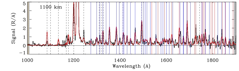
Figure 1: Observed (black) and simulated (red) limb spectra on Titan’s dayside during the 2016, DOY-015 PRIME observations. The top panel presents the average spectrum at 1100 km (100 km wide bin) demonstrating the strong Ly-α emission and the emissions from atomic (dashed lines) and molecular transitions (thin blue lines for LBH and thin red lines for VK bands).
References
- Lavvas P., Yelle R.V., Heays A.N., Campbell L., Brunger M.J., Galand M., Vuitton V., 2015. N2 state population in Titan’s atmosphere. Icarus, 260, p.29-59.
- Lavvas P., Galand M., Yelle R.V., Hayes A.N., Lewis B.R., Lewis G.,R. Coates A.J., 2011. Energy deposotion and primary chemical products in Titan’s atmosphere. Icarus, 213, 233-251.
How to cite: Lavvas, P. and Koskinen, T.: Titan’s atmospheric structure from Cassini/UVIS airglow observations, Europlanet Science Congress 2022, Granada, Spain, 18–23 Sep 2022, EPSC2022-447, https://doi.org/10.5194/epsc2022-447, 2022.
Introduction
With 13 years of observations, the Visual And Infrared Mapping Spectrometer (VIMS) onboard the \textit{Cassini} spacecraft has observed the surface and atmosphere of Titan through two seasons: winter and spring. In VIMS-IR spectra the surface is only seen in seven atmospheric windows due to the strong methane absorption. To retrieve the surface albedo we use radiative transfer (RT) models to compensate for the signal due to the atmosphere. Thanks to the lander Huygens, we have information about the optical properties of the aerosols above the equator that can be used in RT models. However, using the same aerosols vertical profile at high latitude doesn't work. With the help of the results of and Global Circulation Models and the Composite InfraRed Spectrometer onboard Cassini, we changed the aerosol vertical profile and optical properties in our RT model to better fit VIMS data at high latitude. While this model is not well constrained due to a lack of data, we manage to adjust the optical properties so our RT model based on Coutelier et al., (2021) retrieve surface albedo mostly between 0 and 1 instead of values crossing these boundaries like we had previously. It allow us to study with a RT model the shores and polar seas of Titan. We applied this new model on the same area of Kraken Mare in three consecutive VIMS cubes of the same flyby (subsequently named C1, C2 and C3). It allow us to validate our model on terrains with different albedo, and to notice an interesting feature in Kraken Mare that could be interpreted as sediment transport into the sea.
Adaptation of the aerosols optical properties and vertical profile
We decided to keep a 2 layers-based aerosol model, separated into haze and mist. We first changed the haze opacity vertical profile, using an exponential law : 
with the altitude of transition between mist and haze Ztr=70 km, and the scale height Hh=40 km. τh1µm is the opacity calculated by Doose et al., 2016 at 1 µm. We then changed the spectral slope of the optical depth of the mist with a simple power law as a first approximation :

with Δτmnorm the normalized optical depth of the atmospheric layer of mean altitude z, τhλ0 the total optical depth at λ0 = 1 µm calculated by Doose et al 2016., λ the wavelength, and the parameter b = 2.2 +/- 0.2
The most influent parameter is the mist single scattering albedo ωm. we decided to change it depending on that of the haze ωh and a factor α = 0.4 +/- 0.1.

Application and results on Kraken Mare
We tuned and applyed this model on three successive VIMS cubes (full names in Fig. 1) subsequently called C1, C2 and C3. We retrieved the albedo on a zone crossing Kraken Mare, containing pixels from land, shore and methane sea. They are circled in red in Fig.1. The top part shows the VIMS cubes, and the bottom part their footprint on the geomorphologic map of Titan. That way we can have an expectation on the retrieved albedo: dark in the sea, and bright on land.
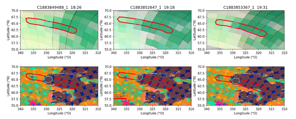
Figure 1 : (top) Successive VIMS cubes from flyby 292TI (colors : R : 5.01, V : 1.28, B : 2.79 μm).(bottom) : Footprint of the VIMS pixels on the geomorphologic map from Lopez et al., 2020. The pixels in our study are circled in red. The pixels circled in blue have mixed signatures.
The retrieved albedo are on Fig. 2. We still have remaining problems with negative albedo on dark pixels, mostly in the first atmospheric window. We can still differentiate very well the signatures from different terrains. Those coming from Kraken Mare are in blue, and those coming from the land are in green in Fig. 2. In C2, we have a pixel localized on the shore containing part of land and sea, circled in pink. Its signature is mixed, as we expected. However, we notice that on C1 and C3, two pixels localized in Kraken Mare (also circled in pink) also have a mixed signature. We did check that it was not a mistake in the cube geolocalization, or a difference due to a cloud.
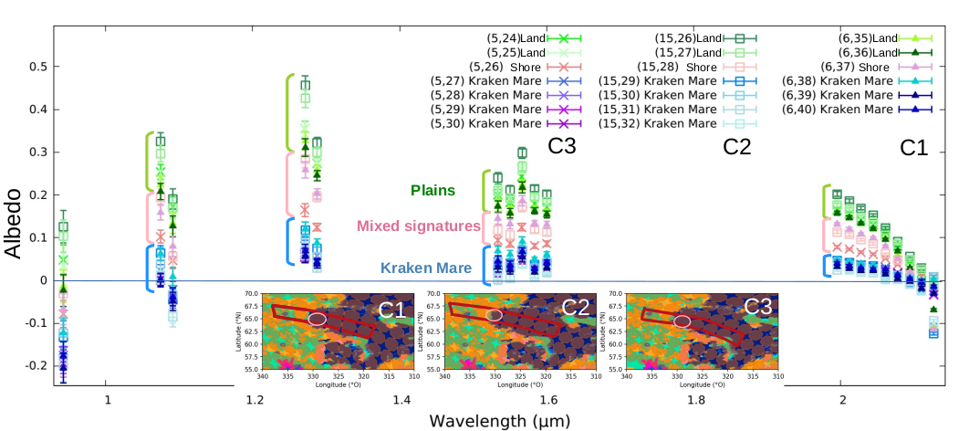
Figure 2 : Retrieved albedo of the selected pixels in Fig. 1. from the cubes C1, C2 and C3. The errors bar are calculated from the error on VIMS, and not from the error on the model. They are underestimated as a consequence.
Discussion
Infrared can penetrate deeply into liquid methane and ethane. The mixed signature we noticed can come from sediment transport carried by rivers flowing into Kraken Mare, issued from the erosion of the bedrock.
While this aerosol model for the poles is not exact, nor well constrained, the RT model is working and gives reasonable results on different cubes from the same flyby. We can compare the different surface albedos instead of the absolute values, because the atmospheric model is the same for all of the studied pixels. The combination of the RT analysis with the geomorphologic map is a powerful tool that leads to notice unexpected signatures.
With the seasons changes, we can expect that the improved polar aerosol model is not constant, so further studies should be made on other cubes through different seasons. We could that way follow through an other method the seasonal variation of the polar haze and mist layers.
References
Doose et al. (2016) Vertical structure and optical properties of Titan’s aerosols from radiance measurements made inside and outside the atmosphere. Icarus 270 : 355-375.
Coutelier et al. (2021) Distribution and intensity of water ice signature in South Xanadu and Tui Regio. Icarus 364 : 114464.
Lopes et al. (2020) A global geomorphologic map of Saturn’s moon Titan." Nature astronomy 4.3 : 228-233.
How to cite: Coutelier, M., Rannou, P., Cordier, D., and Seignovert, B.: Detection of sediment transport in Kraken Mare with a radiative transfert model using an aerosol vertical profile and optical properties adapted to Titan North pole, Europlanet Science Congress 2022, Granada, Spain, 18–23 Sep 2022, EPSC2022-449, https://doi.org/10.5194/epsc2022-449, 2022.
1. Introduction
Titan is the only moon in our solar system with a substantial atmosphere. It comprises 98% Nitrogen (Niemann et al., 2005), and is rich in hydrocarbon (CxHy) and nitrile (CxHyNz) species. Such species photochemically react to produce organic aerosols which compose a thick orange haze suspended in Titan’s middle atmosphere.
Global Circulation Models (GCMs) predict the meridional circulation in Titan’s stratosphere and mesosphere is dominated by a single pole-to-pole circulation cell for most of the Titan year (Hourdin et al., 1995; Newman et al., 2011; Lebonnois et al., 2012), and observations are broadly consistent with this prediction (Teanby et al., 2012, Vinatier et al., 2015). These models suggest circulation across the stratospheric equator, but this is not entirely consistent with what is observed. Existing studies show a North-South asymmetry in stratospheric haze abundance (Lorenz et al., 1997; de Kok et al., 2010), suggesting a mixing barrier near the equator. Here, we present a radiance ratio method for approximating latitudinal distributions of stratospheric HCN. We apply this to the region +/-30 degN and use HCN as a tracer to investigate the evolution and behaviour of the equatorial mixing barrier over the Cassini mission.
2. Observations
The Cassini spacecraft explored Saturn and its moons from 2004 to 2017. Throughout its 13-year exploration, Cassini performed 127 close flybys of Titan, observing at infrared, visible and ultra-violet wavelengths. One of Cassini’s twelve instruments, the Composite Infrared Spectrometer (CIRS) (Flasar et al., 2004; Jennings et al., 2017; Nixon et al., 2019) collected almost 10 million Titan spectra in the mid and far-infrared ranges (10 – 1500 cm-1), at a varied spectral resolution between 0.5 – 15.5 cm-1. In this study, we analyse low spectral resolution (~15 cm-1) observations collected by two CIRS focal planes, sensitive to wavenumber ranges 600 – 1100 cm-1 (FP3) and 1100 – 1500 cm-1 (FP4). Generally, low spectral resolution observations require shorter scan times so can be performed at a closer approach distance to Titan, hence achieving higher spatial resolution. This allows small spatial variations in atmospheric constituents to be resolved. Low-resolution observations also have good coverage of Titan’s equatorial region throughout the entire Cassini mission (Figure 1).
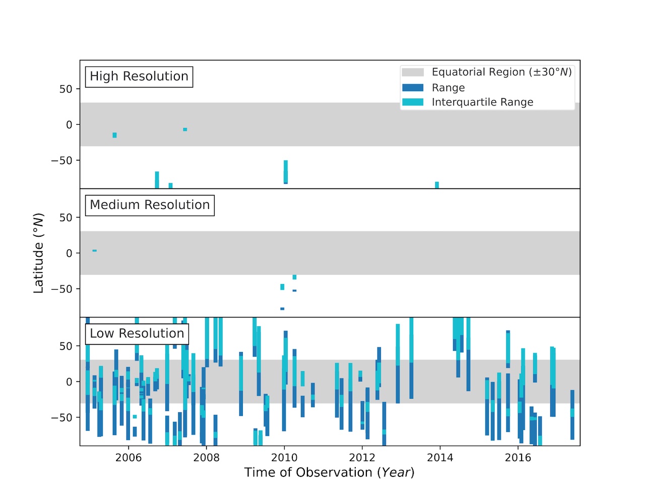
Figure 1: Mission coverage for the Cassini CIRS low spectral resolution nadir mapping observations.
3. Optimising Line-by-Line Retrieval Efficiency
Line-by-line (LBL) inversions in spectral analysis are computationally expensive. The correlated-k approximation (Lacis and Oinas, 1991) is often used to decrease the computation time of retrievals, but we found that it is not sufficiently accurate for these low spectral resolution and high signal-to-noise ratio observations (Figure 2c, d). In LBL modelling, a key parameter is the underlying spectral grid spacing. Finer grid spacing improves the forward model accuracy, but at a greater computation cost. To improve the efficiency of LBL runs, we determine a maximum grid spacing (Figure 2a, b) for which a LBL inversion will produce a sufficiently accurate spectrum in the shortest computation time. Typically, a single forward model run takes 2 hours for LBL, compared to 2 seconds for k-tables.
Figure 2: Comparison of spectra produced using a correlated-k (k-table) method and a line-by-line (LBL) method at varied spectral grid spacing. Maximum radiance difference (MRD) (a, b, blue line) between spectra produced at varied (0.1 – 0.0001 cm-1) and fine (0.0001 cm-1) grid spacing is assessed against a level of sufficient accuracy (a, b, grey area). The grid spacing determined to be optimal (0.001 cm-1 for FP3, 0.005 cm-1 for FP4) produces an almost identical spectrum to very fine (0.0001 cm-1) grid spacing (c, d) but at a significantly reduced runtime (a, b). A spectrum produced using a coarse grid spacing (0.1 cm-1) is shown for comparison. The spectrum retrieved using k-tables is not sufficiently accurate for these low-resolution observations (c, d).
4. Estimating Stratospheric HCN with a Radiance Ratio
We construct a radiance ratio formula for approximating HCN abundance from CIRS spectra, such that a greater number of observations can be analysed rapidly. Radiance ratios can be a useful tool for approximating gas contributions to a spectrum. They do not have the reliability of full spectral retrievals but require significantly less computation time. We compare the radiance ratio latitude dependence to full LBL retrievals of HCN, for a subset of our observations, to assess the reliability of our ratio method. LBL retrievals are performed using the Nemesis radiative transfer and retrieval code (Irwin et al., 2008) with our pre-determined optimal grid spacing. We calculate the radiance ratio for a set of approximately 20 low spectral resolution mapping observations (3 are shown in Figure 3).
There appears to be a sharp change in HCN abundance near the equator (Figure 3). This hints at a potential mixing barrier in Titan’s stratosphere. Furthermore, the position of this potential barrier appears to migrate over time. We use the results of this study to investigate dynamic processes in the equatorial region of Titan’s stratosphere and its evolution over the entire Cassini mission.
Figure 3: Our radiance ratio calculated for observations acquired on 08/2005 (a), 05/2006 (b) and 07/2012 (c). The radiance ratio is smoothed by fitting splines (Teanby, 2007). The gradient of each smoothed fit is also shown (bottom).
Acknowledgements
This research was funded by the UK Sciences and Technology Facilities Council.
References
de Kok, R., et al. (2010). https://doi.org/10.1016/j.icarus.2009.10.021
Flasar, F. M., et al. (2004). https://doi.org/10.1007/s11214-004-1454-9
Hourdin, F., et al. (1995). https://doi.org/10.1006/icar.1995.1162
Irwin, P., et al. (2008). https://doi.org/10.1016/j.jqsrt.2007.11.006
Jennings, D. E., et al. (2017). https://doi.org/10.1364/AO.56.005274
Lacis, A. A., & Oinas, V. (1991). https://doi.org/10.1029/90JD01945
Lebonnois, S., et al. (2012). https://doi.org/10.1016/j.icarus.2011.11.032
Lorenz, R. D., et al. (1997). https://doi.org/10.1006/icar.1997.5687
Newman, C. E., et al. (2011). https://doi.org/10.1016/j.icarus.2011.03.025
Nixon, C. A., et al. (2019). https://doi.org/10.3847/1538-4365/ab3799
Niemann, H. B., et al. (2005). https://doi.org/10.1038/nature04122
Teanby, N. A. (2007). https://doi.org/10.1007/s11004-007-9104-x
Teanby, N. A., et al. (2012). https://doi.org/10.1038/nature1161
Vinatier, S., et al. (2015). https://doi.org/10.1016/j.icarus.2014.11.019
How to cite: Wright, L., Teanby, N. A., Irwin, P. G. J., Nixon, C. A., and Mitchell, D. M.: Stratospheric HCN and Evolution of a Mixing Barrier in Titan’s Equatorial Region from Low-Resolution Cassini/CIRS Spectra, Europlanet Science Congress 2022, Granada, Spain, 18–23 Sep 2022, EPSC2022-463, https://doi.org/10.5194/epsc2022-463, 2022.
Introduction
With 13 years of observations, the Ion and Neutral Mass Spectrometer (INMS) onboard the Cassini spacecraft has observed the upper atmosphere of Titan through two seasons: winter and spring. The complex atmosphere is mainly composed of N2, CH4, H2 and Ar, but a lot more carbon and nitrogen bearing trace species have been observed by INMS and other instruments. Using data from the closed source neutral mode of INMS instrument, we studied the abundance and variation of traces neutral species in Titan ionosphere, between 1500 and 950 km of altitude. We will present an ongoing effort on the reanalysis of the entire INMS Titan's observation dataset.
Method
To do so we recalibrated INMS data by taking into account the dead time correction, the ram pressure enhancement, the saturation correction, the increase of pressure in the chamber with the decreases of altitude, the sensitivity and the contamination by thruster firing (Cui et al., 2009,2012). In addition, species entering the instrument were ionized and fragmented into ions inside INMS chamber, making difficult the identification of different species in such complex mass spectra. To retrieve the molecular mixing ratios we used a Monte-Carlo sampling on the fragmentation pattern to deconvolve the signal. To obtain a complete mass spectrum (m/z 1 to 99), we stacked INMS data, which increases the incertitude on the altitude. We used the mass spectra deconvolution code developed by Gautier et al., (2020), also employed by Serigano et al., (2020) when they treated Saturn INMS data.
This enabled the retrieval of vertical and seasonal variation of Titan's atmosphere minor components. We expect to be able to link our results with the seasonal variations observed by other instruments [such as CIRS (Mathé et al., 2020)] in lower atmospheric layers.
References
Cui et al.(2009) Analysis of Titan’s neutral upper atmosphere from Cassini Ion Neutral Mass Spectrometer measurements. Icarus 200 (2009) 581–615
Cui et al.(2012) The CH4 structure in Titan’s upper atmosphere revisited. J. Geophys. Res., 117, E11006, doi:10.1029/2012JE004222.
Gautier et al. (2020) Decomposition of electron ionization mass spectra for space application using a Monte-Carlo approach. Rapid. Com. Mass Spec. 34(8), e8659
Mathé et al., (2020) Seasonal changes in the middle atmosphere of Titan from Cassini/CIRS observations: Temperature and trace species abundance profiles from 2004 to 2017. Icarus, 344, 113547.
Serigano et al. (2020) Compositional measurements of saturn's upper atmosphere and rings from cassini INMS. Journal of Geophysical Research: Planets, 125(8), e2020JE006427.
How to cite: Coutelier, M., Gautier, T., Das, K., Serigano, J., and Horst, S.: Seasonal variation of trace species in Titan’s ionosphere, Europlanet Science Congress 2022, Granada, Spain, 18–23 Sep 2022, EPSC2022-479, https://doi.org/10.5194/epsc2022-479, 2022.
Introduction
Titan is the only moon in the solar system with a thick atmosphere, dominated by nitrogen and organic compounds and methane- and ethane-based climatic cycles similar to the hydrological cycle on Earth. Hence, Titan is a prime target for planetary and astrobiological researches. Heaviest organic materials resulting from atmospheric chemistry (including high atomic number aerosols) precipitate onto the surface and are subject to geological processes (e.g., eolian and fluvial erosion) that lead to the formation of a variety of landscapes, including dune fields, river networks, mountains, labyrinth terrains, canyons, lakes and seas analogous to their terrestrial counterparts but in an exotic context. Its optically thick atmosphere, however, prevents the surface from being probed in the entirety of the near-infrared (NIR) range, and its composition is still largely unknown, or largely debated at the least, preventing to fully understand and quantify the geological processes at play. Incident and reflected solar radiations are indeed strongly affected by gaseous absorption and aerosol scattering in the NIR. Only where the methane absorption is the weakest, a few transmission windows allow the detection of radiation coming from the low atmosphere and the surface, making possible to retrieve the surface albedo. In the 0.88-5.11 μm range (VIMS-IR channel), the Visual and Infrared Mapping Spectrometer (VIMS) instrument on board the Cassini spacecraft has shown that the surface can be observed in eight narrow transmission windows centered at 0.93, 1.08, 1.27, 1.59, 2.03, 2.69, and 2.78 μm, and in the 5.0-5.11 μm interval. Even in these transmission windows, residual gaseous absorption and increasing scattering from aerosols with decreasing wavelength make the analysis of the surface signal and the retrieving of surface albedo complex and delicate.
In order to retrieve the surface albedo in the atmospheric windows in the most possible rigorous way, we have developed a radiative transfer (RT) model with up-to-date gaseous abundances profiles and absorption coefficients and improved photochemical aerosol optical properties. We validated our model using in situ observations of Huygens-DISR (Descent Imager / Spectral Radiometer) acquired during descent and once landed. We then applied our RT model to the Selk crater area (the Dragonfly mission landing area) in order to map the surface albedo and discuss the surface properties of the different geomorphological units of the region.
Radiative transfer
Our RT model is based on the SHDOM solver to solve the RT equations using the plan-parallel approximation. Vertical abundance profiles and absorption lines of CH4 and isotopes, CO, C2H2 and HCN are implemented using the most recent studies. Correlated-k coefficients are used to calculate gases absorption coefficients at VIMS-IR spectral sampling and resolution. Aerosols extinction profile and single scattering albedo are described using a fractal code developed by [1], allowing the aerosol fractal dimension to be varied. Aerosols phase function is modified using a multi-angular VIMS sequence (Sébastien Rodriguez, personal communication). Our model is validated using the in situ observations of Huygens-DISR acquired during the complete descent sequence and once landed.
Application
We applied our RT model to the Selk crater region by inverting aerosol opacity and surface albedo over 4 VIMS cubes (1578266417_1, 1575509158_1, 1578263500_1, 1578263152_1) acquired over the area. We built local maps of aerosol opacities and surface albedos of the Selk region by combining the 4 VIMS cubes on a geographically projected mosaic (see the mosaic of the 4 raw VIMS observations in Fig. 1). A few longitudinal profiles of the retrieved atmospheric properties are shown in Fig. 2. Slopes and seams between cubes of the aerosol opacities, originally due to varying observation geometries between flybys, have been entirely corrected, confirming the robustness of our RT model and making the retrieved surface albedo more reliable. Retrieved surface albedo have been then corrected for the photometry using in-situ observations ([3]). The resulting albedo maps of the regions are highly contrasted and homogeneous, most of the seams between cubes (due to residual surface photometry) being corrected (Fig. 3).
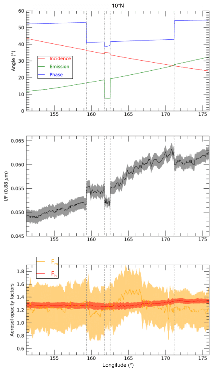
Conclusion
We developed and validated a new RT model for Cassini-VIMS observations of Titan with up-to-date atmospheric optical description. Coupled with an efficient inversion scheme, our model can be apply to the complete VIMS dataset for the retrieval of Titan’s atmospheric opacities and surface albedos at regional and global scales.
References
[1] Rannou, P., McKay, C., & Lorenz, R. 2003, Planetary and Space Science, 51, 963
[2] Karkoschka, E., Schröder, S. E., Tomasko, M. G., & Keller, H. U. 2012, Planetary and Space Science, 60, 342
How to cite: Es-Sayeh, M., Rodriguez, S., Coutelier, M., Rannou, P., Bézard, B., Maltagliati, L., Cornet, T., Grieger, B., Karkoschka, E., Seignovert, B., Le Mouélic, S., Sotin, C., and Coustenis, A.: Updated radiative transfer model for Titan in the near-infrared wavelength range: Validation on Huygens atmospheric and surface measurements and application to the analysis of the VIMS/Cassini observations of the Dragonfly landing area, Europlanet Science Congress 2022, Granada, Spain, 18–23 Sep 2022, EPSC2022-657, https://doi.org/10.5194/epsc2022-657, 2022.
In Titan, the two major gases - dinitrogen (N2) and methane (CH4) are ionized and/or photolyzed at high altitudes by the sunlight and the energetic particles from Saturn's magnetosphere, resulting in rich atmospheric chemistry and a wide variety of carbon and nitrogen-bearing atmospheric compounds. In the present work, we focus on studying the vertical profiles of trace species in the lower atmosphere to obtain a better insight into the atmospheric processes taking place on Titan.
To do so, we reanalyzed the data from the Gas Chromatograph Mass Spectrometer (GCMS) onboard the Huygens probe which executed its mission on 14th January 2005. The GCMS instrument sampled for nearly three and a half hours from an altitude of 146 km. It recorded data for two and a half hours in the atmosphere of Titan, then landed on the surface and kept on recording for another hour, after which the signal was lost. We analyzed the measurements made by direct sampling of the atmosphere (Niemann et al. 2010). These mass spectra obtained at different altitudes and pressure levels have been recalibrated to account for deadtime and saturation corrections to the measurements, set boundary conditions for the species, and considered sensitivity measurements from Cassini-Ion and Neutral Mass Spectrometer calibrations. We then analyzed the corrected mass spectra using Monte-Carlo deconvolution simulations. The simulations allow us to vary the peak intensities of fragmentation patterns of known species, which usually bears uncertainties on this kind of data, and then use a least-square fitting to deconvolve the mixed signals (Gautier et al. 2020, Serigano et al. 2020, 2022).
We present our ongoing effort to retrieve minor compounds' mixing ratios using this approach. As an example, the vertical profile of one of the trace species ethane (C2H6), is shown in figure 1.

Figure 1: Preliminary vertical profile of ethane (C2H6) mixing ratio
In the future, we plan to extend this study to develop a sub-surface model of Titan which will help us understand the outgassing of methane that was observed by the probe upon its touchdown on the surface.
References:
Niemann et al. Composition of Titan’s lower atmosphere and simple surface volatiles as measured by the Cassini-Huygens probe gas chromatograph mass spectrometer experiment. JGR 115, E12006, 2010
Gautier et al. Decomposition of electron ionization mass spectra for space application using a Monte-Carlo approach. Rapid. Com. Mass Spec. 34(8), e8659 (2020)
Serigano et al. Compositional measurements of Saturn’s upper atmosphere and rings from Cassini INMS. JGR:Planets, 125 (8), E006427 (2020)
Serigano et al. Compositional Measurements of Saturn’s Upper Atmosphere and Rings from Cassini INMS: An extended Analysis of Measurements from Cassini’s Grand Finale Orbits. JGR:Planets, 127, E007238 (2022)
How to cite: Das, K., Gautier, T., Serigano, J., Szopa, C., Hörst, S. M., Coutelier, M., Vinatier, S., and Trainer, M. G.: Study of volatile compounds in the atmosphere of Titan, Europlanet Science Congress 2022, Granada, Spain, 18–23 Sep 2022, EPSC2022-710, https://doi.org/10.5194/epsc2022-710, 2022.
The Cassini cameras and especially the Visual and infrared Mapping Spectrometer has provided a sequence of spectra showing the diversity of Titan’s surface spectrum from flybys performed during the 13 years of Cassini’s operation. The investigation of Titan’s surface chemical composition is of great importance for the understanding of the atmosphere-surface-interior system of the moon. The Soi crater region with the well-preserved Soi crater in its center, spans from Titan’s equatorial regions to high northern latitudes. This provides a rich diversity of landscapes, one that is also representative of the diversity encountered across Titan. We mapped this region at 1:800,000 scale using Cassini SAR and non-SAR data and produced a geomorphological map using the methodology presented by [1] and [2]. The VIMS coverage of the region allowed for detailed analysis of spectra of 262 different locations using a radiative transfer technique [3;4] and a mixing model [5;6], yielding compositional constraints on Titan’s optical surface layer. Additional constraints on composition on the near-surface substrate were obtained from microwave emissivity. We identified 22 geomorphological units, 3 of which were not previously described, and derived combinations of top surface materials between dark materials, tholin-like materials, water-ice, and methane. We found no evidence of CO2 and NH3 ice. We also observe empty lakes as far south as 40°N, which mark the most southern extent of Titan’s north polar lakes. We use the stratigraphic relations between our mapping units and the relation between the geomorphology and the composition of the surface layers to build hypotheses on the origin and evolution of the regional geology.
[1] Malaska, M., et al. (2016), Icarus 270, 130; [2] Schoenfeld, A., et al. (2021), Icarus 366, 114516; [3] Solomonidou, A., et al. (2014), J. Geophys. Res. Planets, 119, 1729; [4] Solomonidou, A., et al. (2016), Icarus, 270, 85; [5] Solomonidou, A., et al. (2018), J. Geophys. Res. Planets, 123, 489; [6] Solomonidou, A., et al. (2020), A&A 641, A16.
How to cite: Solomonidou, A., Schoenfeld, A., Malaska, M., lopes, R., Coustenis, A., Birch, S., Le Gall, A., and Schmitt, B.: Chemical composition analysis of Titan’s equatorial and midlatitude surface regions, Europlanet Science Congress 2022, Granada, Spain, 18–23 Sep 2022, EPSC2022-776, https://doi.org/10.5194/epsc2022-776, 2022.
OPS3 | Icy ocean worlds: Past and future explorations
The NASA program exploring habitability places in the outer Solar System searches for simple forms of life in icy moons of Giant Planets, with internal oceans off thermal equilibrium between cold, iced surface and rocky center warmed, possibly by dissipation of tides from the Planet; H2O molecules might lose oxygen to reduced bottom minerals, and get oxygen back when moving upwards. This Ocean World concept was confirmed in Jupiter’s moon Europa, and Saturn’s moons Titan and Enceladus, the last one ejecting a local plume through ice, though not Titan, with the Europa-plume case apparently confirmed. In 2017, H2 molecules, considered sign of life, were detected at the Enceladus plume. We here propose a mission to explore the only large Neptune moon, Triton, which is usually considered an important Kuiper Belt Object as captured dwarf planet. More relevant, here, is that Voyager 2, in 1989, found evidence of Triton ejecting a kind of plume.
Ice Giants, however, have only received flyby missions, at difference with Gas Giants: An effective orbiter-type mission to faraway Neptune is acknowledged as extremely expensive, trip-average solar power is almost nil, chemical capture leads to high wet-mass, with scientific load and orbital maneuvers very constrained. NASA had set a nuclear reactor in space for on-board S/C power in April 1965 but afterwards, for safety considerations, it always used a Radioisotope Pu 238 power system (helpful in mission Cassini). In a sense constraints trade occurred in 2009, between proposed Triton missions a) with full modern technology but just a flyby (EPSC/Potsdam) and b) captured orbiter though with minimum technology (National Research Council / Planetary Science Decadal Survey). Aerocapture and Radioisotope, for propulsion and power, have been considered for Neptune missions, but decayed consideration.
Magnetic Solution to Power and Propulsion Issues
Icy moon missions could use, however, thin, multi-kilometer conductive tethers, with no power or propulsion needs, available to a S/C if passing near the planet. The planetary magnetic dipole allows free –thermodynamically dissipative- S/C capture, and afterwards maneuvering: The relative S/C velocity induces a motional electric field Em (in the tether frame) in the highly conductive plasma around, which polarizes the tether and drives a current I inside, with I ·Em > 0, the field B then exerting Lorentz drag on the current. Driving, however, was ineffective in tethers standard in the 90`s such as TSS1 and TSS1R, insulated all along, with a conductive sphere large enough at the anodic end, typically implying radius much greater than ambient Debye length and thermal electron gyroradius, strongly reducing electron collection. Bare tethers [1] eliminated sphere and insulation to allow electron collection over a resulting anodic tether segment, as a giant cylindrical Langmuir probe, in the optimal OML (orbital-motion-limited) regime. Laframboise and Parker [2] had proved that OML current to cylindrical probes of convex cross-section and equal perimeter p are equal. Thin tape cross-section will reduce tether mass when compared to an equal p tether with round cross-section. Bare tethers, which made standard tethers rapidly obsolete, will thus be characterized by all 3 dimensions, length, width and thickness, widely differing, allowing particular design easier.
Lorentz drag decreasing as the inverse 6th power of radial distance to dipole, capture periapsis would need be very close to the Planet. Keeping current on following capture would hardly affect it, whereas apoapsis could be lowered to finally reach 1:1 Laplace resonance of S/C and moon of interest.
Bare Tether Validation and Use
Bare-tether analysis was validated in early 2001 in an unintended way [3]. Measurements at the International Space Station involving 3 NASA Centers, NOAA/Boulder. Univ-Houston and SAIC, showed on-board plasma-contactors ejecting substantial electron current as if ISS structure had become very negative. Authors acknowledged in the Abstract that tensioning rods of solar array masts could collect ambient electrons as bare-wire tethers, with modeling “based upon J.R. Sanmartin’s bare-wire collection theory’, which was incorporated into the complex ISS computer code, Environment Work Bench, including models of Station, orbital motion, earth’s magnetic field, and ionosphere.
Further, in 2007, Vlasov-code simulations in the high–bias OML regime, at an Unuversity of Michigan PhD Thesis by E. Choinière on the electron density versus radial distance [4] were shown equal to a high approximation when compared [5] with detailed results from the bare-tether theory.
To date, the bare tether analysis has been applied in considering missions to moons Europa [6] and Enceladus [7], and to Ice Planet Neptune [8]}
References
[1] JR Sanmartin, M Martinez-Sanchez, E Ahedo, J. Prop & Power 9, 353-360, 1993
[2] JG Laframboise, LW Parker, Phys. Fluids 16 629-636, 1973
[3] EA Bering et al, Paper 2002-0935, 40th AIAA Aerospace Sciences Meeting and Exhibit, Reno, NV, 14-17 Jan 2002
[4] E Choinière, BE Gilchrist, IEE Trans on Plasma Science 35, 7-22, 2007
[5] JR Sanmartin, E Choinière, BE Gilchrist, J-B Ferry, M Martinez-Sanchez, IEE Trans in Plasma Science 36, 2851-2858, 2008
[6] JR Sanmartin et al, J. Prop & Power 33, 338-342, 2017
[7] JR Sanmartin, J Pelaez, Acta Astronautica 168, 200-203, 2020
[8] JR Sanmartin, J Pelaez, Acta Astronautica 177, 906-911, 2020
How to cite: Sanmartin, J. and Pelaez, J.: Exploring moon Triton, Europlanet Science Congress 2022, Granada, Spain, 18–23 Sep 2022, EPSC2022-39, https://doi.org/10.5194/epsc2022-39, 2022.
To assess the potential habitability of Europa, it is important to understand its chemical composition (Hand et al., 2007). Young terrain features on Europa’s surface likely consist of material up-welled from the liquid water source below (Wilson et al., 1997; Pappalardo et al., 1998; McCord et al., 1999; Figueredo and Greeley, 2004; Mével and Mercier, 2007), encoding relevant compositional information. A major science objective of NASA’s Europa Clipper mission is to characterize the composition of young terrain features using data acquired on close flybys. The Surface Dust Analyzer (SUDA) is an in situ instrument that collects and analyzes the composition of individual grains (Kempf et al., 2012), which are ejected from Europa’s surface by a continuous bombardment of interplanetary impactors (Krüger et al., 1999, 2003; Goode et al., 2021). By applying a dynamical model to these particles, we compute the probability of SUDA’s detections originating from a given feature along the flyby trajectory based on Monte Carlo (MC) simulations. The time-of-flight (TOF) mass spectra that characterizes the chemical composition of individual grains results in a time series of various compositional types along the flyby. We present here a method to analyze a time series of compositional spectra recorded by SUDA that provides a robust estimate for the abundance of different compositional types on the surface, resolved for features along the ground track of the flyby. By demonstrating the association of compositional detections with geological sites of origin, data collected by SUDA is used to infer the compositional ground truth for young terrain features on Europa.
How to cite: Goode, W., Kempf, S., and Schmidt, J.: Mapping the composition of Europa’s young terrain features with SUDA, Europlanet Science Congress 2022, Granada, Spain, 18–23 Sep 2022, EPSC2022-150, https://doi.org/10.5194/epsc2022-150, 2022.
1. Introduction
Liquid water reservoirs in Europa's icy crust, if they exist, could represent the most accessible liquid water bodies in the outer solar system. Previous studies have demonstrated that freezing cryoreservoirs might trigger eruptions due to the pressurization associated with volume change as liquid water expands to become water ice [1, 2]. Locating potentially stored and erupted brines is key for the exploration of ocean worlds and the search for habitability and life beyond Earth.
Here, we aim to numerically model the coupled chemical evolution and pressurization of freezing brines stored in Europa’s ice shell using current best estimates of the oceanic composition [3] to predict the composition of erupted cryolava. This composition varies with time, as salts concentrate during freezing [4], which could lead to erupted brines of varying composition depending on the reservoir frozen fraction when the eruption is triggered. This could explain the variations of albedo observed around features potentially associated with cryovolcanism, for example smooth plains, as shown in Fig. 1.
Figure 1: Smooth plain on Europa’s surface with morphology consistent with eruption of liquid cryolava [1]. The yellow and orange arrow indicate two areas of different albedo, which may have been emplaced by two eruptive events of brines of different composition. NASA Galileo image 9352r.
2. Methods
Cryomagma chemistry Whether they are formed by in-situ melting [5] or intrusion of oceanic water [6], the best estimate for cryomagmatic fluid composition is provided by models of evolution of Europa’s interior and ocean. An example cryomagma composition used in our model, consistent with oceanic compositions predicted by recent literature [3], in wt.%, is 99.0% H2O, 0.32% Na, 0.28% Cl, 0.16% bicarbonate, 0.21% sulfate, 0.027% K, 0.013% Ca, and 0.002% Mg. The equilibrium freezing of oceanic brines is modeled using the software PHREEQC [7] to obtain the liquid and solid fraction of each component of the aqueous solution as a function of the temperature. We use these data as an input of the model presented below.
Model principle Previous studies [1, 2] demonstrated that internal overpressure increases in potential freezing cryoreservoirs as cryomagma transitions to the less-dense solid phase. The critical freezing time required to break the reservoir and trigger an eruption is a function of the reservoir chemical and physical parameters (see example in Fig. 2 for a spherical 500 m radius reservoir located 2 km below the surface and filled with pure liquid water [1, 2]). The cryomagma chemical evolution during freezing will affect the solution and formed ice densities, and can thus make the critical freezing time different from what was calculated by previous studies. We thus need to model the cryomagma composition and internal overpressure as coupled variables. By doing so, we will be able to predict a realistic critical freezing time to trigger eruptions, as well as the
cryomagma composition when the eruption begins.
Figure 2: Pressure as a function of the time in a 500 m radius freezing cryoreservoir located 2 km below the surface. Here the cryomagma is composed of pure water only [2].
Numerical procedure We couple temperature-dependent compositional outputs from PHREEQC with a 1D numerical simulation using the finite differences method to simulate a freezing cryoreservoir. At each time step (i.e., reservoir temperature), we vary the composition of the formed ice and remaining aqueous solution. We modify several parameters accordingly, such as the liquid and solid densities and thermal conductivities. We ensure the energy and mass are conserved through time by calculating the cryomagma frozen fraction that balances the heat lost during each time step. As an output of the model, we can obtain the temporal evolution of: (i) the temperature in the reservoir, (ii) the composition of the formed solid and the remaining liquid and (iii) the internal overpressure. Finally, we can predict the composition of the erupted brines once (and if) the eruption is triggered.
Cyclic eruptions After the first eruption, cryomagma reservoirs may keep freezing and trigger several other eruptions as evoked in Lesage et al. [8]. We added the possibility to continue freezing and trigger several eruptions to our numerical simulation so that we can observe the evolution of erupted brines composition through time.
3. Preliminary results
Initial results demonstrate that salts concentrate in the reservoir during freezing, which decreases the solution freezing temperature and can make the freezing slower than expected with simpler models [1, 2]. On the other hand, the ice formed is initially mostly composed of pure liquid water and thus has a low density compared to the remaining liquid, which can accelerate the pressurization. The effect of both these mechanisms on the critical freezing time have to be quantified. The concentration of non-water components through time is also expected to result in cryolava flows with darker albedo and varying spectral signatures in the case of repeated eruptive events. These results will inform the upcoming missions JUICE (ESA) [9] and Europa Clipper (NASA) [10] on the spectral signatures that could indicate the presence of shallow sub-surface cryoreservoirs and provide information on their activity.
Acknowledgements
Portions of this research were carried out at the Jet Propulsion Laboratory, California Institute of Technology, under contract with the National Aeronautics and Space Administration (NASA). This work was supported by Scientific Exploration Subsurface Access Mechanism for Europa (SESAME) grant number 80NSSC19K0614 and by NASA’s Solar System Workings program (#80NSSC20K0139). The PHREEQC routine is available at https://github.com/MarcNeveu/frezchem.
References
[1] Lesage E. et al. (2020) Icarus, 335, 11336, [2] Lesage E. et al. (2022) The Planetary Science Journal, in press., [3] Melwani Daswani et al. (2021) Geophysical Research Letters, 48(18), [4] Zolotov M. Y. & Kargel J. S. (2009) Tucson, AZ: University of Arizona Press, [5] Kalousová et al. (2016) Journal of Geophysical Research: Planets, 121(12), 2444-2462, [6] Craft K. L. et al. (2016) Icarus, 274, 297-313, [7] Parkhurst, D. L. (1995). User's guide to PHREEQC, [8] Lesage et al. (2021) Icarus, 361, 114373, [9] Grasset O. et al. (2013) Planetary and Space Science, 78, 1-21, [10] Howell S. M. and Pappalardo R. T. (2020) Nature Communications, 11, 1311.
How to cite: Lesage, E., Howell, S. M., Naseem, M., Neveu, M., Melwani Daswani, M., and Vance, S. D.: Chemical composition of erupted brines on Europa, Europlanet Science Congress 2022, Granada, Spain, 18–23 Sep 2022, EPSC2022-301, https://doi.org/10.5194/epsc2022-301, 2022.
Context: Enceladus, an icy moon of Saturn, possesses an internal water ocean and geysers expelling ocean material into space. Cassini investigations indicated the ocean could be habitable and has a complex interaction with the rocky core. Further investigation of the composition of the plume formed by the geysers is necessary to fully understand the ocean, its possible habitability, and what it tells us about Enceladus’ origin.
Mission profile: Moonraker has been proposed as an ESA M-class mission designed to orbit Saturn and perform multiple flybys of Enceladus, focusing on traversals of the plume. Moonraker consists of an ESA-built platform, with strong heritage from JUICE (and Mars Sample Return for solar power), and carrying a suite of instruments dedicated to plume and surface analysis. The nominal Moonraker mission includes a 23-flyby segment, with the possibility of expanding the mission with additional similar segments, depending on available resources.
Objectives and expected impact: Moonraker is devoted to the investigation of i) the habitability conditions of present- day Enceladus and its internal ocean, ii) the mechanisms at play for the communication between the internal ocean and the surface of the South Polar Terrain, and iii) the formation conditions of the moon in the context of the formation of the Saturnian system. Moonraker, thanks to state-of-the-art instruments that represent a vast improvement over Cassini’s payload, would quantify the abundance of key species in the plume, isotopic ratios, and physical parameters of the plume and the surface. Such a mission would allow to solve the standing questions left by Cassini on the aforementioned topics as well as pave the way for a possible future lander mission.
How to cite: Mousis, O., Bouquet, A., Langevin, Y., André, N., Durry, G., Hartogh, P., Helbert, J., Iess, L., Kempf, S., Masters, A., Postberg, F., Renard, J.-B., Vernazza, P., Vorburger, A., and Wurz, P. and the Moonraker team: Moonraker - an Enceladus Multiple Flyby Mission Submitted to the ESA 2021 M-class Call, Europlanet Science Congress 2022, Granada, Spain, 18–23 Sep 2022, EPSC2022-329, https://doi.org/10.5194/epsc2022-329, 2022.
Introduction
Europa's surface is the youngest of the icy satellites and shows signs of recent activity [1]. The main driver of this activity is Jupiter’s tidal forces which are responsible for the existence of a global water ocean underneath Europa’s icy crust [2]. This ocean is thought to be in a direct contact with the rocky mantle [3] creating a potential environment for the emergence of life.
This places Europa at the center of future space exploration with NASA’s Europa Clipper mission [4] as well as ESA’s JUpiter ICy moons Explorer (JUICE) that will more generally study the Jovian icy moons [5].
To prepare for those missions, it is crucial to get the most out of the data we currently have. Photometry plays a key role in deriving remote sensing science products. As such, photometric correction is often the first step of any remote sensing analysis such as mapping or spectroscopy. In itself, photometry is closely linked to the surface microtexture and can help us better understand its physical state [e.g. 6, 7].
In this work, we are deriving photometric parameters for selected areas of Europa - we analyze their spectral dependency and how that can be translated into physical properties.
Dataset
We are revisiting data from Galileo’s Near Infrared Mapping Spectrometer (NIMS) [8] that operated between 0.7 – 5.2 m.
Calibrated and georeferenced data cubes (g-cubes) archived in the PDS Imaging Node have been stored in a database [9] with relevant information such as longitude, latitude, wavelengths, reflectance value, photometric angles etc. This tool allows for a comprehensive view of the dataset and quick exploration to assess the surface and angle coverage available for our study.
Due to changes in the wavelengths calibration and detector failures during operations, the phase angle coverage is very variable across the spectrum (from one cube to the other) with ranges from a few degrees to 80 degrees. We favor spectral intervals with a dense phase coverage. Moreover, to accommodate the shift in the wavelengths reference over time as well as to maximize our geometric diversity, we will not be looking at specific wavelengths but at 40 nm wide ranges of wavelengths across the spectrum.
We retrieved the reflectance and geometry information for a selection of regions of interest across the surface (Figure 1) by finding a compromise between interesting regions and relevant phase angle and spectral coverage.
Figure 1: Map of Europa (credits: Björn Jónsson) with studied areas highlighted
Estimation of photometric parameters
For each area we are considering, we estimated a set of photometric parameters for every 40 nm wavelength interval we have defined. For this work, we are considering Hapke’s direct model detailed in [10] and [11]. Six parameters are to be estimated: phase function (b, c), single-scattering albedo (ω), rugosity (θ ̅), opposition effect (h and B_0).
We used an estimation method based on Bayesian statistics and that we developed for our regional studies of Jupiter’s icy moons in the visible [12, 13, 14]. This allows for of the parameters was inferred except for their physical domain of variation. The posterior Probability Density Functions (PDFs) are sampled with a Monte Carlo Markov Chain algorithm.
Results
We analyzed the different parameters over our three areas of study. Results were very heterogeneous in terms of accuracy across the spectrum but it is clear that the photometric parameters do vary somewhat with the wavelength, as also observed in laboratory experiment [15].
Figure 2 shows the example of the single-scattering albedo and macroscopic roughness estimations between 700 nm and 5 μm for ROI#1 in the leading hemisphere and a sample of wavelengths for which we have well constrained results.
Even though with naïve theoretical considerations we would expect a constant roughness - independent of wavelength - we found here that θ ̅ seems to become more important with higher wavelengths and lower reflectance. This could be related to specific absorption patterns or the presence of certain inclusions that would influence the photometric behavior in preferred wavelengths. In addition, roughness, as observed at various scales determined by the wavelength, may differ in natural material. This phenomenon is known as scale dependence roughness and may play a role here. Here we confirm the first-order dependence of absorptivity and roughness, determined in laboratory measurements [15].
Figure 2: Spectral evolution of the single scattering albedo (left) and the macroscopic roughness (right) for ROI#1 estimated via mean of posterior distribution (blue) and maximum likelihood (orange)
Conclusion and future work
Based on this work, we aim at locally derive photometric corrections that can be used for other remote sensing products like mapping and spectroscopy. The physical implications of a spectrally dependent macroscopic roughness or phase function might also contribute to a better understanding of the history of Europa’s surface and will be our primary focus going forward.
Studying the spectral dependence of the Hapke parameters specifically is interesting as this model is one of the most widely used to investigate radiative transfer in relation to planetary surfaces. Nonetheless, a lot of different photometric models could also be considered. We plan to complement this work by studying the spectral dependency of other photometric models [e.g. 14, 16].
References
[1] Pappalardo, R. T. et al. (1999) JGR: Planets, 104 (E10) :24015_24055. [2] Carr, M. H. et al. (1998) Nature. [3] Vance, S. D. et al. (2018) JGR: Planets, 123. [4] Phillips, C. B. and Pappalardo, R. T. (2014) Eos, Transactions American Geophysical Union. [5] Grasset, O. et al. (2012) Planetary and Space Science. [6] A. McGuire, A. and Hapke, B. (1995) Icarus. [7] Souchon, A. et al. (2011) Icarus. [8] Carlson, R. W. et al (1992) Space Science Review. [9] Cornet, T. et al. EPSC 2022. [10] Hapke, B. (1993) Cambridge University Press. [11] Hapke, B. (2002) Icarus, vol. 157. [12] Schmidt, F. and Bourguignon, S. (2019) Icarus. [13] Belgacem, I. et al. (2019) Icarus. [14] Belgacem, I. et al. (2021) Icarus, vol 369. [15] Pilorget, C. et al., (2016) Icarus [16] Oren, M., Nayar, S. K. (1994) SIGGRAPH94.
How to cite: Belgacem, I., Cornet, T., Schmidt, F., Cruz Mermy, G., Andrieu, F., and Altobelli, N.: Spectral variation of Europa’s regional photometry, Europlanet Science Congress 2022, Granada, Spain, 18–23 Sep 2022, EPSC2022-359, https://doi.org/10.5194/epsc2022-359, 2022.
There is a volatiles enrichment in planetary bodies with the distance from the Sun because the lower temperatures caused their condensation during the solar system formation. As a consequence, the role of volatiles in the geochemistry and thermal evolution became important on certain bodies of the outer solar system, such as the ocean worlds. In order to understand both, physico-chemical interactions between volatiles and salts or other minerals also present in the internal aqueous reservoirs should be characterized. In this regard, the H2O-CO2-Na2CO3-NH3-CH3OH system is a potential candidate to be present within some ocean worlds, such as Enceladus, Titan and Triton. Whereas carbon dioxide (CO2) has been widely detected on icy satellites [e.g., 1-3], signatures of other volatiles such as ammonia (NH3) and methanol (CH3OH) are scarce and have only been found in low concentrations [4], despite their presence is theoretically expected [5-8]. A plausible explanation for the absence of these volatiles on icy moon surfaces is that they reacted at the interior with other substances, forming new compounds [9]. In addition, we included carbonates in our experiments since they are found in carbonaceous chondrites that have suffered low-temperature hydrothermal alteration, and therefore might be considered to come from the outer region of the solar system [10].
In this presentation we will show the results of the Raman spectroscopy kinetic study of the systems H2O-CO2-NH3, H2O-CO2-NH3-CH3OH, H2O-Na2CO3-NH3, and H2O-Na2CO3-NH3-CH3OH, which were exposed to temperatures down to 230 K and pressures up to 50 MPa. From the Raman spectra taken in situ throughout the experiments performed in a high-pressure cell, we were able to monitor the changes in pH of the systems by analyzing the carbonate-bicarbonate ion peak intensity ratio at each time step due to variations in aqueous chemical speciation and precipitation of solids. Our experiments also allowed us to evaluate the active role of CH3OH in the redox equilibria of the systems over time. Finally, the solubility of the carbonates formed was also investigated first, in a CO2 atmosphere, and then at high-pressure water.
This study is the progress of a previous work carried out by differential scanning calorimetry (DSC) [11], where we confirmed that CO2 clathrates stabilize in coexistence with carbonates. In this work, we observed that the presence of salts and volatiles during clathrate formation affect their level of cage occupancy, resulting in less-stable partially-filled structures with low dissociation enthalpies.
This work is funded by the Spanish State Research Agency (AEI) Project No. MDM-2017-0737 Unidad de Excelencia "María de Maeztu"- Centro de Astrobiología (CSIC-INTA). We also acknowledge support from the Spanish MINECO project PID2019-107472RB-C32.
References:
[1] Hansen and McCord. Geophys. Res. Lett. 2008, 35 (1), L01202.
[2] Cruikshank et al. Icarus 2010, 206 (2), 561–572.
[3] Grundy et al. Icarus 2006, 184 (2), 543–555.
[4] Grasset et al. Space Sci. Rev. 2017, 212 (1), 835–875.
[5] Sohl et al. Space Sci. Rev. 2010, 153 (1), 485–510.
[6] Deschamps et al. Astrophys. J. 2010, 724 (2), 887–894.
[7] Dougherty et al. J. Geophys. Res. Planets 2018, 123 (12), 3080–3087.
[8] Tobie et al. Icarus 2005, 175 (2), 496–502.
[9] Kargel. Icarus 1992, 100 (2), 556–574.
[10] Johnson and Prinz. Geochim. Cosmochim. Acta 1993, 57 (12), 2843–2852.
[11] Muñoz-Iglesias and Prieto-Ballesteros. ACS Earth Space Chem. 2021, 5 (10), 2626–2637.
How to cite: Munoz-Iglesias, V., de Dios-Cubillas, A., and Prieto-Ballesteros, O.: Physico-chemical evolution of the H2O-CO2-Na2CO3-NH3-CH3OH system at low temperatures and high pressures. Implications for icy ocean worlds., Europlanet Science Congress 2022, Granada, Spain, 18–23 Sep 2022, EPSC2022-393, https://doi.org/10.5194/epsc2022-393, 2022.
The JUpiter ICy moons Explorer (JUICE), the first large-class of the European Space Agency (ESA), is planned to launch in 2023, and one of its main goals is to make detailed observations of Jupiter’s moon Ganymede. The mission will investigate the past and/or recent cryovolcanic and tectonic activity of the moon and the exchange processes with the subsurface and possibly with the ocean. Recently, the science team defined “potential cryovolcanic regions” as a category of high interest for observation by JUICE (Stephan et al., 2021). For preparation of the scientific return of the mission, it is important to study in detail the regions that are considered to be good candidates for past/present activity. Light material areas on Ganymede imaged by Voyager have been suggested to represent dark terrain resurfaced by cryovolcanic flows (e.g., Parmentier et al., 1982), while the dark terrain’s speculated cryovolcanic origin was later disputed based on higher-resolution images of the Galileo mission. Additional Galileo data showed the significant role of tectonism in the formation of the light material areas, while the role of cryovolcanism remained inconclusive. Currently, small, isolated depressions called ‘paterae’, are the best candidate regions for cryovolcanic activity on Ganymede and suggested to be potential caldera-like cryovolcanic source vents (e.g., Spaun et al., 2001). Their nature has been interpreted as “possible cryovolcanic source vents for extrusion of clean icy material to form light material units” (Collins et al., 2013), and their small size is consistent with a cryovolcanic origin that operates on a local scale. The high-resolution JUICE camera, JANUS, in combination with other remote sensing instruments, is expected to resolve many of the mysteries concerning cryovolcanism on Ganymede and the origin of the moon’s varied geologic features. The “potential cryovolcanic regions” identified by the JUICE team includes 19 out of 30 paterae mapped by Collins et al., (2013) using Voyager and Galileo images. In this study, with the aim to enhance the preparation of the JUICE mission and its science return, we present: a thorough view of all 19 paterae regions; a detailed geomorphological characterization and comparison between the Ganymede paterae with paterae from other planetary bodies; and a spectral assessment using Galileo NIMS data.
How to cite: Solomonidou, A., Malaska, M., Stephan, K., Soderlund, K., Valenti, M., Lucchetti, A., Kalousova, K., and Lopes, R.: Ganymede paterae: a priority target for JUICE, Europlanet Science Congress 2022, Granada, Spain, 18–23 Sep 2022, EPSC2022-423, https://doi.org/10.5194/epsc2022-423, 2022.
1. Introduction
With a launch readiness date of late 2024, NASA’s Europa Clipper will set out on a journey to explore the habitability of Jupiter’s moon Europa. Among others, observations by Europa Clipper’s in-situ instruments will provide an understanding of the satellite’s interior structure and compositional makeup. The variability of Jupiter’s magnetic field at Europa induces electric currents within the moon’s conducting ocean layer, the magnitude of which depends on the ocean’s location, extent, and conductivity. Europa is also embedded in a flow of corotating plasma, which continuously impacts and sputters the surface to produce the moon’s atmosphere. In addition, micrometeorite impacts eject particles of the surface to wrap Europa in a cloud of dust. The neutral atmosphere is readily ionized by energetic particles to produce an ionosphere, which gives rise to current systems electromagnetically connecting Europa to Jupiter. The in-situ instruments comprise the Europa Clipper Magnetometer (ECM), the Plasma Instrument for Magnetic Sounding (PIMS), the SUrface Dust Analyzer (SUDA), and the MAss Spectrometer for Planetary Exploration (MASPEX). We present the highlights of these instruments’ development on their path to delivery to assembly, test, and launch operations (ATLO), which have begun in March 2022.
2. Relevant Investigations
2.1. Europa Clipper Magnetometer
The Europa Clipper Magnetometer (ECM) will measure magnetic fields generated by currents induced in Europa’s subsurface ocean and the electromagnetic coupling of the moon to Jupiter. Jupiter’s tilted dipole magnetic field and Europa’s eccentric orbit expose the moon to time-varying magnetic fields inducing eddy currents in the ocean. By measuring the induced field response at multiple frequencies, the ice shell thickness and the ocean layer thickness and conductivity can be uniquely determined. The ECM consists of three fluxgate sensors mounted on an 8.5-m-long boom and a control electronics hosted in a vault shielding it from radiation damage. The use of three sensors allows for dynamic removal of higher-order spacecraft-generated magnetic fields. The flight-model (FM) sensors (Figure 1) have been delivered to Instrument Integration and Testing, and the instrument is awaiting calibration in the fall of 2022.

Figure 1. ECM FM fluxgate sensor.
2.2. Plasma Instrument for Magnetic Sounding
The Plasma Instrument for Magnetic Sounding (PIMS) will measure ions and electrons in Europa’s ionosphere to quantify magnetic fields associated with electric currents driven by dynamic pressure gradients, which are produced by the interaction of corotating Jovian plasma with Europa and its neutral atmosphere. PIMS will further measure the particle population precipitating onto Europa to model surface sputtering rates and constrain the effects of space weathering. In addition, PIMS will characterize the distribution of electrons carrying field-aligned currents coupling Europa to Jupiter’s ionosphere. The PIMS instrument consists of two sensors each hosting two Faraday cups with a 90° field of view. The instrument measures electrons and ions with energies of up to 2 keV and 7 keV/q, respectively, with an energy resolution of <15% and a temporal resolution of 1−4 s. The instrument, including sensor assemblies (Figure 2), is scheduled for delivery to ATLO in June 2022.

Figure 2. PIMS FM Fully Integrated Sensor Assemblies
2.3. Mass Spectrometer for Planetary Exploration
The MAss Spectrometer for Planetary Exploration (MASPEX) measures trace neutral species to determine the composition of Europa’s atmosphere. The atmosphere is produced by particles sputtering off the surface, is augmented by possible contributions from plumes, and is altered by radiolysis. MASPEX will determine the distribution of major volatiles and key organic compounds with respect to latitude and longitude, altitude, solar local time, and will distinguish endogenic and exogenic sources. MASPEX is a multi-bounce time-of-flight mass spectrometer for species with atomic mass ranging from 2 to 500 u. The instrument’s mass resolution m/Dm of 4275 at mass 50 enables measurement of individual fragment ions generated by electron impact ionization of parent molecule. The FM instrument is presently undergoing testing (Figure 3) and is scheduled for delivery to ATLO in August 2022.
Figure 3. Testing of FM MASPEX instrument.
2.4. Surface Dust Analyzer
The SUrface Dust Analyzer (SUDA) will map the chemical composition of particles ejected from Europa’s surface by hypervelocity impacts of micrometeoroids. The dust particles have a typical size of 0.5−1 μm and exhibit a near isotropic distribution and only weak temporal variations. Small fluctuations are expected from variability of exogenous sources, resulting, e.g., from the orbital motion of sources on Io and the stochastic nature of volcanic activity. SUDA is a time-of-flight mass spectrometer for species with atomic mass ranging of up to 200 u and is capable of detecting up to 40 ejecta per second. Owing to the deterministic nature of the ballistic trajectories of the ejected particles, the composition measurements at spacecraft altitude can be correlated with geologic features on the surface. It has been demonstrated that trace amounts of complex organic species embedded in ice grains with abundances <0.1 ppm can be detected. In addition to micrometeorite ejecta, SUDA will measure the makeup of potential plumes by directly sampling microscopic particles. The FM sensor assembly (Figure 4) will be delivered to ATLO in August 2022 as part of the instrument.

Figure 4. SUDA FM sensor assembly.
3. Mission Concept
The current mission design consists of 49 flybys of Europa executed over a ~3.5 year period while the spacecraft is in orbit about Jupiter. The altitudes of closest approach typically range from 25 km to 100 km. The tour is divided into two principal campaigns, visiting first the anti-Jovian hemisphere followed by observations of the sub-Jovian hemisphere. The flybys occur over a wide range of latitudes and longitudes (Figure 5), and they are widely distributed in true anomaly and solar local time. The tour is thus well suited for characterization of the ice shell and ocean and of the atmosphere and ionosphere created through Europa’s interaction with Jupiter’s magnetosphere.
Figure 5. Planned Europa Clipper close approach ground tracks below 1000 km altitude (black), 400 km (green), 100 km yellow, and 50 km (red).
How to cite: Korth, H., Pappalardo, R., Buratti, B., Kempf, S., Kivelson, M., Burch, J., and Westlake, J.: In-situ Investigations of the Europa Clipper Mission, Europlanet Science Congress 2022, Granada, Spain, 18–23 Sep 2022, EPSC2022-429, https://doi.org/10.5194/epsc2022-429, 2022.
The flyby of Pluto by the New Horizons spacecraft in 2015 revealed stricking features in a nitogen ice filled basin named Sputnik Planitia (SP). On the large (few 10 km) scale, irregular polygons [1] have been interpreted as resulting from solid-state convection [2, 3], with down-welling currents at the polygons’ edges [4]. It was first proposed that convection was driven by heating from below, associated with radioactivity in Pluto’s core but it produces a flow that is opposite to the observations with upwelling currents at polygons’ edges [5] (fig. 1a). At the small scale, we can observe pits that have been explained as produced by sublimation of nitrogen ice. The development of this pattern when getting toward the polygons’ sides has been used to estimate the flow velocity on several polygons, of the order 10 cm yr−1 [4]. We proposed [6] that sublimation is also at the origin of convection by cooling the surface: sublimation consumes latent heat which results in the surface of SP being ∼ 5 K colder than the surroundings [7].
We developed a theory to take into account sublimation in a convection model and showed that it leads to a mixed-type (Robin) thermal boundary condition which, in the case of SP is close to that of a fixed temperature. Starting from a uniform temperature in the ice layer, imposing a colder surface value leads to cooling and convection. With the best estimates of the various parameters for SP, a Rayleigh number of order 1 × 10⁵ can be obtained, justifying the possibility of convection. We used a mantle convection model to explore systematically the effect of surface cooling on convection in a temperature-dependent viscosity solid. Depending on the Rayleigh number and the viscosity contrast, we obtain different regimes (fig. 1b), including one with polygons that match the observations of SP (fig. 1c). The five cases that we obtained in that regime can be used to explore the relationships between observed quantities, like the polygonal sizes, and unconstrained ones, like the thickness of the ice layer or the amplitude of topography [6]. Such large-scale dynamics of a solid state layer driven by climate is unprecedented in the knowledge of planetary bodies but might also operate on other volatile rich moons and TNOs.

Figure 1: Convection pattern for bottom heated convection (a), convection driven by sublima- tion at the surface (c) and regime diagram as function of the Rayleigh number and viscosity contrast (b).
References: 1. White, O. L. et al. Icarus 287 (2017). 2. Trowbridge, A. J., Melosh, H. J., Steckloff, J. K. & Freed, A. M. Nature 534 (2016). 3. McKinnon, W. B. et al. Nature 537 (2016). 4. Buhler, P. B. & Ingersoll, A. P. Icarus 300 (2018). 5. Vilella, K. & Deschamps, F. J. Geophys. Res. 122 (2017). 6. Morison, A., Labrosse, S. & Choblet, G. Sublimation-driven convection in Sputnik Planitia on Pluto. Nature 600 (2021). 7. Gladstone, G. R. et al. Science 351 (2016).
How to cite: Morison, A., Labrosse, A., and Choblet, G.: Sublimation driven convection in Sputnik Planitia on Pluto, Europlanet Science Congress 2022, Granada, Spain, 18–23 Sep 2022, EPSC2022-434, https://doi.org/10.5194/epsc2022-434, 2022.
UP-FRONT SUMMARY
Canonically, researchers explore the outermost viscoelastic shells of the Galilean satellites as the layers primarily responsible for the diurnal dissipation of gravitational potential energy stored within their eccentric orbits around Jupiter. In this study, we find that tidal heating within solid, inner iron cores may be a first-order control on the heat budget of the resonant Galilean satellites.
This has widespread implications for body evolution, sustained geologic activity within the core and rocky mantles of these worlds, episodic resurfacing, magmatism, and their future exploration. Understanding the role of metallic core dissipation is key to understanding the habitability of Europa and Ganymede, the potential for a magma ocean on Io, and the history of Callisto. Future measurements by NASA’s Europa Clipper and ESA’s JUICE spacecraft will help to unravel the contributions of core dissipation to these global heat budgets.
DISSIPATIVE CORE PLAUSIBILITY
Observations of Io indicate a metal-rich core (e.g. Van Hoolst et al., 2020). At Europa, Schubert et al. (2009) infer that a metallic core is both permitted and likely, though a core is not uniquely required (Bills et al., 2009). Ganymede’s intrinsic magnetic field provides strong evidence for a metallic core (Schubert et al., 1996). Callisto, however, is likely only partially differentiated, with a dense rocky/metal core and a lighter silicate mantle (e.g. Bagenal et al., 2007). Figure 1 shows constraints on core state for Europa.
Figure 1: For an example Europa, Bulk density (thick) and Moment of Inertia (thin, dashed) constraints (Casajus et al., 2020). Colors show tidal heat flux at the CMB due to only core dissipation.
On Earth, there is a high plausibility that the solid inner core exhibits viscosities ranging from ~1013–1018 Pa s (Ritterbex and Tsuchiya, 2020), reflecting seismic (1013 Pa s), geodynamic (< 1016 Pa s; Buffett, 1997), and orbital constraints (~1013–1014 Pa s; Koot and Dumberry, 2011).
For the range of iron shear moduli applicable to the Galilean cores (~15–45 GPa; Birch, 1952), the viscosities that maximize dissipation are of the order ~1014–1016 Pa s. Newtonian creep likely dominates at the low pressures of the Galilean satellites cores (Van Orman, 2004), and pure iron viscosities (Birch, 1952) are in the range of 1010–1020 Pa s, depending on temperature and grain size (Figure 2).
Figure 2: Pure iron rheology (Birch, 1952) as a function of temperature and grain size.
We estimate dissipated power from the tidal response of Io, Europa, and Ganymede using a Maxwell rheology (Figure 3). We find that core dissipation at Io and Europa can exceed that of their outer viscoelastic layers. At Ganymede, the heat flux contribution from the iron core is less than the radiogenic contribution. However, concentrated at the core-mantle boundary, the heat flux is likely sufficient to sustain continued or episodic melting of the metallic core.
Figure 3: (Left) contours of surface-averaged tidal heat flux as a function of layer viscosity. For Io, white lines indicate constraints from observed dissipation (Lainey et al., 2009). (Right) Phase lag offset between h2 and k2.
ADDRESSING MYSTERIES / SEARCHING FOR ANSWERS
Io’s Magma Ocean: To match observed dissipation, Io’s average mantle viscosity should be ~1014–1013 Pa s (Segatz et al. 1988). However, these values are many orders of magnitude lower than the lowest inferred for Earth’s partially molten asthenosphere (~1019 Pa s; e.g. Dixon et al., 2004) and cannot support the mantle convection associated with high magma eruption temperatures (Moore et al., 2003). The presence of a pervasive “magma ocean” has been proposed to explain discrepancies (e.g. Khurana et al., 2011).
If Io experiences significant core heating, then a rock viscosity consistent with that of Earth’s mantle (1019 Pa s) and core viscosity of ~1015 Pa s can explain the observed heat flux without requiring a magma ocean or low-viscosity mantle (Figure 3).
Periodic Resurfacing and Dynamos at Europa and Ganymede: Europa’s young surface and Ganymede’s terrain dichotomy reflect episodic resurfacing. While dissipation within ice shell would allow rapid changes within those layers, heat conductively diffuses from the core slowly (~100–101 Gyr). Rapid transport may occur through solid-state mantle convection and/or rock melting and ascent from the CMB (Figure 4). Additionally, core melting causes the tidal response to decouple from the solid body (Henning and Hurford, 2014), decimating dissipation.
The timescales for core melting and freezing, the onset and cessation of thermal convection, and the onset and ascent of melting at depth may compete to create an episodicity in seafloor heat flux, and may modulate the response to episodic changes to the orbital configurations of the satellites. Changes in heat flux may drive resurfacing through induced changes in the ice shell thickness and geodynamic state (Nimmo, 2004), and rotational coupling to the interior.
Callisto’s lack of evidence for resurfacing and sustained (un-forced) orbital eccentricity may reflect the absence of a dissipative iron core, and inefficiency of icy dissipation within the satellite.
Observational Predictions: If core dissipation is meaningful today, it may be observable in the phase lag difference between k2and h2 (Figure 1). In the absence of a phase lag offset, we predict that the present-day core may be partially molten, decoupling it from the solid body and decreasing dissipation, potentially producing an intrinsic magnetic field. If an iron core is responsible for Io’s observed high heat flux, we expect the real part of k2 to reflect a solid body (~0.09) rather than a body with an internal fluid layer (~0.5) per Bierson and Nimmo (2016).
Figure 4: Europa’s (surface-averaged) seafloor heat flux (orange dashed line) responds to periodic changes in core dissipation (solid orange line). CMB temperatures (blue) vary from melting across the critical temperature for mantle convection. Heat transfer occurs through (a) diffusion, and (b) self-consistent melt migration and convection.
ACKNOWLEDGEMENTS
This work was performed at the Jet Propulsion Laboratory, California Institute of Technology, under contract with NASA, and supported through the NASA Habitable Worlds (80NM0018D0004), the Europa Clipper project, and the NASA Postdoctoral Program, administered by Oak Ridge Associated Universities under a contract with NASA (80HQTR21CA005).
How to cite: Howell, S., Vance, S., Bills, B., Melwani Daswani, M., Styczinski, M., and Hay, H.: Powering fire and ice with iron: Strong metallic core dissipation within the Galilean satellites, Europlanet Science Congress 2022, Granada, Spain, 18–23 Sep 2022, EPSC2022-729, https://doi.org/10.5194/epsc2022-729, 2022.
Models for the internal structure of the icy satellites Ganymede and Titan, as derived from the data of the Galileo and Cassini-Huygens space missions, suggest that both moons are differentiated with a hydrosphere of ices and liquid water overlaying an inner rocky core. The presence of significant amounts of Insoluble Organic Matter (IOM) in this silicate layer (in quantities consistent with those found in chondrites) has recently been advanced to properly explain the density and moment of inertia of these moons [1]. Interestingly, laboratory experiments at room pressure have shown that the pyrolysis of IOM (starting from temperatures as low as 500 K) gradually releases volatiles such as H2O, CO/CO2, CH4, H2S, and SO2, with possible N-bearing compounds such as N2, NOx and NH3 [2, 3, 4]. This evolution of the IOM could have a defining impact on the habitability and chemical evolution of icy worlds, including the formation of an atmosphere. However, the effect on these thermal reactions of the high pressures found inside large icy worlds remain largely unknown. The purpose of this study is to analyze the chemical and physical evolution of the IOM under the combined pressure and temperature conditions expected inside Titan and Ganymede (pressures from 0.5 to 7 GPa and temperatures up to 1200 K).

Figure 1: Species produced by IOM dissociation at high pressure and high temperature (blue) compared to those produced by pyrolysis at ambient pressure in Kuga et al. (2014) (green) and Okumura and Mimura (2011) (red).
We conducted anvil cell experiments on mixtures of IOM with water at temperatures up to 773 K and pressure up to 8 GPa. The IOM, with a composition of C100H93N65O61, was synthetized at the Nebulotron (CRPG, France [3]), an ultra-high vacuum chamber using a radiofrequency plasma to ionize a N2-CO gas mixture. Systematic pressure and temperature monitoring, and in situ Raman spectroscopy analyses, were conducted during the experiments to characterize the evolution of the samples. Additional infrared analyses were conducted to compare the initial organic matter (as loaded in the anvil cell) with the residual IOM collected at the end of some of the experiments.
During our high-pressure experiments, elevated temperatures led to the production of C- and N-bearing species, as was reported by others during the pyrolysis of dry IOM at room pressure. Our IOM-water mixtures, however, yielded NH3 (rather than N2) as the main N-bearing molecule. Furthermore, CO2 was never observed in our samples; instead, CO3 (as carbonic acid and/or carbonate ions) was identified as the main C-bearing species alongside CH4 (Figure 1). Overall, the degradation of the IOM at high pressure appears to start at slightly higher temperature, although additional experiments are needed to confirm this result (in particular for the formation of CO3 species). Evidence of the restructuration of the IOM appeared in both Raman and infrared spectroscopy.
Our results support that the thermal dissociation of the IOM inside Titan may have contributed to the formation of its atmosphere [5,6]. These results will also prove useful in assessing the chemical evolution of the hydrosphere of icy worlds, notably regarding the formation of gas hydrates inside their high-pressure ice layers.
Acknowledgements:
This research is founded by CNRS 80 PRIME program. This work also acknowledges the financial support from CNES (Centre National d’Etudes Spatiales, France) in preparation of the ESA JUICE mission.
References:
[1] Néri et al. (2020) A carbonaceous chondrite and cometary origin for icy moons of Jupiter and Saturn. Earth and Planetary Science Letters, 530 :115920.
[2] Okumura and Mimura (2011) Gradual and stepwise pyrolysis of insoluble organic matter from the Murchison meteorite revealing chemical structure and isotopic distribution. Geochimica et Cosmochimica Acta, 75(22) :7063–7080.
[3] Kuga et al. (2014) Nitrogen isotopic fractionation during abiotic synthesis of organic solid particles. Earth and Planetary Science Letters, 393:2–13.
[4] Franklin (1949) A study of the fine structure of carbonaceous solids by measurements of true and apparent densities. Part I. Coals. Transactions of the Faraday society, 45:274–286.
[5] Tobie et al. (2012) Titan’s bulk composition constrained by Cassini-Huygens: implication for internal outgassing. The Astrophysical Journal, 752(2):125.
[6] Miller et al. (2019) Contributions from accreted organics to Titan’s atmosphere: new insights from cometary and chondritic data. The Astrophysical Journal, 871(1):59.
How to cite: Lévêque, P., Sotin, C., Bujoli, B., Bollengier, O., Queffelec, C., Le Menn, E., Clouet, A., Marrocchi, Y., and Tobie, G.: Evolution of Insoluble Organic Matter and H2O mixtures Under Ganymede and Titan’s Interior Conditions, Europlanet Science Congress 2022, Granada, Spain, 18–23 Sep 2022, EPSC2022-792, https://doi.org/10.5194/epsc2022-792, 2022.
Galileo Regio is a dark terrain of Ganymede extending approximately from 180°-120° W to 0°-60° N that shows high crater density and morphotectonic structures called furrows. Such structures are kilometric-scale brittle troughs bounded by high albedo rims and a low albedo floor, and arranged with circumferential and radial setting at the regional scale [1]. Furrows are generally interpreted as the remnants of a multi-ring impact basin similar to the Valhalla basin on Callisto [2]. Galileo Regio shows two main settings of the furrows, which allow their classification into two systems: the concentric furrows of Lakhmu Fossae system, which is crosscut by the radial furrows of the Zu Fossae system [3]. In addition, Galileo Regio shows local-scale structures that rework the pristine morphology of the Lakhmu Fossae furrows.
In this contribution, we investigate the furrows of Galileo Regio at both regional- and local-scale to unravel the tectonic evolution of the dark terrain. We perform a structural mapping and geostatistical analyses of the furrows in Galileo Regio, identifying their hierarchy and tectonic setting originated by regional-scale kinematics. Structure attributes such as structure length, sinuosity, azimuth, spacing within the adjacent structures, have been quantitatively characterized and allow to perform the azimuthal distribution, the Length/Spacing [5] and the paleo-stress analyses [6]. Such analyses allow to identify the structural systems and to infer the past stress fields that affected Galileo Regio (maximum and minimum horizontal stress, i.e., SHmax and Shmin, respectively). A total of four structural systems have been recognized within Galileo Regio: i) the already known Lakhmu and Zu Fossae; and ii) the Lineated system and Precursor system, proposed by this work for the first time (Fig. 1).
Such systems are the result of phases of the tectonic activity that affected Galileo Regio during the geologic history of Ganymede. We identify the sequence of such phases that allow to produce an evolutionary tectonic model (Fig. 2): i) t0 represents a NW-SE extension that formed the Lineated system; ii) t1 represents the impact that originated a multi-ring basin [3, 7], i.e., the Lakhmu Fossae; iii) t2 shows the extensional activity responsible for the formation of the light terrain of Uruk Sulcus [8] and for the formation of the extensional structures of the Precursor system; iv) t3 represents the kinematics consistent with the right-lateral transpression that has affected Uruk Sulcus [4] and formed the Zu Fossae; and v) t4 presents a right-lateral strike-slip that contributes to the formation of the Precursor system.
The obtained results and the presented model will be used for the scientific preparation of dedicated high-resolution observations that will be taken with the JANUS instrument [9] onboard the JUICE mission [10].
Acknowledgments: The activity has been realized under the ASI-INAF contract 2018-25-HH.0.
References:
[1] Patterson, W. et al. (2010). Icarus 207,845–867; [2] McKinnon, W.B. and Melosh, H.J. (1980). Icarus 44 (2), 454–471; [3] Prockter, L.M., et al. (2000). Journal of Geophysical Research: Planets, 105(E9), 22519-22540; [4] Kersten, E., et al. (2021). Planetary and Space Science, 206, 105310; [5] Rossi, C., et al. (2018). Tectonophysics 749, 72–87; [5] Delvaux, D., and Sperner, B. (2003). Geol. Soc., London, Special Publications, 212(1), 75-100; [7] Hirata, N., et al. (2020). Icarus, 352, 113941; [8] Pappalardo, R.T., et al. (1998). Icarus, 135(1), 276-302; [9] Palumbo, P., et al. (2014). 45th LPSC Meeting. Abstract #2094; [10] Grasset, O., et al. (2013). Planetary and Space Science, 78, 1–21.
How to cite: Rossi, C., Lucchetti, A., Massironi, M., Pozzobon, R., Penasa, L., Munaretto, G., and Pajola, M.: Structural evolution of Galileo Regio, dark terrain of Ganymede., Europlanet Science Congress 2022, Granada, Spain, 18–23 Sep 2022, EPSC2022-815, https://doi.org/10.5194/epsc2022-815, 2022.
Introduction : Europa’s surface is one of the youngest surfaces in the solar system. The great diversity of morphologies observed quickly raised the question of the processes responsible for this active resurfacing. The Jovian moon is believed to hide a global liquid water ocean under its ice crust [1] which led to the assumptions of exchange between the surface and the putative subsurface ocean [1]. In addition, Europa is exposed to intense space weathering due to the continuous bombardment by electrons and ions from Jupiter’s magnetosphere [2]. The surface therefore appears as the key witness of these internal and external processes.
To finely characterize the microphysics of the ice it is necessary to use radiative transfer (RT) modeling. Such modeling allows to estimate these parameters integrating the highly nonlinear effects of the light path within the icy regolith due to scattering. A recent work has been proposed to determine surface properties using Bayesian Monte Carlo Markov Chain (MCMC) [3]. This approach is based on RT models [4,5] using the optical properties of the considered chemical species and physical properties of the regolith. Here we report the use of a RT model [5] in a Bayesian MCMC inference framework to retrieve microphysical properties of Europa's surface using the Galileo Near-Infrared Mapping Spectrometer (NIMS) hyperspectral data [6].
Data: We use data acquired by NIMS collected during the Galileo mission. Here we present the analysis of calibrated data from the hyperspectral cube "e6007ci" (available from the PDS archive) from the trailing Anti-jovian hemisphere (Fig. 1). The estimated signal-to-noise ratio (SNR) is between 5 and 50, we mainly focus on the 1.0-2.5 µm region for which the SNR is higher. Within this spectral range the uncertainty on the absolute calibration is up to 10% [7].
Radiative transfer model requires the optical constants of the pure chemical species considered. Here we consider 15 different compounds: crystalline and amorphous water ice [7,8], sulfuric acid octahydrate (SAO; [2]), hydrated sulfates [9,10], hydrated chlorine salts [11], and minerals such as magnetite [12], sodium chloride [13] and ammonium sulfate [14].
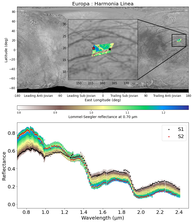
Figure 1 - (top): Map of Europa with a zoom on Harmonia Linea observation. The color represents the reflectance at 0.7 µm normalized using the Lommel-Seegler law. (bottom): all spectra from the corresponding cube and the selected spectra (S1 and S2) used in this study.
Method: We use a MCMC Bayesian inference approach [15,16] to analyze NIMS spectra because it has the advantage of allowing the exploration of a large parameter space and looking for non-unique solutions while statistically constraining the model parameters [17,18]. We compute the bidirectional reflectance of the regolith using a RT model [5]. Then, the algorithm is used to sample the parameter space following the Bayesian Posterior distribution. The parameters we are adjusting are: abundances, grain size of each chemical species and macroscopic roughness of the regolith. For the abundances we use a Dirichlet prior to ensure that they are sum up to 1, while we use a uniform distribution prior for the other parameters.
A first study was done to test all combination of 3, 4 and 5 chemical species among the 15 compounds on the S1 spectrum to select the most appropriate chemical species to consider for the surface characterization. For each of this combination (4823 in total), we perform the MCMC inversion.
Results: We first discuss the chemical species selection (called here endmember) by looking at all best-fit from all combination of 3, 4 and 5 endmembers and their associated RMS. We first show that going from 3 to 4 endmembers significantly improves the quality of the fit while using 5 endmembers only slightly improve it. In addition, some compounds appear necessary to reproduce the observation, such as water ice and SAO. We show that adding either hydrated sulfates or chlorine salts produces results substantially similar. Fig. 2 illustrates such results when considering 4 endmembers. Finally we perform MCMC inversion with 5 endmembers including both crystalline and amorphous water ice. The best fit from the 5 endmembers model and their associated posterior pairwise distribution are shown fig. 3 and 4 for the S1 and S2 spectra.
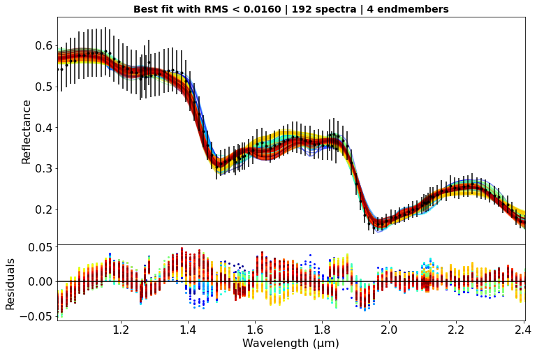
Figure 2 - Results of all combination for the 4 endmembers case: only the best-fit with RMS below 0.016 are showed.
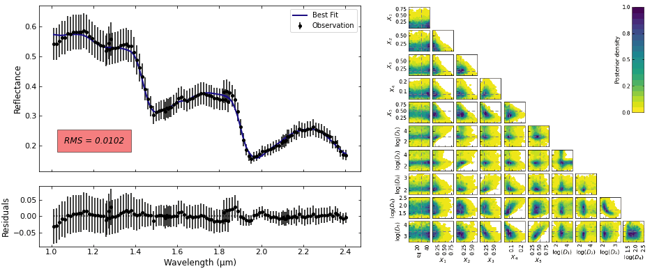
Figure 3 - results for S1: best fit (left) and pairwise posterior distribution (right) using 5 endmembers.
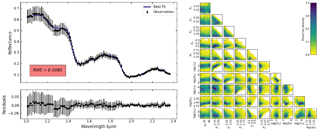
Figure 4 - results for S2: best fit (left) and pairwise posterior distribution (right) using 5 endmembers.
Conclusion: We tested, for the first time and in a systematic way, the inversion of Galileo NIMS infrared spectra using a significant number of 3, 4 and 5 compounds combinations out of a selection of 15 chemical compounds, using a non-linear radiative transfer model. We found that there is no unique solution to determine the exact composition of the surface, but a family of endmember are required: water ice, SAO and sulfates. This composition set seems to be coherent for both bright and dark regions of Europa. We will discuss the implication of these results on the Europa’s surface processes.
References: [1] Pappalardo, R. et al. (1999) JGR. [2] Carlson, R. W. et al. (2005) Icar. [3] Mishra, I. et al. (2021) Planet. Sci. [4] Hapke, B. (2012). Cambridge Univ. Press. [5] Douté. S. and Schmitt. B. (1998) JGR. [6] Carlson, R. et al. (1992) ed. C. T. Russell. [7] Schmitt, B. et al. (2004). [8] Trotta, F and Schmitt, B (2018). [9] Dalton, J.B. et al. (2012) JGRE. [10] D. Angelis, S et al. (2021) Icar.. [11] Hanley, J. et al. (2014), JGR. [12] Roush, T. et al. (2021) Icar. [13] Querry, M. (1987). [14] Fastelli, M. et al. (2022), Icar. [15] Cubillos, P. et al. (2016), The Astr. Jour. [16] Braak, C. J. F. (2008), Stat & Comp. [17] Mosegaard, K. et al. (1995) JGR. [18] Schmidt, F. and Bourguignon, S. (2019) Icar.
How to cite: Cruz Mermy, G., Schmidt, F., Andrieu, F., Belgacem, I., Cornet, T., and Altobelli, N.: New insights into Europa's surface using Galileo/NIMS data and MCMC modeling, Europlanet Science Congress 2022, Granada, Spain, 18–23 Sep 2022, EPSC2022-825, https://doi.org/10.5194/epsc2022-825, 2022.
Events which deposit fresh material onto Europa’s surface may be irregular and catastrophic, such as large-scale impacts, or localized, and potentially extant, processes in which faults, fractures, or brine transport bring subsurface liquid onto the surface. This liquid may originate from shallow reservoirs within the ice shell or directly from the subsurface ocean [1]. Emplacement may be a slow, extrusive process, or quicker, potentially with the formation of cryovolcanic plumes (e.g. [2,3,4]). Plume deposits or any other surface material can also be transported to high altitudes by another mechanism: when hypervelocity interplanetary micrometeoroids, or larger objects, impact the surface of an atmosphereless planetary body like Europa, these can generate impact ejecta with high enough velocities to reach altitudes of hundreds of kilometres [5]. Most of these ejecta particles are gravitationally bound, moving on ballistic trajectories lasting up to hundreds of seconds and producing an almost isotropic dust exosphere around Europa [6,7]. Subsurface oceans, in the Jovian and in other planetary systems, can therefore be characterized using the particles they emit, via either indirect or direct routes: 1) Detection and analysis of ejecta particles lofted by micrometeoroid impacts from those parts of the surface that recently interacted with subsurface water (e.g. certain landforms, such as chaos terrains on Europa, or plume deposits); 2) Direct sampling of plume particles in space (where plumes are present, as perhaps possible on Europa).
The SUrface Dust Analyzer (SUDA), onboard the Europa Clipper spacecraft, is designed to measure the composition and trajectories of such impact ejecta particles and/or plume material. SUDA is an impact ionisation time-of-flight mass spectrometer, which uses the ions generated by hypervelocity impacts of dust grains onto the instrument target to generate mass spectra of the impinging particles. Depending on the altitude, SUDA will be able to detect up to tens of ejected surface particles per second during each flyby, each likely to contain a wide variety of organic and/or inorganic compounds, and via trajectory reconstruction, map them to their origins on the surface [8].
At global scales, landform evolution on atmosphereless bodies is primarily driven by impact gardening and tectonics. The tectonic regime that dominates within Europa’s ice shell is likely to be extensional, a hypothesis supported by numerous lines of evidence, such as the widespread presence of dilational bands that represent >40% of the total surface area [9]. Several types of geological features generated within such a tectonic regime, including chaos terrains and fossae, might affect the emplacement of buried material and subsequent exposure of fresh volatiles on Europa’s surface.
Chaos Terrains are, on Europa, geologically very young and extensively disrupted surface features, interpreted as reflecting recent interaction with subsurface material [10]. Leading-hemisphere chaos regions have recently been shown to be compositionally distinct from their surroundings, probably indicating contributions from endogenous sodium chloride sourced from the subsurface ocean [11,12]. Fossae are long, narrow depressions (troughs). The term is used for topographic features that occur on extraterrestrial planetary surfaces, whose exact origin is uncertain, although they are thought to be the result of extensional tectonic processes [13].
Here we investigate two neighboring features on Europa, Ménec Fossae and Thrace Macula (a chaos terrain), for which we produced high-resolution photoclinometrically-derived [14] digital terrain models (DTMs, Fig. 1) and geomorphological-structural maps (Fig. 2). Our preliminary results suggest that this area of Europa has undergone transtensional (strike-slip paired with extension) tectonic activity, as indicated by the orientation and relationship of the faults and fossae. Such tectonic style has possibly created a pathway facilitating the ascent of subsurface material, especially volatiles, that play an important role in the formation of chaos terrain. These results will help ascertain the most likely regions on Europa in which to find fresh material, representative of the subsurface ocean, and be used as input data for dust ejecta trajectory models that will ultimately assist the mass spectrometer Surface Dust Analyzer (SUDA), onboard the upcoming Europa Clipper mission, in compositionally mapping Europa’s surface [15].
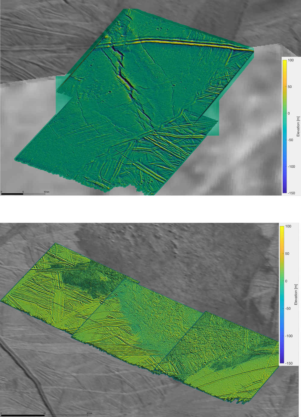
Figure 1. Regional DTMs, Ménec Fossae (top) and Thrace Macula (bottom)
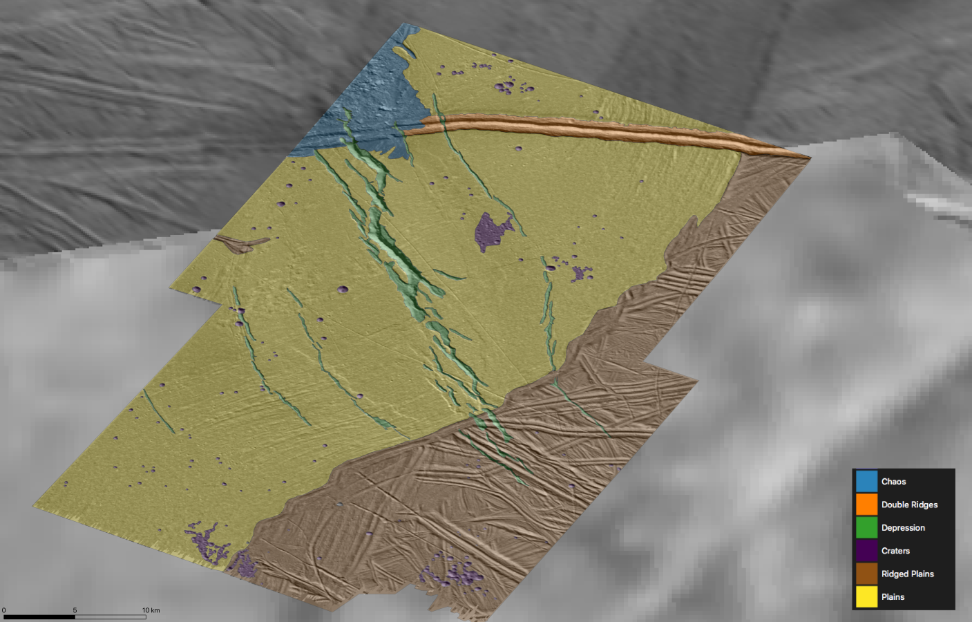
Figure 2. Geomorphological map of Ménec Fossae
- 1. Head, J.W., & Pappalardo, R.T., (1999). J. Geophys. Res. 104, 27143–27155.
- 2. Roth, L., et al., (2014). Science 343, 171.
- 3. Sparks, W.B., et al., (2017). The Astrophysical Journal Letters, 839(2), L18.
- 4. Jia, X., et al., (2018). Nat. Astron. 2, 459.
- 5. Koschny, D., & Grün, E., (2001). Icarus, 154(2), 402-411.
- 6. Krivov, A. V., et al., (2003a). Planetary and Space Science 51, 251-269.
- 7. Postberg, F., et al., (2011). Planetary and Space Science, 59(14), 1815–1825.
- 8. Goode, W., et al., (2021). Planetary and Space Science, 208, 105343
- 9. Kattenhorn, S.A. & Hurford, T.A., (2009). In: Europa, 199-236.
- 10. Schmidt, B. E., et al., (2011). Nature 502, v. 479
- 11. Trumbo, S. K., et al., (2019). SciA, 5, aaw7123
- 12. Trumbo, S. K., et al., (2022), PSJ, 3, 27
- 13. Schenk, P., et al., (2020). Geophys. Res. Let., 47, e2020GL088364
- 14. Lesage et al., (2021). Icarus, Volume 361, 114373.
- 15. Kempf, S., et al., (2019). AGU Fall Meeting 2019, abstract #P53D-3500
How to cite: Matteoni, P., Neesemann, A., Schmidt, J., Hillier, J., and Postberg, F.: Geomorphology and topography of Ménec Fossae and Thrace Macula on Europa: Insights on formation processes, Europlanet Science Congress 2022, Granada, Spain, 18–23 Sep 2022, EPSC2022-914, https://doi.org/10.5194/epsc2022-914, 2022.
Introduction
Tidal dissipation is an important source of heat for several icy moons of Jupiter and Saturn. While the evaluation of tidal heating in the solid parts of the moons is straightforward, with the only limitation being the lack of knowledge about anelastic properties of ice and silicates, modeling the tidal dissipation in subsurface oceans is challenging and the issue of how much it contributes to the total heat production has not yet been fully resolved. The standard approach to modeling the tidal dissipation in a subsurface ocean is based on the solution of hydrodynamic equations in the shallow water approximation [e.g., 1– 4]. Numerical studies addressing the tidal deformation of the ocean in a three-dimensional geometry have appeared only recently [5,6]. Although these studies represent significant progress, they have one important limitation: they do not take into account the mechanical coupling between the flow in the ocean and the viscoelastic deformation of the ice shell and the core. To overcome this limitation, we have developed a new method that allows the tidal deformation to be solved simultaneously in all three parts of the icy moon.
Method
The problem of tidal deformation is solved in a spherical computational domain corresponding in size to Saturn’s moon Enceladus and consisting of three sub-domains (the viscoelastic ice shell, the viscous ocean, and the viscoelastic core), which are coupled by the boundary conditions. The Navier-Stokes equation is integrated in time and solved using a pseudo-spectral method based on spectral decomposition in angular coordinates and finite differences in radius. The spherical harmonic coefficients are discretized in 800 unevenly spaced grid points guaranteeing a sufficiently high sampling density in the boundary layers. Self-gravitation and the Coriolis force are included. The thickness of the ocean is varied from 10 m to about 50 km and its viscosity is considered in the range 1–106 Pa s. Calculations are performed for two end-member cases, recently discussed in literature: a weakly deformable elastic core and a highly deformable Maxwell viscoelastic core [7].
Results and Conclusion
Our results confirm the conclusions of previous studies that tidal dissipation in the present day ocean on Enceladus is negligible compared to the expected heat production [e.g., 8]. However, unlike some previous models, we find less pronounced resonance peaks, suggesting that the mechanical coupling between the ocean and the solid parts of the moon tends to reduce the resonance effects. Our results indicate that dissipation in the ocean strongly depends on the ocean thickness, reaching the maximum value for a thickness of 1 km when the ocean viscosity is 106 Pa s and less than 0.1 km when the viscosity is smaller 10 Pa s. The maximum dissipation predicted in the ocean (1 GW for the weakly deformable core and 20 GW for the highly deformable core) is independent of the viscosity prescribed in the ocean. This suggests that although the tidal dissipation currently plays a negligible role in Enceladus’ heat budget, it can effectively hinder the freezing of the ocean when the ocean is thin.
References
[1] Tyler, 2011, Icarus 211, 770–779.
[2] Chen et al., 2014, Icarus 229, 11-30.
[3] Matsuyama, 2014, Icarus 242, 11–18.
[4] Hay and Matsuyama, 2019, Icarus 319, 68–85.
[5] Rovira-Navarro et al., 2019, Icarus 321, 126–140.
[6] Rekier et al., 2019, J. Geophys. Res.: Planets 124, 2198–2212.
[7] Choblet et al., Nat. Astr. 1, 841–847.
[8] Čadek et al., Icarus 319, 476–484.
How to cite: Aygün, B. and Čadek, O.: A new approach to modeling the tidal dissipation in subsurface oceans of icy moons of Jupiter and Saturn, Europlanet Science Congress 2022, Granada, Spain, 18–23 Sep 2022, EPSC2022-968, https://doi.org/10.5194/epsc2022-968, 2022.
Introduction
The formation of Ganymede’s light terrain and its possible interaction with a subsurface ocean, have made its investigation one of the top goals of the upcoming JUICE mission [1, 2]. In this study we present a detailed stratigraphic analysis of areas that were observed by the Galileo SSI camera at highest possible spatial resolution (scales of ~11 m/pxl) in order to see what information of the light terrain’s stratigraphic position in Ganymede’s surface evolution can be gained from mapping and crater counting results and to identify what still has to be done in order to prepare for the upcoming JUICE mission.
Study areas
Based on the available data set, we selected four major regions (Region A, B, C and D) that are covered by more than one high-resolution SSI image for our study (Fig. 1): Region A and D from the anti-Jovian hemisphere and Region B and C from sub-Jovian hemisphere. Region A comprises of Byblus Sulcus (G2GSGRVLNS01), Nippur and Philus Sulcus (G2GSNIPPUR01) and the Transitional region (G2GSTRANST01) with the context info provided by the SSI observation G8GSREGCON01. Region B is dominated by Arbela Sulcus (28GSARBELA01+02/ G7GSNICHOL01), Region C is the Harpagia Sulcus region (28GSBRTDRK02, 28GSCALDRA02 and 28GSSMOOTH02) and Region D comprises Erech Sulcus (G8GSERECH01), Mummu and Sippar Sulci (G8GSCALDRA01).
Mapping results
Geologic maps are prepared for the four regions using ArcGIS. The naming/categorization of geological units follows from [4, 5] but are refined and modified wherever necessary (Fig. 2). Among the light terrain units, ls and lg are the most commonly occurring than li.
Stratigraphic correlation:
On the whole, the relative ages from crater density measurements (Fig. 5) follow the mapping results. In brief, in Byblus Sulcus the two light terrain units are of similar age from crater counts while lg3 is younger than lg2 from crosscutting relationships. (Fig. 2). In case of Region B (Arbela Sulcus), we could find that the age relationship of the two light terrain units and two dark terrain units agree with the relative age inferred from crosscutting relationship (Fig. 3a) In more extensively resurfaced areas of the light terrain the situation appears to be more complex. In Region C, the terrain units ls also have comparatively higher age than lg terrain units (Fig. 3b-3d). In Region D the terrain units (Fig. 4) are highly interrupted by the secondary craters formed during the Osiris and Melkart impact events [6].
Discussion
We used two most favored chronology models LDM (Lunar Derived Model by [7]) and JCM (Jupiter Comets Model by [8]) (Fig.6). In general, based on the LDM ages the crater densities point to a relatively high age of the light terrain units not much younger that the ancient dark terrain and could imply a relatively short time period of formation for most of our mapped light terrain units. This relatively high age fits into the theory that the light terrain could have formed as a direct result of internal differentiation followed by a global expansion [9]. On the contrary, the JCM derived ages point to a longer formation period of light terrain units around 2 Ga [9]. While the impact chronology in the Jovian system and of its satellites is still not fully solved, newest results infer that the craters on these bodies were created from members of a collisionally evolved impactor family, similar to those in the inner solar system [10]. This does not straightforwardly support the lunar-derived chronology model (LDM) by [7] but allows to derive a Ganymede-specific crater production function empirically from the lunar one. We used this production function to fit our crater distributions and to derive absolute model ages for both model chronologies [7][8].
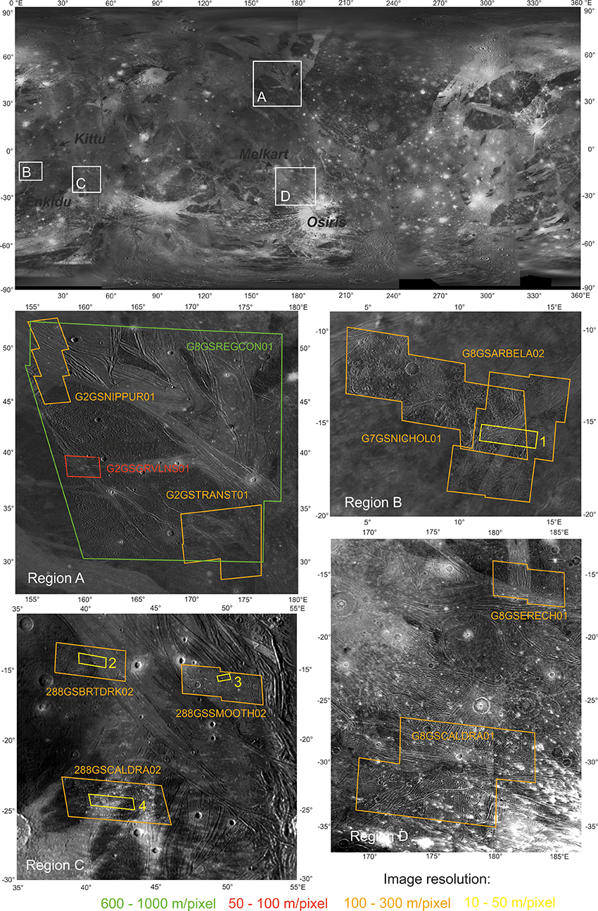
Figure 1: Regions of Interest in this study with the available Galileo SSI coverage indicated.
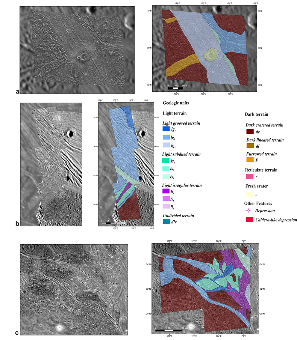
Figure 2: Geologic mapping results for Region A: a) Byblus Sulcus (G2GSGRVLNS01), b) Nippur and Philus Sulcus (G2GSNIPPUR01) and c) the Transitional region (G2TRANST01). The legend applies also to Figures 3 and 4.
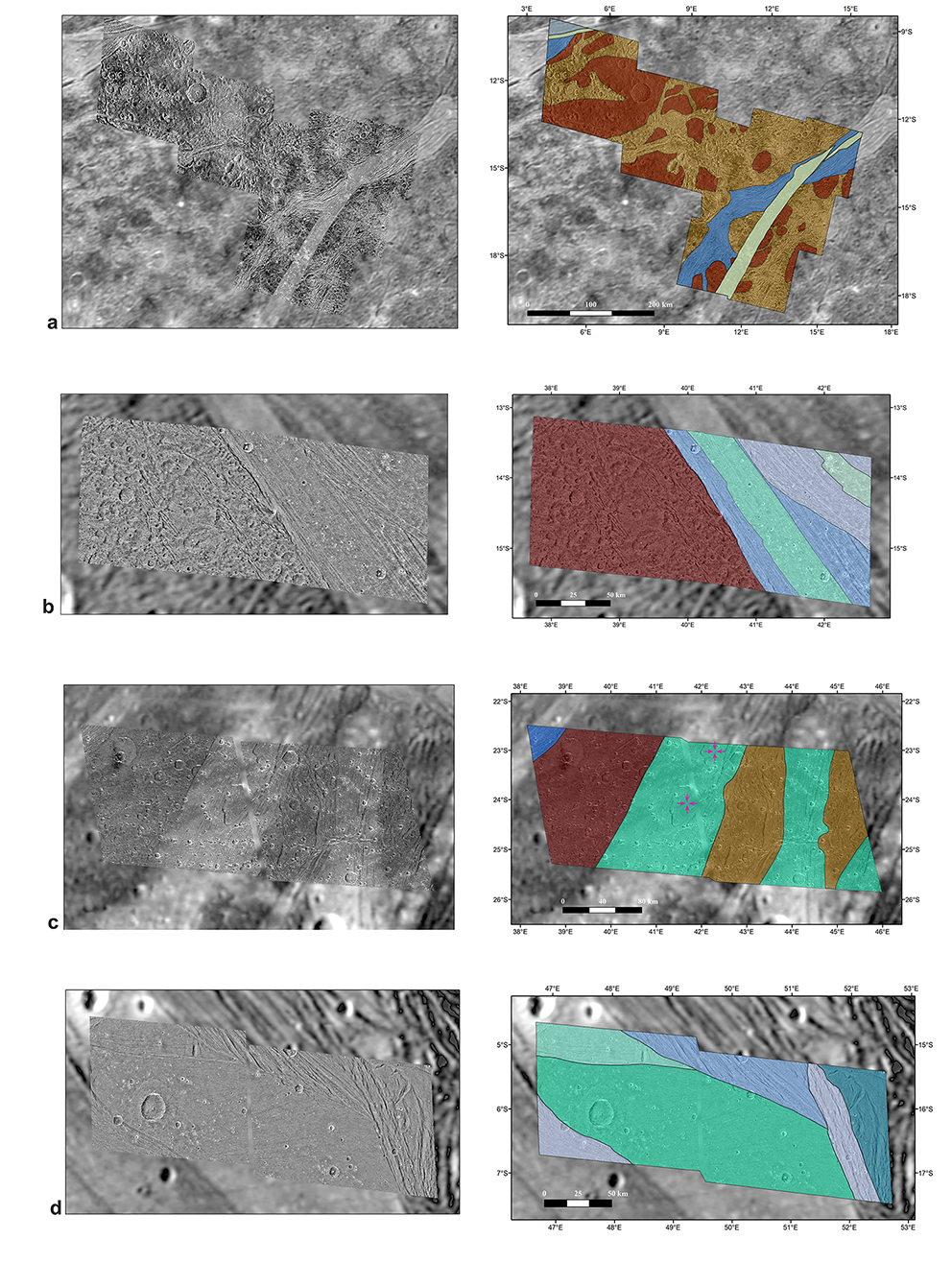
Figure 3: Geologic mapping results for Region B dominated by Arbela Sulcus (28GSARBELA01+02/ G7GSNICHOL01) and Region C by Harpagia Sulcus (b) 28GSBRTDRK02, c) 28GSCALDRA02 and d) 28GSSMOOTH02).
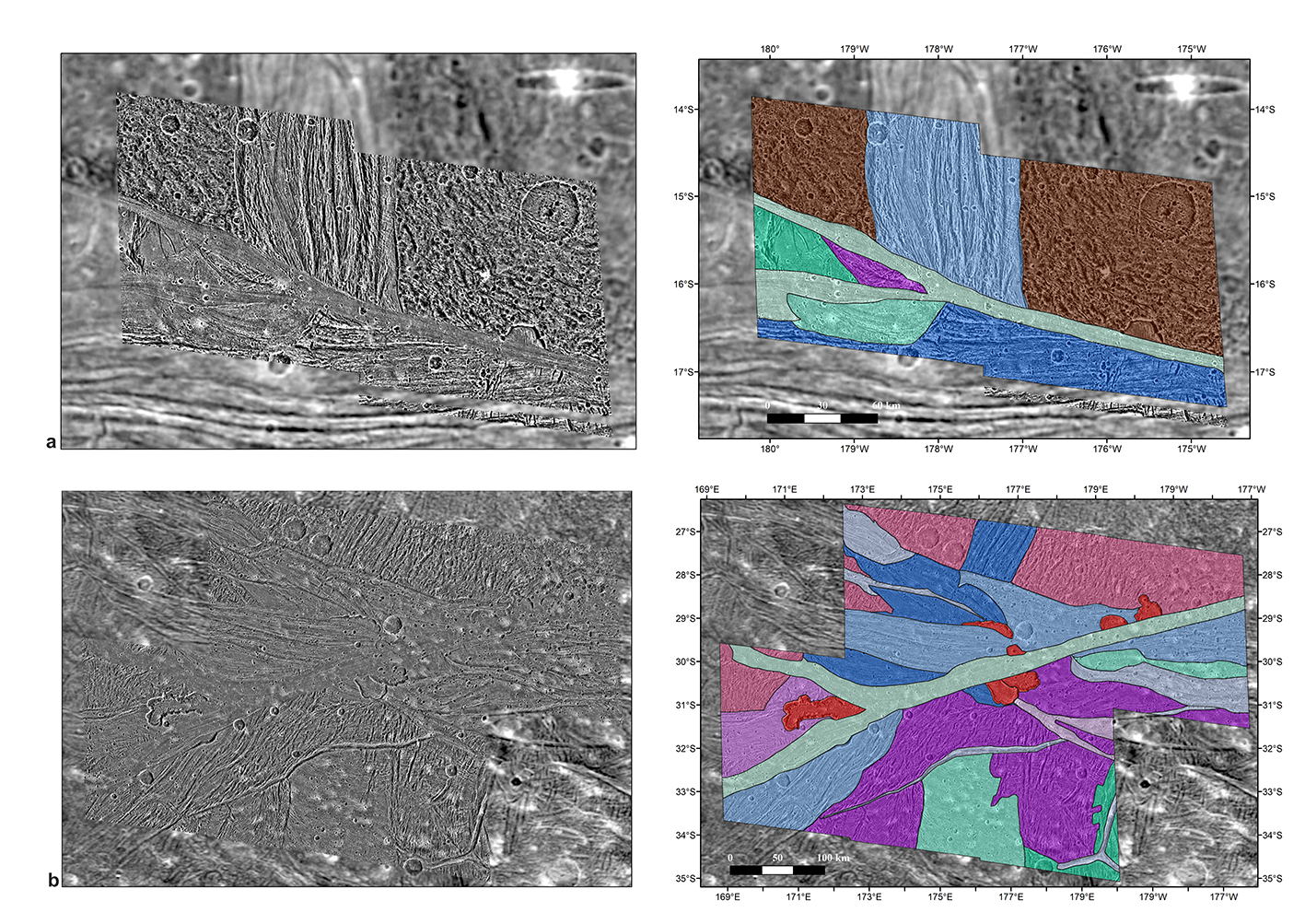
Figure 4: Geologic mapping results for Region D comprises of a) Erech (G8GSERECH01) and b) Mummu and Sippar Sulci (G8GSCALDRA01).
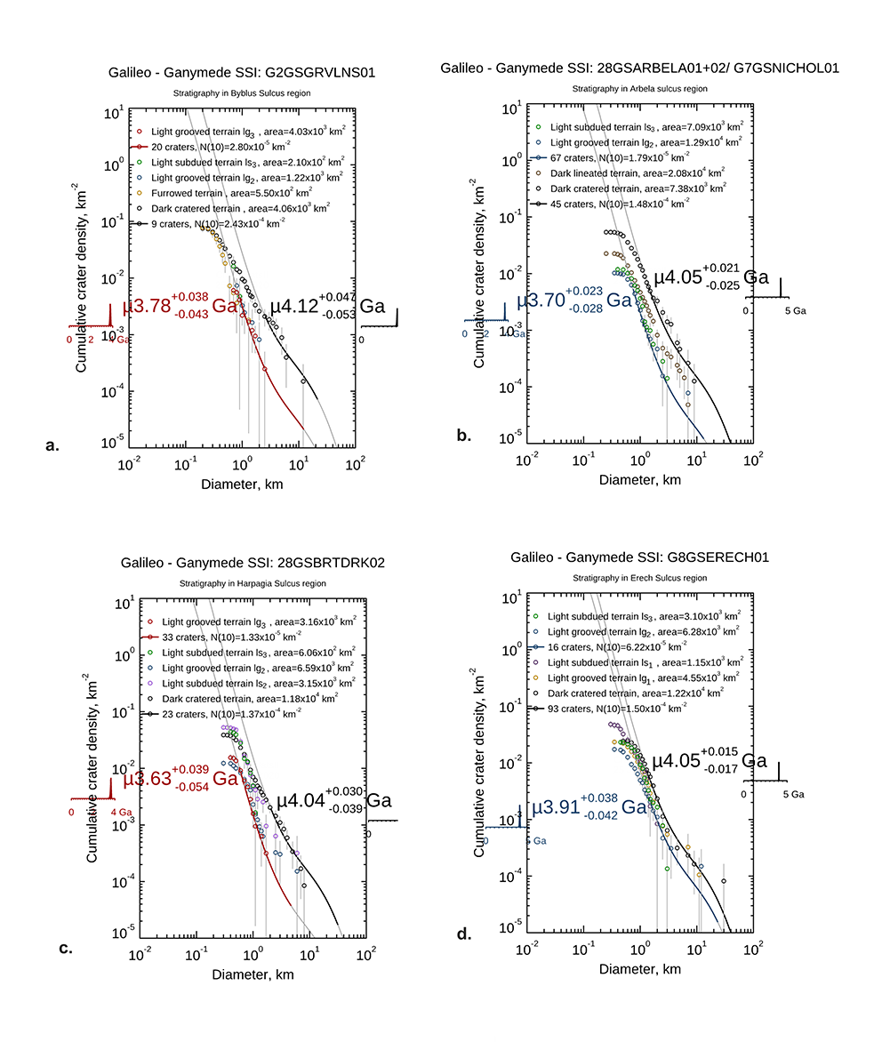
Figure 5: Comparison of relative ages of different terrain units from a) Region A (Byblus Sulcus), b) Region B (Arbela Sulcus), c) Region C (Harpagia Sulcus - 28GSBRTDRK02) and d) Region D (Erech Sulcus) based on crater size frequency distributions.
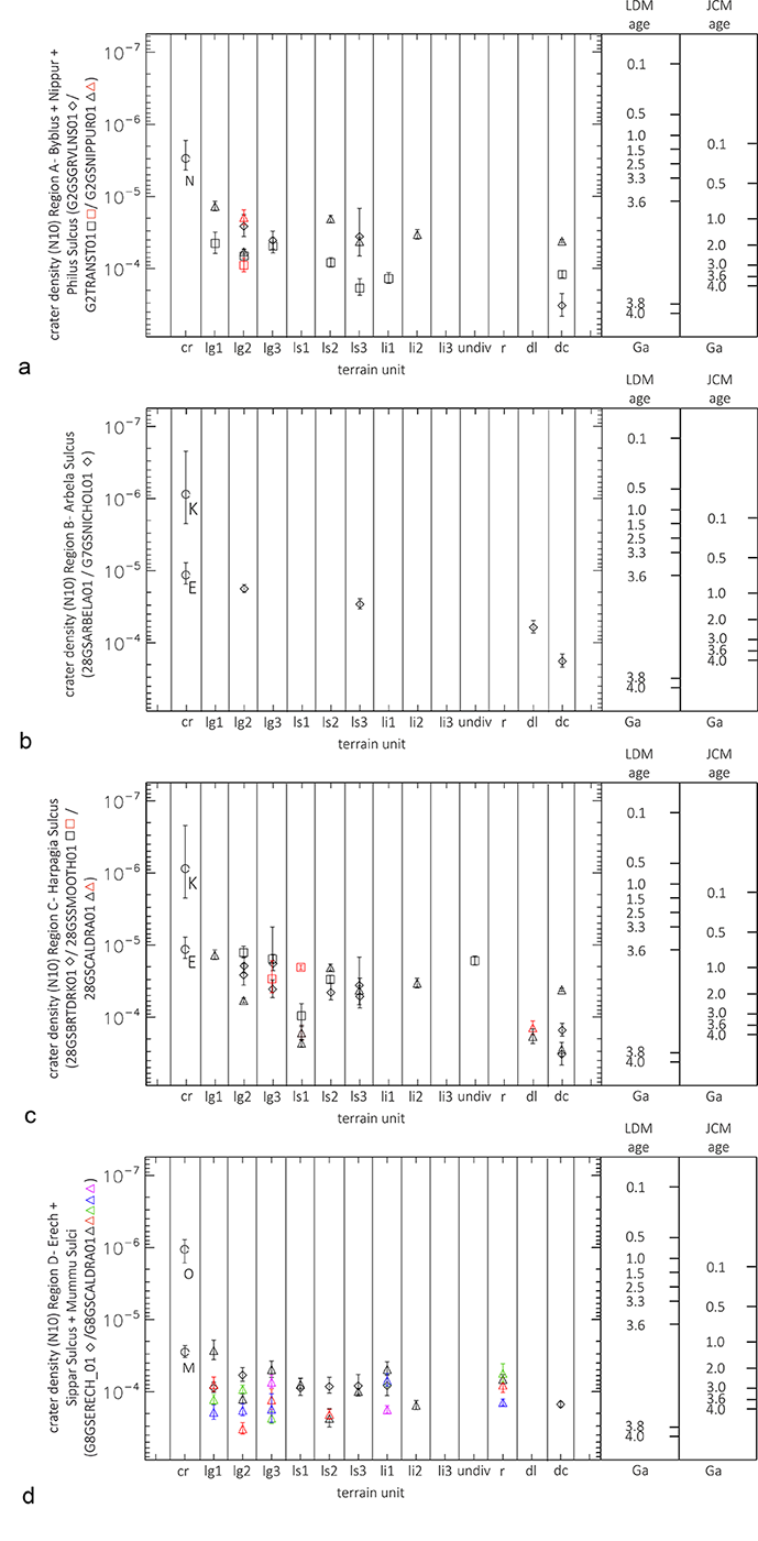
Figure 6: Stratigraphic correlation of Region a) A, b) B, c) C and d) D in which relative ages are determined by plotting the N(10) values with respect to each terrain units and corresponding ages based on LDM [7] and JCM [8]models. Please note that ages of fresh impact craters such as Nergal (N), Kittu (K), Enkidu (E), Melkart (M) and Osiris (O) have been added as additional stratigraphic markers. Since terrain types often appear more than one time in a geologic map the different facies are indicated by different colors.
References:
[1] Grasset, O., et al.: Planetary and Space Science, 78, 1-21, 2013. [2] Stephan, K., et al.: Planetary and space science, 208, 105324, 2021. [3] Pappalardo, R. T., et al.: Jupiter: The Planet, Satellites and Magnetosphere, 363-396, 2004. [4] Collins, G.C., et al.: Global geologic map of Ganymede (p. 3237), US Geological Survey, 2013. [5] Patterson, G. W. et al.: Icarus, 207, 845-867, 2010. [6] Baby, N. R., et al.: LPI Contributions, 2678, abstr. #1350, 2022. [7] Neukum, G., et al.: LPSC XXIX, abstr. #1742, 1998. [8] Zahnle, K., et al.: Icarus 163, 263-289, 2003. [9] Bland, M. T. et al. : Icarus 200, 207- 221, 2009. [10] Bottke et al.: LPSC, #2638, 2022.
How to cite: Baby, N. R., Stephan, K., Wagner, R., Kenkmann, T., Collins, G., Hauber, E., and Jaumann, R.: Stratigraphic relationships of different terrain units on Ganymede and possible implications towards their evolution, Europlanet Science Congress 2022, Granada, Spain, 18–23 Sep 2022, EPSC2022-1016, https://doi.org/10.5194/epsc2022-1016, 2022.
Icy bodies are the most numerous and diverse bodies in the Solar System, but only a few have been visited yet by space probes. Some of these icy bodies, mostly giant planet satellites like Callisto, are called ocean worlds as they likely host most of the liquid water of our Solar System within sub-glacial oceans [Sotin & Tobie 2004]. The presence of liquid water under the icy crusts of these bodies raises questions relative to exobiology. In the coming years and decades, these ocean worlds will be the focus of major planetary science missions, firstly with JUICE (ESA, launch scheduled in April 2023) and Europa Clipper (NASA, launch scheduled in October 2024) which will be targeting the Galilean moons, then with still conceptual missions as we speak such as (i) Uranus Orbiter and Probe and (ii) Enceladus Orbilander. Despite not being the prime target of any of these missions, Callisto will be investigated by JUICE and Europa Clipper through multiple flybys.
One way to get information about Callisto’s sub-glacial ocean is to look at the moon’s surface, which may highlight markers of past or current activity and could lift the veil on its chemical composition. Spectroscopy is a powerful technique for such study, especially in the near-infrared domain where spectral signatures of H2O-ices, silicates, salts are detectable. Consequently, in preparation for future infrared spectroscopic data, and specifically those of the infrared imaging spectrometer MAJIS of the JUICE mission, a ground-based campaign was led with an instrument sharing some similar and also complementary characteristics: SINFONI (SINgle Faint Object Near-infrared Investigation), which was mounted on the UT4 of the VLT at ESO. Here we present the results derived from the analysis and the modeling of four full-disk observations acquired with this instrument.
SINFONI combines an integral field spectrometer operating with different gratings with an adaptive optics module [Eisenhauer et al. 2003]. Our four observations were performed using the H+K grating, ranging from 1.46 µm to 2.41 µm, with a spectral resolution R = 1.500, but each spectrum acquired was automatically resampled in order to get a spectral sampling of 5 x 10⁻⁴ µm. The campaign took place from January 2015 from March 2016, and the observations were acquired near the opposition to optimize the angular resolution with Callisto’s angular diameter close to 1.5 arcsec. As SINFONI’s field of view is 0.8 x 0.8 arcsec2 divided into 64 x 64 pixels, one observation actually corresponds to a mosaic of ten overlapping acquisitions, as described in a paper about Ganymede using the exact same technique [Ligier et al. 2019]. All in all, after removing the high solar incident angle pixels we could not recover after applying photometric corrections (basically all pixels above latitude 60°, north and south), our dataset covers approximately 70% of Callisto’s entire surface with a spectral and spatial sampling (~40 km/pix) which allow to detect and map the spectral absorptions that may exist in this wavelength range of the Callisto’s spectrum. Spatial resolution is in par with that of the partial Callisto mosaic from the NIMS imaging spectrometer of the NASA Galileo probe.
The first results obtained concerns the physical properties of the moon’s surface directly derived from the reduction process and the photometric corrections; one obtains satisfactory results using the qualitative photometric model of Oren-Nayar, which is a generalization of the Lambertian model with the surface roughness (σ) as only additional parameter [Oren & Nayar 1994]. In the case of our study, the best results were obtained with ranging between 17° and 19° whatever the observation. These values are much lower than the values in the 30° – 45° range provided by previous studies [Buratti 1991, Domingue & Verbiscer 1997], however these values were obtained through the modeling of the solar phase curve via the Hapke model [Hapke 1984, Hapke 1986] using a combination of telescopic observations and Voyager data; the major differences between the approaches make the respective results hard to compare (our data are < 10° emergence angle).
Our second result concerns the global shape and spectral signatures in the surface spectra: overall, they are much flatter and more distorted than those of Europa and Ganymede, especially the quite large 2-µm H2O-ice band. To the exception of crystalline ice absorptions at ~1.50 µm, ~1.57 µm, ~1.65 µm and the 2-µm band, Callisto does not show other clear signatures (figure 1). However, very subtle signature(s), like the one at ~2.21 µm (figure 1), might actually be observed and are being investigated to confirm the detection(s). If confirmed it could suggest the presence of hydrated materials like salts or silicates. We will address this point during the meeting.
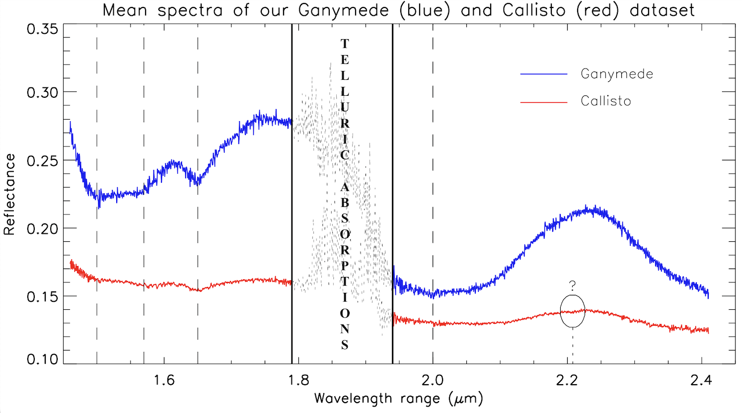
Figure 1: Comparison between Ganymede’s (blue) and Callisto’s (red) mean spectrum of the entire dataset.
And lastly our third main result comes from spectral modeling, where both linear and non-linear unmixing were performed. Unlike previous studies on Ganymede and Europa [Ligier et al. 2019, Ligier et al. 2016], the linear model shows that all of Callisto’s spectra are satisfactorily modeled without needing any hydrated salt and that the only two constituents would be (i) a darkening agent, with abundances always exceeding 80% even for the iciest spectra, and (ii) multiple grain sizes of the crystalline form of H2O-ice, with an average abundance of 7% and exhibiting a strong latitudinal gradient for the smallest grains typical of the influence of the Jovian magnetospheric environment (figure 2). Such a low concentration overall of H2O-ice challenged us about the legitimacy of the linear unmixing approach, so we decided to run the Shkuratov non-linear unmixing model [Shkuratov et al. 1999]. Tests are ongoing but very preliminary results show that the overall concentration of the crystalline ice should be much higher than the 7% coming from the linear model and hence much more representative of what should be the surface composition of an icy satellite. By the time of the meeting, we will be able to present the final results of the study.
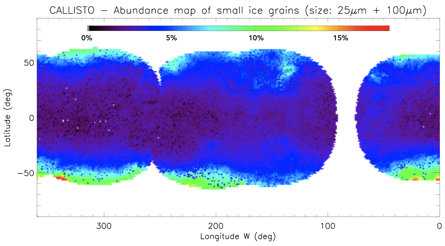
Figure 2: Distribution of the smallest grains of crystalline ice.
How to cite: Ligier, N., Riu, L., Carter, J., Calvin, W. M., Paranicas, C., and Poulet, F.: Pending the next "ocean worlds" missions: Callisto’s surface properties and composition from near-infrared telescopic data, Europlanet Science Congress 2022, Granada, Spain, 18–23 Sep 2022, EPSC2022-1050, https://doi.org/10.5194/epsc2022-1050, 2022.
The María de Maeztu Academy of the Centro de Astrobiología is a two year-long (2019-2020, 2020-2021), tailor-made capacity-building activity implemented within the frame of the “Maria de Maeztu” excellence programme. It aims to strengthen and develop new capacities and stimulate the training of young researchers. The first edition of the transdisciplinary challenges is a training activity of the María de Maeztu Academy intended to develope new skills and generating relevant scientific-technical solutions in the field of Astrobiology. The training program started in September 2021 by forming teams with volunteers from different CAB and INTA departments and different areas of expertise. Throughout 2020-2021, several periodic reviews of the proposals were carried out, passing different milestones and receiving expert comments in each evaluation. Then, the CAB’s MdM Executive Committee decided to financially support the four teams to develop the proposed projects in the 2021/2022 academic year, until the end of the María de Maeztu programme. One of those challenges is “NEXT (iN situ EXploration of planeTary objects): EUROPA” and its objective is to identify the optimal Raman technique for the exploration of the surface of Jupiter´s moon Europa in future missions:
- conducting tests of various Raman techniques (using both commercial and flight models) on representative samples from Europa
- characterizing these samples with the different Raman techniques
- generating a database of pros and cons of each technique, which can minimize risks and optimize expected results

Figure 1 - “NEXT (iN situ EXploration of planeTary objects): EUROPA” logo
In the search for life on other bodies within the Solar System, the top candidates are the icy moons, including Saturn’s moon Enceladus and Europa. These icy moons are target of study as they will help us in the task of assessing possible habitability zones in our neighborhood.
The choice of instruments that can answer these questions and also allow us to understand other factors is key. Raman spectroscopy has the versatility to be used to obtain those answers. It has been widely used in the analysis of terrestrial and planetary samples due to its advantages in rapid and non-destructive analysis of the mineralogy and mineral chemistry of rock and/or soil samples. For planetary explorations it exhibits great potentials for unambiguous phase identification due to its narrow and non-overlapping peak profiles, fast analysis without sample preparations, robust behavior and low mass, etc.
To achieve the stated objectives, a work plan has been established in different stages, subdivided into three phases:
- Samples preparation
- Tests conduction of various Raman techniques on the samples (first is carried out exclusively at the INTA facilities and in the second, the collaborating laboratories will take part)
- Analysis of the test results and database generation of pros and cons of each technique
The samples prepared consist in a saline solution with a molecular organic component. The salt used was MgSO4 that was detected by the Galileo mission [1]. The organic molecule selected was the amino-acid alanine. This amino-acid was discovering in several meteorites as the Murchison meteorite [2]. The sample solutions were prepared with proportions in weight of 5, 10 and 17 % for the salt, and 0.5, 1.0 and 1.5 for the alanine.
The following figures show the multisamples compositions of the nine samples (1 to 9), as a result of the prepared sample vials.

Figure 2 - Multisamples concentrations
Figure 3 - Prepared multisamples vials
In the second phase, the prepared samples will be analysed in liquid and frozen state with different Raman technologies in four laboratories including the ExoMars RLS [3] Flight Spare model located at INTA. RLS [4] was the first Raman spectrometer qualified for space applications. This phase will be completed in June 2022.
The laboratories where the tests will take place together with the Raman technology to be tested are as follows:
- Centro de Astrobiología (CAB): iHR550 Horiba with an in-situ 532nm laser and portable i-Raman BWTEK with an in-situ 532nm laser
- INTA: ExoMars RLS Flight Spare (in-situ visible green laser). GSE (control and scientific analysis) automated by SW
- University of Valladolid: Raman in-situ Exemplar® Plus LS High Performance Spectrometer with an 785nm (IR) laser and Raman with remote pulsed laser
- Instituto de Micro y Nanotecnología (IMN): LabRaman HR with two possibilities: 532 nm Solid State Diode Laser and 632 nm (HeNe) Solid State Diode Laser
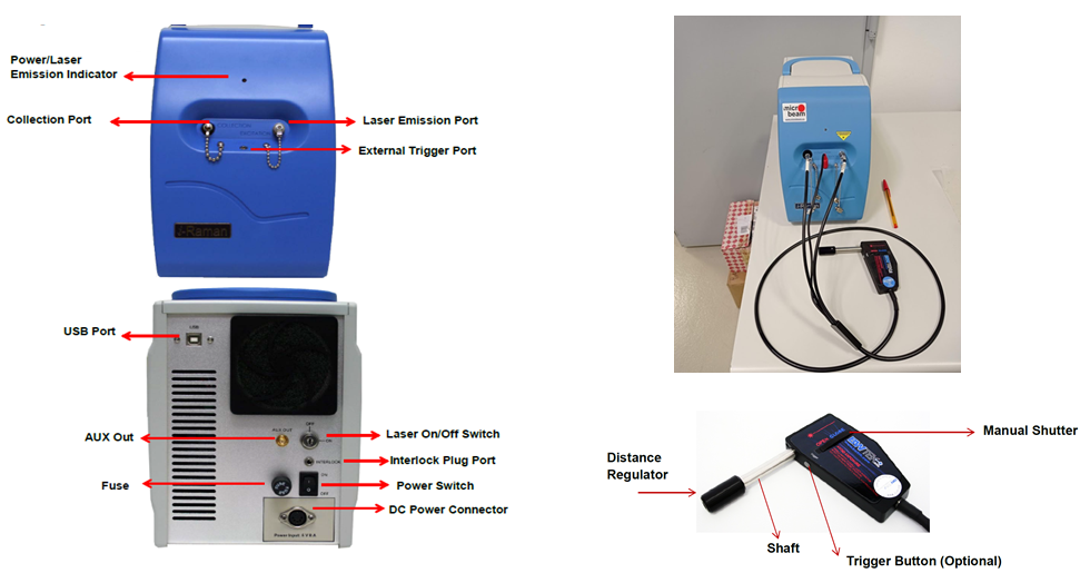
Figure 4 - portable i-Raman BWTEK at CAB facilities
Figure 5 - RLS Flight Spare Model at INTA facilities
With all the information provided by the Raman tests with Raman technology, an analysis of the results will be carried out in July 2022 and conclusions will be issued on the different techniques used to determine and argue which technology (remote or in-situ Raman technology, which excitation laser wavelength: visible / infrared spectrum) would be the most suitable for meet the scientific requirements to address whether life exists or has ever existed in Europa.
[1] Thomas B. McCord, Gary B. Hansen, Jean-Philippe Combe, Paul Hayne, Hydrated minerals on Europa’s surface: An improved look from the Galileo NIMS investigation, Icarus, Volume 209, Issue 2, 2010, Pages 639-650
[2] Engel, M., Nagy, B. Distribution and enantiomeric composition of amino acids in the Murchison meteorite. Nature 296, 837–840 (1982)
[3] Rull, F., et al, The Raman Laser Spectrometer for the ExoMars Rover Mission to Mars, Astrobiology, 2017, vol. 17(6-7), 627-654
[4] Moral, A.G., et al, A Raman Spectrometer for the ExoMars 2020 Rover, European Planetary Science Congress 2017, 17-22 September, 2017, Riga Latvia, id. EPSC2017-1001
How to cite: Zafra, J., Ercilla, O., Sanz, R., Benito, M., Rodriguez Prieto, J. A., Cabrero, J., Moral, A., Prieto Ballesteros, O., and Estrada, A.: “NEXT (iN situ EXploration of planeTary objects): EUROPA”, a challenge to identify the best Raman technique to explore the surface of Jupiter's moon Europa for future missions., Europlanet Science Congress 2022, Granada, Spain, 18–23 Sep 2022, EPSC2022-1088, https://doi.org/10.5194/epsc2022-1088, 2022.
OPS4 | Jupiter and Giant Planet System Science: New Insights From Juno
- Introduction and Summary
Jupiter’s troposphere is divided by eastward (prograding) jets into dynamical domains, which we number sequentially (Figure 1) so the highest-latitude northern domains are N4, N5 and N6 (Figure 2). Here we describe characteristics of these domains with short- and long-term tracking of features that can be identified in JunoCam images. Anticyclonic white ovals (AWOs) and cyclonic folded filamentary regions (FFRs) were tracked in 2021 and earlier years, using amateur images (analysed in the JUPOS project; e.g. Figure 3) and JunoCam maps (from the imager on NASA’s Juno orbiter; e.g. Figure 4) and several Hubble maps (from the OPAL project: ref.1).
The N6 domain is narrow and corresponds to a largely bland zone in JunoCam maps; all features in it are rapidly prograding. The N4 and N5 domains are broad and chaotic with numerous large FFRs and smaller vortices. Their zonal wind profiles (ZWPs) are dominated by the drifts of AWOs and FFRs, but faster retrograde winds exist in the FFRs. Northerly AWOs have rapid prograde drifts, but these often change suddenly, sometimes due to interactions with FFRs or with other AWOs. Most remarkably, in 2021-22 we have one or (very likely) two examples of AWOs moving south to cross prograde jets: one from the N4 domain and one from the N3 domain.
- Zonal drift profiles
Previous spacecraft ZWPs have revealed the overall pattern of the domains: in both N4 and N5, the ZWP is ‘blunt’ with a broad retrograde flow (Figure 1). The Cassini polar movie, and our long-term ground-based analysis [ref.2], suggested that this represents the bulk motion of the rapidly-changing FFRs, and this is confirmed by tracking features in 2021. The mean speeds in L3 are: in N4, +14 deg/30d; in N5, +20 deg/30d. Faster retrograde winds exist in the FFRs. Conversely, AWOs have fast prograding drifts when in the northern part of each domain, but steady retrograding drifts in the southern part, where they often wander in latitude (especially in N4). The largest AWO, in N5, has probably been tracked for at least 3 years and often progrades with the N6 jet. Some smaller AWOs are also long-lived, while others appear and disappear within months.
- Influences on the zonal drifts
In both N4 and N5, AWOs often undergo sudden large changes in their latitude and drift rate (Figure 3) – just as in the N2, S3 & S4 domains. Decelerations are sometimes due to the AWO encountering a FFR, according to examples in the Cassini polar movie and long-term ground-based analysis combined with Hubble maps [ref.2]. Accelerations may sometimes be due to the AWO encountering a smaller white spot. AWOs sometimes pass each other in different latitudes unperturbed, but sometimes their mutual interactions can lead to mergers, or cause one or both to change latitude and speed. In 2021, a pair in N5 rebounded exchang-ing tracks, and other interactions may have propelled a N4 and a N3 AWO southwards to cross the jet.
- AWOs crossing prograde jets
Coherent circulations almost never cross prograde jets on Jupiter, but ground-based data has demonstrated two previous instances where a N4 AWO crossed the N4 jet into the N3 domain, and in 2021-22 there was probably a third such event, captured in JunoCam images. N4-AWO-A swung rapidly southwards after it approached N4-AWO-B (Figures 3 & 4), and was last seen at PJ39, straddling the N4 jet and split into two lobes (Figure 4).
Likewise, a N3-AWO swung southwards and crossed the N3 jet into the NNTZ – the first time that a spot has been seen to cross a prograde jet other than the N4 jet.
- Cloud textures
JunoCam provides unprecedented resolution on the cloud-tops in this region, revealing features such as ‘pop-up clouds’; these are small, very bright white clouds only ten(s) of km across, projecting above the main cloud deck [ref.3], seen in many locations including AWOs, FFRs, and linear white cloud bands outside the main circulations (Figure 5). AWOs have thick white cloud cover with spiral streaking and scattered pop-up clouds. There are also much smaller vortices, both anticyclonic and cyclonic; the latter include well-formed orange-brown spiral cyclones, and ovals with quiescent dark brown cloud-covered interiors. FFRs have a variety of white, grey and orange clouds and hazes that appear to be at different levels. Dense rows of pop-up clouds are commonly seen on the white strips in FFRs, possibly representing the uppermost layer of convection. These white strips are probably thunderstorms, as FFRs in N4 are the most frequent location on the planet for lightning strikes [ref.4].
Acknowledgements: Some of this research was funded by NASA. A portion of this was distributed to the Jet Propulsion Laboratory, California Institute of Technology.
References:
1. Simon AA, Wong MH & Orton GS, NASA & ESA: OPAL project: https://archive.stsci.edu/prepds/opal/. See this website for maps and credits.
2. Rogers J et al., (2017), ‘Jupiter’s high northern latitudes: patterns and dynamics of the N3 to N6 domains.’ https://britastro.org/node/11328
3. Hansen C et al. (2019), ‘JunoCam images of castellanus clouds on Jupiter.’ AGU abstract #P44A-05.
4. Brown S et al.(2018), ‘Prevalent lightning sferics at 600 MHz near Jupiter’s poles.’ Nature 558, 87-90.


How to cite: Rogers, J., Adamoli, G., Hansen, C., Eichstädt, G., Orton, G., Momary, T., Jacquesson, M., Bullen, R., and Mettig, H.-J.: Jupiter’s high-latitude northern domains: Dynamics from Earth-based and JunoCam imaging, Europlanet Science Congress 2022, Granada, Spain, 18–23 Sep 2022, EPSC2022-16, https://doi.org/10.5194/epsc2022-16, 2022.
The study of Jupiter’s atmosphere, its composition, evolution, distribution, structure, and dynamics around the planet, is of interest to the scientific community. Several missions, space observatories, and ground-based telescopes (even if limited by the telluric bands of water vapor), have studied Jupiter’s atmosphere. Some of them, such as Juno, the Hubble Space Telescope (HST), and the Very Large Telescope (VLT), continue providing information about the vertical structure and distribution of the atmosphere around the planet [1-3]. Although the main chemical composition of Jupiter’s atmosphere has been unraveled, many questions remain open, such as the global abundance of water, or the responsible chemistry for the coloration of the clouds [4]. Besides, a remarkable potential of VIS-NIR spectrometry for characterizing the composition and dynamics of planetary atmospheres has been demonstrated in the last years [5].
The next mission to the Jovian system from the European Space Agency (ESA) is the Jupiter Icy Moons Explorer (JUICE), to be launched in April 2023 with an arrival date on July 2031 [6]. One of the key scientific instruments onboard is the Moons And Jupiter Imaging Spectrometer (MAJIS), which will provide hyperspectral capabilities through two channels: VIS-NIR (0.5μm-2.35μm), and IR (2.25μm-5.54μm) [7]. We would like to perform simulations of different test cases with respect to the viewing geometries of MAJIS and assess its capabilities [8-9] to characterize the vertical structure of the Jovian atmosphere. For this purpose, we upgraded ASIMUT-ALVL, a Radiative Transfer (RT) code developed at BIRA-IASB, that has been extensively used to characterize Mars and Venus atmospheres [10-11].
During the implementation phase of the new Jupiter case in ASIMUT-ALVL, we applied the current knowledge of the physical and chemical characteristics of Jupiter, including the Rayleigh scattering contribution due to dominant atmospheric species, the refractive index of Jupiter’s atmosphere, and the Collision-Induced Absorption (CIA) due to H2-H2 and H2-He molecular systems. The typical temperature profile and atmospheric composition of Jupiter were retrieved from [12], although in our next studies we might use the CH4 abundance from the Volume Mixing Ratio (VMR) profile from [13], which is similar to that from [14]. The required line-lists were implemented from the HITRAN online database with line parameters adequate for an H2 and He dominant atmosphere, following the 2020 version release [15]. The extinction coefficient due to Rayleigh Scattering is obtained based on the calculation of its cross-section from [16], by considering the refractive indexes of H2 and He, obtained from the refractivities measured by [17] and [18], respectively. The atmospheric King correction factor is obtained from an adapted version of the formula of [19], considering the depolarization ratio of H2 as measured by [20]. To model the aerosols and hazes present in the atmosphere, we used the microphysical parameters defined by [21].
We validated the updated performances of ASIMUT-ALVL by individually comparing the main spectroscopic features of Jupiter’s atmosphere in the VIS-NIR range against KOPRA, an RT code originally developed for studying Earth’s atmosphere but later adapted to the atmospheres of Titan, Mars, and Jupiter [22]. We used the same geometry of observation, assuming solar occultations with a tangential altitude between 50km and 360km, a resolution of 0.3cm-1, a Signal-to-Noise Ratio (SNR) of 100, and an orbit around the planet of 5000km high. The mean difference in transmittance obtained between both models is below 3%.
The next step was to validate our RT model against observational spectroscopic data, which was obtained from the Visible and Infrared Mapping Spectrometer (VIMS) observations during the Cassini flyby to Jupiter [23]. This imaging spectrometer consists of two channels: VIS (0.35µm-1.07µm) and IR (0.85µm-5.1µm). In this presentation, we will discuss the results we obtained from the complete validation of our RT model, and the perspectives for the future implementation of the performances and viewing geometries of MAJIS/JUICE.
Acknowledgements
We acknowledge the kind support of Gianrico Filacchione who provided the calibrated data of the VIMS/Cassini observations. This project also acknowledges the funding provided by the Scientific Research Fund (FNRS) through the Aspirant Grant: 34828772 MAJIS detectors and impact on science.
References
[1] Bolton, S.J., et al., Space Science Reviews, 2017. 213(1): p. 5-37.
[2] Nichols, J.D., et al., Geophysical Research Letters, 2017. 44(15): p. 7643-7652.
[3] Antuñano, A., et al., The Astronomical Journal, 2019. 158(3): p. 130 (28).
[4] MAJIS Team, JUICE Definition Study Report, 2014.
[5] Langevin, Y., et al., Lunar and Planetary Science Conference, 2014. No. 1777: p. 2493.
[6] Grasset, O., et al., Planetary and Space Science, Vol. 78, pp. 1-21, 2013.
[7] Piccioni, G. et al., International Workshop on Metrology for AeroSpace, IEEE, 2019. pp. 318-323.
[8] ESA, Consolidated Report on Mission Analysis (CReMA), Tech. Rep. 5.0b23.1. https://www.cosmos.esa.int/web/spice/spice-for-juice
[9] Cisneros-González, M. E. et al., Space Telescopes and Instrumentation in Proc. SPIE 2020, 11443, 114431L.
[10] Vandaele, A.C., et al., Planetary and Space Science, 2015. 119: p. 233-249.
[11] Vandaele, A.C., et al., Optics Express, 2013. 21(18): p. 21148-21161.
[12] Moses, J.I., et al., Journal of Geophysical Research: Planets, 2005. 110(E8).
[13] Sánchez-López, et al., Astronomy & Astrophysics, 2022. Forthcoming article (ArXiv:2203.10086).
[14] Seiff, A., et al., Journal of Geophysical Research: Planets, 1998. 103(E10): 22857-22889.
[15] Gordon, I.E., et al., Journal of Quantitative Spectroscopy and Radiative Transfer, 2022. 277: p. 107949.
[16] Sneep, M., et al., Journal of Quantitative Spectroscopy and Radiative Transfer, 2005. 92(3): p. 293-310.
[17] Peck, E.R. et al., Journal of the Optical Society of America, 1977. 67(11): p. 1550-1554.
[18] Mansfield, C.R., et al., Journal of the Optical Society of America, 1969. 59(2): p. 199-204.
[19] Tomasi, C., et al., Applied optics, 2005. 44(16): p. 3320-3341.
[20] Parthasarathy, S., Indian Journal of Physics, 1951. 25: p. 21-24.
[21] López-Puertas, M., et al., The Astronomical Journal, 2018. 156.4: 169.
[22] Stiller, G.P., et al., Optical Remote Sensing of the Atmosphere and Clouds, SPIE 2000, 3501.
[23] Brown, R.H., et al., Icarus, 2003. 164(2): p. 461-470.
How to cite: Cisneros González, M. E., López-Puertas, M., Erwin, J., Vandaele, A. C., Lauzin, C., Poulet, F., and Robert, S.: Validation of ASIMUT-ALVL against observational data of Jupiter’s atmosphere, Europlanet Science Congress 2022, Granada, Spain, 18–23 Sep 2022, EPSC2022-145, https://doi.org/10.5194/epsc2022-145, 2022.
Jupiter's stratospheric chemistry and dynamics are poorly understood as a function of latitude. The Shoemaker-Levy 9 comet impacts in Jupiter's atmosphere in 1994 have offered us with a unique means to characterize Jupiter's stratospheric chemistry and dynamics. We can indeed use the delivery at 44°S of the long-lived species HCN, CO, H2O, and CS and the subsequent temporal evolution of their spatial distribution as constraints for vertical and meridional mixing, zonal winds and chemistry as a function of latitude.
We mapped HCN and CO in Jupiter's stratosphere with ALMA in March 2017. These observations have already been used in Cavalié et al. (2021) and Benmahi et al. (2021) to derive the stratospheric zonal wind field. In this paper, we use the same observations to retrieve the vertical and meridional distributions of HCN and CO, almost 25 years after the comet impacts. We will present the spatial distributions of both species and discuss the implications on Jupiter's stratospheric chemistry, and vertical and horizontal mixing.
How to cite: Cavalié, T., Rezac, L., Moreno, R., Lellouch, E., Fouchet, T., Benmahi, B., Greathouse, T. K., Sinclair, J. A., Hue, V., Hartogh, P., Dobrijevic, M., Carrasco, N., and Perrin, Z.: ALMA observations of the spatial distribution of CO and HCN in the stratosphere of Jupiter, Europlanet Science Congress 2022, Granada, Spain, 18–23 Sep 2022, EPSC2022-355, https://doi.org/10.5194/epsc2022-355, 2022.
At Jupiter, magnetosphere-ionosphere coupling gives rise to intense auroral emissions and enormous energy deposition in the magnetic polar regions. Here we show ground-based maps of Jupiter's upper atmosphere temperatures obtained via the emissions of the major upper-atmospheric ion, H3+. The maps have a spatial resolution of 2o longitude and latitude from pole to equator and trace the global temperature gradient. We find that temperatures decrease steadily from the auroral polar regions to the equator, indicating that the aurora act as a planet-wide heating source. However, during a period of enhanced activity in the auroral region which models imply was due to a solar wind compression, a high-temperature planetary-scale-sized structure was also observed on top of this gradient. This presentation reports on the particulars of this feature, including how it appears to be propagating away from the main auroral oval (as determined by estimates of the features' velocity at several longitudes) and its subsequent implications for global energy circulation at Jupiter and other planets.
How to cite: O'Donoghue, J., Moore, L., Bhakyapaibul, T., Johnson, R., Melin, H., and Stallard, T.: A planetary-scale heat wave in Jupiter's mid-latitude upper atmosphere, Europlanet Science Congress 2022, Granada, Spain, 18–23 Sep 2022, EPSC2022-373, https://doi.org/10.5194/epsc2022-373, 2022.
Ground- and space-based remote sensing, from Voyager, to Galileo, Cassini and Juno, has revealed the existence of circulation cells in the troposphere of Jupiter. These circulation cells, which may be similar to terrestrial Ferrel cells [1], show properties that vary significantly as a function of depth, showing circulations of opposing directions above and below the expected level of the water condensation cloud near 4-6 bar [2]. Moreover, the location of each vertical branch of the Ferrel-like cells are correlated to the Jupiter's temperature belt/zone contrast, suggesting a dynamical and thermal link between winds, temperatures, aerosols, and composition.
To provide infrared support for Juno spacecraft observations, we have been observing Jupiter with the VISIR mid-infrared instrument on the Very Large Telescope (VLT) since 2016. We analyse images at multiple wavelengths between 5 and 20 µm to study the thermal, chemical and aerosol structure of Jupiter's belts, zones, and polar domains. In particular, an observing run in May 2018 (conciding with Juno's 13 perijove) provided global coverage of Jupiter in thirteen narrow-band filters. These data sense stratospheric temperature (7.9 µm), tropospheric temperature via the collision-induced hydrogen-helium continuum (13, 17.6, 18.6, 19.5 µm), aerosol opacity (8.6 and 8.9 µm), and the distribution of ammonia gas (10.5, 10.7 and 12.3 µm). These wavelengths primarily sound the upper troposphere at p<0.7 bar, above the cloud tops, so are sensitive to the upper cell of the belt/zone Ferrel-like circulations. By stacking the data in all 13 filters, we invert the data using the optimal-estimation retrieval algorithm NEMESIS [3] to derive temperature, aerosol and chemical structure over the whole planet. Meridional gradients of temperature, wind shear (derived from thermal balance equation) and chemical species will be examined to understand the upper-tropospheric circulation cells.
We confirm that the pattern of cool anticyclonic zones and warm cyclonic belts persists throughout the mid-latitudes, up to the boundary of the polar domains. This implies, via thermal wind balance, the decay of the zonal jets as a function of altitude throughout the upper troposphere. Aerosol opacity is often (but not always) highest in the anticyclonic zones, suggesting condensation of saturated vapours, but we caution that aerosol opacity is not a good proxy for atmospheric circulation on any giant planet. The thermal and compositional gradients derived from the VISIR maps are consistent with those from Voyager and Cassini, but opposite to what would be inferred for the Ferrel-like circulations of the deeper cell of [1], which was suggested by [2] to exist only below the water-cloud layer based on Juno microwave observations.
Concerning the Jovian polar regions, the analysis of VISIR imaging shows a large region of mid-infrared cooling poleward ~67˚S, co-located with the reflective aerosols observed in methane-band imaging by JunoCam, suggesting that they play a key role in the radiative cooling at the poles, and that this cooling extends from the upper troposphere into the stratosphere. These VISIR observations also reveal thermal contrasts across polar features, such as numerous cyclonic and anticyclonic vortices, as well as evidence of high-altitude heating by auroral precipitation. Comparison of zonal mean thermal properties and high-resolution visible imaging from Juno allows us to study the variability of atmospheric properties as a function of altitude and jet boundaries, particularly in the cold southern polar vortex. To investigate the radiative processes and influence of auroral precipitation on the southern cold vortex, a radiative-convective model tailored for Jupiter's atmosphere [4], with an updated polar aerosol distribution from Juno mission results, will be used to determine the aerosol distribution needed to reproduce the thermal structure of the cold polar vortex of Jupiter.
[1] Duer, K., Gavriel, N., Galanti, E., Kaspi, Y., Fletcher, L. N., Guillot, T., Bolton, S. J., Levin, S. M., Atreya, S. K., Grassi, D., Ingersoll, A. P., Li, C., Li, L., Lunine, J. I., Orton, G. S., Oyafuso, F. A., Waite, J. H.: Evidence for Multiple Ferrel-Like Cells on Jupiter, Geophysical Research Letters, 2021.
[2] Fletcher, L. N., Oyafuso, F. A., Allison, M., Ingersoll, A., Li, L., Kaspi, Y., Galanti, E., Wong, M. H., Orton, G. S., Duer, K., Zhang, Z., Li, C., Guillot, T., Levin, S. M., Bolton, S: Jupiter's Temperate Belt/Zone Contrasts Revealed at Depth by Juno Microwave Observations, Journal of Geophysical Research: Planets, 2021
[3] Irwin, P. G. J., Teanby, N. A., de Kok, R., Fletcher, L. N., Howett, C. J. A., Tsang, C. C. C., Wilson, C. F., Calcutt, S. B., Nixon, C. A., Parrish, P. D.: The NEMESIS planetary atmosphere radiative transfer and retrieval tool, Journal of Quantitative Spectroscopy & Radiative Transfer, 2008
[4] Guerlet, S., Spiga, A., Delattre, H., Fouchet, T.: Radiative-equilibrium model of Jupiter's atmosphere and application to estimating stratospheric circulations, Icarus, 2020
How to cite: Bardet, D., Donnelly, P., Fletcher, L. N., Antuñano, A., Roman, M. T., Orton, G. S., Guerlet, S., Melin, H., and Harkett, J.: Investigating Thermal Contrasts Between Jupiter's Belts, Zones, and Polar Vortices with VLT/VISIR, Europlanet Science Congress 2022, Granada, Spain, 18–23 Sep 2022, EPSC2022-535, https://doi.org/10.5194/epsc2022-535, 2022.
In 2012, ground-based observations of the dominant molecular ion in gas giant ionospheres, H3+, found that Jupiter’s upper atmosphere was super-heated above its iconic Great Red Spot (GRS). Temperatures there reached 1600 K, hotter even than the auroral region. It was speculated that this GRS “hotspot” was the signature of coupling between Jupiter’s lower and upper atmosphere, perhaps associated with upward propagating acoustic or gravity waves originating from the Solar System’s most powerful storm system. Such an energy transfer could help explain why observed upper-atmospheric gas giant temperatures are all significantly warmer than simulations based solely on solar heating can explain, a discrepancy colloquially referred to as the “giant planet energy crisis”.
Here, based on ground-based observations from 2016-2019, we report on spatial and temporal variations of H3+ temperature surrounding the GRS. We find that, while upper-atmospheric temperatures are still elevated above the GRS, they vary in time and are significantly cooler than in 2012. In addition, there are consistent spatial variations, with H3+ temperature generally highest on the western and northern edges of the GRS. We place these results in context with recent work that implicates Jupiter’s aurorae as primary sources of upper-atmospheric heating, and comment on their implications for Jupiter’s energy crisis.
How to cite: Moore, L., Stallard, T., O'Donoghue, J., Melin, H., Chowdhury, M. N., Johnson, R., Vogt, M., Schmidt, C., and Orton, G.: Ionospheric temperature variability above Jupiter’s Great Red Spot, Europlanet Science Congress 2022, Granada, Spain, 18–23 Sep 2022, EPSC2022-564, https://doi.org/10.5194/epsc2022-564, 2022.
The grand appearance of Jupiter’s banded atmosphere, coloured with many shades from white to red, whose cloud structure currently remains elusive with no clear single cloud model responsible for this varied appearance. With a general pattern of alternating bright cloudy zones and darker belts, as well as unique regions such as the Great Red Spot, finding a way to model all of these differing appearances with a single model has proven difficult. Jupiter’s atmosphere provides continual challenges when attempting to characterise its cloud structure due to its frequently varying appearance. This leads to differences between every observation meaning that models are constantly having to adapt to be explain these changes. Such changes can be seen in Figure 1, both of these spectra have been extracted for the same region of the Equatorial Zone (EZ) but are not identical due to the changes in appearance over the 3 years.
Recent works [1,2,3,4] have all attempted to model Jupiter’s atmosphere using a universal chromophore (cloud colouring compound), combined with a deeper conservatively-scattering cloud and also a stratospheric haze layer. These works have all been able to model the atmosphere successfully but it has currently not been possible to determine between these differing solutions to find the most likely representation of the atmosphere. As all the different sets ups have several ways to vary cloud structure and chromophore properties among other parameters, they have been able to fit the changes in the observations. Therefore keeping each set up viable even as the atmosphere changes. The current inability to conclude on a favoured cloud structure highlights the highly degenerate nature of this problem.
Utilising new observations and techniques to analyse the data highlights the delicacy of these results as the previous set ups have to be altered in order to produce the desired fit to the new observations once the input have varied slightly. An unchanged fit is shown in Figure 1, where the ideal fit of the EZ in 2018 has been used for 2021 data and is unable to model the spectra as well as for the spectra which it was derived from. Furthermore introduction of a limb viewing technique, as used in [2], has been done for this data. Here we attempt to fit multiple viewing angles simultaneously, which also begins to question the robustness of these results, due to an inability of nadir derived set ups to reproduce the multiple observations as successfully.
Therefore in this work we have begun to attempt to reduce the degeneracy of the problem before utilising the Non-linear optimal Estimator for Multi-variatE spectral analySIS (NEMESIS) radiative-transfer retrieval algorithm [5], to fit to our observations. From this we want to find a vertical cloud structure which is more reproducible using different observations and techniques. It is hoped that reducing one of the degenerate parameters before fitting will allow us to constrain the atmospheric structure more decisively. Furthermore combining this with the limb darkening technique will hopefully allow us to rule out some of the solutions to this highly degenerate problem to find more confidence in the proposed models.
In this work we will present the preliminary results taken from the application of these methods to observations to derive a new atmospheric model which can be compared with past work. Additionally we will present the use of new techniques to determine the ability of previous models to adapt to new observations to see if they are still viable.

Figure 1: Spectra of the Equatorial Zone in both 2018 and 2021 and the spectral fit using the model from [1] derived for the 2018 data.
[1] Braude, A. S., Irwin, P. G., Orton, G. S., and Fletcher, L. N. (2020). Colour and tropospheric cloud structure of jupiter from muse/vlt: Retrieving a universal chromophore. Icarus, 338:113589.
[2] Pérez-Hoyos, S., Sánchez-Lavega, A., Sanz-Requena, J., Barrado-Izagirre, N., Carrión-González, O., Anguiano-Arteaga, A., Irwin, P., and Braude, A. (2020). Color and aerosol changes in jupiter after a north temperate belt disturbance. Icarus, 352:114031.
[3] Dahl, E. K., Chanover, N. J., Orton, G. S., Baines, K. H., Sinclair, J. A., Voelz, D. G., Wijerathna, E. A., Strycker, P. D., and Irwin, P. G. J. (2021). Vertical structure and color of jovian latitudinal cloud bands during the juno era. The Planetary Science Journal, 2(1):16.
[4] Baines, K., Sromovsky, L., Carlson, R., Momary, T., and Fry, P. (2019). The visual spectrum of jupiter’s great red spot accurately modeled with aerosols produced by photolyzed ammonia reacting with acetylene. Icarus, 330:217–229.
[5] Irwin, P. G. J., Teanby, N. A., de Kok, R., Fletcher, L. N., Howett, C. J. A., Tsang, C. C. C., Wilson, C. F., Calcutt, S. B., Nixon, C. A., and Parrish, P. D. (2008). The NEMESIS planetary atmosphere radiative transfer and retrieval tool. , 109:1136–1150
How to cite: Alexander, C. and Irwin, P.: Comparing atmospheric models of Jupiter, can we reduce the degeneracy of this problem?, Europlanet Science Congress 2022, Granada, Spain, 18–23 Sep 2022, EPSC2022-632, https://doi.org/10.5194/epsc2022-632, 2022.
The Juno Microwave Radiometer (MWR) has extended our knowledge of the structure and composition of Jupiter's atmosphere down to several hundred bars, revealing meridional variability at great depths (e.g. Li et al. 2017, Fletcher et al. 2021). It has revealed that some cyclonic and anticyclonic vortices may have roots at depths of hundreds of bars of pressure (Bolton et al. 2022), but 5-µm hot spots and associated plumes are restricted to shallow depths above the water cloud (Fletcher et al. 2021). We report ongoing work on evolution of axisymmetric bands, concentrating on two regions where large-scale changes have been observed in the visible and infrared.
One of these is the Equatorial Zone (EZ), for which Figure 1 illustrates a dramatic color change. The color change in the central component (EZc, ~3°S – 1°N, planetocentric latitude) is more prominent than the northern component (EZn, ~2° - 6°N). This change began in 2018, and by 2019 was as prominent as shown in 2021. In near-infrared bands of strong gaseous absorption, the EZc reflectivity increased dramatically (Fig. 2), but only temporarily for the EZn.
Another region is the northern component of the North Equatorial Belt (NEBn, ~12°N to 15°N), whose change from a visibly dark to a bright region is also illustrated in Figure 1, with the southern component (NEBs, ~7°N to 11°N) remaining its typical dark color. Figure 3 shows that this color is associated with a remarkable drop of its 5-µm brightness which dropped down to the faint emissions of the nearby cloudy and visually bright zones. This implies a major increase in the opacity of 0.7-5 bar clouds that are similar but more extreme than the quasi-periodic northward expansions of the NEB (Fletcher et al. 2017). This transformation took place in early 2021 when Jupiter was in solar conjunction.
The very preliminary results of our initial examination of MWR observations (Fig. 4) plot antenna temperatures derived using averages over all longitudes sensed in which the center of the field of view lay within specified latitude ranges. Observations were selected only if 99% or more of the field of view included the planet and the emission angle was limited to 65° or less, after which they were converted to a nadir-equivalent emission using limb-darkening models that were fit to every latitude and each channel. All observations were made at close approaches of the spacecraft to Jupiter, known as ‘perijoves’ or PJs. Many perijoves between 2019 and 2022 did not contain any measurements of these regions meeting those selection criteria, due to unfavorable spacecraft pointing. Exceptions included special spacecraft orientations.
The EZc appears invariable in time, but the EZn underwent a ~7K drop in Channel-3 antenna temperatures - sensitive to conditions near ~9 bars - starting in early 2017, reaching a minimum in late 2017, then returning to its original values by early 2019. Similar variability is evident in Channel 4, sensitive to the ~3-bar level, and a smaller one in Channel 5, which is sensitive to the ~1.5-bar level. No change is detectable in Channel 6, sensitive to the ~0.7-bar level. The 2017 temperature drop has no obvious counterpart in reflected sunlight, although its “recovery” occurs during the reflectivity changes in 2019 (Figs. 1-2). To link the two, one must devise a causal relationship between a short-lived variation of absorber, likely gaseous ammonia, at 1.5-9 bars at 2016-2019 between 2°N and 6°N, and conditions at higher altitudes over a wider latitude range.
If the NEBn variability between 2020 and 2021 (Figs. 1, 3) implies an increase of ammonia absorption, we would expect a decrease in antenna temperatures between our last trustworthy observation in 2019 April and observations in late 2021. This is indeed the case at 0.7 bars, represented by the 6-7K drop in Channel-6 antenna temperatures for the NEBn. This is also present in Channel 5 as a ~5K drop, but it is not detectable above the noise in the deeper-sounding channels, so this is not substantially present at pressures higher than ~1.5 bars. A ~5K drop in antenna temperatures in late 2016 is followed by a slower rise to its previous range by the end of 2017 in both Channels 5 and 6. Other channels do not show this variability, so this is another “shallow” phenomenon with no obvious connection to changes in cloud reflectivity.
We will continue to examine variability in cloud reflectivity associated with these changes, observe with increasingly favorable geometries for the next few perijoves, and examine other latitudes for variability.
References:
Bolton, et al. 2021. Science 374, 968-972.
Fletcher, et al. 2017. Geophys. Res. Lett. 44, 7140-7148
Fletcher, et al. 2020. J. Geophys. Res. 125, E06399.
Fletcher, et al. 2021. J. Geophys. Res. 126, E06858.
Li, et al. 2017. G. Res. Lett. 44, 5317-5325.
Simon, et al. 2015. Ap. J. 812, 55.

Figure 1. Color-composite cylindrical maps of Jupiter from the Hubble Space Telescope OPAL program (Simon et al. 2015). Note the darkening of the EZ central and northern components, which began in 2018. Note also that in 2021 the northern part of the North Equatorial Belt has become lighter in color compared with 2017, a process that took place in early 2021.

Figure 2. Reflectivity of the central and northern components of the Equatorial Zone vs time at 2.166 µm, a wavelength sensitive to reflected sunlight from ~80-mbar aerosols. This plot implies that the EZn contained a denser population of aerosols near this level, most likely from more vigorous lofting.

Figure 3. Images of Jupiter at 5.1 µm: these and data in Fig. 2 were taken using NASA’s Infrared Telescope Facility (IRTF) SpeX guide camera. Note the drop in radiance of the northern section of the North Equatorial Belt from 2020 to 2021.

Figure 4. Preliminary results on radiances measured by Juno’s Microwave Radiometer (MWR). Channels 3 and 6 sense radiances at 2.6 and 22 GHz, respectively. For clarity, other channels are not shown. Error bars represent the standard deviation of antenna temperatures included in the latitude bin.
How to cite: Orton, G., Fletcher, L., Oyafuso, F., Li, C., Zhang, Z., Brueshaber, S., Wong, M. H., Momary, T., Levin, S., Bolton, S., Baines, K., Dahl, E., and Sinclair, J.: Exploring the Depth of Planetary-Scale Changes in Jupiter from Juno Microwave Radiometer Observations, Europlanet Science Congress 2022, Granada, Spain, 18–23 Sep 2022, EPSC2022-761, https://doi.org/10.5194/epsc2022-761, 2022.
Since 2016 the Juno spacecraft has been in orbit around Jupiter, gathering unprecedented data from its highly inclined 53-day orbit. The Jupiter Infrared Auroral Mapper (JIRAM) is an imager and spectrograph with spectral coverage between 2 and 5 µm. This region is dominated by reflected sunlight by aerosols and hazes, with distinct absorptions by ammonia, phosphine, germane and other minor species in Jupiter's troposphere, as well as ionospheric H3+ at high altitude. Here, we outline the process undertaken to model the full spectral coverage of JIRAM with NEMESIS, our radiative transfer and retrieval code (Irwin et al., 2008). This includes altering the NH3 aerosol and haze properties, updating the molecular line-list, and testing the sensitivity to the abundance of the molecular species that are within the 2-5 µm range offered by JIRAM.
This study builds on previous models for JIRAM spectra in thermal emission (Grassi et al., 2020) and reflected sunlight (Grassi et al., 2021), by attempting to fit the entire 2-5 µm range simultaneously with a single consistent aerosol model. The model includes two aerosol layers, a NH4SH type layer at 1.3 bars, and a NH3 type layer at 0.7 bars, as well as a tholin type haze layer that extends from the troposphere to the stratosphere. We demonstrate that JIRAM observations of both reflected sunlight and thermal emission cannot be reproduced simultaneously using standard refractive indices available in the literature. We build a simple model of the refractive indices for the three aerosol layers, adapting the technique of Sromovsky et al. (2010), and demonstrating the improvement in the fits at each step. As a proof of concept we present the analysis of meridionally averaged zonal profiles, investigating how aerosols, ammonia, and phosphine vary with latitude during the early perijoves of the mission.
How to cite: Melin, H., Fletcher, L., Irwin, P., Grassi, D., and Mura, A.: Modelling the full 2-5 µm Juno JIRAM spectral range with NEMESIS: Zonal Profiles of Jupiter’s Aerosols, Condensables, and Disequilibrium Species, Europlanet Science Congress 2022, Granada, Spain, 18–23 Sep 2022, EPSC2022-817, https://doi.org/10.5194/epsc2022-817, 2022.
The shape of gaseous planets, defined as an equipotential surface for a specific pressure, can be calculated given measurements of the zonal gravity harmonics, and the wind profile and polar radius at a given level. For both Jupiter and Saturn, the gravity harmonics have been measured to high accuracy by the Juno and Cassini missions, respectively. Measurements for the zonal winds are also available via cloud tracking, buth a significant uncertainty is associated with them, stemming from the clouds altitudes, as well as time variations in the strength and location of the winds. With that, the wind profiles can be also constrained by the gravity measurements. Further constraint on the calculated shape of the two gas giants can be obtained from occultation measurements, which give radial dependent profiles of pressure for specific spatial location.
Here we propose a new method for calculating the shape of the gas giants, based on an optimization of the wind latitudinal profile, decay structure, and the polar radius, given both gravity and occultation measurements. We use thermal wind balance to relate the wind to the gravity measurements, and a shape model to relate the wind and polar radius to the occultation measurements. We perform the analysis for both the 0.1 and 1 bar pressure levels. We examine the ability to explain both types of measurements in each planet, and discuss the implication for the possible wind profiles and how they might change with pressure. We also discuss the solutions for the polar radius with respect to the currently used mean values.
Only a few occultation measurements are currently available in each planet, but in the coming years the Juno mission is expected to perform dozens of occultations for Jupiter, covering a wide spatial range, and there are several Cassini occultations performed for Saturn that are still waiting for analysis. Using the method proposed here, we expect the new measurements to help resolve the shape of the gas giants to better accuracy, and to allow better understanding of the wind structures and their depth dependence.
How to cite: Galanti, E., Smirnova, M., Kaspi, Y., and Guillot, T.: The shape of Jupiter and Saturn based on winds, occultations and gravity measurements, Europlanet Science Congress 2022, Granada, Spain, 18–23 Sep 2022, EPSC2022-843, https://doi.org/10.5194/epsc2022-843, 2022.
A key feature among the Galilean satellites is their monotonic decrease in density, indicating an ice fraction that is zero in the innermost moon Io, and about half in the outer moons Ganymede and Callisto. So far, there is no formation scenario that explains this gradient while considering the moons grew in a water-depleted circumplanetary disk. Here, we investigate the possibility that the jovian circumplanetary disk was fueled with ice-free chondritic minerals, including phyllosilicates. To do so, we use a standard one-dimensional gas-starved accretion disk model derived from the literature [1, 2] coupled with gas and solids transport modules [3, 4] to investigate the evolution of vapors released by the dehydration of phyllosilicates. We show that the dehydration of such particles and the outward diffusion of the released water vapor allows condensation of significant amounts of ice in the formation region of Ganymede and Callisto in the Jovian circumplanetary disk. This mechanism naturally explains the presence of ice-rich moons around a water-depleted Jupiter.
[1] Canup, R.M., Ward, W.R. 2002. Formation of the Galilean Satellites: Conditions of Accretion. The Astronomical Journal 124, 3404–3423. doi:10.1086/344684
[2] Sasaki, T., Stewart, G.R., Ida, S. 2010. Origin of the Different Architectures of the Jovian and Saturnian Satellite Systems. The Astrophysical Journal 714, 1052–1064. doi:10.1088/0004-637X/714/2/1052
[3] Birnstiel, T., Klahr, H., Ercolano, B. 2012. A simple model for the evolution of the dust population in protoplanetary disks. Astronomy and Astrophysics 539. doi:10.1051/0004-6361/201118136
[4] Anderson, S.E., Mousis, O., Ronnet, T. 2021. Formation Conditions of Titan's and Enceladus's Building Blocks in Saturn's Circumplanetary Disk. The Planetary Science Journal 2. doi:10.3847/PSJ/abe0ba
How to cite: Mousis, O., Schneeberger, A., Lunine, J., Glein, C., Bouquet, A., Vance, S., and Vinogradoff, V.: The role of phyllosilicates in shaping the Galilean moons' density gradient, Europlanet Science Congress 2022, Granada, Spain, 18–23 Sep 2022, EPSC2022-855, https://doi.org/10.5194/epsc2022-855, 2022.
Helium ions, He+, react only slowly with molecular hydrogen. A consequence of this is that He+ ions produced by, for example, photoionization of He in H2-dominated ionospheres, such as those of Jupiter and Saturn, can have principal loss mechanisms other than through reactions with molecular hydrogen even if the other reactants prevail in rather small volume mixing ratios. The Ion and Neutral Mass Spectrometer (INMS) onboard the Cassini mission operated in open-source ion mode during a few of the passages through Saturn’s upper atmosphere throughout the proximal orbits in 2017. Due to the high spacecraft velocity, exceeding 30 km/s, the retrieval of ion number densities was limited to light ion species with masses (for singly charged species) of < 8 Da. The retrieval of number densities of volatiles like H2O, CH4, NH3, N2 and CO were in part complicated by adsorption effects.
We seek to make an independent estimate of the mixing ratios of volatiles other than H2 and He by making use of a simple model focusing on the production and loss balance of helium ions. We first consider two models to estimate the local production rate of He+ from the measured density profiles of He and H2 and show that these give estimates in reasonable agreement with each other. Then we show that the calculated concentration of He+ exceeds the observed values by up to two orders of magnitude if we only account for the loss of He+ ions through reactions with molecular hydrogen. We take this as a strong indicator that the principal loss mechanism of He+ in Saturn’s ionosphere is through reactions with other species than H2. We proceed with a brief survey of chemical reaction databases highlighting that it seems reasonable to consider an effective rate constant of k1 ≈ (1.0 ± 0.5)*10-9 cm3 s-1 for reactions involving the neutralization of He+ in reactions with H2O, CH4, NH3, N2 and CO. This allows us to estimate the mixing ratio of these molecules across an altitude profile. Our results are compatible with the average values reported by Miller et al. (2020) and show indications of enhanced mixing ratios towards lower altitudes and/or near equatorial latitudes.
How to cite: Dreyer, J. and Vigren, E.: Deriving mixing ratios of heavier neutral species in Saturn's ionosphere from light ion measurements, Europlanet Science Congress 2022, Granada, Spain, 18–23 Sep 2022, EPSC2022-1053, https://doi.org/10.5194/epsc2022-1053, 2022.
Introduction
During almost all of Juno's past perijove flybys, JunoCam took images that allowed us to derive cloud velocity field data from cloud feature displacements.
During more recent Jupiter flybys, JunoCam observed distinct cloud top features with very different emission angles within less than ten minutes. These images also show relative cloud feature displacements. These newly observed displacements fields, however, appear to be parallel to vector fields that would be expected from parallaxes induced by long-baseline observations of the cloud top topography rather than primarily from cloud motion.
Based on this assumption, we show stereo images to make these observations intuitive. For this purpose, we project a pair of JunoCam images to the same trajectory position.
The pair of trajectory positions the JunoCam images have actually been taken from can be used to derive a quantitative displacement field in terms of pixels per km altitude offset. Stereo correspondence ís simplified to a one-dimensional search. Observed relative displacements can then be divided by the previously derived scaling in order to retrieve a digital elevation map of relative heights of the cloud tops.
Digital elevation maps can further be rendered in 3D.
Example image pair
This cross-eyed stereo pair is derived from JunoCam images JNCE_2022099_41C00024_V01 and JNCE_2022099_41C00026_V01. The time span between the two images is less than four minutes. For observers trained to cross-eyed vision, the three-dimensional effect of the distinct cloud-top features is well-visible. The image pair can also be transformed into a blink gif or into an anaglyph.

How to cite: Eichstädt, G., Orton, G., and Hansen-Koharcheck, C.: Long-Baseline Observations with JunoCam, Europlanet Science Congress 2022, Granada, Spain, 18–23 Sep 2022, EPSC2022-1124, https://doi.org/10.5194/epsc2022-1124, 2022.
How to cite: Agiwal, O., Moore, L., Martinis, C., Mueller-Wodarg, I., and Huba, J.: First Steps Towards a New Saturn Ionosphere Model Including Ring-Planet Coupling and Electrodynamics, Europlanet Science Congress 2022, Granada, Spain, 18–23 Sep 2022, EPSC2022-1215, https://doi.org/10.5194/epsc2022-1215, 2022.
OPS5 | Outer Planet Moons: Environments and Interactions
We use a three-dimensional hybrid model of plasma (kinetic ions and charge neutralizing electron fluid) to study the dynamics of the thermal O+ and H+ ions at Ganymede's magnetopause when Ganymede is inside and outside of the jovian plasma sheet. Our kinetic simulations show that ion velocity distributions at the vicinity of the upstream magnetopause of Ganymede are highly non-Maxwellian where the dominant component of the velocity distribution is parallel to the background magnetic field (i.e., Tll>T⊥). At the magnetopause, however, ions are substantially heated and the dominant component of the velocity distribution is perpendicular to the background magnetic field (i.e., Tll<T⊥). We also investigate the energization of the ions interacting with the magnetopause and we find that the energy of those particles on average increases by a factor of 8 and 30 for the O+ and H+ ions, respectively. The energy of these ions is mostly within 1-100 keV for both species after interaction with the magnetopause, but a few percentage reach to 0.1-1 MeV. Our simulations show that a small fraction (<25%) of the co-rotating Jovian plasma reach the magnetopause, but among those more than 50% cross the high power density regions at the magnetopause and gain energy. Finally, we compare our simulation results with Galileo observations of Ganymede's magnetopause crossings (i.e., G8 and G28 flybys). There is an excellent agreement between our simulations and observations, particularly our simulations fully capture the size of the magnetosphere and reproduce the sharp magnetic transients at the magnetopause crossings.
How to cite: Fatemi, S., Poppe, A. R., Vorburger, A., Lindkvist, J., and Hamrin, M.: Hybrid simulations of jovian plasma interaction with Ganymede's magnetopause, Europlanet Science Congress 2022, Granada, Spain, 18–23 Sep 2022, EPSC2022-27, https://doi.org/10.5194/epsc2022-27, 2022.
1. Introduction
In preparation of the JUICE mission with the primary target Ganymede [1] we generated a new controlled version of the global Ganymede image mosaic from Voyager 1 and 2 and Galileo images [2] based on a new 3D control point network from Zubarev et al., 2016 [3]. In 2021, the Juno mission acquired new Ganymede images with its onboard wide-angle camera JunoCam [4]. We used the best available images from Perijove 34 to integrate them into the global Ganymede mosaic.
2. Image data
On June 7th, 2021, near the end of Juno’s prime mission, the spacecraft flew by Ganymede to obtain four close-ups of the leading side of the moon from an altitude of about 1046 km. The derived image data has been integrated into the control point network of Ganymede to find a global solution for all three datasets. The new control point network consists of 4968 points.
3. Mosaicking
After aligning the Juno images photogrammetrically to fit onto the global Ganymede mosaic from Voyager and Galileo images brightness and contrast corrections have been applied to the Juno images manually to create a consistent look within the global mosaic. The small crater Anat is defining the longitude system at 232° East and the radius is set to 2631.2 km. The updated version of the global Ganymede mosaic will become available at https://janus.dlr.de/ and will be archived at PSA’s GSF.
4. Outlook
With this work we hope to support the JUICE team during pre-arrival investigations and the observation planning of Ganymede.
References
[1] Grasset et al., 2013, Planetary and Space Science, 78, 1-21, DOI: 10.1016/S0032063312003777. [2] Kersten et al., 2021, Planetary and Space Science 206, DOI: 10.1016/j.pss.2021.105310. [3] Zubarev et al., 2016, Solar System Research, 50, 5, 352-360, DOI: 10.1134/S0038094616050087. [4] Hansen et al., 2017, Space Science Reviews, 213, pages 475-506.
How to cite: Kersten, E., Zubarev, A. E., Nadezhdina, I. E., Roatsch, T., Matz, K.-D., and Szczech, C. C.: Updated Ganymede Mosaic from Juno Perijove 34 Images, Europlanet Science Congress 2022, Granada, Spain, 18–23 Sep 2022, EPSC2022-450, https://doi.org/10.5194/epsc2022-450, 2022.
The Cassini mission explored Saturn’s system from 2004 to 2017. On its board, a RADAR operating at a wavelength of 2.2 cm (13.78 GHz), had been initially designed for the exploration of the surface of Titan but also regularly turned its antenna towards the main airless icy satellites of Saturn (Elachi et al., 2004). In addition to its active mode, the Cassini RADAR included a passive (or radiometry) mode designed to record the thermal emission from the targeted surfaces at 2.2-cm. The scientific objectives of Cassini RADAR icy satellite observations were to provide constraints on the thermal, physical and compositional properties of the first few meters below the surface of the investigated objects. Doing so, it brings insights into the degree of purity and maturity of their water-ice regolith which are both indicative of their geological activity and interaction with their environment.
The RADAR dataset acquired on icy moons has already proved to be very fruitful bringing light to notable differences among Saturn’s mid-sized satellites (Ostro et al., 2006; 2010; Le Gall et al., 2019). However, it has not been fully analyzed yet. Following the final analysis of Cassini RADAR active observations of Saturn’s icy moons described in Le Gall et al. (2019) and expanding and improving upon the work of Ostro et al. (2006; 2010), we here present the analysis of all Cassini distant passive RADAR observations of these objects. This represents a total of 63 observations collected during 4 flybys of Mimas, 10 of Enceladus, 3 of Tethys, 6 of Dione, 9 of Rhea, 3 of Iapetus, 1 of Phoebe.
Most of Cassini RADAR icy satellite observations were distant i.e., occurred at ranges where the antenna beamwidth is comparable to or greater than the apparent angular extent of the target’s disk and were thus primarily designed to provide disk-integrated quantities: hemispheric-averaged radar albedos in the RADAR active mode and disk-integrated brightness temperatures in the passive mode. We here present the reduction of all available Cassini passive radiometry data with the goal of providing a range of possible values for the disk-averaged 2.2-cm emissivity of Saturn’s main airless satellites (separating their leading and trailing sides if relevant). These latter are obtained as a function of their possible thermal and electrical properties using a combined thermal and radiative transfer model (Le Gall et al., 2012; Bonnefoy et al., 2020). As an example, Fig. 1 displays the emissivity values obtained for Mimas from 4 distant radiometry observations. These values are shown as a function the assumed thermal inertia and ratio of electrical and thermal skin depths of Mimas’s near-surface. For all sets of parameters they are very low, as low as 0.5. For comparison, the disk 2.2-cm emissivity of Iapetus (Le Gall et al., 2014), Phoebe and Titan (see Sultana et al., this conference) is close to 0.9. Mimas low emissivity is indicative of subsurface mostly made of pure water ice and where volume scattering is very efficient maybe due to a highly fractured structure. We find that Enceladus and Tethys also exhibit low emissive surfaces and that, as a general rule, moon-to-moon and hemispheric emissivity variations seems to reflect variations in the moon interaction with Saturn’s dust rings, namely the E-ring for Enceladus and its neighbours and Phoebe’s ring further away from Saturn (Iapetus and Phoebe).
The derived emissivities will be analysed in light of the (active) radar albedos measured on the same hemispheres. Both active and passive microwave observations will be compared to several combined emissivity-backscatter models thus providing further clues on the physical properties of the icy moons. Their implications in terms of surface geology and evolution will be discussed.
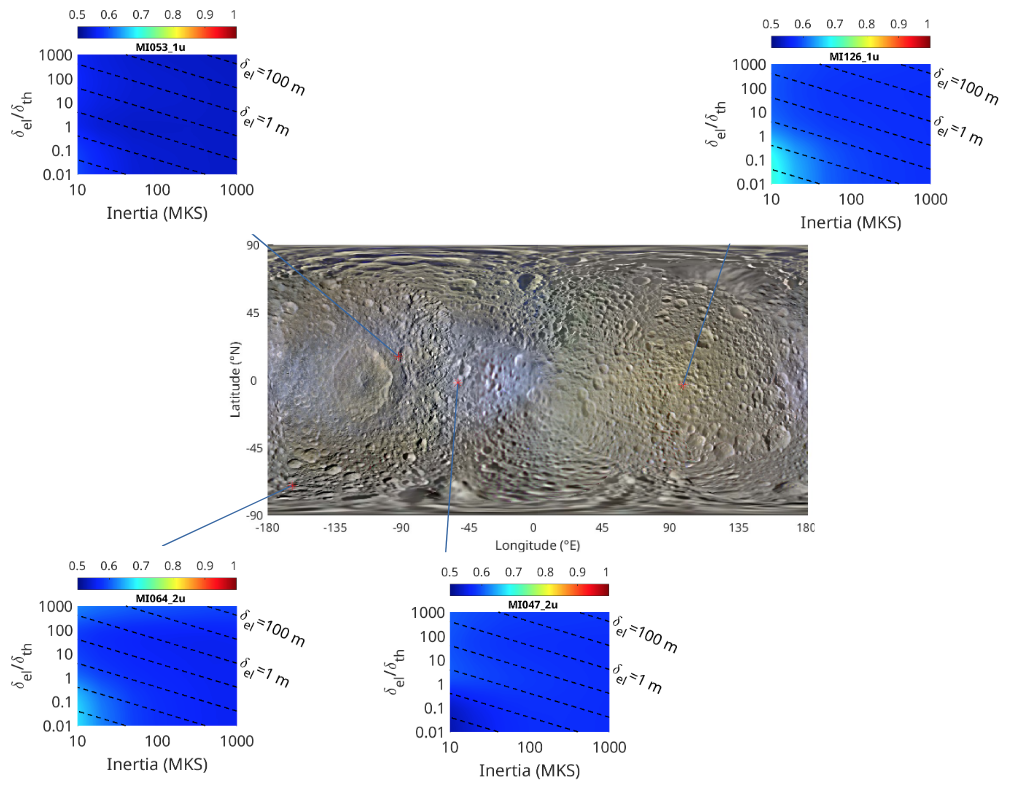
Fig. 1: 2.2-cm emissivity of Mimas’s surface derived from Cassini distant radiometry observations and a combined thermal and radiative transfer model as a function of Mimas subsurface thermal and electrical properties (namely its thermal inertia and the ratio of its electrical and thermal skin depths). The sub-spacecraft point of each distant observation is indicated on an ISS map of the satellite.
How to cite: Le Gall, A., Sultana, R., Bonnefoy, L., Leyrat, C., and Janssen, M. A.: Microwaving Saturn's airless icy moons Mimas, Enceladus, Tethys, Dione, Rhea, Iapetus and Phoebe, Europlanet Science Congress 2022, Granada, Spain, 18–23 Sep 2022, EPSC2022-607, https://doi.org/10.5194/epsc2022-607, 2022.
Ganymede’s water exosphere has been observed spectroscopically on several occasions since the first detection of atomic hydrogen in Ganymede’s exosphere in 1997 [1]. From these observations a consistent picture of Ganymede’s exosphere has emerged: Ganymede’s day-side exosphere is dominated by sublimated water with inferred column densities of up to several 1e15 cm-2, while elsewhere the exosphere is dominated by sputtered molecular oxygen (inferred column densities of several 1e14 cm-2) at low altitudes and by atomic oxygen (inferred column densities of several 1e13 cm-2) at higher altitudes [2-9]. In addition, atomic hydrogen has been observed with inferred column densities of a few 1e12 cm-2 [1, 4, 10]. Whereas many modeling approaches have been able to reproduce the inferred H2O and O2 densities, they have struggled to re-create the high inferred atomic oxygen and hydrogen column densities [11-13].
In this work, we present new simulations of Ganymede’s water-related exosphere. Our modeling results reproduce the observed H2O emissions well by sublimating water at Ganymede’s day-side surface temperature. The observed OI emission lines, which were interpreted as an O2 atmosphere, on the other hand, agree with a sputter source, with Jupiter’s magnetospheric plasma acting as the sputter agent.
Ganymede has a complex magnetic field, that shields part of the surface (mainly the equatorial regions) from impinging plasma ions and electrons, leaves the polar caps exposed to unhindered plasma precipitation, and accelerates the precipitating plasma in the separatrix, resulting in strong auroral emissions [2-8]. We show that the thermal electrons reaching the polar caps are insufficient to produce the amount of atomic oxygen and hydrogen inferred from the observations, and that an interaction between the water atmosphere and auroral electrons is necessary. In addition, we will discuss how the Particle Environment Package [14] onboard ESA’s JUpiter and ICy moons Explorer [15] will help us learn more about Ganymede’s atmosphere and plasma environment.
[1] Barth, C. A., C. W. Hord, A. I. F. Stewart, W. R. Pryor, K. E. Simmons, W. E. McClintock, J. M. Ajello, K. L. Naviaux, and J. J. Aiello (1997), “Galileo ultraviolet spectrometer observations of atomic hydrogen in the atmosphere of Ganymede”, Geophysical Research Letter, 24(17), 2147–2150.
[2] Hall, D. T., P. D. Feldman, M. A. McGrath, and D. F. Strobel (1998), “The Far-Ultraviolet Oxygen Airglow of Europa and Ganymede”, The Astrophysica Journal, 499(1), 475–481.
[3] Brown, M. E., and A. H. Bouchez (1999), “Observations of Ganymede’s visible aurorae”., in Bulletin of the American Astronomical Society, vol. 31.
[4] Feldman, P. D., M. A. McGrath, D. F. Strobel, H. W. Moos, K. D. Retherford, and B. C. Wolven (2000), “HST/STIS Ultraviolet Imaging of Polar Aurora on Ganymede”, The Astrophysical Journal, 535(2).
[5] McGrath, M. A., X. Jia, K. Retherford, P. D. Feldman, D. F. Strobel, and J. Saur (2013), “Aurora on Ganymede”, Journal of Geophysical Research (Space Physics), 118(5), 2043–2054.
[6] Saur, J., S. Duling, L. Roth, X. Jia, D. F. Strobel, P. D. Feldman, U. R. Christensen, K. D. Retherford, M. A. McGrath, F. Musacchio, A. Wennmacher, F. M. Neubauer, S. Simon, and O. Hartkorn (2015), “The search for a subsurface ocean in Ganymede with Hubble Space Telescope observations of its auroral ovals”, Journal of Geophysical Research (Space Physics), 120(3).
[7] Musacchio, F., J. Saur, L. Roth, K. D. Retherford, M. A. McGrath, P. D. Feldman, and D. F. Strobel (2017), “Morphology of Ganymede’s FUV auroral ovals”, Journal of Geophysical Research (Space Physics), 122(3).
[8] Molyneux, P. M., J. D. Nichols, N. P. Bannister, E. J. Bunce, J. T. Clarke, S. W. H. Cowley, J. C. Gérard, D. Grodent, S. E. Milan, and C. Paty (2018), “Hubble Space Telescope Observations of Variations in Ganymede’s Oxygen Atmosphere and Aurora”, Journal of Geophysical Research (Space Physics), 123(5).
[9] Roth, L., N. Ivchenko, G. R. Gladstone, J. Saur, D. Grodent, B. Bonfond, P. M. Molyneux, and K. D. Retherford (2021), “Evidence for a sublimated water atmosphere on Ganymede from Hubble Space Telescope observations”, Nature Astronomy, 5.
[10] Alday, J., L. Roth, N. Ivchenko, K. D. Retherford, T. M. Becker, P. Molyneux, and J. Saur (2017), “New constraints on Ganymede’s hydrogen corona: Analysis of Lyman-α emissions observed by HST/STIS between 1998 and 2014”, Planetary and Space Science, 148.
[11] Marconi, M. (2007), A kinetic model of ganymede’s atmosphere, Icarus, 190(1).
[12] Turc, L., L. Leclercq, F. Leblanc, R. Modolo, and J.-Y. Chaufray (2014), Modelling ganymede’s neutral environment: A 3d test-particle simulation, Icarus, 229.
[13] Leblanc, F., A. Oza, L. Leclercq, C. Schmidt, T. Cassidy, R. Modolo, J. Chaufray, and R. Johnson (2017), On the orbital variability of ganymede’s atmosphere, Icarus, 293.
[14] Barabash, S., Wurz, P., Brandt, P., Wieser, M., Holmström, M., Futaana, Y., et al. (2013). “Particle Environment Package (PEP)”, European Planetary Science Congress 2013.
[15] Grasset, O., Dougherty, M. K., Coustenis, A., Bunce, E. J., Erd, C., Titov, D., et al. (2013). “JUpiter ICy moons Explorer (JUICE): An ESA mission to orbit Ganymede and to characterise the Jupiter system”. Planetary and Space Science, 78, 1–21.
How to cite: Vorburger, A., Fatemi, S., Galli, A., Carberry Mogan, S., Roth, L., and Wurz, P.: 3D Monte-Carlo Simulation of Ganymede’s Water-Related Exosphere, Europlanet Science Congress 2022, Granada, Spain, 18–23 Sep 2022, EPSC2022-635, https://doi.org/10.5194/epsc2022-635, 2022.
- 1. Introduction
Tethys is unusual among icy moons for its low bulk mean density of 0.985 g/cm3, suggesting a low rock mass fraction and/or high porosity. Like other mid-sized icy satellites Tethys has an intense fracture history [1], including Ithaca Chasma as well as several hundred arcuate andlinear troughs, grooves, and cracks. Unique to Tethys, however, are dark reddish linear features visible to Cassini under high solar illumination conditions (a lower albedo and flatter spectral signature in the green–IR range; Figs. 1, 2). Our CDAP-funded research is focused on mapping these features and testing hypotheses for their formation and implications for Tethys’ evolution

Figure 1: Color view of Tethys showing IR lineations (reddish arcs). Cassini IR3, green, UV3 image composite.

Figure 2: Preliminary spectral plot showing IR lineaments (red) and adjacent cratered plains (green) from ISS images.
Figure 3: Global map of fractures, ridges, and lineations on Tethys. IR lineations are shown in red. Odysseus is large circle at upper center.
1.1 IR-Lineations
There are at least three prominent sets in the northern anti-Saturn hemisphere, centered on the anti-Saturn meridian (Fig. 3). Each setconsists of ~5–10 parallel lineations a few kilometers across and 50–250 km long. The lineations are remarkably curvilinear (i.e., non-sinuous), do not follow great circles, and are not deflected by major impact structures: they cross the floor of the 400-km-diameter, 9-km-deep Odysseus impact basin as if it were not there.
Although more poorly observed, sub-Saturn hemispheric color imaging at low-phase angle clearly shows a similar set of arcuate, reddishlineations on that hemisphere, despite deposition of E-ring dust particles from Enceladus [2] indicating that these features are being renewed on some time-scale.
The red lineaments centered near ~25° N, 175°E were imaged at high resolution. Mapping at ~90–125 m/pixel (Fig. 4) (together with stereo andlower resolution color imaging) shows no discrete scarp, ridge, or other tectonic manifestation along the ~100 km portion of the feature soimaged. Only a faint discoloration of the surface has been identified (Fig. 5). Further, >20 dark spots 200–800 m in diameter lie along this setof lineaments. These spots are characterized by very low albedos, sharp boundaries, and no evidence of raised rims consistent with an impactorigin. Of these, >60% are situated at the bottom of impact craters.

Figure 4: High-resolution, 90 m/pixel mosaic of IR lineaments, merged with IR3–Gr–UV3 color mosaic.

Figure 5: Enlargement of high-resolution view in Figure 4 showing reddish lineament (red arrows) and small dark spots (blue arrows).
Red streaks centered at 45° N, 333°E were targeted for high resolution ISS and VIMS observations in late 2015 (although the VIMS cubes were partially corrupted). As at the above site no discrete faults, scarps or grooves was resolved here despite pixel scales as good as ~60 m.
- 2. Origin of IR-Lineaments
The spatial pattern of IR lineaments on Tethys shows a strong symmetry (Fig. 3), centered on the current tidal axis with Saturn. A lack ofcorrelation with local geology might suggest an exogenic origin. Conversely, there are no rayed craters at the radial centers of these features.Further, the locations of the patterns on both the sub- and anti-Saturn hemispheres, and the lineaments’ parallel orientations, argue against adisrupted comet origin (à la SL9). The lineaments have no systematic orientation relative to Odysseus, indicating that stresses arising fromthe relaxation of that basin [3] are not responsible for these features.
Global stresses might have produced the pattern we observe. The IR lineaments may match patterns of strain predicted to result from a non-synchronous rotation stress state, although this is unlikely for a cold, triaxial body like Tethys. The best-fit patterns correspond to a combination of global expansion with true polar wander or tidal axis reorientation (Fig. 6a, b). The misfit for global expansion combined recession is significantly larger (Fig. 6c). The dramatic lack of such features in the southern hemisphere (Fig. 3), where only a few short isolated red streaks are evident, is not explained by any currently considered stress regime.
Figure 6: (a-c) Observed (red) and predicted (green) tectonic patterns due to combination of global expansion with (a) true polar wander, (b) tidal axis reorientation, (c) orbit recession. Solid and open circles indicate location of initial rotation and tidal axes. (d) Relative frequency distribution of misfit between observed and predicted fault segment azimuths for processes in panels a-c. Labels show mean misfit for each model.
The lack of obvious tectonic deformation despite the strong color signature is unusual (although features may exist below the currentresolution limit). The lineaments could be reactivated ancient fractures, producing a temporal discoloration. At present there is no topographic or morphologic signature to support this. If tectonic, the lineaments might be still forming, with deformation only on a scale below that which we can resolve.
The dark and reddish coloration could be due to a particulate contaminant in the ice grains that is more spectrally visible if the grain sizes are larger along the streaks. Alternatively, a dark reddish contaminant has been deposited on the surface along the streaks. Such a contaminant could be due to precipitation of a distinct material along unresolved surface or near-surface fractures, with subsequent mixing of contaminant into the local regolith. VIMS spectral cubes are being reprocessed to verify whether organic rich materials may be involved. Low-volume but persistentoutgassing and emplacement of volatiles from the interior (possibly due to clathrate decomposition associated with fracture formation) thecolors of which are distinct from the evolved surface and/or result from alteration due to exposure to the space environment, may be responsible.
The coloration of Tethys unique red streaks, and collocated dark spots, are consistent with active alteration of the surface, given that E-ringaccumulation is expected to remove intrinsic color signatures in a geologically short time period. Differences in particle sizes of the outgassed material may add to this spectral distinctiveness.
How to cite: Schenk, P., Buratti, B., Clark, R., Byrne, P., McKinnon, W., Matsuyama, I., Nimmo, F., and Scipioni, F.: Red Streaks on Tethys: Evidence for Recent Activity, Europlanet Science Congress 2022, Granada, Spain, 18–23 Sep 2022, EPSC2022-732, https://doi.org/10.5194/epsc2022-732, 2022.
Io is the innermost galilean satellite of Jupiter and object to extreme tidal forces. As a result of these forces Io is the most volcanically active body in our solar system. Its large volcanic plumes can rise up to several hundred kilometres above the surface and are one known source of Io's SO2 atmosphere. Additionally, the surface of the moon is covered with surface frost which sublimates in sunlight and condenses during the night or when Io enters eclipse behind Jupiter. Therefore, Io’s atmosphere is a result of the combination of volcanism and sublimation, but it is unknown exactly how these processes work together to create the observed atmosphere. That is why we want to present an approach on modelling Io’s atmosphere and provide a better understanding of the ongoing dynamic processes.
Both, the gas flow of the plume and the sublimation atmosphere, are modelled using the Direct Simulation Monte Carlo (DSMC) method first utilised by G. A. Bird [1]. The DSMC method is the most suitable for this case because the gas dynamics can be modelled over a great range of gas densities which is especially important for rarefied gas flows at high altitudes and on the night side of Io. It is a particle-based method which returns a 3D gas flow field as a result. While we currently focus on single species simulations, our DSMC code is designed to support multiple species enabling us to study the gas emission of other volcanic features as for example lava lakes in the future. This allows us to investigate the influence and contributions of different processes to the atmosphere. The idea of our work is based on simulations done by McDoniel et al. [2].
In a first case, we are investigating the flow of SO2 gas from the source of a plume, into the umbrella-shaped canopy and eventually back onto the surface locally. Additionally, we also study the interaction of the plume with an ambient sublimation atmosphere. In a second case, data obtained by the Galileo SSI experiment is used to create a surface albedo map of Io which enables us to calculate a more precise global thermal model for the sublimation atmosphere. We can then place plumes on the surface and study the interaction of volcanic and sublimation effects globally. Finally, we are also able to implement dust particles in the plume and analyse the effect for different dust sizes. From these results we can calculate images of the column density and the reflectance which in a next step could be used to compare to observational data.
Overall, our goal is to gain a better understanding of the plume structure, the interaction with the ambient atmosphere and the overall contribution of different processes to Io's atmosphere in preparation for future missions such as JUICE, Europa Clipper and a possible future Io Volcano Observer.
[1] Bird, G. A. (1994). Molecular Gas Dynamics and the Direct Simulation of Gas Flows.
[2] McDoniel, W. et al. (2019). Simulation of Io’s plumes and Jupiter’s plasma torus. Phys. Fluids 31, 077103. DOI: 10.1063/1.5097961.
How to cite: Klaiber, L., Thomas, N., Marschall, R., and Milazzo, M.: DSMC Simulations of Io’s atmosphere, Europlanet Science Congress 2022, Granada, Spain, 18–23 Sep 2022, EPSC2022-931, https://doi.org/10.5194/epsc2022-931, 2022.
OPS6 | Aerosols and clouds in planetary atmospheres
Abstract
We present Doppler wind velocity final results of Saturn’s zonal flow at cloud level. Our aim is help to constrain the characterization of the equatorial jet at cloud level and the latitudinal variation of the zonal winds, to measure its spatial and temporal variability, to contribute to monitor the variability in order to achieve a better understanding of the dynamics of Saturn’s zonal winds (Sánchez-Lavega et al. 2003, 2007, 2016); Finally, the complementarity with Cassini, providing an independent set of observations.
Figure 1: (a) Raw echellogramme showing the spectral orders for one of the detectors. (b) Magnification of part of one order, where absorption lines (dark vertical bands) are visible. From each order, a stack of 61 spectra are extracted. (c) Set of 61 spectra, with each one corresponding to one pixel in the slit’s active window. (d) Each spectrum is divided into 16 orders in the MIT detector and 23 orders in the EEV detector. The plot shows an example of the 16 components of an MIT spectrum, each coming from one spectral order. (e) Example spectrum from one order and one location in the Venus disk. Machado et al. (2012).
The study of the planet’s global system of winds at the 0.7 bar region is based on high resolution spectra from the UV-Visual Echelle Spectrograph (UVES) instrument at ESO’s Very Large Telescope (VLT). Under the assumption of predominantly zonal flow, this method allows the simultaneous direct measurement of the zonal velocity across a range of latitudes and local times. The technique, based on long slit spectroscopy combined with the high spatial resolution provided by the VLT, has provided the first ground-based characterization of the latitudinal profile of zonal wind in the atmosphere of Saturn and the first zonal wind field map in the visible. It promises to improve the characterization of the equatorial jet and the latitudinal variation of the zonal winds, as well the measurement (and monitorization) of its spatial and temporal variability, achieving a better understanding of the dynamics of Saturn’s zonal winds (which Sánchez-Lavega have found to have changed in recent years). A complete characterization of the dynamical behaviour of Saturn atmosphere is crucial for understanding its driving mechanisms. Finally, the complementarity with Cassini, has provided an independent set of observations to compare with and help validate the method. The zonal wind profile retrieved is consistent with previous spacecraft measurements based on cloud tracking, but with non-negligible variability in local time (longitude) and in latitude.
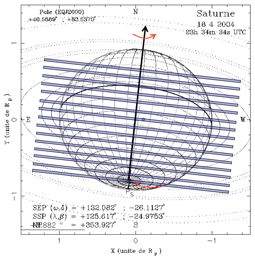
Figure 2: Geometry of the slit positions at the observation days. Saturn’s diameter is 17.4", and the slit aperture is 0,3”x25” . The aperture offset between consecutive exposures is 1". The sub-terrestrial point is at -26.1ºS.
The UVES/VLT instrument has been used, which simultaneously achieves high spectral resolving power and high spatial resolution. The field has been derotated in order to have the aperture aligned perpendicularly to Saturn’s rotation axis. In this configuration, spatial information in the East-West direction is preserved in a set of spectra in the direction perpendicular to dispersion. Our Doppler velocimetry method is based on the technique of absolute accelerometry (Connes, 1985) which has been applied to the backscattered solar spectrum in order to determine the Doppler shift associated with the zonal circulation. Our measurements have been made in the wavelength range of 480-680 nm. Previously we successfully adapted and fine tuned this Doppler velocimetry technique for measuring winds at Venus cloud tops (Machado et al. 2012, 2014,2017, 2021; Gonçalves et al., 2020). In the present study we will show the adaptation of this method for Saturn’s case. We will use coordinated observations from the Cassini’s Visible and Infrared Mapping Spectrometer (VIMS), in order to compare with the Doppler winds obtained from the UVES/VLT high-resolution spectra.
The observations consisted of 4 blocks of 15 exposures of 90 sec, plus two shorter blocks of 9 exposures, totaling 7.3 hours of telescope time. In order to cover the whole disk the aperture has been offset by 1 arcsec in the North-South direction between consecutive exposures. Most of the northern hemisphere was covered by the rings. Saturn’s diameter was 17.4 arcsec, and the slit aperture was 0.3x25 arcsec. The aperture offset between consecutive exposures was 1 arcsec. Two shorter observations blocks of 9 exposures only covered the central part of the disk, and four others covered the whole disk. The sub-terrestrial point was at -26.1 S. The presence of the rings lead to severe order superposition. The dark region between the rings and the disk may or may not be present, depending on the slit position. On the other hand, defects in the response of the UVES slit in the upper part preclude its use for accurate Doppler measurements such as these. For these reasons only the central part of the aperture has been considered for the measurements.
It can be easily noticed that we were able to reproduce with a significant agreement the amplitudes of the wind velocities previously observed in a vast range of latitudes and that they are highly consistent with the cloud tracking measurements from almost simultaneous Cassini data.
Figure 3: Contour map of Saturn disk for the first night of observations. The wind velocities have units of m/s. Thecolor scale was arbitrary.
References
Connes, P., Absolute Astronomical Accelerometry, Astrophysics and Space Science (ISSN 0004-640X), volume 110, no. 2, p.211-255, 1985.
Goncalves, R., Machado, et al., Icarus, 335, article id. 113418, 2020.
Machado, P., Luz, D.Widemann, T., Lellouch, E.,Witasse, O, , Icarus, Volume 221, p. 248-261, 2012.
Machado, P., Widemann, T., Luz, D., Peralta, J., Icarus, 2014.
Machado, P., Widemann, T., Peralta, J., Gonçalves, R., Donati, J-F., Luz, D., Icarus, 285, 8-26, 2017
Machado, P., et al., Atmosphere, 12, 506, 2021.
Sánchez-Lavega, A., et al., Nature, 423, 623-625, 2003.
Sánchez-Lavega, A., Hueso, R.; Pérez-Hoyos, S., Icarus, 187, 510-519, 2007.
Sánchez-Lavega, A., et al., Nature Communications, 7, id. 13262, 2016.
How to cite: Machado, P., Silva, M., Sánchez-Lavega, A., Silva, J., Espadinha, D., Brasil, F., and Ribeiro, J.: Saturn atmosphere's winds with VLT/UVES Doppler velocimetry, Europlanet Science Congress 2022, Granada, Spain, 18–23 Sep 2022, EPSC2022-354, https://doi.org/10.5194/epsc2022-354, 2022.
Titan’s atmosphere includes many trace hydrocarbon and nitrile species that reach their condensation temperatures in the stratosphere. These, for the most part, will condense out as ices given sufficient condensation nuclei, which are provided by the organic haze particles. Barth (2017) explored the physics behind the size and abundance of pure ice particles that could be present in Titan’s atmosphere and found they would condense out in layers between about 80 and 60 km given thermal conditions at the Huygens landing site (Fig. 1).
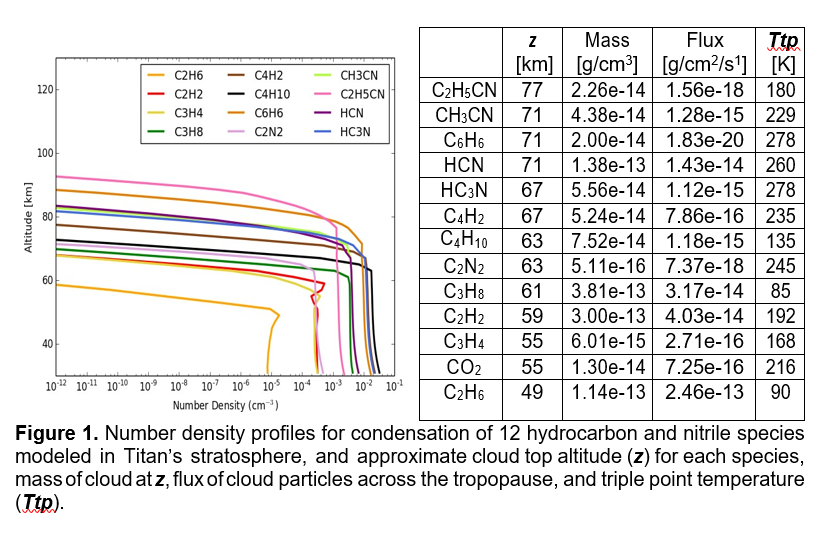
We now expand that study to multiple latitudes and include mixtures of trace species in the ice particles. Anderson et al. (2018) have shown that in Titan’s stratosphere, where many of the trace gases are saturated at the same altitude, they are likely co-condensing onto the haze particles. This changes the optical properties of the particles, but microphysically the formation process is similar to modeling the pure ices, as long as the vapor pressures are adjusted for the mixture.
Modeling is done using the Community and Aerosol Radiation Model for Atmospheres (CARMA; Barth 2020). CARMA models the physics of vertical transport and coagulation in a column of atmosphere and the interaction of particles and gases through nucleation, condensation, and evaporation. The growth routines have been modified to include particles composed of multiple volatiles, with each volatile component growing or evaporating in response to the environment (Barth & Toon, 2006). Particles are represented by a number of discrete mass bins, such that the size distribution of ice particles can be explored at all altitudes in the column. The model keeps track of the changes with time of the number of particles (including core mass for clouds) and mass density of volatiles.
This work is supported by NASA CDAP 80NSSC20K0485.
References: Anderson, C. M., R. E. Samuelson and D. Nna-Mvondo 2018. Organic ices in Titan’s stratosphere. Space Sci. Rev. 214, 125; Barth, E.L. 2020. PlanetCARMA: A New Framework for Studying Planetary Atmospheres. Atmosphere, 11(10), 1064; Barth, E. L. 2017. Modeling survey of ices in Titan’s stratosphere. Planet. Space Sci. 137, 20–31; Barth, E. L., and O. B. Toon 2006. Methane, ethane, and mixed clouds in Titan’s atmosphere: Properties derived from microphysical modeling. Icarus 182, 230–250.
How to cite: Barth, E. L.: Microphysical modeling of mixed composition ices in Titan’s stratosphere, Europlanet Science Congress 2022, Granada, Spain, 18–23 Sep 2022, EPSC2022-765, https://doi.org/10.5194/epsc2022-765, 2022.
We have determined the real and imaginary refractive indices (n and k, respectively), from the visible to the near infrared (0.4 to 1.6 µm), of five laboratory-generated organic refractory materials produced from gas-phase chemistry with the NASA Ames COSmIC facility. The solid samples were produced using a plasma discharge in the stream of a 200-K supersonic jet-cooled expansion of different gas mixtures to study the impact of the molecular precursors on the solid sample optical properties. Three samples were produced from N2:CH4 (95:5) gas mixtures using three different high voltages (700V, 800V and 1000V) to vary the energy in the plasma discharge. One sample was produced from a N2:CH4:C2H2 (94:5:5:0.5) gas mixture, with a high voltage of 1000 V. The fifth sample was produced in an Ar:CH4 (95:5) gas mixture with a high voltage of 1000 V to produce a nitrogen-free hydrocarbon sample. The optical constants, n and k, of these five samples were determined using spectral reflectance measurements. They appear to be positively correlated with the nitrogen content in the solid sample, i.e., a sample with larger nitrogen content exhibits higher n and k values.
We have used these refractive indices as input parameters in a radiative transfer model to analyze Cassini Visible Infrared Mapping Spectrometer (VIMS) observations of Titan’s atmosphere. The results show that using the tholin samples with higher n and k values (higher nitrogen content) provides a better fit to the observational data than using the samples with lower n and k values (lower nitrogen content). The Titan tholins with higher nitrogen content therefore appear to be more representative of the Titan aerosols observed by VIMS.
How to cite: Sciamma-O'Brien, E., Roush, T., Rannou, P., and Salama, F.: First Optical Constants from 0.4 to 1.6 µm of Titan Aerosol Analogs Produced in the NASA Ames COSmIC Facility and Their Use in a New Analysis of Cassini VIMS Observations, Europlanet Science Congress 2022, Granada, Spain, 18–23 Sep 2022, EPSC2022-1199, https://doi.org/10.5194/epsc2022-1199, 2022.