Abstracts with displays
TP1 | Mercury Science and Exploration
The discrete photoemission properties of atomic and molecular species stimulated by solar radiation are an important tool for quantitative work with remote sensing experiments. In an optically thin atmosphere, the total column amount of a given species is given in terms of a solar-forced g-value, defined as an emission probability per atom (photon s−1atom−1). For an optically thin gas and a measured emission brightness (4πI), the column abundance N is obtained through the relation 4πI= gN. Discrete emission lines and Fraunhofer features in the solar spectrum are responsible for a strong dependence of the g-values on Doppler velocity for many species. Because of Mercury’s eccentric orbit, some g-values can vary by over an order of magnitude during the orbital period. In addition, g-values are dependent on the instantaneous heliocentric radial velocity, which varies as an atom is ejected from the surface and moves through gravitational and radiation pressure accelerations. Thus knowledge of how the g-values vary is critical to interpretation of spectroscopic data. In previous work, g-values were calculated for 12 species that were to be targeted by MESSENGER. The species of interest included sodium, potassium, and calcium, which had been observed in Mercury’s exosphere through ground-based observations pre-MESSENGER, and hydrogen and oxygen, measured (or potentially only an upper limit in the case of O) by the UV spectrometer experiment on the Mariner 10 spacecraft. In addition, sulfur, magnesium, carbon, Ca+ and Mg+ are observable by Bepi-Colombo as well as MESSENGER. Helium EUV emission at 584 Å, not within the MESSENGER UVVS wavelength range, will be observable with the Bepi-Colombo UV spectrometer. Of particular importance for Mercury is the dependence of the g-values on the bulk motion of the gas relative to the Sun. This heliocentric relative velocity is often quite large due to the high initial velocity of the ejected atoms and the subsequent radiation pressure acceleration.
- Motivation
Mercury’s orbit is highly elliptical, having an ellipticity of 0.2. This results in a variation of the heliospheric relative velocity varying by ± 10 km/s. The g-values published by Killen et al. (2009) were therefore calculated for Doppler shifts of this magnitude. However, it has become apparent that the heliocentric relative velocity of atoms in Mercury’s exosphere varies considerably more than the velocity at rest with respect to the planet, both due to the initial ejection velocity and due to radiation pressure, that is especially strong for Na. The velocity of Ca atoms is also extreme, due to as yet unknown processes, but possibly due to dissociation of a Ca-bearing molecule. We have therefore extended the g-values to ±50 km/s relative to their at-rest values. The g-values have been scaled using the solar spectrum originally used by Killen et al. (2009) (e.g. Hall and Anderson, 1991) and available in the appendix to that paper. In addition, for the Mg line at 285.296 nm, we used the TSIS-1 solar spectrum available from the LISIRD website (https://lasp.colorado.edu/lisird/). In March 2022, the TSIS-1 HSRS was recommended as the new solar irradiance reference spectrum by the Committee on Earth Observation Satellites (CEOS) Working Group on Calibration and Validation (WGCV). TSIS-1 HSRS is developed by applying a modified spectral ratio method to normalize very high spectral resolution solar line data to the absolute irradiance scale of the TSIS-1 Spectral Irradiance Monitor (SIM) and the cubesat Compact SIM (CSIM). The spectral resolution of this spectrum is 0.25 nm. The high spectral resolution solar line data from the Air Force Geophysical Laboratory ultraviolet solar irradiance balloon observations, used in the Killen et al. (2009) work, have a spectral resolution of 0.015 nm. The g-values calculated herein at high resolution must be convolved to the spectral resolution of the instrument used for the observations to be analyzed. The UVVS spectrometer on MESSENGER was a scanning grating monochromator that covered the wavelength range 1150 - 6100 Å with an average 6 Å spectral resolution (McClintock & Lanton 2007). The Bepi Colombo UV spectrometer, PHEBUS, is a double spectrometer for the Extreme Ultraviolet range (550 - 1550 Å) and the Far Ultraviolet range (1450 - 3150 Å) using two micro-channel plate (MCP) detectors with spectral resolution of 10 Å for the EUV range and 15 Å for the FUV range (Chassefiere et al. 2008).
We show plots of extended g-values for Na (D1), K (D1 & D2), Ca, and Mg. The Mg g-values are given for both the Hall and Anderson (1991) solar spectrum and for the TSIS-1 spectrum for comparison of high and low-resolution results.

Figure 1. The g-value for Na (D1) at 589.756 nm in vacuum continues to increase as the Doppler shift increases. The D2 line g-values similarly increase beyond a velocity of ±10 km/s to ± 50 km/s. Therefore the column abundance for high velocity atoms will be over-estimated using the formerly published g-values. This is especially important for estimates of escape.

Figure 2. G-values for the Ca 422.7 nm line calculated to ±50 km/s. In the case of the Ca line, the g-value continues to increase for heliocentric relative velocity > 25 km/s, but decreases for heliocentric relative velocities < -35 km/s. As for Na, the Ca column abundance anti-sunward of Mercury will be overestimated using the previously published g-values.

Figure 3. The extended g-values for the K (D2) line at 404.53 nm (green) and K (D1) 404.84 nm (vacuum wavelengths) at 0.352 AU are quite complex owing to the underlying solar spectrum. Care must be taken to calculate the column abundance at the instantaneous heliocentric relative velocity of the atom.

Figure 4. The g-value for the Mg 285.296 nm line is also quite complex. This figure shows the g-value calculated using the high resolution of the Hall and Anderson (1991) solar spectrum at a spectral resolution of 15 mÅ.

Figure 5. The g-value for the Mg 285.296 nm line using the low resolution TSIS-1 spectrum at 0.25 Å resolution shows little high frequency variation, as expected.
How to cite: Killen, R., Vervack, R., and Burger, M.: Variation of g-values of major species with heliocentric velocity, Europlanet Science Congress 2022, Granada, Spain, 18–23 Sep 2022, EPSC2022-53, https://doi.org/10.5194/epsc2022-53, 2022.
In this work, we apply a method previously discussed in [1] to assess the presence of water ice in Mercury’s Polar Shadowed Regions (PSR) mixed to S-rich volatile species like SO2, H2S, and volatile organics, intending to verify their detectability from Bepi Colombo’s orbit and to optimize SIMBIO-SYS/VIHI observations. PSR icy deposits located within the floor of the Kandinsky crater are simulated in terms of I/F spectra corresponding to mixtures of H2O-H2S and H2O-SO2 with grain sizes of 10, 100, and 1000 µm as resulting from indirect illumination by the scattered solar light coming from the crater’s rim. The spectral simulations, performed following the method described in [2], and including the ice-regolith mixing (areal or intimate) as modeled in [3], allow for exploring different volatile species abundances and grain size distribution.
The resulting ice detection threshold are evaluated by means of the computation of VIHI’s instrumental signal-to-noise ratio as given by the instrumental radiometric model [4]. In this way, a synergistic use of illumination models, spectral simulations and resulting SNR calculations will help us to optimize the VIHI’s observation strategy across Mercury’s polar regions with the aim to detect, identify and map volatile species. This task is one of the primary scientific goals of the 0.4-2.0 µm Visible and Infrared Hyperspectral Imager (VIHI) [5], one of the three optical channels of the SIMBIO-SYS experiment [6] on ESA’s BepiColombo mission.
Due to orbital characteristics and proximity to the Sun, Mercury’s polar regions undergo large variations in illumination conditions during the hermean year [1]. At poles, Permanent Shadowed Regions (PSRs) occur on deep craters and rough morphology terrains that are not directly illuminated by the Sun during the hermean day. Nevertheless, some of these areas could experience partial illumination caused by multiple scattered light coming from nearby illuminated areas. Despite the orbital vicinity to the Sun, Mercury’s PSRs can maintain cryogenic temperatures across geological timescales resulting in the condensation and accumulation of volatile species [7]. While water ice is the more certain species in Mercury’s PSR, it is not precluded the occurrence of other secondary species rich in sulfur or even organic matter.
In fact, the total surface area of PSRs between latitudes 80−90° south is not negligible, being estimated at about 25.000 km2 [8], about two times larger than the same geographic area on the North Pole [9].
References: [1] Filacchione G. et al., MNRAS, 498, 1308-1318, 2020. [2] Raponi A. et al., Sci. Adv., 4, eaao3757, 2018. [3] Ciarniello. M. et al., Icarus, 214, 541, 2011. [4] Filacchione G. et al., Rev. Sci. Instrum., 88, 094502, 2017. [5] Capaccioni F. et al., IEEE Trans. Geosci. Remote Sens., 48, 3932, 2010. [6] Cremonese G. et al., Space Sci. Rev., 216, 75, 2020. [7] Paige D. A. et al., Science, 339, 300, 2013. [8] Chabot N. L. et al., J. Geophys. Res., 123, 666, 2018. [9] Deutsch A. N. et al., Icarus, 280, 158, 2016.
Acknowledgments: We gratefully acknowledge funding from the Italian Space Agency (ASI) under ASI-INAF agreement 2017- 47-H.0.
How to cite: Filacchione, G., Raponi, A., Ciarniello, M., Capaccioni, F., Frigeri, A., Galiano, A., De Sanctis, M. C., Formisano, M., Galluzzi, V., and Cremonese, G.: DETECTION OF ICY SPECIES IN MERCURY’S PSRs: SPECTRAL SIMULATIONS FOR SIMBIO-SYS/VIHI ON BEPI COLOMBO, Europlanet Science Congress 2022, Granada, Spain, 18–23 Sep 2022, EPSC2022-191, https://doi.org/10.5194/epsc2022-191, 2022.
Strofio is a mass spectrometer, aboard the BepiColombo mission, that utilizes a time-of-flight method to determine the mass-per-charge of each particle entering its aperture in order to study the chemical composition of the exosphere of Mercury. Optimization of Strofio involves finding a balance between system efficiency and mass resolution while increasing the signal-to-noise ratio. In order to ensure our data is exospheric in nature, we must separate the Mercury environment from the background environment. The background environment is made up of thermal particles produced from sources like the outgassing of the spacecraft as well as from the instrument itself. This problem can be addressed by assigning the correct voltages to the source apparatus, thereby realizing a background filter. This filter works best in Mach 2 or larger regimes to ensure the targeted particles do not get filtered out with the background. My work focuses on writing and running a series of computer simulations that optimize the velocity filter in accordance with the configuration of the flight model.
How to cite: Schroeder, J., Livi, S., Allegrini, F., and Wurz, P.: Increasing the Signal-to-Noise Ratio of a Mass Spectrometer Using a Velocity Filter, Europlanet Science Congress 2022, Granada, Spain, 18–23 Sep 2022, EPSC2022-368, https://doi.org/10.5194/epsc2022-368, 2022.
Mercury possesses the second, highest density (5.23 g/cm3) in the Solar System after Earth. This high density is likely the result of the presence of a large inner core, composed of iron-light elemental alloys, overlayed by a relatively thin silicate shell, comprising the crust and the mantle [1]. The mercurian crust has been analyzed by the Messenger spectroscopic suite of instruments, which included, among others, the XRS (X-ray Spectrometer) and GRS (Gamma-Ray Spectrometer) spectrometers, capable of detecting the elements present on Mercury’s surface. The surface mineralogy of Mercury is dominated by enstatite and plagioclase, with small amounts of sulfides (oldhamite, CaS), the presence of which is a strong clue of the extremely reducing conditions which have led to Mercury’s accretion and differentiation [2]. The mercurian crust has been found to be very thin with estimates ranging between 26 ± 11 km and 35 ± 18 km [3,4]. Moreover, the mercurian mantle is also thin, thinner than other terrestrial planets' mantles, with an estimated thickness between 300 km – 500 km [5]. In addition, the mantle shows a great lateral heterogeneity in mineral compositions, as indicated by the local, abrupt chemical changes in crustal chemistry [6].
Mercury’s large metallic core, likely partially molten and making up to 42% of its volume, combined with surficial observations (which have revealed a very small FeO concentration), and the peculiar position occupied by Mercury in the solar nebula, lead us to hypothesize a very reduced geochemical environment as its birthplace [7]. In literature, chondrites belonging to CB and enstatite chondrites (EN) have been considered the best precursor materials for Mercury’s composition [6, 8, 9, 10], sharing many analogies both in geochemistry and thermal evolution.
In light of the above, we chose a CB-like bulk composition to model the mineral assemblage of the mercurian mantle.
We reconstruct the evolution of the mercurian mantle starting from a CB chondrite-like bulk silicate composition, at thermodynamic equilibrium, as a function of temperatures and pressures estimated for Mercury’s mantle employing the Perple_X algorithm (6.9.1 version) [11]. We describe a dry scenario because the water abundance estimated for the bulk composition of Mercury silicate shells is quite low (0.3wt%, [12]) and due to the high-temperature ranges included in the model.
We predict that the peculiar geochemical environment where Mercury may have originated is characterized by a very low oxygen fugacity, which would result in a very reduced mineral assemblage for the mantle, dominated by pyroxenes and silica polymorphs, as shown in [9]. We expect that significant mantle phase transitions are unlikely due to the relative thinness of the mantle and the consequent low-pressure ranges (always <10 GPa) [13].
In conclusion, contrary to the terrestrial mantle, olivine is not predicted to be stable in our model. In effect, the low fO2 results in stabilizing pyroxenes relative to olivine [9], producing mineral assemblages quite different from terrestrial peridotites.
Acknowledgments
G.M. and C.C. acknowledge support from the Italian Space Agency (2017-40-H.1-2020).
References
[1] Solomon, S. C., et al., (2018). Mercury: The view after MESSENGER (Vol. 21). Cambridge University Press. [2] Weider, S. Z., et al., (2012)., J. Geophys. Res. Planets, 117(E12).[3] Sori, M. M. (2018). Earth & Planet. Sci. Lett., 489, 92-99. [4] Padovan, S., et al., (2015). Geophys. Res. Lett., 42(4), 1029-1038. [5] Tosi P. et al. (2013), J. Geophys. Res. Planets, 118(12), 2474-2487.[6] Charlier, B. et al., (2013). Earth & Planet. Sci. Lett., 363, 50-60. [7] Cartier, C., and Wood, B. J. (2019). Elements,15(1), 39-45. [8] Stockstill‐Cahill, K. R., et al., (2012). J. Geophys. Res. Planets, 117(E12). [9] Malavergne, V. et al., (2010). Icarus, 206(1), 199-209. [10] Zolotov, M. Y., et al., (2013). J. Geophys. Res. Planets, 118(1), 138- 146. [11] Connolly, J. A. (2005). Earth & Planet. Sci. Lett., 236(1-2), 524-541. [12] Vander Kaaden, K. E., & McCubbin, F. M. (2015). J. Geophys. Res. Planets, 120(2), 195-209. [13] Riner M. A.,et al., (2008). J. Geophys. Res. Planets, 113(E8).
How to cite: Cioria, C. and Mitri, G.: Mineralogical model of the mantle of Mercury, Europlanet Science Congress 2022, Granada, Spain, 18–23 Sep 2022, EPSC2022-432, https://doi.org/10.5194/epsc2022-432, 2022.
Introduction
Mercury’s surface is characterized by large and well-preserved impact basis. They represent important records regarding the magnitude and timing of the “Late Heavy Bombardment” in the early inner solar system. It has been suggested that Mercury and Moon had the same early impactor population based on their similar crater size frequency distributions [1,2]. In this study we investigated the basins using complementary topography and gravity data sets derived by MESSENGER [3,4]. Gravitational data in combination with the surface morphology of the basins may help improve our understanding of their formation processes and alterations with time. Gravity anomalies hint at complex interior structures, such as mass and density distributions in the upper crust of the planet, which is beneficial for identifying highly degraded or buried basins.
In this study, we present an inventory of basins larger than 150 km, for which we introduce a classification scheme according to morphological and gravitational signatures.
Methods and data sets
The topographic digital terrain model (DTM) used in this study was derived by the Mercury Dual Imaging System (MDIS), involving a narrow-angle- as well as a wide-angle camera [3]. Gravity data data of the MESSENGER spacecraft, which resulted in a gravity field model with a resolution of degree and order 160, equivalent to approximately 28 km in the spatial domain [4].
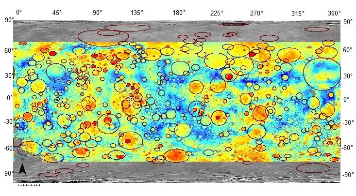

Fig 1: DTM of Mercury’s topography. Circles mark the identified basins.
Results
Our preliminary basin inventory hosts 311 basins (Fig.1). A clear correlation is noticed between the topography and gravity data, in particular impact basins are well detectable in both data sets. Their global distribution is non-uniform. Around 60% of basins are located on the western hemisphere. This asymmetric pattern may be caused by (I) lateral thermal variances of the crust [1], (II) synchronous spin- and orbital periods of the planet in its early history, which later changed to its presently observed 3:2 spin-orbit resonance [2], (III) resurfacing events that includes the northern smooth plains and following flooding of existing basins on the eastern hemisphere, which would eventually bury smaller complex basins.
With increasing diameter basins were found to show more complex gravity- and topography signatures. Basins with smaller diameter (<160 km) display a central peak. With increasing size, the morphology changes to a peak ring in the center. The transition from peak ring to multi-ring basins is suggested to occur at 350 km as is attested by a distinct change in the gravitational signal. The gravity disturbance remains mostly in strong negative values. This value shifts to a positive one for basins larger than 350 km.
High positive gravity signals were also recognized in the Bouguer anomaly map. Some basins (>350 km) possess a positive Bouguer anomaly in the basin center surrounded by a negative anomaly annulus (bullseye pattern) (Fig 2). Gravity data are reflecting mass/density deficits and excesses in the planet’s subsurface structures. The high mass and density concentrations may be caused by an uplift of mantle material after the crater excavation phase [5]. The excavation was followed by an isostatic adjustment caused by cooling and contraction of the melt pool. Subsequently, crust is expected to be thinner.

Fig 2: Left: Profile of Bouguer anomaly, Right: Bouguer anomaly map; showing positive strong anomaly in center surrounded by negative annulus.
However, basins with small diameter (<200 km) were found to show strong positive anomalies as well, that indicate a mantle uplift after their formations. Due to limited data resolution (particularly in the south) the localization and accuracy of the Bouguer anomalies is not certain.
Other 208 basins where identified, but could not be characterized in detail due to their high degradation state (rim <50%). Most of these are filled by secondary material. Future data with improved resolution would be required to verify these results.
We investigated the amplitude of Bouguer anomalies in the basin centers and surroundings as a measure of crustal thinning, which may hint at basin relaxation state. Lunar observations showed, that young basins with large diameters should contain strong positive anomalies because of limited relaxation due to high viscosity of a cooler planet [6]. In contrast, a less pronounced gravity anomalies hint at higher relaxation due to lower viscosity and a hotter crust in the planet’s earlier history (Fig 3).

Fig. 3: Bouguer anomaly contrast from rim to centre versus rim diameter. Basin classes: b_deg- degraded basin (<50% rim preserved), centr_peak- central peak basin, peakr- peak ring basin, com- complex basin (>50% rim preserved).
Acknowledgements
This work is supported by the Deutsche Forschungsgemeinschaft (SFB-TRR170, A6).
References
[1] Orgel et al., 2020, Re-examination of the Population, Statigraphy and Sequence of Mercurian Basins: Implications for Mercury’s Early Impact History and Comparison with the Moon, J. Geophys. Res. 125(8), doi:10.1029/2019JE006212
[2] Fassett C. I., et al., (2012), Large impact basins on Mercury: Global distribution, characteristics, and modification history from MESSENGER orbital data, J. Geophys. Res. 117, E00L08, doi:10.1029/2012JE004154
[3] Preusker et al., Towards high-resolution global topography of Mercury from MESSENGER orbital stereo imaging: A prototype model for the H6 (Kuiper) quadrangle, Planetary and Space Science 142 (2017) 26-37
[4] Konopliv et al., The Mercury gravity field, orientation, love number, and ephemeris from the MESSENGER radiometric tracking data, Icarus, Volume 335, 2020, 113386, ISSN 0019-1035,https://doi.org/10.1016/j.icarus.2019.07.020.
[5] Wieczorek, M., The gravity and topography of terrestrial planets, Treatise on geophysica, 2006
[6] Neumann et al., 2015. Lunar impact basins revealed by Gravity Recovery and Interior Laboratory measurements. Science Advances 1(9), 1-10.
How to cite: Szczech, C. C., Oberst, J., and Preusker, F.: Classification of Mercury’s Impact Basins, Based on Topography- and Gravity Signatures in MESSENGER Data, Europlanet Science Congress 2022, Granada, Spain, 18–23 Sep 2022, EPSC2022-595, https://doi.org/10.5194/epsc2022-595, 2022.
Data from NASA MESSENGER spacecraft highlighted that Mercury’s surface and composition are more varied than previously thought. Despite being the closest planet to the Sun, indeed, Mercury is rich in volatiles and its surface shows evidence of volatile-driven processes such as the formation of hollows and explosive volcanism. Even MESSENGER’s color-derived basemaps, moreover, highlight relevant color variations of the hermean surface possibly indicating age and compositional differences between adjacent materials.
The ongoing mapping for the eastern H9 Eminescu quadrangle (22.5°N-22.5°S, 108°E-144°E) [1] led to a thorough knowledge of the area that allowed the definition of scientific targets of interest to be investigated by the SIMBIO-SYS cameras [2] onboard the ESA-JAXA BepiColombo mission [3] coupled with other instruments such as MERTIS, BELA, MGNS and MIXS.
Proposed targets range from hollows to volcanic features, from craters and deformational structures and specific terrains and aim at shedding light on scientific questions concerning Mercury’s origin and evolution [4]. In particular, proposed targets aim to i) determine the abundance and distribution of key elements, minerals and rocks on the hermean crust, ii) characterize and correlate geomorphological features with compositional variations, iii) investigate the nature, evolution, composition and mechanisms of effusive and explosive events, iv) determine the formation and growth rates of hollows, the nature of processes related with volatile loss and their mineralogical and elemental composition of volatiles, v) determine the displacement and kinematics of tectonic deformations and the mechanisms responsible for their formation and vi) verify the occurrence of any detectable change in and around hollows and pyroclastic deposits since MESSENGER observations.
Acknowledgements: We acknowledge support from the Italian Space Agency (ASI) under ASI-INAF agreement 2017-47-H.0.
References: [1] El Yazidi et al., 2021, EPSC. [2] Cremonese et al., 2020, Sp. Sci. Rev. [3] Benkhoff et al., 2010, Plan. Sp. Sci. [4] Rothery et al., 2020, Sp. Sci. Rev.
How to cite: Tognon, G. and Massironi, M.: Definition of scientific targets of interest for BepiColombo in the eastern Eminescu (H9) quadrangle, Europlanet Science Congress 2022, Granada, Spain, 18–23 Sep 2022, EPSC2022-624, https://doi.org/10.5194/epsc2022-624, 2022.
Introduction: The IRIS (Infrared and Raman for Interplanetary Spectroscopy) laboratory generates mid-infrared spectra for the ESA/JAXA BepiColombo mission to Mercury. Onboard is a mid-infrared spectrometer (MERTIS-Mercury Radiometer and Thermal Infrared Spectrometer), which will allow to map the mineralogy in the 7-14 µm range [1, 2]. In order to interpret the future data, a database of laboratory spectra is assembled at the Institut für Planetologie in Münster (IRIS) and the DLR in Berlin.
So far, we have studied for this purpose natural mineral and rock samples (e.g. 3, 4), impact melt rocks (e.g. 5, 6, 7) and meteorites (e.g. 8, 9, 10, 11). Furthermore, surface processes like regolith formations and space weathering were of interest (e.g. 12, 13, 14).
Synthetic analogue materials have become one of the foci of our work, since they allow to produce ‘tailor-made’ materials based on remote sensing data and/or modelling and experiments. These are closer than natural terrestrial materials, which formed usually under different conditions as expected on Mercury [e.g. 1]. We synthesized analogs for surface regions of Mercury and other planetary bodies (15, 16, 17).
In this part of our study, we present mixtures based on phase equilibria of peridotite and partial melt compositions which were studied under hermean mantle conditions - temperature, pressure, oxygen fugacity (18,19,20). These experiments suggested that the crustal mineralogy should be dominated by variable abundances of plagioclase, olivine, clino- and orthopyroxene, with unconstrained proportions of silicate glass. Based on the model mineralogy of representative results, we produced mineral/glass mixtures based on the Low-Mg Northern Volcanic Plains (NVP)(Y121, Y131, Y172), High-Mg NVP (Y143, Y144), Smooth Plains (Y140, Y143, Y144), Inter crater Plain and Heavily Cratered Terrains (IcP-HCT) (Y126, Y131, Y132, Y146), and High-Mg Province (Y126, Y131, Y146) [20].
Samples and Techniques: We conducted diffuse reflectance studies of sieved size fractions (0-25 µm, 25-63 µm, 63-125 µm and 125-250 µm) under vacuum conditions, ambient heat, and variable geometries. We used a Bruker Vertex 70v with A513 variable geometry stage. The results will be made available in the IRIS Database [1].
Results: First results show the Christiansen Feature (CF), a characteristic, easy to identify reflectance low (or emission high) ranging from 7.9 µm to 8.2 µm (always average of all size fractions). The Transparency Feature (TF), typical for the finest size fraction (0-25 µm) is in many mineral mixtures less pronounced than for pure mineral phases. Here the individual TF of the components result in a broad feature.
The resulting spectra can be divided into three groups – such as dominated by a single glass feature at 9.6 – 9.9 µm, a second groups with forsterite bands 9.4 µm- 9.5 µm, 10.2 µm, 10.6 µm, 11.9 µm and 15.9 µm-16 µm, and a third dominated by pyroxene bands at 8.9-9.1 µm, 9.4-9.5 µm, 9.9 µm, 10.2 µm, 10.4-10.5 µm, 10.6 µm, 10.8-11 µm 11.1-11.3 µm and 11.4-11.6 µm. Plagioclase features, even when the phase is dominating the composition, are usually ‘overprinted’ by forsterite and pyroxene bands.
Discussion: A classic way to connect an easy to identify spectral feature in the mid-infrared to the chemical bulk composition is using the CF and the SiO2 content. Both show a strong correlation for both terrestrial rocks [21] and a variety of synthetic analogue samples from earlier studies in this project [15, 16, 17] (Fig.1).
Summary & Conclusion: In a next step, we will study these mixtures under more realistic conditions, i.e., high vacuum and high temperature, in order to better simulate the hermean surface. Also, these mixtures will be used to test spectral unmixing routines, which allow to identify abundances of single minerals in a complex mixture of phases.
References: [1] Hiesinger et al. (2020) Space Sci. rev. 216, 110 [2] Benkhoff et al. (2022) Space Sci. Rev. 217, 90 [3] Reitze et al.(2020) Min. Pet. 114, 453-463 [4] Reitze et al.(2021) EPSL 554, 116697 [5] Morlok et al.(2016) Icarus 264, 352-368 [6] Morlok et al.(2016) Icarus 278, 162-179 [7] Reitze et al.(2021) JGR (Planets) 126, e06832 [8] Weber et al. (2016) MAPS 51, 3-30 [9] Morlok et al. (2017) Icarus 284, 431-442 [10] Morlok et al. (2020) MAPS 55, 2080-2096 [11] Martin et al. (2017) MAPS 52, 1103-1124 [12] Weber et al. (2020) EPSL 530, 115884 [13] Weber et al. (2021) EPSL 569, 117072 [14] Stojic et al. (2021) Icarus 357, 114162 [15] Morlok et al. (2017) Icarus 296, 123-138 [16] Morlok et al. (2019) Icarus 324, 86-103 [17] Morlok et al. (2021) Icarus 361, 114363 [18] Charlier et al. (2013) EPSL 363, 50-60 [19] Namur et al. (2016) EPSL 439, 117-128 [20] Namur and Charlier (2017) Nature Geosci. 10, 9-13 [21] Cooper at al. (2002) JGR 107, 5017-5034 [22] Morlok et al. (2020) Icarus 335, 113410
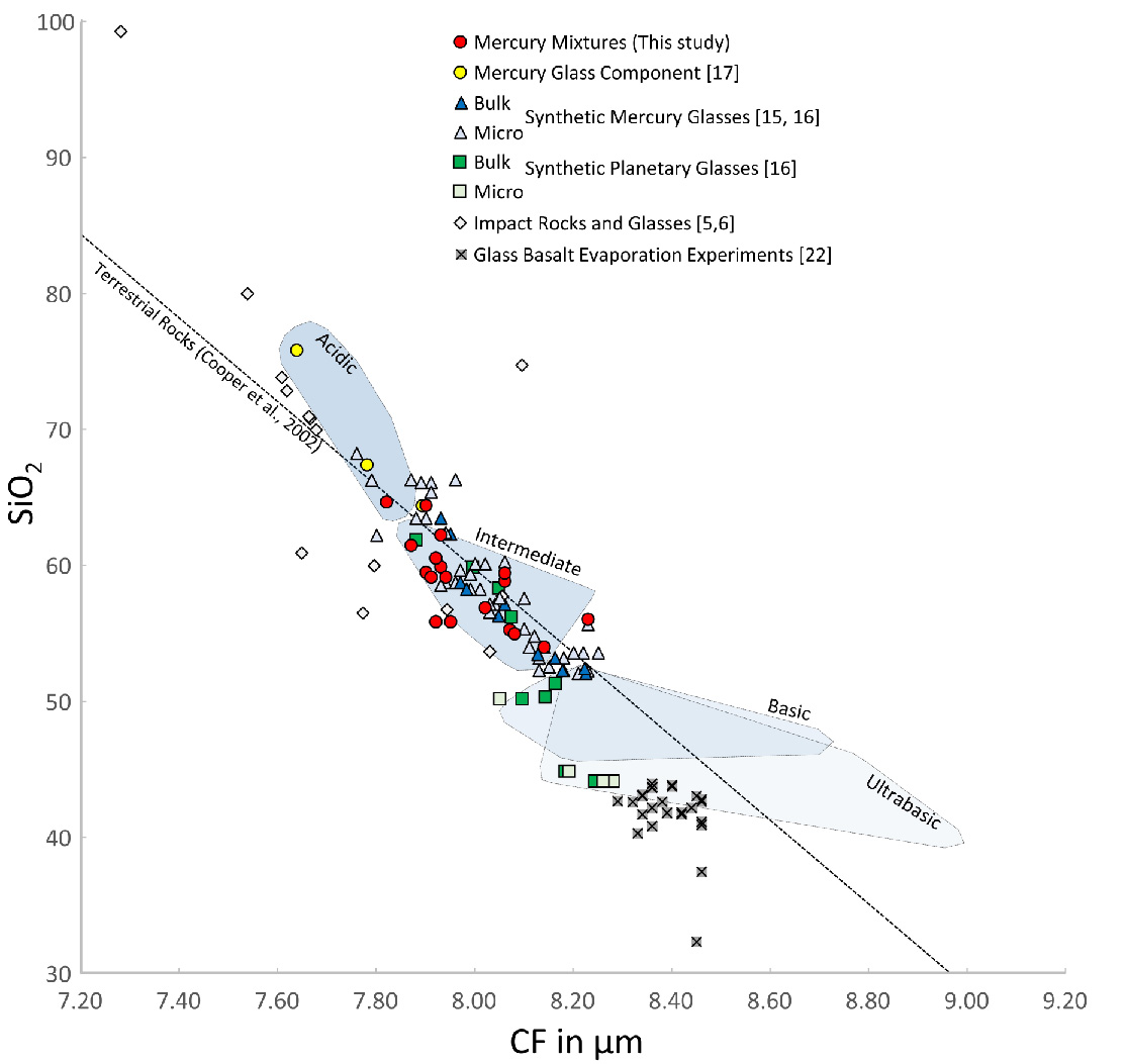
Figure 1: Comparison of the Christiansen Feature (CF), a characteristic reflectance low, to the SiO2 bulk composition. The results from this study (red circles) fall along the regression line for terrestrial intermediate rocks.
How to cite: Morlok, A., Renggli, C., Charlier, B., Namur, O., Klemme, S., Reitze, M., Weber, I., Stojic, A. N., Bauch, K., Schmedemann, N., Pasckert, J.-H., Hiesinger, H., and Helbert, J.: Synthetic Analogs for Surface Regions on Mercury: A Mid-Infrared Study for the BepiColombo Mission, Europlanet Science Congress 2022, Granada, Spain, 18–23 Sep 2022, EPSC2022-876, https://doi.org/10.5194/epsc2022-876, 2022.
The low intensity and lack of small-scale variations in Mercury’s present-day magnetic field can be explained by a thermally stratified layer blanketing the convective liquid outer core. The presence of a present-day stable layer is supported by thermal evolution studies that show that a sub-adiabatic heat flow at the core-mantle boundary can occur during a significant fraction of Mercury’s history. The requirements for both the likely long-lived Mercury dynamo and the presence of a stable layer place important constraints on the interior structure and evolution of the core and planet.
We couple mantle and core thermal evolution to investigate the necessary conditions for a long-lived and present-day dynamo inside Mercury’s core by taking into account an evolving stable layer overlying the convecting outer core. Events such as the cessation of convection in the mantle may strongly influence the core-mantle boundary heat flow and affect the thickness of the thermally stratified layer in the core, highlight the importance of coupling mantle evolution with that of the core. We employ interior structure models that agree with geodesy observations and make use of recent equations of state to describe the thermodynamic properties of Mercury’s Fe-S-Si core for our thermal evolution calculations.
How to cite: Rivoldini, A., Deprost, M.-H., Zhao, Y., Knibbe, J., and Van Hoolst, T.: Effect of a thermally stratified layer in the outer core of Mercury on its internally generated magnetic field, Europlanet Science Congress 2022, Granada, Spain, 18–23 Sep 2022, EPSC2022-929, https://doi.org/10.5194/epsc2022-929, 2022.
Since the era of Messenger, many observational constraints on Mercury’s thermal evolution and magnetic field have strengthened the idea that the outermost layer of Mercury’s fluid core is stably stratified. The presence of such a stably stratified zone can significantly alter the core flow compared to the flow in a completely homogeneous fluid core. This is on the one hand because stratified layers can impede fluid motions that are parallel to the density gradient, which in the case of Mercury would mean that radial flows are strongly suppressed. On the other hand this is because a stably stratified layer can support different types of waves that are affected by the buoyancy force.
In this study we have created a numerical model to investigate flow in Mercury’s fluid outer core that includes a radial background stratification. The exact structure of the density profile in the planet’s core is unknown, and we assume profiles based on recent findings of the interior evolution of the planet. We studied core flow that is excited by Mercury’s librations, oscillations of the mean rotation rate due to the solar gravitational torque acting on Mercury’s triaxial shape. Based on the work by Rekier et. al. (2019) we represent the librational forcing by the superposition of three different decoupled motions: a horizontal component, which represents the viscous drag of the core fluid by the librating mantle and spherical inner core, and two radial components that are representing the radial push that the core flow would experience due to the librating triaxial boundaries.
We show that especially the second component has a profound effect, inducing a large non-axisymmetric flow close to the core-mantle boundary. It turns out that even though the origin of said flow is radial, the horizontal component of the flow is far larger than it’s radial counterpart. This indicates that the stratified layer acts to convert radial motions into strong horizontal motions.
We show how the strength and existence of this flow depend on the strength of the stratification of the layer and discuss implications of this flow for the magnetic field.
References:
Rekier, J., Trinh, A., Triana, S. A., & Dehant, V. (2019). Internal energy dissipation in Enceladus's subsurface ocean from tides and libration and the role of inertial waves. Journal of Geophysical Research: Planets, 124, 2198–2212. https://doi.org/10.1029/2019JE005988
How to cite: Seuren, F., Rekier, J., Triana, S. A., and Van Hoolst, T.: The core flow induced by Mercury’s libration: density stratification and magnetic fields, Europlanet Science Congress 2022, Granada, Spain, 18–23 Sep 2022, EPSC2022-934, https://doi.org/10.5194/epsc2022-934, 2022.
TP2 | Paving the way to the decade of Venus
Background
In situ probe measurements and remote sensing have revealed that Venus has a highly organised cloud system. Comparisons between models of the expected spectra and observations reveal unexplained absorption in the near-UV to blue region of the spectrum. While many candidates for this “unknown absorber” have been proposed over the years, none have been conclusively demonstrated to match the physical and optical behaviour observed (Pérez-Hoyos et al., 2018, JGR Planets, 123).
One such candidate is ferric chloride (Krasnopolsky, 2017, Icarus, 286; Zasova et al., 1981, ASR, 1). Attempts to reliably determine its suitability have been hampered by the scarcity of representative spectra available. Absorbance spectra generally used in the literature are measured in ethyl acetate (Aoshima et al., 2013, Polymer Chemistry, 4), and therefore may not be representative of the absorption produced by ferric chloride in the Venusian clouds.
In addition to the absorption spectrum produced, the behaviour of absorber candidates must also be considered, including their rates and locations of production and loss, transport mechanisms, and lifetimes in the atmosphere. While much of this behaviour must be examined in atmospheric models, laboratory studies to establish reaction pathways and measure rates are needed to provide as much quantitative data as possible for model development.
Method and results
Literature spectra for ferric chloride employ UV-visible spectrometry using ethyl acetate as a solvent. We present absorption spectra of ferric chloride in sulphuric acid. This change of solvent produces an environment more closely aligned to that on Venus, where ferric chloride, if present, may exist as an impurity in the micron-sized sulphuric acid cloud droplets (Petrova, 2018, Icarus, 306).
In addition, mass spectrometry was used to investigate the kinetics and products of reactions of ferric chloride that could occur in the Venusian atmosphere. Behaviour predicted by these experiments can then be included in atmospheric models to test the lifetime and transport of ferric chloride and its reaction products in the atmosphere.
Conclusions
The unknown absorption was first observed close to 100 years ago, yet the mystery of its cause remains unsolved. More representative spectra of ferric chloride and a greater understanding of its behaviour in the atmosphere of Venus are critical to advancing the identification of the unknown absorber. As the absorber is located towards the top of the clouds and absorbs in the near-UV to blue region, it is responsible for large amounts of absorption of incident sunlight, and therefore has a significant impact on the Venusian energy budget. Accurate atmospheric modelling of the planet therefore requires an understanding of the absorber which can only be achieved once it has been conclusively identified.
How to cite: Egan, J., James, A., Plane, J., Murray, B., and Feng, W.: Laboratory experiments to constrain the identity of Venus’s unknown UV absorber, Europlanet Science Congress 2022, Granada, Spain, 18–23 Sep 2022, EPSC2022-76, https://doi.org/10.5194/epsc2022-76, 2022.
Observations of the Venus Climate Orbiter “Akatsuki” provide us with horizontal distributions of the horizontal winds derived from cloud tracking of the Ultraviolet Imager (UVI) and of temperature observed by the Longwave Infrared Camera (LIR). However, these observations are limited in altitude, local time (day or night side), and frequency. Then it is difficult to elucidate the general circulation of the Venus atmosphere, including various temporal and spatial scales, only from observations. In this study, we produced a Venus dataset (analysis) that has high temporal and spatial resolutions by assimilating horizontal winds derived by the Akatsuki observations. At the top of the cloud layer of Venus, there are planetary-scale atmospheric waves that are excited by the solar heating and move with the sun, called the thermal tides. In this presentation, we focused on thermal tides to verify the analysis.
We use the Venus atmospheric data assimilation system “ALEDAS-V" (Sugimoto et al., 2017) [1] for assimilation and the Venus atmospheric general circulation model “AFES-Venus" (Sugimoto et al., 2014) [2] for ensemble forecasts. AFES-Venus is a full nonlinear dynamical GCM on the assumption of hydrostatic balance, designed for the Venus atmosphere. ALEDAS-V uses the Local Ensemble Transform Kalman Filter, and is the first data assimilation system for the Venus atmosphere. We assimilated the cloud top (~70km) zonal and meridional winds obtained by tracking morphology, using Akatsuki UVI data (Horinouchi et al., 2021) [3] from September 1st to December 31st, 2018. The assimilation data (analysis) from October 1st to November 30th, 2018, is analyzed, because the root-mean-square-deviations (RMSD) from FR (free run; the case without data assimilation) are stable.
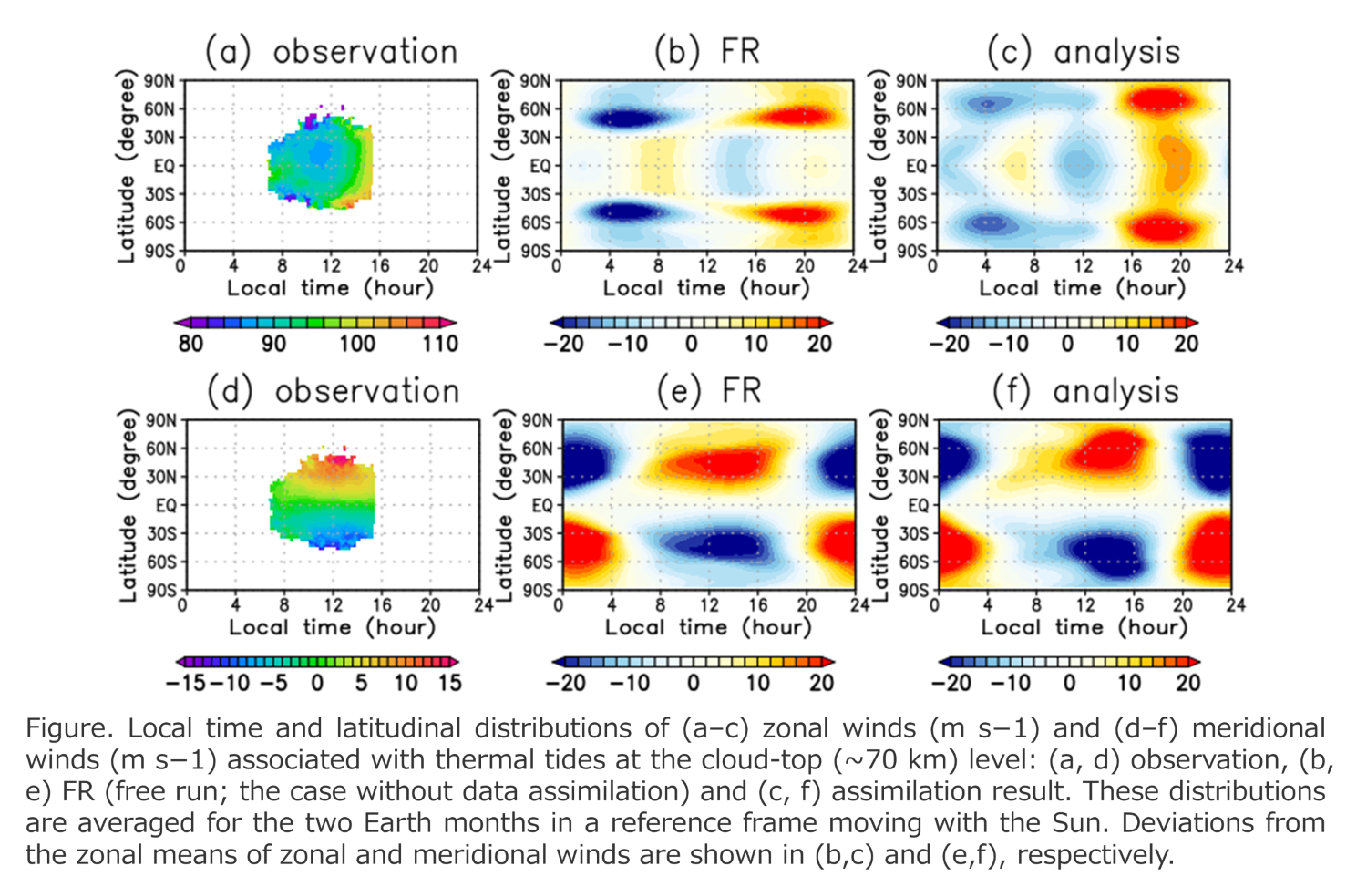
Figures (a) and (d) show the observed zonal and meridional winds, respectively. The zonal wind has a local minimum near 11 LT (local time) around the equator (Figure a). The meridional wind is the weakest at the equator and increases with latitude, and the amplitude is maximum around noon (Figure d) in the local time direction. Note that these winds obtained from observations exist only the dayside equatorward of 50° latitudes (Figure a and d).
Figures (b) and (e) show the deviations from the zonal means of zonal and meridional winds at an altitude of 70 km in the FR, respectively. For zonal wind, diurnal (zonal wavenumber 1) and semidiurnal (zonal wavenumber 2) tides are dominant at latitudes poleward and equatorward of 30, respectively (Figure b). The zonal wind deviation has a local minimum at 14-15LT, which is ~ 2 hours behind the observation (Figures a and b). The meridional wind deviation is polar and equatorial on the dayside and nightside, respectively (Figure e), and this distribution is consistent with Akatsuki's observation (Figure d).
Figures (c) and (f) show the zonal and meridional winds as a result of assimilation, respectively. The zonal wind in the equatorial region have a local minimum near 11 LT. The assimilation improved the semidiurnal tide closer to the observations (Figures a and c). The meridional wind is not so different from FR. This is probably because FR was originally very similar to observations (Figures d and f). These results are consistent with a previous study by Sugimoto et al. (2019) [4]. In addition, while the observed winds exist only on the dayside, the results of assimilation show that the horizontal winds field is modified significantly even on the nightside. It is suggested that spatially limited data assimilation can improve the general circulation of GCM.
In the future work, we are planning to release the assimilation dataset as the “objective analysis data” of Venus for the first time in the world.
[1] Sugimoto, N., et al. Development of an ensemble Kalman filter data assimilation system for the Venusian atmosphere. Scientific Reports 7(1), 9321 (2017).
[2] Sugimoto, N., et al. Baroclinic instability in the Venus atmosphere simulated by GCM. J. Geophys. Res. Planets 119, 1950–1968 (2014).
[3] Horinouchi, T., et al. Venus Climate Orbiter Akatsuki Cloud Motion Vector Data Set v1.0, JAXA Data Archives and Transmission System (2021).
[4] Sugimoto, N., et al. Impact of data assimilation on thermal tides in the case of Venus Express wind observation. Geophys. Res. Lett. 46, 4573–4580 (2019).
How to cite: Fujisawa, Y., Murakami, S., Sugimoto, N., Takagi, M., Imamura, T., Horinouchi, T., Hashimoto, G. L., Ishiwatari, M., Enomoto, T., Miyoshi, T., Kashimura, H., and Hayashi, Y.-Y.: Thermal tides reproduced in the assimilation results of horizontal winds obtained from Akatsuki UVI observations, Europlanet Science Congress 2022, Granada, Spain, 18–23 Sep 2022, EPSC2022-309, https://doi.org/10.5194/epsc2022-309, 2022.
Since 2012, we have been monitoring SO2 and H2O (using HDO as a proxy) at the cloud top of Venus, using the TEXES high-resolution imaging spectrometer at the NASA InfraRed Telescope Facility (IRTF) at Maunakea Observatory. Sixteen runs have been performed between 2012 and 2022. Maps have been recorded around 1345 cm-1 (7.4 microns, z = 62 km), where SO2, CO2 and HDO are observed, and around 530 cm-1 (19 microns, z = 57 km) where SO2 and CO2 are observed, as well as around 1162 cm-1 (8.6 microns, z = 66 km) where CO2 is observed. From the early beginning, SO2 plumes have been identified with an evolution time scale of a few hours. In 2020, an anti-correlation has been found in the long-term evolution of H2O and SO2; in addition, the SO2 plume appearance as a function of local time seems to show two maxima around the terminator, indicating the possible presence of a semi-diurnal wave (Encrenaz et al. A&A 639, A69, 2020). After two years of interruption due to the pandemia, new observations have been performed in July 2021, September 2021, November 2021, and February 2022. The main results of the new observations are listed below. (1)The SO2 abundance, which had been globally increasing from 2014 until 2019, has now decreased with respect to its maximum value. (2) The anti-correlation between H2O and SO2, which was maximum between 2014 and 2019 (cc = - 0.9) does not appear clearly in the recent observations. (3) The maximum appearance of the SO2 plumes at the equator and the terminators is confirmed, but appears stronger on the morning side.(4) A strong activity of the SO2 plumes is observed in September and November 2021, at a time when the disk-integrated SO2 abundance is low. At the same time, thermal maps at 1162 cm-1 (8.6 microns, z = 66 km) show a polar enhancement. This behavior could possibly be associated with the topography.
How to cite: Encrenaz, T., Greathouse, T., Giles, R., Widemann, T., Bézard, B., and Fouchet, T.: Ground-based HDO and SO2 thermal mapping on Venus between 2012 and 2022: : An update, Europlanet Science Congress 2022, Granada, Spain, 18–23 Sep 2022, EPSC2022-414, https://doi.org/10.5194/epsc2022-414, 2022.
Numerical simulation of Venus’ atmosphere is useful to understand the dynamics of the system. The Venus atmospheric data assimilation system “ALEDAS-V” (Sugimoto et al. 2017) based on the Venus atmospheric general circulation model “AFES-Venus” (Sugimoto et al. 2014) has been used to simulate Venus’ atmosphere and generated some key phenomena such as the super-rotation, baroclinic waves, and thermal tides. To further understand the dynamics of Venus’ atmosphere, Bred Vectors (BV) are computed with the AFES-Venus model. This method can identify different growing modes of the system and has been used to study the dynamics of the Earth (Toth and Kalnay 1993, 1997) and Martian atmospheres (Greybush et al. 2013). However, to our knowledge, there has been no similar study on Venus’ atmosphere. To conduct the breeding cycle, we first produced a five (Earth) year free run of the AFES-Venus model initialized from an idealized zonal wind profile. Next, the forecast states on January 01 and August 25 in the 5th Earth year are used as the initial conditions for the control run and the perturbed run, respectively. These two initial conditions have the same sub-solar positions. To emphasize the active dynamics, the BV norm is defined by the temperature norm from the 60 km to 80 km altitudes, weighted by pressure and latitude. For the breeding cycle, a rescaling norm and rescaling interval are specified. During the breeding cycle, at every rescaling interval (including the initial time), if the norm is bigger than the specified rescaling norm, the BV is rescaled to the rescaling norm.
Different combinations of the parameters are tested. The BV amplitude generally remains stable throughout the whole year without significant seasonal variability (Figure 1), which is different from the Martian atmosphere. The growth rate of the BV amplitude can represent the characteristics of the instabilities. It is calculated by taking the natural logarithm of the ratio of the BV amplitude at the end of the time interval (before rescaling) to the amplitude at the beginning of the interval. It is then converted to the daily growth rate by dividing the ratio of the time interval to one day. When the rescaling norm is smaller or the rescaling interval is shorter, the average growth rate is higher (Figure 2). Further BV analysis will be conducted such as analyzing the BV structure by taking composite mean along the super-rotation and conducting BV breeding cycle without thermal tides. These results will be useful to understand the dynamics of the thermal tide, baroclinic waves, super-rotation, and other important features of Venus atmosphere.

Figure 1. The bred vector amplitude (K2 ) time evolution from the experiments with different rescaling days (1, 2, 5, 10, 20) and the same rescaling norm (10 K2 ).

Figure 2. The average daily growth rate of the bred vector amplitude (K2 ) for different combination of rescaling norm and rescaling days. The average is taken from February to December.
Reference
Greybush, S. J., E. Kalnay, M. J. Hoffman, and R. J. Wilson, 2013: Identifying Martian atmospheric instabilities and their physical origins using bred vectors. Q. J. R. Meteorol. Soc., 139, 639–653, https://doi.org/10.1002/qj.1990.
Sugimoto, N., M. Takagi, and Y. Matsuda, 2014: Baroclinic instability in the Venus atmosphere simulated by GCM. J. Geophys. Res. Planets, 119, 1950–1968, https://doi.org/10.1002/2014JE004624.
——, A. Yamazaki, T. Kouyama, H. Kashimura, T. Enomoto, and M. Takagi, 2017: Development of an ensemble Kalman filter data assimilation system for the Venusian atmosphere. Sci. Rep., 7, 9321, https://doi.org/10.1038/s41598-017-09461-1.
Toth, Z., and E. Kalnay, 1993: Ensemble Forecasting at NMC: The Generation of Perturbations. Bull. Am. Meteorol. Soc., 74, 2317–2330, https://doi.org/10.1175/1520-0477(1993)074<2317:EFANTG>2.0.CO;2.
——, and ——, 1997: Ensemble Forecasting at NCEP and the Breeding Method. Mon. Weather Rev., 125, 3297–3319, https://doi.org/10.1175/1520-0493(1997)125<3297:EFANAT>2.0.CO;2.
How to cite: Liang, J., Sugimoto, N., and Miyoshi, T.: Identifying the growing modes of Venus’ atmosphere using Bred Vectors, Europlanet Science Congress 2022, Granada, Spain, 18–23 Sep 2022, EPSC2022-713, https://doi.org/10.5194/epsc2022-713, 2022.
We report on detection and upper-limit of H2CO, O3, NH3, HCN, N2O, NO2, and HO2 above the cloud deck using the SOIR instrument on-board Venus Express.
The SOIR instrument performs solar occultation measurements in the IR region (2.2 - 4.3 µm) at a resolution of 0.12 cm-1, the highest of all instruments on board Venus Express. It combines an echelle spectrometer and an AOTF (Acousto-Optical Tunable Filter) for the order selection. SOIR performed more than 1500 solar occultation measurements leading to about two millions spectra.
The wavelength range probed by SOIR allows a detailed chemical inventory of the Venus atmosphere at the terminator in the mesosphere, with an emphasis on vertical distribution of the gases.
In this work, we report detections in the mesosphere, between 60 and 100 km.
Implications for the mesospheric chemistry will also be addressed.
How to cite: Mahieux, A., Robert, S., Mills, F., Trompet, L., Aoki, S., Piccialli, A., Jessup, K. L., and Vandaele, A. C.: Minor species in the Venus mesosphere from SOIR on board Venus Express: detection and upper limit profiles of H2CO, O3, NH3, HCN, N2O, NO2, and HO2, Europlanet Science Congress 2022, Granada, Spain, 18–23 Sep 2022, EPSC2022-921, https://doi.org/10.5194/epsc2022-921, 2022.
Venus appears to be an “alien” planet drastically and surprisingly different from the Earth. The early space missions revealed the world with remarkably hot, dense, cloudy, and very dynamic atmosphere filled with toxic species likely of volcanic origin. During more than 8 years of operations ESA’s Venus Express spacecraft performed a global survey of the atmosphere and plasma environment of our near neighbour. The mission delivered comprehensive data on the temperature structure, the atmospheric composition, the cloud morphology, the atmospheric dynamics, the solar wind interaction and the escape processes. Vertical profiles of the atmospheric temperature showed strong latitudinal trend in the mesosphere and upper troposphere correlated with the changes in the cloud top structure and suggesting convective instability in the main cloud deck at 50-60 km. Observations revealed significant latitudinal variations and temporal changes in the global cloud top morphology, which modulate the solar energy deposited in the atmosphere. The cloud top altitude varies from ~72 km in the low and middle latitudes to ~64 km in the polar region, correlated with decrease of the aerosol scale height from 4 ± 1.6 km to 1.7 ± 2.4 km, marking vast polar depression. UV imaging showed for the first time the middle latitudes and polar regions in unprecedented detail. In particular, the eye of the Southern polar vortex was found to be a strongly variable feature with complex dynamics.
Solar occultation observations and deep atmosphere spectroscopy in spectral transparency “windows” mapped distribution of the major trace gases H2O, SO2, CO, COS and their variations above and below the clouds, revealing key features of the dynamical and chemical processes at work. A strong, an order of magnitude, increase in SO2 cloud top abundance with subsequent return to the previous concentration was monitored by Venus Express specrometres. This phenomenon can be explained either by a mighty volcanic eruption or atmospheric dynamics.
Tracking of cloud features provided the most complete characterization of the mean atmospheric circulation as well as its variability. Low and middle latitudes show an almost constant with latitude zonal wind speed at the cloud tops and vertical wind shear of 2-3 m/s/km. Surprisingly the zonal wind speed was found to correlate with topography decreasing from 110±16 m/s above lowlands to 84±20 m/s at Aphrodite Terra suggesting decelerating effect of topographic highs. Towards the pole, the wind speed drops quickly and the apparent vertical shear vanishes. The meridional cloud top wind has poleward direction with the wind speed ranging from about 0 m/s at equator to about 15 m/s in the middle latitudes. A reverse equatorward flow was found about 20 km deeper in the middle cloud suggesting existence of a Hadley cell or action of thermal tides at the cloud level. Comparison of the thermal wind field derived from temperature sounding to the cloud-tracked winds confirms the validity of cyclostrophic balance, at least in the latitude range from 30S to 70S. The observations are supported by the General Circulation Models.
Venus Express detected and mapped non-LTE infrared emissions in the lines of O2, NO, CO2, OH originating near the mesopause at 95-105 km. The data show that the peak intensity occurs in average close to the anti-solar point for O2 emission, which is consistent with current models of the thermospheric circulation. For almost complete solar cycle the Venus Express instruments continuously monitored the induced magnetic field and plasma environment and established the global escape rates of 3·1024s−1, 7·1024s−1, 8·1022s−1 for O+, H+, and He+ ions and identified the main acceleration process. For the first time it was shown that the reconnection process takes place in the tail of a non-magnetized body. It was confirmed that the lightning tentatively detected by Pioneer-Venus Orbiter indeed occurs on Venus.
Thermal mapping of the surface in the near-IR spectral “windows” on the night side indicated the presence of recent volcanism on the planet, as does the high and strongly variable SO2 abundance. Variations in the thermal emissivity of the surface observed by the VIRTIS imaging spectrometer indicated compositional differences in lava flows at three hotspots. These anomalies were interpreted as a lack of surface weathering suggesting the flows to be younger than 2.5 million years indicating that Venus is actively resurfacing. The VMC camera provided evidence of transient bright spots on the surface that are consistent with the extrusion of lava flows that locally cause significantly elevated surface temperatures. The very strong spatial correlation of the transient bright spots with the extremely young Ganiki Chasma, their similarity to locations of rift-associated volcanism on Earth, provide strong evidence of their volcanic origin and suggests that Venus is currently geodynamically active.
Alongside observations of Earth, Mars and Titan, observation of Venus allows the opportunity to study geophysical processes in a wide range of parameter space. Furthermore, Venus can be considered as an archetype of terrestrial exoplanets that emphasizes an important link to the quickly growing field of exoplanets research.
The talk will give an overview of the Venus Express findings including recent results of data analysis, outline outstanding unsolved problems and provide a bridge, via the Akatsuki mission, to the missions to come in 2030s: EnVision, VERITAS and DAVINCI.
How to cite: Titov, D., Straume-Lindner, A. G., and Wilson, C.: Venus Express as precursor of the Venus Decade, Europlanet Science Congress 2022, Granada, Spain, 18–23 Sep 2022, EPSC2022-1120, https://doi.org/10.5194/epsc2022-1120, 2022.
TP3 | Forward to the Moon: The Science of Exploration
1. Introduction
Knowing the photometric properties of a surface can give us insight into its physical properties. Images with several different observation conditions can be used to constrain the parameters of a semi-physical model like the Hapke model [1].
The Wide Angle Camera onboard the Lunar Reconnaissance Orbiter (LROC WAC) [2] provides unprecedented coverage of the lunar surface for a variety of phase angles. The field of view of the Narrow Angle Camera (LROC NAC) [2] is much smaller and therefore, also the possible phase angles are limited but the resolution is around 1 m/pixel.
Sato et al. [3] have used WAC images to create global maps of the Hapke parameters binned into areas of 1 degree/pixel [3]. In this work, we calculate photometric parameters on the pixel level. Velikodsky et al. [4] investigated the relative contributions of coherent backscatter and shadow hiding opposition effects based on WAC images and, similar to [3], find that the total strength of the opposition effect is inversely correlated with albedo.
The landing of a spacecraft on the lunar surface can change the physical properties of the regolith [5], e.g., by compacting the very porous lunar regolith.
2. Methods
Our method consists of three main steps. Firstly, the WAC or NAC EDR images are downloaded from the PDS and processed with ISIS3 [6]. This process includes calibration and map projection. The NAC images are mapped to a common resolution of 1.6 m/pixel and the WAC images are mapped to a resolution of 400 m/pixel. The sub-solar and sub-spacecraft points are extracted using the campt command in ISIS3.
Secondly, suitable images are co-registered in MATLAB to a common reference image and we calculate the incidence, emission, and phase angles based on the trajectory of the LRO, the sub-solar point, and either the GLD100 [7] in the case of WAC images or a Shape from Shading Digital Elevation Model [8] in the case of NAC images. Due to its large field of view, the phase angle changes significantly within one WAC image. For NAC images the emission angle can be assumed as constant for our region of interest.
Thirdly, we employ the NUTS sampler of pymc3 [9] to infer the posterior density of the parameters of the Hapke model [1] given the data. This Bayesian inference technique [10] also provides us with information about the respective uncertainties. Because several parameters of the Hapke model have a similar influence on the total reflectance, we limit our analysis to three parameters, namely, the single scattering albedo (w), the amplitude of the shadow hiding opposition effect (BS0), and the surface roughness (θb).
3. Results
For the landing site of Chang’e 5, we selected and co-registered 19 LROC NAC images, 8 before landing and 11 after landing. The phase angles range from approximately 45 degrees to nearly 90 degrees. For the Reiner Gamma swirl, we selected and coregistered 9 LROC WAC images and selected the wavelength channel at 605 nm. All outcrops of the regions of interest are shown in Figure 1. One can see that the image after the landing is overall brighter compared to that before the landing for a similar phase angle. The western part of the Reiner Gamma swirl is also clearly visible by its increased brightness (see Figure 1c). The resulting maps for albedo, shadow hiding amplitude, and mean of the standard deviation of the likelihood function (σ) are shown in Figure 2. The parameter σ describes the quality of the fit of the model and the data and can be interpreted similarly to a root mean squared error. Overall, the albedo increases from before the landing to after the landing, and BS0 decreases around the rover landing site. Very high values of BS0 coincide with shadows of the rover or craters and also correlate with high values of σ. Values with a σ value above 0.07 are labeled as invalid and are, therefore, omitted for future analysis. Pixels with an albedo larger than 0.21 have been labeled as on-swirl or landing-site. The histograms of the BS0 values are shown in Figure 3. They show that the landing site and on-swirl pixels show a significantly weaker shadow hiding effect than the surrounding surface.

Figure 1: Images of similar phase angle for the landing site before (a) and after (b) the landing of Chang’e 5 as well as for the western part of Reiner Gamma (c).
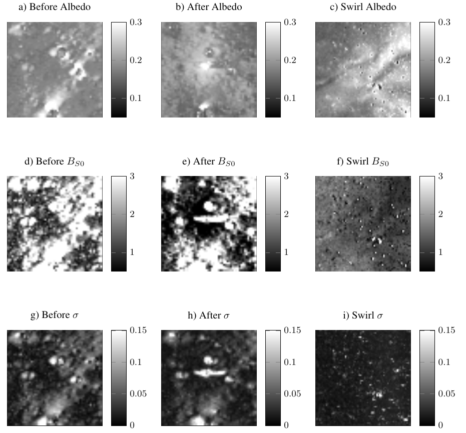
Figure 2: Maps of Hapke parameters.

Figure 3: Distribution of BS0 for the landing site after the landing and the Reiner Gamma swirl.
4. Conclusion
The landing of the Chang’e 5 rover on the Moon has changed the photometric properties of the surface. The albedo has increased and the shadow hiding opposition effect is less strong such that the phase curve has become flatter. This is generally the case for higher albedos but the reduction is nonetheless significantly even below the value expected for the brighter highlands [3]. Similarly, swirls show a reduced opposition effect. A physical explanation could be that the porosity of the regolith is reduced by fast-streaming gas from the landing rocket jet and from a passing comet, respectively (see [5]).
References
[1] B. Hapke (2012). Theory of reflectance and emittance spectroscopy, Cambridge.
[2] M.S. Robinson et al. (2010). Space science reviews, 150(1):81–124.
[3] H. Sato et al. (2014). JGR Planets, 119(8):1775–1805.
[4] Y.I. Velikodsky et al. (2016). Icarus, 275:1–15.
[5] V.V. Shevchenko (1993). Astronomy Reports, 37:314–319.
[6] J. Laura et al. (2022). URL https://doi.org/10.5281/zenodo.6329951.
[7] F. Scholten et al. (2012). JGR Planets, 117, E00H17.
[8] A. Grumpe et al. (2014). Advances in Space Research, 53(12):1735–1767.
[9] J. Salvatier et al. (2016). PeerJ Computer Science, 2:e55.
[10] A. Gelman et al. (1995). Bayesian Data Analysis, Chapman and Hall/CRC.
How to cite: Hess, M., Wöhler, C., and Qiao, L.: Photometric Modelling for Chang’e 5 Landing Site and Reiner Gamma Swirl, Europlanet Science Congress 2022, Granada, Spain, 18–23 Sep 2022, EPSC2022-147, https://doi.org/10.5194/epsc2022-147, 2022.
Introduction: Several future missions to the Moon will be devoted to robotic and human explorations in search for ice deposits and other resourses. Ground Penetrating Radar (GPR) is considered a fundamental geophysical instrument to detect water ice inside the regolith and to map the distribution of the volatiles in the lunar polar regions. The success of GPR survey relies on the capability to discriminate between dry and ice-saturated regolith or to detect lenses of relatively pure water ice. To reach this goal an intense laboratory activity is required to characterize the radar response of the lunar regolith as a function of mineralogical composition and different physical conditions (e.g., compactions, temperature, ice content). Here, we present new dielectric measurements of lunar regolith simulants in a broad range of frequencies and for different soil porosities, to improve the interpretation of radar data collected on the Moon. Such measurements have been carried out in the framework of the PrIN INAF “MELODY” (Moon multisEnsor and LabOratory Data analysis) research project, which is devoted to combining past and present lunar data to improve our knowledge on the lunar surface and shallow subsurface properties.
Laboratory measurements: GPR measurements allow one to retrieve signal wave velocity and attenuation in the lunar subsurface [1]. Such parameters are related to complex dielectric permittivity and magnetic permeability, from which some chemical-physical properties of the lunar soil and rocks can be inferred. We apply dielectric spectroscopy techniques for two pairs of commercially available, certified lunar soil analogues (Exolith Lab, 2021a, 2021b) [2, 3] to characterize the radar response of the regolith as a function of mineralogical composition and different physical conditions (e.g., temperature, porosity, and ice content). The investigation of these analogues helps us understand the most reliable lunar soil. Such analogues reproduce the composition of both lunar maria and highlands. The maria analogues are LMS-1D (particle size < 0 – 30 μm) and LMS-1 particle size < 0.04 – 300 μm). The highlands soil simulants are LHS-1D (particle size < 0.04 – 35 μm) and LHS-1 (particle size < 0.04 – 400 μm). The analogues mineralogy are reported in Tab. 1 and Tab. 2.
The measurements are performed at room temperature in the frequency range 100 kHz to 3 GHz, using a Vector Network Analyzer VNA (Agilent E5071C). The VNA ultimately provides the the electromagnetic parameters of the simulant through the Nicholson-Ross-Weir algorithm (NRW) [4]. This method allows one to retrieve both complex dielectric permittivity and magnetic permeability; however due to the negligeble magnetic properties of the samples, here only the dielectric permittivity is reported. Measurements are performend with a coaxial probe line characterized by a multiwire shield cage. Regolith analogues were first oven-dried at 105°C for 24 hours to remove residual water; then the samples are inserted in the teflon cage and different compaction are obtained through a vibration plate.
Results and future work: Fig. 1 (a and b) report the real and imaginary parts of the dielectric permittivity as a function of frequency for the Maria simulant having the smallest particle size range. Fig. 2 (a and b) illustrates the same parameters for the highland simulant. Note that for the two samples a different range of compaction is obtained. The real part of permittivity is frequency independent and decreases with increasing porosity because of the air trapped in the pores, as expected. For lunar maria it ranges from 1.8 to 2.2 (𝜙 from 70% to 60%), while the highland simulant shows higher values between 2.3 and 2.9 (𝜙 from 56% to 44%). Re- garding the imaginary part, it does not show a dependency on porosity, while it shows the same trends at every compaction over the frequency range for both simulants. The next step of the project will be the characterization of the dielectric behaviour of the simulants in a broad range of temperatures (200K – 373K).
Acknowledgements: We acknowledge support from the research project: “Moon multisEnsor and LabOratory Data analYsis (MELODY)” (PI: Dr. Federico Tosi), selected in November 2020 in the framework of the PrIN INAF (RIC) 2019 call.

References: [1] Jol, Harry M., ed. Ground penetrating radar theory and applications. elsevier, 2008. [2] Exolith Labs, U. of C.F LMS-1 Lunar Mare Simulant Spec Sheet (2021). [3] Exolith Lab, U. of C.F LHS-1 Lunar Highland Simulant Spec Sheet (2021). [4] Nicolson, A. M., & Ross, G. F. (1970). Measurement of the intrinsic properties of materials by time-domain techniques. IEEE Transactions on instrumentation and measurement, 19(4), 377-382.
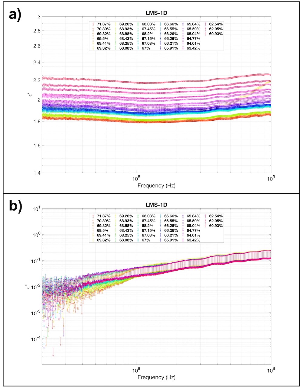
Figure 1: Real (a) and Imaginary (b) part of the permittivity as function of frequency of sample LMS-1D at varying compaction.
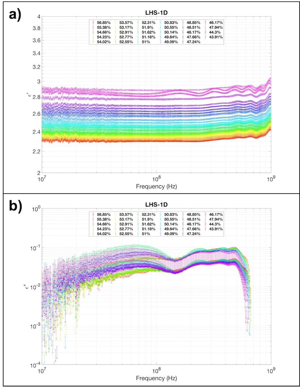
Figure 2: Real (a) and Imaginary (b) part of the permittivity as function of frequency of sample LHS-1D at varying compaction.

Table 1: Mineralogy of lunar Highlands analogues LHS-1 and LHS-1D.

Table 2: Mineralogy of lunar Maria analogues LMS-1 and LMS-1D
How to cite: Martella, C. H., Cosciotti, B., Lauro, S. E., Mattei, E., Tosi, F., and Pettinelli, E.: Dielectric measurements of lunar soil analogues at different compactions within the Melody project., Europlanet Science Congress 2022, Granada, Spain, 18–23 Sep 2022, EPSC2022-243, https://doi.org/10.5194/epsc2022-243, 2022.
This study investigates the lunar plasma environment when embedded within Earth's magnetotail. We use data from 10 years of tail crossings by the Acceleration, Reconnection, Turbulence, and Electrodynamics of the Moon's Interaction with the Sun (ARTEMIS) spacecraft in orbit around the Moon. We separate the plasma environments by magnetosheath-like, magnetotail lobe-like, and plasma sheet-like conditions. Our findings highlight that the lobe-like plasma is associated with low densities and a strong magnetic field, while the plasma sheet is characterized by higher densities and a weaker magnetic field. These regions are flanked by the fast, predominantly tailward flows of the terrestrial magnetosheath. During a single lunar crossing, however, the magnetotail displays a wide range of variability, with transient features—including reconnection events—intermixed between periods of lobe-like or sheet-like conditions. We compare and contrast the Moon's local magnetotail plasma to the environments near various outer-planet moons. In doing so, we find that properties of the ambient lunar plasma are, at times, unique to the terrestrial magnetotail, while at others, may resemble those near the Jovian, Saturnian, and Neptunian moons. These findings highlight the complementary role of the ARTEMIS mission in providing a deeper understanding of the plasma interactions of the outer-planet moons.
How to cite: Liuzzo, L., Poppe, A., and Halekas, J.: A statistical study of the Moon's magnetotail plasma environment, Europlanet Science Congress 2022, Granada, Spain, 18–23 Sep 2022, EPSC2022-291, https://doi.org/10.5194/epsc2022-291, 2022.
Introduction:
Analyses of samples returned by the Apollo Program have provided fundamental insights into the origin-history of the Earth-Moon system and how planets and solar systems work. Several special samples that were collected or preserved in unique containers or environments (e.g., Core Sample Vacuum Container (CSVC), frozen samples) have remained unexamined by standard or advanced analytical approaches. The Apollo Next Generation Sample Analysis (ANGSA) initiative was designed to examine a subset of these samples. The initiative was purposely designed to function as a participating scientist program for these samples, and as a preparation for new sample return missions from the Moon (e.g., Artemis) with processing, preliminary examination (PE), and analyses utilizing new and advanced technologies, lunar mission observations, and post-Apollo science concepts. ANGSA links the first generations of lunar explorers (Apollo) with future generations of lunar explorers (Artemis) [1-4].
Progress and Results:
Teamwork for gas extraction from CSVC 73001: To extract any potential gas phase from the CSVC, the European Space Agency (ESA) designed, built, tested, and delivered to JSC a CSVC piercing tool. To collect-store the gas phase, WUStL designed, built, and delivered to JSC a gas manifold system. Together these tools were used to open and sample the CSVC. Preliminary analyses of these gases are being carried out at UNM (Z. Sharp) and WUStL (R. Parai), which will determine whether a lunar component can be detected in the gas.
Extrusion of 73001: Following extraction of gas, the lower part of the double drive tube (73001) was imaged (µXCT, multi-spectral imaging), extruded, dissected, sieved, and examined (Pass 1 and 2). Pass 3 will remain unsieved and will be a target for PE by early career ANGSA scientists-engineers. ANGSA team members participated in the PE of 73002.
Frozen samples: The cold curation facility for processing Apollo 17 frozen samples was approved in mid-December 2021. These samples were processed and allocated in early 2022. Studies are advancing to define differences in preservation of (a) volatiles between frozen and unfrozen samples; (b) thermoluminescence kinetics in lunar samples [e.g., 5]; and (c) chronology.
Stratigraphy of 73001-73002: The stratigraphy of the double drive tube has been examined by multiple approaches. For 73001-73002, the stratigraphy was documented by µXCT imaging [6], reflectance properties [7,8], IS/FeO [8], major, minor, and trace element geochemistry [9,10], grain size/modal proportions [8,11,12], and continuous thin sections [13].
µXCT imaging of lithic fragments: Lithic fragments >4 mm in size were removed from the double drive tube during sampling passes 1-2 (73001-73002); from unsieved Pass 3 > 1cm fragments were removed. µXCT images of hundreds of these lithic fragments were produced. Fragments include a variety of breccias (some with a significant number of spherical glasses), high-Ti basalts with different cooling histories, a variety of “lower-Ti” basalts, and unique lithologies presumably derived from the South Massif. The ANGSA lithic analysis group is carrying out collaborative studies of these fragments [6,14].
Less than 1mm lithic fragments: During processing of Passes 1 and 2 from the double drive tube, samples were sieved into > 1 mm and < 1 mm size fractions. The < 1 mm size fractions were further sieved into 1000-500, 500-250, 250-150, 150-90, 90-20, and <20µm size fractions for selected intervals. In addition to determining modes of each size fraction within the stratigraphy, lithic fragments were also classified and documented. Impact melt rocks and breccias were abundant. Igneous lithologies include ferroan anorthosites, Mg-suite, “felsites”, low-Ti basalts, pyroclastic glasses, and a variety of high-Ti basalts [11,12,15]. Observations (e.g., volatiles, stable isotopes, organics, cosmogenic radionuclides, space weathering) were placed within the context of core stratigraphy [e.g., 16-21].
References: [1] Shearer et al. (2020) 51st LPSC abst.#1181 [2] Shearer (2008) Presentation to CAPTEM. [3] Shearer et al. (2019) 50th LPSC abst. #1412. [4] G. Lofgren (2007) personal communication. [5] Sehlke et al (2022) 53rd LPSC abst. #1267.[6] Zeigler et al. (2022) 53rd LPSC abst.#2890. [7] Sun et al. (2022) 53rd LPSC abst. #1890. [8] Morris et al. (2022) 53rd LPSC abst. #1849. [9] Neuman et al. (2022) 53rd LPSC abst.#1389. [10] Valenciano et al. (2022) 53rd LPSC abst.#2869. [11] Simon et al. (2022) 53rd LPSC abst.#2211. [12] Cato et al. (2022) 53rd LPSC abst.#2215. [13] Bell et al. (2022) 53rd LPSC abst.#1947. [14] Yen et al (2022) 53rd LPSC abst.#1547. [15] Valencia et al. (2022) 53rd LPSC abst#2608. [16] Cano et al. (2021) AGU Fall Meeting abst.; [17] Gargano et al. (2022) 53rd LPSC abst#2450 . [18] Recchuiti et al (2022) 53rd LPSC abst.#2193. [19] Elsila et al. (2022) 53rd LPSC abst.# 1212. [20] Welten et al. (2022) 53rd LPSC abst.#2389. [21] McFadden et al. (2022) 53rd LPSC abst. #1539.
How to cite: Shearer, C. and Zeigler, R. and the ANGSA Science Team: Using an analog lunar sample return mission to grow a lunar sample community and prepare for human return to the Moon’s surface. An update on the progress of the ANGSA initiative., Europlanet Science Congress 2022, Granada, Spain, 18–23 Sep 2022, EPSC2022-747, https://doi.org/10.5194/epsc2022-747, 2022.
- Introduction
When solar wind hits the lunar surface, a fraction of it is reflected back from the Moon instead of being absorbed by its surface. Evidence of neutral hydrogen atoms [1] and solar wind protons [2] being reflected from the surface are provided by numerous studies; however, no measurements of negative ions have been done so far. It is unknown whether or not a significant negative ion population exists near the lunar surface. The Negative Ions at the Lunar Surface (NILS) instrument, the first-ever dedicated negative ion instrument flown beyond the Earth, will address this question. NILS is being developed at the Swedish Institute for Space Physics for the Chinese Chang’E-6 sample return mission. Chang’E-6 is expected to launch in 2024 and will soft-land on the lunar far-side at approximately 41°S and 180°E. NILS will operate at least 30 minutes after the landing to achieve its main science objective. NILS operations will end with the lift-off of the sample return module.
- Main science objective
Negative ions are a not yet observed plasma component at the Moon. NILS’s main objective is to detect negative ions emitted from the lunar surface as a result of the interaction with solar wind and establish the upper limits for their fluxes. That requires NILS to distinguish and resolve the energy distributions of scattered H- and sputtered lunar negative ions, as well as to coarsely resolve different mass groups. The overarching scientific question is to estimate the importance of negative ions for space-surface interactions and environments of planetary bodies with surface-bound exospheres.
- Instrument design
NILS is the 9th generation of the SWIM family [3], a series of compact, adaptive, and capable mass spectrometers analysing ions, electrons or energetic neutral atoms at the sub-keV energy range. NILS combines a compact electrostatic analyser and a time-of-flight cell to measure the energy per charge and the mass per charge of incident ions. An additional deflection system consisting of two cylindrical electrodes allows for a one-dimensional 160° scanning of the viewing direction. NILS instantaneously records negative ions and electrons from a single direction and requires electrostatic scanning to change the viewing direction. Negative ions and electrons can be separated by an electron suppression system placed between the deflection system and the first-order focusing 127° long cylindrical electrostatic analyser. The latter is equipped with micro serrations on the outer electrode to maximize suppression of UV photons and scattered particles.
Prior to entering the time-of-flight cell, ions are post-accelerated by a -400V potential improving the sensor detection efficiency. The time-of-flight start signal is generated by a channel electron multiplier, which detects the secondary electrons generated when that particle is interacting at grazing incidence with a tungsten single crystal start surface. After the reflection on the tungsten surface, the particle travels to a stop surface, where a second secondary electron is generated that then subsequently is detected by a second channel electron multiplier, providing the time-of-flight stop signal. The time difference between the start and stop signals combined with the energy setting of the electrostatic analyser allows determining the mass per charge of the particle.
- References
[1] M. Wieser, S. Barabash, Y. Futaana, M. Holmström, A. Bhardwaj, R. Sridharan, M. B. Dhanya, A. Schaufelberger, P. Wurz, and K. Asamura. First observation of a mini-magnetosphere above a lunar magnetic anomaly using energetic neutral atoms. Geophys. Res. Lett., 37(5), 03 2010.
[2] Y. Saito, S. Yokota, T. Tanaka, K. Asamura, M. N. Nishino, M. Fujimoto, H. Tsunakawa, H. Shibuya, M. Matsushima, H. Shimizu, F. Takahashi, T. Mukai, and T. Terasawa. Solar wind proton reflection at the lunar surface: Low energy ion measurement by map-pace onboard selene (kaguya). Geophys. Res. Lett., 35, 12 2008.
[3] M. Wieser and S. Barabash. A family for miniature, easily reconfigurable particle sensors for space plasma measurements. Journal of Geophysical Research: Space Physics, 2016
How to cite: Canu-Blot, R., Wieser, M., and Barabash, S.: The Negative Ions at the Lunar Surface (NILS): first dedicated negative ion instrument on the Chang’E-6 mission to the Moon., Europlanet Science Congress 2022, Granada, Spain, 18–23 Sep 2022, EPSC2022-992, https://doi.org/10.5194/epsc2022-992, 2022.
TP4 | Mars Surface and Interior
Introduction: Mars is a primary destination to search for signs of life and probing the subsurface is a key element in this search. Access to the Martian subsurface, under most altered layers, is needed to understand the nature, timing and duration of alteration and sedimentation processes on Mars, as well as habitability conditions. For such a reason, ExoMars rover mission includes a drill to collect subsurface samples and has a complex payload able to conduct detailed investigations of composition, search for organics, and recognize indicators of past or extant life[1]. The drill is a critical element of the mission which will explore and collect samples down to 2 m of depth. An essential part of the payload is Ma_MISS (Mars Multispectral Imager for Subsurface Studies) experiment hosted by the drill system[2,3]. Ma_MISS is a Visible and Near Infrared miniaturized spectrometer with an optical head inside the drill tip capable of observing the borehole from where samples are collected.
Ma_MISS instrument description: Ma_MISS miniaturized spectrometer is hosted inside the drill system of the ExoMars rover and will characterize the mineralogy and stratigraphy of the excavated borehole wall at different depths (up to 2 m).
|
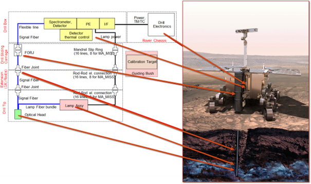
Ma_MISS is a modular instrument, and it consists of two main parts: (i) the spectrometer with the PE located outside of the drilling tool, and (ii) the Optical Head (OH) and fibers located inside the drill itself (Fig.1). The Drill consists of a main rod and three additional rods to reach a maximum depth of 2 m. The drill tip also has the Ma_MISS OH with a sapphire window to observe the borehole wall. All the rods are equipped with optical fibers to transmit light and signal. Ma_MISS is equipped with a light source of 5W and the illumination spot is about 1 mm at a focal distance of about 0.6 mm. The reflected light is collected through a 120 μm spot. The spectrometer observes a single point on the borehole wall and, using the drill movements, can build up images of the target. By combining several column and ring observations, Ma_MISS allows the reconstruction of a complete image of the borehole wall (Fig.2). Ma_MISS spectral characteristics and fine spatial resolution enable the in situ investigation of rocks, prior the sample collection, that will be manipulated and crushed for further analysis by the analytical laboratory. Thus, Ma_MISS is the instrument that will closely investigate the mineralogical characteristics of Mars subsurface material in its original geologic context.
|
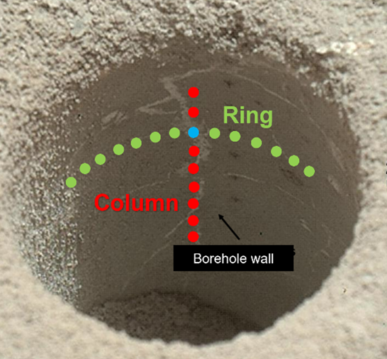
What mineralogy is expected in the subsurface ? Ma_MISS will investigate deeper into the subsurface than prior rover missions. Viking and Phoenix landers scooped materials from the upper few centimeters for compositional analysis. The MER excavated trenches up to 11 cm deep[4] and collected data with the alpha-particle x-ray spectrometer and Mossbauer instruments. The MERs [5] grounded up to 9 mm deep and revealed coatings enriched in S, Cl, Zn and Ni and iron oxides on outer rock surfaces. The MER data from the subsurface show that those soils had high ferric sulfate contents or silica contents, likely signaling an influence from volcanic or hydrothermal processes[6,7]. Mars Science Laboratory (MSL) drilled several holes into the Martian surface demostraing differences between the surface and the subsurface, as shown in the colors of the excavated fines, mainly linked with the oxidation state of the materials[8]. Most interesting is the fact that well preserved organic material was discovered at Pahrump Hills , even with the very harsh surface conditions, suggesting even better preservation may be possible farther beneath the Martian surface[9].
Differently from the previous missions, the drill and Ma_MISS measurements will be the deepest compositional measurements made on Mars. Ma_MISS is able to detect compositional gradients with depth, changes in type and abundance of minerals, weathering fronts or rinds, and diagenetic veins or nodules. The spectral range of Ma_MISS is optimal to detect changes in the occurrence and crystal chemistry of olivines and pyroxenes as well as Fe(II)/Fe(III) in silicates, oxides, and salts. There may be changes in these redox sensitive minerals with depth that record different environments. Furthermore, changes in the hydration state of materials can be also detected. For Oxia, the study of the subsurface could provide information on depositional regimes in zones not too far from the delta deposits, using the granulometric variation with dept.This will help to reconstruct the paleoenvironments that have characterized Oxia Planum.
In addition, at sufficient concentrations, organic molecules will also be detectable [10]: depending on the kind of organic, Ma_MISSis capable to detect their presence even when a 1 wt.% in the mixture, as verified by specific tests in the laboratory using the Ma_MISS breadboard. Spectroscopic measurements on these mineral/organic mixtures are useful to understand how the Ma_MISS instrument can detect traces of organic intimately mixed with minerals.
Conclusion: Ma_MISS will reconstruct the 3-D images of the borehole excavated by the ExoMars drill and will acquire spectra of the subsurface layers from which the sample will be collected. The calibration and tests performed with the flight model demonstrate the ability of the instrument in detecting most of the spectral signatures expected in Martian subsurface, including those due to the presence of possible salts and organics.
Acknowledgments. This work is fully funded and supported by the Italian Space Agency (ASI) [Grant ASI-INAF n. 2017-48-H.0].
References. [1] Vago et al. (2017) Astrobiology 17, 471–510. [2] De Sanctis, M. C. et al. (2017) Astrobiology, 17(6–7). [3] De Sanctis et al. (2022) PSJ in press. [4] Sullivan, R., et al.. (2011), J. Geophys. Res., 116, E02006; [5] Gorevan et al., (2003), J. Geophys. Res., 108, 8068; [6] Gellert, R and Yen, A.S, (2019) Remote Compositional Analysis, 10.1017/9781316888872, (555-572); [7] Morris et al., (2019), Remote Compositional Analysis, 10.1017/9781316888872, (538-554); [8] Abbey et al., (2020), Icarus, /doi.org/10.1016/j.icarus.2020.113885. [9] Eigenbrode et al., 2018, Science, doi/10.1126/science.aas9185, [10] Ferrari et al., 2022. In preparation.
How to cite: De Sanctis, M. C., Altieri, F., De Angelis, S., Ferrari, M., Frigeri, A., Fonte, S., Ammannito, E., Brossier, J., Giardino, M., Apuzzo, A., costa, N., and rossi, L.: Ma_MISS: a powerful tool for exploring the Martian subsurface, Europlanet Science Congress 2022, Granada, Spain, 18–23 Sep 2022, EPSC2022-104, https://doi.org/10.5194/epsc2022-104, 2022.
Introduction: Fresh Shallow Valleys (FSVs) are relatively undegraded dominantly mid-latitude valleys and valley networks that are generally shallowly incised (<20 m). into mantle substrate [1]. They are primarily of Hesperian to Amazonian age and are found in the mid-latitudes (30-50° N/S). The primary interpretation is formation through surface runoff of snowmelt, although a sub-ice hypothesis has been suggested for some crater-interior FSVs [2]. Exit-breach craters (EBCs), or pollywog craters, are relatively fresh craters primarily in the 1-7 km diameter range with no contributing drainage beyond the rim, and one or more exit valleys [1, 3].
Observations: Systematic ArcGIS mapping of FSVs and EBCs was conducted in the southern mid-latitudes using the Murray Lab CTX mosaic at a 1:100,000 scale. Of 1668 craters mapped as possible EBCs, 435 of these were designated as firm detections by having evident rim incision, visibly incised valleys, and no exterior contributing drainage. FSVs were mapped only exterior to craters, although many interior crater rims are dissected by FSV-like valleys. A total of 7276 FSVs were mapped averaging 7.2 km in length. Fig. 1a shows the latitudinal distribution of FSVs and EBCs and Fig. 1b the size distribution of EBCs. FSVs and EBCs have similar latitudinal distribution. To assess the possible hydrology of FSVs and EBCs, topographic relationships were analyzed using CTX and HRSC DTMs.
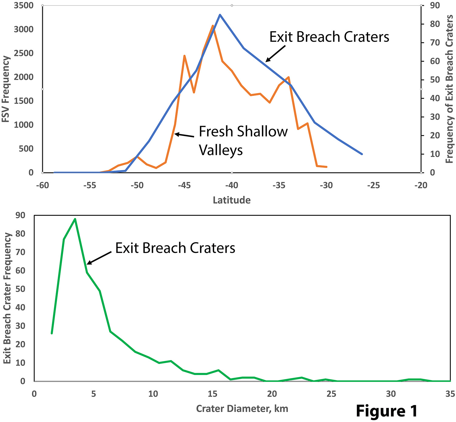
The most deeply incised FSVs occur across divides in settings connecting intercrater basins or connecting intercrater basins to crater interiors (Figs. 2 and 3). Fig. 2 shows FSVs on the northeast exterior rim of a 46 km diameter crater at 44.3°S, 165.2°W. The interior of the crater is indicated by “#”. A ~1 km wide valley leads from the exterior crater rim northward (white arrow). Three ~150m wide FSVs (“a”, “b” & “c”) extend from the valley axis east and northeast with gradients of about 0.04. Each of these FSVs breach the eastern rim of the north-trending valley. The depression on the exterior crater rim at “x” is drained by at least five east-trending FSVs that incise a low ejecta ridge.
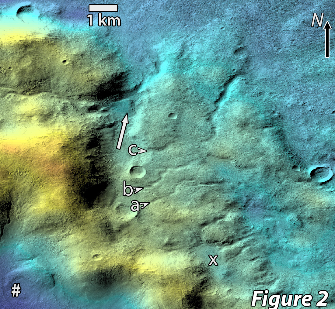
Fig. 3 is centered on the southeastern exterior rim of the same crater. Part of the crater rim is at “#”. The exterior rim depression “d” was drained by two FSVs, one of which extends to the rim depression at “a”. This basin in turn was drained by the FSV shown at the arrow, which incises through an exterior rim ridge at “b”. The lowpoint of the southern rim of basin “a” is at “c”, which is about 30 m lower that the elevation of the FSV rim breach at “b”.
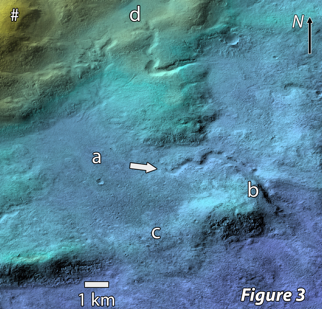
Most EBCs have a single exit breach, but some have multiple breaches. Fig. 4 shows an exit breach crater at 120.56°W, 43.88°S with a minimum of three exit breaches and possibly as many as seven.
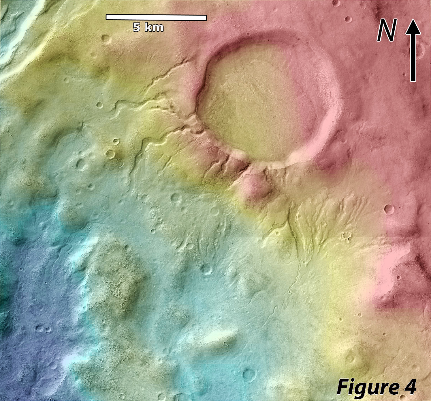
Analysis and Conclusions:
FSV morphology is distinct from typical terrestrial and the older martian valley networks: 1) they are mostly shallowly incised; 2) they are often isolated features; 3) depth of dissection is <20 m unless they cross divides; 4) many display sinuous planforms; 5) FSVs commonly connect basins across topographic divides, often through multiple breaches and extending to nearly the basin floor in both basins; 6) FSV divide breaches often do not occur at the topographic lowpoints between basins. The exit channels of EBCs are morphologically like FSVs and often accordantly drain into FSVs. As such, FSVs and EBCs probably share a common hydrological environment. Because of their relative youthfulness and mid-latitude environment, FSVs have been suggested to be fed from snowmelt, indicating a post-Noachian environment that could support occasional surface temperatures exceeding freezing [1, 4]. However, melting of seasonal or meter-scale snow cover does not readily account for FSVs breaching divides unless one of the basins overflowed.
EBCs are likewise enigmatic. Filling of craters by groundwater influx to overflow conditions has been suggested [1,3], but many EBCs occur on divides, as in Fig. 4. Filling of craters to overflow from precipitation (presumably melting of snow and ice) could lead to catastrophic breach incision [3, 5]. We suggest a common hydrological scenario for both FSVs and EBCs as resulting from episodic melting of a >100 m deep snow/ice cover accompanied by flow through basal ice tunnels (R-channels) [6]. Estimation of FSV discharge from gradient and meander wavelength using the approach of [7] suggests values <100 cumecs. In terrestrial glacial settings, divide-crossing subglacial channels generally create eskers due to bedload aggradation. On Mars, FSVs may be largely incised into fine-grained mid-latitude mantle deposits, so little coarse bedload would be entrained and channel beds might erode through scour or melting rather than aggrading. Divides breached by FSVs seldom exceed 50 m of relief relative to adjoining basins, suggesting 150-250 m of ice cover might be sufficient to support R-channel flows. Whether wider braided/anastomosing FSVs [1] can form beneath ice is uncertain. Perennial water might exist below the ice cover in the relatively undegraded EBCs, causing overflow either from surface ice accumulation or melt percolating through the ice cap. If flow rates overspilling EBCs are modest, rim incision may be restricted to removing the fine-grained mid-latitude mantle materials. The lack of large EBCs probably reflects insufficient ice cover to create overflow.
References: [1] Wilson, S. A. et al., (2016), JGR Planets 121, 1667-94, [2] Hobley, D. E. J. et al., (2014), JGR Planets 119, 128-53. [3] Warren, A. O. et al., (2021), EPSL 554, doi:/10.1016/j.epsl.2020.116671. [4] Howard, A. D., Moore, J. M., (2011), JGR 116, E05003. [5] Goudge, T. A. et al., (2021), Nature 597, 645-49. [6] Walder, J. S., (2010), J. Glaciol. 56, 1079-85. [7] Howard, A. D. et al., (2008), LPSC 39, Abs. 1629.
How to cite: Howard, A., Wilson, S., and Moore, J.: Fresh Shallow Valleys and Exit Breach Mid-Latitude Craters: Formation Below a Thick Ice Cover, Europlanet Science Congress 2022, Granada, Spain, 18–23 Sep 2022, EPSC2022-180, https://doi.org/10.5194/epsc2022-180, 2022.
MarsSI (“Mars Système d’Information”, french for Mars Information System) is a platform and service to explore, process and retrieve data from orbiters. https://marssi.univ-lyon1.fr/MarsSI. This poster aim to help user to understand and use this service.
Introduction
Geological investigations of planetary surfaces require the combination of orbital datasets. Missions being often multiple-instruments platforms from multiple space agencies, the quantity of data available increased quickly. MarsSI is a platform designed to explore, process and retrieve Mars orbital data. It was certified in 2017 as french national Research Infrastructure by the Centre National de la Recherche Scientifique (CNRS) as part of the Planetary Surface Portal (PSUP, <https://psup.cnrs.fr/>).
As of 2021, it indexes the optical (visible, multi and hyper-spectral) data from the recent orbiter missions, and allow to request the creation of Digital Elevation Models on demand. The focus, as highlighted by figure 1 is to allow the user to browse and request ”ready-to-use” products in regards of calibration, refinements and georeferencing. The user will be able to visualize and interpret the data in GIS or remote sensing software.
MarsSI
MarsSI aim to provide both a way to explore and use data from space agencies archives, such as the Planetary Data System (PDS), but also run data processing pipelines to make this data ready for analysis and as a shared, collaborative, repository. This allows a scientific user to more easily access data from their raw level and proceed to surface investigations and interpretation.
Explore datasets
MarsSI access is done through a web application. This interface, completely updated in 2021, provide a map where product footprints can be visualized over various backgrounds (MOLA, Themis, CTX) to put data in context. Instruments, and if needed, their acquisition modes, are available as layers to display.
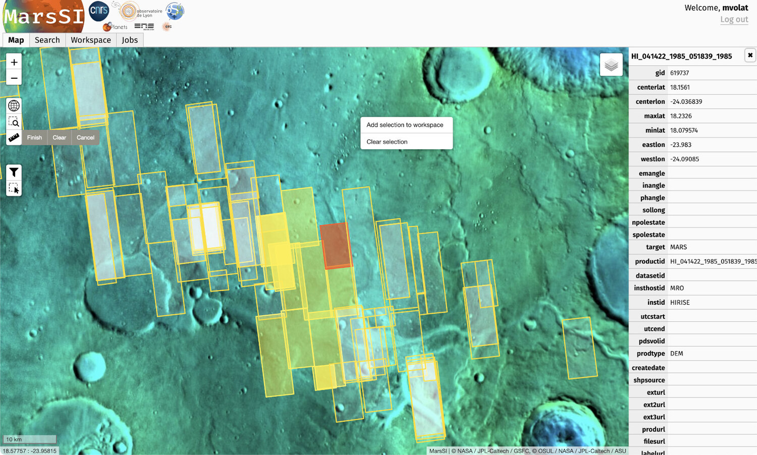
In this part of the interface, the user will be able to select products of interest and add them to a workspace summarizing the data he need to use.
Until now, MarsSI has focused on the most recent missions (ODY, MEX, MRO) optical datasets (visible, NIR, hyperspectral) and derived products.
Pipelines
Pipelines execution is done on demand, and requested from the workspace pane of the interface. Each type of product (based on instrument) has a specific pipeline defined. The pipelines are designed to be fully automated, run on MarsSI's computing cluster, and to not require any user input. This is done partially to ease the usage of the service, to avoid managing and storing multiple versions with slight differences that would make references to products more complex.
Basic pipelines operate to bring products to calibration and map projection (and georeferencing) steps. Those pipelines are usually based on ISIS (https://isis.astrogeology.usgs.gov/) for visible spectrum images.
More advanced pipelines allows to calibrate and create spectral parameter maps from CRISM hyperspectral cubes using the CRISM Analysis Toolkit (CAT, https://pds-geosciences.wustl.edu/missions/mro/crism.htm), and another to create stereophotogrammetry-derived DEMs from the CTX and HiRISE datasets (in complement of the pre-processed DEM datasets available) based on Ames StereoPipeline (https://ti.arc.nasa.gov/tech/asr/groups/intelligent-robotics/ngt/stereo/). One notable feature is that the DEM datasets are computed from the optical imagery datasets, showing all the stereo pairs deemed feasibles (based on overlap calculation and having a difference of incidence angle of at least 10°).
Documentation
MarsSI is documented through a wiki that provide information on both the platform usage and the products.
Conclusion
MarsSI (https://marssi.univ-lyon1.fr) aims to offer a way to the scientific communities to easily explore and perform the necessary processing steps for the data needed in their projects. MarsSI itself has seen superficial and architectural changes since it was recognized as part of a french national service, and aim to extend its datasets range in the future. Use of the service require registration that is free for a non-commercial usage.
Ackowledgements
MarsSI is a national Research Infrastructure, recognised as such by the French Ministry of Higher Education and Research. It was supported by the Programme National de Planétologie (PNP) of CNRS/INSU, co-funded by CNES. It was initialy supported by the European Research Council under the European Union’s Seventh Framework Program (FP7/2007-2013)/ERC Grant agreement No.280168.
How to cite: Volat, M. and Quantin-Nataf, C.: MarsSI: Martian surface data processing service, Europlanet Science Congress 2022, Granada, Spain, 18–23 Sep 2022, EPSC2022-213, https://doi.org/10.5194/epsc2022-213, 2022.
Introduction: Despite the large amount of information from orbital and in situ missions, the characteristics and evolution of Mars’ early climate are still widely debated among the scientific community. Morphological evidence dating back to about 3-4 billion years ago, such as valley networks [1], and the presence of several hydrated minerals [2] seem to indicate that Mars once had a “warm and wet” climate with abundant water on the surface and possibly even an ocean in the northern lowlands [1-3]. These conditions eventually changed through time leading up to the hyperarid and cold planet we observe today.
The area of Meridiani Planum (MP), located SW of Arabia Terra, is well known for retaining multiple evidence of past aqueous activity [4] and a varied hydrated mineralogy [5]. The majority of the terrains exposed in MP formed at the Noachian-Hesperian boundary [6], that is between two important epochs of Mars: the Noachian (4.1-3.7 Ga), where most of the evidence for water is found, and the Hesperian (3.7-3.0 Ga), which is characterized by increasingly water-limited conditions. Constraining the potential water environment at the NH boundary is fundamental to understand Mars’ early climate and its evolution.
In this study, we select 7 craters in Northern MP (figure 1) showing evidence of NH sediment infillings with hydrated materials (e.g., clays and sulfates) to assess in detail the stratigraphic sequence of the mineralogical units and understand their origin and diagenetic history. The craters are roughly aligned SE to NW following the general slope of the area from the highlands to the lowlands. If Mars experienced a “warm and wet” period, MP would represent a transition zone between the subaerial alteration environment of the highlands and the subaqueous environment of the Martian ocean. Therefore, the area would be easily affected by climatic changes whose evidence should be retained in its sedimentary sequences.
We show here some preliminary results from 2 out of the 7 craters selected for the study:
1) a 15-km-wide crater named Mikumi, centered at Lat. 2.45°N, Lon. 359.96°E;
2) an 18-km-wide unnamed crater centered at Lat. 4.25°N, Lon. 2.85°E.

Figure 1: THEMIS daytime image of Meridiani Planum. Selected craters are evidenced with points. Name (if given) and coordinates of the center for each crater are also indicated with a label. Most of the craters are unnamed. The arrows indicate the two craters described in this abstract.
Datasets and methods: We investigate the mineralogy of the craters’ terrains through CRISM [7] hyperspectral data cubes mainly in the range 1.0-2.6 μm. This interval retains part of the key spectral features of primary rock-forming minerals, which constitute the Martian crust, and of most minerals produced by secondary processes such as aqueous circulation and alteration (e.g., clays and sulfates). MOLA, THEMIS, CTX and HiRISE data are then used for morpho-stratigraphy and camera imaging.
Results: Two types of clays (smectites) with different Fe/Mg content, polyhydrated sulfates and monohydrated sulfates are observed in both craters (figure 2). Fe/Mg-clay spectra (e.g., nontronite and saponite) show absorptions at around 1.4, 1.9 and 2.3 μm with additional overtones at 2.4 μm. The exact position of the 2.3 μm feature depends on the relative Fe/Mg content in the clay mineral. We find some areas with clays richer in iron (e.g., nontronite), showing this feature centered at 2.305 μm, and clays richer in magnesium (e.g., saponite) where the absorption is centered at 2.310-2.315 μm. In Mikumi crater, polyhydrated sulfates (Mg sulfate) and monohydrated sulfates (kieserite) are detected stratigraphically below the clay-bearing layer. For the unnamed crater, the stratigraphic relationship of the units is still to be investigated.
Figure 2: (top) CRISM spectra of detected mineralogy. Fe/Mg clays (smectites) are from Mikumi crater, mono and polyhydrated sulfates are from the Unnamed crater. The spectra are extracted from FRT0000BEF5 and FRT00009B5A TRR datasets respectively. (bottom) Laboratory spectra of clays and sulfates from the CRISM spectral library [8] (Mg Sulfate ID: CJB366; Kieserite ID: F1CC15; Saponite ID: LASA51; Nontronite ID: NCJB26).
Discussion and conclusions: Clays and sulfates on Mars appear to have formed at different times and under different climatic conditions [9]. Clays are usually associated to Noachian terrains and may have formed under alkaline conditions in a “warm and wet” ancient Mars, whereas sulfates are typically associated to Hesperian surfaces and may have formed under a dryer and more acidic environment. Therefore, sulfates are expected to be found stratigraphically on top of clays, as they should have formed later in Mars’ history. However, this distinction between a clay-rich Noachian and a sulfate-rich Hesperian oversimplifies the history of the aqueous chemistry and climate of Mars especially near the NH boundary.
Our analysis suggests a stratigraphic sequence with interleaving clays and sulfates at the NH boundary. Similar stratigraphic sequences have also been observed in other areas of MP (Southern MP) by [5]. In the case of [5], a clay-bearing layer is overlain by other sulfates, generating a sulfate/clay/sulfate stratigraphic sequence. All this argues is in favor of several distinct climatic episodes pacing the NH climatic transition.
The results obtained so far will be enriched by further analysis of these areas along with a thorough investigation of the remaining 5 craters selected.
Acknowledgments: Featured CRISM data were downloaded from the Planetary Data System (PDS). This project is partially supported by Europlanet RI20-24 GMAP project.
References: [1] M. H. Carr and J. W. Head (2010) Earth and Planet. Sci. Lett., 293, 185-203. [2] B. L. Ehlmann and C. S. Edwards (2014) Annu. Rev. Earth Planet. Sci., 42, 291-315. [3] R. A. Craddock and A. D. Howard (2002) JGR, 107 (E11), 5111. [4] R. M. E. Williams et al. (2017) GRL, 44, 1669-1678. [5] J. Flahaut et al. (2015) Icarus, 248, 269-288. [6] B. M. Hynek et al. (2002) JGR, 107 (E10), 5088. [7] S. Murchie et al. (2007) JGR, 112 (E5), E05S03. [8] C. E. Viviano-Beck et al. (2015) MRO CRISM Type Spectra Library, NASA Planetary Data System. https://crismtypespectra.rsl.wustl.edu [9] J. P. Bibring et al. (2006) Science, 312, 400-404.
How to cite: Baschetti, B., Massironi, M., Carli, C., Altieri, F., and Frigeri, A.: Clay and sulfate-bearing terrains in Northern Meridiani Planum, Mars: constraining the characteristics of Mars’ early climate at the Noachian-Hesperian boundary, Europlanet Science Congress 2022, Granada, Spain, 18–23 Sep 2022, EPSC2022-222, https://doi.org/10.5194/epsc2022-222, 2022.
The Curiosity rover of the Mars Science Laboratory has been exploring since mid-2021 the lower sulfate unit of Mount Sharp in the Gale crater. This unit, first described from orbital observations as showing spectral signatures of hydrated sulfate minerals [1], has recently been revealed to record a major paleoenvironmental and climatic transition during the Hesperian-Noachian transition, with the onset of alternating wet and dry conditions before a complete aridification of Martian conditions [2]. Before the current campaign, this unit was mainly studied using remote observations (e.g., [2, 3]), but Curiosity has now entered this major interval allowing to precisely study the rock record leading to this major climatic event.
Since the rover left the Glen Torridon area (aka the clay-bearing unit, Fig. 1), the Curiosity rover entered the sulfate-bearing unit (~Sol 3100, mid-2021; Fig. 1) and traversed sedimentary series mainly composed of fine to coarse sandstones. While no clear facies change or sharp contact has been observed when entering the sulfate-bearing unit, these levels differ from the previously observed terrains in Gale by an increased occurrence of nodular features with a strong sulfate geochemical signature [4, 5], polygonal ridges [4], or even halite detections [6]. Otherwise, the sedimentary structures and grain-size are continuous across the upper members of the Carolyn Shoemaker formation and into the overlying Mirador formation, indicating a likely continuity in the continental settings for most of these deposits.
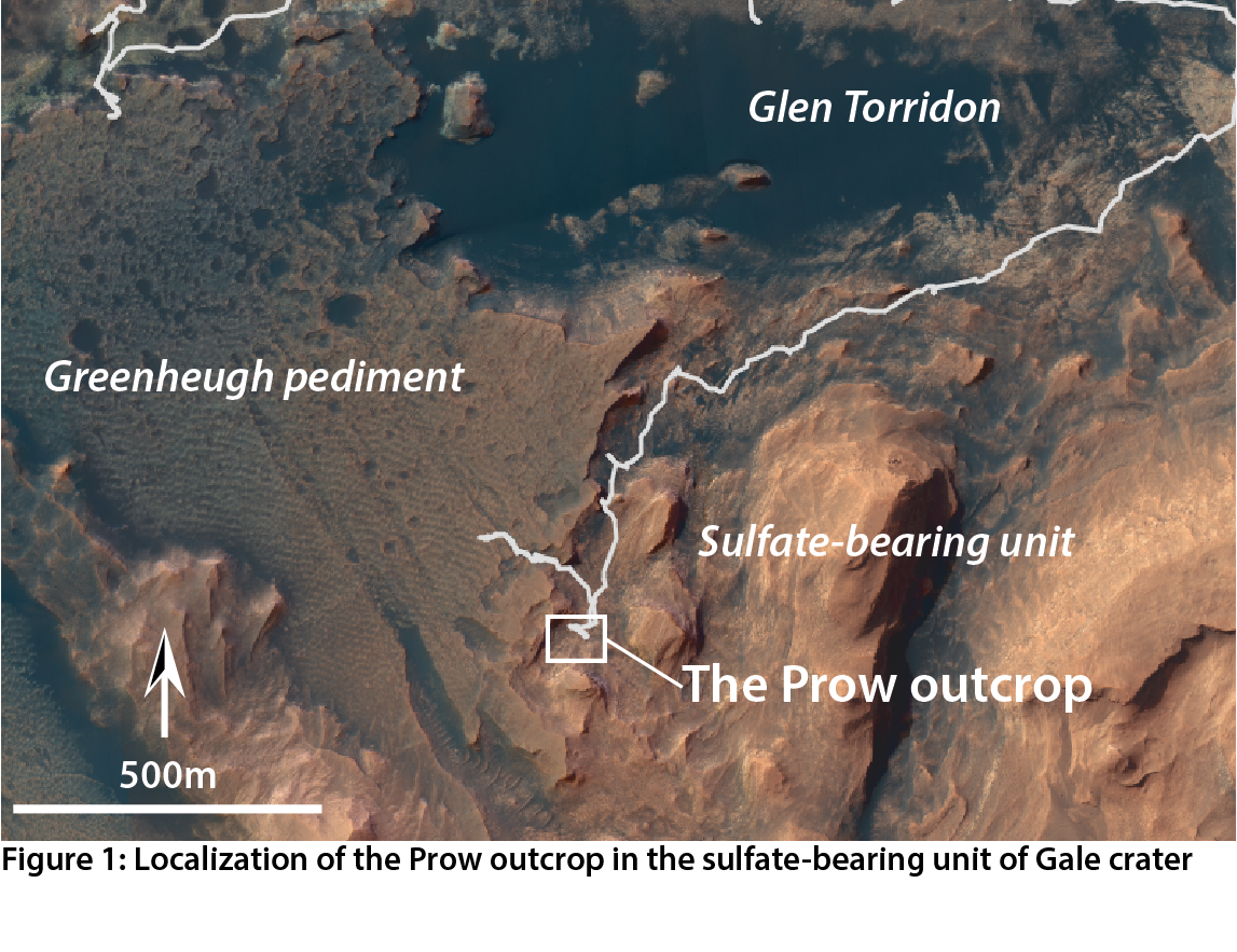
Such structures are notably well visible at the Prow locality, a major outcrop situated in the Contigo member of the Mirador formation, just below the Greenheugh pediment (Fig. 1). This outcrop has been reached and studied in January and February 2022, between sols 3349 and 3379. Using ~3200 mid- and close-range images from the Navigation and Mast cameras (Navcam, Mastcam), we used structure-from-motion photogrammetry to reconstruct a Digital Outcrop Model (following the method described in [7]) of the Prow locality and its vicinity (Fig. 2). This DOM covers an area of about 1000m². Two small excerpts of this DOM are explorable online on the Sketchfab platform at https://skfb.ly/o8DJZ and https://skfb.ly/otpLW. The DOM allows us to visualize and characterize several sets of meter- to centimeter-scale sedimentary structures, over about 30 meters of lateral continuity, either using on-screen visualization, or integrated within a Virtual Reality environment.
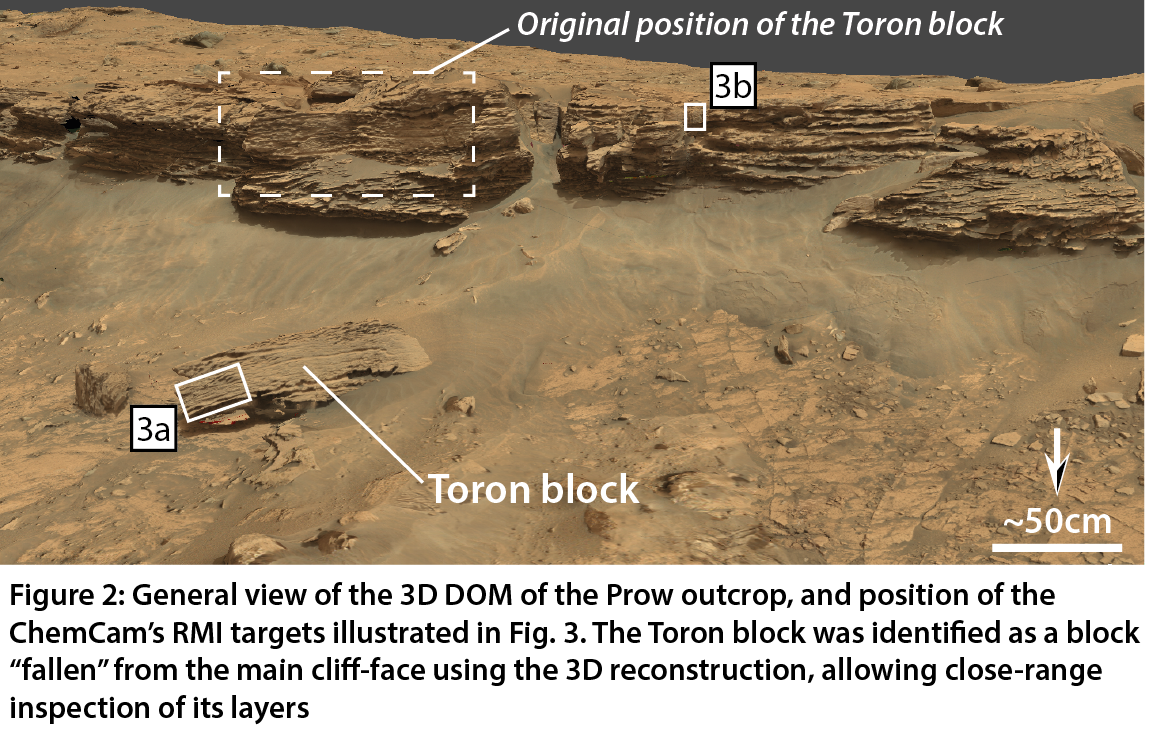
The DOM reconstruction has been helpful in determining the targets of interest during the Prow exploration by Curiosity. One particular benefit has been to identify the Toron block (Fig. 2) as a fallen piece of the main outcrop, allowing us to perform very close-range observations of the outcrop’s cliff-face (e.g., Fig. 3a) without actually putting the rover too close to the actual rock-face. The interest of using such 3D reconstruction notably lies in the ability to characterize the spatial distribution of the multi-scale structures observed at the Prow, but also to study the spatial distribution (and potential variations) of the geochemical composition of these layered sandstones as seen by the ChemCam instrument. We also take advantage of the high-resolution micro-images provided by the Remote Micro-Imager subsystem of the ChemCam instrument (with a field of view of 20 mrad per frame, resolving grains under the silt at close range) to study the facies (grain-size, micro-structures) of the different sandstone beds cropping out at this locality (Fig. 3).
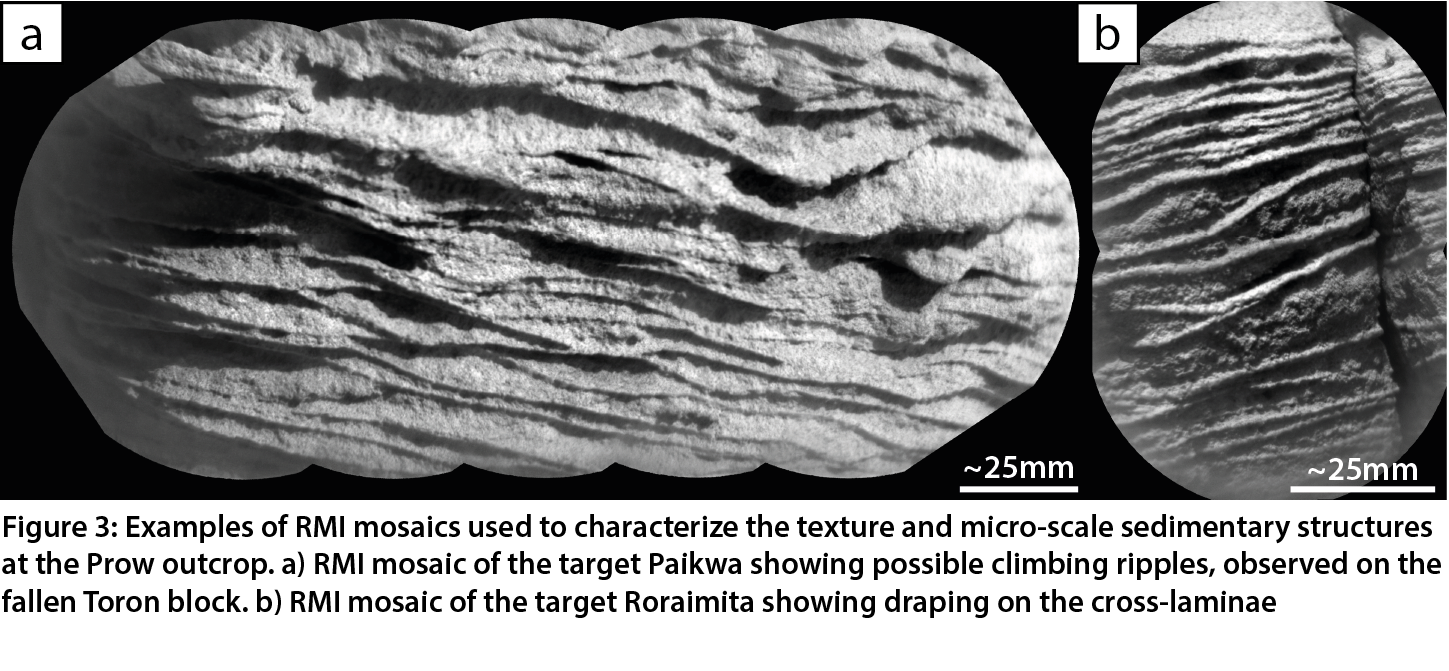
At the Prow, we characterize several sets of sedimentary structures such as (but not limited to) meter-scale cross-stratifications, cm-scale symmetric ripples but also probable climbing ripples (Fig. 3a). These structures, mostly indicating a direction of transport toward the NW (similar to what is observed in underlying Glen Torridon area), denotates sustained aqueous conditions compatible with a fluvial setting. We also observe in some place at the Prow, and notably in the upper layers, mm-scale fine-grained draping (Fig. 3b) deposited at the surface of (cross-)stratifications, reminiscent of flaser bedding on Earth. These fine muddy levels indicate recurrent intervals of low-energy deposition in-between higher-energy periods. Put together, these elements help us to characterize sustained aqueous conditions in a dynamic setting of combined flow and wave action at the time the sediments were deposited (e.g., [8]), helping us to determine probable mixed fluvio-aeolian settings around the critical climatic transition observed within this sulfate-bearing unit characterized by alternating wet and dry conditions.
References: [1] Miliken et al., 2010, Geophys. Res. Lett. 37, L04201; [2] Rapin et al., 2021, Geology 49; [3] Caravaca et al., 2021, Remote Sensing, 13(20), 4068; [4] Rapin et al., 2022, EPSC, this meeting; [5] Schieber et al., 2022, LPSC, Abstract #1304; [6] Meslin et al., 2022, LPSC, Abstract #2492; [7] Caravaca et al., 2020, Planet. Space Science 182, 104808 ; [8] Gupta et al., 2022, ESPC, this meeting.
How to cite: Caravaca, G., Le Mouélic, S., Gupta, S., Mangold, N., Rapin, W., Schieber, J., Le Deit, L., Gasnault, O., and Lanza, N. L.: The Prow outcrop: an “open catalog” of multiscale 3D fluvial sedimentary structures in the lower sulfate unit of Gale crater (Mars), Europlanet Science Congress 2022, Granada, Spain, 18–23 Sep 2022, EPSC2022-336, https://doi.org/10.5194/epsc2022-336, 2022.
Fluvial landforms on Mars are important because they indicate past liquid water. The landforms can provide information about past environmental and climate conditions and the potential for past life. Ancient fluvial sediment transport fluxes have been estimated for several channels on Mars. However, it is also important to understand the differences between sediment transport on Earth and Mars. Fluxes can differ significantly due to gravity, sediment density, lack of ecology and the possible presence of ice. Only when we understand the effects of such differences on sediment fluxes, we can apply and adapt knowledge of fluvial geomorphology on Earth to the surface of Mars. Additionally, such understanding will greatly improve the use of Earth analogues.
In this study, we isolate the effects of gravity on fluvial sediment transport with a 1D model of a simple static channel and a 2D depth-averaged numerical hydro-geomorphological model of a growing delta. The results show that sediment transport on Mars is more efficient than on Earth for the same water discharge, sediment distribution, and channel geometry. The 1D results show that mainly fine sediment is transported more efficiently on Mars, because the effect of gravity is stronger on suspended transport compared to bedload transport and bigger grains travel in suspension on Mars compared to Earth for the same boundary conditions. Because gravity affects fine and coarse sediment fractions differently, we also expect differences in geomorphology due to different ratios of sediment fractions and disparities in sediment sorting. We are exploring these morphological effects in our 2D delta model. Our preliminary results suggest that the lower gravity on Mars results in faster-growing deltas with lower slopes and wider channels. These results suggest that unexpected differences with Earth might also occur in the delta stratigraphy, which is important to realise when drilling for sediment samples in the search for biosignatures.
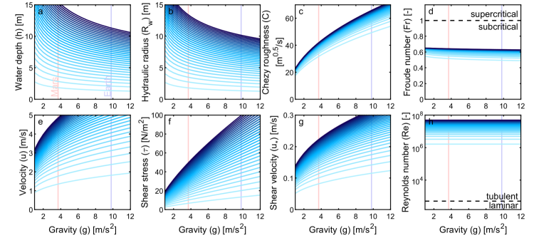
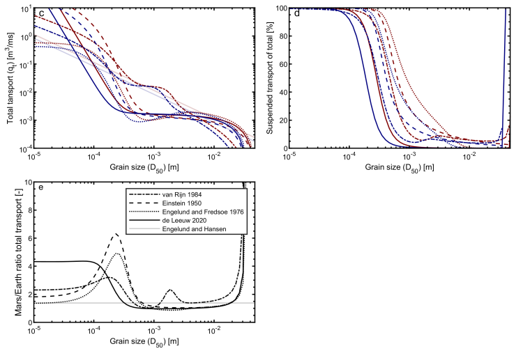
How to cite: Braat, L. and Lamb, M. P.: Isolated effects of gravity on sediment fluxes and delta morphology, Europlanet Science Congress 2022, Granada, Spain, 18–23 Sep 2022, EPSC2022-356, https://doi.org/10.5194/epsc2022-356, 2022.
Introduction: On Earth, sharp drops in temperature can cause ground cemented by ice to contract, forming surficial cracks (Figure 1a) that can join to form polygonal patterns. These polygons show no elevation difference between their margins and centres, and are called here flat-centred polygons (FCPs). Water and/or sand [1, 2, 3] can infill the troughs and freeze, forming ice or sand wedges. These grow seasonally, uplifting polygon margins above the centres, forming low-centred polygons (LCPs). When wedges degrade, the elevation of the margins decreases below that of the centre, forming high-centred polygons (HCPs).
The martian mid-latitudes exhibit similar polygons (Figure 1b), currently thought to form by ground thermal-contraction [4]. Whereas debate ensues over the nature of trough infill, recent work provided evidence for ice wedges in Utopia Planitia [5] – with implications for liquid water stability and subsurface water ice availability.
Here we study variations in polygon distribution/morphology in relationship with different geological units in UP (Figure 2) and Arcadia Planitia (AP; Figure 3), where polygonised units have been reported [6]. Our study seeks to understand: 1. how the substrate nature favoured/inhibited the formation and/or preservation of ground ice, and 2. whether polygon characteristics (e.g. morphology, spatial density) can give insights into geological properties of their substrate.
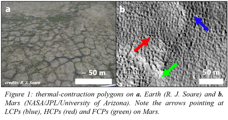
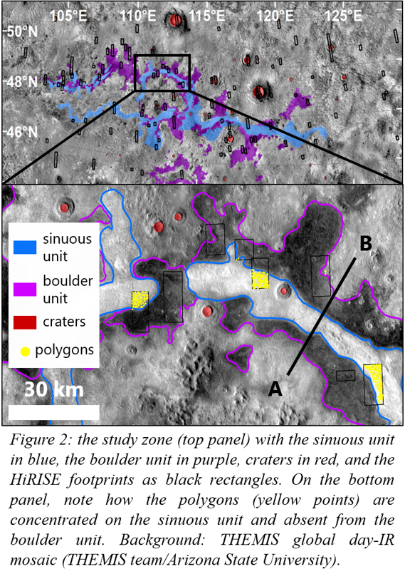
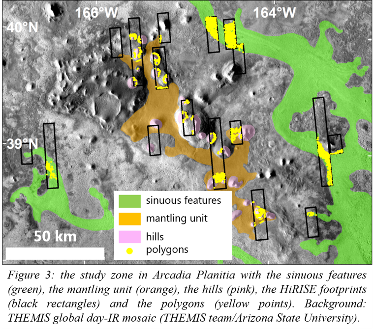
Methods: In UP (Figure 2a) we mapped polygons (5-25 m scale) on 104 images from the High-Resolution Imaging Experiment (HiRISE, 25-50 cm/pixel) – 55 from [5] and 49 new ones. We used a grid-based mapping approach [7]: we gridded images into 500x500 m squares, and in each square the presence of a given polygon type was noted when at least five specimens were present. We mapped the extent of three units: a sinuous unit, a boulder unit, and craters (Figure 2) with imagery from the Thermal Emission Imaging System (THEMIS), the Context Camera (CTX) and HiRISE. We also produced a topographic cross-section of contacts between the sinuous and the boulder units (Figure 2b) with data from the Mars Orbital Laser Altimeter (MOLA).
For each unit we calculated three parameters: 1. the percentage of polygonised squares (%pol), 2. the percentage of polygonised squares containing solely FCPs (%FCPs), and 3. the ratio number of squares containing LCPs / number of squares containing HCPs (LCP/HCP). We suggest that these parameters reflect properties of the substrate: 1. its cementation by ice, 2. its capacity to grow ice wedges (i.e. massive ground ice), and 3. its capacity to preserve ground ice.
We used the same approach on 18 HiRISE images in AP, where we mapped the extent of three units based on [6]: hills, a mantling unit, and sinuous features.
Results: We display and compare results for each unit in Table 1. In UP, topography and cross-section data (Figures 2b & 4) show that the boulder unit is at a lower elevation than the sinuous unit and also the surrounding terrains. In AP, hills exhibit FCPs around their central mound (Figure 5a); sinuous features bear FCPs, HCPs and what we interpret as degraded HCPs (Figure 5b); and the mantling unit bears few polygons, but is mostly covered in extensive brain terrain and linear ridges [6] (Figure 5c).
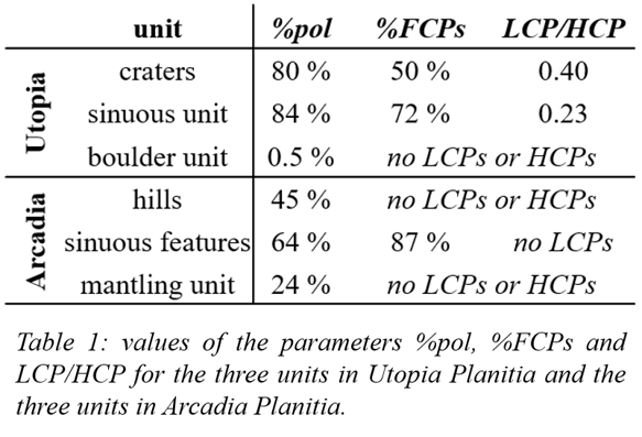
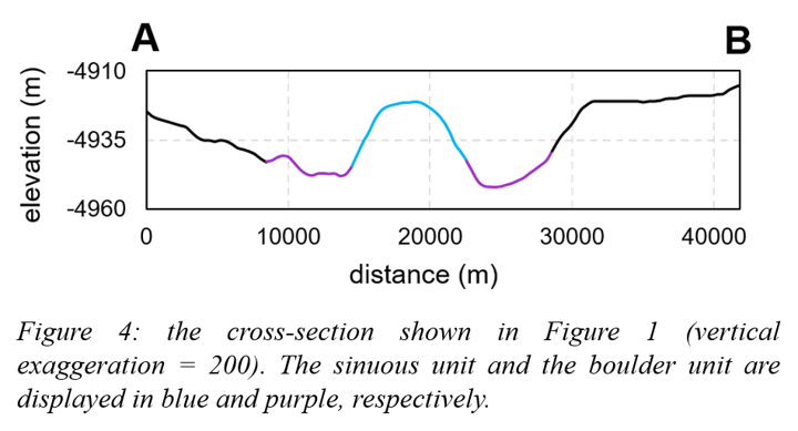
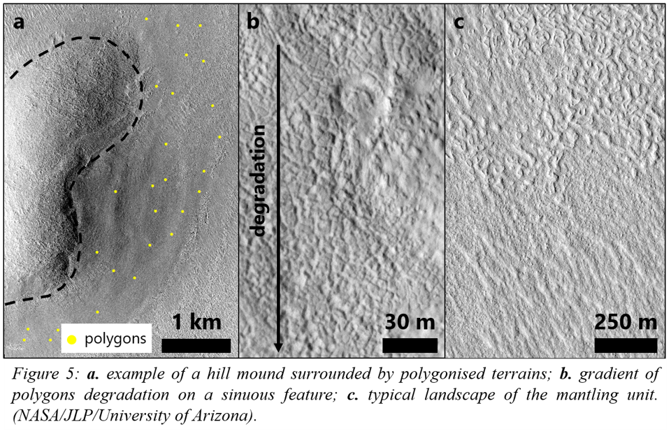
Discussion:
Utopia Planitia: The material infilling craters is highly polygonised (high %pol), show evidence of past ice wedge formation (low %FCPs), and preserved more ice wedges (high LCP/HCP). Therefore, it should be porous and ice-rich [8, 9], suggesting sediment that underwent ice deposition events. This could have been enhanced by a cold-trap effect [5, 10].
The boulder unit exhibits boulders, fractured rocks and nearly no polygons - suggesting a massive material hindering ground ice emplacement and thus ground cracking. The sinuous unit is higher in elevation and highly polygonised (high %pol), showing evidence of ice wedge activity and of LCP preservation – but less than craters (higher %FCPs and lower LCP/HCP). Substrate here should thus favour massive ice emplacement and preservation - but to a lesser extent than craters. Moreover, the study zone is located at the terminus of Hrad Vallis, a valley thought to have conveyed both lava and mudflows [11]. Therefore, we suggest that the boulder unit is an ancient low-viscosity lava flow [12], superposed by the sinuous unit which is a more recent mudflow, both having been conveyed by Hrad Vallis.
Comparison Utopia/Arcadia Planitia: Despite both being at similar latitudes, the polygonisation in AP is different to that in UP: AP exhibits degraded HCPs and no LCPs. Therefore, we suggest that AP underwent an ancient period of ice (or sand) wedge aggradation, which stopped and was followed by landform degradation.
Conclusions: We have shown that the morphology of thermal-contraction polygons can give insights into substrate properties, and help define its geological origin. In UP, it allowed us to infer the origins for both the boulder and the sinuous units, consistently with the regional geological context. In future work we will explore the timing of polygonisation in the mid-latitudes: did this process start and stop earlier in AP than in UP? or did the ice wedge activity last longer in UP? how old are the units bearing polygons, and how long does it take to erode them? These points could have important implications concerning the timing of liquid water stability on Mars.
References: [1] Péwé T. L. (1959) AJS 257, 545-552. [2] Lachenbruch A. H. (1962) GSA Special Paper 70. vol. 69. [3] Black R. (1976) Quaternary Research 6(1), 3-26. [4] Mellon M. T. (1997) JGR 102 (E11), 25,617-25,628. [5] Soare R. J. et al. (2021) Icarus 358, 114208. [6] Hibbard S. M. et al. (2021) Icarus 359, 114298. [7] Ramsdale J. D. et al. (2017) PSS 140, 49-61. [8] Lefort A. et al. (2010) Icarus 205, 259-268. [9] Levy J. S. et al. (2009) JGR 114, E01007. [10] Conway S. J. et al. (2012) Icarus 220, 174-193. [11] Hamilton C. W. et al. (2018) JGR Planets 123, 1484-1510. [12] Hopper J. P. and Leverington D. W. (2014) Geomorphology 207, 93-113.
How to cite: Philippe, M., J. Conway, S., J. Soare, R., and E. Mc Keown, L.: Relationship between the density/type of thermal-contraction polygons and the geology of the substrate at the Martian mid-latitudes., Europlanet Science Congress 2022, Granada, Spain, 18–23 Sep 2022, EPSC2022-425, https://doi.org/10.5194/epsc2022-425, 2022.
Abstract
Northwestern part of Terra Cimmeria displays a wide range of fluvial, lacustrine and glaciofluvial geomorphological features, indicative of presence of liquid water in this area early in the Martian history. These features were previously mapped as part of global studies, but not in relation to the area itself. Here we present our reconstruction of hydrologically correct model of northwestern Terra Cimmeria based on algorithm assisted mapping exercise of unprecedented precision. Based on our findings we are able to contextualize the geomorphological specifics of individual subbasins within the framework of Late Noachian Icy Highlands model and subsequent climatic transition towards the dry and cold state of the Amazonian period.
Physiographic Characteristic
Terra Cimmeria is an extensive region of the Martian southern highlands. Its northwestern portion (Northwestern Terra Cimmeria, NWTC) lies in the equatorial area of the planet and likely did so even before the Tharsis-induced true polar wander event (Bouley et al., 2016). It is nested between the volcanic province of Hesperia Planum to the southwest and the Utopia highland-lowland boundary to the north (Skinner and Tanaka, 2007). In the setting of the disputed Arabia Level ocean shoreline (Sholes et. al, 2021 and references therein) NWTC would stand out as the longest peninsula on Mars. The surface of NWTC is dominated by the Late Noachian highland unit with „undifferentiated impact, volcanic, fluvial and basin material“ (Tanaka et al., 2014). There are several open-basin lakes as mapped by Fassett and Head (2008), craters in different stages of degradation, and numerous valley networks which dissect the terrain (Carr, 1995; Hynek et al., 2010; Alemanno et al., 2018) and few on which terminate as deltaic deposits previously mapped by Achille and Hynek (2010). The variety and density of geomorphological features whose formation is tied to the presence of volatiles suggests a rich history of fluvial, lacustrine, and glaciofluvial activity and importantly fluvially dominated erosion and deposition. We incorporated available imagery and previously derived datasets in our algorithm assisted mapping exercise in order to contextualize the putative sources of the valley carving runoff within the local climatic background.
Methodology
NWTC valley networks were mapped several times in different level of detail starting with Carr (1995) who based his mapping on Viking imagery. This initial campaign was followed by Hynek et al. (2010) who utilized THEMIS daytime IR imagery and MOLA DEM and later by Alemanno et al. (2018) who in addition to THEMIS daytime IR and MOLA DEM used the ConTeXt (CTX) camera imagery to improve their recognition capability where the forementioned datasets lacked sufficient resolution.
Our mapping is based on the high resolution global CTX image mosaic rendered at 5 m/pixel (Dickson et al., 2018), THEMIS nighttime IR dataset, and MOLA DEM with the vectorized valley network dataset of Alemanno et al. (2018) serving as a baseline. We used Whitebox GAT surface flow accumulation model with hybrid breaching-filling sink removal capability (Lindsay, 2015) to digitalize the thalwegs as well as subbasins based on MOLA DEM. The algorithm-derived thalwegs and previously mapped valley networks were used to guide and double check the manual mapping which was based strictly on the CTX and THEMIS nighttime IR mosaics. Subsequently, digitalized subbasin borders were checked against the CTX mosaic and corrected based on the underlaying terrain. Notable geomorphological features were identified and marked as point features and putative headwater areas we delineated based on the previously logged data.
Results
We mapped an area spanning more than 8✕105 km2 and reconstructed 7 main valley networks. The valley networks were divided into over 80 subbasins based on manual correction of flow accumulation model. We managed to identify and connect seemingly isolated stretches of valleys and incorporate them into their respective networks thus creating a hydrologically correct reconstruction of the area. We identified several headwater-specific geomorphic features, pingos and paleolakes.
Discussion
In Noachian NWTC was situated between the equilibrium and terminus lines of a Late Noachian Icy Highlands (LNIH) ice sheet (Fastook and Head, 2015) and as such it would favor the formation of subglacial channels fed by meltwater (Galofre et al., 2020) and accumulation of ice (Wordsworth et al., 2013; Fastook and Head, 2015). The presence of developed dentritic networks which could have been carved by glavial meltwater is proven by our mapping exercise. Head et al. (2022) proposed that the climate of Mars underwent a transitional period during which a decrease in the atmospheric pressure induced a shift from altitude dependent temperature regime typical for the Noachian period (Wordsworth et al., 2013) towards latitude dependent temperature regime of the Amazonian period. This transition would start with ablation and melting of the lower altitude icy deposits and end with desiccation of equatorial ice reservoirs – both of which are in broader sense applicable to NWTC. In the beginning of this transitional period, meltwater released during the phases of peak temperatures would return to the highland cold traps in the time between these episodes. It is therefore plausible that given the specific combination of altitude, latitude, and location of NWTC, this area could sustain active surface or near-subsurface hydrology for an extended period of time up to 106 -108 years. This is supported by the variety of geomorphic features present in NWTC, but remains to be further tested with buffered crater counting and development of conceptual and hydrological models based on the newly created datasets.
Acknowledgements
VC & YM were supported by Czech Science Foundation (#20-27624Y).
References
Carr, Michael H. (1995), doi:10.1029/95je00260; Skinner, J. A., & Tanaka, K. L. (2007), doi:10.1016/j.icarus.2006.08.013; Fassett, C. I., & Head, J. W. (2008), doi:10.1016/j.icarus.2008.06.016; Achille, G. D., & Hynek, B. M. (2010), doi:10.1038/ngeo891; Hynek, B. et al. (2010), doi:10.1029/2009je003548; Wordsworth, R et al. (2013), doi:10.1016/j.icarus.2012.09.036; Tanaka, K. L. et al. (2014), doi:10.3133/sim3292; Fastook, J. L., & Head, J. W. (2015), doi:10.1016/j.pss.2014.11.028; Bouley, S. et al. (2016), doi:10.1038/nature17171; Lindsay, J. B. (2016), doi:10.1002/hyp.10648; Alemanno, G. et al. (2018), doi:10.1029/2018ea000362; Dickson, J. et al. (2018). A Global, Blended CTX Mosaic of Mars with Vectorized Seam Mapping: A New Mosaicking Pipeline Using Principles of Non-Destructive Image Editing; Galofre, A. G. et al. (2020), doi:10.1038/s41561-020-0618-x; Sholes, S. F. et al. (2021), doi:10.1029/2020je006486
How to cite: Cuřín, V. and Markonis, Y.: Reconstruction of Northwestern Terra Cimmeria Watersheds, Europlanet Science Congress 2022, Granada, Spain, 18–23 Sep 2022, EPSC2022-549, https://doi.org/10.5194/epsc2022-549, 2022.
Introduction.
Earth's most-ancient crust has been recycled through plate tectonics processes making it unlikely that we will ever directly sample it (although, one can imagine finding ancient Earth meteorites one the Moon [1].) Mars, on the other hand, hosts ancient crustal outcrops on its surface. The uplifted massifs surrounding Argyre, Hellas, and Isidis – the three largest, well-preserved impact basins on Mars - formed in the chaotic aftermath of the basin-forming impacts due to normal faulting caused by crustal thinning from impact excavation [2]. Our goal is to understand the igneous minerals associated with uplifted massifs using the Compact Reconnaissance Imagining Spectrometer for Mars (CRISM) [3] around Argyre, Hellas, and Isidis (Fig. 1). Here, we present initial results in this effort for the north Hellas area and expect to present preliminary results for Argyre and Isidis, as well, at the conference.
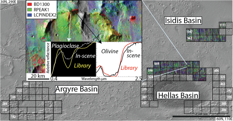
Fig. 1 Context view of the study area. Squares outline 5°x5° CRISM tiles. Number of tiles is 100, covering an approximate 5% of the surface. CRISM coverage is >80 % over tiled areas. Inset shows a region at the map scale of 1:250,000 with CRISM spectra of uplifted massifs compared to library spectra. In the spectral parameter combination, red is consistent with olivine, yellow with plagioclase, and blue with low-calcium pyroxene.
Methods.
CRISM Data Processing. We used CRISM multispectral mapping data (MSP) and hyperspectral mapping data (HSP). The MSP mapping strips have 19 visible to near-infrared (VNIR, 0.4-1 µm) spectral channels and 55 short-wavelength infrared (SWIR, 1-4 µm) channels, and the HSP mapping strips contain 107 VNIR channels and 154 SWIR channels. Both mapping datasets have a ground sampling distance of approximately 180 m. The set of wavelength channels contained in the MSP dataset were chosen to sample more densely in wavelengths regions known to contain absorption features of minerals likely to be detected on Mars (primary rock-forming silicates, phyllosilicates, etc. [3]). For our study, HSP data were resampled to the MSP wavetable to increase the spatial coverage. Typical coverage of the MSP+HSP dataset is ~85%, with sufficient overlap to allow for mosaicking and radiometric reconciliation. We processed these data through a custom pipeline [4] that includes initial noise filtering, photometric and atmospheric corrections [5], [6], and an empirical correction for “spectral smile” [7]. The final products of this pipeline are 5°x5° mosaic tiles with improved inter-strip variability in atmospheric residuals [8].
A typical method for condensing the information contained in a CRISM image into an interpretable form is by calculating “spectral parameters”, i.e., mathematical summations of particular characteristics of the spectra [9]. Spectral parameters can be combined into 3-band RGB images that highlight specific, thematically-related, combinations of interest. Fore example, the MAF summary product combines indexes intended to highlight mafic mineralogy: olivine (OLINDEX3), low-calcium pyroxene (LCPINDEX2), and high-calcium pyroxene (HCPINDEX2). From the CRISM mapping tiles, we constructed summary products that are well-suited for compositional mapping over large areas [10] (e.g., Fig. 1).
Compositional Mapping. Regions of interest were identified with the map tile summary products in ArcGIS followed up by detailed spectral analyses in IDL/ENVI (specialized software for analyzing hyperspectral images) with custom add-on analysis tools. Point locations of compositions, confirmed through spectral analysis, were imported back into ArcGIS and “outcrops” were mapped using summary products. We define outcrop in the context of this work as a spatially contiguous region with an internally consistent spectral signature distinct from its surroundings (e.g., Fig. 2).
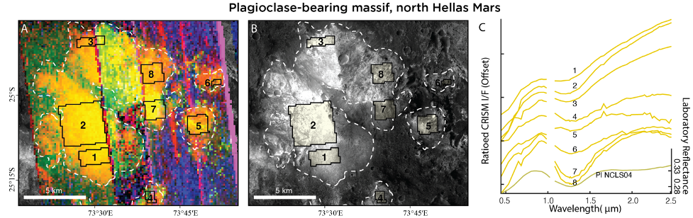
Fig. 2 Example plagioclase-bearing massif north of Hellas basin. (A) CRISM browse product (same as in Fig. 1). Yellow tones are consistent with plagioclase. Black boxes indicate 8 regions over which spectra were taken and plotted in C. (B) CTX 5 m/pixel image of the same massif as in (A). White dashed lines denote outcrops mapped in this A and B. (C) Average CRISM ratioed I/F spectra from the 8 regions indicated in A and B.
Results and Discussion.
Thus far, we have mapped 12 high-calcium pyroxene-bearing outcrops, 97 plagioclase-bearing outcrops, 128 LCP-bearing outcrops, and 129 olivine-bearing outcrops (Fig. 3). Outcrops with distinct mineralogical signatures are often observed adjacent to each other on the same massif, or on massifs in close spatial proximity (relative to the size of the massifs, ~several kilometers). We also identified Fe-, Mg-, and Al-phyllosilicate minerals associated with the massifs and, more commonly, with impact crater ejecta along the northern Hellas rim.
The number and spatial extent of plagioclase-bearing outcrops was surprising and is described in [11]. The massifs pre-date Hellas (≥ 4.1 Ga) and are situated stratigraphically above putative mantle material. The north Hellas massif outcrops may expose the remains of an ancient large igneous complex, perhaps similar to terrestrial layered mafic intrusions. Preliminary results from the Argyre and Isidis uplifted massifs will be presented at the conference and compared to those from north Hellas.
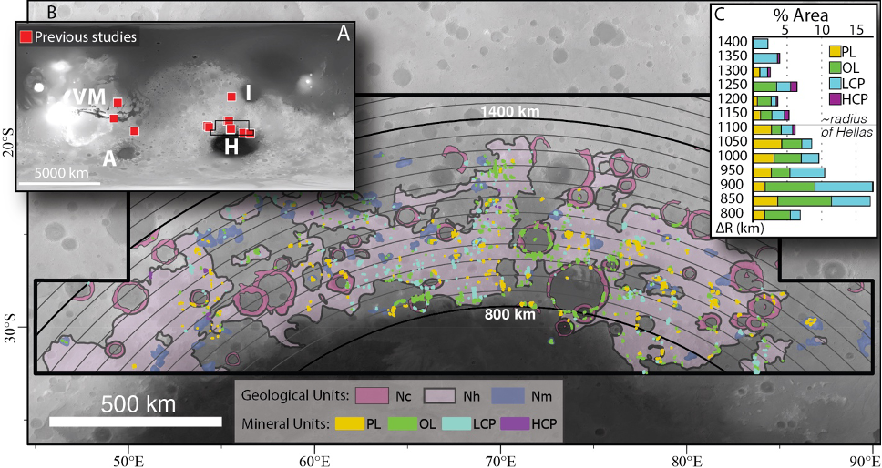
Fig. 3 Summary of detections over north Hellas. (A) Red squares indicate all locations of plagioclase-rich outcrops discovered previous to our work. (B) Context map showing all mafic mineral outcrops mapped in our study. Arcs are 50-km interval bins measured radially from the center of Hellas. Geologic units are Noachian crater (Nc), Noachian highland (Nh) and Noachian massif (Nm) from Leonard and Tanaka, 2001. (C) %Area is the area of each mineral outcrop normalized to the area of the Nc, Nh, and Nm geologic units in each radial bin. Note the concentration of detections interior to the nominal radius of Hellas, highlighting the stratigraphically low position of the outcrops.
[1] J. J. Bellucci et al. doi: 10.1016/j.epsl.2019.01.010.
[3] G. J. Leonard and K. L. Tanaka, 2001.
[4] S. L. Murchie et al. doi: 10.1029/2009je003344.
[5] F. P. Seelos and S. L. Murchie, LPSC. p. 2325, 2018.
[6] F. P. Seelos, et al., LPSC. p. 1783, 2016.
[7] F. Morgan et al., LPSC. p. 2453, 2011.
[8] F. P. Seelos et al., LPSC. p. 1438, 2011.
[9] F. P. Seelos, et al., LPSC p. 2635, 2019.
[10] C. E. Viviano‐Beck et al. doi: 10.1002/2014JE004627.
[11] C. E. Viviano et al., LPSC, p. 1485, 2020.
[12] Phillips, M. S., et al., Geology, accepted.
How to cite: Phillips, M., Viviano, C., Moersch, J., Rogers, A. D., and Seelos, F.: Mars uplifted massifs: unique and extensive samples of ancient crust., Europlanet Science Congress 2022, Granada, Spain, 18–23 Sep 2022, EPSC2022-736, https://doi.org/10.5194/epsc2022-736, 2022.
1. Introduction
Some terrestrial concretions may be analogs of Martian concretions "blueberries". They were discovered on Mars in the Meridiani Planum area (0°12′N, 357°30′E) by the Opportunity rover. The conditions for the sedimentation of Martian concretions are still unknown. They could have arisen in a similar sedimentation environment as some terrestrial concretions. Therefore, it is important to determine which Earth concretions are analogs of Martian concretions and under what conditions they were formed. This would significantly enrich knowledge about the conditions prevailing on Mars during the formation of Martian concretions, and would be an important evidence for the presence of liquid water in the history of the red planet [1], [2].
2. Concretions from Utah
Near the MDRS (Mars Desert Research Station) base in Utah, USA, sandstone concretions of Cretaceous Dakota Formation were collected. In contrast, the early Jurassic concretions in the Navajo Formation adjacent to Dakota are additionally covered with a thick layer of hematite and other iron compounds. It is known that they crystallized in layers of fine sandstone. As the sandstones were eroded, concretions fell out of them by gravity. Then it can reach to a re-crystallization on the surface of these concretions in a similar way as on the concretions from Jurassic layers of the Navajo Formation from Utah [3], [4].
|
|
|
|
|
Fig.1. A layer of Cretaceous sandstone from the Dakota Formation in Utah with concretions. The size of the visible layer with concretions of about 0.5 m.
|
|
Fig.2. Sandstone concretions of the Cretaceous sandstone of the Dakota Formation in Utah.
|
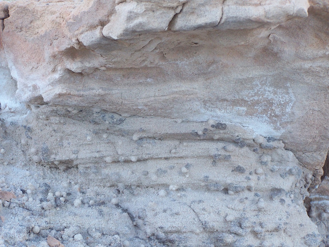

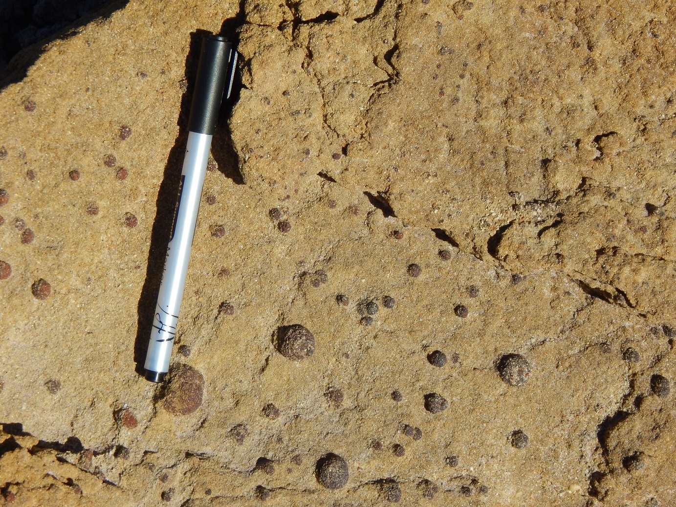
Fig.3. Surface of the Dakota Cretaceous sandstones with distinct mineralization of iron oxides.
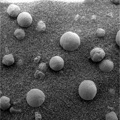
Fig.4. Image from the Microscopic Imager camera showing concretions taken by the Opportunity rover on Meridiani Planum. This image is ~3 cm across and was taken on the 15th day of Opportunity's journey (NASA Feb. 8, 2004).
Figs 1,2 show concretions in the Cretaceous layer, leached by migrating waters and re-mineralized, for which carbonates also contribute [5]. Fig. 3 shows concretions highly mineralized with iron oxides with a large proportion of hematite and goethite. When these concretions fall out by gravity, another mineralization takes place on their surface, in the case of Utah again with iron oxides, which creates a kind of glassy shell on the concretion [6].
In many publications, scientists emphasize that these concretions were formed in presence of water. Their chemical mineralization is quite complex because the water that migrates through the porous sandstones is responsible for the crystallization of these formations thanks to the dissolved chemical compounds. There is a repeated mineralization and demineralization, and therefore the chemical composition of concretions in different regions of the world may differ despite the similar origin of their formation [7], [8], [9].
3. Comparison of spectra
In our research we used the results obtained with the Mossbauer spectrometer for Martian soil with "blueberries", Fig.4, [10]. We identified the minerals likely to be present at the sample. We used appropriate spectra for these minerals from the USGS library and compared them to the infrared spectra of concretions from Utah- Fig.5.
Since the Mossbauer spectrometer does not provide information about all possible minerals because it focuses on minerals containing the Fe element, it is possible that the mineralization of Martian concretions is much richer. Jarosite and hematite discovered by the Mossbauer spectrometer fit well with the bands of the infrared spectra of the Utah concretions. Moreover, the minerals that can be recognized in the spectra of concretions from Utah are also clay minerals and gypsum. The sandstones in which this mineralization took place, of course, contain quartz, but in the short infrared range it has no spectral characteristics, therefore quartz is not visible in the spectrum.
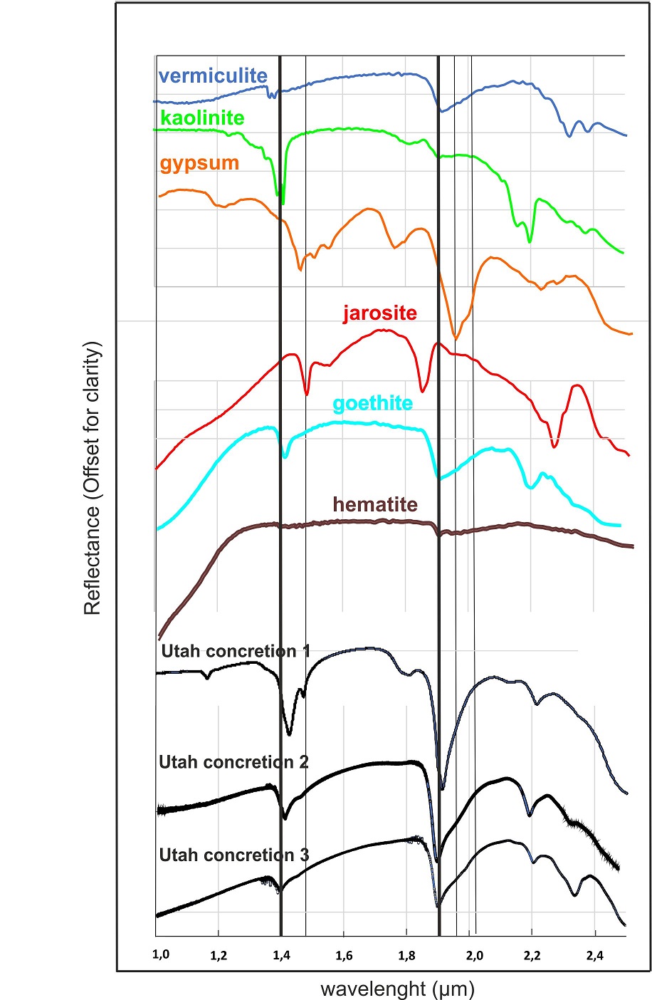
Fig.5. NIR spectra of the Cretaceous Dakota Formation in Utah (spectrometer Nicolet iS50) compared with minerals from the USGS library. The 1.4 and 1.9 µm bands reveal the influence of clay minerals and iron oxides, and additionally sulphates (gypsum and jarosite).
4. Conclusions
We found significant correlation between the Utah concretions of the Dakota Formation and those found by the Opportunity rover. A common feature of these concretions is a similar ferric sulphate mineralization. It follows that Martian and Utah concretions might have formed in an acidic environment and water was important for their formation.
References
[1] Chan, M., et al., (2005) GSA Today, 15, 8, 4-10
[2] Fan, Ch., et al., (2010) Planet. Space Sci., 58, 401–410
[3] Busigny, V., and Dauphas, N., (2007) Earth and Planet. Sci. Let., 254, 272–287
[4] Potter, S., and Chan, M., (2011) Geofluids
[5] Parry, W., (2011) Sediment. Geol., 233, 53-68
[6] Chan, M., et al., (2007) Geofluids, 7, 1–13
[7] Mika, K., et al., (2018) Geofluids of Utah, 47, 197-219
[8] Di Bella, M., et al., (2021) Minerals, 11, 460, 1-18
[9] Ray, D., et al., (2021) Planet. Space Sci., 197, 105163
[10] Klingelhofer, G., et al., (2004) Science, 306, 1740-1745
How to cite: Zalewska, N. and Czechowski, L.: Some remarks about Martian "blueberries" and spherical concretion from Utah, Europlanet Science Congress 2022, Granada, Spain, 18–23 Sep 2022, EPSC2022-737, https://doi.org/10.5194/epsc2022-737, 2022.
Introduction
Apart from the Earth, no planetary body is mapped more extensively and to such fine resolution as Mars. The increasing volume of remote sensing data means we are better equipped than ever to answer the fundamental questions about the history of the planet. However, the volume of data grows much faster than the number of scientists who can use it. Machine Learning (ML) is a powerful tool for automating the analysis of ever-increasing volumes of remote sensing data.
Aeolian bedforms exhibit varied morphologies at different scales in remote sensing imagery, therefore, automated detection is a complicated problem. Linear dune fields have been successfully characterized at regional scales using edge detection on Titan from synthetic aperture radar images [1]. Within the field of Earth observation, an edge detection algorithm has been proposed that is optimized for recognizing linear dune fields in panchromatic Landsat 8 data and digital elevation models [2]. Fingerprint minutiae extraction software designed for forensic applications has also successfully detected dune crests and their bifurcations and terminations for linear dunes in the Namib Sand Sea and Strzelecki Desert, and for Transverse Aeolian Ridges (TARs) on Mars [3].
A method for mapping aeolian ripples has been demonstrated using HiRISE imagery from Gale crater [4]. Similarly to earlier studies, this uses a two-step algorithm that segments the bedforms from the surrounding terrain and then detects the crestlines [5]. This study uses the same approach but with a segmentation step that classifies bedforms according to scale and morphology as opposed to foreground-background.
The aim of this study is to create a more general bedform detector that can be applied over larger and more texturally diverse areas of Mars. Moreover, it should perform as well as classic methods employed by geologists such as manually mapping crestlines. This will be assessed in terms of orientations and crest line maps produced but also in terms of the inferred wind regime. The secondary goal of this study is to demonstrate how ML terrain classifications designed for rover navigation can be repurposed for science.
Method
A machine learning system called the Novelty or Anomaly Hunter – HiRISE (NOAH-H) has been developed to classify terrain in HiRISE images from Oxia Planum and Mawrth Vallis according to texture. It was designed to assess terrain for rover traversability but also demonstrates great potential to be used for science [6]. Each pixel of an input HiRISE image is assigned one of 14 classes. These classes represent every type of terrain that can be found at the Oxia Planum and Mawrth Vallis landing sites, summarized in table 1. Classes 8 through to 13 are the six types of ripple morphology that are recognized by NOAH-H.
| 1 | Non-bedrock | Smooth, Featureless |
| 2 | Smooth, Lineated | |
| 3 | Textured | |
| 4 | Bedrock | Smooth |
| 5 | Textured | |
| 6 | Rugged | |
| 7 | Fractured | |
| 8 | Large Ripples | Simple form, Continuous |
| 9 | Simple form, Isolated | |
| 10 | Rectilinear form | |
| 11 | Small Ripples | Continuous |
| 12 | Non-continuous, Bedrock substrate | |
| 13 | Non-continuous, Non-bedrock substrate | |
| 14 | Other Cover | Boulder fields |
Table 1: Ontological classes used by NOAH-H. Large refers to decimeter scale features and small refers to meter scale features.
Class 9, "large simple form isolated ripples", corresponds to the larger-scale TARs in these regions and we use the NOAH-H output to segment the TARs from the surrounding terrain. Some of these classified regions contain more than one TAR, therefore the next step splits these into separate regions. Now that we can assume that every region corresponds to a single TAR, we calculate an orientation for each region using second order central image moments.
Planned Analysis
This method will be applied to HiRISE images already classified by NOAH-H in Oxia Planum. We will compare the spatial distribution and orientation of TARs using the proposed method with those measured from a study that measured 10,753 TARs by manually digitizing crestlines [8]. They will also be compared in terms of inferred wind regime and compared with a global climate model to see if they give the same conclusions. The next step to build on this work is to implement existing or new methods for the remaining 5 bedform classes detectable by NOAH-H, in order to make a more general bedform characterization method.
References: [1] Lucas A. et al. (2014) JGR, 41, 6093–6100. [2] Telfer M. W. et al. (2015) Aeolian Research, 19, 215-224. [3] Scuderi L. (2019) Aeolian Research, 39, 1-12. [4] Vaz D. A. and Silvestro S. (2014) Icarus, 230, 151-161. [5] Pina P. et al. (2004) LPS XXXV, Abstract #1621. [6] Barrett A. M. et al. (2022) Icarus, 371, 114701. [7] Canny J. (1986) IEEE TPAMI, PAMI-8, 6, 679-698. [8] Favaro E. A. et al. (2021) JGR Planets, 126, e2020JE006723.
How to cite: Bohacek, E., Barrett, A., Favaro, E., Balme, M., and Sefton-Nash, E.: Transverse Aeolian Ridges at the ExoMars Rover landing sites, Europlanet Science Congress 2022, Granada, Spain, 18–23 Sep 2022, EPSC2022-957, https://doi.org/10.5194/epsc2022-957, 2022.
TP5 | Mars Science and Exploration
Introduction:
Between March 2018 and December 2019, millions of spectra of Mars' surface and atmosphere thermal emission have been recorded in nadir geometry by TIRVIM/ACS, a thermal infrared spectrometer onboard the ExoMars Trace Gas Orbiter (TGO) [7]. From this wealth of data, we characterized in detail the thermal structure of the Martian lower atmosphere at a great variety of local times. Here we focus on the study of migrating thermal tides derived from TIRVIM observations, including during the Global Dust Event of MY34.
Observations and Methods:
We have developed an algorithm coupling line-by-line radiative transfer and optimal estimation theory to retrieve the surface temperature, the vertical profiles of the temperature between a few km and 50-55 km (2–3 Pa), and the integrated optical depth of dust and water ice clouds [3]. The retrieved temperature profiles have a vertical resolution of 10 km in the lower atmosphere and a coarser resolution of 15-20 km in the range 2–20 Pa. They were validated against thousands of co-located observations from the Mars Climate Sounder, acquired in limb viewing geometry [3].
Thermal structure and tides:
Thermal tides are planetary-scale oscillations resulting from the diurnal solar forcing of the thin Martian atmosphere. Migrating tides describe sun-synchronous modes propagating westward with the sun. The diurnal mode has one maximum and one minimum per day and a zonal wavenumber of one; the semi-diurnal mode has two maxima and two minima per day and a zonal wavenumber of two; etc. One of the main advantage of TGO’s orbit is that the local time of TIRVIM nadir observations drifts by 13 minutes earlier each sol. After 54 sols, or 25-35° of Ls, a full coverage of the daily cycle is achieved, allowing to separate between diurnal and seasonal temperature variations. This is clearly an asset to study thermal tides compared to previous studies, mostly based on 2-4 AM and 2-4 PM temperatures obtained from sun-synchronous orbiters [1,4,6,9].
An example of the zonally-averaged temperature retrieved from TIRVIM at 30 Pa in the period March 13 - April 28, 2018 (Ls~150° of MY34) is shown below, as a function of latitude and local time. At the equator, the temperature is found maximum near 3~AM and minimum near 7~PM. This feature of warm nighttime temperatures at this altitude is well known and is a manifestation of the diurnal thermal tide [8]. The fact that these two temperature extrema are not separated by 12 hours is a first hint that the thermal field is also influenced by a semi-diurnal tide.

Figure 1: Zonally-averaged temperature retrieved from TIRVIM/ACS at 30 Pa, with latitude and local time. This figure gathers 45 sols of data around Ls~150°, MY34.
To study migrating tides qualitatively, we consider the zonally-averaged temperature in a fixed local time reference frame, in which other types of wave signatures (stationary waves, non-migrating tides,…) are averaged out. Following [6], we decompose the observed zonally-averaged temperature into a daily-averaged temperature plus sinusoidal functions at diurnal, semi-diurnal and ter-diurnal frequencies. We obtain the amplitude and phase of the migrating tides at each pressure level and 10°-wide latitudinal bin (see below an example of fits).
An amplitude of 4K is found for the diurnal mode near the equator, which decreases to 2K near 20°, and increases to 6K near 50°N. Very similar results are found at Ls~90° for MY35 [2]. We employ the same methodology to derive tides characteristics simulated in the LMD GCM. Temperature profiles from the model are extracted at the same locations and times as TIRVIM observations and are smoothed vertically using the appropriate averaging kernel matrix. The modeled tides exhibit very similar characteristics as those observed, except for a 1 to 2 hours phase shift; temperature extrema occurring at later local times in the model.

Figure 2: Fit (purple) to TIRVIM equatorial temperatures at 50 Pa (black stars, upper part) as a function of local time. It combines a daily average temperature (horizontal dashed line), diurnal and semi-diurnal signals, as labeled. The bottom part shows the same for GCM outputs (shifted by -15K).
One caveat is that even small seasonal variations over a martian month can hamper our analysis when characterizing the semi-diurnal tide [2]. To overcome this issue, we de-trend the data for seasonal variations using MCS observations. The derived amplitude of the semi-diurnal tide near the equator at Ls=150° ranges from 2K (at 100 Pa) to 6K (at 2 Pa), confirming that this tide mode is significant even in non-dusty seasons [6].
Impact of the MY34 GDE: A Global Dust Event started locally on 2 June 2018 and became planet-encircling on 21 June [5]. Compared to pre-storm conditions, we find that the diurnal tide amplitude strongly increases, reaching 32K at 50-60°S and 20K at 50-60°N at 50 Pa, while it remains unchanged (~4K) near the equator. The semi-diurnal mode increases slightly (6-8K at 30-50 Pa, equator), while the ter-diurnal mode is also detected (amplitude of 5K near 50 Pa, equator). GCM simulations run with the MY34 dust scenario agree very well with TIRVIM observations, both in terms of thermal structure and tide characteristics.
Bibliography:
[1] Banfield et al., JGR Vol. 105, 2000. [2] Fan et al., GRL Vol. 49, 2022. [3] Guerlet et al., JGR Vol. 127, 2022. [4] Guzewich et al., JGR Vol. 117, 2012. [5] Kass et al., GRL Vol. 47, 2020. [6] Kleinbohl et al., GRL Vol. 40, 2013. [7] Korablev et al., SSR Vol. 214, 2018. [8] Lee et al., JGR Vol. 114, 2009. [9] Wilson et al., GRL Vol. 27, 2000.
How to cite: Guerlet, S., Fan, S., Forget, F., Millour, E., Ignatiev, N., Vlasov, P., Shakun, A., Trokhimovskiy, A., Korablev, O., Grigoriev, A., and Montmessin, F.: Migrating Thermal Tides in the Martian Atmosphere from TIRVIM-ACS onboard TGO, Europlanet Science Congress 2022, Granada, Spain, 18–23 Sep 2022, EPSC2022-113, https://doi.org/10.5194/epsc2022-113, 2022.
The NOMAD (“Nadir and Occultation for MArs Discovery”) spectrometer suite on board the ExoMars Trace Gas Orbiter (TGO) has been designed to investigate the composition of Mars' atmosphere, with a particular focus on trace gases, clouds, and dust. The instrument probes the ultraviolet and infrared regions covering large parts of the 0.2-4.3 µm spectral range [1,2], with 3 spectral channels: a solar occultation channel (SO – Solar Occultation; 2.3–4.3 μm), a second infrared channel capable of nadir, solar occultation, and limb sounding (LNO – Limb Nadir and solar Occultation; 2.3–3.8 μm), and an ultraviolet/visible channel (UVIS – Ultraviolet and Visible Spectrometer, 200–650 nm). NOMAD performs solar occultation, nadir and limb observations dedicated to the determination of the composition and the structure of the Martian atmosphere.
TGO started its science phase in April 2018 and instruments have now been accumulating data for more than two Martian years. We will present selected results obtained by the NOMAD instrument covering the atmosphere composition with observations of several trace gases, dust, and clouds. We also report on the different discoveries highlighted by the instrument by pointing to a series of contributions to this conference that will present in detail several specific studies, like recent progress in the instrument calibration, the latest CO2 and temperature vertical profiles, studies of aerosol nature and distribution, water vapor profiles and variability, carbon monoxide vertical distribution, ozone vertical profiles, climatology and relation with water, airglow observations, detection of CO2 ice clouds, surface ices and in general advances in the analysis of the spectra recorded by the three channels of NOMAD.
References
[1] Vandaele, A.C., et al., 2015. Planet. Space Sci. 119, 233-249.
[2] Vandaele et al., 2018. Space Sci. Rev., 214:80, doi.org/10.1007/s11214-11018-10517-11212.
How to cite: Vandaele, A. C., Daerden, F., Thomas, I. R., Depiesse, C., Erwin, J., Flimon, Z., Neary, L., Piccialli, A., Ristic, B., Trompet, L., Viscardy, S., Willame, Y., Aoki, S., Gérard, J.-C., Villanueva, G., Mason, J., Patel, M., Bellucci, G., Lopez-Valverde, M., and Lopez-Moreno, J. J.: Two Martian years at Mars: Observations by NOMAD on ExoMars Trace Gas Orbiter, Europlanet Science Congress 2022, Granada, Spain, 18–23 Sep 2022, EPSC2022-241, https://doi.org/10.5194/epsc2022-241, 2022.
In the framework of the MMX (Martian Moons Exploration) mission, a geodesy team from CNES has joined Geodesy Sub-Science Team to study the estimation of geodetic parameters of a natural satellite of Mars: Phobos.
The MMX mission aims to return a sample of Phobos to Earth, but during the mission, exceptional observations of this natural satellite will be made. What insight into the geodetic parameters of Phobos will be gained from these measurements? The available measurements will be: LIDAR measurements between the probe and the surface of Phobos, 2-way Doppler and range measurements between ground stations on Earth and the probe, as well as optical measurements from photos taken by the probe.
The presentation will focus on the results obtained on the restitution of gravity field parameters, Phobos ephemerides, as well as rotation and orientation parameters of the natural satellite, from synthetic measurements simulated on coherent QSO (Quasi Satellite Orbit) of the current mission analysis.
The LIDAR measurements correspond to a distance measurement between the surface of the body and the onboard instrument. This very accurate measurement (sigma = 22m @ 100 km) [R1] allows the trajectory to be constrained, but is dependent on the quality of the body shape model.
The 2-Way Doppler measurements contain information on the velocity of the probe in the line of sight. These measurements are available during spacecraft observation sessions by ground stations which can be multiple at a rate of one measurement per minute.
Optical measurements are angular landmark measurements on the surface of the body. Like LIDAR measurements, these contain information on the relative position of the probe with respect to the natural satellite. These measurements are derived from a pre-processing of the wide angle and narrow angle photos taken by the OROCHI and TENGOO instruments [R2].
The combination of these three types of measurements will be used to estimate the various geodetic parameters of Phobos throughout the mission. Indeed, the first and most distant orbits (QSO-H) should allow to estimate the ephemeris of Phobos as well as the low-degree coefficients of the gravity field and rotation parameters including amplitude of libration in longitude. As the mission progresses, the spacecraft will orbit Phobos with closer and closer trajectories (QSO-M, QSO-L) which will allow to refine the first estimates made at QSO-H as well as the coefficients of the higher degree field.
This knowledge of the field and the attitude of Phobos will thus allow a precise study of the internal structure of the body.
[R1] Light detection and ranging (LIDAR) laser altimeter for the Martian Moons Exploration (MMX) spacecraft - Senshu et al. (2021) https://doi.org/10.1186/s40623-021-01537-7
[R2] Design of telescopic nadir imager for geomorphology (TENGOO) and observation of surface refectance by optical chromatic imager (OROCHI) for the Martian Moons Exploration (MMX) - Kameda et al. (2021) https://doi.org/10.1186/s40623-021-01462-9
How to cite: Laurent-Varin, J., Marty, J.-C., Matsumoto, K., Yamamoto, K., Hitoshi, I., Hiroshi, A., and Lee, J.: Preliminary geodesy study for MMX mission, Europlanet Science Congress 2022, Granada, Spain, 18–23 Sep 2022, EPSC2022-330, https://doi.org/10.5194/epsc2022-330, 2022.
ESA's Mars Express (MEX) spacecraft has operated in Mars orbit since 2003. On-board MEX, the ASPERA-3 (Analyser of Space Plasma and EneRgetic Atoms) instrument is providing a unique dataset of the space plasma near Mars for more than 18 years, covering a complete solar cycle, allowing long-term inverstigation of the interaction of Mars with the solar wind.
The large number of observations also enables unique statistical studies. Here we present two ASPERA-3 Ion Mass Analyzer (IMA) higher level data sets that will be available through the ESA's Planetary Science Archive (PSA): Solar wind ion moments and Ion differential flux.
How to cite: Holmström, M., Ramstad, R., Futaana, Y., Persson, M., Nilsson, H., and Barabash, S.: High Level Datasets for ASPERA-3 IMA on Mars Express, Europlanet Science Congress 2022, Granada, Spain, 18–23 Sep 2022, EPSC2022-412, https://doi.org/10.5194/epsc2022-412, 2022.
Abstract
The SHAllow RADar (SHARAD) is a synthetic aperture radar (SAR) onboard Mars Reconnaissance Orbiter, in Martian orbit since 2006 [1]. With its 20MHz frequency, it can fathom the first hundreds of meters of the subsurface with a range resolution of about 10m in typical Martian materials. In order to detect subsurface interfaces with radars, we need to eliminate the echoes coming from the surface : as the design of most radars in orbit gives them a large antenna lobe, off-nadir echoes could arrive at the same delay as a subsurface nadir reflection. The classical method to remove this so called “clutter” consists in comparing the radar signal to simulations of the surface echoes using Digital Terrain Models (DTMs). Our aim is to study the first tens of meters of the Martian subsurface with SHARAD. To do so, we need high resolution DTMs because in theory, the higher we get in resolution, the more detailed the simulation will be and the clearer the discrimination between surface and subsurface features will be. We will present results on high resolution simulations performed with SPRATS, our coherent simulator. We will show that while being high resolution, models obtained by photogrammetry sometimes contain artifacts that can be misleading for radar data interpretation.
Simulations with SPRATS : first study with MOLA DTMs
SPRATS is a toolset developed at IPAG that allows to perform both coherent radar simulations of surfaces and 3D SAR processing of them [2], [3]. Those capabilities enable the simulation of the actual signal sensed by SHARAD, with the same processing applied to it, in order to get as close as possible from the instrument results. It allows for a direct power comparison and thus finer analysis. To begin, we performed simulations with DTMs generated with MOLA, a laser altimeter [4]. While having a relatively low resolution, the nature of the acquisition method give those DTMs a high accuracy and precision, resulting in very low artifacts. To study deep reflectors in areas of relatively low rugosity (i.e. the northern plains [5]), those models are sufficient. But the low resolution is a limiting factor when studying close subsurface, or simply to reproduce surface roughness effects on the radar signal. To improve the simulations, higher resolution models are necessary.
HRSC models, higher resolution but sometime containing artifacts
With a resolution of 50 to 100m, HRSC DTMs [6] yield better results in simulating smaller details. It allows to confirm or discard reflectors identified with MOLA [7]. However, these models are acquired by photogrammetry, a technique that is an estimation of the surface topography, compared to MOLA which is a direct measurement. Photogrammetry introduces artifacts that are not easy to estimate, because they depend on the actual topography. We will show a comparative study of simulations with HRSC and MOLA models on a region of interest located in Terra Cimmeria, following a study made by [8]. The amplitude of the artifacts on the HRSC models is too high to study the first tens of meters of the subsurface with SHARAD. Following the idea of getting as close as possible to the actual SHARAD data, we need models that describe the surface at a resolution better that the radar’s wavelength.
Simulations with models at wavelength-scale resolution (CTX)
We will present a comparative study of simulations using CTX models — with a resolution of 12m — and HRSC models. We will also show that the scale of the artifacts on these DTMs being below the SHARAD’s wavelength, CTX DTMs yield near perfect surface echoes simulation, allowing for a fine detail comparative analysis of the SHARAD data. However, given their acquisition method [9], CTX DTMs have a relatively poor surface coverage compared to HRSC, so we used photoclinometry with CTX images on lower resolution models [10] to keep the high resolution information. Comparing high resolution simulations using these models to SHARAD data allowed to highlight small-scale artifacts on the CTX DTMs, as they introduce noise in the radargram.
Conclusions
This study shows that wavelength-scale or smaller artifacts on DTMs are needed to perform shallow subsurface analysis of SHARAD data. It also showed that high resolution models acquired by photogrammetry are prone to artifacts, which can perturb the simulated signal. This artifacts issue can prove to be helpful for DTM quality estimation, especially for missions where no laser altimeter is present to validate the altimetry measurements.
References
[1] R. Seu et al., « SHARAD sounding radar on the Mars Reconnaissance Orbiter », 2007, doi: 10.1029/2006JE002745.
[2] Y. Berquin, A. Herique, W. Kofman, et E. Heggy, « Computing low-frequency radar surface echoes for planetary radar using Huygens-Fresnel’s principle: COMPUTING RADAR SURFACE ECHOES », oct. 2015, doi: 10.1002/2015RS005714.
[3] J.-F. Nouvel, A. Herique, W. Kofman, et A. Safaeinili, « Radar signal simulation: Surface modeling with the Facet Method: RADAR SIGNAL SIMULATION » , febr. 2004, doi: 10.1029/2003RS002903.
[4] M. T. Zuber et al., « The Mars Observer laser altimeter investigation », 1992, doi: 10.1029/92JE00341.
[5] C. M. Stuurman et al., « SHARAD detection and characterization of subsurface water ice deposits in Utopia Planitia, Mars: SHARAD DETECTION OF ICE UTOPIA PLANITIA », sept. 2016, doi: 10.1002/2016GL070138.
[6] G. Neukum et R. Jaumann, « HRSC: the High Resolution Stereo Camera of Mars Express », 2004.
[7] C. W. Cook et al., « Sparse subsurface radar reflectors in Hellas Planitia, Mars », sept. 2020, doi: 10.1016/j.icarus.2020.113847.
[8] S. Adeli, E. Hauber, G. G. Michael, P. Fawdon, I. B. Smith, et R. Jaumann, « Geomorphological Evidence of Localized Stagnant Ice Deposits in Terra Cimmeria, Mars », juin 2019, doi: 10.1029/2018JE005772.
[9] M. C. Malin et al., « Context Camera Investigation on board the Mars Reconnaissance Orbiter », 2007, doi: 10.1029/2006JE002808.
[10] S. Doute et C. Jiang, « Small-Scale Topographical Characterization of the Martian Surface With In-Orbit Imagery », janv. 2020, doi: 10.1109/TGRS.2019.2937172.
How to cite: Desage, L., Herique, A., Kofman, W., and Zine, S.: SHARAD Data Analysis with High Resolution Digital Terrain Models, Europlanet Science Congress 2022, Granada, Spain, 18–23 Sep 2022, EPSC2022-457, https://doi.org/10.5194/epsc2022-457, 2022.
An upward transport of water via the Hadley cell has been suggested as one of the mechanisms to transport water vapor to the upper atmosphere [Shaposhnikov et al., 2019], which would enhance the hydrogen escape on Mars [cf. Chaffin et al., 2017]. Carbon monoxide is one of the tracers which can measure the dynamics in the Martian atmosphere because CO distribution is a combination of photochemistry and dynamics. Above ~60 km altitude, the CO mixing ratio increases with altitude due to the production from photodissociation of CO2 and is further enhanced around the polar regions because of downwelling from the thermosphere [Daerden et al., 2019; Holmes et al., 2019; Olsen et al., 2021; Yoshida et al., accepted]. In the lower atmosphere, CO is recycled to CO2 by the catalytic cycle by odd hydrogen. The photochemical lifetime of CO is too slow, and then its lifetime is ~6 years in the lower atmosphere [Krasnopolsky, 2007]. Thus, seasonal variation of CO in the lower atmosphere is a consequence of CO2 sublimation/condensation at the polar cap [Encrenaz et al., 2006; Smith et al., 2009, 2021]. In addition, transport of rich CO atmosphere from southern to northern hemispheres during Ls = 90 – 180 has been measured by Smith et al. (2008, 2018) as predicted due to the breaking of the polar vortex by the GCM model. Although the vertical distribution of CO VMR is an index to determine the condensation of CO2, photochemistry, and dynamics, there is no direct comparison between measurements and simulations because we did not obtain the CO vertical distribution before the Trace Gas Orbiter (TGO) ExoMars mission. To clarify the vertical and horizontal transport of CO in the Martian atmosphere, we investigate the CO VMR retrieved from the solar occultation (SO) channel of Nadir and Occultation for MArs Discovery (NOMAD) instrument aboard TGO [Vandaele et al., 2018].
The SO channel operates at wavenumbers from 2325.6 to 4347.8 cm-1 with relatively high spectral resolution (R = 17,000). CO (2-0) band spectra features between 3970.7 and 4360.1 cm-1 are measured regularly in orders 186 to 191 of the instrument. We retrieved CO number densities using CO spectra features in orders 186 to 191 and radiative transfer code, ASIMUT [Vandaete et al., 2006], based on the Optimal Estimation Method [Rogers, 2006]. ASIMUT was performed for each spectrum at each tangential altitude independently [e.g., Aoki et al., 2019]. The latest updated instrument calibrations [Villanueva et al., submitted; Thomas et al., 2022] have been applied. We used the GEM-Mars model temperature and CO2 profiles [Neary et al., 2018; Daerden et al., 2019] to derive the CO VMR. The CO spectra were investigated from April 2018 to September 2021, corresponding from MY 34 Ls ~ 150 to MY 36 Ls ~ 105. The total number of dataset is 31,000.
Firstly, we found that the retrieved CO VMR in orders 187 to 191 does not correspond to that in order 186 below ~60 km altitude. The CO VMR derived from orders 187 to 191 is underestimated. The strongest 2-0 band of CO is located at 4288.3cm-1, which corresponds to order 190, and it saturates around ~60 km. The saturation of CO lines would be related to the underestimation of CO VMR. When we tested the retrieval sensitivity of saturated lines in order 186, the underestimation of CO VMR also appears below 40 km altitude in the case that we perform the ASIMUT using the entire wavenumber range of order 186 (4179.0 – 4212.2 cm-1) compared with using a partial wavenumber range, 4189.0 – 4198.0 cm-1, of order 186. To avoid the underestimation of CO VMR, the retrieved CO VMR derived from CO spectra in the orders 187 – 191 is limited between 60 and ~110 km altitude, that from CO spectra in order 186 is limited between 40 and ~110 km, and that from CO spectra in 4189.0 – 4198.0 cm-1 is limited between the near-surface to 40 km altitude.
The retrieved CO VMR distributes from 300 to ~5000 ppm. In the polar regions, the CO VMR increases above ~40 km and reaches 4000 ppm at 70 km, which is attributed to the production of CO from photodissociation of CO2 and transport of CO-enriched air via meridional circulation [Daerden et al., 2019]. That is consistent with the results measured by the Atmospheric Chemistry Suite aboard TGO [Olsen et al., 2021]. In the lower atmosphere, the enriched CO VMR up to ~3500 ppm appears from 90 to 200 in Ls in the southern hemisphere, which would be attributed to the CO2 condense in the southern winter season. We will report the CO distribution in more detail while distinguishing the dataset into season and latitude along with altitude.
How to cite: Yoshida, N., Aoki, S., Vandaele, A. C., Nakagawa, H., Thomas, I., Erwin, J., Daerden, F., Trompet, L., Murata, I., Terada, N., Neary, L., Lopez-Valverde, M., Modak, A., Villanueva, G., Liuzzi, G., Kasaba, Y., Patel, M., Ristic, B., Bellucci, G., and López-Moreno, J. J.: CO distributions retrieved from TGO NOMAD SO using multiple orders, Europlanet Science Congress 2022, Granada, Spain, 18–23 Sep 2022, EPSC2022-753, https://doi.org/10.5194/epsc2022-753, 2022.
Introduction
The large enrichments of D/H currently measured in atmospheric water suggest that a large fraction, beyond 80%, of this water was lost over time1,2, and Ar and O isotopic ratios measured with MAVEN3 and TGO4 indicate Mars has lost a large fraction of its atmosphere. As we attempt to trace back the history of water on Mars, it is unknown how much water remains locked in non-labile/sub-surface reservoirs, and an important question is whether all current labile reservoirs have evolved in the same way and undergone extensive exchange.
New measurements with TGO
We have analyzed data over the entirety a Martian year as measured with TGO/NOMAD, which probed the release of water from the two polar caps using the instrument’s solar occultation mode. Specifically, the measurements presented here have been collected by the NOMAD10 instrument suite onboard TGO. The data were collected employing the Solar Occultation (SO) channel/mode of the instrument.
Interpretation and extraction of molecular abundances from the calibrated data is done by employing the Planetary Spectrum Generator (PSG, https://psg.gsfc.nasa.gov)11, and as reported in 12. The model employs a layer-by-layer line-by-line method in a spherical and refractive geometry. We employ the latest linelists for H2O, HDO, and CO2 as compiled in the HITRAN-2020 database13, which are complemented to include the latest H2O and HDO broadening coefficients for a CO2 atmosphere14,15.
Probing the seasonal release from both caps
During Martian Year 34, the planet was engulfed in a global dust storm (GDS) that greatly perturbed the temperature and vertical structure of the Martian atmosphere. In addition, the lingering effects of the GDS were joined by a large regional dust storm that started during late southern summer (LS 320). These two major events greatly affected the climate of Mars, primarily leading to a strong increase in atmospheric temperature, a substantial rise in altitude of the hygropause, and subsequent transport of water to unexpectedly high altitudes16–22.
Interestingly, during the GDS when the northern hemisphere was in the winter season, the climate was substantially warmer there than normal23–25, leading to high-altitude water also in the northern hemisphere. Typically, the largest seasonal water columns are observed during summer in the northern hemisphere26, and that may be true in MY35, but the vertical profile of water is highly compact (confined to altitudes below 20 km), even at the peak of northern summer (LS 90-130).
In all cases (all seasons and regions of the planet) the D/H declines quickly above the hygropause, from a nominal value above 5 VSMOW to a very low value near <2 VSMOW when HDO is not present (owing to its preferential freeze-out). For the values during the peak of the northern summer release (LS 80-130) and closer to the surface, the D/H varies in the range of 4-7 VSMOW near the hygropause. Importantly, this would mean that the D/H of the water liberated from the seasonal northern polar cap is the same as that of the water liberated from the seasonal southern polar cap, roughly 6-7 VSMOW. Yet, due to the confinement of water relatively close to the surface during northern summer, and the challenges associated with solar occultation probing of such narrow vertical region, our results cannot rule out an alternative scenario with a D/H different than that of the southern seasonal cap.
Discussions and conclusions
The new results presented here, which probe the vertical profiles of water and D/H for both seasonal caps, together with previous ground-based and orbital measurements, suggest a common and highly enriched value for this labile reservoir of water.
Atmospheric D/H behaves as an integrator of the differential individual atomic (H and D) escape rates, and therefore without any new supply of water into the system, the D/H of the labile sources will continue to increase. Among other phenomena, the chaotic changes in obliquity that Mars has experienced, and the corresponding impact on climate and regions of ice stability28,29, could lead to large exchanges between the reservoirs and further homogenization of the D/H across the planet. Thus, the D/H value of the polar caps could be similar to the modern labile D/H value observed in the seasonal releases.
References
1. Jakosky, B. M. Annual Review of Earth and Planetary Sciences 49, 71–93 (2021).
2. Villanueva, G. L. et al.. Science 348, 218–221 (2015).
3. Jakosky, B. M. et al. Science (2017) doi:10.1126/science.aai7721.
4. Alday, J. et al. JGR: Planets 126, e2021JE006992 (2021).
5. Scheller, E. L., et al. Science 372, 56–62 (2021).
6. Plaut, J. J. et al. Science 316, 92 (2007).
7. Zuber, M. T. et al. Science 282, 2053 (1998).
8. Byrne, S. & Murray, B. C. JGR: Planets 107, 11-1-11–12 (2002).
9. Fishbaugh, K. E. & Head, J. W. Icarus 174, 444–474 (2005).
10. Vandaele, A. C. et al. Planetary and Space Science 119, 233–249 (2015).
11. Villanueva, G. L., et al. JQSRT 217, 86–104 (2018).
12. Villanueva, G. L. et al. Science Advances (2021) doi:10.1126/sciadv.abc8843.
13. Gordon, I. E. et al. JQSRT 107949 (2022) doi:10.1016/j.jqsrt.2021.107949.
14. Devi, V. M. et al. JQSRT 187, 472–488 (2017).
15. Régalia, L. et al.JQSRT 231, 126–135 (2019).
16. Aoki, S. et al. JGR: Planets 124, 3482–3497 (2019).
17. Belyaev, D. A. et al. GRL 48, e2021GL093411 (2021).
18. Chaffin, M. S. et al. Nat Astron 5, 1036–1042 (2021).
19. Heavens, N. G. et al. Nature Astronomy 2, 126–132 (2018).
20. Holmes, J. A. et al. Earth and Planetary Science Letters 571, 117109 (2021).
21. Neary, L. et al. GRL 47, e2019GL084354 (2020).
22. Stone, S. W. et al. Science (2020) doi:10.1126/science.aba5229.
23. Daerden, F. et al. JGR: Planets n/a, e2021JE007079 (2022).
24. Montabone, L. et al. JGR: Planets 125, e2019JE006111 (2020).
25. Rossi, L. et al. GRL 48, e2020GL090962 (2021).
26. Crismani, M. M. J. et al. JGR: Planets 126, e2021JE006878 (2021).
27. Laskar, J. et al. Icarus 170, 343 (2004).
28. Jakosky, B. M., Henderson, B. G. & Mellon, M. T. JGR: Planets 100, 1579–1584 (1995).
29. Levrard, B., Forget, F., Montmessin, F. & Laskar, J. JGR: Planets 112, (2007).
How to cite: Villanueva, G., Liuzzi, G., Aoki, S., Stone, S., Brines, A., Thomas, I., Lopez-Valverde, M., Trompet, L., Erwin, J., Daerden, F., Ristic, B., Smith, M., Mumma, M., Faggi, S., Kofman, V., Robert, S., Neary, L., Patel, M., Bellucci, G., and Vandaele, A.-C.: Measurements of water and its D/H as released from both Martian polar caps, Europlanet Science Congress 2022, Granada, Spain, 18–23 Sep 2022, EPSC2022-766, https://doi.org/10.5194/epsc2022-766, 2022.
Introduction: CO is one of the important trace gas species in the Martian atmosphere which is linked to the Martian photochemistry through its production in the upper atmosphere in the photolysis of CO2 and its destruction in the lower altitudes in a chemical reaction with OH radicals. Thus it can be used as a proxy to study the HOx chemistry. CO is also one of the long-lived species in the atmosphere and its global distribution is controlled by the atmospheric dynamics. The observations made by the Solar Occultation (SO) spectrometer onboard TGO ExoMars space-craft presents with opportunity for systematic mapping of CO density profiles in the atmosphere for the first time.
Retrieval Methodology: SO is one of the spectrometers in the NOMAD suite onboard Exo Mars Trace Gas Orbiter designed for the observations of the trace species active in the spectral range 2.3 – 4.3 μm [2]. The spectrometer is built using diffraction grating in Littrow configuration. It uses Acousto Optical Tunable Filter (AOTF) to select one wavelength range corresponding to a single diffraction order. The selected order passes through a set of parabolic mirrors before getting incident on the grating. The diffracted light is then guided through the same mirrors to the detector of the spectrometer. The spectrometer is operated usually to record diffraction orders from 110 to 191, but in regular operations, up to six different diffraction orders can be selected. In this wide range of diffraction orders, CO sounding is suitable only in the diffraction orders 186 – 191 where the CO absorption lines are strong and well separated from each other.
The diffraction orders 186 – 191, however, are not measured simultaneously. Orders 186, 189, and 190 are the most commonly used so far, and therefore, a better geographical coverage was obtained from them compared to the other orders. Our aim is to obtain a similar retrieval performance for these orders using the state-of-the art retrieval method developed at IAA/CSIC. The transmission spectra for every order suffer from residual calibration effects like spectral shift and bending which are corrected using a cleaning methodology described in [3,4]. We use line-by-line radiative transfer model KOPRA (Karlsruhe Optimized and Precise Radiative transfer Algorithm)[5] as a forward model, which was adapted for Mars and to the NOMAD instrument characteristics, in conjunction with an interactive solver (RCP) to retrieve CO from the cleaned spectra [6]. This follows a similar work for the diffraction order 190 and is applied to the first year of TGO observation [1].
Acknowledgement: The IAA/CSIC team acknowledges financial support from the State Agency for Research of the Spanish MCIU through the ‘Center of Excellence Severo Ochoa’ award for the Instituto de Astrofísica de Andalucía (SEV-2017-0709). MALV was funded by grant PGC2018-101836-B-100 (MCIU/AEI/FEDER, EU). ExoMars is a space mission of the European Space Agency (ESA) and Roscosmos. The NOMAD experiment is led by the Royal Belgian Institute for Space Aeronomy (IASB-BIRA), assisted by Co-PI teams from Spain (IAA-CSIC), Italy (INAF-IAPS), and the United Kingdom (Open University). US investigators were supported by the National Aeronautics and Space Administration.
References
[1]A. Modak, et al. Retrieval of martian atmospheric CO vertical profiles from the first year of NOMAD/TGO solar occultation observations. JGR-submitted , 2022.
[2]A. C. Vandaele, et al. NOMAD, an integrated suite of three spectrometers for the exoMars trace gas mission: Technical description, science objectives and expected performance. Space Science Reviews , 214(5):1–47, 2018.
[3]M.-A. López-Valverde, et al, Martian atmospheric temperature and density profiles during the 1st year of NOMAD/TGO solar occultation measurements. JGR-submitted , 2022.
[4]A. Brines, et al. Water vapor vertical distribution on Mars during the perihelion season of MY34 and MY35 from ExoMars TGO/NOMAD solar occultation measurements. JGR-submitted, 2022.
[5]Stiller, G. P. The Karlsruhe Optimized and Precise Radiative transfer Algorithm (KOPRA), 2000.
[6]Á. A. Jurado Navarro et al. Retrieval of CO2 and collisional parameters from the mipas spectra in the earth atmosphere. 2016.
How to cite: Modak, A., Lopez-Valverde, M.-A., Brines, A., Stolzenbach, A., Funke, B., Gonzalez-Galindo, F., Lopez-Moreno, J.-J., Aoki, S., Villanueva, G., Liuzzi, G., Bellucci, G., Yoshida, N., Erwin, J., Trompet, L., Thomas, I., Daerden, F., Ristic, B., Patel, M., Vandaele, A. C., and Montmessin, F.: Mapping of Martian CO from NOMAD solar occultation measurements for MY35 and 36, Europlanet Science Congress 2022, Granada, Spain, 18–23 Sep 2022, EPSC2022-853, https://doi.org/10.5194/epsc2022-853, 2022.
Abstract
The European Space Agency’s (ESA) Mars Express (MEX) mission to Mars has been returning valuable scientific data for ~18 years. This data is available to the public for free via the Planetary Science Archive (PSA), which houses the raw, calibrated, and higher-level data returned by the ESA’s planetary missions, including data provided by the various MEX instrument teams. The High Resolution Stereo Camera (HRSC) has provided several types of datasets throughout the mission, and its images have proven popular not only among scientists but also the public for the spectacular images of the red planet. A new version (version 4.0) of the radiometrically calibrated HRSC data has been made available which covers the entirety of the mission’s operation up to now.
This new version utilizes an updated calibration, which is especially important for later images as it improves the adjustments for the aging of the instrument [1]. In addition to the new calibration, the data is now split into mission phases. Previous versions of the radiometrically calibrated data incorporated all observations into a single dataset, which led to increasing lag in some access methods as the dataset continued to grow in size and number of files. All this data and more can be accessed at the PSA at: https://archives.esac.esa.int/psa/
Introduction
MEX was inserted into Mars orbit in December 2003, though several instrument test observations also exist from the cruise phase of the mission, prior to arrival at Mars. Thus, this long-lived Mars mission covers 18+ years of data with its 7 instruments. Later in the mission’s lifetime, the camera used for the Beagle 2 lander separation was reactivated and used for public outreach. Over time, the camera began to be used for scientific observations as well, making MEX an unusual mission in that it now has more scientific instruments in operation than it was launched with.
The PSA user interface
The ESA’s PSA uses the Planetary Data System (PDS) format developed by NASA to store the data from its various planetary missions. In the case of MEX, the data is stored in the PDS3 format, which primarily uses ASCII files to store and describe the data. Newer missions, from ExoMars onward use the PDS4 data standard, which uses XML files. There are three primary ways in which to find the data. One is the FTP area, which houses all the public data in the PSA. Here, there are no advanced search capabilities, but it does provide access to all the supporting files and documentation for the various datasets. When first searching for new data, users would benefit from using the Table View search interface [2]. Here the user can search using various parameters, such as mission name, target, instrument name, processing level, observation times, etc. The Table View is also linked to the Image View, where users can view the browse images provided by the PI teams. The Table View interface also has a section for “Free Search”, allowing one to use Contextual Query Language (CQL) to search over additional parameters. Finally, there is also a Map View for viewing the footprints of data from those instruments where such calculations can be of some utility. These various search methods rely in part on the metadata provided by the instrument teams in the labels associated with each of the data products, though the Map View also benefits from a homogenized approach to calculating geometrical parameters for all data across various missions.
Conclusion
The redelivery of the HRSC data provides an improved dataset with newer calibration factors applied. This data can be freely accessed at the ESA’s PSA, at https://archives.esac.esa.int/psa/. There are multiple ways of browsing the HRSC and other instrument teams’ data, including from other planetary missions, which will be explained in this poster. The development of the PSA’s user interface is an ongoing project, and we welcome feedback from the community for suggestions on new ways to search this wealth of data. Feedback and suggestions can be sent to psahelp@cosmos.esa.int.
Acknowledgements
The MEX Archive Scientist and the entire PSA team would like to extend their thanks to the HRSC team for their effort in updating previous deliveries and continuing to deliver new data from Mars to the public via ESA’s PSA. Our thanks go also to the European taxpayers, whose contributions to the European Space Agency enable the gathering and dissemination of this scientific knowledge, and preserving it for future generations of scientists to work on.
References
[1] Gwinner, K. et al.: The High Resolution Stereo Camera (HRSC) of Mars Express and its approach to science analysis and mapping for Mars and its satellites, Planetary and Space Science, Vol. 126, pp. 93-138, 2016.
[2] Besse, S., Vallat, C., Barthelemy, M., Coia, D., Costa, M., De Marchi, G., Fraga, D., Grotheer, E., Heather, D., Lim, T., Martinez, S., Arviset, C., Barbarisi, I., Docosal, R., Macfarlane, A., Rios, C., Saiz, J., and Vallejo, F.: ESA’s Planetary Science Archive: Preserve and present reliable scientific data sets, Planetary and Space Science, Vol. 150, pp. 131-140, 2018.
How to cite: Grotheer, E., Breitfellner, M., Godfrey, J., Heather, D., Martin, P., Titov, D., Wilson, C., Cardesin-Moinelo, A., Esquej, P., Marin-Yaseli, J., Merritt, D., Sierra, M., Coia, D., Lim, T., Arviset, C., Bentley, M., De Marchi, G., Merin, B., Docasal, R., and Felix-Redondo, F. and the PSA Archive engineering team: New MEX-HRSC radiometrically calibrated data released in the ESA’s Planetary Science Archive, Europlanet Science Congress 2022, Granada, Spain, 18–23 Sep 2022, EPSC2022-939, https://doi.org/10.5194/epsc2022-939, 2022.
Introduction
The detection of anomalous bright reflections beneath the Martian SPLD by MARSIS radar has sparked a vast debate on the characterization of the basal material. The source of the reflections has been interpreted by someone as an evidence of basal liquid salty water [1, 2], while by others as clay sediments or volcanic rocks [3, 4]. Though it has been demonstrated that clays cannot be the responsible of the strong reflections [5], it has not yet been well understood if the dielectric permittivity of the volcanic rocks can be so high as to cause the reflectivity seen by MARSIS. Furthermore, although there are in literature several attempts to demonstrate a correlation between the dielectric properties of volcanic rocks and their whole-rock compositions [6], these data can hardly be compared with each other, since every work employs different experimental setup and procedures. Therefore, a definitive dataset of the permittivity of such samples and planetary simulants does not yet exist, especially at the operating frequencies of planetary radar sounders ( 1 MHz - 1 GHz). The present work aims to be a first step towards a reliable dataset of electromagnetic measurements of volcanic rocks, investigating the relation between their geochemical and their electric and magnetic properties.
Methodology
Sample characterization
We studied the granular samples of three different volcanic rocks that are plausibly representative of the overall surface compositions of the terrestrial planets [7]. In the following, the samples are named as: St. Augustine (2006), Etna (1991-1993) and Etna (Holocene). The St. Augustine (2006) sample is a lava rock coming from the 2006 eruption of the St. Augustine stratovolcano in Alaska [8]. Sample Etna (1991-1993) comes from the Piana del Trifoglietto lava field at SE of Etna summit craters generated by the eruption started on December 1991 and stopped on March 1993 [9]; the rock is characterized by a potassic geochemical signature. Sample Etna (Holocene) is a mugearite from Pizzi Deneri Formation and it comes from an ancient eruption (57000-15000 years ago), representing the more sodic volcanic activity [10]. In Fig. 1 and Tab. 1 are shown respectively the TAS diagram of the samples and their geochemical composition.
The samples exhibit different grain densities: ρSt. Augustine(2006) = (2.736± 0.001) g/cm3, ρEtna(91-93)= (2.961 ± 0.001) g/cm3 and ρEtna(Holocene)= (2.787 ± 0.001) g/cm3.

Table 1. Whole-rock compositions of the samples.
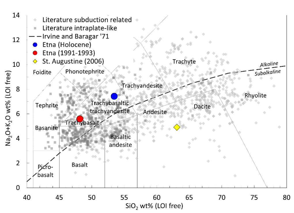
Figure 1. Total Alkali vs. Silica diagram of the samples.
Electromagnetic measurements and mixing formulas
The electromagnetic measurements were carried out with a two port Vector Network Analyzer (VNA), employing a cage coaxial cell and using the experimental procedure and setup described in [11]. The complex permittivity ε and magnetic permeability µ were estimated by using the Nicholson-Ross-Weir algorithm and the equations slightly modified in [12]:

![]()
where Fg is a factor related to the geometry of the cell, Γ and Ψ are the reflection and transmission coefficients, le = 5 cm is the electrical length of the cell, c is the velocity of the light in a vacuum and ν is the frequency. The complex effective permittivity of the two phases granular rock-air was studied using Lichtenecker and Bruggeman mixing formulas:
![]()
![]()
where εi and εeare respectively the permittivity of the environment (the solid grains) and inclusions (air) and f = 1- Φ is the volume fraction of the grainsin the sample, with Φ the porosity.
Results and conclusions
Measurements with the VNA were performed on the granular samples at room temperature, for percentage porosities ranging from 31% to 55%. The magnetic permeability µ is not reported because the three samples do not show a magnetic behavior (and then we can consider µ ≃ 1). Fig. 2 illustrates the complex dielectric permittivity as a function of frequency and at Φ = 0.36. Gray areas in the plots show values that are not reliable since at high frequencies the NRW algorithm diverges because of the cell resonances. Data have larger uncertainties at low frequencies due to VNA instrumental limits. The two Etna samples show a similar dielectric behavior, instead the St. Augustine sample has lower values of both real and imaginary part of permittivity. In the end, we fitted at 80 MHz the complex permittivity as a function of porosity using eqs. 3 and 4. In Tab. 1 we show the measurements at Φ = 0.36 and the values obtained with the mixing formulas at Φ = 0. The St. Augustine sample has the lower values of the solid complex permittivity, probably due to its lower iron abundances and higher abundances of SiO2, while the two Etna samples show a similar dielectric behavior. Further measurements will be required in the future in order to identify the relation between the electromagnetic properties and the geochemical compositions of volcanic rocks that can be accounted as good simulants of the surface and subsurface of terrestrial planets, such as Mars and Venus.
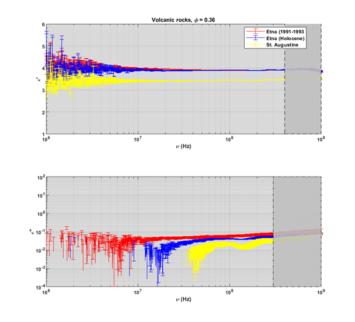
Figure 2. Complex permittivity frequency spectra of the samples.
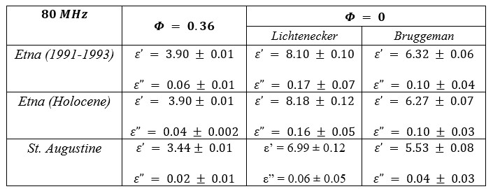
Table 2. Complex permittivity measured at Φ = 0.36 and fitted at Φ = 0 with eqs. 3 and 4.
References
- Orosei R. et al. (2018) Science, 361(6401), 490-493
- Lauro S. E. et al. (2020) Nat. Astron., 5(1), 63-70
- Smith I. B. et al. (2021) Geophys. Res. Lett. 48, 15
- Grima C. et al. (2022) Geophys. Res. Lett. 49.2, e2021GL096518.
- Mattei, E. et al. (2022). Earth and Plan. Sci. Lett. 579, 117370.
- Rust A. C. (1999) Jour. of Volc. and Geoth. Res. 91.1: 79-96.
- McSween Jr et al (2009) Science, 324.5928: 736-739.
- Larsen J. F. et al. (2010). Rapp. tecn. US Geological Survey.
- Calvari S. et al. (1994) Acta Vulcan., 4: 1-14.
- Vona A. et al. (2017) Chem. Geol., 458: 48-67.
- Brin A. et al. (2021) Icarus 114800.
- Mattei E. et al. (2013). IEEE trans. on instr. and meas., 62(11), 2938–2942.
How to cite: Brin, A., Salari, G., Lauro, S. E., Cosciotti, B., Mattei, E., and Pettinelli, E.: Electromagnetic and geochemical characterization of volcanic rock samples in the framework of radar exploration of terrestrial planets, Europlanet Science Congress 2022, Granada, Spain, 18–23 Sep 2022, EPSC2022-956, https://doi.org/10.5194/epsc2022-956, 2022.
Introduction:
The ESA ExoMars rover mission mainly focuses on the search for potential life-relevant molecules (large, non-volatile organic or biological molecules that suggest current or ancient prebiotic activity) at the Mars surface and near-subsurface. The Mars Organic Molecule Analyzer (MOMA) aboard the Rosalind Franklin rover will be a key analytical tool to provide chemical (molecular) information from solid samples collected by the rover. The characterization of the organic content in the sample is the main purpose of the instrument. The MOMA instrument comprises a gas chromatograph coupled to a mass spectrometer (GC-MS) which offers the unique capability to analyze and identify a wide range of organic molecules, including species of interest for life and prebiotic chemistry. Here we present an evaluation of the performance of the instrument from the analysis of a full set of samples of interest for Mars, using the Engineering Test Unit of the GC and MS instruments.
Method:
The samples delivered to MOMA will be analyzed either by UV laser desorption/ionization ion trap mass spectrometry (LDI-ITMS) or pyrolysis gas chromatography ion trap mass spectrometry (pyr-GC-ITMS). Samples containing organic compounds previously detected by LDI-ITMS and/or pyr-GC-ITMS can undergo further analysis through reaction with chemical derivatization reagents before characterization. These reagents (MTBSTFA, DMF-DMA, or TMAH), stored inside sealed capsules, induce a chemical reaction with the sample (in particular with its organic compounds) enhancing the volatility of complex organic species. Due to the need to prevent organic contamination of the Flight Model (FM) and Spare Model (SM) of MOMA, it was not possible to perform extensive analytical tests on them. For that reason, a series of tests were performed by coupling the GC and the MS Engineering Test Units (ETU) which are very close replica of the FM on board the Exomars rover.
The ETU GC (developed in France by LISA and LATMOS laboratories) was mated to the ETU ion trap mass spectrometer (developed in the USA by Goddard Space Flight Center) in a flight-like configuration (Fig. 1) for the coupling campaign. The MOMA GC ETU includes a tank filled with the carrier gas (helium), four separate analytical modules including columns and thermal conductivity detectors (TCDs) and two thermal injection traps. A homemade oven designed and built at LISA is used to mimic MOMA FM ovens. During the pyrolysis of the sample or after its chemical derivatization with one of the three reagents, the volatile compounds are injected and pre-concentrated in one of the traps. The trap is then flash-heated with a backflush carrier gas flow to release the trapped chemical species as quickly as possible into one of the GC columns. The GC column separates the different molecules. They are then ionized by the electron impact ionization source in the MS chamber and analyzed by the linear ion trap mass spectrometer. During the ETU campaign, the derivatization reagents (MTBSTFA, DMF-DMA, and TMAH) are added inside the oven by a syringe mimicking the release of reagent from the MOMA capsules.
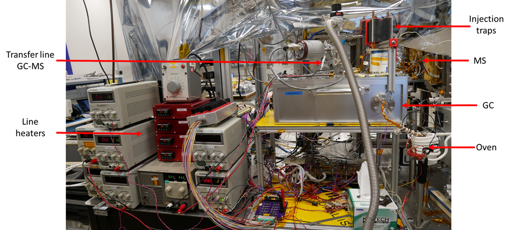
Figure 1: picture of the ETU gas chromatograph and the ETU MS ion trap.
Samples:
Several samples were studied during this campaign. Standard samples (standard gases, amino acids, carboxylic acids) were used to obtain the reference data. Then organic carbon-bearing natural and synthetic (mixing organic molecules and inorganic phases) Mars analog samples were analyzed, using both pyrolysis and derivatization as used in the MOMA instrument. These samples included JSC Mars-1, fragments of Murchison meteorite and synthetic samples composed of an organic-free mineral (vermiculite) doped with phenylalanine, phthalic acid and undecanoic acid. Also a synthetic “unknown” sample was used to run a blind analysis and to test the capability to identify a range of organic species under more realistic analytical conditions. This sample was used to simulate a day in the life of the instrument.
Results and conclusion:
The results described show the current state of end-to-end performance of the gas chromatography-mass spectrometry mode of operation. We show that from a technical point of view, the MOMA instrument works as expected. From a chemical perspective, we have shown that the four different types of MOMA analyses conducted here (pyrolysis and MTBSTFA, DMF-DMA, or TMAH derivatization) are efficient. Specific molecules have been detected (as expected) when using chemical standards. Analysis of the natural and synthetic samples reveals that a large number of molecules are released, and many species have been positively detected and identified (Fig. 2).
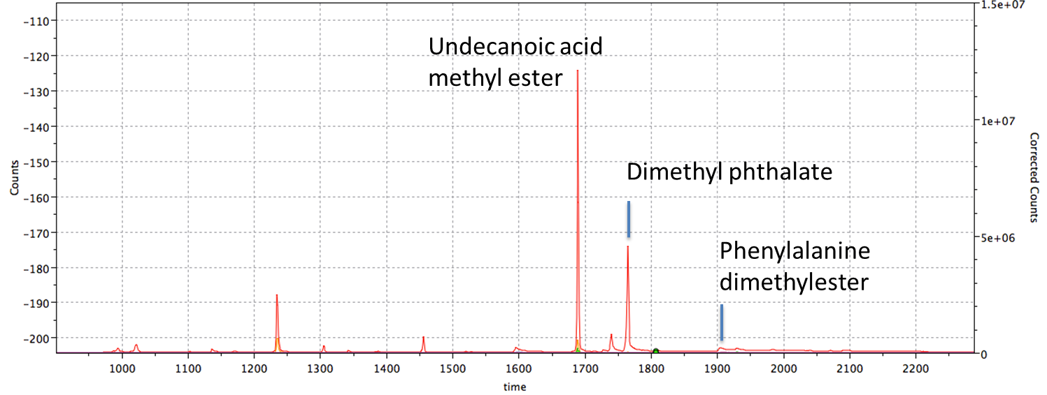
Figure 2 : Total ion chromatogram (TIC) for vermiculite doped with phenylalanine, phthalic acid and undecanoic acid after online DMF-DMA derivatization.
How to cite: Azémard, C., Stalport, F., Kaplan, D., Danell, R., Szopa, C., Buch, A., Chaouche, N., Freissinet, C., van Amerom, F., Grand, N., Zapf, P., Raulin, F., Guzman, M., Fornaro, T., Li, X., Grubisic, A., Siljeström, S., Cottin, H., Brinckerhoff, W. B., and Goesmann, F.: Analytical capabilities of the MOMA GC-MS instrument of the Exomars mission assessed from the analysis of a variety of samples with the Engineering Test Units (ETU), Europlanet Science Congress 2022, Granada, Spain, 18–23 Sep 2022, EPSC2022-1008, https://doi.org/10.5194/epsc2022-1008, 2022.
The Raman Laser Spectrometer (RLS) is part of the analytical payload located inside Rosalind Franklin rover for the Exomars Mission to Mars.
The RLS instrument consists of three main units: 1) the optical head that focus the laser excitation on the sample and collect the scattered light from the same area (with a 50 microns spot); 2) the spectrometer analyzing the Raman signal in the spectral range 150-3800 cm-1 with an average spectral resolution of 8 cm-1 and 3) an electronic control unit in which the laser is included. These units are connected by optical fibers and electrical hardness. The instrument will investigate powdered samples collected by the rover at the surface and subsurface of Mars at the mineral grain scale. (1)
The RLS development stages comprised the development, verification, test and evaluation of the scientific performances of two main models: Engineering Qualification Model (EQM) and Flight Model (FM).
Because the consecutive delays in Exomars launch to Mars an important aspect related with this situation is the evaluation of the scientific performances with time of these models comparing the results obtained at the pre-delivery stage with those obtained at the rover analytical laboratory drawer (ALD) and rover integrated stages.
Additionally it is also of great interest evaluate the scientific results obtained in the framework of dedicated science activities currently ongoing at the ALD and rover levels in which the evaluation of the combined science potential among the three instruments inside Rosalind Franklin rover (MicrOmega, RLS and MOMA) is outstanding.
In the present work interest is devoted to the scientific performances evaluation of the RLS-FM at the different levels: pre-delivery, rover analytical drawer (ALD) and finally integrated on the Rosalind Franklin rover.
For that, observation of the data obtained on the calibration target (CT) is mainly used although data obtained on standard and natural samples at the pre-delivery stage are also presented and discussed.
Instrument response as function of temperature, atmospheric pressure conditions and changes on the main acquisition parameters was evaluated. Estimation of the different band parameters observed (band position, intensity, bandwidth and SNR) allowed performances comparison along the different phases of the process and comparison with the established scientific requirements.
References:
- Rull, S. Maurice, I. Hutchinson, A. Moral et al., Astrobiology, 2017, 17, 627-654.
How to cite: Rull, F., Moral, A., Lopez-Reyes, G., Perez, C., Seoane, L., Zafra, J., Veneranda, M., Manrique, J. A., Rodriguez, E., Rodriguez, P., Belenguer, T., and Prieto, O.: Scientific performances evaluation of the Raman Laser (RLS) FM-instrument for Exomars mission to Mars, Europlanet Science Congress 2022, Granada, Spain, 18–23 Sep 2022, EPSC2022-1068, https://doi.org/10.5194/epsc2022-1068, 2022.
Mars Express has the distinction of being one of the oldest operational spacecraft at Mars, with over 18 years since its injection into Martian orbit in December 2003. Designed for a nominal mission of one Martian year to survey the red planet, it is currently applying for its 9th mission extension. A recent technical review has concluded that Mars Express was technically fit to continue providing excellent science return for the 2023-25 and 2026-28 extension intervals.
The spacecraft subsystems, scientific payload and ground segment are in overall good health, allowing continued smooth mission and science operations. The 3 lifetime-limiting elements of the spacecraft are the gyros, the batteries, and the fuel remaining onboard. The situation of the gyros has been improved by the successful implementation of a gyroless operations mode in May 2018 by the Mars Express teams at ESOC and ESAC. This difficult modification saved the mission and now allows an IMU duty cycle currently reduced to a monthly figure of about 3 to 4 % of the original usage. Mars Express can expect its gyro lifetime to be extended well beyond the 2025 timeframe.
Studies performed in 2019 and 2020 have shown the spacecraft batteries to be much less degraded than had previously been assumed. The findings of these studies were substantiated in subsequent eclipse seasons. A new battery power model now used operationally allows for more flexibility in science planning particularly during eclipse seasons. The longest, most challenging eclipses of the mission were passed successfully in 2021. With shorter eclipse durations in the coming years the outlook is very favourable for continuing to operate the batteries well beyond 2030.
The fuel situation remains satisfactory based on regularly actualised estimates and on a very low fuel consumption (assuming no safe modes; the last one was in 2011). The estimated ~3kg of usable hydrazine (with high confidence based on the Venus Express experience) left onboard can take the spacecraft mission operations to beyond 2030 with the current load of science operations.
Planning and execution of science operations have been improved by upgrades to the mission operations run from the MOC at ESOC and to the Science Ground Segment operations done at ESAC near Madrid. More flexible, rationalised and in some cases even reduced constraints are now in place which enhance the capability of the spacecraft and its payload in performing scientific observations and data taking.
Finally, new science opportunities are presenting themselves in the coming years, illustrated recently by the routine implementation of mutual radio occultations between Mars Express and the ExoMars Trace Gas Orbiter. This will greatly expand the number of atmospheric observations in the future. Automated dual-band radio science occultation observations have now been implemented at egress. The MARSIS subsurface radar is implementing two new promising modes of operation, one to investigate the subsurface at a better sampling rate and one to characterise Phobos, the largest Martian moon and future target for Japan’s MMX mission. Another proposed mission capability will be to perform active sounding of the local plasma environment using combined operation of the ASPERA particle detector and the MARSIS radar. MELACOM relay operations have increasingly taken place with regular Mars Surface Laboratory overflights and were also recently upgraded to implement CNSA’s Zhurong rover overflights and prepare for supporting the ExoMars rover mission as well as other NASA landed assets. These are only a limited set of examples of how Mars Express keeps delivering new and exciting science return.
Interplanetary missions can operate over many years and learning how to use the technology in ways that were maybe not part of the original operational concept is an incredibly important ability. The above demonstrates that the Mars Express teams have been able throughout the mission’s many years of life to render Mars Express a better spacecraft now than at any time before, with in-flight upgrades that kept the mission flying. Those teams were able to make such changes thanks to: robust in-house control and support of the ESAC-run MAPPS planning software allowing for continuous improvement; Flight Control Team with enough skill and resources to modify and fully test the flight code; instrument teams with enough funding and support to allow for software updates/testing late in the mission. This might help younger and upcoming missions assemble the resources now so that they can attempt life-extending changes later.
Combining a special set of payload instruments onboard Mars Express, very resilient spacecraft and payload health and a favourable orbit configuration, this makes for a still unique mission at Mars, very much complementary to newer orbiting elements with different capabilities. ESA is getting the most out of Mars Express and will continue to do so in the coming years, contributing to and enhancing the international cooperation at Mars.
How to cite: Martin, P., Titov, D., Wilson, C., Godfrey, J., Cardesin-Moinelo, A., Blake, R., Dressler, T., Lucas, L., Johnstone, A., Mueller, M., Wood, S., Esquej, P., Merritt, D., Sierra, M., Marin-Yaseli de la Parra, J., Heather, D., Grotheer, E., Breitfellner, M., and Muniz-Solaz, C.: Getting the Most Out of Mars Express, Europlanet Science Congress 2022, Granada, Spain, 18–23 Sep 2022, EPSC2022-1080, https://doi.org/10.5194/epsc2022-1080, 2022.
Mars Express
With almost two decades of Mars observation behind it, Mars Express remains a dependable and highly productive mission.
Recent science highlights include (1) continued mapping of subsurface reflectors beneath the south polar layered ice deposits, and associated work to explain the cause of these reflections; (2) a global map of minerals on Mars with 200 m/px resolution, obtained from analysis of infrared spectra; (3) release of 50 m resolution Digital Elevation Models based on HRSC stereo topography for quadrangles covering an ever-increasing proportion of the global surface; (4) detailed characterization of the landing sites of the ESA, NASA and Chinese rovers; (5) a global climatology of ozone and water from both nadir and occultation observations and its relation to atmospheric dust; (6) transient atmospheric phenomena, such as a recurrent orographic cloud feature at Arsia Mons; (7) detailed investigation of the ionospheric structure, its variability, and coupling to the lower atmosphere; (8) continued monitoring of both the upstream solar wind conditions and of downstream escaping ions; (9) detailed study of Phobos during flybys at altitudes as low as 50 km.
Spacecraft and instrument teams continue to implement new and improved observation modes. One example is new MARSIS instrument software which now allows raw data to be returned from much longer subsurface sounding passes, improving the search for basal reflectors beneath polar ice caps; another example is mutual radio occultation observations between Mars Express and ExoMars Trace Gas Orbiter, potentially providing vertical profiles of ionospheric electron content with good spatial and temporal coverage.
ExoMars Trace Gas Orbiter
TGO has now completed two full Martian years of observations.
Highlights include (1) continuing non-detection of methane, with upper limits as low as 20 ppt by volume. Reconciling this continued non-detection by TGO with the background levels of several hundred ppt in Gale crater by MSL remains an enigma, stimulating further research. (2) detection of HCl, the first reported halogen-containing species in the atmosphere of Mars. (3) further detail of the transport of water to high altitudes, a critical step in the escape of water from Mars. (4) mapping of atomic hydrogen in the top 1-2 m of regolith, indicative of water ice and hydrated minerals, suggesting surprisingly high abundances of subsurface water ice in low latitude regions including one in central Valles Marineris; and (5) continued acquisition of 5 m colour imagery and digital elevation models over a wide range of terrain and target types, including landing site characterization.
Future plans: Mission extension cases for both missions have been submitted for the years 2023-2025 and 2026-2028. The extension of the observations would allow several new and optimized observation types; in particular, it will allow many collaborative observation opportunities with other missions and with ground- and space-based observatories. Of particular note are joint observations with James Webb Space Telescope, for which dedicated observations of Mars are due to be conducted in 2022-2023. Science goals include mapping of the water D/H ratio, search for trace gases including methane, and mapping of thermospheric structure using 4.3 μm CO2 emission; the full-disk views provided by JWST are highly complementary to the vertical profiling and long temporal coverage provided by MEx and TGO.
How to cite: Wilson, C., Titov, D., Martin, P., Cardesin Moinelo, A., Frew, D., Carter, J., Giuranna, M., Holmstrom, M., Montmessin, F., Orosei, R., Paetzold, M., Roatsch, T., Sanchez-Lavega, A., Korablev, O., Mitrofanov, I., Thomas, N., and Vandaele, A. C.: Mars Express and Trace Gas Orbiter – status, science highlights, plans, Europlanet Science Congress 2022, Granada, Spain, 18–23 Sep 2022, EPSC2022-1136, https://doi.org/10.5194/epsc2022-1136, 2022.
TP6 | Martian dust and clouds: from lab to space
Due to the specific atmospheric pressure of a few mbar, Mars is the only planet in the Solar System where thermal creep gas flow occurs naturally within its soil [1,2,3,4,5,6]. As with most flows, this comes with pressure variations. Especially below the top layers of grains, an overpressure develops which sets the soil under tension and supports the lifting of grains from the ground [1,2]. In de Beule et al. 2015, the thickness of an ejected dust layer was measured to be on the order of 200 µm, though upward directed (lifting) forces might also be present further down. This is also in agreement to numerical calculations [2,7]. However, pressure varies on rather small distances of sub-mm which is not easily measurable in a granular bed directly, as small disturbances or changes in the setting already influence the gas flow. So any method of verification of a sub-soil overpressure seems desirable.
Here we use diffusive waves spectroscopy to study the subtle motion of grains within the soil. Illuminating the side of a model soil with a laser beam, scattering and interference lead to a speckle pattern. This pattern changes if particles slightly move. Therefore, a correlation of the patterns over time gives positions depending on the depth where grains move more or less, showing a stratified soil with respect to motion. Among other features, we find a first minimum of particle motion below the surface which shows the characteristic pressure dependence of thermal creep. Specifically, a characteristic maximum depth of about 2 mm is found at about 4 mbar. This depth is somewhat larger than found by de Beule et al. 2015 but in view of the different methods, our measurements are yet another verification that thermal creep sub-soil overpressure is very likely a general mechanism on Mars supporting particle lift [8].
- C. de Beule, G. Wurm, T. Kelling, M. Kuepper, T. Jankowski, and J. Teiser, The Martian Soil as a Planetary Gas Pump, Nature Physics, 10:17-20, 2014.
- C. de Beule, G. Wurm, T. Kelling, M. Köster, and M. Kocifaj, An Insolation Activated Dust Layer on Mars, Icarus, 260:23-28, 2015.
- M. Kuepper and G. Wurm, Thermal Creep Assisted Dust Lifting on Mars: Wind Tunnel Experiments for the Entrainment Threshold Velocity, Journal of Geophysical Research – Planets, 120:1346-1356, 2015.
- M. Kuepper and G. Wurm, Amplification of Dust Loading in Martian Dust Devils by Self-Shadowing, Icarus, 274:249-252, 2016.
- F. Schmidt, F. Andrieu, F. Costard, M. Kocifaj, A.G. Meresescu, Formation of recurring slope lineae on Mars by rarefied gas-triggered granular flows. Nat. Geosci. 10:270–273, 2017.
- M. Koester, T. Kelling, J. Teiser, and G. Wurm, Gas Flow within Martian Soil: Experiments on Granular Knudsen Compressors, Astrophysics and Space Science, 362:171 1-10, 2017.
- M. Kocifaj, J. Klačka, T. Kelling, G. Wurm, Radiative Cooling within Illuminated Layers of Dust on (Pre)-Planetary Surfaces and its Effect on Dust Ejection, Icarus, 211:832-838, 2011.
- T. Bila, J. Kollmer, J. Teiser, and G. Wurm, Thermal Creep on Mars: Visualizing a Soil Layer under Tension, (in prep), 2022.
How to cite: Wurm, G., Bila, T., Teiser, J., and Kollmer, J.: Martian Soil under Tension: Visualizing Thermal Creep Gas Flow by Diffusive Wave Spectroscopy, Europlanet Science Congress 2022, Granada, Spain, 18–23 Sep 2022, EPSC2022-65, https://doi.org/10.5194/epsc2022-65, 2022.
The atmosphere of Mars is driven by different cycles – seasonal cycles of temperature, dust, ice, water vapour, CO2, etc. – which are coupled through transport: dust is blown from the surface by winds, carried aloft where it absorbs solar radiation and heats the atmosphere, impacting temperature, composition and winds. Formation of water ice crystals scavenges dust back from the surface. Water, being involved in the creation processes of clouds, is one of the most important species in the atmosphere. It controls the stability of the atmosphere, dominates its chemistry, and has a radiative impact through the formation of clouds.
Dust is present everywhere on Mars, yet its abundance, physical properties, size distribution as well as impact on the composition, structure and dynamics of the atmosphere has today only barely been addressed and understood. However, knowledge of the characteristics of aerosols (such as dust, ices, clouds and haze) is crucial for the interpretation of the IR and UV spectra because they absorb in these spectral regions, and their absorption signature overlaps the absorption features of other species (such as O3 in the UV), and they regulate the travelling path of light in the atmosphere through absorption and (multiple) scattering. Their impact is difficult to accurately estimate because their spectral characteristics are not known with enough accuracy.
The goal of the ROADMAP project (ROle and impAct of Dust and clouds in the Martian AtmosPhere) is to better characterize the Martian dust and clouds in terms of size, shape and loading within the atmosphere, but also to provide laboratory reference data which will be used to improve our knowledge on the genesis, transport and impact of dust and clouds on the Martian atmosphere.
The team behind the RoadMap project brings together the laboratory community, scientists involved in space missions and numerical modellers to promote synergies through their different perspectives and experiences: laboratory scientists understand the reference data and know-how to extract the most value from their experiments; mission scientists know the intricacies and potential of the instruments and the details of their calibration; numerical modellers know what data, information and parameters are most pertinent to their simulations and how best to interpret the results.
We will describe the methodology behind the project and show how we intend to improve space exploration (observation and modelling of the atmosphere) using new laboratory results (dust resuspension induced by saltation, scattering properties, etc).
The RoadMap (ROle and impAct of Dust and clouds in the Martian AtmosPhere) project has received funding from the European Union’s Horizon 2020 research and innovation programme under grant agreement No 101004052.
How to cite: Vandaele, A. C., Merrison, J., Wurm, G., Munoz, O., Jardiel, T., Lindqvist, H., Wolff, M., Neary, L., Willame, Y., Piccialli, A., Trompet, L., Flimon, Z., Abesha, A., Becker, T., Martikainen, J., Gomez-Martin, J. C., and Peiteado, M.: RoadMap to understand the role of dust in the atmosphere of Mars, Europlanet Science Congress 2022, Granada, Spain, 18–23 Sep 2022, EPSC2022-576, https://doi.org/10.5194/epsc2022-576, 2022.
Thermal infrared observations made from the surface of Mars by the Perseverance rover and from orbit by the Emirates Mars mission enable the retrieval of dust aerosol optical depth at all local times, both day and night. Observations from the rover are useful for characterizing the localized, short timescale changes in dust optical depth, particularly during dust storms, while observations from the orbiter and useful for identifying global trends and temporal variations on longer timescales, from diurnal to seasonal. Together, these two vantage points provide complementary information that helps to understand the variations of dust over different temporal and spatial scales.
1. Introduction
1.1 Perseverance TIRS data:
The Thermal InfraRed Sensor (TIRS) package on the Perseverance rover consists of five sensors used to characterize the upward and downward fluxes of visible and infrared radiation at the rover site (Rodriguez-Manfredi et al., 2021). Of interest here are the sensors TIRS IR1, which covers a broad portion of the thermal-infrared spectrum over the range 6–35 µm and TIRS IR2, which covers the CO2 band between 14.5 and 15.5 µm. Both sensors view upward at an elevation angle centered at 35° above the rover deck. As part of the MEDA suite of atmospheric sensors, TIRS observations are taken systematically throughout the sol at a frequency of 1 Hz. Observations in one-hour blocks are generally taken so that odd-numbered hours are covered on odd-numbered sols, while even-numbered hours are covered on even-numbered sols. In that way the entire 24-hour diurnal cycle is fully covered over a span of 2 sols. These observations are a part of the background baseline set for MEDA that runs essentially every day providing excellent diurnal and seasonal coverage.
We use a radiative transfer model to compute the expected TIRS IR1 and IR2 signal for a given aerosol optical depth and temperature profile. We can then perform the retrieval by varying the atmospheric temperatures and aerosol optical depth to match the values observed by TIRS. The radiative transfer model includes aerosol scattering using a 2-stream approximation (e.g., Smith et al., 2006) and treats absorption by CO2 gas using the correlated-k approximation (Lacis & Oinas, 1991).
1.2 Emirates Mars Mission EMIRS data:
EMIRS is a thermal infrared spectrometer that observes Mars at wavelengths between ~100 and 1600 cm-1 (~100 and 6 µm) at a spectral resolution of 5 or 10 cm-1 (Edwards et al., 2021). From its 55-hour period orbit that varies between 20,000 and 43,000 km altitude, EMIRS raster scans the disk of Mars ~20 times during each orbit to provide a global, synoptic view of Mars that samples all local times, both day and night (Amiri et al., 2021). Over the course of approximately 4 orbits (or 10 days), sufficient observations are taken to provide a broad sampling of all local times at nearly all latitudes and longitudes. The typical footprint size is ~100–300 km, which is consistent with modern global circulation models and is sufficient to provide a detailed global view of the current climate state.
We follow the constrained linear inversion algorithm of Conrath et al. (2000) and Smith et al. (2006) to retrieve atmospheric state parameters that best match the observed spectra of Mars from EMIRS. The radiative transfer model includes a discrete ordinates treatment of multiple scattering (e.g., Goody & Yung, 1989; Thomas & Stamnes, 1999) to accurately model dust and water ice cloud aerosols, and it accounts for the absorptions from CO2 and water vapor gases using the HITRAN database (Gordon et al., 2022) and the correlated-k approximation (Lacis & Oinas, 1991).
Given that the spectral signatures of gases and aerosols are relatively well separated in the spectral range observed by EMIRS, the retrieval is performed sequentially for the atmospheric temperature profile, the column optical depths of dust and water ice aerosol, and the column abundance of water vapor. This sequence can be iterated to obtain a self-consistent solution.
2. Results
Figure 1 shows an example of Perseverance/TIRS retrieval of the complex time history of dust optical depth during a regional dust storm that occurred during January 2022. Here, the sol numbers label midnight LTST. During the active period of this dust event between sols 313 and 317 (5–9 January 2022, Ls=153°–156°) there were numerous spikes in aerosol optical depth with several exceeding unity (at 9 µm). These spikes in aerosol (dust) optical depth occurred preferentially during the day but appear equally in both the morning and the afternoon. Retrievals of dust optical depth outside the dust storm period showed a combination of variations on many timescales from very short (minutes), to diurnal, to the overall seasonal trend.
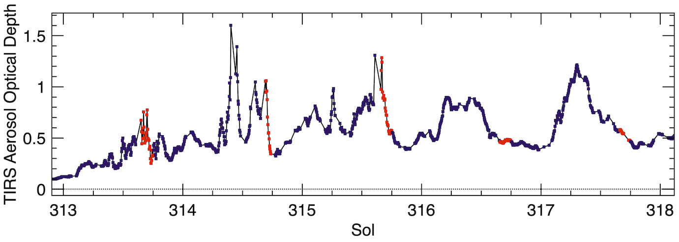
Figure 1. The detailed time history of dust optical depth retrieved from Perseverance TIRS observations during the January 2022 regional dust storm. Local variations on short timescales are apparent.
The January 2022 regional dust storm was also observed by the Emirates Mars Mission/EMIRS instrument. Figure 2 shows a global-scale view of the initiation, growth, and decay of the storm as observed from orbit. Over the course of several days localized dust activity intensified and spread equatorward becoming a regional storm. New dust lifting quickly diminished and the dust was carried by the general circulation to all longitudes before slowly settling out of the atmosphere. These dust retrievals provide global context to those from the rover.
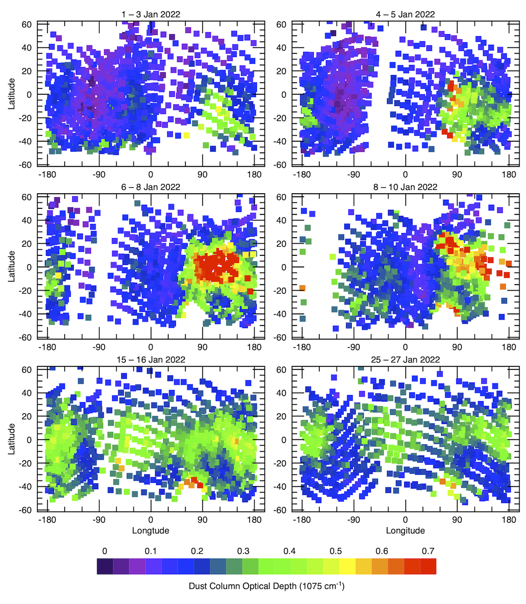
Figure 2. The time history of the global aerosol dust optical depth retrieved from EMIRS observations during the January 2022 regional dust storm. A global view of the evolution of dust is possible from orbit.
References
Amiri, H.E. S. et al., 2021. Space Sci. Reviews, 218:4, doi:10.1007/s11214-021-00868-x.
Conrath, B.J. et al, 2000. J. Geophys. Res., 105, E4, 9509–9519.
Edwards, C.S. et al., 2021. Space Sci. Reviews, 217:77, doi:10.1007/s11214-021-00848-1.
Goody, R.M. & Yung, Y.L., 1989. Atmospheric Radiation: Theoretical Basis. Oxford Univ. Press.
Gordon, I.E., et al., 2022. JQSRT, 277, doi:10.1016/j.jqsrt.2021.107949.
Lacis, A.A. & Oinas, V., 1991. J. Geophys. Res., 96, 9027–9063.
Rodriguez-Manfredi, J.A. et al., 2021. Space Sci. Reviews, 217:48, doi:10.1007/s11214-021-00816-9.
Smith, M.D., et al., 2006. J. Geophys. Res., 111, E12S13, doi:10.1029/2006JE002770.
Thomas, G.E. & Stamnes, K., 1999. Radiative Transfer in the Atmosphere and Ocean, Cambridge Univ. Press.
How to cite: Smith, M., Badri, K., Atwood, S., Martínez, G., Sebastián, E., Apéstigue, V., Arruego, I., Toledo, D., Viúdez, D., Manfredi, J. A., Edwards, C., Smith, N., Wolfe, C., Wolff, M., Christensen, P., Anwar, S., Lemmon, M., AlTunaiji, E., and de la Torre, M.: The diurnal and seasonal variation of dust observed by the Perseverance rover and Emirates Mars Mission, Europlanet Science Congress 2022, Granada, Spain, 18–23 Sep 2022, EPSC2022-599, https://doi.org/10.5194/epsc2022-599, 2022.
Abstract
We present our progress on improvements to the GEM-Mars GCM in the context of the Horizon 2020 RoadMap Project. Through an integrated approach involving lab measurements, micro-modelling, global climate modelling and remote sensing observations, the project aims to better understand the role and impact of dust and clouds on the Martian atmosphere.
Within this project, we use the data from lab experiments and micro-modelling to improve the GEM-Mars Global Climate Model (GCM), with a focus on dust optical properties, mechanisms for dust lifting and microphysical processes.
Introduction
There are still many unknowns and limitations in GCM simulations which cause inaccuracies in the modelled fields, and many of the uncertainties are related to aerosols in the Mars atmosphere. For example, the size distribution and radiative properties of dust and water ice particles are not well known. Through better characterisation of dust from laboratory measurements, we can improve the GCM simulations, and therefore improve the a priori required for data retrieval. As dust is the condensation nuclei for water ice clouds, we can also improve the microphysical representation of these clouds in the model, which in turn will provide more realistic temperatures and global circulation. The interactions in the RoadMap project will also allow to improve the representation of dust lifting, and better define the locations where dust is lifted from the surface, and when.
The GEM-Mars GCM
GEM-Mars is a three-dimensional grid-point based global climate model for the atmosphere of Mars. The physical processes and atmospheric chemistry included are described in Daerden et al., (2019) and Neary and Daerden (2018). GEM-Mars has been applied and evaluated to several recent science investigations including Smith et al. (2021), Bouche et al. (2021), Aoki et al. (2019), Aoki et al. (2022) and Trompet et al. (2022). The impacts of the 2018 global dust storm on the Martian atmosphere were explored in Neary et al. (2019), Daerden et al. (2022a,b) and Khayat et al. (2021). GEM-Mars also participated in a joint modelling exercise for the meteorological conditions at the landing site of the Mars 2020 mission (Newman et al., 2021).
Dust lifting and aerosol properties
Lab experiments using Martian analogue soils were performed by our partners at Aarhus University and the University of Duisburg-Essen and have contributed to an updated formulation of threshold wind stress to describe when lifting may occur. With the same analogue soils (prepared at the Insituto de Ceramica y Vidrio, CSIC-ICV), the scattering properties are being investigated by our partners at the Instituto de Astrofisica de Andalucia (CSIC-IAA). Results from both these lab experiments are then applied and tested in the GEM-Mars GCM.
Microphysics
Currently, GEM-Mars applies a simple dust and cloud scheme. Dust is lifted from the surface in 3 size bins (0.1, 1.5 and 10 µm) and transported by advection, mixing and sedimentation across the atmosphere. Water ice is formed at saturation (100% RH) and condensed into a single Ice Water Content (IWC) tracer. Sedimentation and radiative effects of water ice are calculated by prescribing a fixed particle radius, and assuming the particles are spherical. To obtain a reasonable water cycle over the planet and over the Martian year, the water ice sizes have to vary over altitude. In the current GEM version, these are: 1 μm above 10 km, 2 μm between 5 and 10 km, and 8 μm below 10 km. In addition, to prevent the formation of optically thick clouds over the north polar water ice cap, particle sizes are set to 150 µm below 10 km in summer (Ls = 80°–150°) (Daerden et al., 2022a).
As part of the RoadMap project, we implement a more sophisticated microphysical representation of the formation of ice clouds based on the work of Daerden et al. (2010). The scheme includes the nucleation of water ice on dust particles, deposition and sublimation of water vapour on size-resolved ice and the sedimentation of particles. In Daerden et al. (2010), a one-dimensional model with 100 particle size bins was used. Sensitivity tests using this model helped to improve the computational time for implementation in the 3D GCM. By using fewer particle size bins, we can maintain the basic features of cloud formation while greatly reducing the computational time.
Summary
We will present our progress on the implementation of new dust lifting parameters, and on the development of the size-resolved microphysical representation of dust and clouds. We will first focus on the radiative impact of the increased number of dust particle sizes on the overall global dust cycle.
Acknowledgements
This project has received funding from the European Union’s Horizon 2020 research and innovation programme under grant agreement No 101004052. The authors acknowledge funding by the Belgian Science Policy Office (BELSPO), with the financial and contractual coordination by the ESA Prodex Office (PEA 4000103401, 4000121493).
How to cite: Neary, L. and Daerden, F. and the The RoadMap Team: Improvements to dust and aerosols in GEM-Mars GCM simulations: Results from the RoadMap project, Europlanet Science Congress 2022, Granada, Spain, 18–23 Sep 2022, EPSC2022-637, https://doi.org/10.5194/epsc2022-637, 2022.
1. Introduction
Thermal infrared datasets from planetary bodies have the potential to provide key insights for the understanding of a planet's climate evolution and history: valuable information about composition, temperature and state of the atmosphere can be retrieved from thermal spectral data.
In this work, we present the application of a methodology based on Principal Component Analysis (PCA) and Target Transformation (TT) Factor Analysis (FA) techniques to thermal infrared data of the ExoMars2016 Trace Gas Orbiter (TGO) with the main goal to retrieve the different particulate atmospheric contributions present in the spectra and separate them from the surface contributions.
2. Instrument and dataset
TGO has a suite of spectroscopic instruments for the investigation of the Red Planet in the infrared spectral range known as Atmospheric Chemistry Suite (ACS) [1] consisting of three spectrometers observing Mars in solar occultation, nadir and limb geometry in the Near-InfraRed (NIR), Mid-InfraRed (MIR) and Thermal InfraRed (TIR) spectral channels. Among them, the ACS thermal-infrared channel (TIRVIM) covers the spectral range between 1.7-17 μm with apodized resolution varying from 0.2 to 1.3 cm−1 [1]. TIRVIM has similar capabilities to IRIS (Mariner 9), TES, and PFS in several aspects, but has some advantages: - higher spectral resolution; - better noise equivalent radiance (from 0.08 mW/m2/sr-1/cm-1); - dense spatial coverage (TGO has a circular orbit of 400 km) [1].
Martian TIRVIM spectra acquired along the orbits that cross Elysium Planitia, landing site of the NASA’s Insight (Interior exploration using Seismic Investigations, Geodesy and Heat Transport) lander, were here analyzed. The selected data orbits span from Ls=150°C to Ls=210°C, covering part of the Martian summer and of the Martian autumn going through the autumn equinox in the northern hemisphere of the planet. Corresponding Local Times cover Martian days and nights.
3. Methodology
To analyze the ExoMars TIRVIM data and retrieve and characterize the number of varying atmospheric components present in these data and their spectral shape, a methodology was applied based on a combination of PCA and TT – FA techniques [2, 3]. These techniques are demonstrated to be able to extract the composition of laboratory samples [4, 5]; to extract the principal varying components from a big spectral dataset in the thermal infrared [3], and then to identify them as components of the atmosphere and separate their contribution from surface emission [6]. This methodology, previously successfully adopted for the analysis of TES and PFS data [2, 7], was, here, applied for the first time to the analysis of the new and at higher spectral resolution TIRVIM dataset. Considering that the PCA works best when the different components have significant variation in the data, we selected data where these variations are more likely to occur: the analyzed data cover diurnal as well as seasonal variations.
A list of PFS and TES atmospheric end-members extracted from [3] and [2] were used as initial guess for the TT, to interpret the abstract eigenvectors retrieved from the PCA and attribute them a physically coherent meaning.
4. Results and future developments
Spectral shapes of atmospheric dust and water ice aerosols were recovered from the analyzed TIRVIM data. Comparisons with results previously obtained on PFS and TES data (Figure 1) validate the methodology used and show that it is capable of determining the number of independently variable components and recovering the spectral endmembers present in the TIRVIM data.
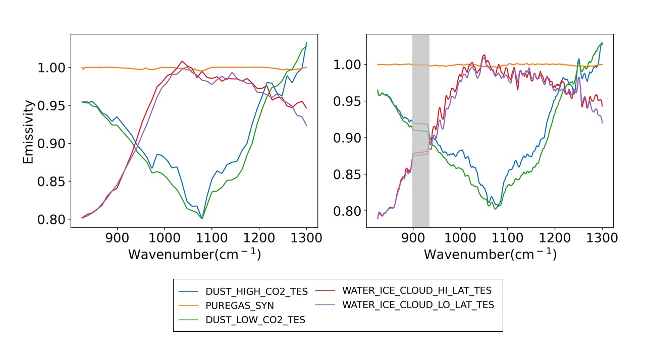
Figure 1. Comparison between the general TES/PFS extracted endmembers [2, 3] (upper panel) and the endmembers extracted from the TIRVIM data in this work (bottom panel). Grey area: wavelength cut due to high instrumental noise.
Deconvolution of the original spectra using the recovered spectral end-members allowed us to obtain the concentration coefficients of the dust and water ice end-members and retrieved abundances maps. The results obtained are promising in terms of identification and separation of the atmospheric components and have strong impact on the identification of surface contributions in the spectra. We are further investigating this point with the main goal of showing the potential of this method to extract valuable information from TIRVIM data not only on the atmosphere, but also on the surface of the Red Planet. Derived surface emissivity products are being analyzed by linear deconvolution analysis with the laboratory spectral database of Martian analogues measured at the Planetary Spectroscopy Laboratory (PSL) of DLR, in Berlin [5].
Acknowledgments
ExoMars is a space mission of ESA and Roscosmos. The ACS experiment is led by IKI, the Space Research Institute in Moscow, assisted by LATMOS in France. The science operations of ACS are funded by Roscosmos and ESA.
References
[1] Korablev et al. (2018) Space Science Review, 214:7. [2] D’Amore M. et al. (2013) Icarus, 226, 1294-1303. [3] Bandfield J.L., Christensen P.R., Smith M.D. (2000) JGR, 105 (E4), 9573-9587. [4] Smith, M.O., Adams, J.B., Johnson, P.E. (1985) JGR, 90, 797-804. [5] Alemanno G., Maturilli A., D’Amore M., Helbert J. (2021) Icarus, 368. [6] Smith M. D., Bandfield J. L. and Christensen P.R. (2000) JGR, 85 (E4), 9589-9607. [7] Maturilli, A., Helbert, J., D’Amore, M. (2009) EPSC2009, Abstract #EPSC2009-106.
How to cite: Alemanno, G., D'Amore, M., Maturilli, A., Helbert, J., Arnold, G., Korablev, O., Ignatiev, N., Grigoriev, A., Shakun, A., and Trokhimovskiy, A.: Particulate atmospheric endmembers retrieval from ExoMars Thermal Infrared (TIRVIM) spectral data, Europlanet Science Congress 2022, Granada, Spain, 18–23 Sep 2022, EPSC2022-862, https://doi.org/10.5194/epsc2022-862, 2022.
The Nadir and Occultation for Mars Discovery (NOMAD) is one of the four instruments on board the 2016 ExoMars Trace Gas Orbiter. The instrument is a suite of three spectrometers, mainly designed to study minor atmospheric species at high spectral resolution (A.C. Vandaele et al., 2015; E. Neefs et al., 2015). Nevertheless, Oliva et al. (2022) demonstrated the capability of NOMAD infrared nadir channel to investigate surface ice composition in the 2.3 – 2.6 μm wavelength range. Ice signatures have been also observed at mid/equatorial latitudes suggesting, after analysis, the first detection of CO2 ice clouds through the study of the narrow 2.35 μm absorption band.
In this work, we also use observations of the NOMAD infrared LNO channel in order to evaluate its capability to detect H2O ice clouds. We present a technique taking advantage of the 2.7 µm strong ice absorption band. For this study, we select LNO spectral orders 167, 168, 169 and combine them to derive a spectral index for H2O ice detection, namely the Frost and Clouds Index (FCI). The acquisition of data during Mars Year 34 and 35 (March 2018 to February 2021) allows us to construct seasonal maps for H2O ice clouds. The results appear in agreement with previous studies focused on Mars Express SPICAM/UV and OMEGA data analysis (Willame et al., 2017; Olsen et al., 2021). FCI is sensitive to the Polar Hood clouds, although the full structure is not detected. Moreover, detections in the Aphelion Cloud Belt (ACB) are limited. This is consistent with previous OMEGA spectrometer observations (Olsen et al, 2021) showing different physical properties between the two main Martian atmospheric structures and making the ACB less detectable in the infrared. We hence derive the LNO channel sensitivity limit for these clouds detection.
Acknowledgements
ExoMars is a space mission of the European Space Agency (ESA) and Roscosmos. The NOMAD experiment is led by the Royal Belgian Institute for Space Aeronomy (IASB-BIRA), assisted by Co-PI teams from Spain (IAA-CSIC), Italy (INAF-IAPS), and the United Kingdom (The Open University). This project acknowledges funding by the Belgian Science Policy Office (BELSPO), with the financial and contractual coordination by the ESA Prodex Office (PEA 4000103401, 4000121493), by Spanish Ministry of Science and Innovation (MCIU) and by European funds under grants PGC2018-101836-BI00 and ESP2017-87143-R (MINECO/FEDER), as well as by UK Space Agency through grants ST/V002295/1, ST/V005332/1 and ST/S00145X/1 and Italian Space Agency through grant 2018-2-HH.0. This work was supported by the Belgian Fonds de la Recherche Scientifique – FNRS under grant number 30442502 (ET_HOME). The IAA/CSIC team acknowledges financial support from the State Agency for Research of the Spanish MCIU through the ‘Center of Excellence Severo Ochoa’ award for the Instituto de Astrofísica de Andalucía (SEV-2017-0709). US investigators were supported by the National Aeronautics and Space Administration. Canadian investigators were supported by the Canadian Space Agency. SR thanks BELSPO for the FED-tWIN funding (Prf-2019-077 - RT-MOLEXO).
References
A.C. Vandaele, et al., 2015. Optical and radiometric models of the NOMAD instrument part I: the UVIS channel. Optics Express, 23(23):30028–30042.
Neefs, et al., 2015. NOMAD spectrometer on the ExoMars trace gas orbiter mission: part 1—design, manufacturing and testing of the infrared channels. Applied optics, 54(28):8494–8520.
Oliva, F., et al., 2022. Martian CO2 Ice Observation at High Spectral Resolution With ExoMars/TGO NOMAD. Journal of Geophysical Research: Planets, 127, e2021JE007083.
Willame, Y., et al., 2017. Retrieving cloud, dust and ozone abundances in the martian atmosphere using spicam/uv nadir spectra.Planetary and SpaceScience, 142:9–25.
K.S. Olsen, et al., 2021 Retrieval of the water ice column and physical properties of water-ice clouds in the martian atmosphere using the OMEGA imaging spectrometer, Icarus, Volume 353, 2021, 113229, ISSN 0019-1035.
How to cite: Ruiz Lozano, L., Karatekin, Ö., Dehant, V., Bellucci, G., Oliva, F., D'Aversa, E., Altieri, F., Carrozzo, F. G., Willame, Y., Thomas, I., Daerden, F., Ristic, B., Patel, M., López Moreno, J. J., and Vandaele, A. C.: Evaluation of the capability of ExoMars-TGO NOMAD infrared nadir channel for water ice clouds detection on Mars, Europlanet Science Congress 2022, Granada, Spain, 18–23 Sep 2022, EPSC2022-946, https://doi.org/10.5194/epsc2022-946, 2022.
TP7 | Atmospheres and Exospheres of Terrestrial Bodies
It is evident that a variety of metals are deposited in the Earth’s mesosphere and lower thermosphere (MLT, ~70-120 km) through meteoric ablation when the cosmic dust particles enter the atmosphere at high entry velocity (11-72 km/s). However, it is still unclear how much and accuarate cosmic dust enters the atmosphere of Mars (though the estimation of global dust input would be a few tons per sol) and what is the difference comparing to Earth’s atmosphere (which has a 1-2 order global input range from different estimations).
We have developed global atmospheric meteoric models of Na, Fe, K, Mg, Ni, Ca, Al, Si, P, S etc) into the Whole Atmosphere Community Climate Model (WACCM) and its vertical extensions to 600 km (WACCM-X) from US National Center for Atmospheric Research (NCAR, termed WACCM-metals), which simulate well the metal layers compared with the available lidar/rocket/satellite measurements.
New observations of some metals for the Martian atmosphere (i.e., Mg+ observations from IUVS (Imaging UV Spectrometer) and Mg+, Na+ and Fe+ from NGIMS (Neutral Gas Ion Mass Spectrometer)) instruments on NASA’s Mars Atmosphere and Volatile Evolution Mission (MAVEN) spacecraft are available from 2014. Therefore, we have incorporated the chemistry of three metals (Mg, Na and Fe) in the Laboratoire de Météorologie Dynamique (LMD) Mars global circulation model (termed as LMD-Mars-Metals), following similar work we have done for the Earth’s atmosphere. The model has been developed by combining three components: the state-of-the-art LMD-Mars model covering the whole atmosphere from the surface to the upper thermosphere (up to ~ 2 x10⁻⁸ Pa or 240 km), a description of the neutral and ion-molecule chemistry of Mg, Fe and Na in the Martian atmosphere (where the high CO2 abundance produces a rather different chemistry from the terrestrial atmosphere), and a treatment of injection of the metals into the atmosphere from the ablation of cosmic dust particles. The LMD-Mars model contains a detailed treatment of atmospheric physics, dynamics and chemistry from the lower atmosphere to the ionosphere. The model also includes molecular diffusion and considers the chemistry of the C, O, H and N families and major photochemical ion species in the upper atmosphere, as well as improved treatments of the day-to-day variability of the UV solar flux and 15 mm CO2 cooling under non-local thermodynamic equilibrium conditions.
We have incorporated the chemistries of Mg, Fe and Na into LMD-Mars because these metals have different chemistries which control the characteristic features of their ionized and neutral layers in the Martian atmosphere. The Mg chemistry adds 7 neutral and 8 ionized Mg-containing species, connected by 42 neutral and ion-molecule reactions. The corresponding Fe chemistry has 39 reactions with 14 Fe-containing species. Na chemistry adds 7 neutral and only 2 ionized Na-containing species, with 32 reactions. The injection rate of these metals as a function of latitude, solar longitude at different pressure levels is pre-calculated from the Leeds Chemical Ablation Model (CABMOD) combined with an astronomical model which predicts the dust from Jupiter Family and Long Period comets, as well as the asteroid belt, in the inner solar system. The model has been evaluated against by Mg+, Na+ and Fe+ observations from IUVS and NGIMS measurements.
The comparison of these metal layers between Earth’s and Mar’s atmospheres will be discussed, which allows us to understand the meteor astronomy, chemistry and transport processes that control the different metal layers in the upper atmosphere on different planets.
How to cite: Feng, W., Plane, J., González-Galindo, F., Marsh, D., Chipperfield, M., Carrillo-Sánchez, J. D., Janches, D., Chaufray, J.-Y., Forget, F., Millour, E., Crismani, M., Tyo, R., Schneider, N., and Benna, M.: Differential Ablation of meteoric metals in the LMD-Mars-Metals and NCAR WACCM-Metals models, Europlanet Science Congress 2022, Granada, Spain, 18–23 Sep 2022, EPSC2022-236, https://doi.org/10.5194/epsc2022-236, 2022.
The study of the atmospheric circulation in the planets and moons of our solar system and exoplanets is critical for the advances in Meteorology. In slowly rotators like Venus, Titan and tidally-locked exoplanets, the Coriolis effect is too weak to balance the pressure gradients and other metric terms (centrifugal forces) generate a different balance called “cyclostrophic”. For reasons yet not fully understood, these slowly rotating bodies tend to exhibit atmospheres which rotate much faster than the solid globe, a phenomenon called atmospheric “superrotation”. Venus constitutes the most extreme case known in our solar system, with its clouds rotating up to 60 times faster than the surface, although numerical models yet fail to accurately reproduce this superrotation, especially at the deeper atmosphere. Besides, despite the richness of information provided by the space missions that explored Venus in the past and the varied and numerous Earth-based observations, accuracy in wind measurements at present is yet insufficient to isolate and characterize the several contributors of the observed speeds of the lower clouds of Venus located within 48-60 km. As a result, the net meridional circulation, influence of the solar tides or the magnitude of transient waves and eddied are yet uncertain.
In this work we intend to provide new insights about the circulation at the deeper atmosphere of Venus obtaining wind speeds with an accuracy better than 1 m·s-1 taking advantage of the long-term coherence of the lower clouds’ patterns, which enables confidently tracking cloud tracers in images separated by more than 5 hours. These high-precision winds were obtained from sequences of images taken at 1.74, 2.26 and 2.32 µm by space missions Venus Express/VIRTIS-M (2006-2008) and Akatsuki/IR2 (2016), as well as with pairs of images acquired co-ordinately by Earth-based telescopes located at different geographical locations: IRTF/SpeX in Hawaii and HCT/IRCAM in India (May and July 2004, December 2010), IRTF/SpeX in Hawaii and NOT/NOTCam (July 2020). Our results extend those from VIRTIS-M recently published by Gorinov et al. (Atmosphere 2021, 12, 186) and confirm some of their results.
How to cite: Peralta, J., Galeote, A., Lee, Y. J., Bullock, M., Young, E., Machado, P., Espadinha, D., and Baena, R.: The circulation at the nightside lower clouds of Venus with high-precision winds, Europlanet Science Congress 2022, Granada, Spain, 18–23 Sep 2022, EPSC2022-398, https://doi.org/10.5194/epsc2022-398, 2022.
TP11 | Structural Geology and Deformational Histories of Terrestrial Bodies
Introduction: In the Martian North Polar Cap, troughs are formed and enlarged by the erosive action of katabatic winds, blowing perpendicularly with respect to steep edges of the cap. Along these valleys deeper layering of the polar deposits are often exposed making it possible to study the stratigraphy of the upper part of the polar cap [1]. We focused our attention on a 140 km long and 500 m high scarp located in the North-Western edge, facing Olympia Planum, and where part of the North Polar Layered Deposits (NPLD) are exposed. NPLD deposits are finely layered and laterally continuous sequence of light and dark strata with sporadic unconformities in between, whose periodicity has been attributed to climatic and orbital variations [2]. In the polar cap, Tanaka et al. [3] has distinguished different polar units by means of surface image interpretation, hence our scarp exposes Planum Boreum 1 unit overlapped by Planum Boreum 3 unit, both composed of variable ice/dust content, but different thickness. Putzig et al. [4] identified instead seven units inside the polar cap on the basis of the pattern of radar reflections in the radargram-based stratigraphy thanks to the data provided by SHARAD. The stratigraphic sequence of our interest correlates with the upper part of the packet-inter-packet sequence of the unit G by Putzig et al. [4]. The aim of our work is to relate the composition and stratigraphy of the visible layered deposits with the subsurface radar reflectors, using the data acquired by the NASA Mars Reconnaissance Orbiter instruments.
Data selection: We performed stratigraphic and geomorphologic interpretation on images of the Context Camera (CTX) and High Resolution Imaging Science Experiment (HiRISE); band ratios and spectral signatures on a hyperspectral cube of the Compact Reconnaissance Imaging Spectrometer for Mars (CRISM); subsurface reconstructions on radar reflectors obtained by the Shallow Radar (SHARAD). The integration of the results obtained by such a multi-score data-set underlies the possibility to join the SHARAD stratigraphy with the stratigraphic record recognisable at the surface including its compositional variability (Fig.1).
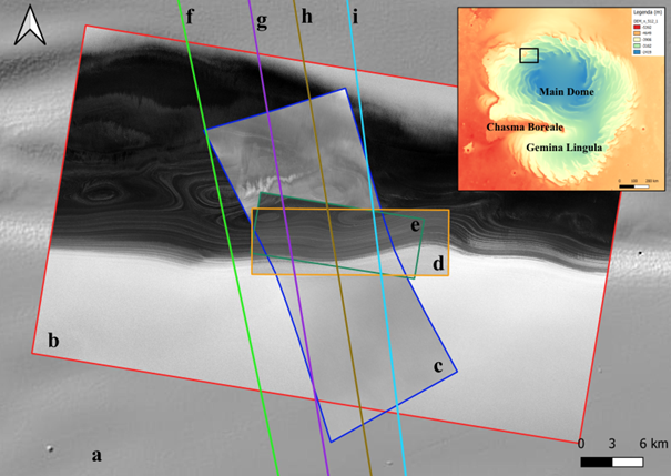
Fig.1 – Data-set: MOLA DEM (a), CTX image (b), CRISM cube (c), HiRISE images (d, e) and SHARAD radargram tracks (f, g, h, i). Black rectangle in the North Polar Cap region shows the study area.
Spectral analysis: Spectra for five Regions of Interest (ROIs) of about 50 pixels were acquired and are shown in Fig.2a-b.
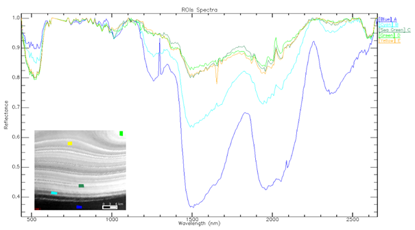
Fig.2 – (a) Regions of Interest over CRISM image detail; (b) Plot of five ROI average spectra: each colour line represents a ROI spectrum (continuum is removed).
The exposed stratigraphy is composed of different amount of dry ice, water ice and basaltic dust [3]. Spectra A and B are well distinguishable, whereas the signatures of C, D and E appear similar, indicating comparable compositions. Spectrum A exhibits well developed water-ice absorption bands (1.5 and 1.95 µm), less development of same peaks might imply an increase of dry ice content. The 1 µm peak (water ice) is well visible in both A and B spectra, but less evident in C, D and E. Multiple absorptions at 1.65 and 2.06 µm, associated to CO2, are well visible in C, D and E. Other absorption bands (at 0.50, 1.02 and 2.30 µm for example) can be related to femic and aqueous alteration minerals. Spectrum A is similar to the signature of pure water ice, with less altered minerals, while C, D and E appear to be characterized by dry ice and femic minerals. Spectrum B appear to be transitional between these two end-members.
Spectral indexes: Spectral indexes were produced using CRISM Analysis Toolkit (CAT) [5]. Indexes allowed us to create false colour images to highlight the presence/absence of specific minerals. Example of these are shown in Fig. 3 (see FED for the index definition).
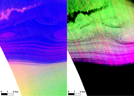
Fig.3 – Two false colour images created with spectral indexes (a) BDI1000VIS_BD15002_BD1435 representing ice compositions and (b) OLINDEX3_LCPINEX2_RBR to highlight mineral composition.
Mapping and correlation to radar reflectors: Geological units were identified on CRISM and CTX data on the basis of morphology, composition, albedo and their stratigraphic relationship. Fig.4 displays the mapped units.
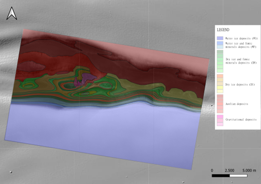
Fig.4 – Geological map and relative units. WI-units: water-ice-rich deposits (blue), WF-unit: water ice and femic minerals deposits (light blue); DF-units: dry ice and femic minerals deposits (green); DI-units: dry-ice-rich deposits (yellow); Aeolian deposits (red); Gravitational deposits (purple).
Fig.5 shows the geological units correlated with radargrams features. Variations of dielectric constant among strata are due firstly to presence of water ice in the surficial layers and dry ice in deeper ones, secondly to different amount of dust in radar units. These affect the signal reflectance: stronger if it is from water-ice layers. Additionally, high content of dust significantly decrease the radar signal, so units appear darker [4] [6]. The lines in Fig.5 represent lower contact of the geological units.
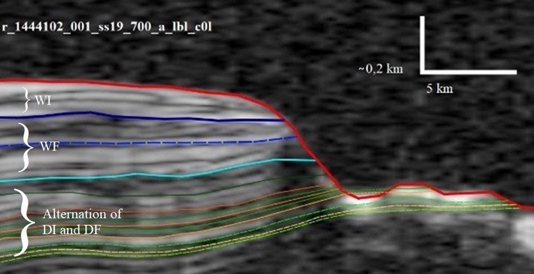
Fig.5 – Correlation between geological units and radar reflectors. The colours of units are the same of geological map (vertical axis in time). Section track is shown in Fig.1.
Discussion and conclusions: We provide a detailed compositional and geometrical characterization (using CRISM, HiRISE, CTX) of outcropping layered deposits of the North Polar Cap, to evaluate the potential for performing sound stratigraphic correlations with the subsurface reflectors identified in SHARAD radargrams. At a scale of single layers, compositional variations of basaltic dust content in the stratigraphic sequence were identified. This variability is visible especially in dry-ice-rich layers. Basaltic dust showed aqueous alteration, especially in water-ice-rich strata.
Acknowledgments: We acknowledge support from the EU’s H2020 research and innovation program under grant agreement N° 871149 (GMAP).
References: [1] Masse, M. et al. (2012) Earth and Planetary Science Letters, 317, doi: 10.1016/j.epsl.2011.11.035; [2] Byrne, S. (2009) Annual Review of Earth and Planetary Science, 37, doi: 10.1146/annurev.earth.031208.100101; [3] Tanaka, K. et al. (2008) Icarus, 196(2), doi: 10.1016/j.icarus.2008.01.021; [4] Putzig, N. et al. (2009), Icarus, 204(2), doi: 10.1016/j.icarus.2009.07.034; [5] Viviano-Beck, C. et al (2014), Journal of Geophysical Research, 119(6), doi: 10.1002/2014JE004627; [6] Lauro, S. et al. (2012), Icarus, 219(1), doi: 10.1016/j.icarus.2012.03.011.
How to cite: Costa, N., Massironi, M., Penasa, L., Nava, J., Pozzobon, R., and Ferrari, S.: Compositional and subsurface analysis of an outcrop close to Olympia Planum on Mars, Europlanet Science Congress 2022, Granada, Spain, 18–23 Sep 2022, EPSC2022-167, https://doi.org/10.5194/epsc2022-167, 2022.
The ExoMars rover mission will be looking for biosignatures (i.e. signs of past and present life) in Oxia Planum, Mars [1]. The landing site is located between 16° and 19° N and 334° to 337° E where the ancient cratered terrains transition into the low-lying plains of Chryse Planitia. The area of interest is situated between Ares Vallis and Marwth Vallis in a wide basin at the outlet of Cogoon Vallis. The fractures, extensively spread over the terrains of the landing site, range from meters to decameters in spacing and length and have been preliminary interpreted as desiccation cracks or the result of burial and unloading of sediments [2,3]. We mapped these fractured terrains and we tested an automatic method for alignment tracing which contributes to our study in an effort to evaluate the directional aspects of fracturing and their spatial distribution within the study area.
The data we used come from VNIR pushbroom imager camera HiRISE, which produces the highest resolution images of the martian surface (25 to 60 cm/pixel) [4]. 31 greyscale HiRISE RED products (25 cm/pixels) and three HiRISE colour product (60 cm/pixel) covering the landing ellipse were selected and downloaded from the Planetary Data System (PDS) [5], and imported into QGIS (version 3.24.1 Tisler) [6]. To map these fractures over a submeter resolution basemap within the ≥1000 km2 landing ellipse area, we opted to use a 1:5000 scale. We mapped the boundaries of the fractured area as lines, generating category areas from the boundaries of the mapped area through the Mappy QGIS plugin [7]. We classified the fractures by their association with sand, dunes, TARs and ridges. Using the resulting map of the fractured terrains, we placed a 200 m2 Scan Area on a place where fracturing was more evident: we extracted HiRISE data that was input into the Slope Intersect Discrete Analysis (SID) software version 3.04-10 for automatic tracing of the fractures. The results of automatic tracing, whose algorithm is based on a modified Hugh transform [8], was further processed in to GRASS GIS [9]: the GRASS Toolset v.clean was used to snap vertices of SID output. To compare the manual and automatic methods, the Scan Area input by SID has been used to manually trace fractures at 1:1000 scale, whose orientation in the space was obtained using Daisy software version 3-5.51-3. The map of the fractured terrains was then used to place multiple Scan Areas where fracturing is more evident (Fig.2). The automatic fracture tracing method will be applied on other areas of interest in future studies.
We classified fractured terrains into three categories where we placed 28 Scan Areas (Fig.1) : we placed nine of them in terrains characterized mainly by fractures (MF, lower portion of the map), 10 in terrains associated with the presence of linear topographic rises (ridges) (RF, central portion of the map) and nine in fractured terrains with an abundance of sand and dunes (SF, upper portion of the map). 507 fractures were traced manually ranging 1.14-68.4 m in length (Fig.2, b). In the automatic method, SID mapped 1712 elements between 2 and 21 m in length (Fig.2, a). Regarding the directional Azimuth-Frequency analysis carried out by Daisy, the average orientation is very similar: fractures traced manually indicate a value of 92.26° (sd: 12.5°) and fractures traced via SID correspond to a value of 93.06° (sd: 15.97°) (Fig.2, a, b below).
The spatial distribution of fractures traced manually is homogeneous, including both the longest and the shortest fractures. The few areas where the absence of fractures is observed are those where there is a strong cover of sand. The longer fractures do not create intersections, if not with the shorter ones, which cross each other, forming small networks. The homogeneous distribution of manually traced fractures is the same as those traced unsupervised via SID. The differences instead occur mainly in the number and in the length of lines traced in the two methods: SID’s sensitivity to low variations of DN result in a greater number of identified fractures through segments with a defined minimum and maximum length. However, not all manually traced fractures have been identified by SID. No matter how efficient the GRASS GIS toolset is, fractures traced by SID too far apart from eachother were not considered a single element, which the human interpretation would have done. As far as orientation is concerned, the two methods show very similar values.
This study shows how, although the clear differences between manually and automatic method, the latter may prove to be efficient, even considering their limitations. SID’s fracture tracing in fact guarantees a strong effectiveness for the calculation of their orientations. Further analysis in the Scan Areas placed on the fractured terrains of the landing ellipse will verify whether or not there are anisotropies in the orientation of the fractures, which will help improve our knowledge about the formation and evolution of Oxia Planum.
References
[1] Vago et al.(2017), Astrobiology, Vol. 17, No. 6-7. [2] Quantin-Nataf et al. (2021) Astrobiology 21, 345. [3] Bowen et al. (2022) Planetary and Space Science Volume 2014. [4] McEwen et al. (2007) Journal of Geophysical Research: Planets Volume 112, [5] McMahon (1995) Planetary and Space Science Volume 44 [6] Casagrande et al., (2014) Dario Flaccovio Editore p. 220 [7] Penasa et al. (2020) European Planetary Science Congress, Volume 14 [8] Hough (1959) HEACC, Proceedings of the 2nd International Conference on High-Energy Accelerators and Instrumentation [9] Neteler and Mitasova (2013) The Springer International Series in Engineering and Computer Science
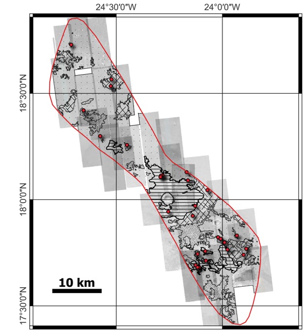

Figure 1 – Fractured terrains mapping and Scan Area locations within the ExoMars landing ellipse. Geospatial data is in simple cylindrical projection, considering Mars Sphere (IAU2018:49910).
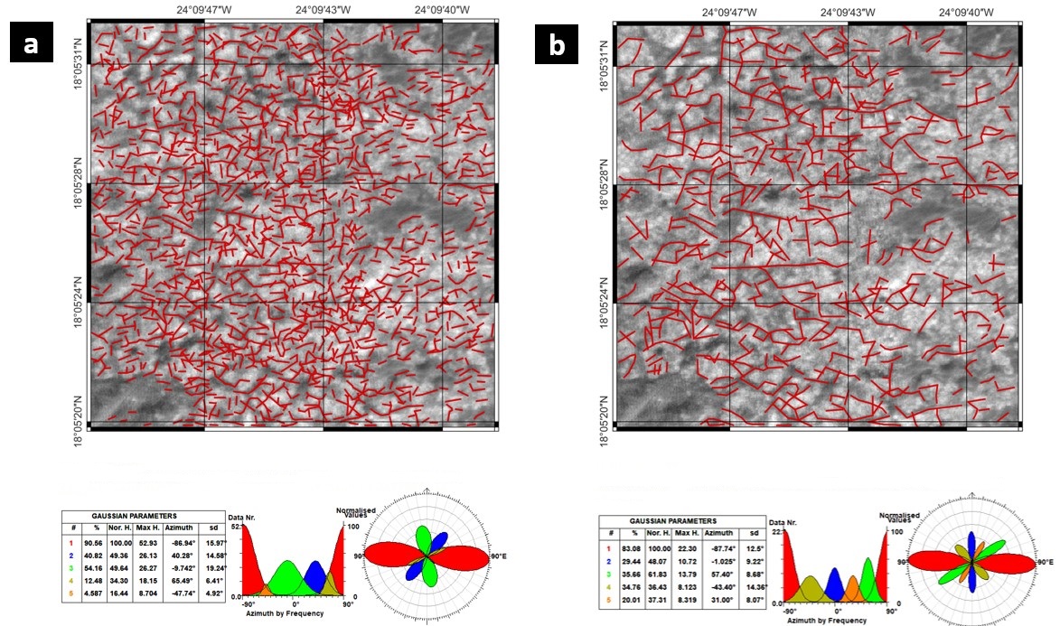
Figure 2 - Comparison between automatic (a) and manual tracing (b). The tables show results of the directional analysis effectuated by Daisy.
How to cite: Apuzzo, A., Frigeri, A., Salvini, F., Brossier, J., De Sanctis, M. C., Costa, N., and Schmidt, G. W.: Automatic Fracture Tracing by Image Processing on Oxia Planum, Mars, Europlanet Science Congress 2022, Granada, Spain, 18–23 Sep 2022, EPSC2022-350, https://doi.org/10.5194/epsc2022-350, 2022.
INTRODUCTION
In recent years, the Martian world has drawn the attention of researchers all over the globe. Mars’ rich geological record and fascinating history led scientists and space organisations to be keen on studying the planet more closely. Several studies on Mars are primarily focused on determining the potential for life. (Nazari-Sharabian et al., 2020). The similarities between Mars and early Earth are a big part of why people want to study it. Little has changed on Mars since the Hesperian epoch, 2.9 billion years ago, due to the lack of plate tectonics (Victoria et al., 2018). As a result, unlike Earth, it is possible to look at Mars as a blank canvas due to no artificial structural advancements. The discovery of geological features that resemble small valleys and river plains (Rice et al., 2008) has only raised the possibilities of finding water on Mars in some form. Many dramatic events occurred on Mars' glacial past, leading to the construction of valleys, river plains, glacial landforms, and other features. We have recently learned a lot more about such features.
Mars’ extreme glacial history led to significant changes and the formation of interesting features such as glacial-like landforms on the planet. Changes in the orbital and rotational parameters have allowed ice from ice-rich polar regions to shift towards the equator (Mischna et al., 2003). This process is termed mid-latitude glaciation (Hepburn et al., 2020; Milliken et al., 2003). Furthermore, these formations have flow-like geomorphology as shown in figure 1, indicating the presence of ice underneath these landforms (Holt et al., 2008; Souness et al., 2012). Examining the depths of these GLFs may yield information on the events that have manifested in significant geographical and climatic changes.
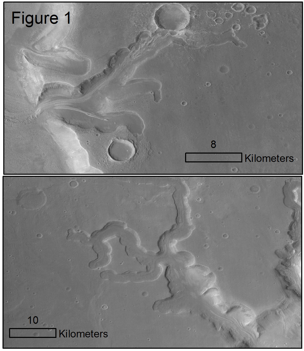
1.1 Research Gaps and Objective
There are studies that focus on the GLFs and their formation over the years (Degenhardt and Giardino, 2003; Holt et al., 2008; Karlsson et al., 2015; Souness et al., 2012). Attempts to date these viscous flow features by studying their composition (Hepburn et al., 2020) have resulted in some progress in understanding Mars' glacial past through these landforms. However, there is still a lack of knowledge of the depths of the GLFs. The reasons for the absence or presence of any buried deposits beneath these landforms are largely uncertain. Although there have been papers targeting these landforms and layers underneath them, there is a requirement to evaluate their complete potential through the extension of radar datasets. Because the undersurface deposits on Mars are mostly dust and dirt (Dundas et al., 2018), detecting them with optical images is difficult. Therefore, this study attempts to examine the depths of glacier-like forms in the mid-latitudes of Mars using SHARAD radargrams.
1.2 Data
The Shallow Subsurface radar instrument on Nasa's Mars reconnaissance orbiter produces very long wavelength radar imagery and can be utilized to detect subsurface layers on Mars. Unlike Earth, ice on the mid-latitudes of Mars sublimates when on the surface and can be found underneath the surface (subsurface). Therefore, to confirm or reject the presence of subsurface deposits on Mars, SHARAD's pulses are used for better penetration of signals into the target landforms. SHARAD’s radar pulses can reach up to 1000-1500 m depth and operate between 15-25 MHz frequencies. The data obtained by the instrument are in the form of radargrams which can be used for geospatial analysis. As shown in figure 2, the radargrams represent power returned at several time delays (Y-axis) along the track of the distance traveled by spacecraft (X-axis) (Bramson and Petersen, 2020). There is an increase in the power (at the time delay) returned from the radar if contrast is realized in the material properties. A material's response can be expressed by dielectric constant or permittivity and is related to the material's refractive index.
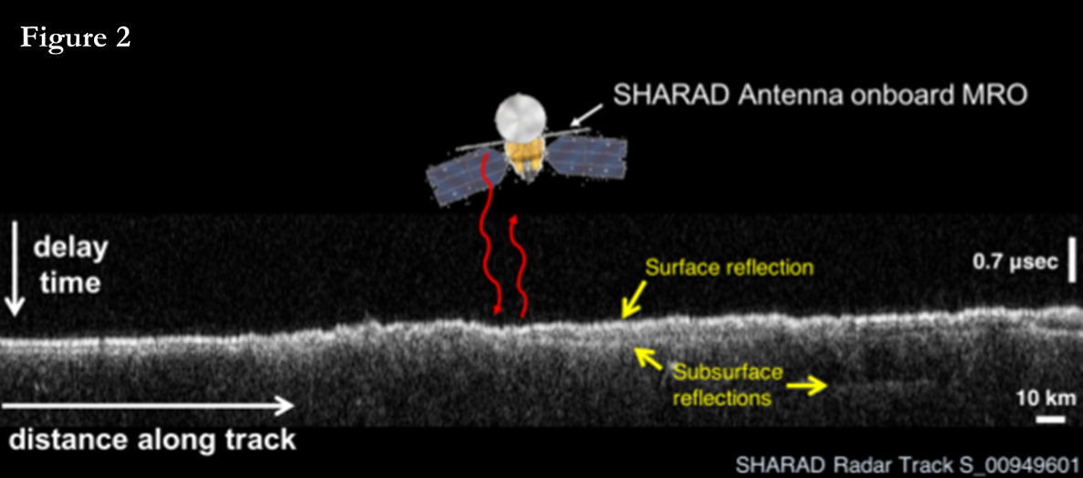
1.3 Methodology
1.3.1 Target glacial-like forms
Most small-scale lobate debris aprons, i.e., features that stretch for less than 5 km, are present in the Northern Lowlands (Hepburn et al., 2020) as shown in figure 3. The selection of a few interesting GLFs is made based on the evidence of hydrous minerals in the area. In the study (Pan and Ehlmann, 2018), Deuteronilus Mensae is closely studied for phyllosilicates and hydrated silica using CRISM images. In this study, the target landforms are selected based on the locations of these hydrous minerals shown in Pan and Ehlmann’s research.
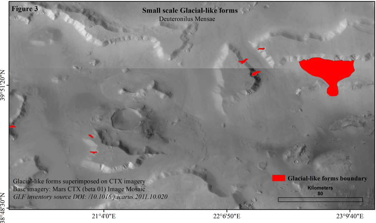
1.3.2 Processing Radargrams
Off-nadir reflections: The performance of the radar sounder is determined by several factors, including surface and subsurface reflectance, receiver noise level, and topography. At longer delays, topographic features away from the nadir track will add undesired noise or "clutter" power (Seu et al., 2007). Therefore, topographical changes can induce different levels of clutter echoes. Bright reflections from off-nadir surface topography cause radar clutter, resulting in late returns that could be misinterpreted for subsurface returns (Bramson et al., 2015). Hence, we compare our radargrams to their respective clutter simulations produced using Mars Orbiter Laser Altimeter.
1.4 Results
In figure 4 original radargram covering a GLF rich in Fe/Mg phyllosilicates in the Deuteronilus Mensae region is shown along with the Themis mosaic indicating the cross-section profile of the radargram. The radargram is compared to a clutter simulation generated using the Colorado SHARAD Processing System. The subsurface reflections can be recognized with the use of clutter simulations. Specific subsurface interfaces are visible in the radargrams directly under the GLFs which are absent in the simulations. This indicates the presence of subsurface deposits under the phyllosilicate-rich GLF.
However, utilizing SHARAD radargrams to look under small-scaled GLFs has inherent difficulties, and due to resolution restrictions, it is difficult to look closely at the radargrams. Deuteronilus Mensae has a complex terrain; hence, in some instances, subsurface reflectors are very similar to the surface reflector caused due to the instrument’s sidelobes (Bramson et al., 2015). Therefore, the radargrams need to be very carefully compared with the simulations to grasp better what can be called a subsurface deposit under the target landforms.
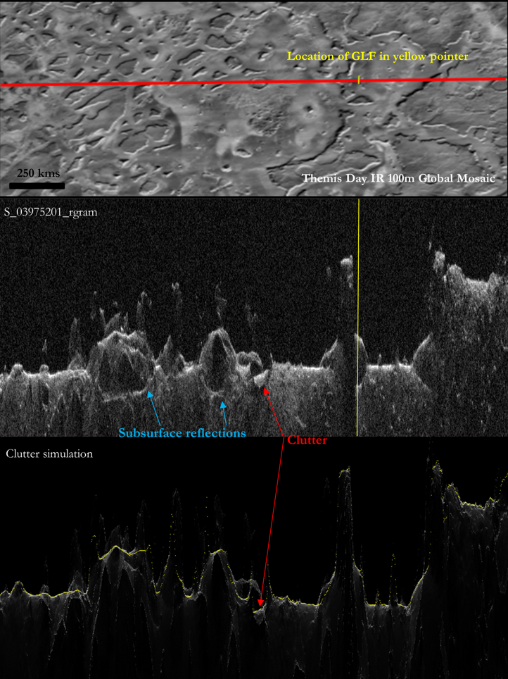
How to cite: Kacholia, D., Bakker, W. H., and Aghababaei, H.: Subsurface layer investigation of the glacial-like forms using SHARAD data, Europlanet Science Congress 2022, Granada, Spain, 18–23 Sep 2022, EPSC2022-382, https://doi.org/10.5194/epsc2022-382, 2022.
Introduction: The Moon exhibits globally dispersed tectonic landforms due to thermal contraction, solid-body tides, and loading of the crust. Wrinkle ridges and lobate scarps are both formed as a result of compressional stresses, however, their appearance and formation mechanisms are different [1-5]. Wrinkle ridges are interpreted as blind thrust faults, where horizontal shortening is accommodated by a fault that does not reach the surface. These faults are suggested to extend to depths between 100’s of meters to several kilometers [6-8]. It is thought that wrinkle ridges formed 0.1-0.65 Ga after basalt emplacement as a result of basin subsidence [6-11]. Lobate scarps on the other hand are among some of the youngest landforms on the Moon, with derived model ages < 700 Ma [12-16]. The faults that created the scarps are thought to offset the upper kilometer of the crust and are predominately in the highlands [15-16]. While wrinkle ridges and lobate scarps are typically not co-located, global mapping revealed at least nine cases where wrinkle ridges transition to lobate scarps at a mare-highland boundary [5,16-18]. These transitions are of interest as they are complex examples of recent tectonism [18-20].
The ridge-scarp transition in eastern Mare Serenitatis (21.7°N, 28.9°E) ruptures the surface at a contact between mare basalts and dark mantle deposits, approximately 70 km NW of the Apollo 17 landing site. The ridge is part of the southern section of the Dorsa Aldrovandi ridge system. Derived model ages for the mare units range from ~3 – 3.8 Ga [21], while the ridge-scarp transition has been active in the last 100 Ma [18]. Detailed mapping around both the ridges and scarp revealed a large network of small-scale graben. To better understand the relationship between the small extensional features and the compressional landforms, a geomorphologic map was produced as a first order investigation.
Data and Methods: We used NAC (Narrow Angle Camera; 1 m/pixel) image data from the Lunar Reconnaissance Orbiter Camera (LROC) with incidence angles of 60-75° for detailed geomorphological mapping [22]. The geomorphologic units and landforms were mapped on the basis of their morphology and albedo (Fig. 1). Wrinkle ridges, lobate scarps and small-scale graben are the mapped tectonic landforms as well as two volcanic units: dark mantle pyroclastic deposits and mare deposits. Impact craters were not included into the map.
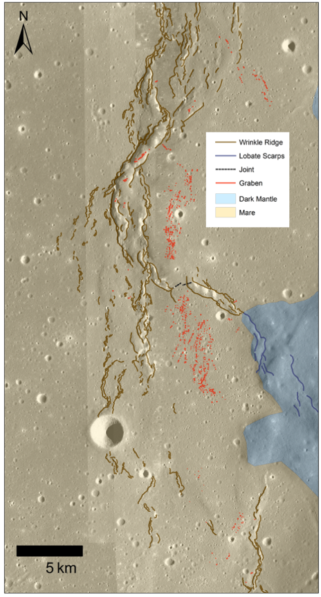
Figure 1: Geomorphologic map of the wrinkle ridge-lobate scarp transition (white arrows) in eastern Mare Serenitatis (21.7°N, 28.9°E) on NAC image data. Brown lines are wrinkle ridge compound scarps, lobate scarps are mapped with blue lines, and small-scale graben are shown with red lines, dashed black lines are joints. Tan color represents the mare, while the light blue areas are dark mantle deposit
Geologic Interpretations (Fig 1.): The wrinkle ridges exhibit typical sinuous and braided morphology [10]. Many ridge sections are discontinuous with some segments as short as 1-2 km in length. The summits of the wider ridge segments occasionally host small-graben that are oriented along strike. Where the ridge crosses the mare-pyroclastic boundary the fault transforms into lobate scarp morphology, likely due to differences in substrate strength and or fault structure. Here, the scarps are simple, curvilinear landforms. The small graben (Fig. 2) are contained within the mare and are mostly tens of meters in length. Graben widths are only a few meters wide and either exhibit typical flat-floors bounded by an escarpment on both sides or v-shaped troughs with irregular edges.
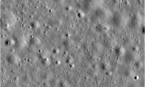
Figure 2: Small-scale graben (21.7º, 28.7º) just south of the ridge section of the transition are approximately perpendicular to the fault.
A smaller ridge, which we tentatively mapped as a joint, traverses the gap (relay ramp) between two segments of the main wrinkle ridge complex and is perpendicular to the main wrinkle complex.
Discussion: Located around the compressional landforms are small-scale graben (Fig. 2). These graben are often found in other locations across the Moon and have been suggested to be the result of localized flexural bending or dilation from recent fault movement at compressional landforms, and are typically found in clusters of ≤20 [23, 24]. However, the graben here occur as a relatively large network (n=991) that spans over ~25 km and they likely formed as a secondary effect (extension) of recent tectonism in the ridges and scarps. These graben have a strong SSW-NNE orientation, which is roughly perpendicular to the section of the wrinkle ridge that transitions into a lobate scarp and parallel to the main Dorsa Aldrovandi ridge. Graben are also observed on the crests of the wrinkle ridges due to extension on the ridge and lateral extrusion of wedge material.
Conclusion: In addition to the late-Copernican ages determined for the wrinkle ridge-lobate scarp transition, the discovery of small-scale graben additionally suggests recent tectonism at the compressional landforms. This supports the hypothesis of a tectonically active Moon [5, 13, 19, 20, 24] that produces not just compressive, but also extensional landforms.
References: [1] Watters & Schultz (2010) Planetary Tectonics, Cambridge Univ. Press. [2] Schultz (1976) Moon Morphology, University of Texas Press. [3] Binder (1982) Earth, Moon, and Planets, 26. [4] Watters and Johnson (2010) Planetary Tectonics, Cambridge Univ. Press. [5] Watters et al. (2010) Science, 329. [6] Schultz (2000) JGR, 105, E5. [7] Solomon and Head (1979) JGR, 84. [8] Watters (1993) JGR-Planets, 98. [9] Solomon and Head (1980) Rev. Geophys. Space Phys., 18. [10] Plescia and Golombek (1986) GSA Bull., 97. [11] Yue et al. (2017) LPSC, #1926. [12] Binder and Gunga (1985) Icarus 63. [13] van der Bogert et al. (2018) Icarus 306. [14] Clark et al. (2015) LPSC, #1730. [15] Clark et al. (2016) LPSC, #1380. [16] Watters et al. (2015) Geology 43, 10. [17] Thompson et al. (2017) LPSC, #2665. [18] Clark et al (2019) LPSC, #2084 [19] Clark et al. (2017) LPSC, #1001. [20] Williams et al (2019) Icarus 326. [21] Hiesinger et al. (2000) JGR, 105. [22] Robinson et al. (2010) Space Sci. Rev. 150. [23] Watters et al (2012) Nature Geo. Sci. 5. [24] French et al (2015) Icarus 252.
How to cite: Clark, J. D., Bernhardt, H., and Robinson, M. S.: Extensional Features at East Serenitatis Wrinkle Ridge-Lobate Scarp Transition Indicate Recent Tectonic Activity, Europlanet Science Congress 2022, Granada, Spain, 18–23 Sep 2022, EPSC2022-757, https://doi.org/10.5194/epsc2022-757, 2022.
The increasing availability of radar sub-surface/surface imaging of the terrestrial planets allowed to highlight the structural architecture of buried geological structures. The reconstruction of the 3D subsurface geometries, besides supporting the classic geologic mapping of planetary surfaces, allows to constrain models to unravel the 4D evolution of a region. This is of utmost importance in key regions where trapped subsurface fluids and their (possible) migration to the surface might impact local/global climate conditions , atmospheric composition, as well as the presence of water close to the maritan surface.
Shallow Subsurface Radar (SHARAD) data [1] revealed that the Martian caps are composed primarily of water ice that was deposited in layers that contain varying amount of dust. They are referred to as martian Polar Layered Deposits (PLD). The internal stratigraphy of these deposits strongly resemble the internal layering in key sites of the East Antarctic Ice Sheet, where the ice tectonics (e.g. ice faulting) and dynamics, revealed to be the causes of the observed architecture.
Mechanisms responsible for the formation and evolution of the martian PLD are still under debate and exogenous processes are considered among the best candidates [2]. Steep troughs dissecting the polar ice caps with spiral shapes provide an optimal view of the layered internal structures. Ice reflectors interpretations suggested a migration of these troughs accompanied by katabatic winds that produce erosion/sublimation at the exposed layers and accumulation/deposition at the opposite slopes [2]. Nevertheless, the SHARAD profiles crosscutting these canyons revealed the lateral change in thickness of ice layers, with thickening as they approach the canyon structures (Fig.1). It is well known from the terrestrial analogues/structures that such geometry may well result from the activity of normal faults with sintectonic sedimentation (ice and dust deposition in the martian case).
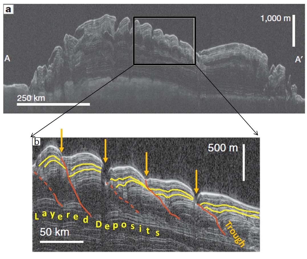
Figure 1. Sharad Image showing examples of the stratigraphic architecture of the North Polar Layered Deposits and spiral through dissecting the ice cap.
In this work we present the results the forward numerical modeling by HCA technique [3] of the PLD structure evolution.. The layered ice is simulated by a mesh of cells whose links replicate the physical and rheological characteristics of the material as well as the presence of ruptures such as faults. The observed ice stratigraphy of the PLD, the lateral thickness variations, and their vertical offset are successfully simulated through the activity of shear discontinuities with a series of listric shapes and normal displacements (Fig.2).
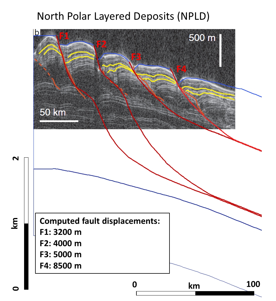
Figure 2. HCA numerical model of the ice layered deposits from Mars north polar region. Subset of SHARAD radargram 1294501 [3]
The HCA kinematic modeling thus revealed the existence faults with size of the order of hundreds of km within the Martian ice caps. Faults with similar size and displacement of the order of several kms are associated with well developed and extended fault core and damaged zones, characterized by strong variation in permeability due to secondary fracturing. In this way the martian ice cap faults produce corridors of brittle deformation that dissect the entire ice cap, provide conduits for fluid migration, and enhance the development of the observed troughs.
The width of the fault damaged zones is of the order of the hundreds of meters and the presence of the fault core, the attitude of fault-related fractures (synthetic fractures, antithetic fractures, extensional fractures, pressure solutions seams) and their spatial distribution and frequency in the ice volume affected by the damage zone of the shear discontinuities has been quantified by the analytical-numerical modeling performed with FRAP software using the found fault geometry [4]. This model takes into account the kinematic conditions of the modeled fault, the physical properties of the ice material and environmental parameters (e.g. acting stresses, gravity, fluid pressure …) which influence the computation of the secondary permeability (Fig 3).
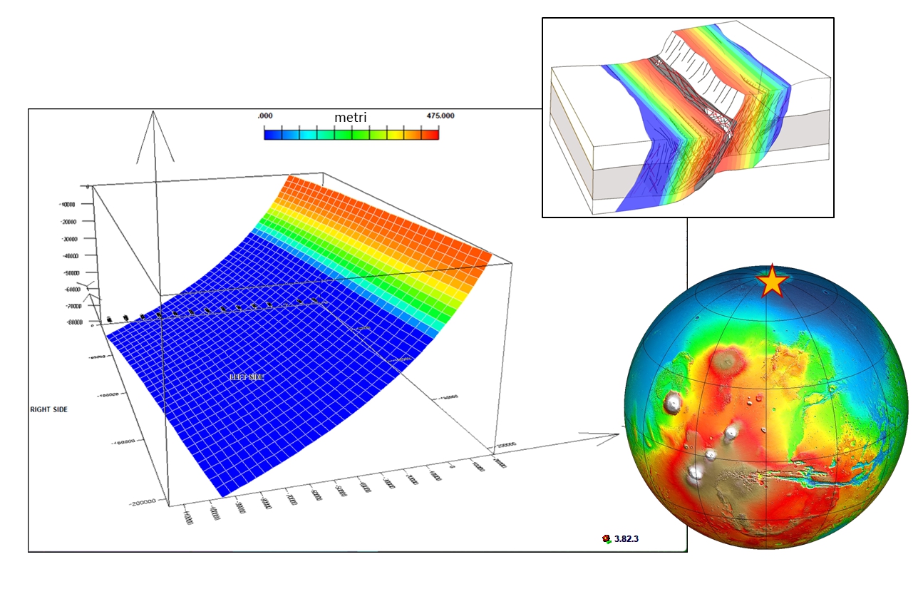
Figure 3. Schematic 3D sketch showing the ice volume affected by fault-related fractures and the development of secondary permeability in the fault damage zone (example of FRAP output).
Results of this study represent a contribute to better understand the hitherto underestimated ice tectonic setting of the Martian ice caps. Highlighting the hydraulic properties of these faults is pivotal to understand the enhanced pathway of fluid that are trapped both within the ice layers and at the base of the ice caps. Fluids and biological material can thus approach the surface and the atmosphere and may be easily detectable/sampled to improve the success of future onland missions.
References
[1] Seu, R., Biccari, D., Orosei, R., Lorenzoni, L. V., Phillips, R. J., Marinangeli, L., ... & Zampolini, E. (2004). SHARAD: The MRO 2005 shallow radar. Planetary and Space Science, 52(1-3), 157-166.
[2] Smith, Holt, Spiga, Howard, Parker (2013). The spiral troughs of Mars as cyclic steps. Journal Of Geophysical Research: Planets, 118, 1835–1857.
[3] Salvini F. Storti F., McClay K (2001)) Self-determining numerical modeling of compressional
fault-bend folding. Geology, 29, 839-842.
[4] Salvini F. (2005). FRAP – Fault-Related fracturing by Analytic-numerical aPpproach. Inhouse developed application at the GEoQuTe Lab, Roma Tre University.
How to cite: Cianfarra, P., Salvini, F., Balbi, E., and Maggi, M.: Structural glaciology of the Martian ice caps unveils conduits for fluid migrations, Europlanet Science Congress 2022, Granada, Spain, 18–23 Sep 2022, EPSC2022-844, https://doi.org/10.5194/epsc2022-844, 2022.
TP12 | Planetary Seismology and Geophysics
The InSight (Interior Exploration using Seismic Investigations, Geodesy and Heat Transport) lander is providing an unprecedented set of high frequency records of ground deformations, pressure and wind at the surface of Mars. Seismic and acoustic waves from impacts have been observed by SEIS seismometer through the ground movements that they generate, and their sources as impacts have been confirmed with orbital images of newly appearing craters. Three impacts have been identified and located, and one additional seismic event is consistent with a date-constrained new impact. Several other events are currently being investigated as well. Arrival times and polarization of seismic and acoustic waves were used to estimate impact locations. These estimated locations were subsequently confirmed by orbital imaging of associated craters and temporal matches to the events times, with previous orbital images showing no craters. Crater dimensions and estimates of meteoroid trajectories from images allow us to understand and model the recorded seismograms. The precise source locations provided by impacts as compared to tectonic sources provide direct constraints on the structure of the martian interior. First arrival seismic waves confirm the previously determined crustal models, and the dispersion of trapped acoustic waves confirms the current models of sound speed and wind in the atmosphere. In addition, these observations provide the first ground-truth for distance-amplitude scaling relationships between impacts and the mechanical waves for Mars. They confirm the relationship between the seismic moment of impacts and the vertical impactor momentum, and demonstrate the capability of planetary seismology to constrain impact rates and internal structure of terrestrial planetary objects throughout the solar system.
How to cite: Garcia, R. F. and the InSight and CTX science teams: First seismo-acoustic location and orbital imaging of recent impacts on Mars: constraints on atmosphere and interior structure and impact processes, Europlanet Science Congress 2022, Granada, Spain, 18–23 Sep 2022, EPSC2022-10, https://doi.org/10.5194/epsc2022-10, 2022.
The Interior Exploration using Seismic Investigations, Geodesy and Heat Transport (InSight) mission has discovered over thirteen hundreds seismic events since landing on Mars in 2018, shedding the light on the internal structure of Mars (InSight Marsquake Service, 2022). These events have been applied in various Martian seismology studies such as interiors determination and scattering estimation (Lognonné et al., 2020). Site effect study, which is commonly conducted on Earth to estimate the seismic hazard and invert the surficial subsurface structure, has been implemented to Martian ambient noise and event records (Carrasco et al., 2022; Xiao et al., 2022). Nevertheless, a recently detected big event S1222a that reach the magnitude of about 5.0 would further aid to the site effect study beneath the landing site. The amplification of ground accelerations is thought to be related to the subsurface layers and mostly event-independent. Therefore, site effects from different events are expected to share similar features and help to obtain a better result with lower uncertainty compared to result from single event.
The main focus of this study is to investigate the subsurface resonances excited by seismic events in high frequencies above 1.0 Hz. We adopted the classical horizontal to vertical spectral ratio (HVSR) method (Nakamura, 1989) and coherency analyses and explored the optimal parameters for these time-frequency analyses in order to balance both time and frequency resolutions. We used the ambient noise to serve as a baseline in order to distinguish the effects of seismic events and environmental contaminations. Results from ambient noise show that the HVSR spectrogram and coherogram are consistent to each other and both show diurnal variation controlled by the local meteorological conditions. Several H/V peaks are found in the averaged H/V curve, most likely originating from the wind-induced lander vibrations. In contract, we calculated the H/V curves within the P-wave and S-wave windows provided by InSight Marsquake Service (2022) to compare with the results from ambient noise. S1222a stands out to exhibit abundant high frequency content well above the noise level, while other events present energy close to noise level for frequencies above 5.0 Hz. Besides, we identified the excitation of lander modes by seismic events, which is most obvious for the magnitude ~5 S1222a event perhaps due to its very high signal-to-noise ratio. All the analyses above indicate the existence of site effects and both subsurface and lander mechanical resonances could be excited. It is thus important to study how to separate the subsurface resonances and further use them for sublayer inversion.
Previous studies from InSight hammering experiments and jointly seismic-geodetic inversion obtained the physical properties of surficial regolith (Lognonné et al., 2020). Together with these results, it is possible to better constrain the very shallow layers beneath the landing site. Since the site effects would basically have influence on all observation of InSight seismic data, this study also has implication to environmental contamination removal, sublayer velocity inversion, and any other seismic studies that could be affected by strong site effects.
References
[1] Carrasco, S., et al. (2022). Empirical H/V spectral ratios at the InSight landing site and implications for the martian subsurface structure. Geophysical Journal International, submitted.
[2] Lognonné, P., et al. (2020). Constraints on the shallow elastic and anelastic structure of Mars from InSight seismic data. Nature Geoscience, 13(3), 213-220. https://doi.org/10.1038/s41561-020-0536-y
[3] InSight Marsquake Service (2022). Mars Seismic Catalogue, InSight Mission; V10 2022-04-01. ETHZ, IPGP, JPL, ICL, Univ. Bristol. https://doi.org/10.12686/a16
[4] Nakamura, Y. (1989). A method for dynamic characteristics estimation of subsurface using microtremor on the ground surface. Railway Technical Research Institute Quarterly Report, 30(1), 25–33.
[5] Xiao, W., et al. (2022). Characteristics of Horizontal to Vertical Spectral Ratio of InSight Seismic Data from Mars. Journal of Geophysical Research, under review.
How to cite: Xiao, W., Lognonné, P., Kawamura, T., Xu, Z., Carrasco, S., and Knapmeyer-Endrun, B.: Site Effect Study based on Magnitude 4~5 InSight Marsquakes, Europlanet Science Congress 2022, Granada, Spain, 18–23 Sep 2022, EPSC2022-816, https://doi.org/10.5194/epsc2022-816, 2022.
We report the results of more than 2 years of monitoring the rotation of Mars with the RISE instrument on InSight. Small periodic variations of the spin axis orientation, called nutations, can be extracted from the Doppler data with enough precision to identify the influence of the Martian fluid core. For the first time for a planetary body other than the Earth, we can measure the period of the Free Core Nutation (FCN), which is a rotational normal mode arising from the misalignment of the rotation axes of the core and mantle. In this way, we confirm the liquid state of the core and estimate its moment of inertia as well as its size.
The FCN period depends on the dynamical flattening of the core and on its ability to deform. Since the shape and gravity field of Mars deviate significantly from those of a uniformly rotating fluid body, deviations from that state can also be expected for the core. Models accounting for the dynamical shape of Mars can thus be tested by comparing core shape predictions to nutation constraints. The observed FCN period can be accounted for by interior models having a very thick lithosphere loaded by degree-two mass anomalies at the bottom.
The combination of nutation data and interior structure modeling allows us to deduce the radius of the core and to constrain its density, and thus, to address the nature and abundance of light elements alloyed to iron. The inferred core radius agrees with previous estimates based on geodesy and seismic data. The large fraction of light elements required to match the core density implies that its liquidus is significantly lower than the expected core temperature, making the presence of an inner core highly unlikely. Besides, the existence of an inner core would lead to an additional rotational normal mode the signature of which has not been detected in the RISE data.
How to cite: Rivoldini, A., Le Maistre, S., Caldiero, A., Yseboodt, M., Baland, R.-M., Beuthe, M., Van Hoolst, T., Dehant, V., Folkner, W., Buccino, D., Kahan, D., Marty, J.-C., Antonangeli, D., Badro, J., Drilleau, M., Konopliv, A., Peters, M.-J., Plesa, A.-C., Samuel, H., and Tosi, N. and the InSight/RISE team: A view into the deep interior of Mars from nutation measured by InSight RISE, Europlanet Science Congress 2022, Granada, Spain, 18–23 Sep 2022, EPSC2022-1101, https://doi.org/10.5194/epsc2022-1101, 2022.
TP13 | Planetary Dynamics: Shape, Gravity, Orbit, Tides, and Rotation from Observations and Models
1) Introduction
In the context of the Artemis program, the interest of lunar study has been renewed. The Lunar Laser Ranging (LLR) experiment allows since fifty years to determine the Earth-Moon distance at a few centimeters accuracy and the Moon’s librations at a one milliarcsecond accuracy ([4], [3]) Such accuracy allows a refined description of the Moon’s rotation.
The tidal response of the Moon depends on its density and rheology and it affects its rotation. Therefore it provides important information on the lunar internal structure (e.g. [6], [7], [5], [1]). The variation of the harmonic degree 2 gravitational potential due to the tidal response can be quantified by the tidal Love number k2. The latter depends on the forcing frequency, which are mainly exerted by the Earth and the Sun. The dissipation is quantified by the dissipation factor Q which is related to the value of the time delay.
2) Time-delay lunar tides
Furthermore, because of the dissipation due to the viscosity of the lunar interior, the tidal deformation is not instantaneous. The current version of the planetary and lunar ephemeris INPOP only account for unique k2 and time delay [4]. Time delay can be described by a complex Love number k2, which in this case, depends also on the forcing frequency [7]. The dissipation factor Q is related to the imaginary part of the Love number.
Here we explore the introduction of tidal models in numerical ephemerides. We aim to include the k2 and Q frequency dependency in INPOP.
The formulation in Fourier series of the distortion coefficients (also called variation of the Stokes coefficients) by Williams and Boggs (2015) ([7]) allows to describe the tidal gravitational variation in accounting for the frequency dependency of the complex k2. The distortion coefficients vary according to the forcing frequencies formulated as linear combinations of the Delaunay arguments, the latter being described as a polynomial expansion with respect to the time.
3) Representation of the orbit of the Moon
However, the representation in series of the distortion coefficients needs to be consistent with the ephemerides that we use. For that, we can use a semi-analytical representation of the ephemerides.
Numerical ephemerides can described the orbit and the rotation of the Moon with a good accuracy according to the observational error. In complement, the semi-analytical approach is useful to extract information and to disentangle the different physical contributions contains in the numerical approaches. The Éphéméride Lunaire Parisienne (ELP) provides the most accurate semi-analytical model of the orbital motion of the Moon, in the form of Fourier and Poisson series [2].
Figure 1 shows that the difference of the Earth-Moon distance between the solution of INPOP19a and the solution of ELP fitted to INPOP19a reach a maximum value of the order of 4 m. Then, we deduce the amplitude of the distortion coefficients from the fitted semi-analytical representation.

Figure 1. Difference of the Earth-Moon distance between the solution of IN- POP19a and the solution of ELP fitted to INPOP19a. The origin of time is J2000.
References
[1] A. Briaud, A. Fienga, D. Melini, N. Rambaux, A. M ́emin, G. Spada, C. Sal- iby, H. Hussmann, and A. Stark. Constraints on the Moon’s Deep Interior from Tidal Deformation. In LPI Contributions, volume 2678 of LPI Contri- butions, page 1349, March 2022.
[2] J. Chapront and G. Francou. The lunar theory ELP revisited. Introduction of new planetary perturbations. , 404:735–742, June 2003.
[3] Ryan S. Park, William M. Folkner, James G. Williams, and Dale H. Boggs. The JPL Planetary and Lunar Ephemerides DE440 and DE441. , 161(3):105, March 2021.
[4] V. Viswanathan, A. Fienga, O. Minazzoli, L. Bernus, J. Laskar, and M. Gastineau. The new lunar ephemeris INPOP17a and its application to fundamental physics. , 476(2):1877–1888, May 2018.
[5] V. Viswanathan, N. Rambaux, A. Fienga, J. Laskar, and M. Gastineau. Observational Constraint on the Radius and Oblateness of the Lunar Core- Mantle Boundary. , 46(13):7295–7303, July 2019.
[6] James Williams, Dale Boggs, Charles Yoder, James Ratcliff, and J. Dickey. Lunar rotational dissipation in solid body and molten core. Journal of Geo- physical Research, 106:27933–27968, 11 2001.
[7] James G. Williams and Dale. H. Boggs. Tides on the Moon: Theory and determination of dissipation. Journal of Geophysical Research (Planets), 120(4):689–724, April 2015.
How to cite: Baguet, D., Rambaux, N., Fienga, A., Mémin, A., Briaud, A., Hussmann, H., Stark, A., Hu, X., Viswanathan, V., and Gastineau, M.: Introduction of tidal models in lunar ephemerides, Europlanet Science Congress 2022, Granada, Spain, 18–23 Sep 2022, EPSC2022-978, https://doi.org/10.5194/epsc2022-978, 2022.
Ejection of solid bodies from comets and its dynamical significance for velocity and rotation of comet
Introduction
Observations of comets 9P/Tempe 1 and 67P/Churyumov – Gerasimenko revealed existence of several ejections of significant masses [1, 2, 3].
In the present paper we investigate dynamic effects for the comet of similar ejections. Contrary to research presented in [6], we consider here ejections with higher velocity, i.e., 0.71 m s-1 or higher from different places mainly on the surface of the comet 67P/Churyumov – Gerasimenko and some our model body.
Gravitational field and mechanism of ejection
The gravitational field of considered comet is complicated [1, 4]. There are several regions of different slopes of the comet's surface in respect to the local gravity. Note also non-spherical shape of cometary surface of constant potential [6].
In [6] there are considered slow ejecta (i.e. ejecta with velocity below escape velocity). Here we consider the ejecta with the velocity 0.71 m s-1 or higher. Often, the initial velocity is higher than the escape velocity. Note, however, that the for comets of irregular shape, the escape velocity depends strongly on the site of ejection.
A following model of processes leading to the ejection is assumed. It is based on [3, 4]. The phase changes supply the heat to a certain underground volume. If the pressure exceeds some critical value then some fragments will be ejected into space. Many places in the comet could be a result of such processes [3]. Note that the initial velocity of ejecta are assumed to be perpendicular to the physical surface. This assumption is used successfully in [4].
Calculations
We consider ejecta from different places on comet 67P/G-C. For the comet dynamical effects of slow ejecta is more limited but also more complicated because the comet obtained back some momentum and spin from the landing ejecta.
We performed calculations for 530 ejected particles from different places in the comet 67P/C-G and some for our model body. Total mass of ejecta for the comet 67P is chosen to be: 10-6 or 10-5 of the mass of the whole comet. These values correspond to ~105 kg and ~106 kg for each ejected particles (it depends on the number of particles used for given calculation). The following velocities of ejecta are used: 0.7, 1.0, 10 m s-1. Other values are used for the model body. For calculations the program developed by L. Czechowski was used.
Preliminary results and conclusions
In general, the effect of ejecta on comet's motion is primarily determined by the total momentum and angular momentum of the ejected particles. However, unlike the gases ejected by comet jets, the movement of solid particles depends heavily on the comet's gravitational field. The solid particles can return to the comet, giving up some of their momentum. Therefore, they have a different effect on comet motion and should be taken into account in more accurate calculations of comet's motion.
Acknowledgements
The research is partly supported by Polish National Science Centre (decision 2018/31/B/ST10/00169)
References
[1] Czechowski L., (2017) Dynamics of landslides on comets of irregular shape. Geophysical Research Abstract. EGU 2017 April, 26, 2017
[2] Jorda, L., R. et al. (2016) The global shape, density and rotation of Comet 67P/Churyumov-Gerasimenko from preperihelion Rosetta/OSIRIS observations, Icarus, 277, 257-278, ISSN 0019-1035, https://doi.org/10.1016/ j.icarus.2016.05. 002.
[3] Kossacki K., Czechowski L., 2018. Comet 67p/Churyumov–Gerasimenko, possible origin of the depression Hatmehit. Icarus vol. 305, pp. 1-14, doi: 10.1016/j.icarus.2017.12.027
[4] Czechowski L. and Kossacki K. J. 2021. Dynamics of material ejected from depression Hatmehit and landslides on comet 67P/Churyumov–Gerasimenko. Planetary and Space Science 209, 105358, https://doi.org/10.1016/j.pss.2021. 105358
How to cite: Czechowski, L.: Ejection of solid bodies from comets and its dynamical significance for velocity and rotation of comet, Europlanet Science Congress 2022, Granada, Spain, 18–23 Sep 2022, EPSC2022-1029, https://doi.org/10.5194/epsc2022-1029, 2022.
The classical approach to estimate an asteroid's mass is to analyze its gravitational interactions with another object such as a spacecraft, Mars, a companion asteroid, or a separate asteroid during an asteroid-asteroid close encounter. The latter case leads to gravitational perturbations on a small, generally assumed massless, test asteroid, by the larger perturber asteroid involved in the encounter. By measuring and modeling these perturbations it is possible to estimate the mass of the larger asteroid. This can be described as an inverse problem where the aim is to fit six orbital elements for each asteroid in addition to masses for the perturbing asteroids into astrometric data for each asteroid.
Given that the signals of the perturbations are generally very weak, high precision astrometry and long observational arcs are vital for estimating asteroid masses with acceptable accuracy. It follows that the milliarcsecond-precision astrometry produced by the Gaia spacecraft is a great boon to the field and asteroid mass estimation is considered one of the main applications of Gaia's Solar System Object (SSO) astrometry (Gaia Collaboration et al. 2018a). Indeed, we have recently demonstrated that usage of SSO astrometry from the second Gaia Data Release (DR2) (Gaia Collaboration et al. 2018b) in combination with Earth-based astrometry can reduce the associated uncertainties by up to an order of magnitude in comparison to results computed with Earth-based alone (Siltala & Granvik 2022). In that work, we observed that DR2 does remain limited by the relatively short observational arc of the astrometry as well as the low number (14,099) of asteroids included, which excludes a large number of potentially interesting asteroids.
The third Gaia Data Release (DR3), to be released in June 2022, is expected to remedy these issues to a certain extent. DR3 will include astrometry approximately 11 times more asteroids (158,152) over a much longer timespan. In addition, the SSO data processing has improved and correspondingly we expect further improvements in data quality. Thus, DR3 will enable a large number of asteroid mass estimates beyond what is already possible with DR2 while leading to further improvements to the uncertainties of the masses in cases where DR2 was already usable.
In this presentation, we demonstrate the practical impact of DR3 on asteroid mass estimation. We re-compute asteroid masses from several test cases we previously studied with Gaia DR2 and compare the results to those previously obtained in Siltala & Granvik 2022. Both mass estimation with DR3 alone and in combination with Earth-based astrometry are attempted. Such comparisons will reveal the extent of the improvements to asteroid masses enabled by DR3.
Finally, we briefly discuss future prospects for the application of DR3 to mass estimation, including a comprehensive study of a much larger sample of asteroids,
References
Gaia Collaboration, Spoto, F., Tanga, P., Mignard, F., and 621 co-authors (2018a). Gaia Data Release 2. Observations of solar system objects. A&A, 616:A13.
Gaia Collaboration, Brown, A. G. A., Vallenari, A., Prusti, T., and 621 co-authors (2018b). Gaia Data Release 2. Summary of the contents and survey properties. A&A, 616:A1.
Siltala, L. and Granvik, M. (2022). Masses, bulk densities, and macroporosities of asteroids (15) Eunomia, (29) Amphitrite, (52) Europa, and (445) Edna based on Gaia astrometry. A&A, 658:A65.
How to cite: Siltala, L. and Granvik, M.: Asteroid Mass Estimation with the Third Gaia Data Release, Europlanet Science Congress 2022, Granada, Spain, 18–23 Sep 2022, EPSC2022-1081, https://doi.org/10.5194/epsc2022-1081, 2022.
TP14 | Impact Processes in the Solar System
1. Introduction
Previous studies of resurge sediments from several marine-target impact craters indicate a relationship between the sedimentology, , the target water depth, H, and the magnitude of the event, d. This offers a valuable opportunity to obtain one of these variables if the other two are known. However, the mechanisms controlling this relationship have not been unraveled yet. During the cratering process fragments from the solid target are mixed with the seawater and, after an initial turbulent phase, they get deposited inside the seafloor crater when filled up by the resurging water. We present a mathematical model for the aquatic settling process of the resurge material as a feasible explanation for the observational data.
2. Methods
2.1. Fractal model for particle settling
The impact-related sediments considered here are formed from primary fragmented material, giving rise to a distribution of particles and aggregates that can be interpreted as a cumulative function. Thus, for the study of the particle settling a fractal model is considered [1][2].
In this study, we assume that size segregation is correlated to the concentration of the solid particles [3][4] giving rise to the different settling patterns observed in the core samples. The density and viscosity of the solid/water mixture depend on the solid concentration causing a different settling velocity of the particles. For low concentrations, velocities of coarse particles are higher and fine particles are excluded from the lower part of the sediment, while for high values of the concentration the settling of the coarse clasts become hindered by the higher concentration of fine grains in the solid/water mixture, thus reducing the packing of coarse fragments at the bottom of the sediment column.
In order to analyze the size segregation effect, Herreros and Ormö [5] proposed a fractal model in two steps, considering the settling process of two types of particles: (1) Fine particles, s; and (2) coarse particles, p, with radius Rp > Rs, taking the settling time for the coarse particles in pure water as a time reference (tmax):
Step 1: Settling of fine particles in pure water. The suspended mass fraction of fine particles, s, in pure water is calculated. At this step, the settling of the fine particles is considered independent on the solid/water concentrations.
Step 2: Settling of coarse particles in a solid/water mixture. In this case, the coarse particles, p, are assumed to be immersed in a fluid mixture whose viscosity and density are both functions of the volumetric concentrations.
According to [5], the number of settled coarse particles per unit length, i.e. the mean clast frequency , can be approximated by:

where Rm is the average size of the coarse particles and lds and ldp are the heights of an equivalent cylindrical volume of deposited mass.

2.2. Application to marine impacts
After a meteorite impact, the transient crater diameter, Dt, can be related to the impactor diameter, d [6]. Considering the height of excavated material [7], Hexc = Dt/10, as a solid/water mixture column, HT = Hexc = Hs+Hw, the impactor diameter, d, can be expressed as:

where standard values for impactor’s velocity, density and impact angle have been considered [8][9]:

2.3. Mass excess
The effect of the relative fraction of external mass apported to the system, δ, of different origin to the target fragmentation, can be evaluated by just considering the new values for the volumetric concentrations:

which involves an increase in the concentration of solids.
3. Results
As shown in [5], it is possible to represent as a function of d/Hw (in the following just d/H) since both are functions of the solid/water concentrations.
As a result, we obtain a family of curves depending on two parameters: the suspended mass of solid material when all the particles with r > Rp have been settled (i.e. t= tmax), and the excess of solid material apported to the system (Figure 1).
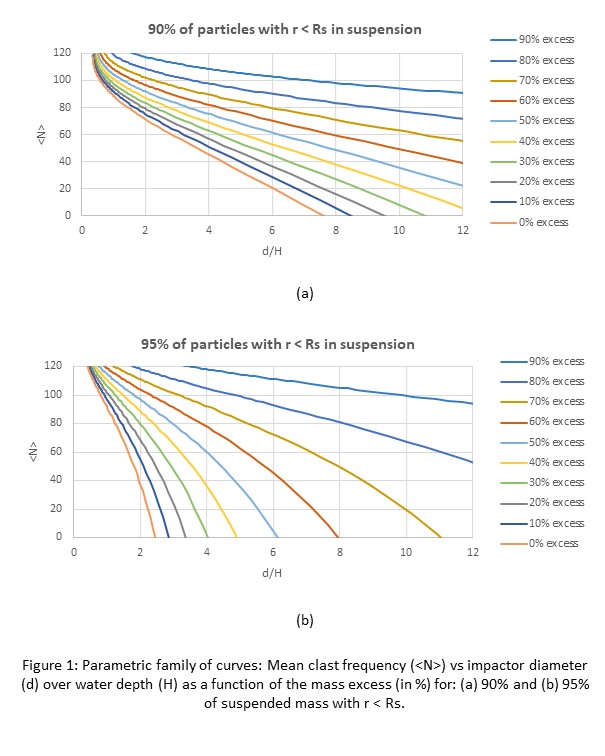
4. Discussion
In order to understand the physics behind the relationship observed in [10], the proposed model has been applied. Figure 2 shows the model results along with the nine drill cores extracted from seven natural impact craters.

The presented model allows the physical interpretation of the observational data, providing a better understanding of the settling conditions. According to the model, the lower position curve (orange curve) represents stable settling conditions, closer to slack-water along with a null excess of mobilized material. This ideal situation, predicted by the model, is compatible with the position and characteristics of the related drill cores. However, the cases laying on the high position curve (blue curve) are those mobilizing a larger amount of solid material and with a higher depositional time for the finest particles, probably related to turbulent flow conditions during the settling process [10].
5. Conclusions
A fractal model for the study of size segregation and particle settling after an impact event in a marine target is presented. The model explains the observed tendency for nine cores obtained from seven natural impact craters, shedding light on the physical processes behind the observations.
Acknowledgements
The authors would like to gratefully acknowledge CSIC financial support for i-LINK project LINKA20203 and to the AEI for project MDM-2017-0737.
References
[1] Filgueira et al., Soil Sci. Soc. Am. J. 67, 1703–1706, 2003.
[2] Filgueira et al., Geoderma 134, 327–334, 2006.
[3] Snabre et al., Rheol Acta 48, 855–870, 2009.
[4] Spearman and Manning, Ocean Dynamics 67, 465–483, 2017.
[5] Herreros and Ormö, EPSC2020-931, 2020.
[6] Johnson et al., Icarus 271, 350–359, 2016.
[7] Melosh, Impact Cratering: A Geologic Process. Oxford University Press Inc, USA, 1989.
[8] Shoemaker, San Diego: Academic Press, 283–359, 1962.
[9] Shoemaker, New York: Pergamon Press, 617–628, 1977.
[10] Ormö et al., Earth and Planetary Science Letters, Vol. 564, 116915, 2021.
How to cite: Herreros, I. and Ormö, J.: Magnitude of marine impacts: Size segregation patterns as an observational assessment., Europlanet Science Congress 2022, Granada, Spain, 18–23 Sep 2022, EPSC2022-41, https://doi.org/10.5194/epsc2022-41, 2022.
INTRODUCTION
The Tabernas Basin (Betic Cordillera) is filled with Neogene, Pliocene and Pleistocene sediments, discordant on a metamorphic basement (Fig. 1). During the Tortonian sedimentation an up to 70 m thick bed of breccia (the Gordo Megabed) was deposited. It consists of up to several tens of meters large, rotated sedimentary megablocks frequently capped and/or surrounded by a polymict breccia of mainly up to m-sized clasts of the crystalline (schist) basement. Previous workers have suggested the bed to be a seismite. The polymict composition of the studied breccias intercalated within the otherwise shallow-marine sediments, the presence of megablocks, plastically deformed megablocks and shock metamorphic features in quartzs of polymict breccias have led us to the description and reinterpretation of sediments and geomorphological features in the Tabernas Basin that could be related to an impact structure.
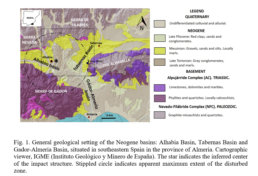
MATERIALS AND METHODS
Multiple field studies were carried out over the course of several years to study the geology and geomorphology of the Tabernas Basin and its surroundings with special focus on the Gordo Megabed. These studies were carried out in conjunction with geological mapping and the measurement of parameters of the observed geological structures.
Thin sections (97 in total) from the different lithologies and locations were prepared and studied for shock metamorphic features under an optical microscope. Quartz grains displaying planar features were studied using the techniques described in Stöffler and Langenhorst (1994) and Ferrière et al. (2009).
RESULTS
Megablocks
We define megablocks as coherent rock blocks that are tilted or rotated, lithologically homogeneous, and that extend in outcrops over at least 30 meters (i.e. having dimensions of several tens of meters).
The material of the megablocks is often made up of sets of turbidites belonging to the Gordo Megabed and three zones have been identified and mapped:
- Zone 1: Central part of the Neogene basin of Tabernas (Rambla de Tabernas).
- Zone 2: Borders to zone 1 to the east and features such as Cerro Alfaro.
- Zone 3: Neogene basin of Alhabia, on the northern flanks of Sierra de Gador.
Plastically Deformed Megablocks
Only three outcrops of these structures SB1, SB2 and SB3 (Fig. 2). They involve recumbent folds with reverse limb whose fold axes follow the direction: N25E, N275E and N210E. They represent plastic internal deformation of the within the slump unit mobilized stacks of Late Tortonian turbiditic marl and sandstones beds, inclined to the NE, W and SW and their directions do not match the main tectonic structures that formed these Neogene basins E-W to NE-SW (Martínez et al., 2017).
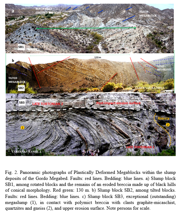
Polymict breccias
Most of the polymict breccias studied (28 in total) are located at the Rambla de Tabernas and present a single lithostratigraphic, mainly graphite-micaschist, quartzite and gneiss, as well as brecciated dolomite. These breccias are massives, unstratified, clast supported and lacks visible sedimentary structures. The angular shape of the fragments indicates short transport, but the basement clast lithologies of the breccia originates far from the present locations.
Breccia 29 is in an anomalous stratigraphic position on Triassic phyllites in Sierra Alhamilla. This is a variable 10-50 cm thick deposit of Neogene material (loams, sands and limestones).
Breccia 30 (sample 2) is located in Sierra de Gádor and constitutes an intermixture of different materials, from both the metamorphic substrate and the Neogene sedimentary sequence.
These features in both breccias could be compatible with a proximal ejecta layer and may clearly be identified by the presence of shock-metamorphic features (Osinski et al., 2013).
Shock-metamorphic features
The systematic search for quartz grains with shock metamorphic features in breccias, resulted in six quartz grains, five grains displaying one set of planar features and one grain with two sets. The features are straight, parallel, sets of planes with a typical spacing between each plane of 1-5 μm. The planar features penetrate the entire grain in four cases, and in two cases they were only visible near the grain boundary in part of the host grain. The features are generally fresh, but occasionally decorated, i.e., lined by minute fluid inclusions (Fig. 3).
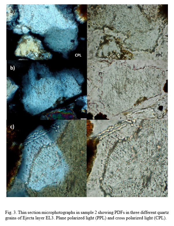
Nevertheless, in light of the indicative, albeit not affirmative, presence of a shocked quartz grains in what we find as analogous lithologies to known impactites based on their composition, appearance, stratigraphic position and geographical distribution, as well as the other sedimentological, stratigraphic, petrographic and geomorphological observations, lead us to propose the existence of a possible impact crater in the Tabernas Basin of Almeria. In our model, the crater is still to large parts preserved, but covered by post-impact materials, which only leaves an already heavily eroded part of the structure visible on the eastern edge.
CONCLUSIONS
A comparison with established impact craters showing similar geological features suggests that the Tabernas Basin still holds a well-preserved, concentric impact structure with a mainly buried, 8-km wide nested crater in the basement surrounded by a 22-km wide, outer crater formed by extensive gravitative collapse of a tens of meters thick, upper target layer of semi-consolidated sedimentary strata, likely in a shallow aquatic paleoenvironment.
REFERENCES
Ferrière, L., Morrow, J. R., Amgaa, T. Koeberl, C. 2009. MAPS 44:925–940.
Martínez, M., Galindo, J., Martínez, F. J. 2017. International Journal of Earth Sciences 106 (7), 2461-2471.
Osinski, G. R., Grieve, R. A. F., Tornabane, L. L. 2013. In Impact Cratering: Processes and Products. Osinski G. R. and Pierazzo E. Eds. Wiley-Blackwell Publishing.
Stöffler, D., Langenhorst, F. 1994. Meteoritics 29(2):155–181
How to cite: Sánchez Garrido, J. A., Ormö, J. O., Alwmark, C., Alwmark, S., Zachen, G., Lilljequist, R., and Sánchez Gómez, S. T.: A probable impact structure in Betic Cordillera, Almeria, SE Spain, Europlanet Science Congress 2022, Granada, Spain, 18–23 Sep 2022, EPSC2022-217, https://doi.org/10.5194/epsc2022-217, 2022.
Introduction
The flux of interplanetary matter hitting our planet can be analyzed by studying the flashes generated when meteoroids impact the lunar ground at hyperspeed regime. Our team at the Institute of Astrophysics of Andalusia (IAA-CSIC) has been involved in the observation and analysis of these impact events since 1997 [1]. Since then, impact flashes have been unambiguously detected during the peak activity of several major meteor showers by using this technique, and flashes of sporadic origin have been also recorded [2].
For the detection of lunar impact flashes we have employed telescopes endowed with high-sensitivity CCD video cameras. Most of our telescopes are Schmidt-Cassegrain instruments with an aperture ranging between 28 to 50 cm, although some observational campaigns have been also performed with much larger instruments, such as, for instance, the 3.5 m telescope located at the Calar Alto Observatory [3].
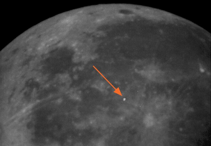
Figure 1. Lunar impact flash recorded in the framework of the ESA CARMEN project on 5 March 2022 at 19h23m16s UT, with a peak apparent magnitude of 5.
During the last decade we have performed important improvements in the systems employed to detect and analyze these flashes. Most of these advances involved the use of faster cameras with higher resolution working at different wavelengths. Here we focus on the systems employed by our team in the framework of ESA's CARMEN project, and also on two new systems deployed at the Calar Alto Observatory in Spain. One of these has been designed to perform observations in three wavelengths.
Contribution to the CARMEN project
Since 2021, and as a continuation of ESA's P3-NEO-I project, our team at IAA is member of a consortium of several astronomical observatories leaded by the companies Deimos Space and 6Roads. This consortium is conducting ESA's project “Consolidating Activities Regarding Moon, Earth and NEOs (CARMEN)”. and are one of the groups responsible for the work package (WP) dedicated to the detection and analysis of lunar impact flashes. One of the aims of this WP is the quantification of the flux of interplanetary matter that impacts our planet. For this purpose we have employed several telescopes located at two observatories in the south of Spain: La Sagra, and Sevilla. We are employing CMOS cameras with a maximum frame rate of 168 fps at full resolution (1920x1200 pixels). Figure 1 shows a sample lunar impact flash recorded with one of these devices in the framework of CARMEN.
New systems at Calar Alto
Our team has deployed a new telescope at the Calar Alto Observatory (Spain) and one of its goals is to observe lunar impact flashes. This instrument, which has an aperture of 60 cm, was initially intended to employ a system consisting of high-speed CMOS cameras (with a frame rate of 300 fps) to observe, simultaneously, at three different wavelengths (I, V and R). The telescope, which has been founded by the Spanish Ministry for Science and Innovation, is located within a dedicated 4-m automated dome. Figure 2 shows an image of this new instrument, which can be controlled remotely. However, it was finally decided to attach this 3-channel system to the 1,25m telescope located at that observatory. The 60-cm telescope would employ a single CMOS camera instead. Both systems are expected to enter operation in 2022, and would imply an important step for the analysis of the collision of meteoroids with the lunar ground.

Figure 2. The new 60 cm telescope deployed at the Calar Alto Observatory.
References
[1] Ortiz, J.L. et al., J., 1999. A search for meteoritic flashes on the Moon. Astron. Astrophys. 343, L57–L60.
[2] J.L. Ortiz, et al., 2000, Optical detection of meteoroidal impacts on the Moon. Nature 405, 921–923.
[3] Madiedo J. M., Ortiz J. L., Yanagisawa M., Aceituno J. and Aceituno F. (2019b). "Impact flashes of meteoroids on the Moon". Meteoroids: Sources of Meteors on Earth and Beyond, Ryabova G. O., Asher D. J., and Campbell-Brown M. D. (eds.), Cambridge, UK. Cambridge University Press, ISBN 9781108426718, 2019, p. 136-158
How to cite: Madiedo, J. M., Ortiz, J. L., and Morales, N.: Lunar impact flashes: observations in the framework of the ESA CARMEN project and development of new monitoring systems, Europlanet Science Congress 2022, Granada, Spain, 18–23 Sep 2022, EPSC2022-648, https://doi.org/10.5194/epsc2022-648, 2022.
The idea of commercially exploring small asteroids in the neighborhood of the Earth-Moon is not new. The interest in such minor objects is due to the fact that many of them have high concentration of metals and volatile (Elvis 2012, 2014), especially water. Exploratory missions could collect water from a near-Earth asteroid (NEA) and transfer it to a lunar orbit, where it could be used to produce fuel for rockets, to maintain human population in space systems, from which round-trip trajectories to other bodies in solar system would be less costly (Sercel 2017, Jedicke 2018, Steklov 2019). However, whether in terms of asteroid resource mining or to improve the scientific techniques for extraction, processing and storage of materials from low-gravity bodies, the cis-lunar space has been considered as a good location (Brophy et al. 2012, Mazanek et al. 2016, Jedicke et al 2018).
We numerically investigate the evolution and fate of ejecta produced by a supposed impact of an artificial projectile with a small asteroid or a boulder from it. In this scenario, we develop an idealized, realistic model to set up the initial state of the ejected particles, considering ejecta released at speeds at or below 1ms−1 from those stable Distant Retrograde Orbits previously determined by Pires & Winter (2020). The purpose of this study is to verify how much material might be delivered to the Earth or to the Moon, besides collision time relative to the position it was ejected in orbit. Our approach allows to gain insight into the dynamics of ejecta clouds generated by mining asteroids in the Earth-Moon vicinity. We verify how long do particles take to fall on each body. The time it took for particles to collide with massive bodies is an important measure when we deal with the realistic prediction of moving material as a result of impact cratering events or for human deflection. Regardless of the ejection speed, particles that fall on the Earth or on the Moon, completed they journey in less than 5 years after being launched into space, or take more than 500 years to have about 1% of them colliding with both bodies. Between 5 and 500 years, the number of collisions is practically null. Most part of the low-speed regolith are lost to space. They escape the system as time advances. The process of loss of ejecta is stronger at the beginning of the numerical simulations and goes to approximately 10 years. There were a sample of ejected particles that remain bounded to the Earth-Moon system during the whole time of numerical simulations (10 K-years). Our methodology is based on several numerical simulations of ejecta using an N-Body code to calculate their evolution accounting its gravity interaction with the massive bodies: the Earth and the Moon, beyond the Sun. Our numerical simulations inputs covers a small range of low-speed ejecta as a result of impact cratering events. We have come up with results that have shown impact ejecta moving at speeds of order millimeter to meters-per-second reach the Earth or the Moon very quickly (less than 5 years) for a given range of initial conditions and assumptions. We will present our main results in terms of histograms and orbital evolution.
How to cite: Pires dos Santos, P. M., Winter, O. C., and Amarante Luiz, A.: Analysis of the evolution of particles ejected from Lunar Distant Retrograde Orbits, Europlanet Science Congress 2022, Granada, Spain, 18–23 Sep 2022, EPSC2022-718, https://doi.org/10.5194/epsc2022-718, 2022.
Polycyclic aromatic hydrocarbons (PAH) are ubiquitous organic molecules populating the interstellar medium of galaxies and they are the major responsible of interstellar infrared spectral features (e.g., Allamandola et al. 1989, Tielens 2008). PAH are also found as constituents in carbonaceous chondrites (e.g., Kalpana et al. 2021). Similarly to silicate dust, carbon-rich micrometric and submicrometric aggregates occur in different astrophysical environments where they are subjected to several weathering processes such as impact shock events and grain-grain collisions. These processes change the chemistry and structure of the original materials giving rise to new chemical species which contribute to the chemical richness of the cosmic environment (e.g., Murri et al. 2022; Mimura et al. 1995). The study of the chemical and structural evolution of aggregates of PAH subjected to extreme conditions is relevant for examine in depth the origin of the densest phases of carbon (e.g., pre-solar grains) as that of prebiotic building blocks of life (Giese et al. 2022). For this purpose, a lot of effort has been made by the whole scientific community for reproducing in laboratory the planetary conditions which trigger the processing of cosmic dust. In this framework, high-energy pulsed lasers represent consolidated tools for reproducing the high energy-density conditions similar to those occurring in shock events in the interstellar medium as a consequence of supernova explosions. Liquid-phase pulsed laser ablation (LP-PLA) is a technique in which high-energy laser pulses are focused on the surface of a solid target immersed in a liquid to induce ablation of material as a result of the ignition of a plasma plume, and recondensation of the ablated material in the surrounding liquid in the form of suspended nanoparticles. The presence of the liquid augments to a great extent the pressure achieved at the solid/liquid interface and allows the onset of cooling rates of the order of 105 K s-1, likewise to what occurs in circumstellar environments. Using this technique, nanodiamonds are commonly produced from graphite targets in water or organic liquids (e.g., Amans et al., 2017).
In this paper we report the results of the high-energy laser processing of a pure nano-phase of rubrene (5,6,11,12-tetraphenyltetracene), a PAH constituted by a backbone of four fused benzene rings (tetracene) bonded to four phenyl rings (Figure 1). The choice of rubrene is motivated by the possibility to obtain commercially available batches of purity higher than 99.9%, its ability to organize in a high-symmetry molecular crystalline phase, and the in-depth knowledge of the photophysical and photochemical properties of both the isolated molecule and molecular aggregates. All these characteristics make rubrene an ideal model system to study the evolution of PAH in response to high-energy processing. We performed LP-PLA of rubrene nano-phases dispersed in water (i) to simulate space weathering in a water environment (e.g., hydrous or volatile-rich bodies) and (ii) to study its chemical and structural evolution. The laser processing of the water suspension was monitored by optical spectroscopy (absorption and luminescence) and high-resolution transmission electron microscopy and diffraction analyses.
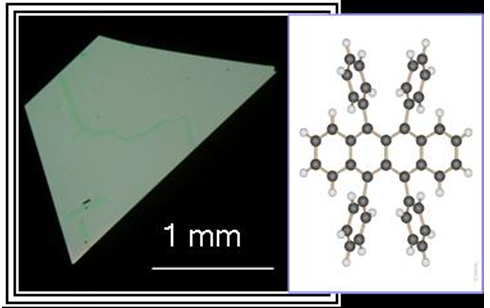
Figure 1. Molecular structure of rubrene (C42H28) and optical micrograph collected with cross polarizers on a thin orthorhombic single crystal or rubrene.
We observed that laser processing brings about a progressive suppression of the absorption band in the visible range of the pristine rubrene nanocrystals, with increment of the signal in the UV range, indicating their transformation into a different phases. The structural and chemical features of these new phases are inferred by high-resolution transmission electron microscopy and analysis and compared with known carbon-rich phases populating the interstellar medium.
Acknowledgments
Funding of the University of Milano – Bicocca through grant 2021-ATEQC-0054 is acknowledged. We are grateful for the support of Giancarlo Capitani for electron microscopy analyses.
References
Allamandola et al. (1989), The Astrophysical Journal Supplement Series 71, 733−775.
Amans et al. (2017), Journal of Colloid and Interface Science 489, 114–125.
Giese et al. (2022), ACS Earth Space Chemistry 6, 468−481.
Kalpana et al. (2021), Planetary and Space Science 198, 105177.
Mimura et al. (1995), Geochimica et Cosmochimica Acta 59, 579−591.
Murri et al. (2022), ACS Earth and Space Chemistry 6, 197−206.
Tielens (2008), Annu. Rev. Astron. Astrophys. 46, 289–337.
How to cite: Campione, M. and Murri, M.: Laboratory simulation of space weathering of nano-aggregates of polycyclic aromatic hydrocarbons dispersed in the water environment, Europlanet Science Congress 2022, Granada, Spain, 18–23 Sep 2022, EPSC2022-801, https://doi.org/10.5194/epsc2022-801, 2022.
Introduction: The dating of geological surfaces on the Moon is crucial for understanding its geological history and evolution. The measurement of Crater Size-Frequency Distributions (CSFDs) can be used for determining relative and absolute ages of surfaces. Older surfaces reflect more and larger craters than younger geological units [1-4]. To determine the relative surface ages, a production function (PF) is constructed to which the CSFD is fitted. One frequently used PF was empirically-derived by measuring craters on reference surfaces using Apollo era data (Neukum, 1983 [1]), which was revised in 2001 [5], and is valid for crater diameters of 10 m - 300 km and 10 m - 100 km, respectively. With increased image resolution of more recent missions [e.g., 6], it has been possible to measure CSFDs for crater diameters down to a few meters. Therefore, it would be beneficial to be able to extend the PF to smaller crater diameters, which would allow the determination of relative and absolute ages for young/small geological units.
A crucial influence on small craters formed in the strength regime are target properties, which has been investigated in several studies [e.g., 7, 8, 9]. Therefore, we aim to perform the crater counts exclusively on continuous ejecta blankets. Secondary craters [e.g., 10-12] influence the CSFD as well and can contaminate the count area, causing a steeper CSFD-slope [e.g., 10, 13, 14]. To avoid this effect and obtain the cleanest PF possible, we selected ejecta areas derived from young Copernican-aged craters. This minimizes the number of field secondary craters on the ejecta and also avoides major degradation of the small craters [15, 16]. However, the identification of self-secondary craters remains problematic, since they occur irregularly distributed on the ejecta blankets and often have morphologies similar to primary craters [e.g., 12, 13].
Method: We used Lunar Reconnaissance Orbiter Narrow Angle Camera (NAC) images [6] including M180509194LE, M1122929850LE and M103831840LE/RE at Giordano Bruno (GB), M1107052575RE and M1112971104RE at Moore F, M129187331LE/RE at North Ray (NR), M119754107RE at South Ray (SR) and M114064206LE at Cone. The resolutions vary between 1.6 m/px and 0.5 m/px, the incidence angles are from 54° to 78°. The CSFDs were measured in ArcGIS with the CraterTools add-in of [18] and displayed in CraterStats with pseudo-log binning [19].
Two areas were investigated at Cone, three at GB, Moore F and SR, respectively. Four areas were investigated by [17] at NR. The selected counting areas are all on the ejecta blakets of the named craters.
Results: Similar to [17] we combined the statistics from the separate count areas into one file and display these CSFDs in a cumulative plot in Figure 1.

Figure 1: Display of the combined CSFDs at GB (green), Moore F (blue), NR (violet), SR (red) and Cone (orange), respectively. The vertical lines of individual data points represent the error bars.
The comparison between the individual CSFD-slopes at GB, Moore F, NR, SR and Cone generally show slightly steeper slopes than the nominal -3 slope of [1] for crater diameters between 10 m and 23 m (in our case 20 m, see Table 1).

Table 1: Display of the considered crater diameter range and the respective CSFD-slopes.
Discussion: We found that the CSFD-slopes on the ejecta blakets of the investigated craters show a tendency regarding the crater diameter. Considering only diameters ≤10 m the slope is marginally shallower than Neukum’s [1] -3 slope, except at GB, which might be explained through secondary cratering. This trend was also observed by [15] (and references therein) and [20] who investigated NR, Cone, Copernicus and Tycho. This might suggest that CSFDs of young Copernican craters have actually a slightly shallower slope at smaller crater diameters. Another possible explanation is the faster degradation of smaller craters [e.g., 21]. Further effects might be the coverage of ejecta material of nearby craters; NR (52.3 Ma [20]), might be influenced by the ejecta of SR (2 Ma [22]), SR by Baby Ray. Moreover, larger craters in two areas at NR and Cone probably penetrated through the ejecta blanket, which can lead to mixed target propertie effects.
Further investigations are required to quantify the effects of secondary cratering, target properties, crater degradation or impactor flux on the determination of our CSFDs. Additional investigation is necessary to determine at which crater diameter the slope becomes shallower or if a transition zone is present.
Acknowledgments: This Project is funded by the Deutsche Forschungsgemeinschaft (DFG, German Research Foundation) – Project-ID 263649064 – TRR 170.
References: [1] Neukum (1983), NASA TM-77558. [2] Öpik (1960), RAS 120(5), 404-41. [3] Shoemaker et al. (1970), Science, 167 (3918), 452-455. [4] Baldwin (1971), Icarus, 14, 36-52. [5] Neukum et al. (2001), Space Sci. Rev., 96, 55. [6] Robinson et al. (2010), Space Sci. Rev. 150, 81-124. [7] van der Bogert et al. (2010), LPSC 41, #2165. [8] Wünnemann et al. (2011), Proceedings of the 11th hypervelocity impact symposium., Vol. 20. [9] van der Bogert et al. (2017), Icarus, 298, 49-63. [10] McEwen and Bierhaus (2006), Annu. Rev. Earth Planet. Sci. 34, 535-567. [11] Xiao and Strom (2012), Icarus 220, 254. [12] Zanetti et al. (2017), Icarus 298, 64-77. [13] Plescia et al. (2010), LPSC 41, #2038. [14] Plescia and Robinson (2011), LPSC 42, #1839. [15] Moore et al. (1980), Moon and Planets, 23, 231-252. [16] Fassett and Thomson. Journal of Geophysical Research: Planets 119.10, 2255-2271. [17] Hiesinger et al. (2012), JGR 117, E00H10. [18] Kneissl et al. (2011), PSS 59, 1243-1254. [19] Michael et al. (2016), Icarus 277, 279-285. [20] Williams et al. (2014), Icarus 235, 23-36. [21] Mahanti et al. (2018), Icarus, 299, 475-501. [22] Stöffler and Ryder (2001), Space Sci. Rev., 96, 9-54.
How to cite: Oetting, A., Hiesinger, H., and van der Bogert, C.: Refinement of the Lunar Production Function - The CSFD-Slope of Small Crater Diameters on Ejecta Blankets, Europlanet Science Congress 2022, Granada, Spain, 18–23 Sep 2022, EPSC2022-828, https://doi.org/10.5194/epsc2022-828, 2022.
1. Introduction
Asteroid impacts, ranging from small-scale cratering events to catastrophic disruption, have played a crucial role in the formation and evolution of asteroids (Jutzi et al., 2015). Thanks to the increasing performance of computers, shock-physics numerical codes have become commonly used in the field of hypervelocity impacts, to extrapolate experimental results and help us be better prepared for space missions devoted to asteroid deflection using the kinetic impactor techniques, such as the NASA DART (Rivkin et al. 2020) and ESA Hera missions (Michel et al. 2022), and evaluate the outcomes.
Past numerical studies showed us that it is possible to divide the asteroid impact process into two stages that occur at very different time scales, the early stage of fragmentation of the asteroid and the late stage of gravitational reaccumulation of the fragments (e.g, Michel et al. 2001). For the early stage, various numerical methods have been developed to solve this short but extreme physical process, such as the Smooth Particle Hydrodynamics (SPH) technique used in codes like the Bern SPH and grid techniques used in codes like CTH or iSALE. Each method has its unique advantages, but they share a common challenge that the contact and the boundary condition are not well handled (El Mir et al., 2019).
In this study, we exploit the Material Point Method (MPM) framework, an extension of the particle-in-cell method, to simulate the early stage of impact in order to offer a new approach and solutions to the above problems.
2. Methods
MPM is a meshfree method, characterizing the material domain by a group of points. These Lagrangian material points carry all state variables. Meanwhile, a predefined regular background grid is used. In each timestep, material information is mapped to grid nodes, to solve the momentum equations, and material points deform with the grid. Then the information is mapped back to the points to update their positions and velocities, discard the deformed grid, and reset a new one to calculate the next timestep (Zhang et al., 2013). MPM framework combines the advantage of both Lagrangian description and Eulerian description, which not only avoids the undesirable mesh tangling caused by large deformations, but also eliminates the difficulties in solving contact and boundary conditions.
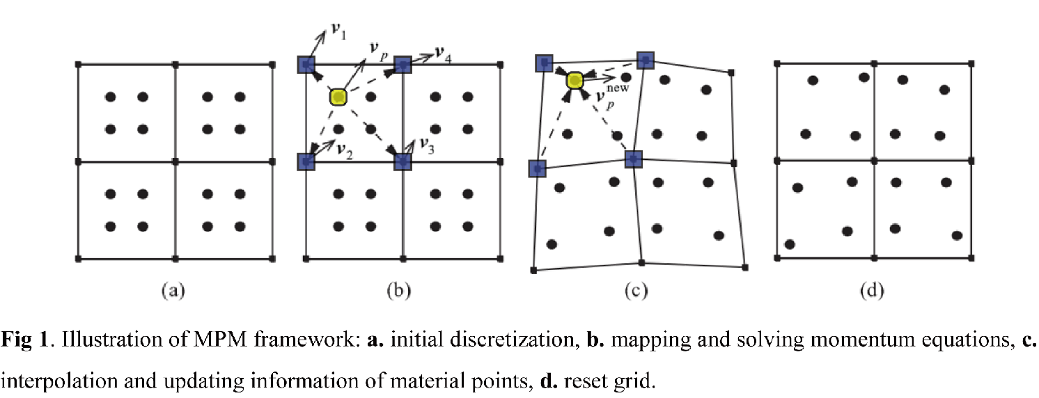
As such, MPM is well used in simulating impacts, explosions, and metal forming of on-earth situation (Zhang et al., 2013). So far, it has not been commonly used to model hypervelocity impacts on asteroids (El Mir et al., 2019). Hence, we start with building material models that are applicable to asteroids made of porous and brittle materials.
The material models include Drucker-Prager strength model that describes cohesion and pressure-dependent strength effect. We also use the Tillotson equation of state for basalt coupled with the P-alpha model which accounts for porosity, and as stress-based failure criterion consistent with Weibull distribution. The framework is thus similar to that used by other studies using the SPH numerical method (Raducan and Jutzi, 2021). Our MPM model is then validated by comparing with laboratory impact experiments and the simulations using the SPH method.
3. Results
We compare our simulations with SPH simulations (Benz & Asphaug, 1994) and the impact experiments (Nakamura et al., 1991) on non-porous basalt sphere used to validate them. Our result shows that our material model under the MPM framework can successfully characterize the shell-like propagation of the failure zone (Fig 2.c2). However, a concentration of stresses reflected back from the boundary subsequently occurres, resulting in a severe secondary failure in the nuclear region. (Fig 2.c3) This stress concentration may cause by the unsmooth discrete boundary and the lack of energy dissipation. The analysis of large fragments reveals this problem too: although with a similar mass distribution, the velocity of the largest fragment in MPM simulation is significantly higher (Fig 3.a). Apart from that, the simulation results are otherwise in good agreement with the previous studies, especially the shape of the largest fragment of MPM simulation (Fig 3.b) versus a recent experiment (Fig 3.c). Noting the usual spreading in experimental outcomes using same conditions, the MPM method can thus be considered valid.
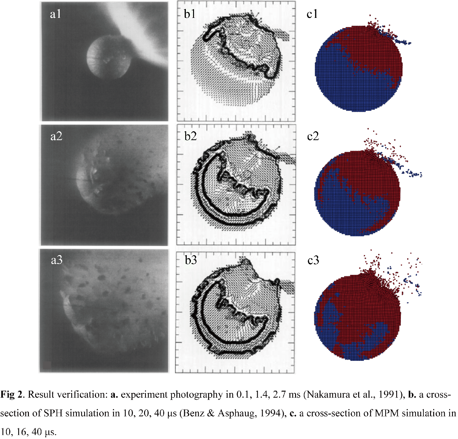
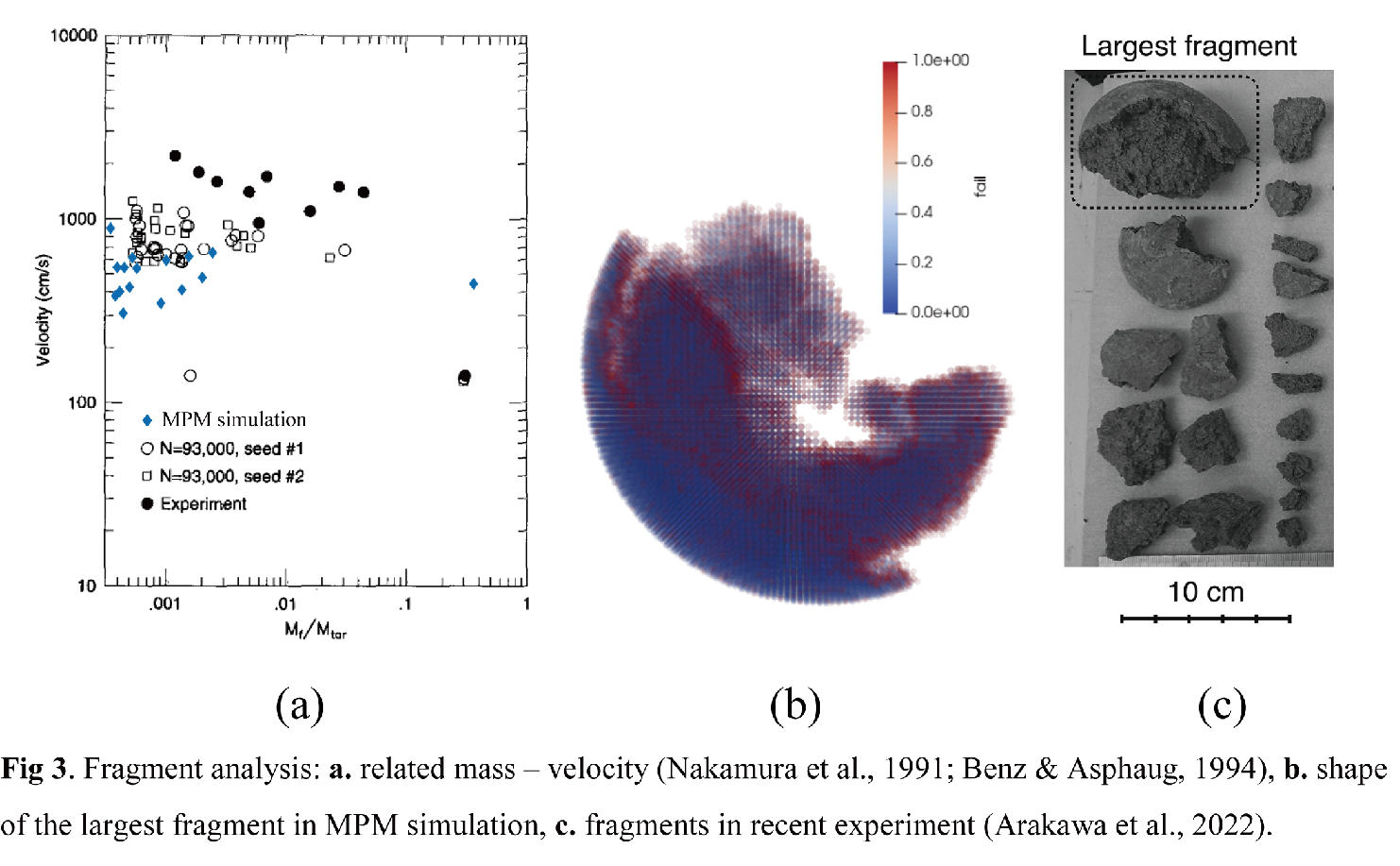
Further research will be centered on verifying the P-alpha model and the correct treatment of porosity (Jutzi et al., 2009).
4. Conclusion and Discussion
The MPM framework can complement of other shock-physics code to balance the accuracy and efficiency of calculation. Furthermore, the mentioned features of solving contact and boundary conditions with MPM broadens the application of the simulation algorithm in the hypervelocity impact stage, and may make it easier than SPH models to combine with the Soft-Sphere Discrete Element Method (SSDEM) code (Fig 4) to simulate the two-stage impact process (SPH-SSDEM method refers Zhang et al., 2021).
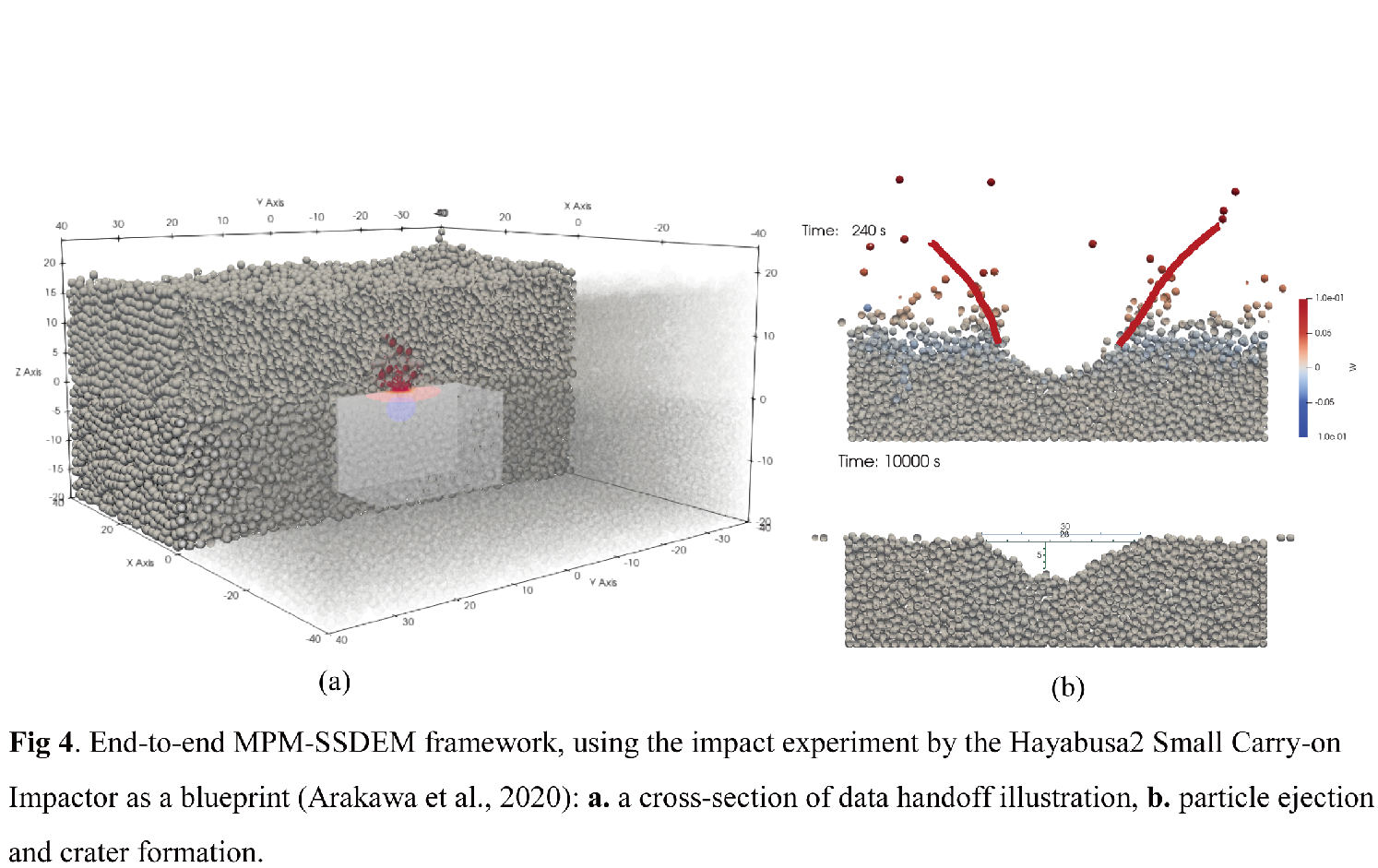
All these studies will offer a glimpse into the active processes from the early formation of the solar system to the current epoch, and contribute to planetary defense.
Acknowledgements:
We acknowledge support from the Université Côte d’Azur. X.Y. acknowledges support from Tsinghua University, funding from the Chinese Scholarship Council, and the National Natural Science Foundation of China (No. 11872223). P.M. acknowledges funding from CNES, from the European Union’s Horizon 2020 research and innovation program under grant agreement No. 870377 (project NEO-MAPP) and from the CNRS through the MITI interdisciplinary programs.
References:
Arakawa, M. et al. (2020) Science, 368, 67–71.
Arakawa, M. et al. (2022) Icarus, 373, 114777.
Benz, W., & Asphaug, E. (1994) Icarus, 107(1), 98–116.
El Mir, C. et al. (2019) Icarus, 321, 1013–1025.
Raducan, S.D. & Jutzi, M. (2021) 52nd LPSC, #1900.
Jutzi, M. et al. (2009) Icarus, 201(2), 802–813.
Jutzi, M. et al. (2015) In: Asteroids IV (Michel P. et al., eds.) 679–699.
Michel et al. (2001) Science, 294, 1696-1700.
Michel et al. (2022) Planetary Science Journal, accepted.
Nakamura, A., & Fujiwara, A. (1991). Icarus, 92, 132–146.
Rivkin, A. et al. (2020) Planetary Science Journal, 2, 173.
Zhang, X. et al. (2013) Beijing: Tsinghua University Press.
Zhang, Y. et al. (2021) 52nd LPSC, #1974.
How to cite: Yan, X., Liu, Y., Zhang, Y., Michel, P., and Li, J.: Hypervelocity impact simulation on asteroids with MPM framework, Europlanet Science Congress 2022, Granada, Spain, 18–23 Sep 2022, EPSC2022-1064, https://doi.org/10.5194/epsc2022-1064, 2022.
Introduction
A lunar impact flash (LIF) is a rapid burst of light caused by a hypervelocity impactor hitting the moon, releasing a fraction of its energy as light. They are observable though moderately sized (0.4m) telescopes, and are therefore observable by both amateur and professional astronomers.
LIF observations are typically performed in visible or NIR, and can only take place when the lunar phase is between 10-50%, during local night, and are only observable against the lunar night-side; the most commonly observed LIFs are faint, approximately MagI = 9, MagR = 10 [1], making them indistinguishable against the illuminated lunar background. This limits potential observations of LIFs to ~30h per month on average, with weather limiting this further.
In order to increase the average number of observable hours that LIF observations can be made, and thereby increase the number of observed LIFs, we have developed new techniques to perform LIF observations at all local times, and all lunar illuminations. This technique theoretically only requires clear weather and a visible moon.
Theory
LIFs have been shown to behave as black bodies, releasing energy according to Planck's law [2]. The temperature of LIFs observed by NELIOTA is between 1300-5800 k, with average temperature, Tavg = 2800k [3]. This average has peak wavelength of λpeak = 1.035 μm. The illuminated portion of the lunar surface is reflecting light from the sun (T = 5778 k, λpeak = 0.5 μm). In R-band and I-band, the ratio of energy radiated by the sun is greater by a factor of 57 in R-band, and 28 in I-band. My observing in wavelengths closer to the λpeak of the flash, we can improve this ratio greatly.
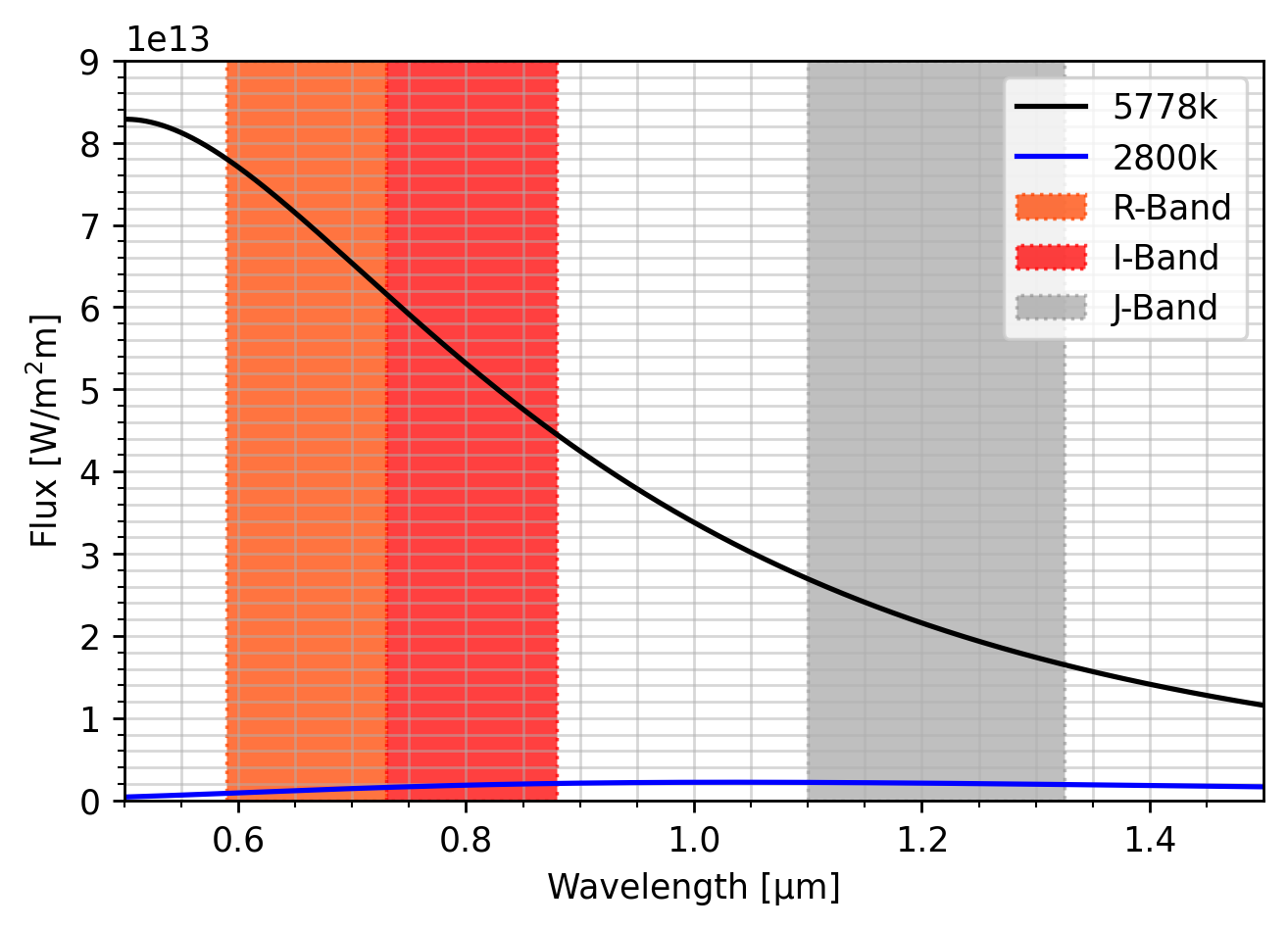
Figure 1:The Planck curve for the sun (5778k) and the average LIF (2750k), R, I, and J-band regions are highlighted in orange, red, and grey respectively.
As illustrated in Fig. 1, by observing in J-band the irradiance of the sun is lowered, being only 10 times greater than the 2800 k LIF. This effective dimming of the background leads to an increase in the signal-to-noise ratio (S/N) of the LIF against the sun-illuminated background.
The S/N ratio is a measure of how detectable a signal is above the background, and can be defined as:
S/N = S" / (σ × √Apix)
Where S" is the total count of the signal, σB is the standard deviation of the background, and Apix is the area of the background measurement. A S/N ratio above ≈10 is generally required for a signal to be considered detectable.
Observations
Observations were performed on 2022-02-23 from the Observatoire de la Côte d'Azur, using a 0.5 m diameter, 2 m focal length telescope with Ninox 640 II camera and J-band filter attached. For the first set of observations, high gain mode was used, for the second set of observations low gain mode was used. A 30 μm exposure time was used for both sets of observations.
The star HD137463 was observed, which has MagJ = 5.423, obtained by Simbad [4] Observations began during the night, and continued until after sunrise in order to measure the brightness of the sky during daytime.
By performing A-B subtraction to remove the dark current and background of the observed frames, as shown in Fig. 2, a pixel count for the clean star signal, S", can be obtained. As it is constant, an average for the star signal can be used as ground truth in order to calculate the S/N ratio for the daytime sky brightness, as well as the illuminated lunar surface.

Figure 2: The A-B subtraction of two observations of HD137463. The subtraction removes any dark current or background to leave only a clean positive and negative signal.
Results
The S/N ratio for the a MagJ = 5.423 star are shown in Fig. 3. A sharp decrease in S/N ratio is observed as air-glow begins around solar altitude = -5. The S/N continues to decrease, slowly levelling off around S/N = 15 as the sun reaches solar altitude = 5. This puts the magJ = 5.423 star well above the detectable threshold, and would correspond to a MagR = 6.7 LIF.

Figure 3: Left: The S/N ratio in high gain mode, of HD137463 against the sky background between solar altitudes -10 & -1. Right: The S/N ratio in low gain mode, of HD137463 against the sky background between solar altitudes -1 & -5.
By taking measurements of the lunar background brightness, we can verify the S/N ratio we would expect from these LIF when observed on the lunar surface. Table 1 contains the results from count-averaged observations of the background, and the S/N of the MagJ star if observed against the background, emulating a flash. Again, even against the illuminated bright limb, the S/N ratio is above the detectable threshold, and shows that with this system, we would be able to detect LIFs of MagJ ≥ 5.423, with the possibility of even fainter magnitudes under more favourable conditions.
Table 1: The S/N ratio of the reference star used against different regions on the lunar surface, from darkest to brightest.
| Region | S/N |
| Lunar Night Side | 147 |
| Terminator | 42 |
| Lunar Day Side | 21 |
| Lunar Bright Limb | 19 |
References
[1] Liakos et al (2019) A&A, 633, 29 pp.
[2] Eichhorn (1975) P&SS, 23, 11, 1519-1525
[3] Avdellidou & Vaubaillon (2019) MNRAS, 484, 5212-5222
[4] Wegner et al (2000) A&A, 143, p.9-22
How to cite: Sheward, D., Delbo, M., Avdellidou, C., Cook, A., and Lognonne, P.: J-Band Measurements for All-Hours Lunar Impact Flash Observations, Europlanet Science Congress 2022, Granada, Spain, 18–23 Sep 2022, EPSC2022-1077, https://doi.org/10.5194/epsc2022-1077, 2022.
TP15 | Astrobiology
To be sustainable, a settlement on Mars should be as independent of Earth as possible in terms of material resources. This independence may be reached with the help of biological systems: those could perform a wide range of functions with a low impact on the surroundings. However, biological systems would best rely on resources available on Mars – as recycling alone would mean that the amounts of available resources decrease over time – and most organisms cannot utilize raw Martian resources directly.
A solution has been proposed which lies in using diazotrophic, rock-weathering cyanobacteria. Their physiology is such that they could, it seems, be fed with materials available on site: water mined from the ground or atmosphere; carbon and nitrogen sourced from the atmosphere; and the local regolith, from which it has been argued that they could extract the other necessary nutrients. The cultured cyanobacteria could then produce various consumables directly, such as dioxygen and dietary supplements but also support the growth of secondary producers (plants or microorganisms) which could, in turn, generate a wide range of critical consumables.
Various proofs-of-concept have been reported in the literature and evidence accumulates that some cyanobacteria could, indeed, be fed from Martian resources and provide feedstock for other organisms of biotechnological interest. But whether a system works at all is not sufficient to decide whether it should be integrated into mission plans: its cost-efficiency must be determined and compared to potential alternatives.
Among the factors that will determine this cost-efficiency is the fitness of cyanobacteria under (i) hypobaria (low pressures), and as a result low partial pressures of dinitrogen; and (ii) a dependence on regolith for all nutrients not provided as gases, which would also lead to high concentrations of highly oxidizing compounds (chiefly, perchlorates) in the extracellular medium. Another key element is the design of specific cultivation hardware.
In this presentation, we will present the wet-lab and in-silico work performed at the ZARM’s Laboratory of Applied Space Microbiology to study those factors and thereby assess, and improve, the efficiency of cyanobacterium-based, biological ISRU on Mars.
How to cite: Verseux, C. and Ramalho, T.: On the cost-efficiency of cyanobacterium-based, biological ISRU on Mars, Europlanet Science Congress 2022, Granada, Spain, 18–23 Sep 2022, EPSC2022-57, https://doi.org/10.5194/epsc2022-57, 2022.
Introduction
The survivability of bacteria in planetary impacts has previously been investigated using a two-stage Light Gas Gun (as seen in Figure 1). During these experiments, projectiles were doped with bacteria (Rhodococcus erythropolis) and fired at hypervelocity into rock [1,2], metal [2], water-ice [3,4] and agar [4,5] targets. These experiments were designed to investigate the feasibility of the panspermia theory, which details how indigenous life forms may be spread beyond their host body via the ejecta created by hypervelocity impacts and go on to seed neighbouring bodies. These studies showed that bacteria do survive hypervelocity impact; however, the methods do not accurately quantify the survival rate on the target compared to the initial cell load on the projectile, nor do they quantify or characterise any sub-lethal effects.

Figure 1: The Light Gas Gun impact facility at the University of Kent.
Creating A Successful Target
Attempts have been made to develop new methods that give greater quantitative insights into both survival and sub-lethal effects of hypervelocity impacts. As well as investigating the survival rate of the bacterial population, we are looking at whether the transient extremes of pressure which occur as a result of hypervelocity impact modulate phenotypic change amongst the surviving bacteria, and thus could be a factor in the evolution of life.
The bacteria (in this case Escherichia coli) in our experiments have been placed inside the target instead of the projectile. This decision was made in order to remove the potential issues of the loss or death of cells as a result of the acceleration of the projectile. Several different target designs were trialled, largely involving the use of agar as a medium for housing the bacteria. These attempts led to a set of criteria being defined for a successful target, including efficient propagation of the shock wave through the sample to ensure that the bacteria are experiencing the intended conditions, and clean recovery of the majority of the sample with little or no contaminants.
The Liquid Target Setup
Following much experimentation, a liquid target setup was created, as seen in Figure 2. A 50 ml liquid sample containing the bacteria is housed inside a thin polythene bag and placed inside a steel tube, which upon impact collects the liquid and allows for ease of recovery and analysis. The impacted plastic bag produces a large amount of debris within the collected sample, which interferes with some of the optical data gathered during post-impact analysis of the bacteria. Also, there is concern that the entirety of the sample is not experiencing the full force of the impact. To address these issues, we are designing a secondary tube with a much smaller diameter which can be inserted and secured inside the primary steel tube; this should mean that more of the sample volume will experience higher shock pressures in the range of several GPa, which can be verified by simulating the impacts using Autodyn modelling. To replace the polythene bag, and thus attempt to minimise the quantity of debris entering the system, the liquid sample will be sealed directly inside the secondary tube with an extremely thin foil.
Impacts have been completed across the velocity range of 1-5 km/s using this setup. The following analysis methods have been applied to the recovered samples post-impact:
- OD600 (optical density) recordings to understand changes in whole cell numbers by measuring the number of particles within a given sample
- Protein assays to understand the amount of physical damage or lysis to the cells
- Growth on agar plates to understand how the viability of the population has changed via the counting of colony forming units (CFUs)
- Oxygen electrode analysis to see if the metabolic pathways of the cells have been affected by measuring cellular respiration in the presence of glucose
So far, no significant changes to the survival rate or the phenotype of the population have been observed following these impacts using the analysis methods described.

Figure 2: The liquid target setup within the target chamber of the Light Gas Gun.
Influence of Exposure Time to Impact Conditions
The results from the liquid target impacts have raised the question of whether the extremely short duration of the shock pressure is insufficient to lead to any meaningful change in the bacterial population. To investigate this, E. coli samples prepared in the same manner as for the impacts are instead placed inside a sonicator, where the sound waves generate pressures within the sample of around 200 MPa, compared to the impact shock pressures of several GPa created in the Light Gas Gun. The sonication exposure times were varied, using 4 bursts of 0, 5, 10, 30 and 60 seconds, compared to the milliseconds or less that the peak shock pressures are applied to the sample in the Light Gas Gun.
A steady decline of surviving bacteria and a significant increase in cell lysis was observed as the exposure time was increased, supporting the idea that time is the key factor in generating populational changes. At burst exposure times of 30 seconds or more, an unusual phenotype emerges following growth of the sonicated samples in the form of a new colony type displaying a concentric ring pattern of growth, as shown in Figure 3. This is currently being investigated further with repeat experiments, antibiotic testing and 16S rRNA sequencing to confirm that this is indeed a change in phenotype and not a result of a separate factor such as contamination.

Figure 3: An agar plate spread with a sample of E. coli cells following 4 30-second bursts of sonication.
References
[1] Burchell et al. (2000) In Gilmour I., Koeberl C. (eds) Impacts and the Early Earth. Lecture Notes in Earth Sciences, vol 91.
[2] Burchell et al. (2001) Adv. Space. Res. 28(4), 707-712.
[3] Burchell et al. (2003) Origins of Life and Evolution of the Biosphere 33, 53-74 (2003).
[4] Burchell et al. (2004) Mon. Not. R. Astron. Soc. 352, 1273-1278 (2004).
[5] Burchell et al. (2001) Icarus 154, 545-547 (2001).
How to cite: Wilkinson, R., Wozniakiewicz, P., and Robinson, G.: Exploration of Methodologies to Investigate Bacterial Survival in Planetary Impacts, Europlanet Science Congress 2022, Granada, Spain, 18–23 Sep 2022, EPSC2022-121, https://doi.org/10.5194/epsc2022-121, 2022.
Exploring the limits of life is one of the objectives for better understanding how organisms have arisen on Earth, how they tolerate extreme conditions and how they might survive on other planets or moons. These investigations could help with understanding which Earth microorganisms could survive on other celestial bodies, such as the icy Moons: Europa (Jupiter) and Enceladus (Saturn). Furthermore, it might help with indicating how life could have developed on Earth or on the icy Moons of the Solar system. This project focuses on the insights from prokaryotic, eukaryotic and archaea organisms which can tolerate the simulated subsurface ocean environment of Europa and Enceladus. The moons have been speculated to have subsurface oceans which are heated by tidal movements or hydrothermal vents. These combined factors could create an environment suitable for life. Furthermore, the mechanism of radiation, desiccation and temperature survival could help us understand whether the organisms could survive a hitchhike on spacecraft surfaces travelling to the moons. During space exploration it is essential to avoid the contamination of planets and moons of astrobiological interest by microorganisms from Earth.
The projects’ main question is: What are the boundaries of tolerance for cold-adapted halophilic microorganisms as determined by simulated space conditions? Furthermore, we also want to investigate the survival to simulated icy moon conditions. At this stage of the project two organisms have been investigated, the bacterium Planococcus halocryophilus and the yeast Rhodotorula frigidalcoholis. Our aim is to use one organism from each domain of life: prokaryote, eukaryote and archaea. Preliminary results have shown a fair survival of R. frigidalcoholis but not of P. halocryophilus to some simulated space conditions. In order to find better suited bacterial and archaea candidates we will be investigating cold adapted microorganisms from astrobiologically relevant sites. Examples include the Shaban deep, a brine sediment in the Northern Red sea, permafrost core, Antarctic soil samples, glacier ice and arctic sea-ice cores. The bacteria we have selected are the following: Paenisporosarcina antarctica, Psychromonas boydii, Cryobacterium flavum, Virgibacillus arcticus and Chromohalobacter saracensis. The archaea are: Halorubrum luteum and Halorhabdus tiamatea.
The results we processed have shown that R. frigidalcoholis is more tolerant than P. halocryophilus to monochromatic UV-C (254 nm) and polychromatic UV (200-400 nm) as well as X-ray. When exposed to desiccating conditions, at different temperatures, the difference between the two organisms is not so noticeable. The results which we present here have been developed from the microorganisms grown under minimal media conditions, supplemented with a sole carbon source (L-Glutamic acid for R. frigidalcoholis and D-Alanine for P. halocryophilus). The decision to use minimal media and single carbon sources, not as common as glucose, was in support of simulating stress growth conditions to an extent similar to the ones on Europa and Enceladus. Planetary bodies where some simple organics have been detected in low concentrations.
Despite the two organisms being isolated from similar environments, R. frigidalcoholis from ice cemented permafrost in University valley (Antarctic) and P. halocryophilus from permafrost active-layer soil in the Canadian High Arctic, they have great differences in their tolerance to extreme conditions. Tested conditions include desiccation survival at: room temperature, -20 and -80°C under oxic and anoxic conditions. Additionally, we can describe a fair survival of R. frigidalcoholis to weekly freeze-thaw conditions from -80°C to 25°C respectively.
Being two organisms isolated from arctic-like environments, our hypothesis supported a great tolerance to freeze and thaw conditions. The reduction in relative survival of R. frigidalcoholis to an order of magnitude of 10-2, supports our hypothesis. Of importance to note for this experiment are the -80°C freezing conditions. In the literature similar tests are conducted at higher temperatures (-40 and -10°C).
The preliminary results exposing R. frigidalcoholis and P. halocryophilus to harsh growth conditions are useful for initial expectations to survival in environments similar to the ones on Europa or Enceladus. For continuing and future research, this project could be of particular interest for defining a protocol for microbial exposure to simulated extreme environmental conditions. As well as to support the development of suitable planetary protection measures. The following graphs show the results of the described experiments. The figures include in formation on the relative survival of organisms and the F10 values for each condition. The F10 values have been included to represent the dose to which there is 10% survival to the exposed condition.
UV-C Irradiation:
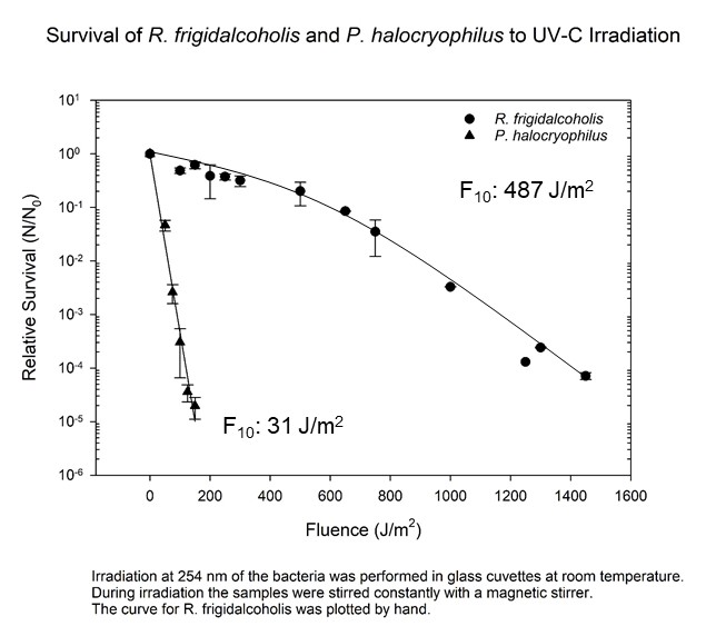
Polychromatic UV Irradiation:
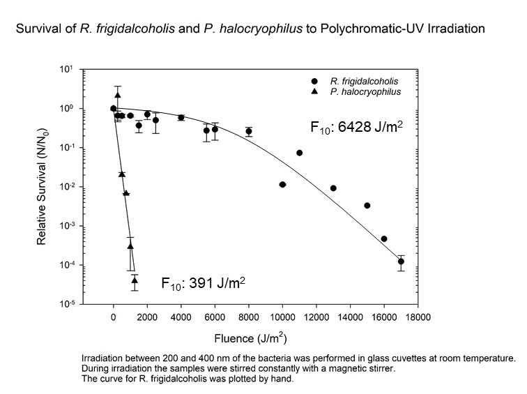
X-ray Irradiation:
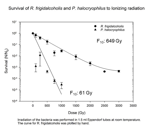
How to cite: Zaccaria, T., Rettberg, P., Beblo-Vranesevic, K., De Jonge, M., and Netea, M.: Investigation of the physiological response of cold-adapted microorganisms to extreme environmental stress factors., Europlanet Science Congress 2022, Granada, Spain, 18–23 Sep 2022, EPSC2022-206, https://doi.org/10.5194/epsc2022-206, 2022.
Abstract
What is life and how could it originate? This question lies at the heart of understanding the cell as the smallest living unit. Although we are witnessing a golden age of life sciences, we are ironically still far from giving a convincing answer to this question. With the aim to examines potential source of energy available to protocells on early Earth and/or elsewhere and mechanisms by which the energy could be used to drive polymer synthesis, experiments aimed at revealing the ability of meteorites and some terrestrial rocks to perform catalytic reactions operative in present-day life have been performed.
1. Indroduction
The aim of this work is to present and discuss results of recent and ongoing wet-lab experiments supporting Multiple Root Genesis Hypothesis (MuGeRo) already proposed elsewhere [1] seeking approaches surrounding the mysterious primeval steps of life emergence on Earth or on planets around distant stars beyond our Galaxy. This is an additional hypothesis to that microbial or early forms of life were already present in our solar system at the time of our Earth’s formation so that we can reconsider that panspermia and abiogenesis are not rival theories but complementary theories [2]. Life on Earth is carbon-based, uses water as solvent, and photosynthesis and chemosynthesis as way to obtain energy. Following a bottom-up approach, I utilized as a model for the emergence of earliest life on Earth, the self-organizing M4 material that I’m producing from L6 condrites and some terrestrial rocks and minerals (olivine and magnetite ) [3].
2. Figures
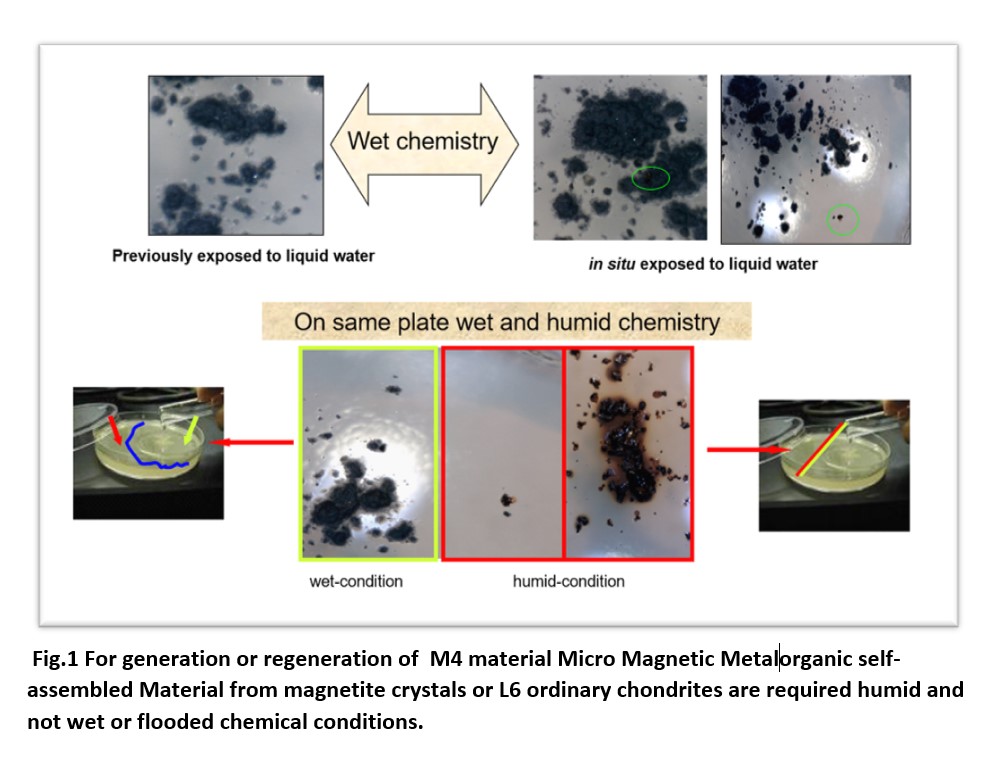
3. Summary and Conclusions
Searching for the very first instants of life on Earth, with several hypotheses in play [4], the challenge has been to replicate the conditions that could have allowed the emergence of early life to emerge. I developed a new approach to stimulate physicochemical processes that may have led to the emergence of the first life forms from inanimate matter on Earth or Earth-like planets via photo-metabolic pathways. My studies does not starts from ground zero, but provide evidence of non-enzymatic catalysis that modifies sugars, aminoacids, urea and other molecules produced in the prebiotic environments on the planets or satellites of our solar system by investigating the effect of physico-chemical stress on the formation of the metal-organic material M4 [3].
References
[1] del Gaudio, R.: Understanding the key requirement and the conditions that sparked life on Earth and beyond:clues and new knowledges supporting MuGeRo hypothesis., Europlanet Science Congress 2020, online, https://doi.org/10.5194/epsc2020-167, 2020.
[2] del Gaudio, R.: Transition from Non-living to living Matter: can integration of MuGeRo hypothesis and synthetic prebiotic biology laboratory approach shed light on the origin of Life? , Europlanet Science Congress 2021, online, 13–24 Sep 2021, EPSC2021-347, https://doi.org/10.5194/epsc2021-347, 2021.
[3] Geraci, G., D’Argenio, B., del Gaudio R. Patent US9328337 B2, granted, 2016.
[4] Bartlett, S. and Wong, L., Defining Lyfe in the Universe: From Three Privileged Functions to Four Pillars Life 2020, 10(4), 42; https://doi.org/10.3390/life10040042
How to cite: del Gaudio, R.: From molecular simplicity to the emergent complexity of earliest life: investigating key features and the role of physicochemical periodic stress on Earth and on Earth-like planets., Europlanet Science Congress 2022, Granada, Spain, 18–23 Sep 2022, EPSC2022-299, https://doi.org/10.5194/epsc2022-299, 2022.
Since the detection of the first exoplanet orbiting a star like the Sun, the University of Geneva has been at the forefront of exoplanet research. Starting from an extensive expertise in planet detection (with radial velocity), the observatory is also now an important actor in the atmosphere characterization of exoplanets (e.g. Ehrenreich et al. 2020). Today the focus is shifting towards the atmospheric characterization of small temperate planets, such as Proxima-b and the TRAPPIST-1 planets. The university is therefore actively participating to the instruments RISTRETTO@VLT and ANDES@E-ELT which aim at characterizing the atmosphere of Proxima-b (among other goals) using a technique based on high-contrast imaging and high-resolution spectroscopy. One of the objectives of these instruments is to detect biosignatures in the atmosphere of rocky temperate planets. However, to be able to correctly identify a biosignature, one needs to be able to identify false positives. So, one needs to know how the atmosphere interacts with planetary interior, with incoming stellar radiation, and with many different other processes. A multi-disciplinary approach is therefore necessary.
Recently, and following the 2019 Nobel prize in physics attributed to Michel Mayor and Didier Queloz for the discovery of 51 Peg b, the University of Geneva decided to create a faculty center: “Centre pour la Vie dans l’Univers” in French or “Center for Life in the Universe” (https://www.unige.ch/sciences/cvu/). The members of the center include experts in astrophysics, geophysics, environmental physics, chemistry, climatology and biology. The center aims at leading interdisciplinary projects on the origin of life on Earth and the search for life in our solar system and in exoplanetary systems to contribute to the world research on fundamental questions: How did life emerge and how did it diversify on Earth? Is the Universe full of life? What is the nature of life? How can we detect life elsewhere than on Earth?
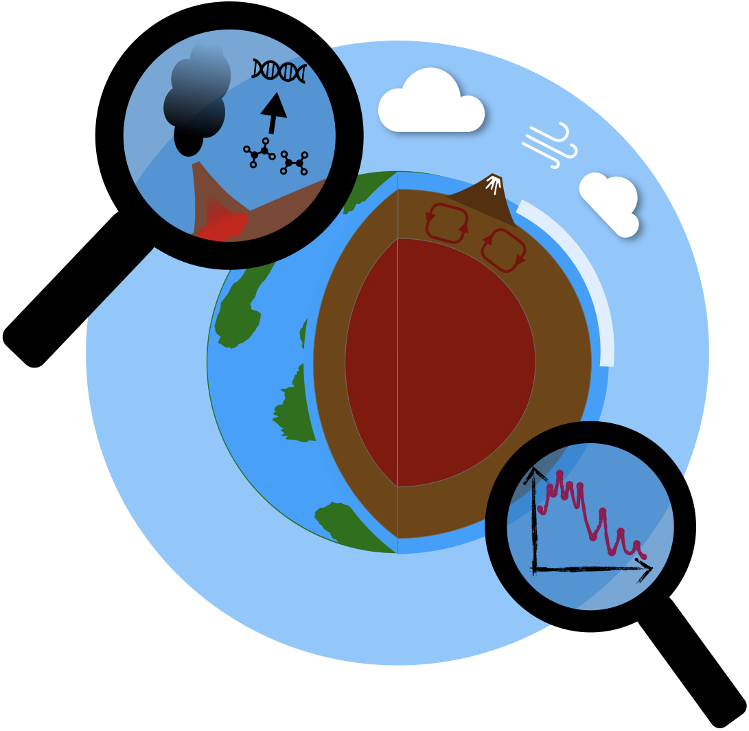
Several projects are starting and will start in the near future in the center on the following topics:
- The rise of molecular complexity on primitive Earth
- Multi-stability of climates and habitability
- Evolution under extraterrestrial conditions
- The atmosphere as a mirror for geological processes
I will present these new interdisciplinary scientific projects, with an increased focus on the second and third ones which are already underway.
How to cite: Bolmont, E., Ehrenreich, D., Kasparian, J., Ibelings, B., McGinnis, D., Winssinger, N., Caricchi, L., Castelltort, S., and Mueller, A.: From experimental evolution to climate simulations: the projects of the newly created Center for Life in Universe, Europlanet Science Congress 2022, Granada, Spain, 18–23 Sep 2022, EPSC2022-386, https://doi.org/10.5194/epsc2022-386, 2022.
We used the Planetary Spectrum Generator (PSG) [1] a radiative transfer suite, with the goal of simulating spectra from observations of Venus, Mars and Jupiter, searching for minor chemical species.
For Venus, sulphur dioxide (SO2) absorption lines were detected and its abundance constrained, by comparing simulations with observations by the Texas Echelon Cross Echelle Spectrograph (TEXES) spectrograph, around 7.4 μm [2]. The mean abundance of SO2 was constrained to 120 ppb, using the Optimal Estimation Method [3] and a line-depth ratio method [2] independently, in agreement with 50-175 ppb obtained by Encrenaz et al [2]. Phosphine (PH3) was not detected in the comparison between simulation and TEXES Infrared (IR) observations [4], around 10.5 μm, due to the presence of a strong telluric water band in the spectra.
For Mars, both a positive and a negative detection of methane were reanalyzed using PSG simulations with the goal of constraining the methane abundance. The related spectra observations in the IR, around 3.3 μm, report, respectively, to the Mars Express (MEx) [5] and ExoMars [6] space-probes.
For Jupiter, the detection of ammonia, phosphine, deuterated methane and methane was studied, by comparing simulations with IR observations by the Infrared Space Observatory (ISO), around 7-12 μm. [7]. The next step is focused in the determination of the abundances of the previous species. Independent simulations will be performed using PSG and the NEMESIS state-of-the-art radiative transfer suite [8]
Funding: This research was funded by the Portuguese Fundacao Para a Ciencia e Tecnologia under project P-TUGA Ref. PTDC/FIS-AST/29942/2017 through national funds and by FEDER through COMPETE 2020 (Ref. POCI-01-0145 FEDER-007672).
Aknowledgments: We credit Thérèse Encrenaz, from LESIA, Observatoire de Paris, for all the support and fruitful discussion; Geronimo Villanueva, from NASA-Goddard Space Flight Center, for discussing issues regarding PSG; Marco Giuranna, PI of the PFS instrument of Mars Express (ESA), Alejandro Cardesín, from ESAC-ESA, Ann Carine Vandaele, PI of the NOMAD instrument of ExoMars (ESA) and Séverine Robert, from the ExoMars team, for all the support regarding Mars dedicated research; Gabriella Gilli (IAA), for the collaboration regarding the LMD-VGCM model; Patrick Irwin, from the University of Oxford (UK), for the collaboration under the NEMESIS radiative transfer code; Asier Munguira, from the University of the Basque Country, for his availability to discuss atmospheric research methods in the context of the present work.
References
[1] Villanueva et al. 2018, Journal of Quantitative Spectroscopy and Radiative Transfer
[2] Encrenaz et al. 2012; Astronomy & Astrophysics
[3] C. D. Rodgers. Inverse methods for atmospheric sounding: theory and practice. World Scientific, 2008
[4] Encrenaz et al. 2020; Astronomy & Astrophysics.
[5] Giuranna et al. 2019; Nature
[6] Korablev et al. 2019.; Nature
[7] Encrenaz et al. 1999 ; Planetary and Space Science
[8] Irwin et al. 2008 ; Journal Of Quantitative Spectroscopy And Radiative Transfer
How to cite: Dias, J., Machado, P., Ribeiro, J., and Freire, C.: Atmospheric evolution and the search for species of astrobiological interest in the Solar System – Case Studies using the Planetary Spectrum Generator, Europlanet Science Congress 2022, Granada, Spain, 18–23 Sep 2022, EPSC2022-437, https://doi.org/10.5194/epsc2022-437, 2022.
Introduction
A planet that harbor water in a liquid state becomes as a study subject for its habitability evaluation. Water is the only known solvent in which the reactions for life as we know it take place, while is also a sink of molecules that include bio-essential elements such as carbon.
On Earth, oceans are reservoirs of CO2 and CH4 and, along with other molecules (H2S, N2, etc.) may be encapsulated in minerals of clathrate hydrates (thereafter clathrates) under high pressure and low temperature conditions [1]. Water molecules begin to arrange in space and join through hydrogen bonds, constructing a tridimensional crystal network that host gases inside by the van der Waals interaction forces [2]. This physical and chemical conditions required for clathrate deposits formation are found on Earth in continental margins and polar regions [3].
On Europa and Enceladus moons, clathrate deposits would not only be found in the seafloor, but also floating into oceans [4, 5, 6]. On Titan, as well as on Europa, they might form part of the composition of water-ice crust [7, 8], whereas on Ganymede and Pluto they may constitute some global layers of its internal structure [9, 10].
Clathrate formation and dissociation would play a role in geological processes and, above all, in (bio)-geochemical cycles of these planetary bodies. As clathrates are sinks of carbon and other chemical elements essential for life, the dissociation of these minerals by changes in physical chemical conditions would release gases into Europan and Enceladus´ oceans, enabling to promote favourable conditions for development of a hypothetical chemolithoautotrophic life [11]. However, gases could also be sequestrated again as carbonates or another salts due to reactions between them and rocky core in the water-rock interphase.
On Earth, encapsulated gases into clathrate structure may be metabolized by organotrophs [15] and/or by a consortium of methanotrophic archaea and sulfate-reducing bacteria after its dissociation [11, 16]. As a consequence carbonate precipitates, known as clathrite [17] because it records the past presence of these deposits. The aim of this study is to simulate the abiotic clathrite formation process under ocean-world-environmental-conditions when there are calcium saturation during clathrate formation and dissociation.
Methodology
For the experiments, we used a high-pressure simulation chamber made of stainless steel (volume capacity 67 ml) which is connected to a tank of CO2 (gas). It is coupled with a thermocouple and pressure sensor to monitor temperature and pressure parameters and with a Raman spectrometer to analyse phase changes. We filled the high-pressure cell with crushed ice made of 7.4 wt% Ca(OH)2 dissolution. The chamber was pressurized at 30 bar and then temperature was reduced down to 260 K. Once CO2 clathrates were formed, the chamber was heated slowly up to 284 K. We studied the synthesis process of clathrite, taking in situ Raman spectra with a 532 nm laser at every pressure and temperature change.
Results
Carbonate precipitation occurred since CO2 was injected to the chamber. The final product phase obtained was calcite. Nevertheless, during experiment of clathrate formation and dissociation, carbonate structure took diverse polymorphs of calcium carbonate different from pure calcite, aragonite and vaterite structures. This was evidenced by the spectral signature within the ranges of 1069.42-1087.75 cm-1 and 709.26-731.94 cm-1 for stretching and bending vibration of the CO32- ion respectively and 150.30-160.62 cm-1, 194.17-211.97 cm-1 and 280.03-289.94 cm-1 for lattice modes.
Acknowledgments
We thank project PID2019-107442RB-C32 funded by MINECO. Ana de Dios is supported by the AEI pre-doctoral contract under the project MDM-2017-0737-19-1.
References
[1] Rajput and Thakur (2016) in Geological Controls for Gas Hydrates and Unconventionals, Elsevier. [2] Sloan (1998) in Clathrate hydrates of natural gases, CRC Press. [3] Ruppel and Kessler (2017) Rev. Geophys., 55, 126-168. [4] Bouquet et al. (2015) Geophys. Res. Lett., 42, 1334-1339. [5] Prieto-Ballesteros et al. (2005) Icarus, 177, 491-505. [6] Boström et al. (2021) Astron. Astrophys. 650:A54. [7] Choukroun et al. (2010) Icarus, 205, 581-593. [8] Bouquet et al. (2019) ApJ, 855 (14). [9] Izquierdo-Ruiz et al. (2020) ACS Earth Space Chem., 4 (11), 2121-2128. [10] Kamata et al. (2019) Nat. Geosci., 12, 407-410. [11] Carrizo (2022) Astrobiology, 22 (5), DOI:10.1089/ast.2021.0036. [12] Choukroun et al. (2010) Icarus, 205, 581-593. [13] Fagents (2003) J. Geophys. Res., 108, 5139. [14] Bouquet et al. (2015) Geophys. Res. Lett., 42, 1334-1339. [15] Snyder et al. (2020) Sci. Rep., 10, 1876. [16] Bohrmann et al. (2002) Proc. Fourth Int. Conf. Gas Hydrates, Yokohama, Japan, 102-107. [17] Kennet and Fackler-Adams (2000) Geology, 28, 215-218. [18] Wehrmeister et al. (2007) J. Gemmol., 37(5/6), 269-276. [19] Eaton-Magaña et al. (2021) Minerals, 11, 177. [20] Chen et al. (2015) Chem. Eng. Sci., 138, 706-711.
How to cite: de Dios Cubillas, A., Muñoz Iglesias, V., and Prieto Ballesteros, O.: Abiotic clathrite synthesis from CO2-clathrate under ocean world conditions, Europlanet Science Congress 2022, Granada, Spain, 18–23 Sep 2022, EPSC2022-544, https://doi.org/10.5194/epsc2022-544, 2022.
Intro
Kerogen is insoluble, macromolecular organic matter in sedimentary rocks. Kerogen is highly abundant on Earth, making this subsurface carbon reservoir larger than any single surface carbon reservoir. Based on the origin of the organic matter, four types of kerogens are distinguished, with each their own chemical composition (Fig. 1). Type 1 is derived from fresh water algae, type 2 from marine algae, type 3 from terrestrial vascular plants, and type 4 is partially decomposed organic matter. Next to the abundance of kerogens on Earth, kerogens also comprise 70% of the organic material in carbonaceous chondrites (Sephton, 2002), and similar macromolecular organics have been discovered on the surface of Mars (Eigenbrode et al., 2018). As kerogens consist of large, insoluble, non-hydrolysable complexes (>1kDa), they are difficult for many microorganisms to access as an energy or carbon source (Vandenbroucke, 2003; Petsch et al., 2001). On the contrary, macromolecular organic material had been shown to be inhibitory to biofilms through occlusion of the biofilm surface (Freeman and Lock, 1992).
There is little understanding in the interaction of microorganisms with macromolecular, kerogenous material. This understanding is important as kerogenous material is a large carbon reservoir on Earth, and microbial degradation could impact the global carbon cycle with influences for climate change. Further, as kerogenous material is highly abundant in carbonaceous chondrites, and macromolecular material has been found on the surface of Mars, potential microbial usage of this material could have astrobiological implications. A proxy for extraterrestrial macromolecular, kerogenous material is kerogen embedded in rocks on Earth. In this research, we investigated the influence of each of the four kerogen types in rocks on the growth of an anaerobic microbial community.
Methods
An anaerobic microbial community capable of growth with a carbonaceous chondrite as the sole carbon and energy source as described in Waajen et al. (2022) was used. This community was grown for 11 days in microcosms containing liquid M9 medium with acetate and powdered rocks. Four types of rocks were tested, either shale or coal, with each rock sample containing one of the four kerogen types. At the end of the growth period, the community composition was determined by 16S amplicon sequencing. We also investigated the production of CO2, CH4 and H2 in the microcosms.
Results and discussion
Kerogen type 1 and 2 enhanced microbial growth to some extent. The microbial community composition did not change in the presence of kerogen type 1, but did change significantly during growth on kerogen type 2. This indicates that the growth of only a subset of the microbial community was enhanced by the presence of kerogen type 2, while another part of the community was not. We are currently investigating the metabolisms present in these environments, which could give an indication as to which compounds in these rocks will have influenced the growth of the community.
Kerogen type 3 did not enhance microbial growth, which could be explained by the abundancy of phenols in this type of kerogen. Phenols can be inhibiting in higher concentrations (Van Schie and Young, 1998).
Since this community has already been shown to grow on carbonaceous chondrite, growth enhancement on kerogen type 4 was to be expected, since this type is the closest analogue to macromolecular organics in meteorites (Matthewman et al., 2013). However, the community changed significantly during the growth in the presence of kerogen type 4, indicating that there are still significant differences between these environments. Further, kerogen type 4 is considered the most inert type of kerogen, containing mainly consisting polycyclic aromatic hydrocarbons (PAHs). Small PAHs can be degraded by microorganisms (Bamforth and Singleton, 2005), but it remains unknown whether the larger PAHs that are found in space can be used by microorganisms.
In addition to kerogens, shales and coal contain a small fraction of soluble organic material that could have been used by the microorganisms. Other compounds in shales and coals, such as metals, could also have influenced microbial growth. Further investigation in the type of material accessed by the microorganisms is needed to understand whether inert material from this type of kerogen can be microbially degraded.
No biological H2, CO2 or CH4 production was observed, which could be caused by the absence of certain metabolisms, or the direct consumption of these gases by other microorganisms. Alternatively, the low concentration of microorganisms in the microcosms could also have resulted in the lack of an observable production of these gases. We are currently analysing microbial community composition to indicate the presence of metabolisms which could produce these gases.
The potential of kerogenous material enhancing microbial growth has implications for the potential of life on Mars and in the presence of meteorites. The enhancement would indicate that the presence of macromolecular organic material in these environments would increase the habitability of these environments. Additionally, the potential degradation of kerogens has implications for carbon cycling on Earth, with the potential of the degradation of a large carbon reservoir. The entry of this stored carbon to the carbon cycle would have a large impact on climate change and should be further investigated.
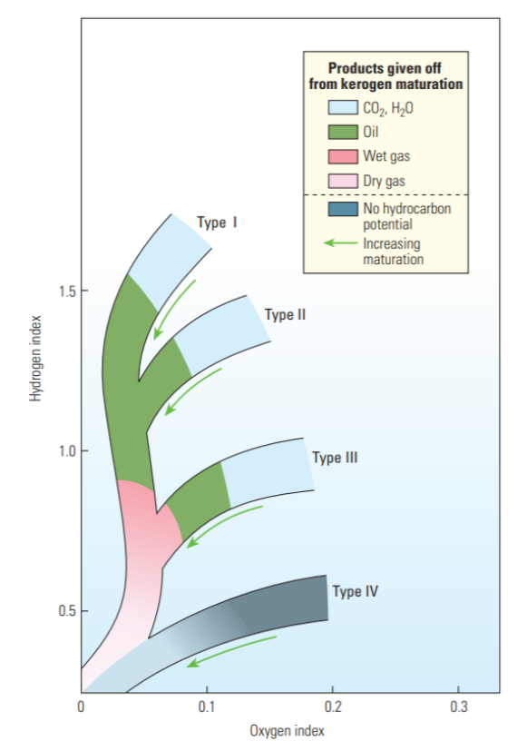
Figure 1: Chemical characteristics of the four kerogen types indicating the thermal maturation and products that can be given off for human oil and gas use. The hydrogen index is the H/C ratio, the oxygen index is the O/C ratio. Taken from McCarthy et al., 2011.
References
References
Bamforth et al., Journal of Chemical Technology & Biotechnology (2005).
Eigenbrode et al., Science (2018).
Freeman et al., Applied and Environmental Microbiology (1992).
Matthewman et al., Astrobiology (2013).
McCarthy et al., Oilfield Review (2011).
Petsch et al., Science (2001).
Sephton, Natural product reports (2002).
Vandenbroucke, Oil & gas science and technology (2003).
Van Schie et al., Applied and environmental microbiology (1998).
Waajen et al., Astrobiology (2022).
How to cite: Waajen, A. C., de Wit, W., Edgar, J. O., Telling, J., and Cockell, C. S.: Different forms of kerogenous carbon shape the growth and composition of anaerobic microbial communities, Europlanet Science Congress 2022, Granada, Spain, 18–23 Sep 2022, EPSC2022-1108, https://doi.org/10.5194/epsc2022-1108, 2022.
Introduction
In environments where it is difficult for life to function, microbial organisms tend to inhabit pockets of locally favorable climatic conditions. Micro-climates conducive to the persistence of life in an otherwise inhospitable environment – “refugia” – are spatially restricted and can be < centimeters in extent [1], [2]. Refugia may have been (and perhaps still are) perennially prevalent on Mars where conditions were likely never globally favorable to life for sustained periods of time [3]. The tendency for refugia to be small means that it may be difficult to locate features that could have served (or perhaps still do serve) as refugia for microorganisms on Mars. The spatial distribution of refugia in extreme environments across larger geographic extents is often non-random and may depend on many factors, biotic and abiotic [4]–[6]. Understanding patterns that refugia follow across larger geographic contexts as well as particular geologic phenomena (e.g., volcanic vents, dikes, stress fields) that are commonly associated with refugia may provide a way to infer regions of astrobiological interest, even if the specific, small, habitable patches (refugia) are below the resolving power of orbital instruments [6]. Here, we explore a case study of two terrestrial habitats in salt-encrusted paleo-lake basins (salars) in the Atacama and Altiplano of Chile to assess their characteristics and what factors are common between them. The Neogene salars of the Atacama and Altiplano are perhaps the best analogs on Earth for the Noachian/Hesperian salt-encrusted paleo-lakes of Mars [4], [7]–[12].
Evaporite habitats at Salar Grande and Salar de Pajonales
Salar Grande hosts decimeter scale nodules made of halite that serve as refugia for endolithic microbes [9]. [1] proposed a model to describe the evolution of nodules in halite-encrusted salars at the edges of polygonal features. To briefly summarize their model, halite nodules initiate at polygon edges in a salar with active ground water. Growth continues after ground water activity ceases as winds drive a moisture gradient, along which brines travel, toward the apex of the relatively higher relief nodules where more halite is deposited (Fig 1). The action of brines in halite nodules generates porosity at multiple spatial scales (nanometers to millimeters), contributing positively to their habitability [1].
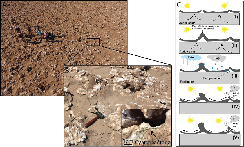
Fig. 1 Halite nodules at Salar Grande. A) Drone-view of nodules and nodule clusters. Humans for scale. B) Close up of halite nodule showing endolithic community. C) Halite nodule evolution from [1].
Like Salar Grande, Salar de Pajonales hosts endoliths in refugia habitats. In a gypsum-covered region of Salar de Pajonales, alabaster (a high-porosity polymorph of gypsum) is the most reliable indicator for the presence of life [4]. Alabaster refugia are most commonly found associated with decimeter- to meter-tall ridges and domes [6], [10]. The domes and ridges form via water-related processes: hydration/dehydration cycles, volume changes associated with mineral precipitation from brines, and/or efflorescence deliquescence [10]. The formation of alabaster is likely predicated on the action of the near-surface water that drives the formation of ridges and domes (Fig. 2), though microbial activity may play a role as well [4]. Therefore, at Salar de Pajonales water activity generates positive topographic salt constructs and physiochemical changes to gypsum (formation of high-porosity alabaster) that foster an environment favorable to life.
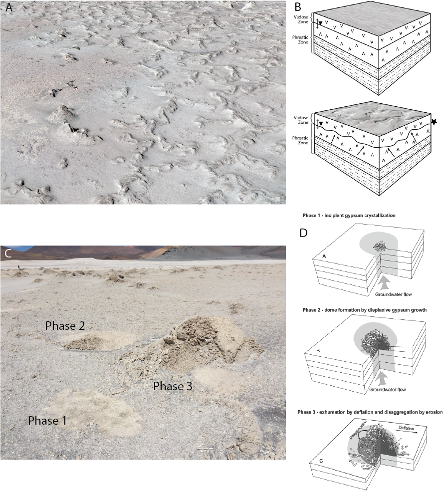
Fig. 2 Models of ridge and dome formation at SdP. A) Drone-perspective view of ridges at SdP. B) Model for ridge formation from [10] involving volume change at the phreatic-vadose zone interface. C) Image of domes at SdP in different stages of development. D) Possible model of gyspsum dome formation from [16].
Discussion
Across two salt-encrusted environments, one in the Atacama and the other in the Altiplano, with distinct evaporite mineralogy (halite versus gypsum), the activity of water resulted in decimeter- to meter-tall topographic constructs with nanometer- to millimeter-scale porosity conducive to the persistence of endoliths. We hypothesize that decimeter- to meter-tall topographic constructs (as opposed to erosional remnants or boulders) may be general indicators for relatively enhanced habitability in salt-encrusted paleo-lake basins because they require water to form. Although refugia – such as the precise location of endoliths in halite nodules or alabaster in gypsum domes and ridges – may not be observable from orbit, decimeter- to meter-scale salt constructs may be possible to identify with HiRISE or future orbital imagers with higher resolving power [6]. Chloride basins should be the targets of high-resolution imaging campaigns and efforts should be made to distinguish salt constructs from erosional remnants, boulders, and other relative topographic highs with which they could be confused. Salt constructs may be one of the few features, other than (fossil) hydrothermal vents, that have a high potential to both host and preserve microbial organisms, and that are specific targets, possibly identifiable from orbit, to which a rover could be driven. These characteristics make them attractive targets for future missions to Mars.
Reference:
[1] O. Artieda et al., 2015, doi: 10.1002/esp.3771.
[2] L. Hays, “NASA Astrobiology Strategy.” 2015.
[3] R. Wordsworth et al., 2021, doi: 10.1038/s41561-021-00701-8.
[4] K. Warren-Rhodes et al., Nature Astronomy. in review.
[5] M. S. Phillips et al., Astrobiology, in review.
[6] K. A. Warren-Rhodes et al., 2019. doi: 10.3389/fmicb.2019.00069.
[7] M. M. Osterloo, et al., 2010, doi: 10.1029/2010JE003613.
[8] T. D. Glotch, et al., 2016, doi: 10.1002/2015JE004921.
[9] A. F. Davila et al., 2008, doi: 10.1029/2007JG000561.
[10] N. W. Hinman et al., 2022, https://www.frontiersin.org/article/10.3389/fspas.2021.797591
[11] N. A. Cabrol et al., 2007, doi: 10.1029/2006JG000298.
[12] E. K. Leask and B. L. Ehlmann, 2022, doi: 10.1029/2021AV000534.
[13] A. Szynkiewicz, et al., JGR, vol. 115, 2010.
How to cite: Phillips, M., Warren-Rhodes, K., Hinman, N., Moersch, J., Hofmann, M., McInenly, M., Davila, A., and Cabrol, N.: Salt constructs in paleo-lake basins as high-priority astrobiology targets., Europlanet Science Congress 2022, Granada, Spain, 18–23 Sep 2022, EPSC2022-1188, https://doi.org/10.5194/epsc2022-1188, 2022.
Molecular oxygen (O2) paired with a reducing gas is regarded as a promising biosignature pair for atmospheric characterization of terrestrial exoplanets. In circumstances when O2 may not be detectable in a planetary atmosphere (for instance, at mid-IR wavelengths) it has been suggested that O3, the photochemical product of O2, could be used as a proxy to infer the presence of O2. While O3 is not directly produced by life, it plays an important role in habitability as the ozone layer is the primary source of UV shielding for surface life on modern Earth. However, O3 production is known to have a nonlinear dependence on O2, as well as being strongly influenced by the UV spectrum of the host star. To evaluate the reliability of O3 as a proxy for O2 we used Atmos, a 1D coupled climate/photochemistry code, to study the O2-O3 relationship for "Earth-like'' habitable zone planets around a variety of stellar hosts (G0V-M5V) for O2 abundances from 0.01%-150% of the Present Atmospheric Level (PAL) on modern Earth. We studied how O3 emission features for these planetary atmospheres varied for different O2 and O3 abundances using the radiative transfer code PICASO. Overall we found that the O2-O3 relationship differed significantly around different stellar hosts, with different trends for hotter stars (G0V-K2V) than cooler stars (K5V-M5V). Planets orbiting hotter host stars experience an increase in O3 when O2 levels are initially decreased from the present atmospheric level, with maximum O3 abundance occurring at 25-55% PAL O2. Although this effect may seem counterintuitive, it is due to the pressure dependency on O3 production, as with less atmospheric O2 incoming UV photons capable of O2 photolysis are able to reach lower (denser) regions of the atmosphere to spark O3 formation. This effect is not present for planets orbiting our cooler host stars (K5V-M5V), as the weaker incident UV flux (especially FUV flux) does not allow O3 formation to occur at dense enough regions of the atmosphere such that the faster O3 production outweighs a smaller source of O2 from which to create O3. As a result, for cooler host stars the O3 abundance decreases as O2 decreases, albeit nonlinearly. Interpretation of O3 emission spectral features was found to require knowledge of the atmosphere’s temperature profiles -particularly the temperature differences between the planetary surface and stratospheric temperature- which are highly influenced by the amount of stratospheric O3. Planets experiencing higher amounts of incident UV have more efficient O3 production and UV absorption leading to larger stratospheric temperature inversions, and therefore shallower emission features. Overall it will be extremely difficult (or impossible) to infer precise O2 levels from an O3 measurement, however, with information about the UV spectrum of the host star and context clues, O3 will provide valuable information about potential surface habitability of an exoplanet.
How to cite: Kozakis, T., Mendonça, J. M., and Buchhave, L. A.: Is ozone a reliable proxy for molecular oxygen?, Europlanet Science Congress 2022, Granada, Spain, 18–23 Sep 2022, EPSC2022-1267, https://doi.org/10.5194/epsc2022-1267, 2022.
TP17 | Planetary field analogues for Space Research
1 Introduction
The Finnish Meteorological Institute (FMI) has developed relative humidity instruments for several Mars lander missions. Calibration of these instruments can be challenging due to the required temperature, pressure and humidity conditions that can be reliably simulated by only a few laboratories. Humidity measurements in Martian conditions have been previously performed for these instruments in the FMI’s laboratory and the Michigan Mars Environmental Chamber (MMEC) at the University of Michigan. A new measurement campaign was performed at the Planetary Analog Simulation Laboratory (PASLAB) of the German Aerospace Center (DLR) during autumn 2020 and spring 2021. The campaign included three ground reference models (REF) of FMI’s relative humidity instruments: REMS-H of the MSL Curiosity rover [1], MEDA HS of the Mars 2020 Perseverance rover [2] and METEO-H developed for the ExoMars 2022 surface platform [3]. All three instruments are based on HUMICAP® capacitive thin-film polymer sensors by Vaisala as well as Vaisala’s ASIC technology. REMS-H has three HUMICAP sensor heads, while MEDA HS and METEO-H both contain two newer types of HUMICAP sensors which provide a larger dynamic capacitance range and include integrated resistive PT1000 sensors for measuring the temperature of the sensor head. The REF models of each instrument are identical to the flight models and have gone through testing and calibration campaigns at FMI together with the flight models.
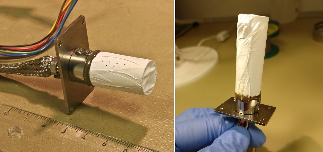
Figure 1: REMS-H (left) of the MSL Curiosity rover and MEDA HS (right) of the M2020 Perseverance rover. METEO-H for ExoMars 2022 is identical to MEDA HS. The electronics and sensor heads are located on a PCB inside a cylindrical Faraday shield. The Faraday shield is covered with PTFE membrane filter to protect the sensor from dust.
The main purpose of the measurement campaign at the DLR was to obtain calibration data in multiple humidity points in CO2 within the instruments’ operational temperature and pressure ranges. The instruments have been calibrated at the FMI using two humidity points in CO2, resulting in satisfactory quality but a notable calibration uncertainty. The new multi-point data are used for complementing the calibration of MEDA HS and METEO-H flight models, as well as to check REMS-H calibration.
2 Test setup
The DLR PASLAB facility, designed to simulate Martian near-surface atmospheric conditions, is used for habitability-related investigations and sensor studies [4][5]. In this measurement campaign the environmental conditions were controlled in terms of gas type, pressure, temperature and relative humidity. The setup is described in Figure 2. The instruments were enclosed in the same measurement chamber as has been used in the FMI’s laboratory (see Figure 3), and the chamber was connected to the environmental control system. As part of the DLR’s own experiment, another chamber with humidity sensors was connected to the system for simultaneous measurements, with one sensor also placed inside the FMI’s chamber for comparison.
The measurements were performed at stable temperature points between -70 °C and -30 °C and pressure points ranging from 5.7 hPa to 9.8 hPa in CO2 gas. At each temperature and pressure combination, a sequence of stable humidity points was run by an automatic program, increasing the humidity in steps from the driest point to the highest humidity and back. Some continuous measurements were also performed in changing humidity. At the end of the campaign, a different gas mixture imitating the true Martian atmospheric composition was tested to investigate possible effects on the sensor behavior.
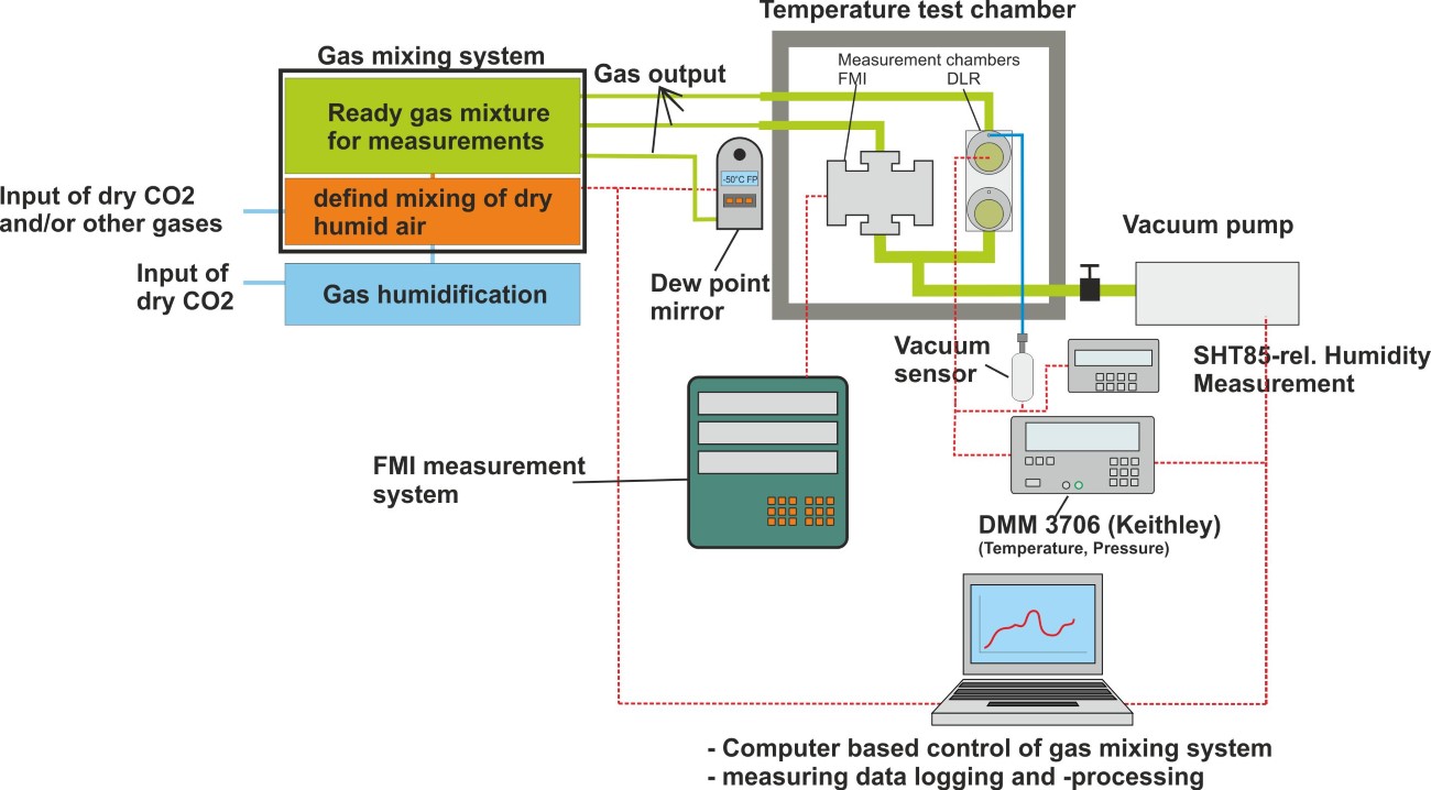
Figure 2: Setup of the environmental control and measurement system at the DLR PASLAB. Credit: DLR.
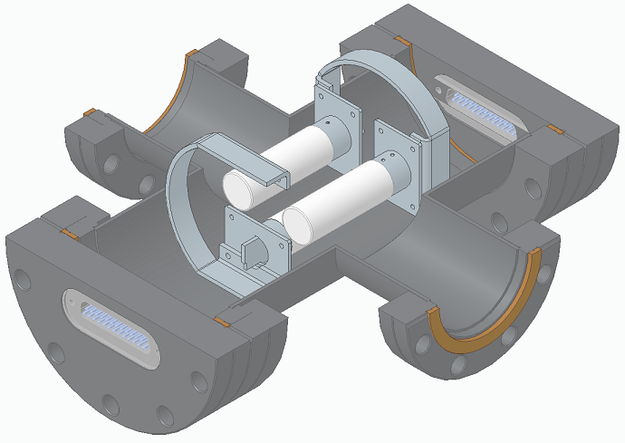
Figure 3: Cutaway illustration of the measurement chamber with the three FMI's ground reference models inside.
3 Campaign outcome
The measurement campaign was completed in May 2021 with successful outcomes. All planned temperature and pressure combinations were performed once or twice with a sufficient range of humidity points. However, at -30 °C temperature only points up to about 30 %rh could be achieved due to system limitations. We obtained a comprehensive set of stable humidity point data for each of the humidity sensors, as well as some data in changing humidity. Figure 4 shows the stable humidity points measured by one HUMICAP sensor from each instrument. The results are as expected: the temperature dependence is observed as a clear spread of capacitance readings and the pressure effect as a slight dispersion. Using the Martian-like gas composition did not seem to affect the sensor behavior compared to pure CO2.
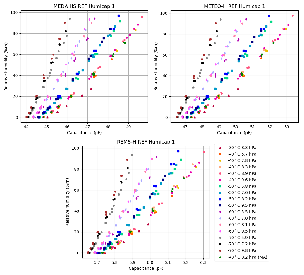
Figure 4: Selected measurement points in different temperature and pressure combinations shown for one HUMICAP sensor of each REF model: MEDA HS (upper left), METEO-H (upper right) and REMS-H (lower center). The y-axis represents the reference relative humidity in the measurement chamber and the x-axis the sensor output capacitance. Measurements in the Martian atmospheric gas composition are marked with green stars.
4 Conclusions
The humidity measurement campaign at the DLR PASLAB was performed between September 2020 and May 2021. As an outcome we obtained valuable datasets for MEDA HS, METEO-H and REMS-H ground reference models consisting of multiple relative humidity points over the sensors’ range from 0 %rh to 100 %rh in low pressure CO2. The results were in line with previous laboratory measurements of these instruments.
References
[1] Harri, A.-M. et al.: Mars Science Laboratory relative humidity observations: Initial results. J Geophys Res Planets 119, 2132–2147 (2014).
[2] Rodriguez-Manfredi, J.A. et al.: The Mars Environmental Dynamics Analyzer, MEDA. A suite of environmental sensors for the Mars 2020 mission. Space Sci Rev 217:3, 48 (2021).
[3] Vago, J. et al.: ESA ExoMars program: The next step in exploring Mars. Sol Syst Res 49, 518-528 (2015).
[4] Lorek A. and Koncz A.: Simulation and measurement of extraterrestrial conditions for experiments on habitability with respect to Mars. In Habitability of Other Planets and Satellites, vol. 28, 145–162 (2013).
[5] Lorek A. and Majewski J.: Humidity measurement in carbon dioxide with capacitive humidity sensors at low temperature and pressure. Sensors 18. (2018).
How to cite: Jaakonaho, I., Hieta, M., Genzer, M., Polkko, J., Lorek, A., Garland, S., de Vera, J.-P., and Harri, A.-M.: Relative humidity laboratory measurements in Martian atmospheric conditions, Europlanet Science Congress 2022, Granada, Spain, 18–23 Sep 2022, EPSC2022-819, https://doi.org/10.5194/epsc2022-819, 2022.
Introduction
Sedimentary deposits developed in High-Altitude Andean Lakes (HAAL) share some extreme and environmental characteristics that made them excellent analogues for planetary geology and astrobiology research. These conditions favor the development of a diverse and abundant microbial biota that influence mineral precipitation (e.g. carbonates) and the develpoment of microbially influenced sedimentary deposits typically know as stromatolites. To recognize and differentiate stromatolites from similar laminated deposits purelly formed by chemical processes is not straightforward, and Archean stromatolites are a good example. This makes HAAL good environmental analogues to study microbe-mineral proceeses, and the associated biosignatures. The recent findings of putative marginal lacustrine and delta deposits in the Jezero crater on Mars surface highlight the potential of these systems from and astrobiology perspective. The origin and characteristics of these martian carbonates is still unknown so the evaluation potential scenarios in comparable environmental conditions may shed some light into this uncertainties.
The Laguna Negra (a high altitude lake in Catamarca Province, Argentina) is an outstaning example of HAAL where an active microbial mat system and associated carbonate deposits is well developed. These are located in the mixing zone between groundwater spring-fed pools and the main lacustrine system. The Laguna Negra is a unique natural laboratory that fulfills the environmental criteria suggested for early Earth (Archean) and Mars (Noachian) where spectrum of biotic and abiotic process can be studied improving our ability to interpret the sedimentary record on our planet and beyond.
Geological setting
The Laguna Negra is a shallow hypersaline lake where the pH of the main lake and the groundwater springs feeding the lake fluctuates between ~6 and ~8 and salinity between ~320 and ~9 ppt respectively. The mixing zone between the main lake and groundwater is oversaturated with respect to calcite and aragonite. The carbonate belt consists of oncoids, stromatolites, and laminar crusts that are spatially localized in different zones and associated to different microbial mats systems and chemical conditions. Particularly interesting are the laminar crusts, developed in a zone where no significant microbial mats has been observed, but where a diversity of morphologies and microtextures has been recorded. Although interpreted as purelly chemically precipitated, unravelling the different processes that controls this morphological varibality is still challenging.
Oncoids, Stromatolites and Laminar crusts
Oncoids represented by concentrically laminated discs, spheres, and flattened domes (cm to dm in diameter) that can coalesce to form more complex structures and are typically associated with well-stratified diatom-rich microbial mats. The external surface surface can be smooth or can show pillar-like to shrub-shaped millimeter scale protrusions and ornamentations, particularly on the side affected by wind and currents. Oncoids are partially buried and can show lateral protrusions at the sediment–water and the air–water interface. Although oncoids are sub-spherical in shape, they can show asymmetric growth (bigger below the sediment–water interface). Complex lamination is also a result of oncoid rotation, particularly by cryoturbation and bioturbation.
Although water mixing, CO2 degassing, and evaporation are particularly important to trigger carbonate precipitation the influence of microbial mats is visible in the macromorphologies (differential growth within the anoxic zone related to metabolisms that increase alkalinity) and a diverse set of microtextures some of which are interpreted as microbially influenced.
Stromatolites more localized and represented by centimeter to decimeter-scale laminated structures (up to 25 cm) that typically have a planar or laminar to columnar shape. They are observed associated with dark colored microbial mats and usually are encrusting the upper surface of oncoids. The columnar structures are usually centimeter-sized. Internal lamination is irregular, overlapping, crenulated-micritic to micro-peloidal laminae that preserve abundant organic remains. These features are suggestive of microbially influenced texture.
Laminar crusts show a patchy distribution and represented by millimeter to decimeter carbonate crusts encrusting volcanic rocks, peloidal sediments as well as organic remains. Can also develop dome-shaped morphologies showing concentric growth patterns. These concentric structures can be slightly assymetrical, showing preferential growth towards the upper half (as opposed to oncoids). Oriented and elongated structures are common (by wind-driven currents in the lake). Plates and domes can be rotated and/or coalesce to form more complex structures or more extensive platforms along the lakeshore. The surface can be smooth or show dendritic to pustular patterns or protusions as well as travertine-like microterracetes.
Isopachous regular laminane is the most common building block, as stated showing a concentric pattern but it is worth mentioning that the wind-oriented structures, in cross-section, develop more complex micro-textures (shrub-like to dendritic/micro-stromatolite microfabrics) that resemble microbially influenced structures.
Given the absence of microbial mats, and the macro-morphologies and micro-textures described (e.g., lamina regularity and degree of inheritance, lack of organic remains within the lamina), these structures have been interpreted as predominantly chemically precipitated carbonates, triggered by oversaturation related to water mixing, strong CO2 degassing, and evaporation.
Final considerations
Both, physocochemical and microbial processes can contribute to a diverse range of morphologies and carbonate microtextures and it is not easy to urvanel their relative contributions. Oncoids, stromatolites and laminar crusts show some distinctive features that suggest some of the driving controls, but also some overlapping characteristics that may be difficult to discriminate. As an example, although laminar crusts generally show (in cross section) a strong lamina regularity, a more diverse set of microtextures can be produced by the influence of advective-diffusive processes, localized scarbonate precipitation, rotation due waves, and cryo-bioturbation, thus increasing lamina complexity that can be confused with microbially influenced textures. Possible origins of the carbonates recorded at Jezero crater, for example including carbonate crusts developed over the basaltic substrate, pore-vein-filling carbonate cements, reworked carbonate material, or even stromatolite-like structures. Although chemical biosignatures (trace element distribution and isotope fractionation) are central in the tool box of astrobiologists, to recognize the putative biogenicity of these carbonates it is necessary to combine chemical analysis with the information provided by the external macro-micro morphology and the internal macro and micro microfabric, something that may not be possible when dealing with rover or image based analysis on outcrops or with sample returned to Earth, where part of the context may be lost.
How to cite: Gomez, F., Matic, M., Perez Valdenegro, P., Boidi, F., and Mlewski, C.: High-Altitude Andean Lakes as Natural Laboratories for Planetary Geology and Astrobiology Research: The Laguna Negra case (Argentina), Europlanet Science Congress 2022, Granada, Spain, 18–23 Sep 2022, EPSC2022-822, https://doi.org/10.5194/epsc2022-822, 2022.
The icy satellites of the Solar System, such as Europa, Ganymede and Enceladus, show widespread evidence for brittle morphotectonic structures (fractures/faults) that provide insights to infer the kinematics and the mechanical properties of their crusts. Their investigation is pivotal for the understanding of the tectonic regimes responsible for their formation. In addition, stress-related structures represent potential conduits or enhanced pathways for fluid migration thus connecting the surface and the sub-crustal layers. Such processes are significant to understand internal processes of icy bodies. Their investigation is constrained at regional-scale coverage of the remote sensing imagery.
Glaciers and ice sheets represent optimal terrestrial analogues, showing deformation styles similar to those in the icy satellites, and being the excellent sites to further explore, verify and confirm what observed through remote sensing on the geology of icy satellites. Although the formation processes differ, the similarity of their structures at surface allows quantifying and predicting the state of deformation in the icy satellites at different scales of investigation.
The UPSIDES project aims to investigate and compare the tectonic structures of the glaciers with those on the icy satellites, by means of multi-scale approach of both remote-sensing and field survey.
We propose a structural investigation in the Russell and Isunguata Sermia glaciers, located at the western margin of the Greenland Ice Sheet. Their investigation attempts: i) to identify scaling laws between the tectonic structures measured in the glacier outcrops and their equivalent mapped on satellite images; ii) to relate and compare such scaling laws with structures mapped on deformed areas of the icy satellites; and iii) to infer the tectonic styles at local-scale on the icy satellites. The knowledge of the tectonic setting at local-scale and its comparison with that at regional-scale, allow us to better understand the tectonic process and to characterize structures that are exclusively identified at regional-scale (such as in the icy satellites).
In this contribution we present the preliminary results of the analyses of data collected during the field campaign conducted on July 2021 in Greenland, at the Russell and Isunguata Sermia Gl., in the Europlanet 2024 RI's Transnational Access field analogue in Kangerlussuaq.
Field measurements include the characterization of the ice brittle deformation (e.g., fractures and fault) by the quantification of their azimuth, dip, length, width, throw and spacing. This allow us to recognize the tectonic settings and regimes responsible for their formation. In parallel, we performed a structural mapping on satellite images, which cover the locations where the investigated outcrop occur, and we derived the attributes of the mapped structures. We performed then paleo-stress analyses of the data from both local- and regional-scale, which in turn have been related. The obtained results are consistent and suggest strike-slip kinematics. Such results are compared with areas that show similar tectonic setting on Ganymede and Europa and support the understanding of the possible local-scale setting at surface. In addition, the field data allow us to identify the structures that ease the fluid migration.
The obtained results from this project aim to contribute to advance the study of icy surface tectonics and will support the preparation of planetary programs, such as JUICE mission, for dedicated observations and target areas.
Acknowledgments: This project has received funding from the European Union's Horizon 2020 research and innovation programme under grant agreement No 871149. The activity has been realized under the ASI-INAF contract 2018-25-HH.0.
How to cite: Rossi, C., Cianfarra, P., Lucchetti, A., Pozzobon, R., Penasa, L., Munaretto, G., and Pajola, M.: Unravelling icy Planetary Surfaces: Insights on their tectonic DEformation from field Survey - UPSIDES, Europlanet Science Congress 2022, Granada, Spain, 18–23 Sep 2022, EPSC2022-874, https://doi.org/10.5194/epsc2022-874, 2022.
Introduction
Studying planetary field analog environments is a key point in order to define the physical and chemical parameters that favor life on Earth and other planets. Terrestrial hydrothermal springs have long been considered among the most significant planetary analogs searching for traces of life on Mars [1].
Hyperspectral data have been recognised to be more suitable for the detailed mapping and identification of rocks and minerals identification of land surface, especially for minerals [2].
Notwithstanding the technological advances, hyperspectral satellites are still poorly represented in spaceborne missions for Earth Exploration compared to multispectral ones. In this context, the Italian Space Agency (ASI) EO mission named PRISMA (PRecursore IperSpettrale della Missione Applicativa, [3]) offers a great opportunity to improve the knowledge about the scientific applications of spaceborne hyperspectral data.
PRISMA, launched in March 2019, includes a panchromatic and a hyperspectral camera with 239 spectral bands. Specifically, the PRISMA satellite comprises a high-spectral resolution Visible Near InfraRed (VNIR) and Short-Wave InfraRed (SWIR) imaging spectrometer, ranging 400-2500 nm, with 30 m ground sampling distance (GSD) and 5 m GSD for the panchromatic camera [4].
Our analysis with PRISMA images was mainly performed on an arid environment in a remote region of NE Ethiopia (Dallol; Long: 40.299351, Lat: 14.244367), representing an exceptional Mars analog due to diffuse hydrothermal alteration and the sulfate deposits evocative of past hydrothermal activity on Mars. This work aimed to obtain an identification map of minerals and their relative abundance using hyperspectral imaging to understand the potential of PRISMA as analog probe of Mars orbital instruments to detect and study possible analogs on Earth.
Study Area
Dallol is situated in the Danakil Depression, which is part of the East African Rift System. Principal geothermal features of the central crater area of Dallol are salt pillars, circular manifestations and acidic ponds. The northern and southern part is dominated by a salt dome structure and Salt pinnacles in the SW salt canyon area. The Black Mountain and the super-saline Black Lagoon, just south-southwest of Dallol, is an area of salt extrusions, geothermal manifestations and brine upflows.
One advantage of this area is that the nebulosity is generally low, in fact the image selected during the dry season has a cloud coverage percentage of less than 1%. A salt suite was deposited and re-worked by hydrothermalism in the selected site. The characteristic minerals of the area are: carbonate, halite, carnallite and bischofite, anhydrite, gypsum, native sulfur of hydrothermal origin [5; 6].
Flooding episodes from the Lake Assale to the north due to intense winds acting over the flat topography of the depression. The PRISMA SWIR Land/Water band combinations on the image selected, helped us to choose the region of interest around the Dallol area.
Operational Hyperspectral Processing
PRISMA images have three different levels of processing. Level 2C and 2D geolocated and atmospherically corrected images were used in this work and dated 21 August 2021. it is worth noticing that the images acquired on Dallol prior to the image selected for analysis had several preprocessing problems, particularly for stripe removal.
The operational hyperspectral processing is composed of three main processing steps: (1) dimensionality reduction; (2) endmember identification and (3) mineral map distribution and abundance estimation.
An unexpected result was obtained by applying an additional atmospheric correction, the Internal Average Relative Reflectance with Dark Subtraction, on the L2C image already corrected during the principal component analysis (PCA). The corrected atmospheric PCA allows better highlighting of geomorphological features.
As for step (1), since hyperspectral images are composed of hundreds of extremely correlated bands, it is possible, and indeed beneficial, to reduce the effective dimension of the input data by removing bad bands.
Step (2) was performed using the THOR Hyperspectral Material Identification (in ENVI 5.6) to identify unknown spectral signatures by comparing them with spectral libraries. This tool considers background statistics and image endmembers and can therefore provide accurate responses and spectra plots for rare or sub-pixel targets.
Finally, the Spectral Angle Mapper (SAM) and the Linear Spectral Unmixing (LSU) tools were adopted for step (3). SAM determines the spectral similarity between two spectra by calculating the angle between the spectra and treating them as vectors in a space with dimensionality equal to the number of bands. LSU is a standard technique for spectral mixture analysis that infers a set of endmembers and fractions of these, called abundances. The mineral distribution and the abundance maps are shown respectively in Fig.1 and Fig.2.
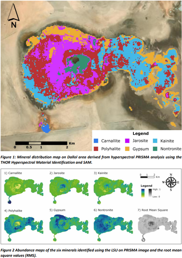
Conclusion
Six minerals have been recognised with the SAM classification from ENVI spectral library, in excellent agreement with the previous studies: carnallite, jarosite, kainite, polyhalite, gypsum and nontronite. The results confirm the mineralogical variability typical of the Dallol; in Fig.2, high mineral abundance values are shown in blue. The error calculated with the RMS is very low over the entire area of interest, except for the central zone where there are sulphur pools and therefore the presence of water does not favour this type of analysis.
To better constrain the mineralogical mapping, future work will be conducted by a field exploration campaign to collect spectral signatures to be added to the ENVI library used, which so far could not be organised due to the ongoing civil war in Dankalia.
To sum up, the study of terrestrial analogs can provide insights into the probable presence and nature of spring deposits on Mars, as well as help develop methods for classifying them from remote sensing data. PRISMA represents a valuable satellite for distinguishing not only the geometric characteristics of observed objects, but also the chemical-physical composition of the surface of the Earth.
References: [1] Walter, M.R. and Des Marais, D.J., 1993. Icarus 101:129–143 [2] Chang, C.I., 2007. John Wiley & Sons. 10.1002/0470124628 [3] Candela, L., et al. 2016. IEEE international geoscience and remote sensing symposium (IGARSS), 253-256. 10.1109/IGARSS.2016.7729057 [4] Loizzo, R., et al. 2019. IEEE (IGARSS), 4503-4506. 10.1109/IGARSS.2019.8899272 [5] Cavalazzi, B., et al. 2019. Astrobiology, 19(4), 553-578. 10.1089/AST.2018.1926 [6] López-García, J.M., et al. 2020. Frontiers in Earth Science, 7, 351. 10.3389/FEART.2019.00351
How to cite: Mancini, F., Tullo, A., Allemand, P., and Ori, G. G.: Mineral Identification and Abundance Mapping through the hyperspectral PRISMA images on the Dallol Planetary Analog, Europlanet Science Congress 2022, Granada, Spain, 18–23 Sep 2022, EPSC2022-983, https://doi.org/10.5194/epsc2022-983, 2022.
The identification of novel terrestrial sites that are analogous for other planetary bodies is an active area of research within astrobiology, because of the logistical and financial difficulties in obtaining extraterrestrial samples for analysis. Characterisation of potential analogue sites is undertaken to assess how accurately they represent a specific extraterrestrial environment. Analysing their physicochemical conditions and microbial communities are key components of these studies to understand what metabolisms would be viable in such environments.
One such novel analogue environment is the salt plains of Western Sahara. Western Sahara is one of the driest regions on Earth. It is located on the northwest coast of West Africa and is characterised by high UV exposure, low annual precipitation and water activity, subsurface water and high annual temperatures. These features make Western Sahara a potential analogue site for Mars during the Noachian-Hesperian transition period (3.5 – 3.8 Ga), when the atmosphere began to thin and surface water started evaporating (Warner et al., 2010), similar to other terrestrial deserts, such as the Atacama Desert and the McMurdo Dry Valleys.
The hypersalinity, aridity and high UV radiation levels of the Western Sahara salt plains would also be appropriate to study whether dissimilatory sulfur metabolisms would be viable in a Noachian-Hesperian Mars analogue environment. Dissimilatory sulfur cycling refers to the use of inorganic sulfur compounds for energy conservation and it has been recognised as a metabolic strategy of interest for putative martian life (Macey et al., 2020). On Earth, evidence from stable sulfur isotope fractionation has suggested this metabolism emerged early in the history of life (~3.5 Ga). During this period, the conditions on Mars were predicted as being more habitable than present-day, with an active magnetic field, thicker atmosphere and liquid water on the surface.
In this study, molecular and geochemical techniques were used to give first insights into the potential of the Western Sahara salt plains to serve as an analogue of Mars during the Noachian-Hesperian transition period. The microbiology was investigated through cultivation-independent and culture-dependent analyses of salt crystals, sediment and water samples obtained at three sites near Llaayoune (Fig. 1). The chemical nature of the samples was analysed through ion chromatography (IC) and inductively coupled plasma - optical emission spectrometry (ICP-OES).
The geochemical characterisation confirmed the high salinity of the samples and identified that sodium, potassium, magnesium and sulfur were the most enriched elements within all samples. Cultivation-dependent work resulted in the enrichment of a wide range of metabolic strategies from the samples including aerobic heterotrophs, phototrophs and sulfate-reducers. The enrichments from the salt were dominated by strains of Bacillus, whereas sulfate-reducing strains of Clostridium were isolated from the sediment samples. Microscope analysis of phototroph-selective media also indicated that algae and Cyanobacteria were successfully enriched from the samples. 16S rRNA amplicon sequencing results will also be presented to gain further in-depth understanding of the microbial community composition. Additionally, results from quantitative polymerase chain reaction (qPCR) experiment targeting sox and dsr genes will be presented to identify the abundance of genes specific for dissimilatory sulfur metabolisms within the samples.
Preliminary data shows that sulfur cycling is occurring in Western Sahara salt plains. Future characterisation of this environment will involve metagenomic analysis of the samples and genome sequencing of the isolates to identify the key metabolisms underpinning the survival and viability of the microbial community. Comparative studies with other Mars analogue environments will then be undertaken to identify metabolisms that may have been thermodynamically viable in ancient martian aqueous environments.
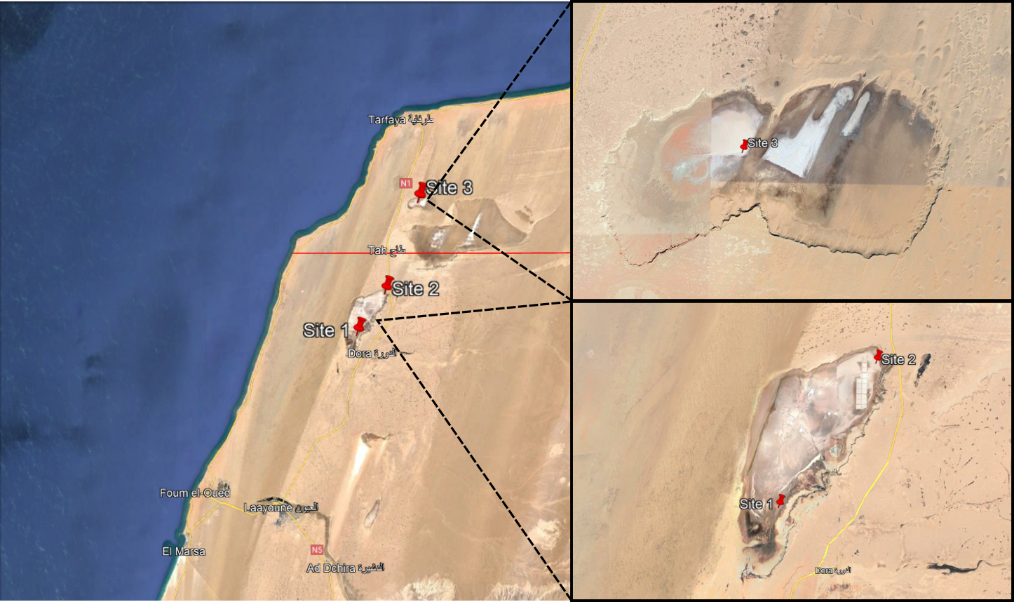
Figure 1. Location of the sample collection sites. Images were generated with Google Earth Pro.
References
Macey, M. C., Fox-Powell, M., Ramkissoon, N. K., Stephens, B. P., Barton, T., Schwenzer, S. P., . . . Olsson-Francis, K. (2020). The identification of sulfide oxidation as a potential metabolism driving primary production on late Noachian Mars. Scientific Reports, 10(1), 10941. https://doi.org/10.1038/s41598-020-67815-8
Warner, N., Gupta, S., Lin, S.-Y., Kim, J.-R., Muller, J.-P., & Morley, J. (2010). Late Noachian to Hesperian climate change on Mars: Evidence of episodic warming from transient crater lakes near Ares Vallis [https://doi.org/10.1029/2009JE003522]. Journal of Geophysical Research: Planets, 115(E6). https://doi.org/https://doi.org/10.1029/2009JE003522
How to cite: Ilieva, V., Stephens, B., Goodall, T., Ori, G., Read, D., Pearson, V., Olsson-Francis, K., and Macey, M.: Western Sahara salt plains as a potential novel Mars analogue, Europlanet Science Congress 2022, Granada, Spain, 18–23 Sep 2022, EPSC2022-1043, https://doi.org/10.5194/epsc2022-1043, 2022.
After a pause of two years, the two-week summer school at Vulcano, Sicily in June 2022 brought together, once again, scientists, researchers, students, and technicians, to another field campaign dealing with topics ranging from geology to robotic environmental exploration, astrobiology, and the study of planetary analogues. A number of successful (planned and unplanned) experiments and sampling campaigns were carried out on the island and in the coastal waters around Vulcano.
Vulcano is the third largest and southernmost island of the Aeolian archipelago in the Tyrrhenian Sea. The central Fossa crater on Vulcano has similar surface morphology to lunar and martian regions with extremely dry, arid conditions, little or no vegetation cover, angular grains over a range of grain-sizes. The diverse and extreme (hostile) environments at Vulcano provide an essential training ground for testing instruments and techniques foreseen for future robotic exploration missions to Mars and other bodies with a particular focus on astrobiology. This year, as in the past campaigns, a variety of spectral instruments ranging from visible and near-infrared (VNIR) reflectance to Raman spectroscopy will be deployed at various sites for mineralogical, biological, and elemental analysis. The in-situ survey, and its comparison with laboratory standards and instruments, will provide an assessment of the usability of these techniques to characterize extraterrestrial environments and guide our search for life in the Solar System (e.g. via assessing the detectability of biosignatures).
Drone photogrammetry surveys provide the regional context, map areas of interest such as potential hazards, while an Integrated Positioning System (IPS) in combination with infrared thermal imagery was deployed for future mapping and thermal stability analysis of different sites on Vulcano.
Furthermore, geophysics techniques such TEM and IP electric measurements of fumaroles and their 3D structure will be investigated. Last but not least, robotic missions for terrain analysis, locomotion and mapping will be undertaken on various lunar and martian analog terrains.
How to cite: Unnithan, V. and the VulcanoTeam2022: Vulcano Summer School 2022: Overview of the field-based terrestrial, marine and planetary analogue studies campaign, Europlanet Science Congress 2022, Granada, Spain, 18–23 Sep 2022, EPSC2022-1109, https://doi.org/10.5194/epsc2022-1109, 2022.
Introduction
The volcanic settings of the Eolian Islands, Italy, offer access to various types of volcanic terrains, with diverse morphology and mineralogy. This study focuses on Vulcano, whose last eruption is dated to 1890 but still shows volcanic activity [1]. The dry landscape and easy access to layers of older and more recent volcanic material, in addition to the possibility of investigating secondary minerals, make this site a very promising analog for our neighbor planets; Mars and Venus. Building on previous expeditions, we have acquired experience and knowledge about the potential of these analog environments and their habitability [2 - 4]. Our objectives for the June 2022 field campaign are: to investigate the surface roughness and active surface processes, as well as spectral characterization of volcanic material (Venus analog) and secondary minerals (Mars analog) with both field and lab instruments (detailed hereafter). We are also interested in the astrobiological aspects of these environments, which could represent early Venus/Mars, pertaining to the questions of life detection, using spectroscopy techniques, and habitability, looking at microbial colonization.
In-situ Instrumentation
Field measurements are collected with the following portable instrumentation:
- VEM (Venus Emissivity Mapper) Field Prototype - simulating the VEM and VenSpec-M instruments that will fly on the next VERITAS NASA and EnVision ESA missions to Venus, respectively [5]. The prototype is composed of a commercial camera and optics with narrow filters at 850, 910, 990 and 1000 nm, corresponding to four spectral windows in the Venus atmosphere where it is possible to obtain mapping of Venus’ surface features.
- Portable Raman - the RaPort handheld Raman instrument by EnSpectr equipped with a 532 nm excitation laser (same wavelength as used for the ExoMars rover) operating at <60 mW laser power, has a spectral range of 120 - 4000 cm-1 (> 2.5µm) at 6-9 cm-1 spectral resolution and a spot size of around 0.5 mm.
- Portable XRD/XRF Terra - is a portable X-ray diffraction/ X-ray Fluorescence instrument born from the need to perform XRD analysis on the Mars Science Laboratory (MSL) and is being now widely applied for Earth on field applications.
- Mini-PAM - instrument used to detect the presence of chlorophyll and photosynthetic activity.
- Portable spectro-radiometer (PSR+3500) operating in the visible and near-infrared spectral range (350 – 2500 nm) with a spectral resolution between 3 and 8 nm and a measurement spot size of 3 by 3 mm and is best used for mineralogical investigations.
- The Integrated Positioning System (IPS, developed at DLR) combines stereo camera, inertial and GNSS measurements for localization, 3D reconstruction and inspections in unknown environments. Equipped with a thermal imaging camera (Optris PI 640, spectral range of 8 - 14 µm), the hand-held prototype is investigated for exploration and thermal mapping of fumarolic fields [6].
Laboratory analysis
Further measurements on collected samples from Vulcano are performed at the Department of Planetary Laboratories (PLL)[7] at the German Aerospace Center (DLR, Berlin, Germany) in the:
- Planetary Spectroscopy Laboratory (PSL) - by mean of three Bruker Vertex80V FTIR spectrometers at PSL we can measure bi-directional bulk sample spectroscopy of the collected samples completely under vacuum in the whole spectral range from UV to FIR (0.25 µm to at least 25 µm spectral range). A Bruker Hyperion 2000 FT-IR microscope allows mapping smaller grains from VIS to MIR (0.4 to at least 16 µm spectral range) with a spatial resolution down to 50 µm.
- Raman-Mineral- Biology Detection Lab (RMBD) - equipped with a confocal WITec alpha 300 system, a piezo-driven scan table, a UHTS 300 spectrometer with an ultrafast EMCCD detector and a frequency-doubled Nd:YAG laser at 532 nm excitation wavelength. The spot diameter at the sample is ~2.5 µm and the spectral resolution of the spectrometer 4–5 cm-1 at 600 l/mm grating.
- Planetary Analog Simulation LABoratory (PASLAB) and Mars Simulation Facility-Laboratory (MSF) - selected samples are further tested in our simulation facilities able to recreate Mars and other planetary environmental conditions by a controlled gas mixing system (up to 5 gasses, e.g. CO2/N2/Ar/CH4/O2) with H2O, a resulting pressure of 6 – 10 mbar (Mars) and up to 1 bar (Earth-like conditions) and diurnal cycles of radiation (190 nm – 2200 nm), humidity (rh % 0 to 100) and temperature (-70°C to 130°C).
Discussion
This is the sixth time a field campaign coupled to a summer school takes place on Vulcano. It is a remarkable site to test and train instruments, rovers, or data processing techniques of high interest for planetary science (for instance, testing the potential of portable LIBS and VIS/NIR spectrometers [2-4] or mapping using drone and camera data [8]). The comparison between field and laboratory measurements, as well as with data acquired from previous field campaigns to the same site, provides useful hints on the further understanding and characterization of these terrestrial sites as planetary analogs. Moreover, it plays an important role in enhancing the capabilities of these in-situ techniques for the characterization of extraterrestrial environments in the view of the analysis and interpretation of orbital and in-situ planetary data. In terms of habitability and the search for life, the identified extreme and unique environments present at Vulcano inform us on strategies and protocols on how to detect life elsewhere.
Acknowledgements
The Vulcano Summer School is provided limited support by the ARCHES Project (Helmholtz Association Project Alliance ZT-0033) and institutional support from various universities and research institutions such as DLR, Jacobs University and University Freiberg.
References
[1] De Astis G. et al. (2013). Geol. Soc. Lond. Mem. 37 (1), 281 LP – 349.
[2] Rammelkamp, K. et al. (2021).. Spectr. Acta Part B: Atomic Spectroscopy, 177, 106067.
[3] Stephan et al. (2019), EPSC Abstracts Vol. 13, EPSC-DPS2019-2062, 2019.
[4] Stephan, K. et al. (2020), LPSC2020, p. 2411.
[5] Helbert et al. (2020), EPSC 2020, EPSC2020-260, https://doi.org/10.5194/epsc2020-260.
[6] Irmisch, P. et al. (2021), Geometry and Vision. ISGV 2021, vol 1386, pp 68–84.
[7] Helbert et al. (2022), 53rd Lun. and Planet. Sci. Conf., Co #2678, id. 1850.
[8] Gwinner, K. et al. (2000), Eos 81, 44, pp. 513, 516, 520.
How to cite: Baqué, M., Alemanno, G., Adeli, S., Bonato, E., D'Amore, M., Garland, S., Gwinner, K., Herrmann, C., Helbert, J., Irmisch, P., Maturilli, A., Pisello, A., Sohl, F., Stephan, K., Thomson, L., and Unnithan, V.: Vulcano (Italy) lava fields as Mars and Venus analogs: field and laboratory characterization, Europlanet Science Congress 2022, Granada, Spain, 18–23 Sep 2022, EPSC2022-1151, https://doi.org/10.5194/epsc2022-1151, 2022.
Introduction
If life ever existed on Mars, its presence on the surface was likely relegated to spatially isolated patches [c.f., Phillips et al. this conference]. It follows that finding evidence for past life on Mars will require careful selection of rover-explorable targets that are most likely to have hosted organisms at or near the surface and retained evidence of those organisms. The salt habitats of paleo-lake basins [1], [2] are examples of habitats with taphonomic windows [3], [4], and as such are high priority targets for astrobiological exploration [c.f,. Phillips et al. this conference]. Salt-encrusted paleo-lake basins on Mars [5]–[7] may contain features that in similar environments on Earth serve as habitats; however, the spatial resolution necessary to detect these features is relatively unknown [8]. Here, we show how deep-learning can be used to understand spatial resolution thresholds for the identification of habitats and apply this method to the habitats in a terrestrial salt-encrusted paleo lake basin (salar), Salar de Pajonales.
Geologic Background
Salar de Pajonales, Chile (SdP, 25°08’29”S, 68°46’20”W, 3547 m, Fig. 1) lies within the Altiplano Puna plateau near the border of the Atacama Desert (hereafter, Altiplano and Atacama, respectively). Salt-encrusted basins in the Atacama and Altiplano experience multiple extreme conditions, including aridity/hyper-aridity [9], intense UV irradiation [10], severe diurnal temperature swings, high evaporation rates [9], and high concentrations of salt, which make them suitable environmental analogs to the salt-encrusted basins of Mars. The surface of SdP hosts regions locally dominated by gypsum and carbonate [11]. Data for our study was collected from a gypsum-dominated area of the salar, designated the “Dome Field” for its many domical gypsum structures [2]. [12] show that microbial (chasmo)endoliths preferentially reside in alabaster habitats within decimeter- to meter-tall domes and ridges [c.f., Phillips et al. this conference].
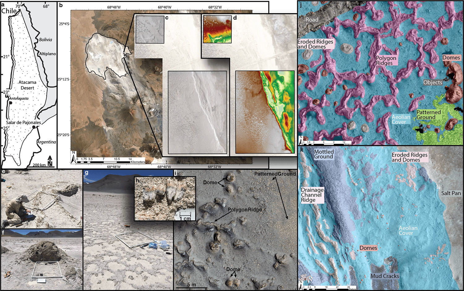
Fig. 1 Overview of Salar de Pajonales (SdP). A) Location of SdP within the Chilean Atacama Desert. B) Outline of SdP, note volcano to its south. C+D) Orthophotomosaic and DEM of the Dome Field generated with drone-collected images. E, F, G) Ridge, Dome, and Patterned Ground (biological soil crust) habitast at SdP, respectively. H) Pink and green horizons show endolithic microbial communities. I) Aerial view of Domes, Ridges, and Patterned Ground (biological soil crust) at SdP. J+K) Human-mapped ground truth classifications of the 12 feature classes in our study site.
Methods
We assessed the confidence with which habitats at SdP (polygon ridges, domes, and patterned ground) could be identified over a series of spatial resolutions with a methodology based on fully convolutional neural networks (FCNs, [13]). An FCN is a convolutional neural network with at least one fully-connected layer that adapts it to the semantic segmentation task. A “Confidence Score” was formulated to represent the degree to which one should trust FCN predictions [8]. The Confidence Score takes into account the correct and incorrect predictions made by the network, as well as the certainty (calculated using the Monte-Carlo Dropout method, [14]) associated with each prediction. BF-Score, precision, and recall were also calculated.
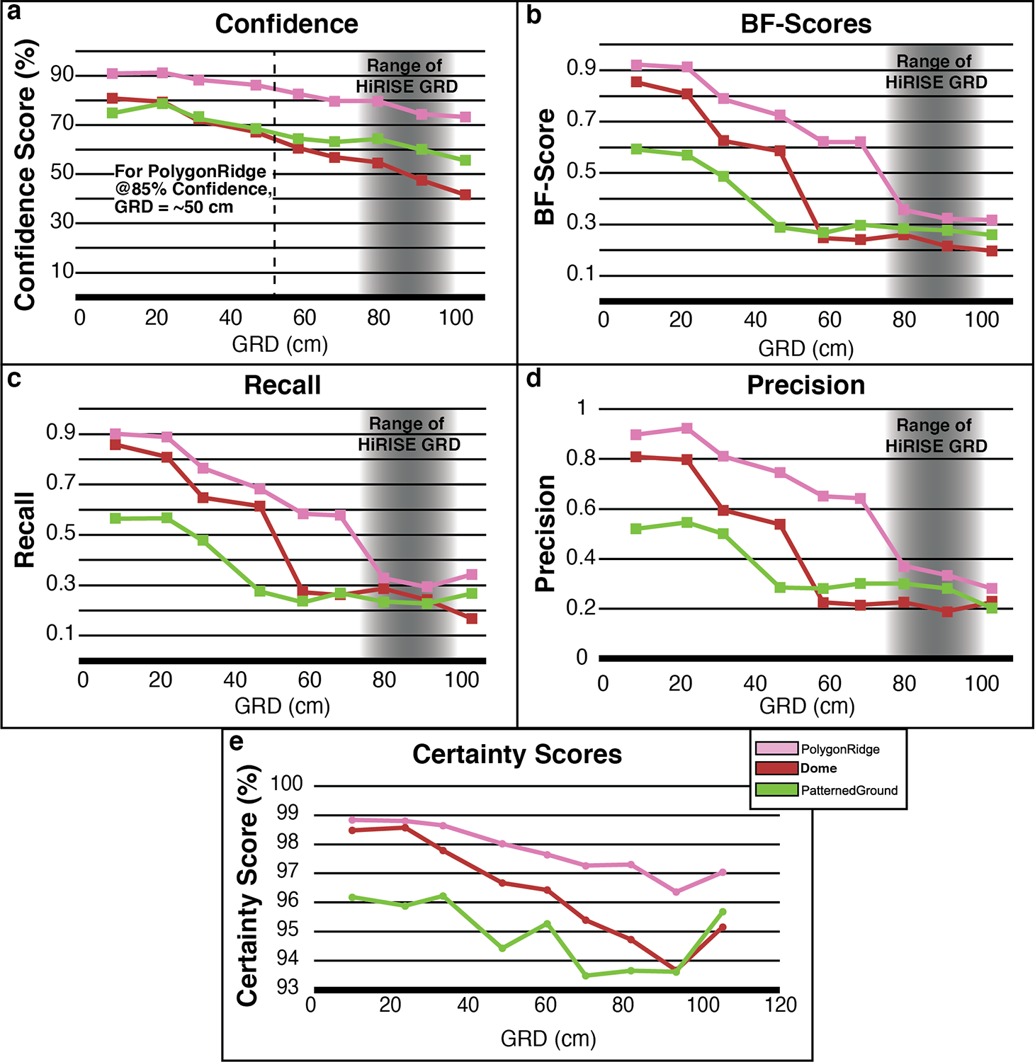
Fig. 2 Results as a function of Ground Resolved Distance (GRD). A) Confidence Score. B) BF-Score. C) Recall. D) Precision. E) Certainty. Gray region represents the approximate range of spatial resolutions achievable with HiRISE.
Results
The general characteristics of Precision, Recall, and BF-Score values as a function of image spatial resolution were relatively consistent between the habitats evaluated (Fig. 2b-d). We interpret the sharp drops in Precision, Recall, and BF-Score to mean that a spatial threshold critical for accurately segmenting (i.e., drawing a boundary around) a feature has been crossed. The threshold occurs at a GRD ~one-third the characteristic length scale of each feature, i.e., when the feature is spanned by 9 to 12 pixels. An analogy can be made to the Nyquist sampling frequency, wherein 2 to 3 pixels are required for a feature to be detected in an image. To achieve a 1-sigma level of identification confidence (Confidence Score ≥~85%) for the PolygonRidge class, a GRD approximately 20% its length scale is required, that is, it must be spanned by 15 to 20 pixels, or 5 to 10 times more pixels than is required to detect the feature. Conversely, Domes require a GRD ~6% their characteristic length scale (spanned by 50 to 65 pixels, or 17 to 33 times its detection limit) to be identified at the 1-sigma confidence level. PatternedGround could not be identified at the 1-sigma confidence level with the spatial resolutions studied here. This pattern suggests an intuitive hierarchy of recognition:
- detection: at 2-3 pixels, it is known that a feature exists
- segmentation: at 9-12 pixels, a boundary can be drawn around the feature
- identification: at ≥ 15 pixels, a class name can be accurately assigned to the feature.
These results emphasize the complexity and feature-specific nature of establishing identification thresholds in spatial resolution, and show that assuming the identifiability of a feature based only on its size may lead to overconfidence in the ability to identify it (e.g., the Dome class).Extending this work to establish the most- and least-identifiable habitats within presently-available images of Mars would be key for triaging habitats into a prioritized list of astrobiology targets and for informing future instrument specification requirements.
References:
[1] A. F. Davila et al., 2008. doi: 10.1029/2007JG000561.
[2] N. W. Hinman et al., 2022, https://www.frontiersin.org/article/10.3389/fspas.2021.797591
[3] R. E. Summons et al., Astrobiology, vol. 11, no. 2. p. 157, 2011.
[4] D. C. Fernández‐Remolar et al., 2013. doi: 10.1002/jgrg.20059.
[5] M. M. Osterloo et al., 2008. doi: 10.1126/science.1150690.
[6] T. D. Glotch, et al., 2016. doi: 10.1002/2015JE004921.
[7] E. K. Leask and B. L. Ehlmann, 2022, doi: 10.1029/2021AV000534.
[8] M. S. Phillips et al., Astrobiology, in review.
[9] J. Houston and A. J. Hartley, 2003. doi: 10.1002/joc.938.
[10] D. Häder and N. A. Cabrol, 2020. doi: 10.1111/php.13276.
[11] C. Rodríguez-Albornoz, Thesis, Universidad Católica del Norte, 2018.
[12] K. Warren-Rhodes et al., Nature Astronomy. in review.
[13] E. Shelhamer, et al., arXiv:1605.06211. p. tran, 2016.
[14] Y. Gal and Z. Ghahramani, ArXiv, vol. abs/1506.02142. 2016.
[15] B. L. Carrier et al., 2020. doi: 10.1089/ast.2020.2237.
[16] B. L. Ehlmann et al., 2016. doi: 10.1002/2016JE005134.
[17] T. C. Onstott et al., 2019. doi: 10.1089/ast.2018.1960.
[18] L. Hays, “NASA Astrobiology Strategy.” 2015.
How to cite: Phillips, M.: What is that? Identification confidence of Mars analog habitats with Deep Learning, Europlanet Science Congress 2022, Granada, Spain, 18–23 Sep 2022, EPSC2022-1200, https://doi.org/10.5194/epsc2022-1200, 2022.
AMADEE-20 is the latest Mars Analog Mission of the Austrian Space Forum (OeWF), conducted in Israel in the Negev Desert and hosted by the Israel Space Agency.

The 40 km long and 11 km wide Ramon Crater is an erosive crater unveiling a geological window of different sedimentary and volcanic processes with formations of sandstone, shales at the crater base, and mostly limestone and dolomite by the crater wall and represents sediments of the Thetis paleo-ocean with several volcanic and plutonic episodes including paleo-volcanos and granites. This nascency is accompanied by a semi-arid climate with dry summer (June – September), mild winter (December- February), and sparse vegetation only growing on the high rim hillslope and wadis (dry streams). Therefore, the Ramon Crater (Maktesh Ramon) presents remarkable geologic and geomorphological structures comparable to the Red Planet. Hence, beyond traditional analog mission applications, such as equipment behavior and evolving the know-how on crew management, we had the opportunity to develop research methods to catalyse the visibility of planetary explorations and develop structures for life-detection systematics and geoscientific techniques.
Two main segments of the mission; the mission support center (MSC)- on Earth time- and the field crew- on Mars time- were emulating a planetary surface mission by keeping a 20min time delay (10 min per signal direction) to account for the average signal travel time between Earth and Mars. The MSC was staffed by a Flight Director, Biomedical Engineers, Earth Communicators, CONTACTS,Records Manager, Procedure monitoring, Human Factors, Remote Science Support, Flightplan Team, Ground Support & Security, Science Data Officer, and Media Communication. The field crew was divided into two elements; I) the flight crew (6 AAs) with the analog astronauts, who conducted the experiments, and ii) the on-site support team (12 crew members) who provided support without interfering with the experiments or interacting directly with the AAs. Thereby, also maintaining a secured parameter and safety infrastructure for the simulation All major workflows of the mission were defined via the OeWF Standard Operating Procedures.

The flight crew habitat was provided by the Israel Space Agency and D-Mars, based upon the foldable D-Mars station design, complemented with a new module comprised of a Command module, Engineering/Science compartment, Crew quarters, Storage space, Mess and Hygiene module.
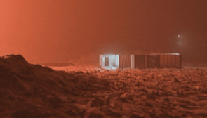
To provide a realistic platform for the experiments, isolation protocols were in place ensured. In total, 25 experiments were conducted from the fields such as engineering and robotics, human-robot interactions, health sciences, life sciences and geosciences. Outcomes of these experiments and the AMADEE-20 mission will be presented. This included an innovative science strategy, the exploration cascade which is an algorithm providing an efficient deployment sequence of scientific investigations (Groemer and Ozdemir, 2020).
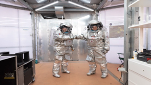
In the meantime, the preparations for the 14th analog mission of the OeWF, AMADEE-24 have started. With a comparable mission architecture as described above, we will be soliciting proposals for research experiments, to be selected peer-review process. These missions are a formidable platform for testing technologies, instruments and science workflows as well as it is a research opportunity for human factor studies.

REFERENCES:
Groemer G. and Ozdemir S. 2020. Planetary Analog Field Operations as a Learning Tool. Front. Astron. Space Sci. DOI: https://doi.org/10.3389/fspas.2020.00032
How to cite: Özdemir, S., Grömer, G., and Gruber, S.: Overview of AMADE-20 Mars Analog Mission and Insights from AMADEE-24, Europlanet Science Congress 2022, Granada, Spain, 18–23 Sep 2022, EPSC2022-1247, https://doi.org/10.5194/epsc2022-1247, 2022.
TP18 | Ionospheres of unmagnetized or weakly magnetized bodies
We estimate ion escape from Mars by combining observations and models. Assuming that upstream solar wind conditions are known, a computer model of the interaction between the solar wind and the planet is executed for different ionospheric ion production rates. This results in different amounts of mass loading of the solar wind. Then we obtain the ion escape rate from the model run that best fit observations of the bow shock location. This method enables studies of how escape depend on different parameters, and also escape rates during extreme solar wind conditions, applicable to studies of escape in the early solar system, and at exoplanets. This approach also allows us to use data sets traditionally not used for ion escape estimates, such as magnetic field and electron observations. We can also estimate the escape rate from a very small set of observations, during every orbit of a spacecraft around a planet or during one flyby of a planet.
How to cite: Holmstrom, M., Zhang, Q., Wang, X.-D., and Fatemi, S.: Estimations of Ion Escape from Mars, Europlanet Science Congress 2022, Granada, Spain, 18–23 Sep 2022, EPSC2022-239, https://doi.org/10.5194/epsc2022-239, 2022.
Unlike Earth, Venus doesn’t have an intrinsic magnetic field shielding it from the solar wind. However, an induced
magnetic field is generated from the interaction of solar wind and the dense atmosphere of the planet. Recent
Venus flybys by the BepiColombo mission in October 2020 and August 2021, and by Parker Solar Probe and Solar
Orbiter, are unique opportunities to further study the interaction between Venus and the Sun.
Observational data are essential in the study of this interaction but they are limited by the mission’s trajectory,
offering a constrained view of the processes that take place. On the other hand, simulations offer a global view
of the interactions, allowing us to get results with physical significance that would not have been possible from
observational data only. LatHyS is a three-dimensional parallel multi-species model using the hybrid formalism,
that represents the electrons as a massless fluid conserving the neutrality of the plasma, and the ions by numerical
macroparticles with variable weights. Ions and electrons are coupled together using the Maxwell equations, and the
macroscopic plasma parameters determine the evolution of the magnetic field (Ledvina et al. 2008). It was initially
developed at LATMOS, Paris, France, for Mars (Modolo et al. 2005) and later parallelized (Modolo et al. 2016) for
performance and optimization purposes. It has the advantage of having a self consistently calculated ionosphere.
LatHyS was recently adapted to the simulations of the interaction between the solar wind and Venus at IRAP,
Toulouse, France (Aizawa et al. 2022).
The work conducted aims at adapting a multi-grid method, initially adapted to LatHyS by Leclercq et al. 2016
for the study of Mars and Ganymede, to the case of Venus. The multi-grid refinement allows a more efficient use
of computing resources and an improved accuracy of the simulation thanks to a spatial resolution equivalent to or
lower than the ionospheric plasma scale height.
First, the multi-grid method is presented. Then, simulations using the multi-grid method on the solar wind’s
interaction with Venus are conducted, and their results are compared to simulations made using LatHyS with a
single homogeneous grid.
Finally the outputs of the numerical simulations are compared to data on the magnetic field and charged particles
from recent flybys and from the Venus Express mission, that orbited the planet from 2006 to 2014.
References:
Aizawa et al. 2022. https://doi.org/10.1016/j.pss.2022.105499
Leclercq et al. 2016. http://dx.doi.org/10.1016/j.jcp.2016.01.005
Ledvina et al. 2008. http://dx.doi.org/10.1007/s11214-008-9384-6
Modolo et al. 2005. https://doi.org/10.5194/angeo-23-433-2005
Modolo et al. 2016. http://dx.doi.org/10.1002/2015JA022324
How to cite: Jariel, E., Aizawa, S., Modolo, R., Leclercq, L., Baskevitch, C., Andre, N., and Persson, M.: Adapting a multi-grid method to a numerical simulation model of the interaction between Venus and the solar wind, Europlanet Science Congress 2022, Granada, Spain, 18–23 Sep 2022, EPSC2022-417, https://doi.org/10.5194/epsc2022-417, 2022.
Global dust storms at Mars engulf the entire planet in a dusty haze, causing increases in temperature and ion escape as dust is lifted up to 80 km in altitude. The two most recent storms occurred in 2007 (Mars Year (MY) 28) and 2018 (MY34), and have been observed by spacecrafts such as Mars Express (MEx). MEx has been operating at Mars since 2004, and has produced a long time-base of plasma measurements from as low as 250 km. Using MEx, we investigate whether the 2007 dust storm has influenced the magnetosphere of Mars by looking at the position of the bow shock and induced magnetospheric boundary, compared to the expected position provided by 3D magnetohydrodynamical models. To identify boundary positions, we use data from the ASPERA-3 instrument (Analyser of Space Plasma and EneRgetic Atoms) onboard MEx, which contains an electron spectrometer (ELS), ion mass analyser (IMA), neutral particle imager (NPI) and neutral particle detector (NPD). For this study, we use data from ELS and IMA. We consider a number of influences on the boundary position, including the solar wind conditions and the crustal fields. Our study period includes time before, during, and after the MY28 global storm, and we expected the bow shock and induced magnetospheric boundary to increase in altitude due to the storm. Out results show that the system is more complex, and multiple influences need to be distinguished to leave any change due to the dust storm itself.
How to cite: Regan, C., Coates, A., Wellbrock, A., Haythornthwaite, R., Jones, G., Sánchez-Cano, B., Holmström, M., Frahm, R., and Garnier, P.: Investigating the Global Dust Storm in Mars Year 28 with Mars Express, Europlanet Science Congress 2022, Granada, Spain, 18–23 Sep 2022, EPSC2022-527, https://doi.org/10.5194/epsc2022-527, 2022.
OPS1 | Ice Giant System Science and Exploration
The formation of giant planets can mainly be explained by two models: core accretion and gravitational collapse. Measurements of magnetic and gravity fields, as well as deep composition can help to constrain which scenario led to the formation of the Solar System Giant Planets. The deep composition also holds keys to understanding how primordial ices condensed and trapped the heavy elements, in the form of pure condensates, amorphous ices or clathrates. While the Galileo probe enabled measuring the abundances of noble gases and other heavy elements in Jupiter, the elemental composition of Saturn and the Ice Giants remains poorly constrained. Observations coupled with thermochemical modeling can help us to constrain the deep composition of giant planets and can also be used in synergy with mass spectrometry measurements of an in situ probe.
In this paper, we will present recent results of thermochemical modeling of the Ice Giants and compare them with results obtained for Jupiter.
How to cite: Cavalié, T., Lunine, J., Mousis, O., and Venot, O.: Observations and thermochemical modeling of gas and ice giant planets, Europlanet Science Congress 2022, Granada, Spain, 18–23 Sep 2022, EPSC2022-33, https://doi.org/10.5194/epsc2022-33, 2022.
Uranus’ atmosphere, once thought to be bland and static, has, in recent years, been shown to be anything but that. Radiative transfer retrieval analysis of high-resolution telescope observations has uncovered a dynamic atmosphere, displaying seasonal change and latitudinal variability. Uranus’ atmosphere is enshrouded in a global cloud/haze, meaning a robust aerosol layer model is required to probe any variability observed in its discrete features. One such example is its north polar hood, a bright ‘cap-like’ feature enshrouding the polar region northwards of ~45°N latitude (Fig. 1).

Figure 1: A false colour HST/WFC3 image of Uranus taken in 2018 displaying the north polar hood at the top right of the disc.
However, using remotely-sensed observations leads to a highly degenerate problem, resulting in competing aerosol models. Here we employ one such holistic aerosol model, derived by Prof. Patrick Irwin, in combination with the NEMESIS radiative transfer retrieval code. We utilise both space-based and ground-based observations to analyse the development of this hood over time, using the Minnaert approximation (Eqn. 1) to carry out a limb-darkening analysis of our observations to provide further constraint on our retrievals (demonstrated by Irwin et al., 2021).
I/F = (I/F)0μ0kµk-1 (1)
We demonstrate latitudinal variability in the methane volume mixing ratio via retrievals on HST/STIS and VLT/MUSE data. We then provide definitive evidence that a change in aerosol layers is a direct cause of brightening observed in the hood over time, and we display retrieval results on HST/WFC3 data spanning 2014 - 2021 to reveal what we find this change to be. This change is currently hypothesised as an increase in opacity of the middle (~1 - 2 bar) haze layer in the holistic model. These results strengthen the case for the holistic aerosol model and provide important context for the upcoming orbiter-probe mission to Uranus. Further scrutiny of this holistic aerosol model by employing it to the modelling of other discrete features will be valuable future work.
How to cite: James, A., Irwin, P., Dobinson, J., Wong, M., Simon, A., Karkoschka, E., Tomasko, M., and Sromovsky, L.: Variability in the Uranian atmosphere: Uranus' north polar hood, Europlanet Science Congress 2022, Granada, Spain, 18–23 Sep 2022, EPSC2022-87, https://doi.org/10.5194/epsc2022-87, 2022.
Introduction
Triton is the biggest satellite of Neptune. It was only visited by Voyager 2 in 1989. During this mission, the surface temperature was found to be only 38 K and the surface pressure 16 bar. It has a tenuous nitrogen atmosphere similar to the one of Pluto. This atmosphere was studied through stellar occultations and airglow observations, revealing traces of CH4 near the surface and also the presence of atomic nitrogen and hydrogen (Broadfoot et al. 1989). Radio observations pointed out the presence of a surprisingly dense ionosphere (Tyler and al. 1989). Strobel et al. (1990), Stevens et al. (1992) and Krasnopolsky and Cruikshank (1995) showed the consideration of electronic precipitation from Neptune’s magnetosphere was critical to explain the observed electronic number densities. At this distance from the Sun, the interplanetary radiation flux is also not negligible, particularly at Lyman- where it is comparable to the solar one (Broadfoot et al. 1989). Photochemical models of Triton’s atmosphere are few and were published following the Voyager flyby (Krasnopolsky et al. 1993, Krasnopolsky and Cruikshank 1995, Strobel and Summers 1995). Thus, we have developed a new photochemical model of this atmosphere with an up-to-date chemical scheme in order to prepare a potential mission to the Neptunian system.
The photochemical model and methodology
As the atmosphere of Triton is mostly N2 with traces of CH4, it recalls the one of Titan. Capitalizing on these similarities, we used a photochemical model of Titan’s atmosphere (Dobrijevic et al. 2016) with the chemical scheme of Hickson et al. (2020) and adapted it to Triton. To do this, we changed the critical input parameters, using data from Strobel and Zhu (2017), and updated the chemical scheme. This led us to add new atmospheric species and consider new chemical reactions. We also added the interplanetary flux and the precipitation of magnetospheric electrons. But as Triton’s atmospheric conditions are extreme, we expected large uncertainties on our results. Thus, we first computed the nominal composition of the atmosphere and then took into account the uncertainties on chemical reaction rates by using a Monte-Carlo procedure. These results were then treated through a sensitivity analysis to see how these uncertainties propagate in the model. We also added a water flux at the top of the atmosphere and used an electron transport code to better model the interaction between Triton and Neptune’s magnetosphere along its orbit.
Results
With the nominal results, we identify critical parameters having a significant influence on the results, such as the eddy diffusion coefficient, magnetospheric electrons or the solar flux. In addition, we highlight the main production and loss processes for the main atmospheric species. The two dominant processes are N2 ionization and dissociation by solar radiation and magnetospheric electrons, which influence the overall chemistry, and methane photolysis, that governs the chemistry in the lower atmosphere where the absorption of the Lyman- radiation is maximum. Nitrogen chemistry leads to the production of atomic nitrogen, N2+ and N+ that appear in several important reactions while methane photolysis is a source of H, H2, radicals and hydrocarbons. Due to the low temperature near the surface, these hydrocarbons condense and form hazes that were observed by Voyager.
The results of the Monte-Carlo procedure show that we have indeed large uncertainties for most of the main atmospheric species. We also observe epistemic bimodalities in the abundance distribution of some species. These uncertainties rise from the lack of knowledge about reaction rates at temperatures typical of Triton’s atmosphere, which leads to large uncertainty factors on reaction rates. With the sensitivity analysis, we identify key reactions that contribute the most to the model’s uncertainties. These reactions need to be studied in priority in order to decrease the uncertainties on the results and remove any epistemic bimodalities, thus improving the significance of photochemical results.
References
[1] Broadfoot, A. L., S. K. Atreya, J. L. Bertaux, J. E. Blamont, A. J. Dessler, et al. “Ultraviolet Spectrometer Observations of Neptune and Triton.” Science 246, no. 4936 (December 15, 1989): 1459–66. https://doi.org/10.1126/science.246.4936.1459.
[2] Tyler, G. L., D. N. Sweetnam, J. D. Anderson, S. E. Borutzki, J. K. Campbell, et al. “Voyager Radio Science Observations of Neptune and Triton.” Science 246, no. 4936 (December 15, 1989): 1466–73. https://doi.org/10.1126/science.246.4936.1466.
[3] Strobel, Darrell F., Andrew F. Cheng, Michael E. Summers, and Douglas J. Strickland. “Magnetospheric Interaction with Triton’s Ionosphere.” Geophysical Research Letters 17, no. 10 (1990): 1661–64. https://doi.org/10.1029/GL017i010p01661.
[4] Stevens, Michael H., Darrell F. Strobel, Michael E. Summers, and Roger V. Yelle. “On the Thermal Structure of Triton’s Thermosphere.” Geophysical Research Letters 19, no. 7 (April 3, 1992): 669–72. https://doi.org/10.1029/92GL00651.
[5] Krasnopolsky, Vladimir A., and Dale P. Cruikshank. “Photochemistry of Triton’s Atmosphere and Ionosphere.” Journal of Geophysical Research 100, no. E10 (1995): 21271. https://doi.org/10.1029/95JE01904.
[6] Krasnopolsky, V. A., B. R. Sandel, F. Herbert, and R. J. Vervack. “Temperature, N2, and N Density Profiles of Triton’s Atmosphere - Observations and Model.” Journal of Geophysical Research 98 (February 1, 1993): 3065–78. https://doi.org/10.1029/92JE02680.
How to cite: Benne, B., Dobrijevic, M., Cavalié, T., Loison, J.-C., and Hickson, K.: A photochemical model of Triton's atmosphere with an uncertainty propagation study, Europlanet Science Congress 2022, Granada, Spain, 18–23 Sep 2022, EPSC2022-139, https://doi.org/10.5194/epsc2022-139, 2022.
Introduction
To understand solar system formation it is critical to know how Uranus and Neptune formed. This requires knowledge of internal composition. Uranus and Neptune are generally referred to as ”ice-giants” in recent literature, as it has been inferred that their interiors are ice-dominated. Physical measurements from the Voyager 2 flybys include mass, radius, oblateness, low order gravity coefficients, moments of inertia, and magnetic field snapshots. One fundamental issue is that high temperature and pressure ice mixtures have similar densities to silicates mixed with hydrogen and helium. Therefore, existing physical constraints cannot by themselves distinguish between ice or rock-dominated interiors and almost any interior model fits the observations [5,10]. Measurements of atmospheric composition and temperature provide a possible complementary window into these planets’ interiors and may provide a way to break the degeneracy [12]. Here we consider the case for ice and rock-dominated interiors and attempt to propose a consistent explanation.
The case for Ice Giants
Internally-generated magnetic fields are observed at Uranus and Neptune [11]. Fields are highly non-dipolar, suggesting a shallow origin. Magnetic field generation requires conducting fluid and the conventional explanation is super-ionic water at high temperature and pressure, implying ice-dominated interiors.
Spectroscopic atmospheric CO observations provide further evidence favouring the ice giant model. CO has higher abundance in Uranus’ and Neptune’s stratospheres than in their tropospheres, indicating an external source [7]. Uranus has ~8 ppb stratospheric CO and <2 ppb tropospheric CO, which can mostly be accounted for with background interplanetary dust particle flux. Conversely, Neptune’s stratospheric CO abundance is the largest of any giant planet at ~1000 ppb. The only way to feasibly explain this is with a kilometre-scale ancient comet impact and shock chemistry, where cometary water reacts with methane in Neptune’s atmosphere to form CO [7,9].
More relevant to the interior is that Neptune appears to have ~100 ppb tropospheric CO. Conventionally, this is explained by quenching CO dredged up from the deep interior by Neptune’s vigorous tropospheric mixing. Thermochemical models predict ~400 x O/H enrichment over solar abundance is required to reproduce this CO amount [2,8]. This extreme enrichment requires ~90% water ice in Neptune’s interior, again implying an ice-dominated interior. It is usually extrapolated that Uranus is also an ice giant with a similarly extreme oxygen and ice abundance, where the lack of CO in Uranus’ troposphere is conveniently explained by more sluggish tropospheric mixing.
Issues with the Ice Giant model
Although ice-dominated interiors can explain many observational aspects of Uranus and Neptune, there are also some worrying discrepancies.
1) Most icy bodies in the outer solar system have rock fractions of ~70%. If Uranus and Neptune formed from similar objects, then we require some explanation of where the missing rock fraction has gone or why the planetesimals that formed Uranus and Neptune are different to anything we observe today.
2) Measurements of atmospheric methane on Uranus and Neptune suggest deep abundances of a few percent [6]. This implies a C/H enrichment of ~50–100 x solar [1], which is much lower than that inferred for O/H from tropospheric CO.
3) D/H is ~4x10⁻⁵ on both Uranus and Neptune [3]. This is much lower than D/H observed in modern solar system icy objects such as comets, which typically have D/H ∼15–60x10-5. If interiors of Uranus and Neptune are well mixed and equilibrated, this implies only ~15% of the interiors can be ice, suggesting ~50–100 x solar enrichment [12]. Again, much lower than inferred from CO. A way around this is for interiors to only be partially mixed and equilibrated, with more D hiding in the unobservable deep atmosphere. Alternatively, some form of extinct exotic ices with lower D/H could be the source material.
In summary, exotic ices, incomplete interior mixing, and unusually ice-rich planetesimals have all been invoked to make atmospheric observation consistent with the ice giant model. Not impossible, but also not entirely convincing as an explanation.
Rock Giant interiors as a potential solution
The alternative is that Uranus and Neptune’s interiors are rock-dominated. In this case we need to explain magnetic field generation and Neptune’s tropospheric CO.
Recent work shows mixtures of silicates, hydrogen, and helium may be conductive at relevant pressures and temperatures, so super-ionic water is not necessarily required to generate magnetic fields [4]. Alternatively, there is no-doubt some ice in Uranus and Neptune’s interiors, which may form thin shell dynamos and explain non-dipolar field structures.
Recent work also shows tropospheric CO may not actually be present throughout the troposphere and may be limited to the upper troposphere [12,13]. In this case, CO could be entirely sourced externally from comets.
Profiles with CO limited to pressures <1 bar can fit spectroscopic observations very well, but require reduced upper troposphere eddy mixing to allow CO to survive long enough post-comet-impact to still be observable today. This seems plausible, as inspection of the Voyager 2 temperature profile and lapse rate suggest the upper troposphere is relatively stable [12]. Furthermore, Far-IR brightness temperatures suggest the boundary between radiative and convective zones may be ~1 bar.
Conclusion
Recent advances in our understanding of CO profiles on Neptune and high-pressure conductivity of silicate/hydrogen/helium mixtures suggests that rock-dominated interiors for Uranus and Neptune are becoming more plausible than conventional ice giant scenarios. Such a rock giant could be formed from planetesimals with similar rock:ice ratios and D/H ratios to modern-day outer solar system comets, Kuiper belt objects, and icy moons. Interiors could also be well mixed and equilibrated. This opens the possibility of simpler formation mechanisms for Uranus and Neptune, with both planets forming in similar ways, and avoiding any requirements for dubious ice compositions.
References
[1] Atreya+ 2020. https://ui.adsabs.harvard.edu/abs/2020SSRv..216...18A/abstract
[2] Cavalié+ 2017. https://ui.adsabs.harvard.edu/abs/2017Icar..291....1C/abstract
[3] Feuchtgruber+ 2013. https://ui.adsabs.harvard.edu/abs/2013A%26A...551A.126F/abstract
[4] Gao+ 2022. https://ui.adsabs.harvard.edu/abs/2022PhRvL.128c5702G/abstract
[5] Helled+ 2020. https://ui.adsabs.harvard.edu/abs/2020RSPTA.37890474H/abstract
[6] Irwin+ 2019. https://ui.adsabs.harvard.edu/abs/2019Icar..331...69I/abstract
[7] Lellouch+ 2005. https://ui.adsabs.harvard.edu/abs/2005A%26A...430L..37L/abstract
[8] Luszcz-Cook+de Pater 2013. https://ui.adsabs.harvard.edu/abs/2013Icar..222..379L/abstract
[9] Moreno+ 2017. https://ui.adsabs.harvard.edu/abs/2017A%26A...608L...5M/abstract
[10] Neuenschwander+Helled 2022. https://ui.adsabs.harvard.edu/abs/2022MNRAS.512.3124N/abstract
[11] Soderlund+Stanley 2020. https://ui.adsabs.harvard.edu/abs/2020RSPTA.37890479S/abstract
[12] Teanby+ 2020. https://ui.adsabs.harvard.edu/abs/2020RSPTA.37890489T/abstract
[13] Teanby+ 2019. https://ui.adsabs.harvard.edu/abs/2019Icar..319...86T/abstract
How to cite: Teanby, N., Irwin, P., Wright, L., and Myhill, R.: Monsters of rock: are Uranus and Neptune rock giants?, Europlanet Science Congress 2022, Granada, Spain, 18–23 Sep 2022, EPSC2022-166, https://doi.org/10.5194/epsc2022-166, 2022.
Water vapour in the stratospheres of Uranus and Neptune has previously been shown to originate from external sources. These sources could include comet impacts [4], interplanetary dust particles [8], or rings and moons [1]. Stratospheric water was first detected on Uranus and Neptune by the Short-Wavelength Spectrometer (SWS) on the Infrared Space Observatory (ISO) [2], but the uncertainties were relatively large due to lack of constraint on the vertical water profiles and relatively low spectral resolution of the observations.
Here we present new observational constraints on Uranus’ and Neptune’s externally sourced stratospheric water abundance using disc-averaged high spectral resolution observations of the 557 GHz water emission line from Herschel’s Heterodyne Instrument for the Far-Infrared (HIFI). On both planets the emission line is significantly broadened by disc-averaging of Doppler shifts from planetary rotation, which was carefully accounted for in our analysis [10]. Derived stratospheric column water abundances are 0.56+0.26-0.06 x 1014 cm-2 for Uranus and 1.9+0.2-0.3 x 1014 cm-2 for Neptune. These results imply Neptune has about four times as much stratospheric water as Uranus, and are consistent with previous determinations from ISO-SWS and Herschel-PACS, but with improved precision.
For Uranus excellent observational fits are obtained by scaling photochemical model profiles [3,7] or with step-type profiles with water vapor limited to <=0.6mbar. However, Uranus’ cold stratospheric temperatures imply a ~0.03mbar condensation level, which further limits water vapor to pressures <=0.03 mbar. Neptune’s warmer stratosphere has a deeper ~1 mbar condensation level, so emission-line pressure broadening can be used to further constrain the water profile. For Neptune, excellent fits are obtained using step-type profiles with cutoffs of ~0.3-0.6 mbar or by scaling a photochemical model profile [7]. Step-type profiles with cutoffs >=1.0 mbar or <=0.1 mbar can be rejected with 4σ significance. Rescaling photochemical model profiles from [7] to match our observed column abundances implies similar external water fluxes for both planets: 8.3+4.0-0.9 x 104 cm-2s-1 for Uranus and 12.7+1.3-2.0 x 104 cm-2s-1 for Neptune.
This inferred water influx rates suggest that Uranus and Neptune may in fact have very similar IDP fluxes, unless there are significant water-loss processes that are not accounted for in current photochemical models [3,7]. This is unexpected as the IDP flux on Neptune is expected to be higher due to its closer proximity to the Kuiper belt. For example, the dynamical model of [8] predicts that the flux of IDP grains is around seven times higher on Neptune than on Uranus, but model uncertainties are large enough so as not to preclude a similar flux. The comet impact rates on Uranus and Neptune are also predicted to be quite similar [5,11], so both planets may experience similar external flux processes.
Our new analysis suggests that Neptune’s approximately four times greater observed water column abundance is primarily caused by its warmer stratosphere preventing loss by condensation, rather than by a significantly more intense external source. Larger error bars on the Uranus estimates are due to greater uncertainty in the high-altitude temperature profile. To reconcile these water fluxes with other observed stratospheric oxygen species (CO and CO2) requires either a significant CO component in interplanetary dust particles (Uranus) or contributions from cometary impacts (Uranus, Neptune). In particular, the large CO abundance in Neptune’s stratosphere suggests that we just happen to be observing Neptune at a time shortly after a large comet impact [4,6,9].
Further details of our results and analysis are available in our recent publication [10].

Fig1: Herschel-HIFI line-to-continuum ratio spectra of the 557GHz water line for HRS and WBS spectrometers. The water line is clearly visible at high signal to noise on both planets, but the line is broadened due to Doppler shift combined with the disc-broadened nature of the HIFI spectra. (Figure from https://doi.org/10.3847/PSJ/ac650f, see reference [10]).
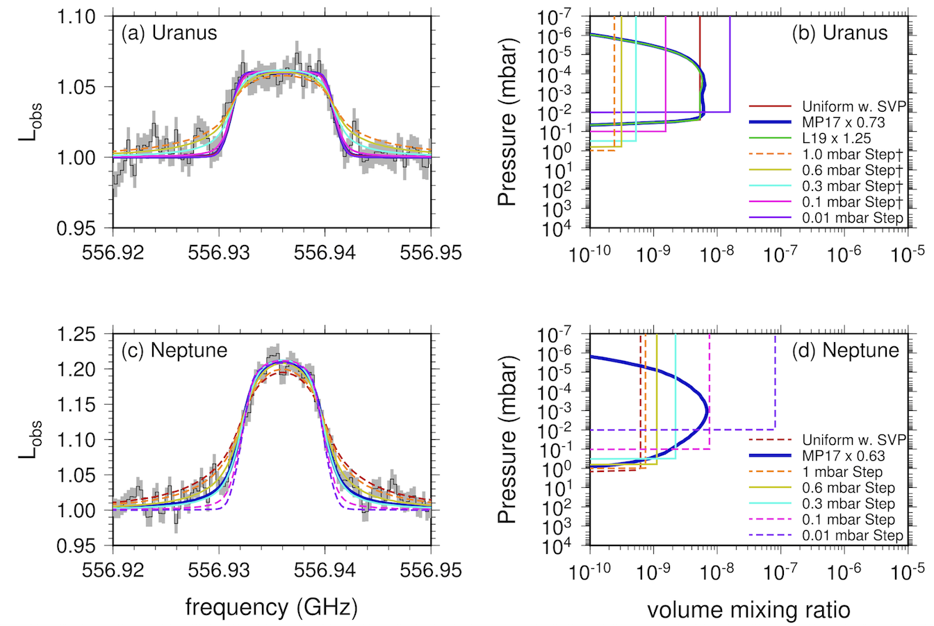
Fig2: Fits to Uranus and Neptune HIFI-HRS spectra 557GHz water line. (a,b) Uranus can be fitted with step profiles with a step pressure less than ~0.6mbar or by scaling photochemical profiles. However, significant water vapour is unlikely at pressures above ~0.03mbar due to saturation. (c,d) Neptune can be fitted with step profiles with a step in the pressure range 0.3-0.6mbar or by scaling photochemical profiles. (Figure from https://doi.org/10.3847/PSJ/ac650f, see reference [10]).
References
[1] Cavalié+ 2019. https://ui.adsabs.harvard.edu/abs/2019A%26A...630A..87C/abstract
[2] Feuchtgruber+ 1997. https://ui.adsabs.harvard.edu/abs/1997Natur.389..159F/abstract
[3] Lara+ 2019. https://ui.adsabs.harvard.edu/abs/2019A%26A...621A.129L/abstract
[4] Lellouch+ 2005. https://ui.adsabs.harvard.edu/abs/2005A%26A...430L..37L/abstract
[5] Levison 2000. https://ui.adsabs.harvard.edu/abs/2000Icar..143..415L/abstract
[6] Moreno+ 2017. https://ui.adsabs.harvard.edu/abs/2017A%26A...608L...5M/abstract
[7] Moses+Poppe 2017. https://ui.adsabs.harvard.edu/abs/2017Icar..297...33M/abstract
[8] Poppe 2016. https://ui.adsabs.harvard.edu/abs/2016Icar..264..369P/abstract
[9] Teanby+ 2019. https://ui.adsabs.harvard.edu/abs/2019Icar..319...86T/abstract
[10] Teanby+ 2022. https://ui.adsabs.harvard.edu/abs/2022PSJ.....3...96T/abstract
[11] Zahnle 2003. https://ui.adsabs.harvard.edu/abs/2003Icar..163..263Z/abstract
How to cite: Teanby, N., Irwin, P., Nixon, C., Cordiner, M., and Wright, L.: Uranus and Neptune's stratospheric water abundance and external flux from Herschel-HIFI, Europlanet Science Congress 2022, Granada, Spain, 18–23 Sep 2022, EPSC2022-168, https://doi.org/10.5194/epsc2022-168, 2022.
The past year has seen many papers underlining the significance of a space mission to Uranus and Neptune. Proposed mission plans usually involve a ~10 year cruise time to the ice giants. This cruise time can be utilized to search for low-frequency gravitational waves (GWs) by observing the Doppler shift caused by them in the Earth-spacecraft radio link. We calculate the sensitivity of prospective ice giant missions to GWs in comparison to former planetary missions which searched for GWs. Then, adopting a steady-state black hole binary population, we derive a conservative estimate for the detection rate of extreme mass ratio inspirals (EMRIs), supermassive- (SMBH) and stellar mass binary black hole (sBBH) mergers. For a total of ten 40-day observations during the cruise of a single spacecraft, approximately 0.5 detections of SMBH mergers are likely, if Allan deviation of Cassini-era noise is improved by ~102 in the 10−5 − 10−3 Hz range. For EMRIs the number of detections lies between O(0.1) − O(100). Furthermore, ice giant missions combined with the Laser Interferometer Space Antenna (LISA) would improve the GW source localisation by an order of magnitude compared to LISA by itself. With a significant improvement in the total Allan deviation, a Doppler tracking experiment might become as capable as LISA at such low frequencies, and help bridge the gap between mHz detectors and Pulsar Timing Arrays. Thus, ice giant missions could play a critical role in expanding the horizon of gravitational wave searches and maybe even be the first to detect the first SMBH merger.
How to cite: Soyuer, D., Zwick, L., D'Orazio, D., and Saha, P.: Ice Giant Missions as Gravitational Wave Detectors, Europlanet Science Congress 2022, Granada, Spain, 18–23 Sep 2022, EPSC2022-207, https://doi.org/10.5194/epsc2022-207, 2022.
Past years have seen numerous papers underlining the importance of a space mission to the ice giants in the upcoming decade. Proposed missions to Uranus and Neptune usually involve a ~10 year cruise time to the ice giants. In this phase, the spacecraft trajectories will mainly be determined by the configuration of massive bodies in the solar system. Interplanetary trajectories are monitored by recording Doppler shifts in the time series of the radio link between Earth and the spacecraft. The presence of dark matter (DM) affects the trajectory by introducing a small radial acceleration, which in turn reduces the velocity of the spacecraft over years of interplanetary travel. Additionally, bounds on the precession rate of ice giants could help constrain the local DM density and potentially rule out modified gravity scenarios.
We investigate the possibility of detecting the gravitational influence of DM in the solar system on the trajectory of prospective Doppler ranging missions to Uranus and Neptune, and also estimate the constraints such a mission can provide on modified and massive gravity theories via extra-precession measurements using orbiters around the ice giants.
The precision of these measurements is limited by the noise on the the two-way frequency fluctuation of the Doppler link. For the trajectory deviations, we developed a numerical procedure for reconstructing the influence of DM in the Doppler signal of thousands of simulated ice giant missions.
The noise improvements required to guarantee a local detection of dark matter in the early 2040s are realistic, provided they become one of the priorities during mission development.
How to cite: Zwick, L., Soyuer, D., and Bucko, J.: Prospects for a local detection of dark matter with future missions to Uranus and Neptune, Europlanet Science Congress 2022, Granada, Spain, 18–23 Sep 2022, EPSC2022-226, https://doi.org/10.5194/epsc2022-226, 2022.
Atmospheric probes provide a critical method for understanding the Ice Giants, offering unique insight into atmospheric composition, structure, and dynamics. Such in situ measurements are vital to understanding the formation and evolution of these bodies and our solar system. To pursue these scientific opportunities space agencies are now turning their attention to the developmemnt of atmospheric probes to the Ice Giants and other bodies. The newly released Decadal Survey prioritized Uranus and Saturn probes as well as a Venus in situ explorer. Few such missions have flown and it is not likely that there will be other atmospheric entry probes until the DAVINCI+ Venus probe mission in the early 2030’s. Entry probe concepts such as these require a delicate balance between science objectives, orbital mechanics, atmospheres, and signal processing. The development of future entry probe missions will rely on tools which allow mission teams to concurrently filter and compare trajectories to optimize science return.
To aid science planning for future entry probe missions we have developed a tool for Visualization of the Impact of PRobe Entry (VIPRE) conditions on science, mission and spacecraft design. VIPRE provides concurrent design capabilities for entry probe and lander missions by combining a precomputed database of optimized interplanetary trajectories with analytical models for entry point targeting, atmospheric descent and data-return rates. The user is able to explore the science trade-space using a GUI to constrain a variety of entry, trajectory, and data sufficiency parameters. Constraint-based interaction allows for direct, easy evaluation of scientific value and mission feasibility in real time. VIPRE is flexible to a variety of mission architectures allowing direct comparison of mission value between combinations of orbiters, entry vehicles and landers.
Users primarily interact with VIPRE through a GUI. Figure 1 provides an illustration of some of the available mission design, science parameter and constraint intereractions within the VIPRE GUI. On its left edge, the GUI allows for the selection of a target body, Saturn in this case, and a range of filtering parameters. Based on these inputs, the GUI displays the top row of plots which indicate the filtered interplanetary trajectory parameters. Once a trajectory of interest is selected the “Overview” parameters are populated and the bottom row plots are generated to illustrate reachable probe entry locations, colored based on parameters of interest. Reachability, in this case, is defined by the selected filtering parameters as well as target specific constraints, i.e. avoiding Saturn’s rings. The GUI also allows for user definition of figures and filter parameters, shown in this example under the "Globe" and "Side by Side" tabs.
This talk presents the motivation and models used for the development of VIPRE. Applications to Uranus and Saturn probe missions are discussed. Of particular interest is the accessibility of high and low latitudes for probe entry, how this is influenced by mission architecture (flyby versus orbiting probe release), and data constraints due to probe communications geometry.
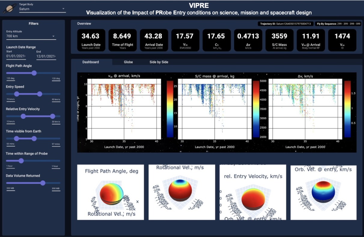
Figure 1. Example of VIPRE trajectory selection for a Saturn probe mission
[1] Probst, A. et al, VIPRE: A Tool Aiding the Design for Entry Probe Missions, The Planetary Science Journal 3.4 (2022) 98.
[2] Hofstadter, M. et al., Uranus and Neptune missions: A study in advance of the next planetary science decadal survey, Planetary and Space Science 177 (2019) 104680.
[3] National Academies of Sciences, Engineering, and Medicine. "Origins, Worlds, and Life: A Decadal Strategy for Planetary Science and Astrobiology 2023-2032." (2022).
How to cite: Davis, A., Landau, D., Atkinson, D., Hofstadter, M., Fedell, M., and Stonebreaker, R.: VIPRE: A Tool for Designing and Optimizing Science Return of Planetary Entry Probes, Europlanet Science Congress 2022, Granada, Spain, 18–23 Sep 2022, EPSC2022-262, https://doi.org/10.5194/epsc2022-262, 2022.
The ice giants Uranus and Neptune are the least understood class of planets in our solar system, while planets of their size, the most frequent among exoplanets, represent a common outcome of planet formation. Presumed to have a small rocky core, a deep interior comprising ~70% heavy elements surrounded by a more dilute outer envelope of H2 and He, Uranus and Neptune are fundamentally different from the better-explored gas giants Jupiter and Saturn. Because of the dearth of missions dedicated to their exploration, our knowledge of their composition and atmospheric processes is primarily derived from a single Voyager 2 flyby of each, complemented by subsequent remote sensing from Earth-based observatories, including space telescopes. As a result, Uranus's and Neptune's physical and atmospheric properties remain poorly constrained and their roles in the evolution of the Solar System are not well understood. Exploration of ice giant systems is therefore a high-priority science objective as these systems (which link together the magnetospheres, satellites, rings, atmosphere, and interior of these planets) challenge our understanding of planetary formation and evolution. In this context, the US planetary science decadal survey report recently recommended the launch of a flagship mission towards the Uranian system in the early 2030s. This mission would be composed of an orbiter aiming at exploring the Uranian system as a whole and a descent probe to directly sample the giant’s atmosphere.
Measurements to be made with a probe can be defined as Tier 1, representing threshold science required to justify the probe mission, and Tier 2 representing valuable science that significantly complement and enhance the threshold measurements, but of themselves are not sufficient to justify the mission. Tier 1 measurements comprise atmospheric noble gas abundances including helium, key noble gas isotope ratios, and the thermal structure of the atmosphere. Instrumentation required to achieve the Tier 1 measurements include a mass spectrometer, a helium abundance detector, and an atmospheric structure instrument comprising both sensors for pressure, temperature, a Tunable Laser System and atmospheric acoustic properties (speed of sound). Tier 1 science can be achieved with a probe making measurements near one to several bars. Tier 2 science includes measurements of key isotopic ratios, the abundances of atmospheric condensables and disequilibrium species, atmospheric dynamics, the net radiative flux transfer profile of the atmosphere, and the location, composition, properties, and structure of the clouds. To achieve all the Tier 2 science objectives requires a probe descending through at least ten bars carrying the full Tier 1 suite of instruments as well as a nephelometer, net flux radiometer, and an ultrastable oscillator to enable Doppler wind tracking of the probe throughout descent.
How to cite: Mousis, O. and Atkinson, D. H. and the Ice Giants team: Reference Science Payload for an Uranus Entry Probe, Europlanet Science Congress 2022, Granada, Spain, 18–23 Sep 2022, EPSC2022-572, https://doi.org/10.5194/epsc2022-572, 2022.
Background: The atmospheres of Uranus and Neptune are the most poorly constrained fluid atmospheres in the solar system. The ice giants were only visited, briefly, by the Voyager 2 spacecraft in the late 1980s. At Uranus, the Voyager 2 UV stellar and solar occultations detected a warm stratosphere and extremely hot thermosphere [1, 2], far in excess of heating caused by solar irradiance alone [3, 4]. Furthermore, Uranus has far smaller internal energy production than the other giant planets [5, 6] as well as a surprisingly well-equilibrated stratosphere given its 98º obliquity [7]. As the energy balance of Uranus’ atmosphere is unknown, it is often called the “Giant Planet Energy Crisis.”
Motivation and Aims: Between 1977 and 1998, dozens of stellar occultations by Uranus were observed from Earth (see [8] and references therein). In an Earth-based stellar occultation, stellar flux is diminished by differential refraction through the occulting atmosphere and is observed as a light curve. The original analyses of these light curves found cooler stratospheric and lower thermospheric temperatures than Voyager 2. Figure 1 shows the tension between the Earth-based and Voyager measurements of the upper atmosphere of Uranus. It is now possible to reprocess these archival light curves using modern techniques and better compare them to the Voyager 2 temperature profiles.
Methods: To reprocess the Earth-based stellar occultation light curves, we use a two-part procedure. We first fit the light curve to a smooth atmospheric model with power law temperature gradient [9] to set a boundary condition. We next perform inversion, which assumes ray optics, small bending angles, hydrostatic equilibrium, and an ideal gas to solve for temperature, pressure, and number density at each flux measurement [10]. This procedure has been significantly improved since the original data were published, allowing for non-isothermal boundary conditions, accurate uncertainties on output quantities, and much higher vertical resolutions [11].
In addition to producing atmospheric profiles from observed occultation light curves, we do the reverse by simulating Earth-based stellar occultation light curves using the Uranian temperatures reported by Voyager 2 [12]. We can then compare the generated light curves directly to our suite of observed ones.
Results: We present the temperature-pressure profiles from reanalysis of many archival Earth-based occultations and compare them to the published Voyager 2 findings. Further, we present the comparison of our synthetic Earth-based light curves, generated from a forward model of the Voyager 2 temperatures, to the observed Earth-based light curves. We comment on how consistent the Voyager 2 UV occultation findings are with Earth-based stellar occultation observations. Finally, we offer a revised Uranus temperature-pressure profile for the stratosphere and lower thermosphere based on these findings.
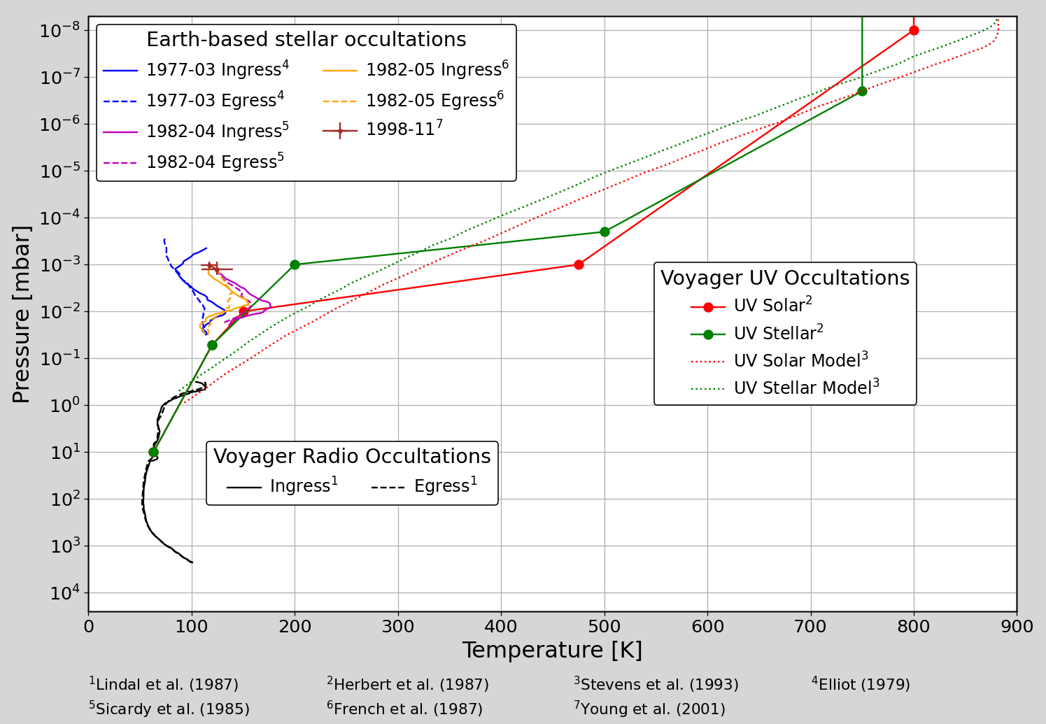
Figure 1. Comparison of remote sensing measurements of the atmosphere of Uranus. Earth-based occultations are blue [13], magenta [14], yellow [15] and brown [8]; Voyager UV occultations are solid red and green [1]; models are dotted red and green [2]; Voyager radio occultations are black [16]. Error bars are absent from this figure because they were not provided in the original publications.
References
[1] Herbert, F., et al. (1987). JGR, 92, pp. 15093–15109.
[2] Stevens, M. H., et al. (1993). Icarus, 101, pp. 45–63.
[3] Marley, M. S., and McKay, C. P. (1999). Icarus, 268-286.
[4] Li, C., Le, T., Zhang, X, and Yung, Y. (2018). J Quant Spectrosc Ra, 353–362.
[5] Pearl, J. C., Conrath, B. J., Hanel, R. A., Pirraglia, J. A, Coustenis, A. (1990). Icarus, 12-28.
[6] Bishop, J., et al. (1995). Neptune and Triton, pp. 427–487, University of Arizona Press.
[7] West, R. A., and Lane, A. L. (1987). JGR, 92, 30-36.
[8] Young, L. A., et al. (2001). Icarus, 153, pp. 236–247.
[9] Elliot , L. A., and Young, L. A. (1992). AJ, 991.
[10] Elliot, J. L., Person, M. J., & Qu, S. (2003). AJ, 126, 1041-1079.
[11] Saunders, W. R., Person, M. J., Withers, P. (2021). AJ, 161, 280.
[12] Chamberlain, D. and Elliot, J. (1997). PASP, 109, pp. 1170–1180.
[13] Elliot, J. L. (1979). Annu. Rev. Astron. Astrophys., 17, pp. 445-475.
[14] Sicardy, B., et al. (1985). Icarus, 64 pp.88-106.
[15] French, R. G., et al. (1987). Icarus, 69, pp. 499–505.
[16] Lindal, G. F. et al. (1987). JGR, 92, pp. 14987–15001.
How to cite: Saunders, W., Person, M., Withers, P., and French, R.: Uranus Upper-Atmospheric Temperatures From Stellar Occultations, Europlanet Science Congress 2022, Granada, Spain, 18–23 Sep 2022, EPSC2022-758, https://doi.org/10.5194/epsc2022-758, 2022.
Introduction
Our team has collected a 40+ year record of ground-based radio observations of Uranus, which constrain atmospheric circulation and chemistry in the 1 to 100 bar pressure region as a function of latitude, altitude, and season.
The Data Set
Our primary data set is 25 images of Uranus made at the Very Large Array (VLA) and Submillimeter Array (SMA) radio observatories between 1981 and 2022 (Fig. 1). Observations were made at wavelengths between 0.1 and 21 cm. They are augmented by unresolved measurements at wavelengths from 350 µm to 1.3 mm from the James Clerk Maxell Telescope (JCMT) and the Caltech Submillimeter Observatory (CSO).

Figure 1: VLA image of Uranus at a wavelength of 1 cm, observed in 2012. The North Pole is on the right. Bright regions have a lower abundance of absorbing species.
Retrievals of Atmospheric Properties
The data set is primarily sensitive to the vertical profiles of H2S, NH3, and H2O between about 0.7 and 100 bars (Fig. 2). We considered three models to constrain their vertical profiles.
Chemical Equilibrium Model: The abundance of species deep in the troposphere is allowed to vary with latitude, but vertically they are assumed to condense out according to their saturation vapor pressures. The saturation vapor pressure is allowed to be modified by a relative humidity anywhere from 0 to 10.
Hadley-Type Model: Low latitudes are in chemical equilibrium and represent regions of upwelling (Fig. 3). High latitudes represent areas of subsidence where condensable species are depleted down to a depth which is varied to fit the data.
Juno-Type Model: Inspired by results from the Juno spacecraft at Jupiter [1], all opacity is represented by NH3 with three free parameters: upper and lower atmospheric mixing ratios, and the pressure at which the transition between ratios occurs.
For all models that fit the data, we find:
- Regions poleward of ±50˚ are depleted in condensables relative to lower latitudes by a factor of ~50, down to a depth of ~20 to ~50 bars.
- Regions between the equator and ±30˚ are richer in condensables. Equilibrium models require more H2S in these regions than NH3.
- Regions between 30˚ and 50˚ North and South are intermediate in their abundance of condensables.
- In the 1 to 5 bar region, relative humidities at low latitudes are ~1.4 and they are ~0 over the poles, and/or the meridional temperature variations of ~ 2 K observed near 800 mbar [2] extend to these depths.
- The abundance of condensables over a large altitude range varies by ~30% near latitudes of 0˚, ±20˚ and ±75˚.
- During mid-summer the pole to equator contrast decreases.
Many of the features reported above have been seen previously [e.g., 3, 4], though our analysis is unique in spanning a large altitude and time range.
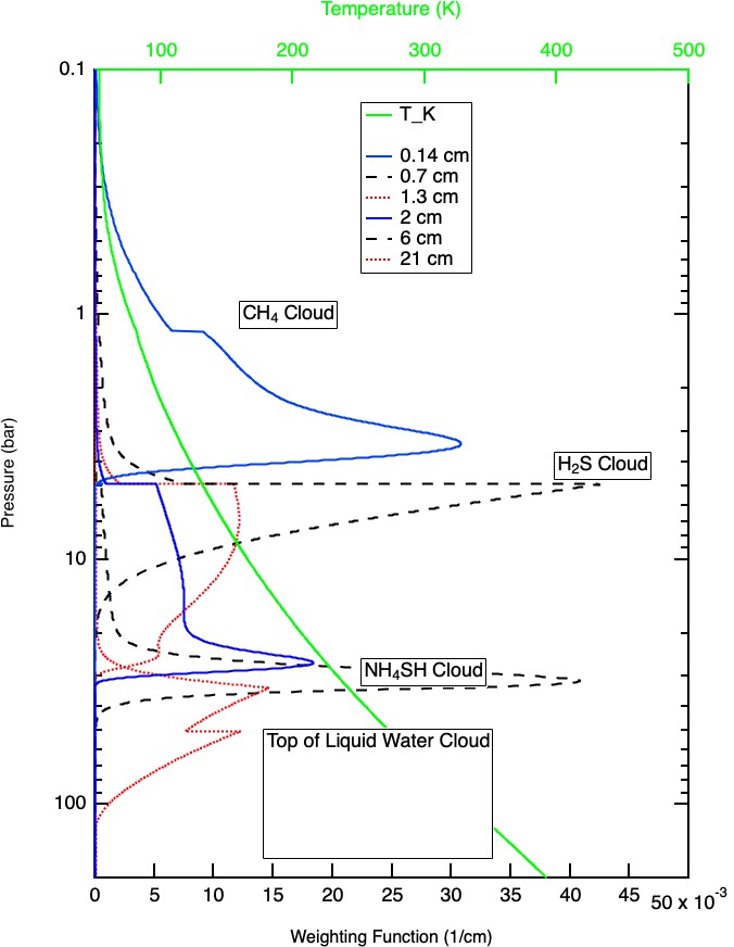
Figure 2: Weighting functions for the primary wavelengths used in this study, and the assumed atmospheric temperature profile. The location of various cloud layers is indicated.
Discussion
A large-scale circulation pattern is one possible cause of the observed spatial variations (Fig. 3). We refer to this as our Hadley-type model. (Uranus' poles receive more sunlight than the equator on an annual average, however, making this circulation opposite in a thermal sense to a classic Hadley cell.) At the time of the conference we expect to have completed dynamical modeling to test the plausibility of this scenario. In this model, smaller circulation patterns would explain the fainter banding seen in images (Fig. 1).
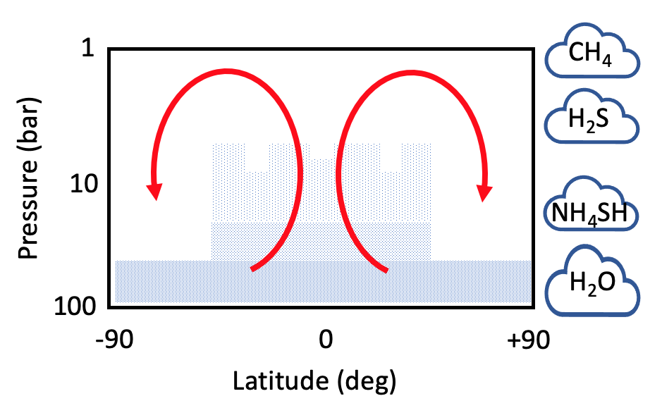
Figure 3: The density of blue dots is indicative of the observed absorber abundance. The altitude of expected clouds is shown along the right. A possible circulation pattern is indicated in red, with upwelling near the equator carrying absorber-rich air parcels upward. The rising air cools and clouds form, depleting air parcels in absorbers. Depleted air parcels then move poleward and descend at high latitudes.
An alternative explanation is what we refer to as a Juno-type model. The depletion of condensables in the ~5 to ~50 bar region of the Uranus atmosphere relative to deeper down and the meridional gradients are reminiscent of what the Juno spacecraft discovered at Jupiter [1]. Mechanisms proposed for Jupiter [e.g., 5] rely on vigorous convection. Since the variations at Uranus are more than 10x larger than those seen at Jupiter, but the uranian atmosphere near 1 bar seems less convectively active than Jupiter's, this interpretation would suggest that the deep Uranus troposphere is much more active than the upper troposphere. If such a process strongly depletes Uranus' 1 to 50 bar region of NH3 but depletes H2S to a lessor (but still significant) extent, that would explain why the observed absolute abundances of NH3 and H2S at Uranus are so much smaller than expected from planetary formation models, while the observed S/N ratio is much larger than expected [6].
The large-scale pole-to-equator brightness gradient and smaller-scale banding are always present in the spring, summer, and fall (the winter hemisphere cannot be seen from the Earth). For roughly ±5 years around the previous summer solstice (which occurred in 1985), however, the contrast between pole and equator was less than it was at other times, indicative of a weakening in circulation patterns. The next summer solstice is in 2028, so if we have indeed observed a seasonal effect, it should arise again in the next few years.
Acknowledgements
We thank the staff and funding agencies of the VLA, SMA, JCMT, and CSO observatories. We also thank Dr. Göran Sandell for providing the JCMT and CSO data used, and Dr.'s I. de Pater and E. Molter for useful discussions. Parts of this work were carried out at JPL/Caltech, under a contract with NASA.
References
[1] Bolton, S.J. et al. (2017) Science, 356, 6340/821. [2] Hanel, R.B. et al. (1986) Science, 233, 70–74. [3] Hofstadter, M.D. and Butler, B.J. (2003) Icarus, 165, 168–180. [4] Molter, E.M, et al. (2021) Plan. Sci Journ. 2:3. [5] Guillot, T. et al. (2020) JGR Planets, 125, e2020JE006403. [6] Atreya, S.K. et al. (2020) Space Sci Rev, 216:18.
How to cite: Hofstadter, M., Butler, B., Akins, A., Gurwell, M., and Friedson, J.: Radio Observations of Uranus: Implications for the Structure and Dynamics of the Deep Troposphere, Europlanet Science Congress 2022, Granada, Spain, 18–23 Sep 2022, EPSC2022-771, https://doi.org/10.5194/epsc2022-771, 2022.
How volatiles were incorporated in the building blocks of planets and small bodies in the protosolar nebula (PSN) remains an outstanding question. Some scenarios consider that planetesimals formed from a mixture of refractory material and volatiles trapped in amorphous ice in the outer nebula, while others hypothesize that volatiles have been incorporated in clathrates or formed pure condensates [1,2]. Here, we study the evolution of volatiles species in the PSN (H2O, CO, CO2, CH4, H2S, N2, NH3, Ar, Kr, Xe and PH3) considering two possible volatiles reservoir in the initial state: amorphous ice (see Figure 1) or pure condensates (see Figure 2). To do so, we use a 1D disk accretion model [3] with radial transport of trace species to compute the radial distribution of volatiles in the PSN. This model includes condensation/sublimation rates of pure condensates, as well as clathration/release rates when enough crystalline water is available. Figure 1 represents the case where volatiles are initially delivered to the PSN in the form of pure condensates. Figure 2 represents the case where volatiles are delivered to the PSN by amorphous ice. Species are released when amorphous grains cross the ACTZ region. Once delivered to the disk, the phase (solid or gaseous) of each species is ruled by the positions of its corresponding condensation and clathration lines. Clathration lines of the considered volatiles are closer to the Sun than their respective condensation lines, except for CO wich have its clathration line further from the sun than its condensation line. Gaseous volatiles condense or become entrapped (depending on the availability of water ice) when diffusing outward the locations of their lines. Conversely, volatiles condensed/entrapped in grains or pebbles are released in gaseous forms when drifting inward their lines. Peaks of abundances form close to each line. Our simulations show that a significant fraction of volatiles can be trapped in clathrates, only if they have initially been delivered in pure condensate forms to the disk. We also show that several regions in the protosolar nebula share a metallicity that is consistent with those measured in the atmospheres of the ice giants [3,4]. These findings have important implications for the formation history of the outer planets
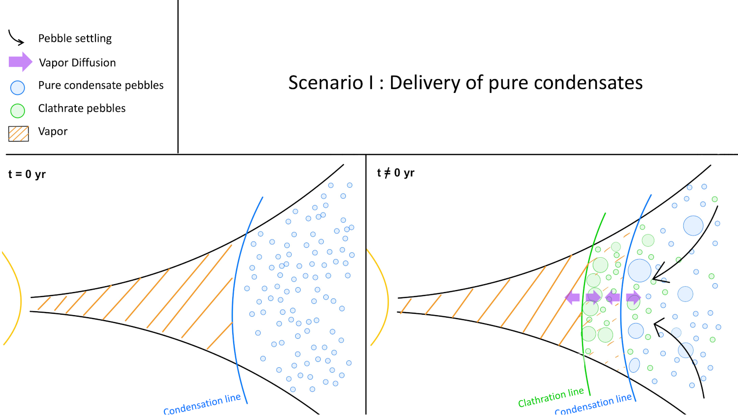
Figure 1 : Scheme showing the disk at initialization and at a given time. The volatiles are initially delivered under pure condensates and vapor. The vapor will condensate into clathrate hydrate, if there is enough crystalline water available. Grains drift inward while vapor undergo diffusion inward and outward. Leading to an accumulation of species at the place of condensation lines.
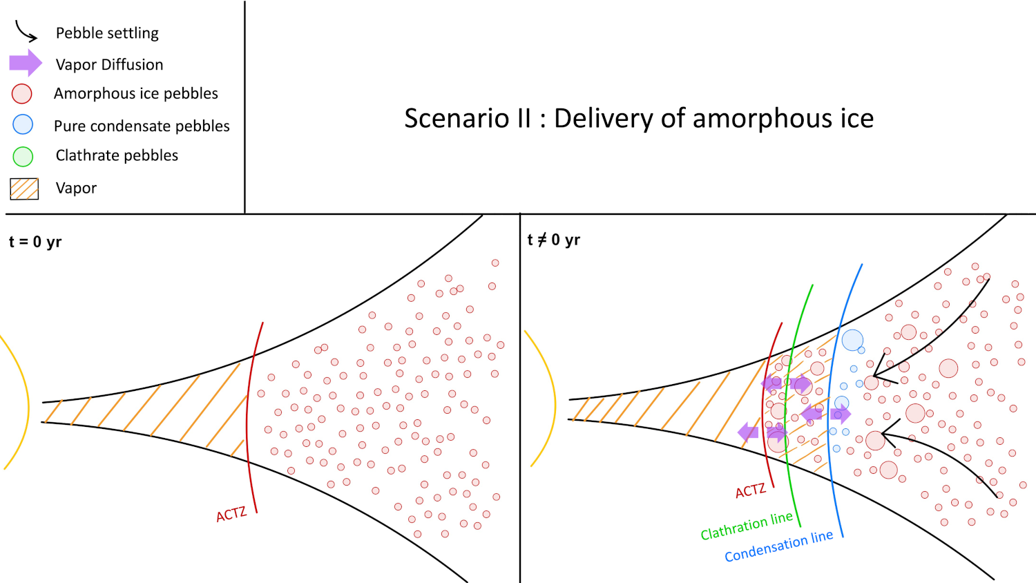
Figure 2 Scheme showing the disk at initialization and at a given time. The volatiles are initially delivered trapped into amorphous ice and vapor released from amorphous ice at the Amorphous to Crystalline Transition Zone (ACTZ). The clathration line is further than the ACTZ, since there no crystalline water after the ACTZ, clathration cannot happen, or is marginal if the clathration line is close to the ACTZ.
[1] : Gautier, D., Hersant, F., Mousis, O., et al. 2001, ApJL, 550, L227
[2] : Mousis, O., Ronnet, T., & Lunine, J. I. 2019, ApJ, 875, 9.
[3] : Aguichine, A., Mousis, O., Devouard, B., et al. 2020, ApJ, 901, 97.
[4] : Asplund, M., Grevesse, N., Sauval, A. J., et al. 2009, ARA&A, 47, 481.
[5] : Irwin, P. G. J., Toledo, D., Garland, R., et al. 2018, Nature Astronomy, 2, 420.
How to cite: Schneeberger, A., Mousis, O., Aguichine, A., and Lunine, J.: Evolution of the reservoir of volatiles in the protosolar nebula, Europlanet Science Congress 2022, Granada, Spain, 18–23 Sep 2022, EPSC2022-881, https://doi.org/10.5194/epsc2022-881, 2022.
Neptune's incomplete ring arcs have been stable since their discovery in 1984 by stellar occultation. Although these structures should be destroyed within a few months through differential Keplerian motion, imaging data over the past couple of decades have shown that these structures remain stable.
We present the first SPHERE near-infrared observations of Neptune's ring arcs taken at 2.2 μm (broadband Ks) with the IRDIS camera at the Very Large Telescope (VLT) in August 2016.
We derive accurate mean motion values for the arcs and the nearby satellite Galatea. The trailing arcs Fraternité and Égalité have been stable since they were last observed at VLT in 2007 (cf. Fig 1 left). Furthermore, we confirm the fading away of the leading arcs Courage and Liberté. Finally, we confirm the mismatch between the arcs' position and the 42:43 inclined and eccentric corotation resonances with Galatea, thus demonstrating that no 42:43 corotation model works to explain the azimuthal confinement of the arcs' material (cf. Fig. 1 right).
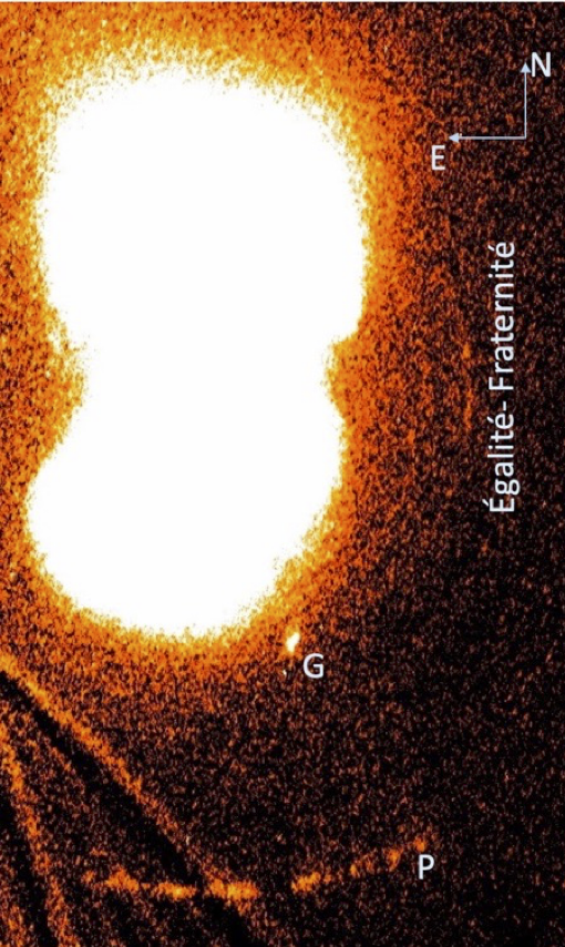
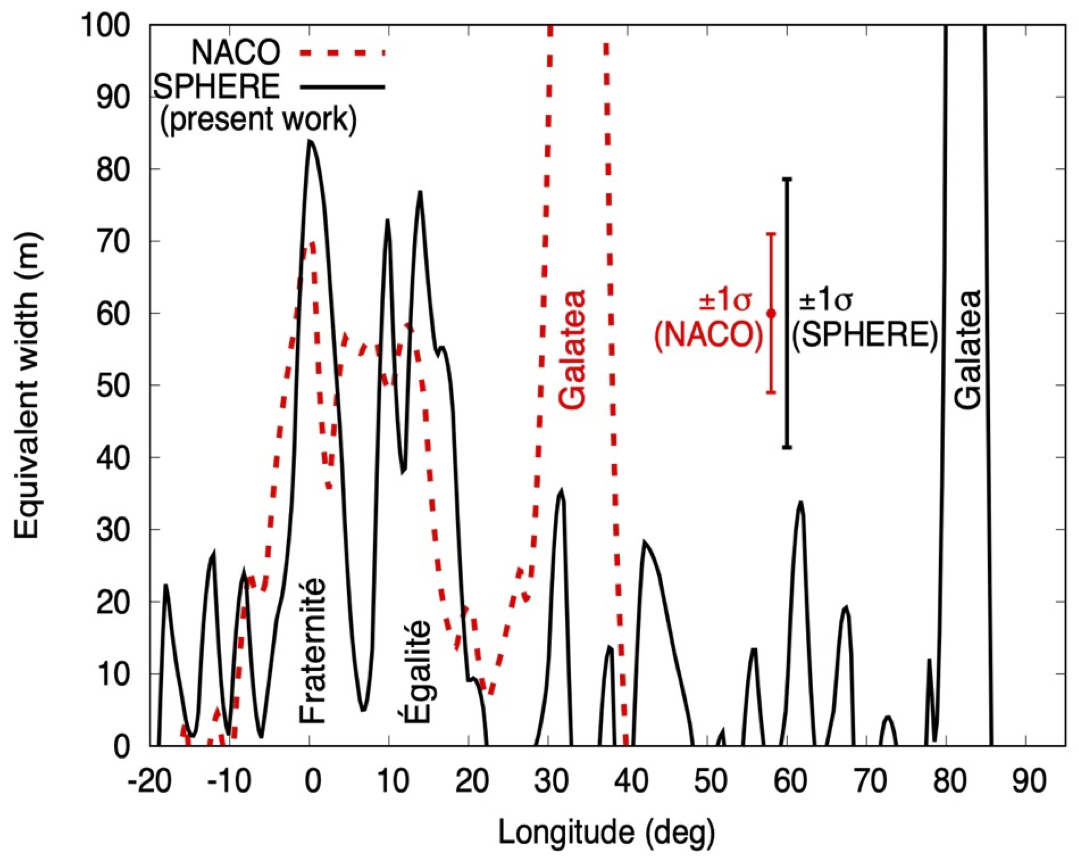
Fig. 1 (left) 68 projected and co-added images of Neptune’s equatorial plane, revealing material along the arcs Fraternité and Égalité, as well as the satellites Proteus (P) and Galatea (G). The frame is 7.1x10.7 arcsec2 wide. (right) Equivalent width of the arcs (Fraternité and Égalité), at an angular resolution of 2°. The X-axis origin is the longitude LFr of the centre of the Fraternité arc measured from the J2000.0 ascending node, where LFr = 217.43 deg, at the reference epoch. (Souami et al. 2022)
We also present here our NOC21 (Neptune stellar Occultation Campaign 2021) observational campaign to study the evolution of the Neptunian system since Voyager-2.
On October 7th, 2021, we led and organised the largest occultation and imaging campaign by the Neptunian system ever undertaken since the Voyager flyby in 1989. This occultation event was observable across the Americas (North and South) as well as in Hawaii, and the campaign involved all large telescopes in the region that were equipped with fast cameras either in the infra-red K band (2.2 μm) or in the visible using a CH4 filter at 890 nm. Combined with Adaptive Optics images, these observations will bring new constrains on Neptune's rings dynamics
We will use the occultation data collected during the NOC21 campaign along with AO data obtained at Keck observatory around the occultation time, to address the following points:
- the study of Neptune’s arcs’ system evolution using adaptive optics data,
- the detection of the main Le Verrier and Adams rings (see Fig.1) in the NOC21 data to measure their optical depths. In particular, we will search for possible changes in density of the Adams rings since the Voyager-2 mission in 1989,
- the search (in the NOC21 data) for any other narrow rings and/or small satellites and/or local debris such as arcs.
How to cite: Souami, D., Sicardy, B., Renner, S., and Langlois, M.: The evolution of Neptune’s arcs since Voyager-2. VLT/SPHERE observations of Neptune’s ring arcs and the 2021 Neptune stellar occultation campaign, Europlanet Science Congress 2022, Granada, Spain, 18–23 Sep 2022, EPSC2022-1263, https://doi.org/10.5194/epsc2022-1263, 2022.
OPS2 | Exploration of Titan
Introduction: Titan is an ocean world, an icy world, and an organic world. Recent models of the interior suggest that Titan’s subsurface ocean may be in contact with an organic-rich ice-rock core, potentially providing redox gradients, heavier elements, and organic building blocks critical for a habitable environment. Farther above, at the contact of the ice shell and ocean, Titan’s abundant surface organics could be delivered to the aqueous environment through processes such as potential convective cycles in the ice shell. Our work investigates the pathways for atmospheric organic products to be transported from the surface to the ocean/core and the potential for ocean/deep ice biosignatures and organisms to be transported to the shallow crust or surface for interrogation and discovery. Our major objectives are: (i) Determine the pathways for organic materials to be transported (and modified) from the atmosphere to surface and eventually to the subsurface ocean (the most likely habitable environment). (ii) Determine whether the physical and chemical processes in the ocean create stable, habitable environments. (iii) Determine what biosignatures would be produced if the ocean is inhabited. (iv) Determine how biosignatures can be transported from the ocean to the surface and atmosphere and be recognizable at the surface and atmosphere.
Summary of Progress: Examining Titan’s atmosphere, we have coupled two atmospheric models that cover different altitudes provide a comprehensive integrated model of the entire atmosphere of Titan. On the observational side, analysis of ALMA data resulted in the first observation of the CH3D molecule at sub-millimeter wavelengths [1]. Analysis of NASA IRTF data resulted in the first detection of propadiene (CH2CCH2) in Titan’s atmosphere [2]. Spatial and seasonal changes in Titan’s gases from the final years of the Cassini mission were the subject of several papers, using data from ALMA [3] and CIRS [4, 5]. In order to understand how materials falling from the atmosphere are transported across the surface, we are developing a landscape evolution model, based on the DELIM code that is used for Mars. We have published the first global geomorphologic map of Titan [6], which will serve as a constraint for the landscape evolution model by showing how sedimentary and depositional materials are distributed over the surface. We obtained an updated estimate of the amount of organic materials on Titan, which is important as a constraint on the amount of chemical energy and building blocks available for potential life. To investigate the molecular pathways from surface to subsurface ocean, we have performed a series of numerical simulations on the effect of a clathrate layer capping Titan’s icy crust on the convection pattern in the stagnant lid regime [7]. In the investigation of habitats resulting from molecular transport, we have modeled the accretion of Titan to understand the effects of thermal evolution on the rocky interior, and to constrain the composition of volatiles exsolved from the interior and that may have migrated vertically to build up the ocean early in Titan’s history [8]. We have also published results of modeling water-hydrocarbon mixtures using the CRYOCHEM code, which now successfully allows chemical modeling of both the hydrocarbon-rich condensed fluid phases and the water-rich condensed fluid phases (and vapor phases, too) simultaneously [9]. Preliminary results for our investigation of ocean habitats led to new insights into the origin of methane and nitrogen (N2) on Titan by modeling D/H exchange between organics and water, as well as high pressure C-N-O-H fluid speciation in Titan’s rocky core [10]. Results suggest an important role for organic compounds in the geochemical evolution of Titan’s core, which may feed into the habitability of Titan’s ocean. A novel experimental high pressure culturing chamber has been developed to investigate high pressure biosignatures which could survive in Titan’s ocean [11]. Our aim is to demonstrate that earth organisms can survive and build biomass in Titan’s subsurface conditions.
Acknowledgments: Part of this work was carried out at the Jet Propulsion Laboratory, California Institute of Technology, under contract with NASA. This work was funded by NASA’s Astrobiology Institute grant NNN13D485T.
References: [1] Thelen, A.E., et al. (2019) AJ, 157 (6), 219. [2] Lombardo, N.A., et al. (2019) ApJ Letters, 881: L3. [3] Cordiner, M.A., et al. (2019) AJ, 158:76. [4] Teanby, N. A. et al. (2019). GRL 46, 3079–3089. [5] Lombardo, N.A. et al. (2019): Icarus doi.org/10.1016/j.icarus.2018.08.027. [6] Lopes, R.M. (2020). Nature Astr., doi.org/10.1038/s41550-019-0917-6 [7] Kalousova K. and C. Sotin (2019) EPSC-DPS2019-288-1. [8] Neri, A., et al. (2020) Earth Planet. Sci. Lett., 530, 115920. [9] Tan, S. et al. (2019): ACS Earth 3, 11, 2569–258. [10] Miller, K.A. et al., (2019), Astrophys. J. 871, 59. [11] Russo, D., et al. (2021) AGU Fall Meeting.
How to cite: Lopes, R., Malaska, M., Steven, V., Hodyss, R., Meyer-Dombard, D., and Fagents, S. and the Titan NAI Team: Habitability of Hydrocarbon Worlds: Titan and Beyond, Europlanet Science Congress 2022, Granada, Spain, 18–23 Sep 2022, EPSC2022-45, https://doi.org/10.5194/epsc2022-45, 2022.
Titan, the largest satellite of Saturn, has a dense atmosphere mainly composed of nitrogen and methane at a percent level. These two molecules generate a complex prebiotic chemistry, a global haze, most of the cloud cover and the rainfalls which model the landscape. Methane sources are located in liquid reservoirs at and below the surface and it sink is the photodissociation at high altitude. Titan’s present and past climates strongly depend on the connection between the surface sources and the atmosphere upper layers. Despite its importance, very little information is available on this topic.
In the last two decades, the observations made by the Cassini orbiter and the Huygens probe have greatly improved our knowledge of Titan’s system. The surface, haze, clouds, and chemical species can be studied and characterised with several instruments simultaneously. On the other hand, some compounds of its climatic cycle remain poorly known. This is clearly the case of the methane cycle, which is, however, a critical component of Titan’s climate and of its evolution.
We reanalysed four solar occultations by Titan’s atmosphere observed with the infrared part of the Visual Infrared Mapping Spectrometer (VIMS) instrument. These observations were already analysed (Bellucci et al., 2009, Maltagliati et al., 2015), but here we used significantly improved methane spectroscopic data. We retrieved the haze properties (not treated previously) (Figure 1) and the mixing ratios of methane (Figure 2), deuterated methane, and CO in the stratosphere and in the low mesosphere.

Figure 1 : Haze extinction as a function of altitude, retrieved for the four observations, at wavelengths 0.884 μm (channel #97), 1.540 μm (channel #137) and 2.199 μm (channel #177). The extinction profiles retrieved by Seignovert et al. (2021) with Cassini/ISS, at wavelength 338 nm (CL-UV3 filters), are shown with green lines (labelled "S2020"). Those from Vinatier et al. (2010) or Vinatier et al. (2015), scaled at the wavelength 1μm, are shown with black lines ("V2010" or "V2015"). The profiles in cyan ("RP83"), are the extinctions retrieved by Rages & Pollack (1983) at 30◦N in August 1981 (wavelength 0.5 μm). The differences in the detached haze altitudes between VIMS-IR (Ls = 26°), Cassini/ISS (Ls = 14.8°) and Voyager 2/ISS (Ls = 18°) are their dates while the detached is falling down (West et al. (2018); Seignovert et al. (2021)). The grey line shows the haze profile by Doose et al. (2016) with DISR in 2005 at 10°S (labelled "D2016").
We find that the methane mixing ratio in the stratosphere is much lower (about 1.1%) than expected from Huygens measurements (about 1.4 to 1.5%). However, this is consistent with previous results obtained with CIRS. Features in the methane vertical profiles clearly demonstrate that there are interactions between the methane distribution and the atmosphere circulation. We find a layer rich in methane at 165 km and at 70°S (mixing ratio 1.45 ± 0.1%) and a dryer background stratosphere (1.1 − 1.2%). In absence of local production, this reveals an intrusion of methane transported into the stratosphere, probably by convective circulation. On the other hand, methane transport through the tropopause at global scale appears quite inhibited. Leaking through the tropopause is an important bottleneck of Titan’s methane cycle at all timescales. As such, it affects the long term evolution of Titan atmosphere and the exchange fluxes with the surface and subsurface reservoirs in a complex way.

Figure 2 : Methane mixing ratio retrieved with the four observation sets, with data between 0.88 and 2 μm (top) and between 2 and 2.8 μm (bottom). We also plot the methane mole fraction retrieved with the GCMS onboard Huygens (Niemann et al. (2010)) and with DIRS (Bézard (2014)) and CISR (Lellouch et al. (2014)). The green dashed profile, in the upper left graph, shows the evaluation made by Rannou et al. (2021).
We also retrieved the haze extinction profiles and the haze spectral behaviour. We find that aerosols are aggregates with a fractal dimension of Df ≃2.3±0.1, rather than Df ≃2 as previously thought. Our analysis also reveals noticeable changes in their size distribution and their morphology with altitude and time. These changes are also clearly connected to the atmosphere circulation and concerns the whole stratosphere and the transition between the main and the detached haze layers.
We conclude that, to fully understand these results, Global Climate Models accounting for haze and cloud physics, thermodynamical feedbacks and convection are needed. Especially, the humidificaton of the stratosphere, at the present time and its evolution under changing conditions at geological timescale appears as a key process, and our work provide strong constraints to guide studies.
References
Bellucci, A., Sicardy, B., Drossart, P., et al. 2009, Icarus, 201, 198
Bézard, B. 2014, Icarus, 242, 64
Doose, L. R., Karkoschka, E., Tomasko, M. G., & Anderson, C. M. 2016, Icarus, 270, 355
Lellouch, E., Bézard, B., Flasar, F. M., et al. 2014, Icarus, 231, 323
Maltagliati, L., Bézard, B., Vinatier, S., et al. 2015, Icarus, 248, 1
Niemann, H. B., Atreya, S. K., Demick, J. E., et al. 2010, Journal of Geophysical Research (Planets), 115, E12006
Rages, K. & Pollack, J. B. 1983, Icarus, 55, 50
Rannou, P., Coutelier, M., Riviere, E., et al. 2021, Astrophysical Journal, 922
Rey, M., Nikitin, A., Bézard, B., et al. 2018, Icarus, 303, 114
Seignovert, B., Rannou, P., West, R. A., & Vinatier, S. 2021, The Astrophysical Journal, 907, 36
Vinatier, S., Bézard, B., de Kok, R., et al. 2010, Icarus, 210, 852
Vinatier, S., Bézard, B., Lebonnois, S., et al. 2015, Icarus, 250, 95
West, R. A., Balloch, J., Dumont, P., et al. 2018, Geophysical Research Letters, 38
How to cite: Rannou, P., Coutelier, M., Lebonnois, S., Maltagliati, L., Rivière, E., Rey, M., and Vinatier, S.: Solar occultations observed by VIMS-IR: What haze and methane profiles reveal about Titan's atmospheric dynamics and climate., Europlanet Science Congress 2022, Granada, Spain, 18–23 Sep 2022, EPSC2022-130, https://doi.org/10.5194/epsc2022-130, 2022.
Molecular nitrogen (N2) and methane (CH4) are the two major gas of Titan’s atmosphere. Their dissociation in the upper atmosphere by photons and photo-electrons leads to a wealth of chemical reactions forming more complex molecules like nitriles and hydrocarbons, which subsequently combine to form Titan’s photochemical haze.
Isotopic ratios measured in N2 and CH4 are of particular interest to constrain the origin and evolution of Titan’s atmosphere. While the same isotopic ratios measured in photochemical species bring constraints on fractionation processes occurring through their formation and/or loss.
We focus on the determination on the 14N/15N and the 12C/13C isotopic ratios in HCN and the 12C/13C ratio in HC3N by analyzing their thermal emission acquired by the Cassini Composite Infrared Spectrometer (CIRS) from 2004 to 2017 (from the northern winter to the northern summer). We used the entire CIRS dataset acquired with a limb-geometry viewing at the highest spectral resolution (0.5 cm-1). This allows us to search for potential variations of these isotopic ratios with latitude or with season, which could help to identify potential fractionation processes. Our analysis incorporates the temperature and minor species volume mixing ratio profiles inferred previously by Mathé et al. (2020) from the same limb dataset. We will present our results regarding the isotopic ratios in HCN for all latitudes, while we will present the 12C/13C ratio in HC3N only at high latitudes, as this nitrile is not detected at mid- and low-latitudes.
References:
- Mathé et al., 2020. Seasonal changes in the middle atmosphere of Titan from Cassini/CIRS observations: Temperature and trace species abundance profiles from 2004 to 2017. Icarus 344, id. 113547.
How to cite: Vinatier, S., Mathé, C., Bézard, B., Jolly, A., and Gautier, T.: Isotopic ratios in Titan’s HCN and HC3N derived from Cassini/CIRS observations, Europlanet Science Congress 2022, Granada, Spain, 18–23 Sep 2022, EPSC2022-258, https://doi.org/10.5194/epsc2022-258, 2022.
We present a study of the methane abundance in Titan's lower stratosphere. We analyzed spectra of Titan's atmosphere in the mid- and far-infrared region recorded by the Composite Infrared Spectrometer (CIRS) aboard the Cassini spacecraft with nadir geometry to determine the methane mixing ratio between 1 and 20 mbar range and its variations with seasons and latitudes.
Lellouch et al. (2014) analyzed CIRS observations recorded over the first part of the Cassini-Huygens mission, from August 2005 to June 2010, during Titan's northern winter and early spring. They showed that the methane mole fraction in Titan's atmosphere varies with latitudes from about 1.0% to 1.5%, which was unexpected as, due to its long chemical lifetime, CH4 is supposed to be homogenized by the atmospheric circulation.
The goal of this study is to analyze Cassini/CIRS data taken over the last part of the mission during northern spring and early summer (June 2010 to September 2017) in order to retrieve CH4 mixing ratio, vertical profiles of temperature and aerosols opacity at the 19 latitudes that we have selected. We analyzed spectra acquired by two focal planes of CIRS (FP1 and FP4) covering the spectral range from 10 to 600 cm-1 and from 1050 to 1500 cm-1, respectively. FP1 spectra include emission from CH4 pure rotational lines and FP4 spectra include the CH4 ν4 band centered at 1305 cm-1. We use an iterative process to determine the temperature profile from the tropopause (using the FP1) to the low stratosphere (using the FP4) by fitting the continuum of the FP1 spectra in the 70-150 cm-1 wavenumber range and the CH4 ν4 band in the 1200-1350 cm-1 range. The obtained thermal profile is used to retrieve the methane mole fraction by fitting their rotational lines in the 75-150 cm-1 range. We use the obtained value as a priori of a new iteration (retrieving the temperature profile and the CH4 mole fraction subsequently). Convergence is obtained after a few iterations.
We will present the derived CH4 mixing ratios during the northern spring and compare them with the results of Lellouch et al. (2014), which mostly focused on the northern winter. This will allow us to derive potential seasonal variations that could occurred after the global circulation overturning during the spring.
Reference :
- Lellouch et al. (2014). The distribution of methane in Titan’s stratosphere from Cassini/CIRS observations. Icarus 231, 323-337.
How to cite: Houelle, M., Vinatier, S., Bézard, B., and Lellouch, E.: The distribution of methane in Titan's atmosphere during northern spring from Cassini/CIRS observations, Europlanet Science Congress 2022, Granada, Spain, 18–23 Sep 2022, EPSC2022-410, https://doi.org/10.5194/epsc2022-410, 2022.
The Cassini/UVIS observations of Titan’s atmosphere extend from 2005 to 2017 providing a broad spatial and temporal view of the upper atmosphere including the seasonal change from Southern summer at the Cassini-Huygens arrival in 2005, to equinox (August 2009), to Northern summer (summer solstice in May 2017). The general emission characteristics of the illuminated Titan side are common among the observations: Near the ionospheric peak (~1100 km) the atomic and molecular emissions dominate the observed signal (Fig. 1). Atomic emissions include Ly-α (1216.7 Å) scattering from atomic hydrogen and emissions from N and N+ excited during the photolysis of N2, with major contributions at 1085 Å (N+, 3D0 à 3P), 1200 Å (N, 4D0 à 4S0 ) and 1493 Å (N, 2P à 4S0). Molecular emissions are dominated by the Lyman-Birge-Hopfield (LBH, α 1Πg à X 1Σg+) and Vegard-Kaplan (VK, A3Σu+ à Χ 1Σg+) bands, both in the FUV. These observations provide valuable constraints for the atmospheric structure.
We use a detailed forward model to simulate the observed emission, which relies on constraints from models of solar energy deposition (Lavvas et al. 2011) and N2 aiglow (Lavvas et al. 2015). Our simulations demonstrate that all observed emissions result from the excitation of atomic and molecular nitrogen and from scattering by atomic hydrogen (Fig. 1). Using such a detailed forward model for the inversion of the atmospheric properties is, however, inefficient due to the large computational times involved. Instead we propose a simplified retrieval focusing on specific atomic lines in the FUV range, which allows for an efficient atmospheric characterization with minimal computational effort, while preserving the benefits of the detailed forward modeling.
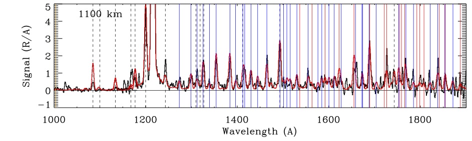
Figure 1: Observed (black) and simulated (red) limb spectra on Titan’s dayside during the 2016, DOY-015 PRIME observations. The top panel presents the average spectrum at 1100 km (100 km wide bin) demonstrating the strong Ly-α emission and the emissions from atomic (dashed lines) and molecular transitions (thin blue lines for LBH and thin red lines for VK bands).
References
- Lavvas P., Yelle R.V., Heays A.N., Campbell L., Brunger M.J., Galand M., Vuitton V., 2015. N2 state population in Titan’s atmosphere. Icarus, 260, p.29-59.
- Lavvas P., Galand M., Yelle R.V., Hayes A.N., Lewis B.R., Lewis G.,R. Coates A.J., 2011. Energy deposotion and primary chemical products in Titan’s atmosphere. Icarus, 213, 233-251.
How to cite: Lavvas, P. and Koskinen, T.: Titan’s atmospheric structure from Cassini/UVIS airglow observations, Europlanet Science Congress 2022, Granada, Spain, 18–23 Sep 2022, EPSC2022-447, https://doi.org/10.5194/epsc2022-447, 2022.
Introduction
With 13 years of observations, the Visual And Infrared Mapping Spectrometer (VIMS) onboard the \textit{Cassini} spacecraft has observed the surface and atmosphere of Titan through two seasons: winter and spring. In VIMS-IR spectra the surface is only seen in seven atmospheric windows due to the strong methane absorption. To retrieve the surface albedo we use radiative transfer (RT) models to compensate for the signal due to the atmosphere. Thanks to the lander Huygens, we have information about the optical properties of the aerosols above the equator that can be used in RT models. However, using the same aerosols vertical profile at high latitude doesn't work. With the help of the results of and Global Circulation Models and the Composite InfraRed Spectrometer onboard Cassini, we changed the aerosol vertical profile and optical properties in our RT model to better fit VIMS data at high latitude. While this model is not well constrained due to a lack of data, we manage to adjust the optical properties so our RT model based on Coutelier et al., (2021) retrieve surface albedo mostly between 0 and 1 instead of values crossing these boundaries like we had previously. It allow us to study with a RT model the shores and polar seas of Titan. We applied this new model on the same area of Kraken Mare in three consecutive VIMS cubes of the same flyby (subsequently named C1, C2 and C3). It allow us to validate our model on terrains with different albedo, and to notice an interesting feature in Kraken Mare that could be interpreted as sediment transport into the sea.
Adaptation of the aerosols optical properties and vertical profile
We decided to keep a 2 layers-based aerosol model, separated into haze and mist. We first changed the haze opacity vertical profile, using an exponential law : 
with the altitude of transition between mist and haze Ztr=70 km, and the scale height Hh=40 km. τh1µm is the opacity calculated by Doose et al., 2016 at 1 µm. We then changed the spectral slope of the optical depth of the mist with a simple power law as a first approximation :

with Δτmnorm the normalized optical depth of the atmospheric layer of mean altitude z, τhλ0 the total optical depth at λ0 = 1 µm calculated by Doose et al 2016., λ the wavelength, and the parameter b = 2.2 +/- 0.2
The most influent parameter is the mist single scattering albedo ωm. we decided to change it depending on that of the haze ωh and a factor α = 0.4 +/- 0.1.

Application and results on Kraken Mare
We tuned and applyed this model on three successive VIMS cubes (full names in Fig. 1) subsequently called C1, C2 and C3. We retrieved the albedo on a zone crossing Kraken Mare, containing pixels from land, shore and methane sea. They are circled in red in Fig.1. The top part shows the VIMS cubes, and the bottom part their footprint on the geomorphologic map of Titan. That way we can have an expectation on the retrieved albedo: dark in the sea, and bright on land.
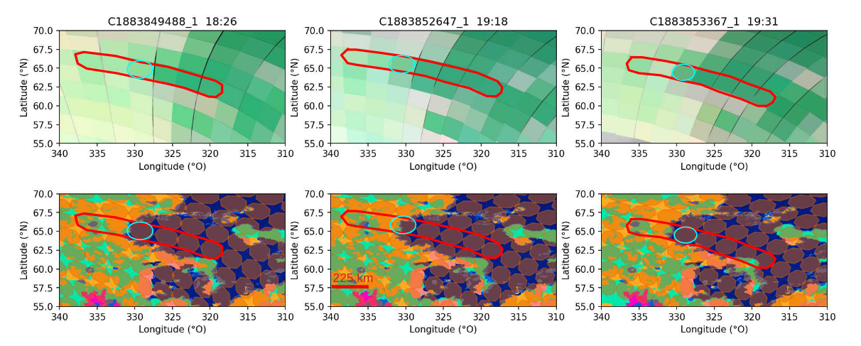
Figure 1 : (top) Successive VIMS cubes from flyby 292TI (colors : R : 5.01, V : 1.28, B : 2.79 μm).(bottom) : Footprint of the VIMS pixels on the geomorphologic map from Lopez et al., 2020. The pixels in our study are circled in red. The pixels circled in blue have mixed signatures.
The retrieved albedo are on Fig. 2. We still have remaining problems with negative albedo on dark pixels, mostly in the first atmospheric window. We can still differentiate very well the signatures from different terrains. Those coming from Kraken Mare are in blue, and those coming from the land are in green in Fig. 2. In C2, we have a pixel localized on the shore containing part of land and sea, circled in pink. Its signature is mixed, as we expected. However, we notice that on C1 and C3, two pixels localized in Kraken Mare (also circled in pink) also have a mixed signature. We did check that it was not a mistake in the cube geolocalization, or a difference due to a cloud.
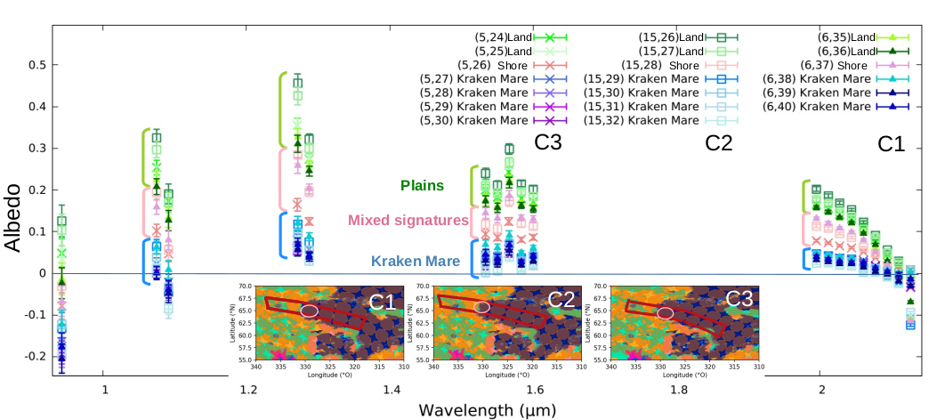
Figure 2 : Retrieved albedo of the selected pixels in Fig. 1. from the cubes C1, C2 and C3. The errors bar are calculated from the error on VIMS, and not from the error on the model. They are underestimated as a consequence.
Discussion
Infrared can penetrate deeply into liquid methane and ethane. The mixed signature we noticed can come from sediment transport carried by rivers flowing into Kraken Mare, issued from the erosion of the bedrock.
While this aerosol model for the poles is not exact, nor well constrained, the RT model is working and gives reasonable results on different cubes from the same flyby. We can compare the different surface albedos instead of the absolute values, because the atmospheric model is the same for all of the studied pixels. The combination of the RT analysis with the geomorphologic map is a powerful tool that leads to notice unexpected signatures.
With the seasons changes, we can expect that the improved polar aerosol model is not constant, so further studies should be made on other cubes through different seasons. We could that way follow through an other method the seasonal variation of the polar haze and mist layers.
References
Doose et al. (2016) Vertical structure and optical properties of Titan’s aerosols from radiance measurements made inside and outside the atmosphere. Icarus 270 : 355-375.
Coutelier et al. (2021) Distribution and intensity of water ice signature in South Xanadu and Tui Regio. Icarus 364 : 114464.
Lopes et al. (2020) A global geomorphologic map of Saturn’s moon Titan." Nature astronomy 4.3 : 228-233.
How to cite: Coutelier, M., Rannou, P., Cordier, D., and Seignovert, B.: Detection of sediment transport in Kraken Mare with a radiative transfert model using an aerosol vertical profile and optical properties adapted to Titan North pole, Europlanet Science Congress 2022, Granada, Spain, 18–23 Sep 2022, EPSC2022-449, https://doi.org/10.5194/epsc2022-449, 2022.
1. Introduction
Titan is the only moon in our solar system with a substantial atmosphere. It comprises 98% Nitrogen (Niemann et al., 2005), and is rich in hydrocarbon (CxHy) and nitrile (CxHyNz) species. Such species photochemically react to produce organic aerosols which compose a thick orange haze suspended in Titan’s middle atmosphere.
Global Circulation Models (GCMs) predict the meridional circulation in Titan’s stratosphere and mesosphere is dominated by a single pole-to-pole circulation cell for most of the Titan year (Hourdin et al., 1995; Newman et al., 2011; Lebonnois et al., 2012), and observations are broadly consistent with this prediction (Teanby et al., 2012, Vinatier et al., 2015). These models suggest circulation across the stratospheric equator, but this is not entirely consistent with what is observed. Existing studies show a North-South asymmetry in stratospheric haze abundance (Lorenz et al., 1997; de Kok et al., 2010), suggesting a mixing barrier near the equator. Here, we present a radiance ratio method for approximating latitudinal distributions of stratospheric HCN. We apply this to the region +/-30 degN and use HCN as a tracer to investigate the evolution and behaviour of the equatorial mixing barrier over the Cassini mission.
2. Observations
The Cassini spacecraft explored Saturn and its moons from 2004 to 2017. Throughout its 13-year exploration, Cassini performed 127 close flybys of Titan, observing at infrared, visible and ultra-violet wavelengths. One of Cassini’s twelve instruments, the Composite Infrared Spectrometer (CIRS) (Flasar et al., 2004; Jennings et al., 2017; Nixon et al., 2019) collected almost 10 million Titan spectra in the mid and far-infrared ranges (10 – 1500 cm-1), at a varied spectral resolution between 0.5 – 15.5 cm-1. In this study, we analyse low spectral resolution (~15 cm-1) observations collected by two CIRS focal planes, sensitive to wavenumber ranges 600 – 1100 cm-1 (FP3) and 1100 – 1500 cm-1 (FP4). Generally, low spectral resolution observations require shorter scan times so can be performed at a closer approach distance to Titan, hence achieving higher spatial resolution. This allows small spatial variations in atmospheric constituents to be resolved. Low-resolution observations also have good coverage of Titan’s equatorial region throughout the entire Cassini mission (Figure 1).
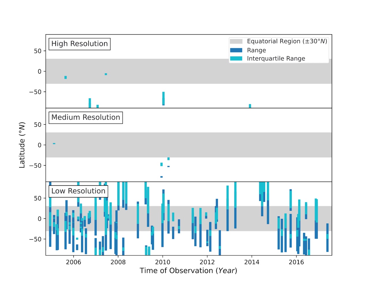
Figure 1: Mission coverage for the Cassini CIRS low spectral resolution nadir mapping observations.
3. Optimising Line-by-Line Retrieval Efficiency
Line-by-line (LBL) inversions in spectral analysis are computationally expensive. The correlated-k approximation (Lacis and Oinas, 1991) is often used to decrease the computation time of retrievals, but we found that it is not sufficiently accurate for these low spectral resolution and high signal-to-noise ratio observations (Figure 2c, d). In LBL modelling, a key parameter is the underlying spectral grid spacing. Finer grid spacing improves the forward model accuracy, but at a greater computation cost. To improve the efficiency of LBL runs, we determine a maximum grid spacing (Figure 2a, b) for which a LBL inversion will produce a sufficiently accurate spectrum in the shortest computation time. Typically, a single forward model run takes 2 hours for LBL, compared to 2 seconds for k-tables.
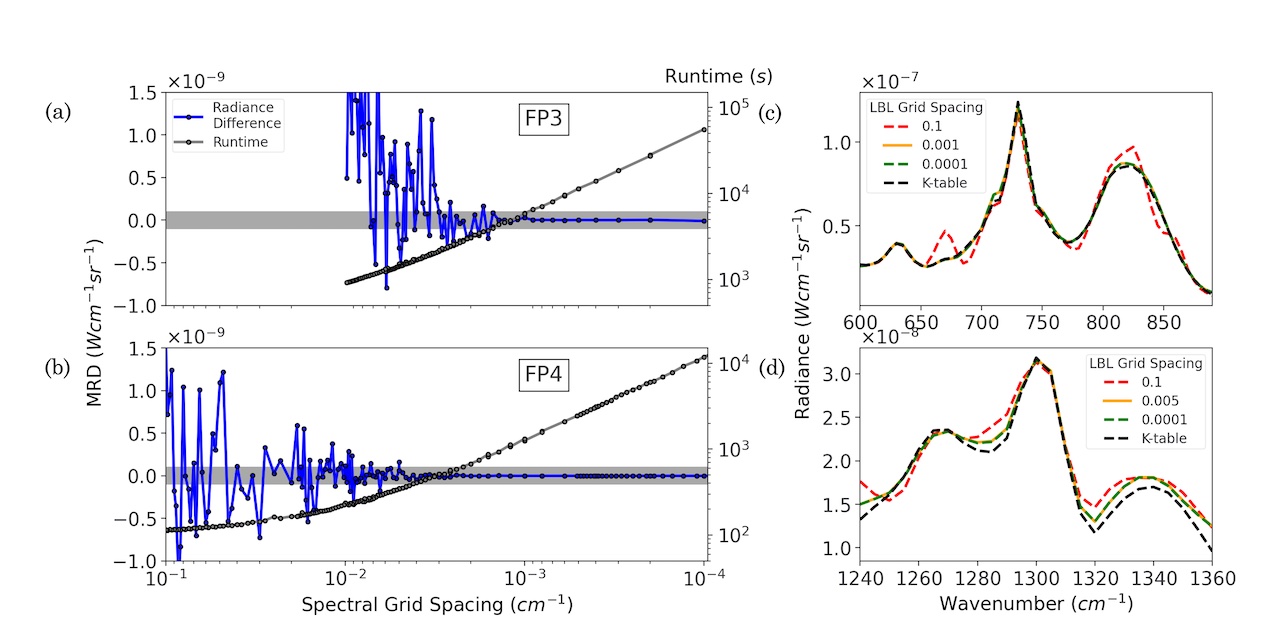
Figure 2: Comparison of spectra produced using a correlated-k (k-table) method and a line-by-line (LBL) method at varied spectral grid spacing. Maximum radiance difference (MRD) (a, b, blue line) between spectra produced at varied (0.1 – 0.0001 cm-1) and fine (0.0001 cm-1) grid spacing is assessed against a level of sufficient accuracy (a, b, grey area). The grid spacing determined to be optimal (0.001 cm-1 for FP3, 0.005 cm-1 for FP4) produces an almost identical spectrum to very fine (0.0001 cm-1) grid spacing (c, d) but at a significantly reduced runtime (a, b). A spectrum produced using a coarse grid spacing (0.1 cm-1) is shown for comparison. The spectrum retrieved using k-tables is not sufficiently accurate for these low-resolution observations (c, d).
4. Estimating Stratospheric HCN with a Radiance Ratio
We construct a radiance ratio formula for approximating HCN abundance from CIRS spectra, such that a greater number of observations can be analysed rapidly. Radiance ratios can be a useful tool for approximating gas contributions to a spectrum. They do not have the reliability of full spectral retrievals but require significantly less computation time. We compare the radiance ratio latitude dependence to full LBL retrievals of HCN, for a subset of our observations, to assess the reliability of our ratio method. LBL retrievals are performed using the Nemesis radiative transfer and retrieval code (Irwin et al., 2008) with our pre-determined optimal grid spacing. We calculate the radiance ratio for a set of approximately 20 low spectral resolution mapping observations (3 are shown in Figure 3).
There appears to be a sharp change in HCN abundance near the equator (Figure 3). This hints at a potential mixing barrier in Titan’s stratosphere. Furthermore, the position of this potential barrier appears to migrate over time. We use the results of this study to investigate dynamic processes in the equatorial region of Titan’s stratosphere and its evolution over the entire Cassini mission.
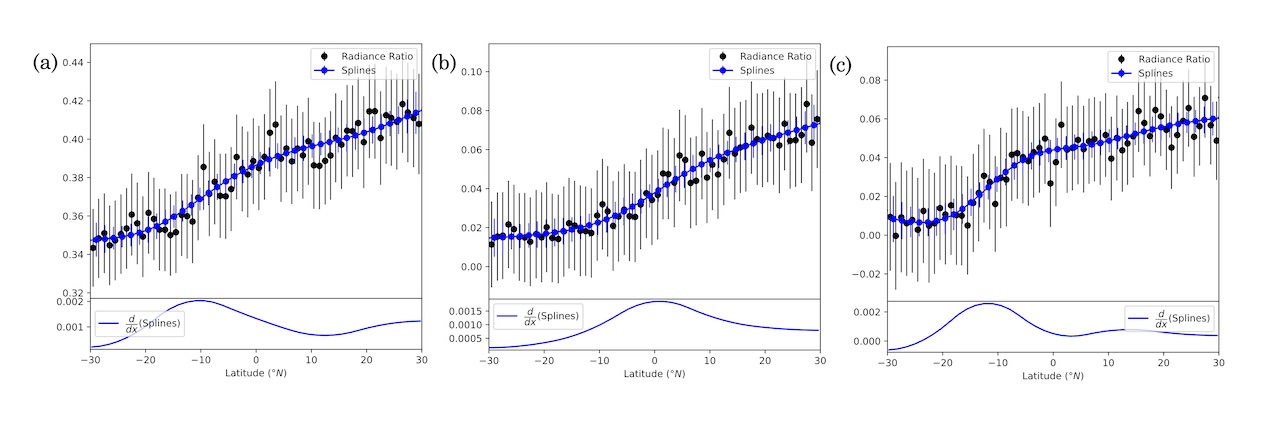
Figure 3: Our radiance ratio calculated for observations acquired on 08/2005 (a), 05/2006 (b) and 07/2012 (c). The radiance ratio is smoothed by fitting splines (Teanby, 2007). The gradient of each smoothed fit is also shown (bottom).
Acknowledgements
This research was funded by the UK Sciences and Technology Facilities Council.
References
de Kok, R., et al. (2010). https://doi.org/10.1016/j.icarus.2009.10.021
Flasar, F. M., et al. (2004). https://doi.org/10.1007/s11214-004-1454-9
Hourdin, F., et al. (1995). https://doi.org/10.1006/icar.1995.1162
Irwin, P., et al. (2008). https://doi.org/10.1016/j.jqsrt.2007.11.006
Jennings, D. E., et al. (2017). https://doi.org/10.1364/AO.56.005274
Lacis, A. A., & Oinas, V. (1991). https://doi.org/10.1029/90JD01945
Lebonnois, S., et al. (2012). https://doi.org/10.1016/j.icarus.2011.11.032
Lorenz, R. D., et al. (1997). https://doi.org/10.1006/icar.1997.5687
Newman, C. E., et al. (2011). https://doi.org/10.1016/j.icarus.2011.03.025
Nixon, C. A., et al. (2019). https://doi.org/10.3847/1538-4365/ab3799
Niemann, H. B., et al. (2005). https://doi.org/10.1038/nature04122
Teanby, N. A. (2007). https://doi.org/10.1007/s11004-007-9104-x
Teanby, N. A., et al. (2012). https://doi.org/10.1038/nature1161
Vinatier, S., et al. (2015). https://doi.org/10.1016/j.icarus.2014.11.019
How to cite: Wright, L., Teanby, N. A., Irwin, P. G. J., Nixon, C. A., and Mitchell, D. M.: Stratospheric HCN and Evolution of a Mixing Barrier in Titan’s Equatorial Region from Low-Resolution Cassini/CIRS Spectra, Europlanet Science Congress 2022, Granada, Spain, 18–23 Sep 2022, EPSC2022-463, https://doi.org/10.5194/epsc2022-463, 2022.
Introduction
With 13 years of observations, the Ion and Neutral Mass Spectrometer (INMS) onboard the Cassini spacecraft has observed the upper atmosphere of Titan through two seasons: winter and spring. The complex atmosphere is mainly composed of N2, CH4, H2 and Ar, but a lot more carbon and nitrogen bearing trace species have been observed by INMS and other instruments. Using data from the closed source neutral mode of INMS instrument, we studied the abundance and variation of traces neutral species in Titan ionosphere, between 1500 and 950 km of altitude. We will present an ongoing effort on the reanalysis of the entire INMS Titan's observation dataset.
Method
To do so we recalibrated INMS data by taking into account the dead time correction, the ram pressure enhancement, the saturation correction, the increase of pressure in the chamber with the decreases of altitude, the sensitivity and the contamination by thruster firing (Cui et al., 2009,2012). In addition, species entering the instrument were ionized and fragmented into ions inside INMS chamber, making difficult the identification of different species in such complex mass spectra. To retrieve the molecular mixing ratios we used a Monte-Carlo sampling on the fragmentation pattern to deconvolve the signal. To obtain a complete mass spectrum (m/z 1 to 99), we stacked INMS data, which increases the incertitude on the altitude. We used the mass spectra deconvolution code developed by Gautier et al., (2020), also employed by Serigano et al., (2020) when they treated Saturn INMS data.
This enabled the retrieval of vertical and seasonal variation of Titan's atmosphere minor components. We expect to be able to link our results with the seasonal variations observed by other instruments [such as CIRS (Mathé et al., 2020)] in lower atmospheric layers.
References
Cui et al.(2009) Analysis of Titan’s neutral upper atmosphere from Cassini Ion Neutral Mass Spectrometer measurements. Icarus 200 (2009) 581–615
Cui et al.(2012) The CH4 structure in Titan’s upper atmosphere revisited. J. Geophys. Res., 117, E11006, doi:10.1029/2012JE004222.
Gautier et al. (2020) Decomposition of electron ionization mass spectra for space application using a Monte-Carlo approach. Rapid. Com. Mass Spec. 34(8), e8659
Mathé et al., (2020) Seasonal changes in the middle atmosphere of Titan from Cassini/CIRS observations: Temperature and trace species abundance profiles from 2004 to 2017. Icarus, 344, 113547.
Serigano et al. (2020) Compositional measurements of saturn's upper atmosphere and rings from cassini INMS. Journal of Geophysical Research: Planets, 125(8), e2020JE006427.
How to cite: Coutelier, M., Gautier, T., Das, K., Serigano, J., and Horst, S.: Seasonal variation of trace species in Titan’s ionosphere, Europlanet Science Congress 2022, Granada, Spain, 18–23 Sep 2022, EPSC2022-479, https://doi.org/10.5194/epsc2022-479, 2022.
Introduction
Titan is the only moon in the solar system with a thick atmosphere, dominated by nitrogen and organic compounds and methane- and ethane-based climatic cycles similar to the hydrological cycle on Earth. Hence, Titan is a prime target for planetary and astrobiological researches. Heaviest organic materials resulting from atmospheric chemistry (including high atomic number aerosols) precipitate onto the surface and are subject to geological processes (e.g., eolian and fluvial erosion) that lead to the formation of a variety of landscapes, including dune fields, river networks, mountains, labyrinth terrains, canyons, lakes and seas analogous to their terrestrial counterparts but in an exotic context. Its optically thick atmosphere, however, prevents the surface from being probed in the entirety of the near-infrared (NIR) range, and its composition is still largely unknown, or largely debated at the least, preventing to fully understand and quantify the geological processes at play. Incident and reflected solar radiations are indeed strongly affected by gaseous absorption and aerosol scattering in the NIR. Only where the methane absorption is the weakest, a few transmission windows allow the detection of radiation coming from the low atmosphere and the surface, making possible to retrieve the surface albedo. In the 0.88-5.11 μm range (VIMS-IR channel), the Visual and Infrared Mapping Spectrometer (VIMS) instrument on board the Cassini spacecraft has shown that the surface can be observed in eight narrow transmission windows centered at 0.93, 1.08, 1.27, 1.59, 2.03, 2.69, and 2.78 μm, and in the 5.0-5.11 μm interval. Even in these transmission windows, residual gaseous absorption and increasing scattering from aerosols with decreasing wavelength make the analysis of the surface signal and the retrieving of surface albedo complex and delicate.
In order to retrieve the surface albedo in the atmospheric windows in the most possible rigorous way, we have developed a radiative transfer (RT) model with up-to-date gaseous abundances profiles and absorption coefficients and improved photochemical aerosol optical properties. We validated our model using in situ observations of Huygens-DISR (Descent Imager / Spectral Radiometer) acquired during descent and once landed. We then applied our RT model to the Selk crater area (the Dragonfly mission landing area) in order to map the surface albedo and discuss the surface properties of the different geomorphological units of the region.
Radiative transfer
Our RT model is based on the SHDOM solver to solve the RT equations using the plan-parallel approximation. Vertical abundance profiles and absorption lines of CH4 and isotopes, CO, C2H2 and HCN are implemented using the most recent studies. Correlated-k coefficients are used to calculate gases absorption coefficients at VIMS-IR spectral sampling and resolution. Aerosols extinction profile and single scattering albedo are described using a fractal code developed by [1], allowing the aerosol fractal dimension to be varied. Aerosols phase function is modified using a multi-angular VIMS sequence (Sébastien Rodriguez, personal communication). Our model is validated using the in situ observations of Huygens-DISR acquired during the complete descent sequence and once landed.
Application
We applied our RT model to the Selk crater region by inverting aerosol opacity and surface albedo over 4 VIMS cubes (1578266417_1, 1575509158_1, 1578263500_1, 1578263152_1) acquired over the area. We built local maps of aerosol opacities and surface albedos of the Selk region by combining the 4 VIMS cubes on a geographically projected mosaic (see the mosaic of the 4 raw VIMS observations in Fig. 1). A few longitudinal profiles of the retrieved atmospheric properties are shown in Fig. 2. Slopes and seams between cubes of the aerosol opacities, originally due to varying observation geometries between flybys, have been entirely corrected, confirming the robustness of our RT model and making the retrieved surface albedo more reliable. Retrieved surface albedo have been then corrected for the photometry using in-situ observations ([3]). The resulting albedo maps of the regions are highly contrasted and homogeneous, most of the seams between cubes (due to residual surface photometry) being corrected (Fig. 3).
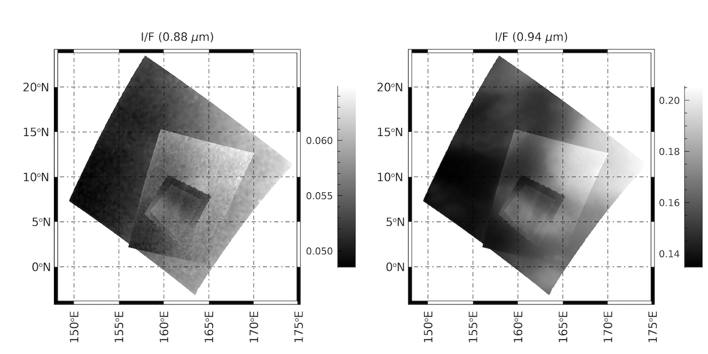
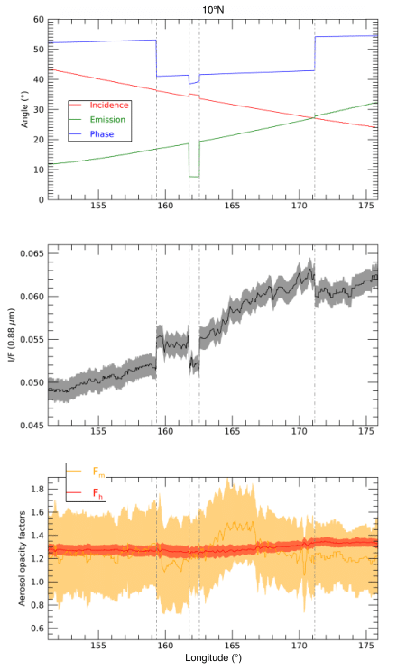
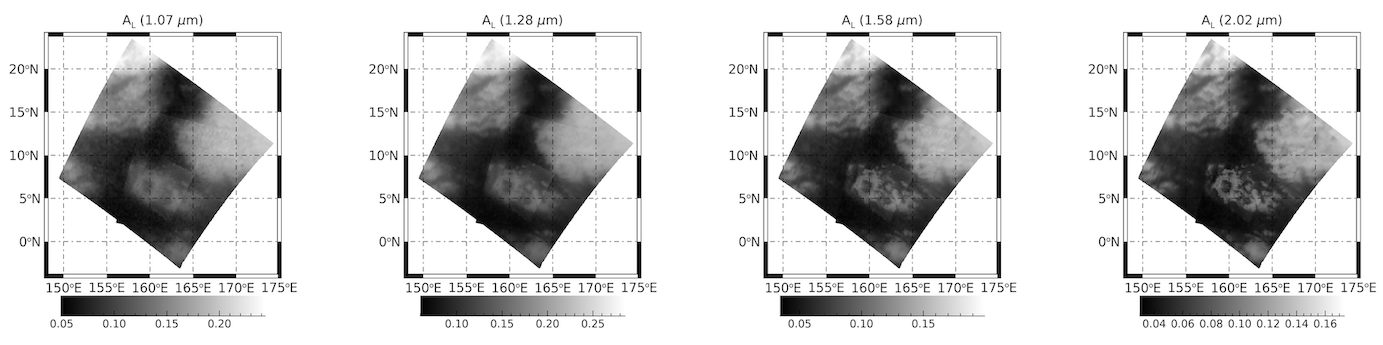
Conclusion
We developed and validated a new RT model for Cassini-VIMS observations of Titan with up-to-date atmospheric optical description. Coupled with an efficient inversion scheme, our model can be apply to the complete VIMS dataset for the retrieval of Titan’s atmospheric opacities and surface albedos at regional and global scales.
References
[1] Rannou, P., McKay, C., & Lorenz, R. 2003, Planetary and Space Science, 51, 963
[2] Karkoschka, E., Schröder, S. E., Tomasko, M. G., & Keller, H. U. 2012, Planetary and Space Science, 60, 342
How to cite: Es-Sayeh, M., Rodriguez, S., Coutelier, M., Rannou, P., Bézard, B., Maltagliati, L., Cornet, T., Grieger, B., Karkoschka, E., Seignovert, B., Le Mouélic, S., Sotin, C., and Coustenis, A.: Updated radiative transfer model for Titan in the near-infrared wavelength range: Validation on Huygens atmospheric and surface measurements and application to the analysis of the VIMS/Cassini observations of the Dragonfly landing area, Europlanet Science Congress 2022, Granada, Spain, 18–23 Sep 2022, EPSC2022-657, https://doi.org/10.5194/epsc2022-657, 2022.
In Titan, the two major gases - dinitrogen (N2) and methane (CH4) are ionized and/or photolyzed at high altitudes by the sunlight and the energetic particles from Saturn's magnetosphere, resulting in rich atmospheric chemistry and a wide variety of carbon and nitrogen-bearing atmospheric compounds. In the present work, we focus on studying the vertical profiles of trace species in the lower atmosphere to obtain a better insight into the atmospheric processes taking place on Titan.
To do so, we reanalyzed the data from the Gas Chromatograph Mass Spectrometer (GCMS) onboard the Huygens probe which executed its mission on 14th January 2005. The GCMS instrument sampled for nearly three and a half hours from an altitude of 146 km. It recorded data for two and a half hours in the atmosphere of Titan, then landed on the surface and kept on recording for another hour, after which the signal was lost. We analyzed the measurements made by direct sampling of the atmosphere (Niemann et al. 2010). These mass spectra obtained at different altitudes and pressure levels have been recalibrated to account for deadtime and saturation corrections to the measurements, set boundary conditions for the species, and considered sensitivity measurements from Cassini-Ion and Neutral Mass Spectrometer calibrations. We then analyzed the corrected mass spectra using Monte-Carlo deconvolution simulations. The simulations allow us to vary the peak intensities of fragmentation patterns of known species, which usually bears uncertainties on this kind of data, and then use a least-square fitting to deconvolve the mixed signals (Gautier et al. 2020, Serigano et al. 2020, 2022).
We present our ongoing effort to retrieve minor compounds' mixing ratios using this approach. As an example, the vertical profile of one of the trace species ethane (C2H6), is shown in figure 1.

Figure 1: Preliminary vertical profile of ethane (C2H6) mixing ratio
In the future, we plan to extend this study to develop a sub-surface model of Titan which will help us understand the outgassing of methane that was observed by the probe upon its touchdown on the surface.
References:
Niemann et al. Composition of Titan’s lower atmosphere and simple surface volatiles as measured by the Cassini-Huygens probe gas chromatograph mass spectrometer experiment. JGR 115, E12006, 2010
Gautier et al. Decomposition of electron ionization mass spectra for space application using a Monte-Carlo approach. Rapid. Com. Mass Spec. 34(8), e8659 (2020)
Serigano et al. Compositional measurements of Saturn’s upper atmosphere and rings from Cassini INMS. JGR:Planets, 125 (8), E006427 (2020)
Serigano et al. Compositional Measurements of Saturn’s Upper Atmosphere and Rings from Cassini INMS: An extended Analysis of Measurements from Cassini’s Grand Finale Orbits. JGR:Planets, 127, E007238 (2022)
How to cite: Das, K., Gautier, T., Serigano, J., Szopa, C., Hörst, S. M., Coutelier, M., Vinatier, S., and Trainer, M. G.: Study of volatile compounds in the atmosphere of Titan, Europlanet Science Congress 2022, Granada, Spain, 18–23 Sep 2022, EPSC2022-710, https://doi.org/10.5194/epsc2022-710, 2022.
The Cassini cameras and especially the Visual and infrared Mapping Spectrometer has provided a sequence of spectra showing the diversity of Titan’s surface spectrum from flybys performed during the 13 years of Cassini’s operation. The investigation of Titan’s surface chemical composition is of great importance for the understanding of the atmosphere-surface-interior system of the moon. The Soi crater region with the well-preserved Soi crater in its center, spans from Titan’s equatorial regions to high northern latitudes. This provides a rich diversity of landscapes, one that is also representative of the diversity encountered across Titan. We mapped this region at 1:800,000 scale using Cassini SAR and non-SAR data and produced a geomorphological map using the methodology presented by [1] and [2]. The VIMS coverage of the region allowed for detailed analysis of spectra of 262 different locations using a radiative transfer technique [3;4] and a mixing model [5;6], yielding compositional constraints on Titan’s optical surface layer. Additional constraints on composition on the near-surface substrate were obtained from microwave emissivity. We identified 22 geomorphological units, 3 of which were not previously described, and derived combinations of top surface materials between dark materials, tholin-like materials, water-ice, and methane. We found no evidence of CO2 and NH3 ice. We also observe empty lakes as far south as 40°N, which mark the most southern extent of Titan’s north polar lakes. We use the stratigraphic relations between our mapping units and the relation between the geomorphology and the composition of the surface layers to build hypotheses on the origin and evolution of the regional geology.
[1] Malaska, M., et al. (2016), Icarus 270, 130; [2] Schoenfeld, A., et al. (2021), Icarus 366, 114516; [3] Solomonidou, A., et al. (2014), J. Geophys. Res. Planets, 119, 1729; [4] Solomonidou, A., et al. (2016), Icarus, 270, 85; [5] Solomonidou, A., et al. (2018), J. Geophys. Res. Planets, 123, 489; [6] Solomonidou, A., et al. (2020), A&A 641, A16.
How to cite: Solomonidou, A., Schoenfeld, A., Malaska, M., lopes, R., Coustenis, A., Birch, S., Le Gall, A., and Schmitt, B.: Chemical composition analysis of Titan’s equatorial and midlatitude surface regions, Europlanet Science Congress 2022, Granada, Spain, 18–23 Sep 2022, EPSC2022-776, https://doi.org/10.5194/epsc2022-776, 2022.
OPS3 | Icy ocean worlds: Past and future explorations
The NASA program exploring habitability places in the outer Solar System searches for simple forms of life in icy moons of Giant Planets, with internal oceans off thermal equilibrium between cold, iced surface and rocky center warmed, possibly by dissipation of tides from the Planet; H2O molecules might lose oxygen to reduced bottom minerals, and get oxygen back when moving upwards. This Ocean World concept was confirmed in Jupiter’s moon Europa, and Saturn’s moons Titan and Enceladus, the last one ejecting a local plume through ice, though not Titan, with the Europa-plume case apparently confirmed. In 2017, H2 molecules, considered sign of life, were detected at the Enceladus plume. We here propose a mission to explore the only large Neptune moon, Triton, which is usually considered an important Kuiper Belt Object as captured dwarf planet. More relevant, here, is that Voyager 2, in 1989, found evidence of Triton ejecting a kind of plume.
Ice Giants, however, have only received flyby missions, at difference with Gas Giants: An effective orbiter-type mission to faraway Neptune is acknowledged as extremely expensive, trip-average solar power is almost nil, chemical capture leads to high wet-mass, with scientific load and orbital maneuvers very constrained. NASA had set a nuclear reactor in space for on-board S/C power in April 1965 but afterwards, for safety considerations, it always used a Radioisotope Pu 238 power system (helpful in mission Cassini). In a sense constraints trade occurred in 2009, between proposed Triton missions a) with full modern technology but just a flyby (EPSC/Potsdam) and b) captured orbiter though with minimum technology (National Research Council / Planetary Science Decadal Survey). Aerocapture and Radioisotope, for propulsion and power, have been considered for Neptune missions, but decayed consideration.
Magnetic Solution to Power and Propulsion Issues
Icy moon missions could use, however, thin, multi-kilometer conductive tethers, with no power or propulsion needs, available to a S/C if passing near the planet. The planetary magnetic dipole allows free –thermodynamically dissipative- S/C capture, and afterwards maneuvering: The relative S/C velocity induces a motional electric field Em (in the tether frame) in the highly conductive plasma around, which polarizes the tether and drives a current I inside, with I ·Em > 0, the field B then exerting Lorentz drag on the current. Driving, however, was ineffective in tethers standard in the 90`s such as TSS1 and TSS1R, insulated all along, with a conductive sphere large enough at the anodic end, typically implying radius much greater than ambient Debye length and thermal electron gyroradius, strongly reducing electron collection. Bare tethers [1] eliminated sphere and insulation to allow electron collection over a resulting anodic tether segment, as a giant cylindrical Langmuir probe, in the optimal OML (orbital-motion-limited) regime. Laframboise and Parker [2] had proved that OML current to cylindrical probes of convex cross-section and equal perimeter p are equal. Thin tape cross-section will reduce tether mass when compared to an equal p tether with round cross-section. Bare tethers, which made standard tethers rapidly obsolete, will thus be characterized by all 3 dimensions, length, width and thickness, widely differing, allowing particular design easier.
Lorentz drag decreasing as the inverse 6th power of radial distance to dipole, capture periapsis would need be very close to the Planet. Keeping current on following capture would hardly affect it, whereas apoapsis could be lowered to finally reach 1:1 Laplace resonance of S/C and moon of interest.
Bare Tether Validation and Use
Bare-tether analysis was validated in early 2001 in an unintended way [3]. Measurements at the International Space Station involving 3 NASA Centers, NOAA/Boulder. Univ-Houston and SAIC, showed on-board plasma-contactors ejecting substantial electron current as if ISS structure had become very negative. Authors acknowledged in the Abstract that tensioning rods of solar array masts could collect ambient electrons as bare-wire tethers, with modeling “based upon J.R. Sanmartin’s bare-wire collection theory’, which was incorporated into the complex ISS computer code, Environment Work Bench, including models of Station, orbital motion, earth’s magnetic field, and ionosphere.
Further, in 2007, Vlasov-code simulations in the high–bias OML regime, at an Unuversity of Michigan PhD Thesis by E. Choinière on the electron density versus radial distance [4] were shown equal to a high approximation when compared [5] with detailed results from the bare-tether theory.
To date, the bare tether analysis has been applied in considering missions to moons Europa [6] and Enceladus [7], and to Ice Planet Neptune [8]}
References
[1] JR Sanmartin, M Martinez-Sanchez, E Ahedo, J. Prop & Power 9, 353-360, 1993
[2] JG Laframboise, LW Parker, Phys. Fluids 16 629-636, 1973
[3] EA Bering et al, Paper 2002-0935, 40th AIAA Aerospace Sciences Meeting and Exhibit, Reno, NV, 14-17 Jan 2002
[4] E Choinière, BE Gilchrist, IEE Trans on Plasma Science 35, 7-22, 2007
[5] JR Sanmartin, E Choinière, BE Gilchrist, J-B Ferry, M Martinez-Sanchez, IEE Trans in Plasma Science 36, 2851-2858, 2008
[6] JR Sanmartin et al, J. Prop & Power 33, 338-342, 2017
[7] JR Sanmartin, J Pelaez, Acta Astronautica 168, 200-203, 2020
[8] JR Sanmartin, J Pelaez, Acta Astronautica 177, 906-911, 2020
How to cite: Sanmartin, J. and Pelaez, J.: Exploring moon Triton, Europlanet Science Congress 2022, Granada, Spain, 18–23 Sep 2022, EPSC2022-39, https://doi.org/10.5194/epsc2022-39, 2022.
To assess the potential habitability of Europa, it is important to understand its chemical composition (Hand et al., 2007). Young terrain features on Europa’s surface likely consist of material up-welled from the liquid water source below (Wilson et al., 1997; Pappalardo et al., 1998; McCord et al., 1999; Figueredo and Greeley, 2004; Mével and Mercier, 2007), encoding relevant compositional information. A major science objective of NASA’s Europa Clipper mission is to characterize the composition of young terrain features using data acquired on close flybys. The Surface Dust Analyzer (SUDA) is an in situ instrument that collects and analyzes the composition of individual grains (Kempf et al., 2012), which are ejected from Europa’s surface by a continuous bombardment of interplanetary impactors (Krüger et al., 1999, 2003; Goode et al., 2021). By applying a dynamical model to these particles, we compute the probability of SUDA’s detections originating from a given feature along the flyby trajectory based on Monte Carlo (MC) simulations. The time-of-flight (TOF) mass spectra that characterizes the chemical composition of individual grains results in a time series of various compositional types along the flyby. We present here a method to analyze a time series of compositional spectra recorded by SUDA that provides a robust estimate for the abundance of different compositional types on the surface, resolved for features along the ground track of the flyby. By demonstrating the association of compositional detections with geological sites of origin, data collected by SUDA is used to infer the compositional ground truth for young terrain features on Europa.
How to cite: Goode, W., Kempf, S., and Schmidt, J.: Mapping the composition of Europa’s young terrain features with SUDA, Europlanet Science Congress 2022, Granada, Spain, 18–23 Sep 2022, EPSC2022-150, https://doi.org/10.5194/epsc2022-150, 2022.
1. Introduction
Liquid water reservoirs in Europa's icy crust, if they exist, could represent the most accessible liquid water bodies in the outer solar system. Previous studies have demonstrated that freezing cryoreservoirs might trigger eruptions due to the pressurization associated with volume change as liquid water expands to become water ice [1, 2]. Locating potentially stored and erupted brines is key for the exploration of ocean worlds and the search for habitability and life beyond Earth.
Here, we aim to numerically model the coupled chemical evolution and pressurization of freezing brines stored in Europa’s ice shell using current best estimates of the oceanic composition [3] to predict the composition of erupted cryolava. This composition varies with time, as salts concentrate during freezing [4], which could lead to erupted brines of varying composition depending on the reservoir frozen fraction when the eruption is triggered. This could explain the variations of albedo observed around features potentially associated with cryovolcanism, for example smooth plains, as shown in Fig. 1.
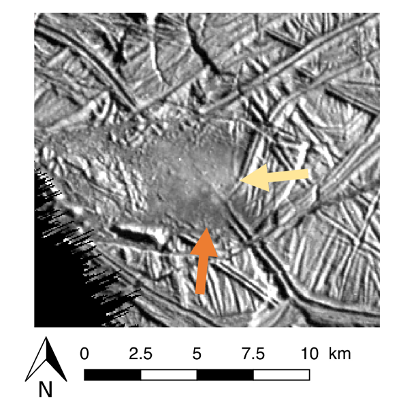
Figure 1: Smooth plain on Europa’s surface with morphology consistent with eruption of liquid cryolava [1]. The yellow and orange arrow indicate two areas of different albedo, which may have been emplaced by two eruptive events of brines of different composition. NASA Galileo image 9352r.
2. Methods
Cryomagma chemistry Whether they are formed by in-situ melting [5] or intrusion of oceanic water [6], the best estimate for cryomagmatic fluid composition is provided by models of evolution of Europa’s interior and ocean. An example cryomagma composition used in our model, consistent with oceanic compositions predicted by recent literature [3], in wt.%, is 99.0% H2O, 0.32% Na, 0.28% Cl, 0.16% bicarbonate, 0.21% sulfate, 0.027% K, 0.013% Ca, and 0.002% Mg. The equilibrium freezing of oceanic brines is modeled using the software PHREEQC [7] to obtain the liquid and solid fraction of each component of the aqueous solution as a function of the temperature. We use these data as an input of the model presented below.
Model principle Previous studies [1, 2] demonstrated that internal overpressure increases in potential freezing cryoreservoirs as cryomagma transitions to the less-dense solid phase. The critical freezing time required to break the reservoir and trigger an eruption is a function of the reservoir chemical and physical parameters (see example in Fig. 2 for a spherical 500 m radius reservoir located 2 km below the surface and filled with pure liquid water [1, 2]). The cryomagma chemical evolution during freezing will affect the solution and formed ice densities, and can thus make the critical freezing time different from what was calculated by previous studies. We thus need to model the cryomagma composition and internal overpressure as coupled variables. By doing so, we will be able to predict a realistic critical freezing time to trigger eruptions, as well as the
cryomagma composition when the eruption begins.
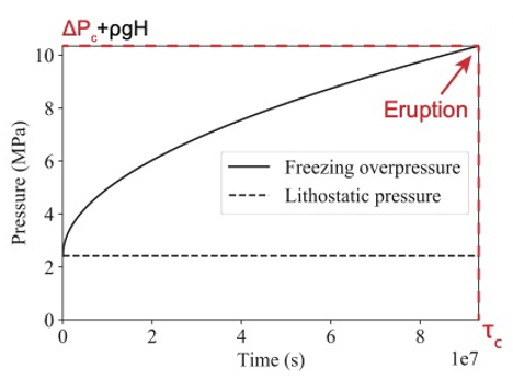
Figure 2: Pressure as a function of the time in a 500 m radius freezing cryoreservoir located 2 km below the surface. Here the cryomagma is composed of pure water only [2].
Numerical procedure We couple temperature-dependent compositional outputs from PHREEQC with a 1D numerical simulation using the finite differences method to simulate a freezing cryoreservoir. At each time step (i.e., reservoir temperature), we vary the composition of the formed ice and remaining aqueous solution. We modify several parameters accordingly, such as the liquid and solid densities and thermal conductivities. We ensure the energy and mass are conserved through time by calculating the cryomagma frozen fraction that balances the heat lost during each time step. As an output of the model, we can obtain the temporal evolution of: (i) the temperature in the reservoir, (ii) the composition of the formed solid and the remaining liquid and (iii) the internal overpressure. Finally, we can predict the composition of the erupted brines once (and if) the eruption is triggered.
Cyclic eruptions After the first eruption, cryomagma reservoirs may keep freezing and trigger several other eruptions as evoked in Lesage et al. [8]. We added the possibility to continue freezing and trigger several eruptions to our numerical simulation so that we can observe the evolution of erupted brines composition through time.
3. Preliminary results
Initial results demonstrate that salts concentrate in the reservoir during freezing, which decreases the solution freezing temperature and can make the freezing slower than expected with simpler models [1, 2]. On the other hand, the ice formed is initially mostly composed of pure liquid water and thus has a low density compared to the remaining liquid, which can accelerate the pressurization. The effect of both these mechanisms on the critical freezing time have to be quantified. The concentration of non-water components through time is also expected to result in cryolava flows with darker albedo and varying spectral signatures in the case of repeated eruptive events. These results will inform the upcoming missions JUICE (ESA) [9] and Europa Clipper (NASA) [10] on the spectral signatures that could indicate the presence of shallow sub-surface cryoreservoirs and provide information on their activity.
Acknowledgements
Portions of this research were carried out at the Jet Propulsion Laboratory, California Institute of Technology, under contract with the National Aeronautics and Space Administration (NASA). This work was supported by Scientific Exploration Subsurface Access Mechanism for Europa (SESAME) grant number 80NSSC19K0614 and by NASA’s Solar System Workings program (#80NSSC20K0139). The PHREEQC routine is available at https://github.com/MarcNeveu/frezchem.
References
[1] Lesage E. et al. (2020) Icarus, 335, 11336, [2] Lesage E. et al. (2022) The Planetary Science Journal, in press., [3] Melwani Daswani et al. (2021) Geophysical Research Letters, 48(18), [4] Zolotov M. Y. & Kargel J. S. (2009) Tucson, AZ: University of Arizona Press, [5] Kalousová et al. (2016) Journal of Geophysical Research: Planets, 121(12), 2444-2462, [6] Craft K. L. et al. (2016) Icarus, 274, 297-313, [7] Parkhurst, D. L. (1995). User's guide to PHREEQC, [8] Lesage et al. (2021) Icarus, 361, 114373, [9] Grasset O. et al. (2013) Planetary and Space Science, 78, 1-21, [10] Howell S. M. and Pappalardo R. T. (2020) Nature Communications, 11, 1311.
How to cite: Lesage, E., Howell, S. M., Naseem, M., Neveu, M., Melwani Daswani, M., and Vance, S. D.: Chemical composition of erupted brines on Europa, Europlanet Science Congress 2022, Granada, Spain, 18–23 Sep 2022, EPSC2022-301, https://doi.org/10.5194/epsc2022-301, 2022.
Context: Enceladus, an icy moon of Saturn, possesses an internal water ocean and geysers expelling ocean material into space. Cassini investigations indicated the ocean could be habitable and has a complex interaction with the rocky core. Further investigation of the composition of the plume formed by the geysers is necessary to fully understand the ocean, its possible habitability, and what it tells us about Enceladus’ origin.
Mission profile: Moonraker has been proposed as an ESA M-class mission designed to orbit Saturn and perform multiple flybys of Enceladus, focusing on traversals of the plume. Moonraker consists of an ESA-built platform, with strong heritage from JUICE (and Mars Sample Return for solar power), and carrying a suite of instruments dedicated to plume and surface analysis. The nominal Moonraker mission includes a 23-flyby segment, with the possibility of expanding the mission with additional similar segments, depending on available resources.
Objectives and expected impact: Moonraker is devoted to the investigation of i) the habitability conditions of present- day Enceladus and its internal ocean, ii) the mechanisms at play for the communication between the internal ocean and the surface of the South Polar Terrain, and iii) the formation conditions of the moon in the context of the formation of the Saturnian system. Moonraker, thanks to state-of-the-art instruments that represent a vast improvement over Cassini’s payload, would quantify the abundance of key species in the plume, isotopic ratios, and physical parameters of the plume and the surface. Such a mission would allow to solve the standing questions left by Cassini on the aforementioned topics as well as pave the way for a possible future lander mission.
How to cite: Mousis, O., Bouquet, A., Langevin, Y., André, N., Durry, G., Hartogh, P., Helbert, J., Iess, L., Kempf, S., Masters, A., Postberg, F., Renard, J.-B., Vernazza, P., Vorburger, A., and Wurz, P. and the Moonraker team: Moonraker - an Enceladus Multiple Flyby Mission Submitted to the ESA 2021 M-class Call, Europlanet Science Congress 2022, Granada, Spain, 18–23 Sep 2022, EPSC2022-329, https://doi.org/10.5194/epsc2022-329, 2022.
Introduction
Europa's surface is the youngest of the icy satellites and shows signs of recent activity [1]. The main driver of this activity is Jupiter’s tidal forces which are responsible for the existence of a global water ocean underneath Europa’s icy crust [2]. This ocean is thought to be in a direct contact with the rocky mantle [3] creating a potential environment for the emergence of life.
This places Europa at the center of future space exploration with NASA’s Europa Clipper mission [4] as well as ESA’s JUpiter ICy moons Explorer (JUICE) that will more generally study the Jovian icy moons [5].
To prepare for those missions, it is crucial to get the most out of the data we currently have. Photometry plays a key role in deriving remote sensing science products. As such, photometric correction is often the first step of any remote sensing analysis such as mapping or spectroscopy. In itself, photometry is closely linked to the surface microtexture and can help us better understand its physical state [e.g. 6, 7].
In this work, we are deriving photometric parameters for selected areas of Europa - we analyze their spectral dependency and how that can be translated into physical properties.
Dataset
We are revisiting data from Galileo’s Near Infrared Mapping Spectrometer (NIMS) [8] that operated between 0.7 – 5.2 m.
Calibrated and georeferenced data cubes (g-cubes) archived in the PDS Imaging Node have been stored in a database [9] with relevant information such as longitude, latitude, wavelengths, reflectance value, photometric angles etc. This tool allows for a comprehensive view of the dataset and quick exploration to assess the surface and angle coverage available for our study.
Due to changes in the wavelengths calibration and detector failures during operations, the phase angle coverage is very variable across the spectrum (from one cube to the other) with ranges from a few degrees to 80 degrees. We favor spectral intervals with a dense phase coverage. Moreover, to accommodate the shift in the wavelengths reference over time as well as to maximize our geometric diversity, we will not be looking at specific wavelengths but at 40 nm wide ranges of wavelengths across the spectrum.
We retrieved the reflectance and geometry information for a selection of regions of interest across the surface (Figure 1) by finding a compromise between interesting regions and relevant phase angle and spectral coverage.
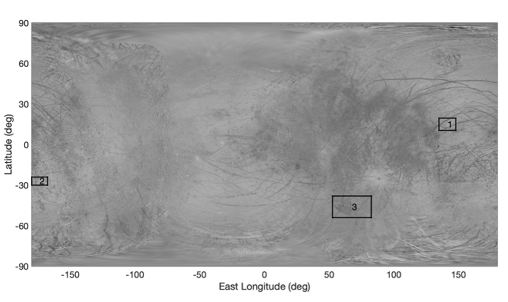
Figure 1: Map of Europa (credits: Björn Jónsson) with studied areas highlighted
Estimation of photometric parameters
For each area we are considering, we estimated a set of photometric parameters for every 40 nm wavelength interval we have defined. For this work, we are considering Hapke’s direct model detailed in [10] and [11]. Six parameters are to be estimated: phase function (b, c), single-scattering albedo (ω), rugosity (θ ̅), opposition effect (h and B_0).
We used an estimation method based on Bayesian statistics and that we developed for our regional studies of Jupiter’s icy moons in the visible [12, 13, 14]. This allows for of the parameters was inferred except for their physical domain of variation. The posterior Probability Density Functions (PDFs) are sampled with a Monte Carlo Markov Chain algorithm.
Results
We analyzed the different parameters over our three areas of study. Results were very heterogeneous in terms of accuracy across the spectrum but it is clear that the photometric parameters do vary somewhat with the wavelength, as also observed in laboratory experiment [15].
Figure 2 shows the example of the single-scattering albedo and macroscopic roughness estimations between 700 nm and 5 μm for ROI#1 in the leading hemisphere and a sample of wavelengths for which we have well constrained results.
Even though with naïve theoretical considerations we would expect a constant roughness - independent of wavelength - we found here that θ ̅ seems to become more important with higher wavelengths and lower reflectance. This could be related to specific absorption patterns or the presence of certain inclusions that would influence the photometric behavior in preferred wavelengths. In addition, roughness, as observed at various scales determined by the wavelength, may differ in natural material. This phenomenon is known as scale dependence roughness and may play a role here. Here we confirm the first-order dependence of absorptivity and roughness, determined in laboratory measurements [15].
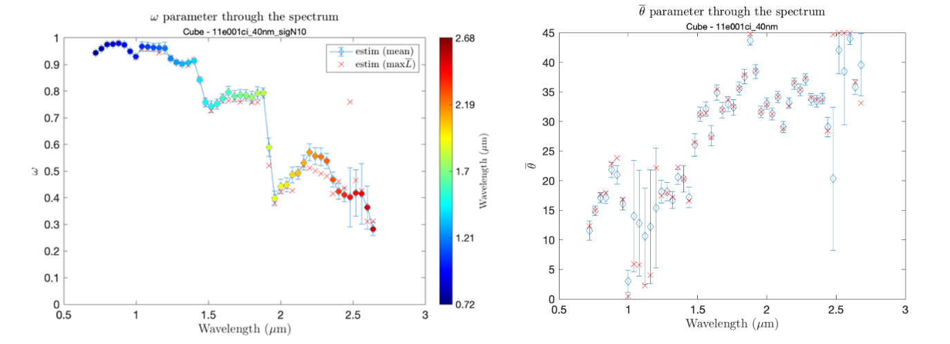
Figure 2: Spectral evolution of the single scattering albedo (left) and the macroscopic roughness (right) for ROI#1 estimated via mean of posterior distribution (blue) and maximum likelihood (orange)
Conclusion and future work
Based on this work, we aim at locally derive photometric corrections that can be used for other remote sensing products like mapping and spectroscopy. The physical implications of a spectrally dependent macroscopic roughness or phase function might also contribute to a better understanding of the history of Europa’s surface and will be our primary focus going forward.
Studying the spectral dependence of the Hapke parameters specifically is interesting as this model is one of the most widely used to investigate radiative transfer in relation to planetary surfaces. Nonetheless, a lot of different photometric models could also be considered. We plan to complement this work by studying the spectral dependency of other photometric models [e.g. 14, 16].
References
[1] Pappalardo, R. T. et al. (1999) JGR: Planets, 104 (E10) :24015_24055. [2] Carr, M. H. et al. (1998) Nature. [3] Vance, S. D. et al. (2018) JGR: Planets, 123. [4] Phillips, C. B. and Pappalardo, R. T. (2014) Eos, Transactions American Geophysical Union. [5] Grasset, O. et al. (2012) Planetary and Space Science. [6] A. McGuire, A. and Hapke, B. (1995) Icarus. [7] Souchon, A. et al. (2011) Icarus. [8] Carlson, R. W. et al (1992) Space Science Review. [9] Cornet, T. et al. EPSC 2022. [10] Hapke, B. (1993) Cambridge University Press. [11] Hapke, B. (2002) Icarus, vol. 157. [12] Schmidt, F. and Bourguignon, S. (2019) Icarus. [13] Belgacem, I. et al. (2019) Icarus. [14] Belgacem, I. et al. (2021) Icarus, vol 369. [15] Pilorget, C. et al., (2016) Icarus [16] Oren, M., Nayar, S. K. (1994) SIGGRAPH94.
How to cite: Belgacem, I., Cornet, T., Schmidt, F., Cruz Mermy, G., Andrieu, F., and Altobelli, N.: Spectral variation of Europa’s regional photometry, Europlanet Science Congress 2022, Granada, Spain, 18–23 Sep 2022, EPSC2022-359, https://doi.org/10.5194/epsc2022-359, 2022.
There is a volatiles enrichment in planetary bodies with the distance from the Sun because the lower temperatures caused their condensation during the solar system formation. As a consequence, the role of volatiles in the geochemistry and thermal evolution became important on certain bodies of the outer solar system, such as the ocean worlds. In order to understand both, physico-chemical interactions between volatiles and salts or other minerals also present in the internal aqueous reservoirs should be characterized. In this regard, the H2O-CO2-Na2CO3-NH3-CH3OH system is a potential candidate to be present within some ocean worlds, such as Enceladus, Titan and Triton. Whereas carbon dioxide (CO2) has been widely detected on icy satellites [e.g., 1-3], signatures of other volatiles such as ammonia (NH3) and methanol (CH3OH) are scarce and have only been found in low concentrations [4], despite their presence is theoretically expected [5-8]. A plausible explanation for the absence of these volatiles on icy moon surfaces is that they reacted at the interior with other substances, forming new compounds [9]. In addition, we included carbonates in our experiments since they are found in carbonaceous chondrites that have suffered low-temperature hydrothermal alteration, and therefore might be considered to come from the outer region of the solar system [10].
In this presentation we will show the results of the Raman spectroscopy kinetic study of the systems H2O-CO2-NH3, H2O-CO2-NH3-CH3OH, H2O-Na2CO3-NH3, and H2O-Na2CO3-NH3-CH3OH, which were exposed to temperatures down to 230 K and pressures up to 50 MPa. From the Raman spectra taken in situ throughout the experiments performed in a high-pressure cell, we were able to monitor the changes in pH of the systems by analyzing the carbonate-bicarbonate ion peak intensity ratio at each time step due to variations in aqueous chemical speciation and precipitation of solids. Our experiments also allowed us to evaluate the active role of CH3OH in the redox equilibria of the systems over time. Finally, the solubility of the carbonates formed was also investigated first, in a CO2 atmosphere, and then at high-pressure water.
This study is the progress of a previous work carried out by differential scanning calorimetry (DSC) [11], where we confirmed that CO2 clathrates stabilize in coexistence with carbonates. In this work, we observed that the presence of salts and volatiles during clathrate formation affect their level of cage occupancy, resulting in less-stable partially-filled structures with low dissociation enthalpies.
This work is funded by the Spanish State Research Agency (AEI) Project No. MDM-2017-0737 Unidad de Excelencia "María de Maeztu"- Centro de Astrobiología (CSIC-INTA). We also acknowledge support from the Spanish MINECO project PID2019-107472RB-C32.
References:
[1] Hansen and McCord. Geophys. Res. Lett. 2008, 35 (1), L01202.
[2] Cruikshank et al. Icarus 2010, 206 (2), 561–572.
[3] Grundy et al. Icarus 2006, 184 (2), 543–555.
[4] Grasset et al. Space Sci. Rev. 2017, 212 (1), 835–875.
[5] Sohl et al. Space Sci. Rev. 2010, 153 (1), 485–510.
[6] Deschamps et al. Astrophys. J. 2010, 724 (2), 887–894.
[7] Dougherty et al. J. Geophys. Res. Planets 2018, 123 (12), 3080–3087.
[8] Tobie et al. Icarus 2005, 175 (2), 496–502.
[9] Kargel. Icarus 1992, 100 (2), 556–574.
[10] Johnson and Prinz. Geochim. Cosmochim. Acta 1993, 57 (12), 2843–2852.
[11] Muñoz-Iglesias and Prieto-Ballesteros. ACS Earth Space Chem. 2021, 5 (10), 2626–2637.
How to cite: Munoz-Iglesias, V., de Dios-Cubillas, A., and Prieto-Ballesteros, O.: Physico-chemical evolution of the H2O-CO2-Na2CO3-NH3-CH3OH system at low temperatures and high pressures. Implications for icy ocean worlds., Europlanet Science Congress 2022, Granada, Spain, 18–23 Sep 2022, EPSC2022-393, https://doi.org/10.5194/epsc2022-393, 2022.
The JUpiter ICy moons Explorer (JUICE), the first large-class of the European Space Agency (ESA), is planned to launch in 2023, and one of its main goals is to make detailed observations of Jupiter’s moon Ganymede. The mission will investigate the past and/or recent cryovolcanic and tectonic activity of the moon and the exchange processes with the subsurface and possibly with the ocean. Recently, the science team defined “potential cryovolcanic regions” as a category of high interest for observation by JUICE (Stephan et al., 2021). For preparation of the scientific return of the mission, it is important to study in detail the regions that are considered to be good candidates for past/present activity. Light material areas on Ganymede imaged by Voyager have been suggested to represent dark terrain resurfaced by cryovolcanic flows (e.g., Parmentier et al., 1982), while the dark terrain’s speculated cryovolcanic origin was later disputed based on higher-resolution images of the Galileo mission. Additional Galileo data showed the significant role of tectonism in the formation of the light material areas, while the role of cryovolcanism remained inconclusive. Currently, small, isolated depressions called ‘paterae’, are the best candidate regions for cryovolcanic activity on Ganymede and suggested to be potential caldera-like cryovolcanic source vents (e.g., Spaun et al., 2001). Their nature has been interpreted as “possible cryovolcanic source vents for extrusion of clean icy material to form light material units” (Collins et al., 2013), and their small size is consistent with a cryovolcanic origin that operates on a local scale. The high-resolution JUICE camera, JANUS, in combination with other remote sensing instruments, is expected to resolve many of the mysteries concerning cryovolcanism on Ganymede and the origin of the moon’s varied geologic features. The “potential cryovolcanic regions” identified by the JUICE team includes 19 out of 30 paterae mapped by Collins et al., (2013) using Voyager and Galileo images. In this study, with the aim to enhance the preparation of the JUICE mission and its science return, we present: a thorough view of all 19 paterae regions; a detailed geomorphological characterization and comparison between the Ganymede paterae with paterae from other planetary bodies; and a spectral assessment using Galileo NIMS data.
How to cite: Solomonidou, A., Malaska, M., Stephan, K., Soderlund, K., Valenti, M., Lucchetti, A., Kalousova, K., and Lopes, R.: Ganymede paterae: a priority target for JUICE, Europlanet Science Congress 2022, Granada, Spain, 18–23 Sep 2022, EPSC2022-423, https://doi.org/10.5194/epsc2022-423, 2022.
1. Introduction
With a launch readiness date of late 2024, NASA’s Europa Clipper will set out on a journey to explore the habitability of Jupiter’s moon Europa. Among others, observations by Europa Clipper’s in-situ instruments will provide an understanding of the satellite’s interior structure and compositional makeup. The variability of Jupiter’s magnetic field at Europa induces electric currents within the moon’s conducting ocean layer, the magnitude of which depends on the ocean’s location, extent, and conductivity. Europa is also embedded in a flow of corotating plasma, which continuously impacts and sputters the surface to produce the moon’s atmosphere. In addition, micrometeorite impacts eject particles of the surface to wrap Europa in a cloud of dust. The neutral atmosphere is readily ionized by energetic particles to produce an ionosphere, which gives rise to current systems electromagnetically connecting Europa to Jupiter. The in-situ instruments comprise the Europa Clipper Magnetometer (ECM), the Plasma Instrument for Magnetic Sounding (PIMS), the SUrface Dust Analyzer (SUDA), and the MAss Spectrometer for Planetary Exploration (MASPEX). We present the highlights of these instruments’ development on their path to delivery to assembly, test, and launch operations (ATLO), which have begun in March 2022.
2. Relevant Investigations
2.1. Europa Clipper Magnetometer
The Europa Clipper Magnetometer (ECM) will measure magnetic fields generated by currents induced in Europa’s subsurface ocean and the electromagnetic coupling of the moon to Jupiter. Jupiter’s tilted dipole magnetic field and Europa’s eccentric orbit expose the moon to time-varying magnetic fields inducing eddy currents in the ocean. By measuring the induced field response at multiple frequencies, the ice shell thickness and the ocean layer thickness and conductivity can be uniquely determined. The ECM consists of three fluxgate sensors mounted on an 8.5-m-long boom and a control electronics hosted in a vault shielding it from radiation damage. The use of three sensors allows for dynamic removal of higher-order spacecraft-generated magnetic fields. The flight-model (FM) sensors (Figure 1) have been delivered to Instrument Integration and Testing, and the instrument is awaiting calibration in the fall of 2022.

Figure 1. ECM FM fluxgate sensor.
2.2. Plasma Instrument for Magnetic Sounding
The Plasma Instrument for Magnetic Sounding (PIMS) will measure ions and electrons in Europa’s ionosphere to quantify magnetic fields associated with electric currents driven by dynamic pressure gradients, which are produced by the interaction of corotating Jovian plasma with Europa and its neutral atmosphere. PIMS will further measure the particle population precipitating onto Europa to model surface sputtering rates and constrain the effects of space weathering. In addition, PIMS will characterize the distribution of electrons carrying field-aligned currents coupling Europa to Jupiter’s ionosphere. The PIMS instrument consists of two sensors each hosting two Faraday cups with a 90° field of view. The instrument measures electrons and ions with energies of up to 2 keV and 7 keV/q, respectively, with an energy resolution of <15% and a temporal resolution of 1−4 s. The instrument, including sensor assemblies (Figure 2), is scheduled for delivery to ATLO in June 2022.

Figure 2. PIMS FM Fully Integrated Sensor Assemblies
2.3. Mass Spectrometer for Planetary Exploration
The MAss Spectrometer for Planetary Exploration (MASPEX) measures trace neutral species to determine the composition of Europa’s atmosphere. The atmosphere is produced by particles sputtering off the surface, is augmented by possible contributions from plumes, and is altered by radiolysis. MASPEX will determine the distribution of major volatiles and key organic compounds with respect to latitude and longitude, altitude, solar local time, and will distinguish endogenic and exogenic sources. MASPEX is a multi-bounce time-of-flight mass spectrometer for species with atomic mass ranging from 2 to 500 u. The instrument’s mass resolution m/Dm of 4275 at mass 50 enables measurement of individual fragment ions generated by electron impact ionization of parent molecule. The FM instrument is presently undergoing testing (Figure 3) and is scheduled for delivery to ATLO in August 2022.
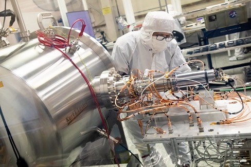
Figure 3. Testing of FM MASPEX instrument.
2.4. Surface Dust Analyzer
The SUrface Dust Analyzer (SUDA) will map the chemical composition of particles ejected from Europa’s surface by hypervelocity impacts of micrometeoroids. The dust particles have a typical size of 0.5−1 μm and exhibit a near isotropic distribution and only weak temporal variations. Small fluctuations are expected from variability of exogenous sources, resulting, e.g., from the orbital motion of sources on Io and the stochastic nature of volcanic activity. SUDA is a time-of-flight mass spectrometer for species with atomic mass ranging of up to 200 u and is capable of detecting up to 40 ejecta per second. Owing to the deterministic nature of the ballistic trajectories of the ejected particles, the composition measurements at spacecraft altitude can be correlated with geologic features on the surface. It has been demonstrated that trace amounts of complex organic species embedded in ice grains with abundances <0.1 ppm can be detected. In addition to micrometeorite ejecta, SUDA will measure the makeup of potential plumes by directly sampling microscopic particles. The FM sensor assembly (Figure 4) will be delivered to ATLO in August 2022 as part of the instrument.

Figure 4. SUDA FM sensor assembly.
3. Mission Concept
The current mission design consists of 49 flybys of Europa executed over a ~3.5 year period while the spacecraft is in orbit about Jupiter. The altitudes of closest approach typically range from 25 km to 100 km. The tour is divided into two principal campaigns, visiting first the anti-Jovian hemisphere followed by observations of the sub-Jovian hemisphere. The flybys occur over a wide range of latitudes and longitudes (Figure 5), and they are widely distributed in true anomaly and solar local time. The tour is thus well suited for characterization of the ice shell and ocean and of the atmosphere and ionosphere created through Europa’s interaction with Jupiter’s magnetosphere.
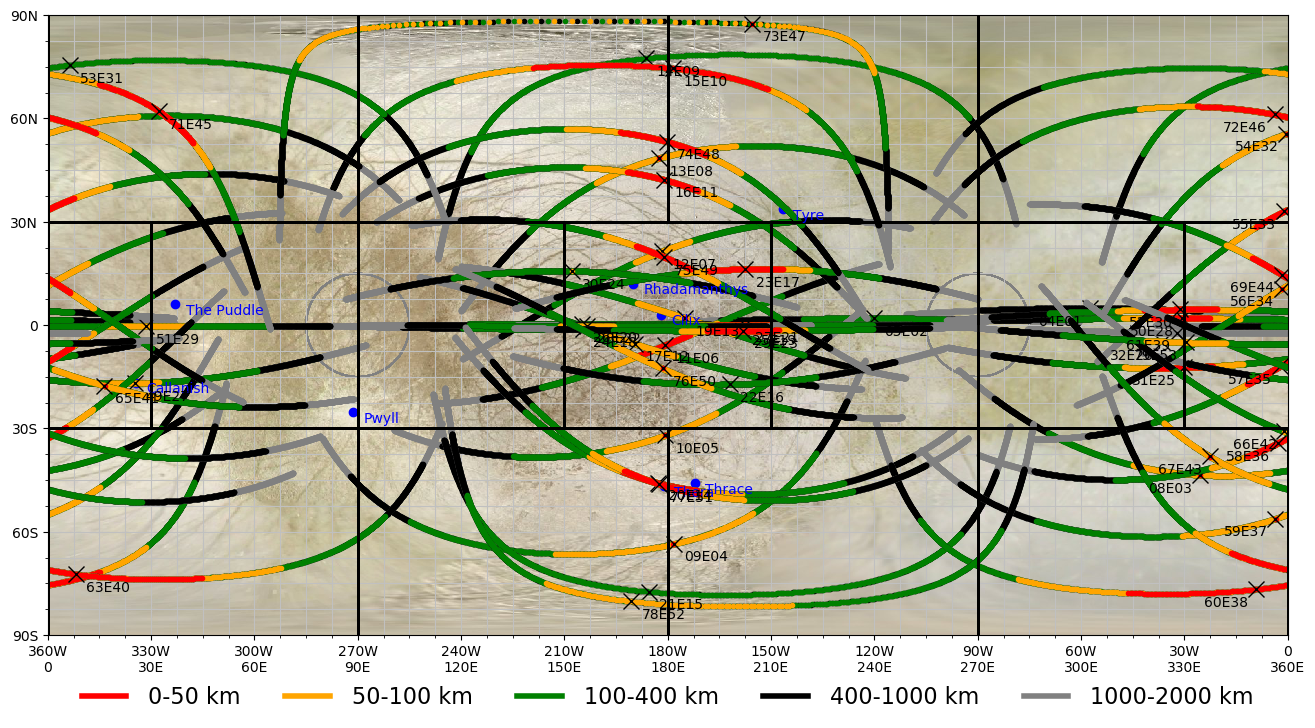
Figure 5. Planned Europa Clipper close approach ground tracks below 1000 km altitude (black), 400 km (green), 100 km yellow, and 50 km (red).
How to cite: Korth, H., Pappalardo, R., Buratti, B., Kempf, S., Kivelson, M., Burch, J., and Westlake, J.: In-situ Investigations of the Europa Clipper Mission, Europlanet Science Congress 2022, Granada, Spain, 18–23 Sep 2022, EPSC2022-429, https://doi.org/10.5194/epsc2022-429, 2022.
The flyby of Pluto by the New Horizons spacecraft in 2015 revealed stricking features in a nitogen ice filled basin named Sputnik Planitia (SP). On the large (few 10 km) scale, irregular polygons [1] have been interpreted as resulting from solid-state convection [2, 3], with down-welling currents at the polygons’ edges [4]. It was first proposed that convection was driven by heating from below, associated with radioactivity in Pluto’s core but it produces a flow that is opposite to the observations with upwelling currents at polygons’ edges [5] (fig. 1a). At the small scale, we can observe pits that have been explained as produced by sublimation of nitrogen ice. The development of this pattern when getting toward the polygons’ sides has been used to estimate the flow velocity on several polygons, of the order 10 cm yr−1 [4]. We proposed [6] that sublimation is also at the origin of convection by cooling the surface: sublimation consumes latent heat which results in the surface of SP being ∼ 5 K colder than the surroundings [7].
We developed a theory to take into account sublimation in a convection model and showed that it leads to a mixed-type (Robin) thermal boundary condition which, in the case of SP is close to that of a fixed temperature. Starting from a uniform temperature in the ice layer, imposing a colder surface value leads to cooling and convection. With the best estimates of the various parameters for SP, a Rayleigh number of order 1 × 10⁵ can be obtained, justifying the possibility of convection. We used a mantle convection model to explore systematically the effect of surface cooling on convection in a temperature-dependent viscosity solid. Depending on the Rayleigh number and the viscosity contrast, we obtain different regimes (fig. 1b), including one with polygons that match the observations of SP (fig. 1c). The five cases that we obtained in that regime can be used to explore the relationships between observed quantities, like the polygonal sizes, and unconstrained ones, like the thickness of the ice layer or the amplitude of topography [6]. Such large-scale dynamics of a solid state layer driven by climate is unprecedented in the knowledge of planetary bodies but might also operate on other volatile rich moons and TNOs.
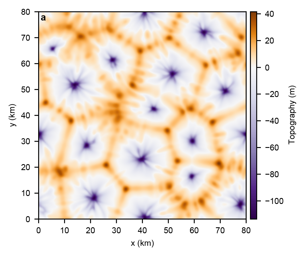

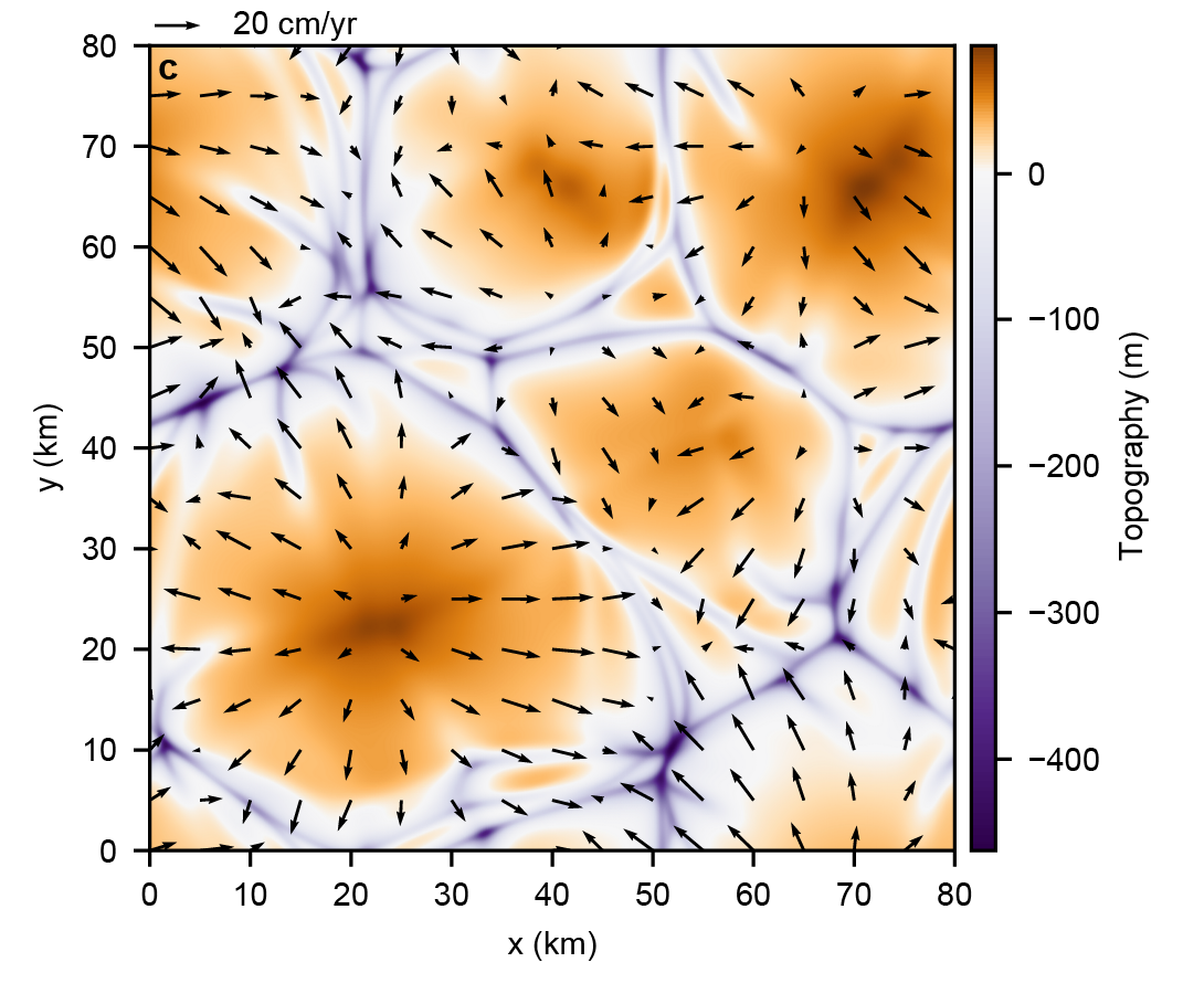
Figure 1: Convection pattern for bottom heated convection (a), convection driven by sublima- tion at the surface (c) and regime diagram as function of the Rayleigh number and viscosity contrast (b).
References: 1. White, O. L. et al. Icarus 287 (2017). 2. Trowbridge, A. J., Melosh, H. J., Steckloff, J. K. & Freed, A. M. Nature 534 (2016). 3. McKinnon, W. B. et al. Nature 537 (2016). 4. Buhler, P. B. & Ingersoll, A. P. Icarus 300 (2018). 5. Vilella, K. & Deschamps, F. J. Geophys. Res. 122 (2017). 6. Morison, A., Labrosse, S. & Choblet, G. Sublimation-driven convection in Sputnik Planitia on Pluto. Nature 600 (2021). 7. Gladstone, G. R. et al. Science 351 (2016).
How to cite: Morison, A., Labrosse, A., and Choblet, G.: Sublimation driven convection in Sputnik Planitia on Pluto, Europlanet Science Congress 2022, Granada, Spain, 18–23 Sep 2022, EPSC2022-434, https://doi.org/10.5194/epsc2022-434, 2022.
UP-FRONT SUMMARY
Canonically, researchers explore the outermost viscoelastic shells of the Galilean satellites as the layers primarily responsible for the diurnal dissipation of gravitational potential energy stored within their eccentric orbits around Jupiter. In this study, we find that tidal heating within solid, inner iron cores may be a first-order control on the heat budget of the resonant Galilean satellites.
This has widespread implications for body evolution, sustained geologic activity within the core and rocky mantles of these worlds, episodic resurfacing, magmatism, and their future exploration. Understanding the role of metallic core dissipation is key to understanding the habitability of Europa and Ganymede, the potential for a magma ocean on Io, and the history of Callisto. Future measurements by NASA’s Europa Clipper and ESA’s JUICE spacecraft will help to unravel the contributions of core dissipation to these global heat budgets.
DISSIPATIVE CORE PLAUSIBILITY
Observations of Io indicate a metal-rich core (e.g. Van Hoolst et al., 2020). At Europa, Schubert et al. (2009) infer that a metallic core is both permitted and likely, though a core is not uniquely required (Bills et al., 2009). Ganymede’s intrinsic magnetic field provides strong evidence for a metallic core (Schubert et al., 1996). Callisto, however, is likely only partially differentiated, with a dense rocky/metal core and a lighter silicate mantle (e.g. Bagenal et al., 2007). Figure 1 shows constraints on core state for Europa.
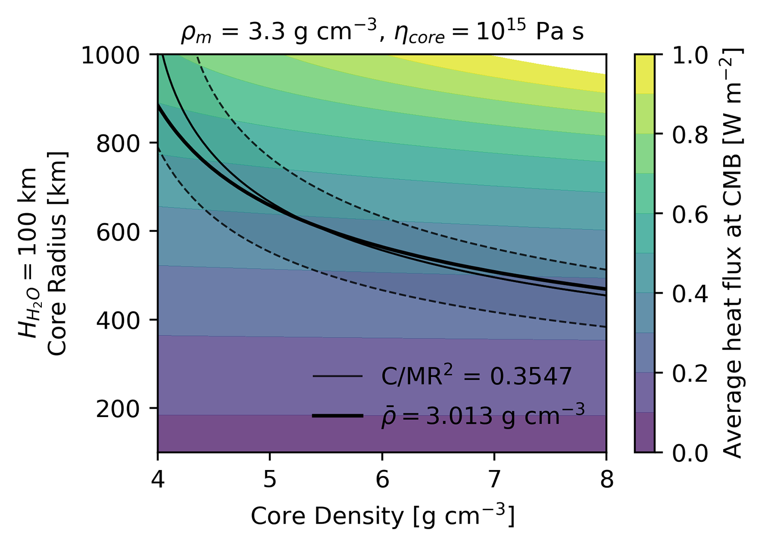
Figure 1: For an example Europa, Bulk density (thick) and Moment of Inertia (thin, dashed) constraints (Casajus et al., 2020). Colors show tidal heat flux at the CMB due to only core dissipation.
On Earth, there is a high plausibility that the solid inner core exhibits viscosities ranging from ~1013–1018 Pa s (Ritterbex and Tsuchiya, 2020), reflecting seismic (1013 Pa s), geodynamic (< 1016 Pa s; Buffett, 1997), and orbital constraints (~1013–1014 Pa s; Koot and Dumberry, 2011).
For the range of iron shear moduli applicable to the Galilean cores (~15–45 GPa; Birch, 1952), the viscosities that maximize dissipation are of the order ~1014–1016 Pa s. Newtonian creep likely dominates at the low pressures of the Galilean satellites cores (Van Orman, 2004), and pure iron viscosities (Birch, 1952) are in the range of 1010–1020 Pa s, depending on temperature and grain size (Figure 2).
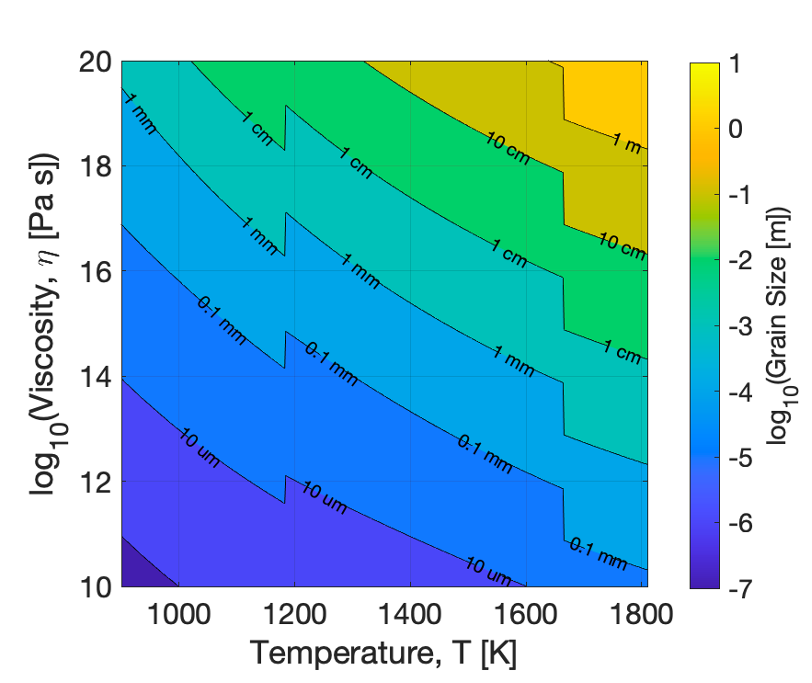
Figure 2: Pure iron rheology (Birch, 1952) as a function of temperature and grain size.
We estimate dissipated power from the tidal response of Io, Europa, and Ganymede using a Maxwell rheology (Figure 3). We find that core dissipation at Io and Europa can exceed that of their outer viscoelastic layers. At Ganymede, the heat flux contribution from the iron core is less than the radiogenic contribution. However, concentrated at the core-mantle boundary, the heat flux is likely sufficient to sustain continued or episodic melting of the metallic core.
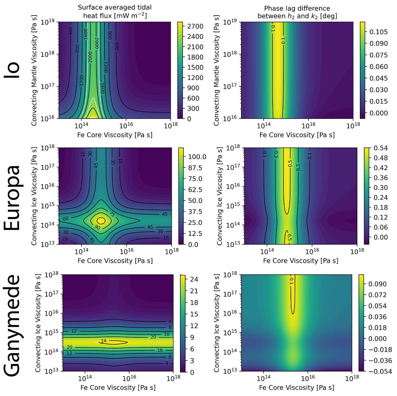
Figure 3: (Left) contours of surface-averaged tidal heat flux as a function of layer viscosity. For Io, white lines indicate constraints from observed dissipation (Lainey et al., 2009). (Right) Phase lag offset between h2 and k2.
ADDRESSING MYSTERIES / SEARCHING FOR ANSWERS
Io’s Magma Ocean: To match observed dissipation, Io’s average mantle viscosity should be ~1014–1013 Pa s (Segatz et al. 1988). However, these values are many orders of magnitude lower than the lowest inferred for Earth’s partially molten asthenosphere (~1019 Pa s; e.g. Dixon et al., 2004) and cannot support the mantle convection associated with high magma eruption temperatures (Moore et al., 2003). The presence of a pervasive “magma ocean” has been proposed to explain discrepancies (e.g. Khurana et al., 2011).
If Io experiences significant core heating, then a rock viscosity consistent with that of Earth’s mantle (1019 Pa s) and core viscosity of ~1015 Pa s can explain the observed heat flux without requiring a magma ocean or low-viscosity mantle (Figure 3).
Periodic Resurfacing and Dynamos at Europa and Ganymede: Europa’s young surface and Ganymede’s terrain dichotomy reflect episodic resurfacing. While dissipation within ice shell would allow rapid changes within those layers, heat conductively diffuses from the core slowly (~100–101 Gyr). Rapid transport may occur through solid-state mantle convection and/or rock melting and ascent from the CMB (Figure 4). Additionally, core melting causes the tidal response to decouple from the solid body (Henning and Hurford, 2014), decimating dissipation.
The timescales for core melting and freezing, the onset and cessation of thermal convection, and the onset and ascent of melting at depth may compete to create an episodicity in seafloor heat flux, and may modulate the response to episodic changes to the orbital configurations of the satellites. Changes in heat flux may drive resurfacing through induced changes in the ice shell thickness and geodynamic state (Nimmo, 2004), and rotational coupling to the interior.
Callisto’s lack of evidence for resurfacing and sustained (un-forced) orbital eccentricity may reflect the absence of a dissipative iron core, and inefficiency of icy dissipation within the satellite.
Observational Predictions: If core dissipation is meaningful today, it may be observable in the phase lag difference between k2and h2 (Figure 1). In the absence of a phase lag offset, we predict that the present-day core may be partially molten, decoupling it from the solid body and decreasing dissipation, potentially producing an intrinsic magnetic field. If an iron core is responsible for Io’s observed high heat flux, we expect the real part of k2 to reflect a solid body (~0.09) rather than a body with an internal fluid layer (~0.5) per Bierson and Nimmo (2016).
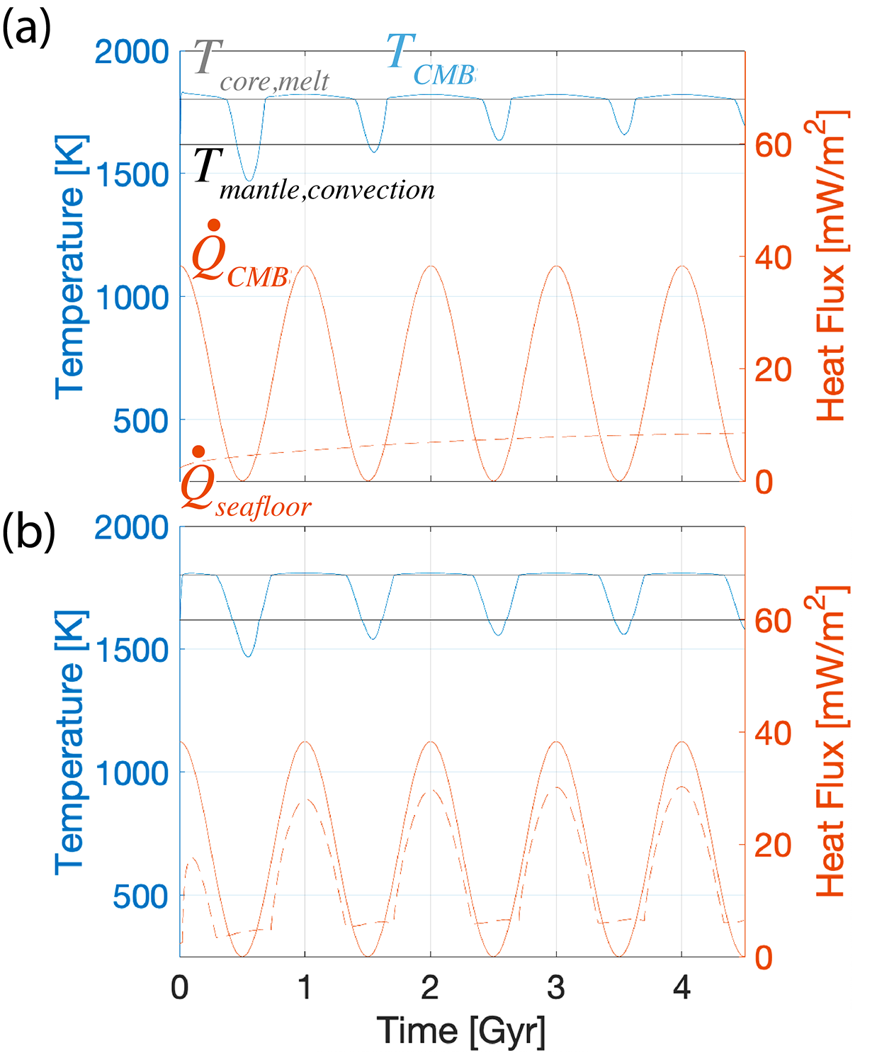
Figure 4: Europa’s (surface-averaged) seafloor heat flux (orange dashed line) responds to periodic changes in core dissipation (solid orange line). CMB temperatures (blue) vary from melting across the critical temperature for mantle convection. Heat transfer occurs through (a) diffusion, and (b) self-consistent melt migration and convection.
ACKNOWLEDGEMENTS
This work was performed at the Jet Propulsion Laboratory, California Institute of Technology, under contract with NASA, and supported through the NASA Habitable Worlds (80NM0018D0004), the Europa Clipper project, and the NASA Postdoctoral Program, administered by Oak Ridge Associated Universities under a contract with NASA (80HQTR21CA005).
How to cite: Howell, S., Vance, S., Bills, B., Melwani Daswani, M., Styczinski, M., and Hay, H.: Powering fire and ice with iron: Strong metallic core dissipation within the Galilean satellites, Europlanet Science Congress 2022, Granada, Spain, 18–23 Sep 2022, EPSC2022-729, https://doi.org/10.5194/epsc2022-729, 2022.
Models for the internal structure of the icy satellites Ganymede and Titan, as derived from the data of the Galileo and Cassini-Huygens space missions, suggest that both moons are differentiated with a hydrosphere of ices and liquid water overlaying an inner rocky core. The presence of significant amounts of Insoluble Organic Matter (IOM) in this silicate layer (in quantities consistent with those found in chondrites) has recently been advanced to properly explain the density and moment of inertia of these moons [1]. Interestingly, laboratory experiments at room pressure have shown that the pyrolysis of IOM (starting from temperatures as low as 500 K) gradually releases volatiles such as H2O, CO/CO2, CH4, H2S, and SO2, with possible N-bearing compounds such as N2, NOx and NH3 [2, 3, 4]. This evolution of the IOM could have a defining impact on the habitability and chemical evolution of icy worlds, including the formation of an atmosphere. However, the effect on these thermal reactions of the high pressures found inside large icy worlds remain largely unknown. The purpose of this study is to analyze the chemical and physical evolution of the IOM under the combined pressure and temperature conditions expected inside Titan and Ganymede (pressures from 0.5 to 7 GPa and temperatures up to 1200 K).

Figure 1: Species produced by IOM dissociation at high pressure and high temperature (blue) compared to those produced by pyrolysis at ambient pressure in Kuga et al. (2014) (green) and Okumura and Mimura (2011) (red).
We conducted anvil cell experiments on mixtures of IOM with water at temperatures up to 773 K and pressure up to 8 GPa. The IOM, with a composition of C100H93N65O61, was synthetized at the Nebulotron (CRPG, France [3]), an ultra-high vacuum chamber using a radiofrequency plasma to ionize a N2-CO gas mixture. Systematic pressure and temperature monitoring, and in situ Raman spectroscopy analyses, were conducted during the experiments to characterize the evolution of the samples. Additional infrared analyses were conducted to compare the initial organic matter (as loaded in the anvil cell) with the residual IOM collected at the end of some of the experiments.
During our high-pressure experiments, elevated temperatures led to the production of C- and N-bearing species, as was reported by others during the pyrolysis of dry IOM at room pressure. Our IOM-water mixtures, however, yielded NH3 (rather than N2) as the main N-bearing molecule. Furthermore, CO2 was never observed in our samples; instead, CO3 (as carbonic acid and/or carbonate ions) was identified as the main C-bearing species alongside CH4 (Figure 1). Overall, the degradation of the IOM at high pressure appears to start at slightly higher temperature, although additional experiments are needed to confirm this result (in particular for the formation of CO3 species). Evidence of the restructuration of the IOM appeared in both Raman and infrared spectroscopy.
Our results support that the thermal dissociation of the IOM inside Titan may have contributed to the formation of its atmosphere [5,6]. These results will also prove useful in assessing the chemical evolution of the hydrosphere of icy worlds, notably regarding the formation of gas hydrates inside their high-pressure ice layers.
Acknowledgements:
This research is founded by CNRS 80 PRIME program. This work also acknowledges the financial support from CNES (Centre National d’Etudes Spatiales, France) in preparation of the ESA JUICE mission.
References:
[1] Néri et al. (2020) A carbonaceous chondrite and cometary origin for icy moons of Jupiter and Saturn. Earth and Planetary Science Letters, 530 :115920.
[2] Okumura and Mimura (2011) Gradual and stepwise pyrolysis of insoluble organic matter from the Murchison meteorite revealing chemical structure and isotopic distribution. Geochimica et Cosmochimica Acta, 75(22) :7063–7080.
[3] Kuga et al. (2014) Nitrogen isotopic fractionation during abiotic synthesis of organic solid particles. Earth and Planetary Science Letters, 393:2–13.
[4] Franklin (1949) A study of the fine structure of carbonaceous solids by measurements of true and apparent densities. Part I. Coals. Transactions of the Faraday society, 45:274–286.
[5] Tobie et al. (2012) Titan’s bulk composition constrained by Cassini-Huygens: implication for internal outgassing. The Astrophysical Journal, 752(2):125.
[6] Miller et al. (2019) Contributions from accreted organics to Titan’s atmosphere: new insights from cometary and chondritic data. The Astrophysical Journal, 871(1):59.
How to cite: Lévêque, P., Sotin, C., Bujoli, B., Bollengier, O., Queffelec, C., Le Menn, E., Clouet, A., Marrocchi, Y., and Tobie, G.: Evolution of Insoluble Organic Matter and H2O mixtures Under Ganymede and Titan’s Interior Conditions, Europlanet Science Congress 2022, Granada, Spain, 18–23 Sep 2022, EPSC2022-792, https://doi.org/10.5194/epsc2022-792, 2022.
Galileo Regio is a dark terrain of Ganymede extending approximately from 180°-120° W to 0°-60° N that shows high crater density and morphotectonic structures called furrows. Such structures are kilometric-scale brittle troughs bounded by high albedo rims and a low albedo floor, and arranged with circumferential and radial setting at the regional scale [1]. Furrows are generally interpreted as the remnants of a multi-ring impact basin similar to the Valhalla basin on Callisto [2]. Galileo Regio shows two main settings of the furrows, which allow their classification into two systems: the concentric furrows of Lakhmu Fossae system, which is crosscut by the radial furrows of the Zu Fossae system [3]. In addition, Galileo Regio shows local-scale structures that rework the pristine morphology of the Lakhmu Fossae furrows.
In this contribution, we investigate the furrows of Galileo Regio at both regional- and local-scale to unravel the tectonic evolution of the dark terrain. We perform a structural mapping and geostatistical analyses of the furrows in Galileo Regio, identifying their hierarchy and tectonic setting originated by regional-scale kinematics. Structure attributes such as structure length, sinuosity, azimuth, spacing within the adjacent structures, have been quantitatively characterized and allow to perform the azimuthal distribution, the Length/Spacing [5] and the paleo-stress analyses [6]. Such analyses allow to identify the structural systems and to infer the past stress fields that affected Galileo Regio (maximum and minimum horizontal stress, i.e., SHmax and Shmin, respectively). A total of four structural systems have been recognized within Galileo Regio: i) the already known Lakhmu and Zu Fossae; and ii) the Lineated system and Precursor system, proposed by this work for the first time (Fig. 1).
Such systems are the result of phases of the tectonic activity that affected Galileo Regio during the geologic history of Ganymede. We identify the sequence of such phases that allow to produce an evolutionary tectonic model (Fig. 2): i) t0 represents a NW-SE extension that formed the Lineated system; ii) t1 represents the impact that originated a multi-ring basin [3, 7], i.e., the Lakhmu Fossae; iii) t2 shows the extensional activity responsible for the formation of the light terrain of Uruk Sulcus [8] and for the formation of the extensional structures of the Precursor system; iv) t3 represents the kinematics consistent with the right-lateral transpression that has affected Uruk Sulcus [4] and formed the Zu Fossae; and v) t4 presents a right-lateral strike-slip that contributes to the formation of the Precursor system.
The obtained results and the presented model will be used for the scientific preparation of dedicated high-resolution observations that will be taken with the JANUS instrument [9] onboard the JUICE mission [10].
Acknowledgments: The activity has been realized under the ASI-INAF contract 2018-25-HH.0.
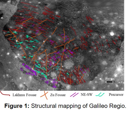
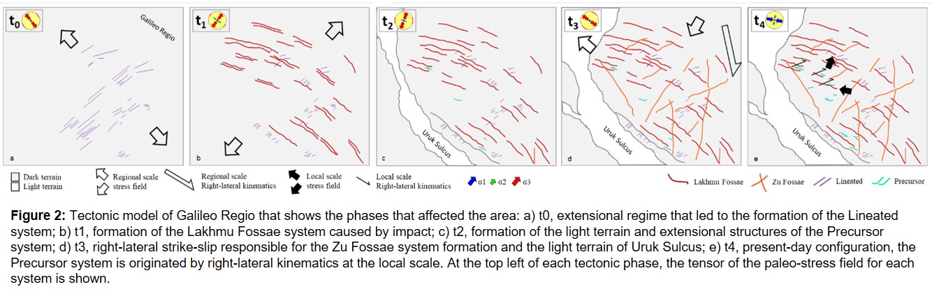
References:
[1] Patterson, W. et al. (2010). Icarus 207,845–867; [2] McKinnon, W.B. and Melosh, H.J. (1980). Icarus 44 (2), 454–471; [3] Prockter, L.M., et al. (2000). Journal of Geophysical Research: Planets, 105(E9), 22519-22540; [4] Kersten, E., et al. (2021). Planetary and Space Science, 206, 105310; [5] Rossi, C., et al. (2018). Tectonophysics 749, 72–87; [5] Delvaux, D., and Sperner, B. (2003). Geol. Soc., London, Special Publications, 212(1), 75-100; [7] Hirata, N., et al. (2020). Icarus, 352, 113941; [8] Pappalardo, R.T., et al. (1998). Icarus, 135(1), 276-302; [9] Palumbo, P., et al. (2014). 45th LPSC Meeting. Abstract #2094; [10] Grasset, O., et al. (2013). Planetary and Space Science, 78, 1–21.
How to cite: Rossi, C., Lucchetti, A., Massironi, M., Pozzobon, R., Penasa, L., Munaretto, G., and Pajola, M.: Structural evolution of Galileo Regio, dark terrain of Ganymede., Europlanet Science Congress 2022, Granada, Spain, 18–23 Sep 2022, EPSC2022-815, https://doi.org/10.5194/epsc2022-815, 2022.
Introduction : Europa’s surface is one of the youngest surfaces in the solar system. The great diversity of morphologies observed quickly raised the question of the processes responsible for this active resurfacing. The Jovian moon is believed to hide a global liquid water ocean under its ice crust [1] which led to the assumptions of exchange between the surface and the putative subsurface ocean [1]. In addition, Europa is exposed to intense space weathering due to the continuous bombardment by electrons and ions from Jupiter’s magnetosphere [2]. The surface therefore appears as the key witness of these internal and external processes.
To finely characterize the microphysics of the ice it is necessary to use radiative transfer (RT) modeling. Such modeling allows to estimate these parameters integrating the highly nonlinear effects of the light path within the icy regolith due to scattering. A recent work has been proposed to determine surface properties using Bayesian Monte Carlo Markov Chain (MCMC) [3]. This approach is based on RT models [4,5] using the optical properties of the considered chemical species and physical properties of the regolith. Here we report the use of a RT model [5] in a Bayesian MCMC inference framework to retrieve microphysical properties of Europa's surface using the Galileo Near-Infrared Mapping Spectrometer (NIMS) hyperspectral data [6].
Data: We use data acquired by NIMS collected during the Galileo mission. Here we present the analysis of calibrated data from the hyperspectral cube "e6007ci" (available from the PDS archive) from the trailing Anti-jovian hemisphere (Fig. 1). The estimated signal-to-noise ratio (SNR) is between 5 and 50, we mainly focus on the 1.0-2.5 µm region for which the SNR is higher. Within this spectral range the uncertainty on the absolute calibration is up to 10% [7].
Radiative transfer model requires the optical constants of the pure chemical species considered. Here we consider 15 different compounds: crystalline and amorphous water ice [7,8], sulfuric acid octahydrate (SAO; [2]), hydrated sulfates [9,10], hydrated chlorine salts [11], and minerals such as magnetite [12], sodium chloride [13] and ammonium sulfate [14].
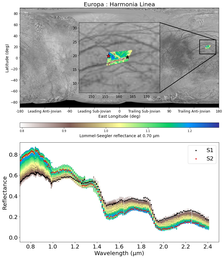
Figure 1 - (top): Map of Europa with a zoom on Harmonia Linea observation. The color represents the reflectance at 0.7 µm normalized using the Lommel-Seegler law. (bottom): all spectra from the corresponding cube and the selected spectra (S1 and S2) used in this study.
Method: We use a MCMC Bayesian inference approach [15,16] to analyze NIMS spectra because it has the advantage of allowing the exploration of a large parameter space and looking for non-unique solutions while statistically constraining the model parameters [17,18]. We compute the bidirectional reflectance of the regolith using a RT model [5]. Then, the algorithm is used to sample the parameter space following the Bayesian Posterior distribution. The parameters we are adjusting are: abundances, grain size of each chemical species and macroscopic roughness of the regolith. For the abundances we use a Dirichlet prior to ensure that they are sum up to 1, while we use a uniform distribution prior for the other parameters.
A first study was done to test all combination of 3, 4 and 5 chemical species among the 15 compounds on the S1 spectrum to select the most appropriate chemical species to consider for the surface characterization. For each of this combination (4823 in total), we perform the MCMC inversion.
Results: We first discuss the chemical species selection (called here endmember) by looking at all best-fit from all combination of 3, 4 and 5 endmembers and their associated RMS. We first show that going from 3 to 4 endmembers significantly improves the quality of the fit while using 5 endmembers only slightly improve it. In addition, some compounds appear necessary to reproduce the observation, such as water ice and SAO. We show that adding either hydrated sulfates or chlorine salts produces results substantially similar. Fig. 2 illustrates such results when considering 4 endmembers. Finally we perform MCMC inversion with 5 endmembers including both crystalline and amorphous water ice. The best fit from the 5 endmembers model and their associated posterior pairwise distribution are shown fig. 3 and 4 for the S1 and S2 spectra.
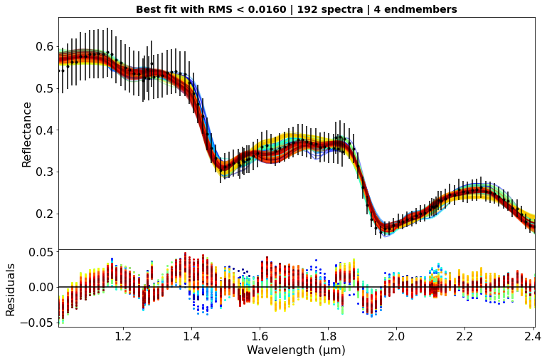
Figure 2 - Results of all combination for the 4 endmembers case: only the best-fit with RMS below 0.016 are showed.
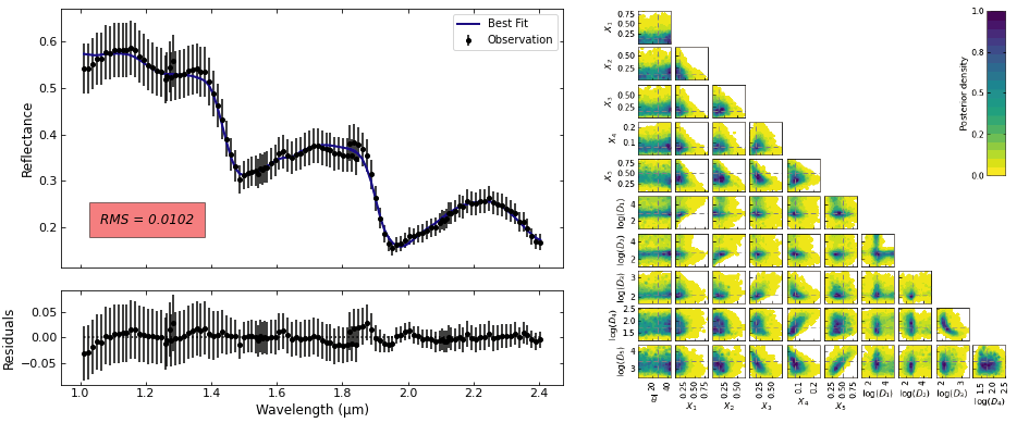
Figure 3 - results for S1: best fit (left) and pairwise posterior distribution (right) using 5 endmembers.
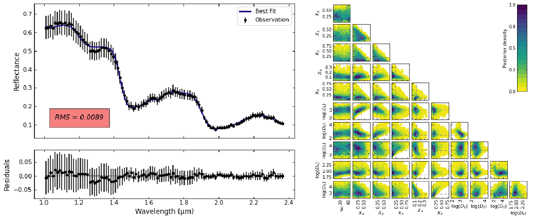
Figure 4 - results for S2: best fit (left) and pairwise posterior distribution (right) using 5 endmembers.
Conclusion: We tested, for the first time and in a systematic way, the inversion of Galileo NIMS infrared spectra using a significant number of 3, 4 and 5 compounds combinations out of a selection of 15 chemical compounds, using a non-linear radiative transfer model. We found that there is no unique solution to determine the exact composition of the surface, but a family of endmember are required: water ice, SAO and sulfates. This composition set seems to be coherent for both bright and dark regions of Europa. We will discuss the implication of these results on the Europa’s surface processes.
References: [1] Pappalardo, R. et al. (1999) JGR. [2] Carlson, R. W. et al. (2005) Icar. [3] Mishra, I. et al. (2021) Planet. Sci. [4] Hapke, B. (2012). Cambridge Univ. Press. [5] Douté. S. and Schmitt. B. (1998) JGR. [6] Carlson, R. et al. (1992) ed. C. T. Russell. [7] Schmitt, B. et al. (2004). [8] Trotta, F and Schmitt, B (2018). [9] Dalton, J.B. et al. (2012) JGRE. [10] D. Angelis, S et al. (2021) Icar.. [11] Hanley, J. et al. (2014), JGR. [12] Roush, T. et al. (2021) Icar. [13] Querry, M. (1987). [14] Fastelli, M. et al. (2022), Icar. [15] Cubillos, P. et al. (2016), The Astr. Jour. [16] Braak, C. J. F. (2008), Stat & Comp. [17] Mosegaard, K. et al. (1995) JGR. [18] Schmidt, F. and Bourguignon, S. (2019) Icar.
How to cite: Cruz Mermy, G., Schmidt, F., Andrieu, F., Belgacem, I., Cornet, T., and Altobelli, N.: New insights into Europa's surface using Galileo/NIMS data and MCMC modeling, Europlanet Science Congress 2022, Granada, Spain, 18–23 Sep 2022, EPSC2022-825, https://doi.org/10.5194/epsc2022-825, 2022.
Events which deposit fresh material onto Europa’s surface may be irregular and catastrophic, such as large-scale impacts, or localized, and potentially extant, processes in which faults, fractures, or brine transport bring subsurface liquid onto the surface. This liquid may originate from shallow reservoirs within the ice shell or directly from the subsurface ocean [1]. Emplacement may be a slow, extrusive process, or quicker, potentially with the formation of cryovolcanic plumes (e.g. [2,3,4]). Plume deposits or any other surface material can also be transported to high altitudes by another mechanism: when hypervelocity interplanetary micrometeoroids, or larger objects, impact the surface of an atmosphereless planetary body like Europa, these can generate impact ejecta with high enough velocities to reach altitudes of hundreds of kilometres [5]. Most of these ejecta particles are gravitationally bound, moving on ballistic trajectories lasting up to hundreds of seconds and producing an almost isotropic dust exosphere around Europa [6,7]. Subsurface oceans, in the Jovian and in other planetary systems, can therefore be characterized using the particles they emit, via either indirect or direct routes: 1) Detection and analysis of ejecta particles lofted by micrometeoroid impacts from those parts of the surface that recently interacted with subsurface water (e.g. certain landforms, such as chaos terrains on Europa, or plume deposits); 2) Direct sampling of plume particles in space (where plumes are present, as perhaps possible on Europa).
The SUrface Dust Analyzer (SUDA), onboard the Europa Clipper spacecraft, is designed to measure the composition and trajectories of such impact ejecta particles and/or plume material. SUDA is an impact ionisation time-of-flight mass spectrometer, which uses the ions generated by hypervelocity impacts of dust grains onto the instrument target to generate mass spectra of the impinging particles. Depending on the altitude, SUDA will be able to detect up to tens of ejected surface particles per second during each flyby, each likely to contain a wide variety of organic and/or inorganic compounds, and via trajectory reconstruction, map them to their origins on the surface [8].
At global scales, landform evolution on atmosphereless bodies is primarily driven by impact gardening and tectonics. The tectonic regime that dominates within Europa’s ice shell is likely to be extensional, a hypothesis supported by numerous lines of evidence, such as the widespread presence of dilational bands that represent >40% of the total surface area [9]. Several types of geological features generated within such a tectonic regime, including chaos terrains and fossae, might affect the emplacement of buried material and subsequent exposure of fresh volatiles on Europa’s surface.
Chaos Terrains are, on Europa, geologically very young and extensively disrupted surface features, interpreted as reflecting recent interaction with subsurface material [10]. Leading-hemisphere chaos regions have recently been shown to be compositionally distinct from their surroundings, probably indicating contributions from endogenous sodium chloride sourced from the subsurface ocean [11,12]. Fossae are long, narrow depressions (troughs). The term is used for topographic features that occur on extraterrestrial planetary surfaces, whose exact origin is uncertain, although they are thought to be the result of extensional tectonic processes [13].
Here we investigate two neighboring features on Europa, Ménec Fossae and Thrace Macula (a chaos terrain), for which we produced high-resolution photoclinometrically-derived [14] digital terrain models (DTMs, Fig. 1) and geomorphological-structural maps (Fig. 2). Our preliminary results suggest that this area of Europa has undergone transtensional (strike-slip paired with extension) tectonic activity, as indicated by the orientation and relationship of the faults and fossae. Such tectonic style has possibly created a pathway facilitating the ascent of subsurface material, especially volatiles, that play an important role in the formation of chaos terrain. These results will help ascertain the most likely regions on Europa in which to find fresh material, representative of the subsurface ocean, and be used as input data for dust ejecta trajectory models that will ultimately assist the mass spectrometer Surface Dust Analyzer (SUDA), onboard the upcoming Europa Clipper mission, in compositionally mapping Europa’s surface [15].
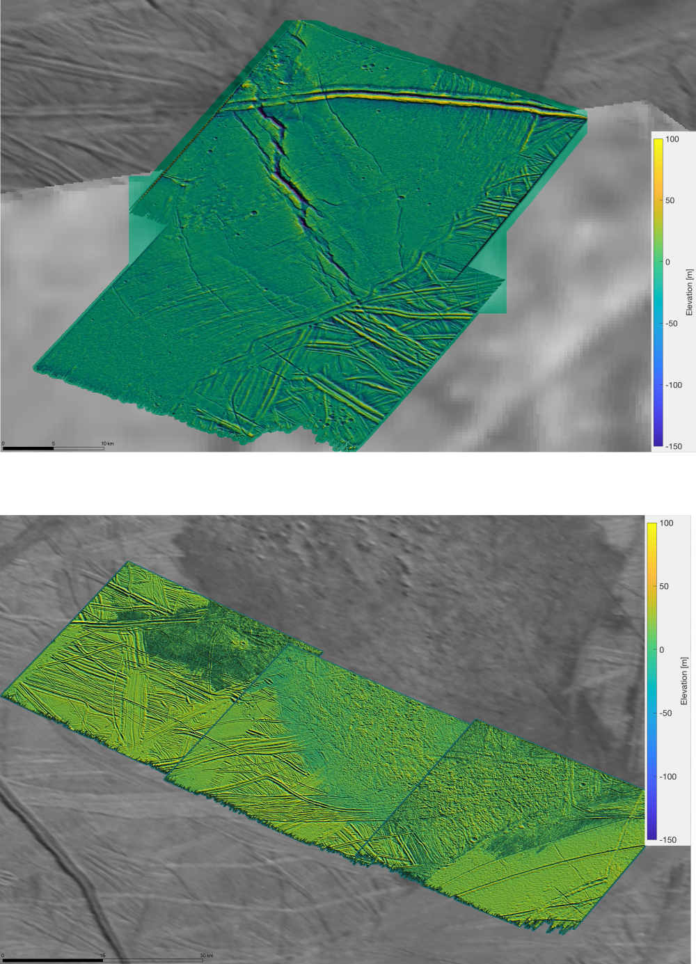
Figure 1. Regional DTMs, Ménec Fossae (top) and Thrace Macula (bottom)
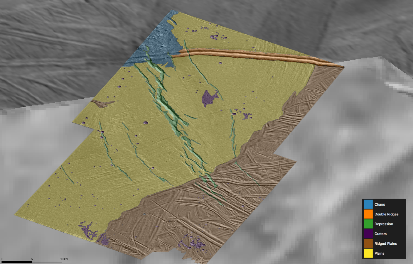
Figure 2. Geomorphological map of Ménec Fossae
- 1. Head, J.W., & Pappalardo, R.T., (1999). J. Geophys. Res. 104, 27143–27155.
- 2. Roth, L., et al., (2014). Science 343, 171.
- 3. Sparks, W.B., et al., (2017). The Astrophysical Journal Letters, 839(2), L18.
- 4. Jia, X., et al., (2018). Nat. Astron. 2, 459.
- 5. Koschny, D., & Grün, E., (2001). Icarus, 154(2), 402-411.
- 6. Krivov, A. V., et al., (2003a). Planetary and Space Science 51, 251-269.
- 7. Postberg, F., et al., (2011). Planetary and Space Science, 59(14), 1815–1825.
- 8. Goode, W., et al., (2021). Planetary and Space Science, 208, 105343
- 9. Kattenhorn, S.A. & Hurford, T.A., (2009). In: Europa, 199-236.
- 10. Schmidt, B. E., et al., (2011). Nature 502, v. 479
- 11. Trumbo, S. K., et al., (2019). SciA, 5, aaw7123
- 12. Trumbo, S. K., et al., (2022), PSJ, 3, 27
- 13. Schenk, P., et al., (2020). Geophys. Res. Let., 47, e2020GL088364
- 14. Lesage et al., (2021). Icarus, Volume 361, 114373.
- 15. Kempf, S., et al., (2019). AGU Fall Meeting 2019, abstract #P53D-3500
How to cite: Matteoni, P., Neesemann, A., Schmidt, J., Hillier, J., and Postberg, F.: Geomorphology and topography of Ménec Fossae and Thrace Macula on Europa: Insights on formation processes, Europlanet Science Congress 2022, Granada, Spain, 18–23 Sep 2022, EPSC2022-914, https://doi.org/10.5194/epsc2022-914, 2022.
Introduction
Tidal dissipation is an important source of heat for several icy moons of Jupiter and Saturn. While the evaluation of tidal heating in the solid parts of the moons is straightforward, with the only limitation being the lack of knowledge about anelastic properties of ice and silicates, modeling the tidal dissipation in subsurface oceans is challenging and the issue of how much it contributes to the total heat production has not yet been fully resolved. The standard approach to modeling the tidal dissipation in a subsurface ocean is based on the solution of hydrodynamic equations in the shallow water approximation [e.g., 1– 4]. Numerical studies addressing the tidal deformation of the ocean in a three-dimensional geometry have appeared only recently [5,6]. Although these studies represent significant progress, they have one important limitation: they do not take into account the mechanical coupling between the flow in the ocean and the viscoelastic deformation of the ice shell and the core. To overcome this limitation, we have developed a new method that allows the tidal deformation to be solved simultaneously in all three parts of the icy moon.
Method
The problem of tidal deformation is solved in a spherical computational domain corresponding in size to Saturn’s moon Enceladus and consisting of three sub-domains (the viscoelastic ice shell, the viscous ocean, and the viscoelastic core), which are coupled by the boundary conditions. The Navier-Stokes equation is integrated in time and solved using a pseudo-spectral method based on spectral decomposition in angular coordinates and finite differences in radius. The spherical harmonic coefficients are discretized in 800 unevenly spaced grid points guaranteeing a sufficiently high sampling density in the boundary layers. Self-gravitation and the Coriolis force are included. The thickness of the ocean is varied from 10 m to about 50 km and its viscosity is considered in the range 1–106 Pa s. Calculations are performed for two end-member cases, recently discussed in literature: a weakly deformable elastic core and a highly deformable Maxwell viscoelastic core [7].
Results and Conclusion
Our results confirm the conclusions of previous studies that tidal dissipation in the present day ocean on Enceladus is negligible compared to the expected heat production [e.g., 8]. However, unlike some previous models, we find less pronounced resonance peaks, suggesting that the mechanical coupling between the ocean and the solid parts of the moon tends to reduce the resonance effects. Our results indicate that dissipation in the ocean strongly depends on the ocean thickness, reaching the maximum value for a thickness of 1 km when the ocean viscosity is 106 Pa s and less than 0.1 km when the viscosity is smaller 10 Pa s. The maximum dissipation predicted in the ocean (1 GW for the weakly deformable core and 20 GW for the highly deformable core) is independent of the viscosity prescribed in the ocean. This suggests that although the tidal dissipation currently plays a negligible role in Enceladus’ heat budget, it can effectively hinder the freezing of the ocean when the ocean is thin.
References
[1] Tyler, 2011, Icarus 211, 770–779.
[2] Chen et al., 2014, Icarus 229, 11-30.
[3] Matsuyama, 2014, Icarus 242, 11–18.
[4] Hay and Matsuyama, 2019, Icarus 319, 68–85.
[5] Rovira-Navarro et al., 2019, Icarus 321, 126–140.
[6] Rekier et al., 2019, J. Geophys. Res.: Planets 124, 2198–2212.
[7] Choblet et al., Nat. Astr. 1, 841–847.
[8] Čadek et al., Icarus 319, 476–484.
How to cite: Aygün, B. and Čadek, O.: A new approach to modeling the tidal dissipation in subsurface oceans of icy moons of Jupiter and Saturn, Europlanet Science Congress 2022, Granada, Spain, 18–23 Sep 2022, EPSC2022-968, https://doi.org/10.5194/epsc2022-968, 2022.
Introduction
The formation of Ganymede’s light terrain and its possible interaction with a subsurface ocean, have made its investigation one of the top goals of the upcoming JUICE mission [1, 2]. In this study we present a detailed stratigraphic analysis of areas that were observed by the Galileo SSI camera at highest possible spatial resolution (scales of ~11 m/pxl) in order to see what information of the light terrain’s stratigraphic position in Ganymede’s surface evolution can be gained from mapping and crater counting results and to identify what still has to be done in order to prepare for the upcoming JUICE mission.
Study areas
Based on the available data set, we selected four major regions (Region A, B, C and D) that are covered by more than one high-resolution SSI image for our study (Fig. 1): Region A and D from the anti-Jovian hemisphere and Region B and C from sub-Jovian hemisphere. Region A comprises of Byblus Sulcus (G2GSGRVLNS01), Nippur and Philus Sulcus (G2GSNIPPUR01) and the Transitional region (G2GSTRANST01) with the context info provided by the SSI observation G8GSREGCON01. Region B is dominated by Arbela Sulcus (28GSARBELA01+02/ G7GSNICHOL01), Region C is the Harpagia Sulcus region (28GSBRTDRK02, 28GSCALDRA02 and 28GSSMOOTH02) and Region D comprises Erech Sulcus (G8GSERECH01), Mummu and Sippar Sulci (G8GSCALDRA01).
Mapping results
Geologic maps are prepared for the four regions using ArcGIS. The naming/categorization of geological units follows from [4, 5] but are refined and modified wherever necessary (Fig. 2). Among the light terrain units, ls and lg are the most commonly occurring than li.
Stratigraphic correlation:
On the whole, the relative ages from crater density measurements (Fig. 5) follow the mapping results. In brief, in Byblus Sulcus the two light terrain units are of similar age from crater counts while lg3 is younger than lg2 from crosscutting relationships. (Fig. 2). In case of Region B (Arbela Sulcus), we could find that the age relationship of the two light terrain units and two dark terrain units agree with the relative age inferred from crosscutting relationship (Fig. 3a) In more extensively resurfaced areas of the light terrain the situation appears to be more complex. In Region C, the terrain units ls also have comparatively higher age than lg terrain units (Fig. 3b-3d). In Region D the terrain units (Fig. 4) are highly interrupted by the secondary craters formed during the Osiris and Melkart impact events [6].
Discussion
We used two most favored chronology models LDM (Lunar Derived Model by [7]) and JCM (Jupiter Comets Model by [8]) (Fig.6). In general, based on the LDM ages the crater densities point to a relatively high age of the light terrain units not much younger that the ancient dark terrain and could imply a relatively short time period of formation for most of our mapped light terrain units. This relatively high age fits into the theory that the light terrain could have formed as a direct result of internal differentiation followed by a global expansion [9]. On the contrary, the JCM derived ages point to a longer formation period of light terrain units around 2 Ga [9]. While the impact chronology in the Jovian system and of its satellites is still not fully solved, newest results infer that the craters on these bodies were created from members of a collisionally evolved impactor family, similar to those in the inner solar system [10]. This does not straightforwardly support the lunar-derived chronology model (LDM) by [7] but allows to derive a Ganymede-specific crater production function empirically from the lunar one. We used this production function to fit our crater distributions and to derive absolute model ages for both model chronologies [7][8].
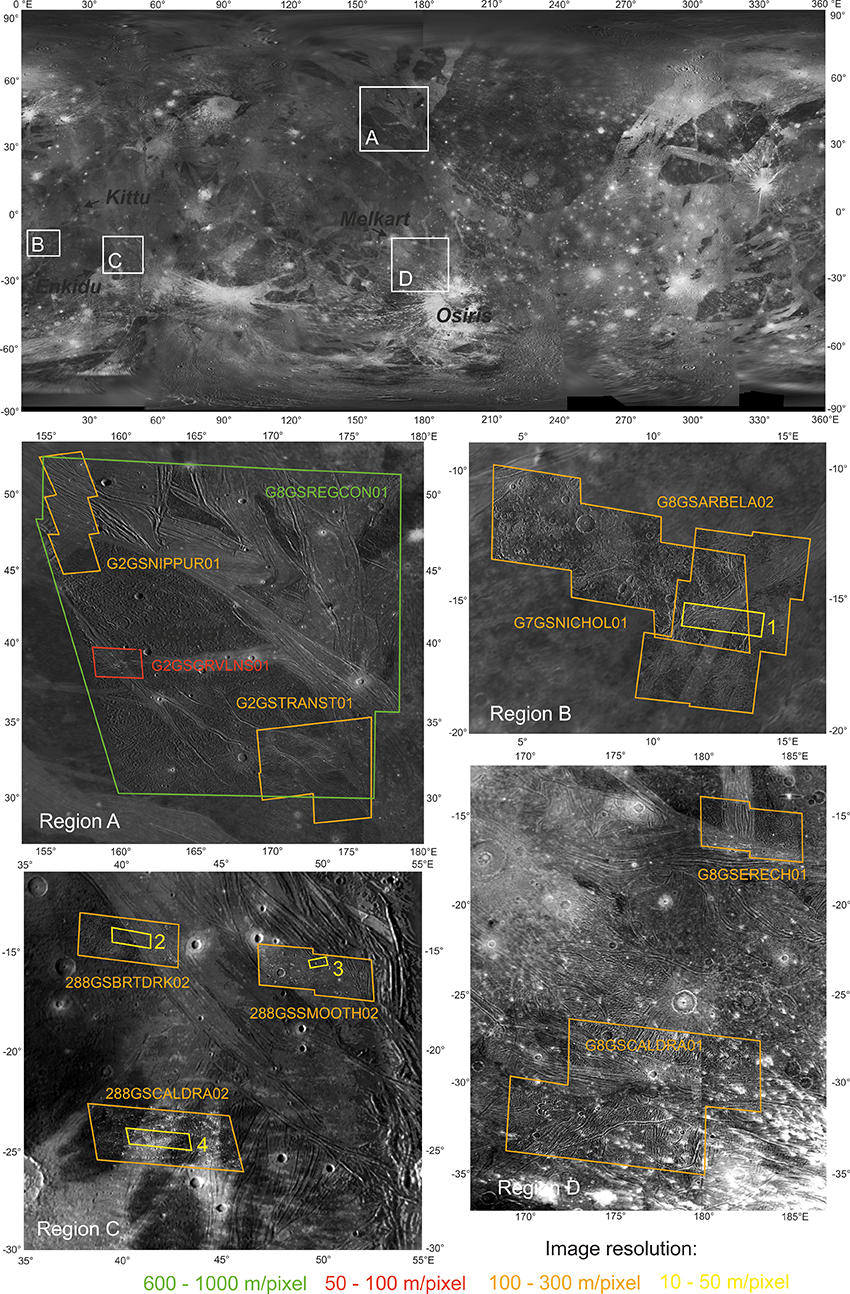
Figure 1: Regions of Interest in this study with the available Galileo SSI coverage indicated.
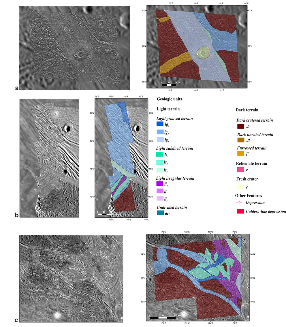
Figure 2: Geologic mapping results for Region A: a) Byblus Sulcus (G2GSGRVLNS01), b) Nippur and Philus Sulcus (G2GSNIPPUR01) and c) the Transitional region (G2TRANST01). The legend applies also to Figures 3 and 4.
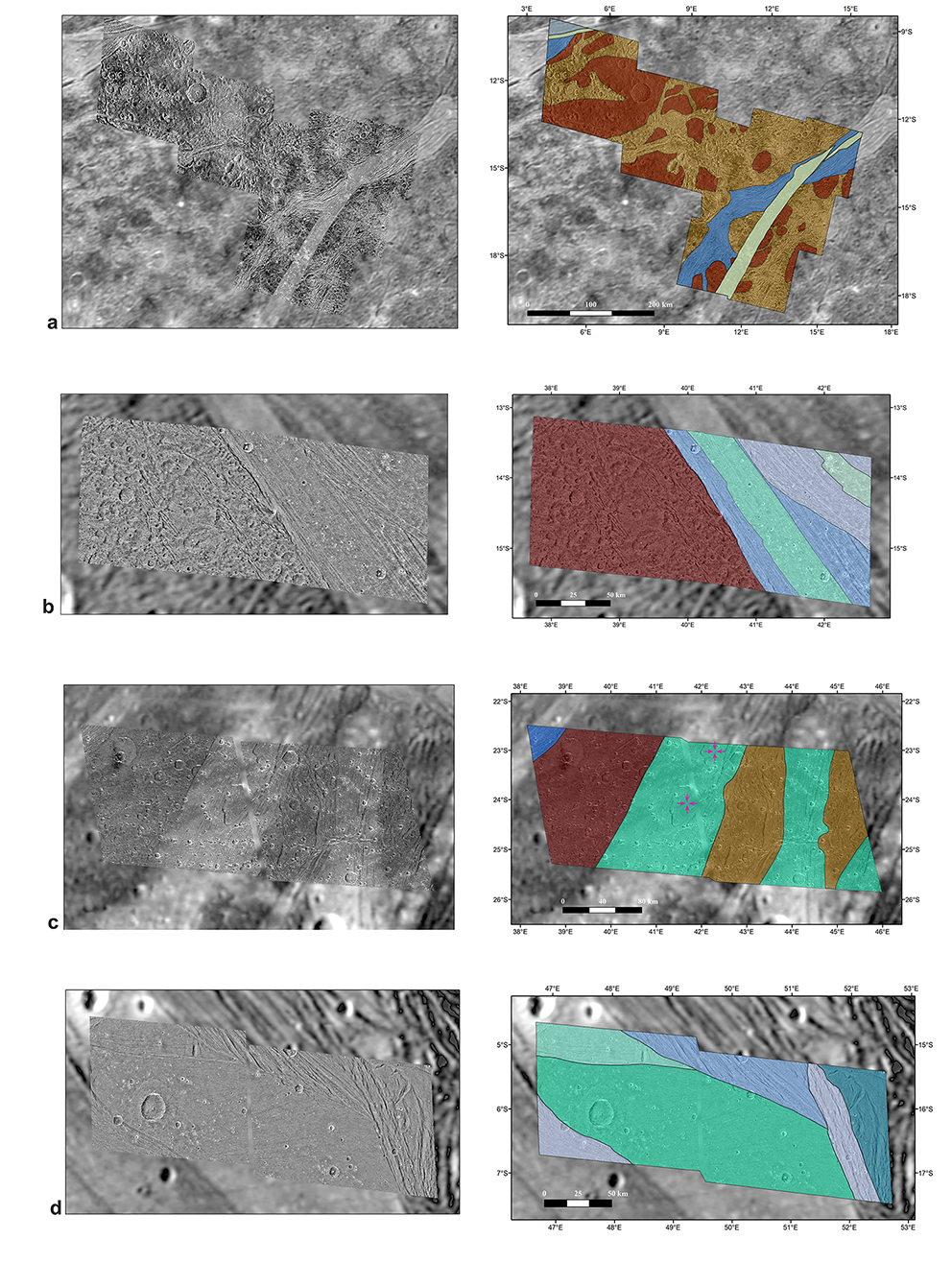
Figure 3: Geologic mapping results for Region B dominated by Arbela Sulcus (28GSARBELA01+02/ G7GSNICHOL01) and Region C by Harpagia Sulcus (b) 28GSBRTDRK02, c) 28GSCALDRA02 and d) 28GSSMOOTH02).
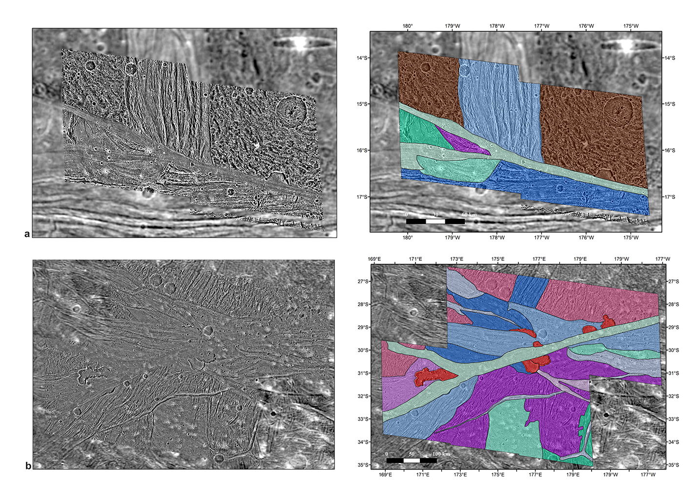
Figure 4: Geologic mapping results for Region D comprises of a) Erech (G8GSERECH01) and b) Mummu and Sippar Sulci (G8GSCALDRA01).
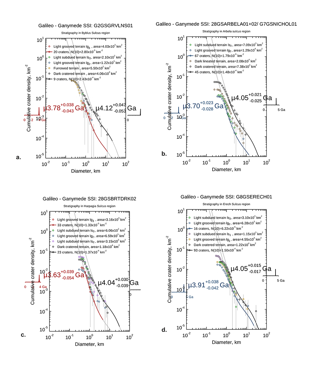
Figure 5: Comparison of relative ages of different terrain units from a) Region A (Byblus Sulcus), b) Region B (Arbela Sulcus), c) Region C (Harpagia Sulcus - 28GSBRTDRK02) and d) Region D (Erech Sulcus) based on crater size frequency distributions.
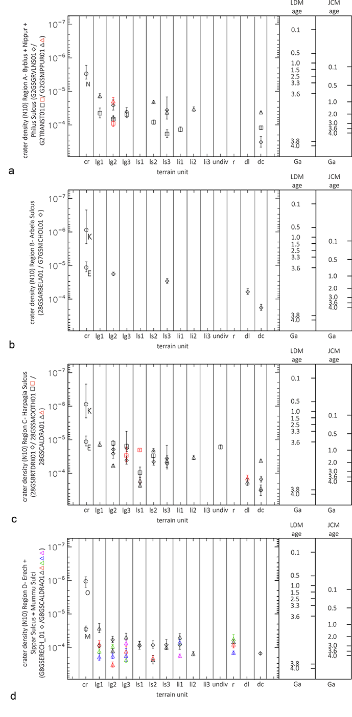
Figure 6: Stratigraphic correlation of Region a) A, b) B, c) C and d) D in which relative ages are determined by plotting the N(10) values with respect to each terrain units and corresponding ages based on LDM [7] and JCM [8]models. Please note that ages of fresh impact craters such as Nergal (N), Kittu (K), Enkidu (E), Melkart (M) and Osiris (O) have been added as additional stratigraphic markers. Since terrain types often appear more than one time in a geologic map the different facies are indicated by different colors.
References:
[1] Grasset, O., et al.: Planetary and Space Science, 78, 1-21, 2013. [2] Stephan, K., et al.: Planetary and space science, 208, 105324, 2021. [3] Pappalardo, R. T., et al.: Jupiter: The Planet, Satellites and Magnetosphere, 363-396, 2004. [4] Collins, G.C., et al.: Global geologic map of Ganymede (p. 3237), US Geological Survey, 2013. [5] Patterson, G. W. et al.: Icarus, 207, 845-867, 2010. [6] Baby, N. R., et al.: LPI Contributions, 2678, abstr. #1350, 2022. [7] Neukum, G., et al.: LPSC XXIX, abstr. #1742, 1998. [8] Zahnle, K., et al.: Icarus 163, 263-289, 2003. [9] Bland, M. T. et al. : Icarus 200, 207- 221, 2009. [10] Bottke et al.: LPSC, #2638, 2022.
How to cite: Baby, N. R., Stephan, K., Wagner, R., Kenkmann, T., Collins, G., Hauber, E., and Jaumann, R.: Stratigraphic relationships of different terrain units on Ganymede and possible implications towards their evolution, Europlanet Science Congress 2022, Granada, Spain, 18–23 Sep 2022, EPSC2022-1016, https://doi.org/10.5194/epsc2022-1016, 2022.
Icy bodies are the most numerous and diverse bodies in the Solar System, but only a few have been visited yet by space probes. Some of these icy bodies, mostly giant planet satellites like Callisto, are called ocean worlds as they likely host most of the liquid water of our Solar System within sub-glacial oceans [Sotin & Tobie 2004]. The presence of liquid water under the icy crusts of these bodies raises questions relative to exobiology. In the coming years and decades, these ocean worlds will be the focus of major planetary science missions, firstly with JUICE (ESA, launch scheduled in April 2023) and Europa Clipper (NASA, launch scheduled in October 2024) which will be targeting the Galilean moons, then with still conceptual missions as we speak such as (i) Uranus Orbiter and Probe and (ii) Enceladus Orbilander. Despite not being the prime target of any of these missions, Callisto will be investigated by JUICE and Europa Clipper through multiple flybys.
One way to get information about Callisto’s sub-glacial ocean is to look at the moon’s surface, which may highlight markers of past or current activity and could lift the veil on its chemical composition. Spectroscopy is a powerful technique for such study, especially in the near-infrared domain where spectral signatures of H2O-ices, silicates, salts are detectable. Consequently, in preparation for future infrared spectroscopic data, and specifically those of the infrared imaging spectrometer MAJIS of the JUICE mission, a ground-based campaign was led with an instrument sharing some similar and also complementary characteristics: SINFONI (SINgle Faint Object Near-infrared Investigation), which was mounted on the UT4 of the VLT at ESO. Here we present the results derived from the analysis and the modeling of four full-disk observations acquired with this instrument.
SINFONI combines an integral field spectrometer operating with different gratings with an adaptive optics module [Eisenhauer et al. 2003]. Our four observations were performed using the H+K grating, ranging from 1.46 µm to 2.41 µm, with a spectral resolution R = 1.500, but each spectrum acquired was automatically resampled in order to get a spectral sampling of 5 x 10⁻⁴ µm. The campaign took place from January 2015 from March 2016, and the observations were acquired near the opposition to optimize the angular resolution with Callisto’s angular diameter close to 1.5 arcsec. As SINFONI’s field of view is 0.8 x 0.8 arcsec2 divided into 64 x 64 pixels, one observation actually corresponds to a mosaic of ten overlapping acquisitions, as described in a paper about Ganymede using the exact same technique [Ligier et al. 2019]. All in all, after removing the high solar incident angle pixels we could not recover after applying photometric corrections (basically all pixels above latitude 60°, north and south), our dataset covers approximately 70% of Callisto’s entire surface with a spectral and spatial sampling (~40 km/pix) which allow to detect and map the spectral absorptions that may exist in this wavelength range of the Callisto’s spectrum. Spatial resolution is in par with that of the partial Callisto mosaic from the NIMS imaging spectrometer of the NASA Galileo probe.
The first results obtained concerns the physical properties of the moon’s surface directly derived from the reduction process and the photometric corrections; one obtains satisfactory results using the qualitative photometric model of Oren-Nayar, which is a generalization of the Lambertian model with the surface roughness (σ) as only additional parameter [Oren & Nayar 1994]. In the case of our study, the best results were obtained with ranging between 17° and 19° whatever the observation. These values are much lower than the values in the 30° – 45° range provided by previous studies [Buratti 1991, Domingue & Verbiscer 1997], however these values were obtained through the modeling of the solar phase curve via the Hapke model [Hapke 1984, Hapke 1986] using a combination of telescopic observations and Voyager data; the major differences between the approaches make the respective results hard to compare (our data are < 10° emergence angle).
Our second result concerns the global shape and spectral signatures in the surface spectra: overall, they are much flatter and more distorted than those of Europa and Ganymede, especially the quite large 2-µm H2O-ice band. To the exception of crystalline ice absorptions at ~1.50 µm, ~1.57 µm, ~1.65 µm and the 2-µm band, Callisto does not show other clear signatures (figure 1). However, very subtle signature(s), like the one at ~2.21 µm (figure 1), might actually be observed and are being investigated to confirm the detection(s). If confirmed it could suggest the presence of hydrated materials like salts or silicates. We will address this point during the meeting.
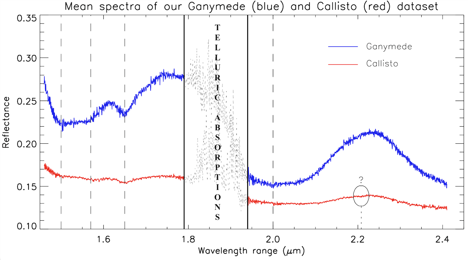
Figure 1: Comparison between Ganymede’s (blue) and Callisto’s (red) mean spectrum of the entire dataset.
And lastly our third main result comes from spectral modeling, where both linear and non-linear unmixing were performed. Unlike previous studies on Ganymede and Europa [Ligier et al. 2019, Ligier et al. 2016], the linear model shows that all of Callisto’s spectra are satisfactorily modeled without needing any hydrated salt and that the only two constituents would be (i) a darkening agent, with abundances always exceeding 80% even for the iciest spectra, and (ii) multiple grain sizes of the crystalline form of H2O-ice, with an average abundance of 7% and exhibiting a strong latitudinal gradient for the smallest grains typical of the influence of the Jovian magnetospheric environment (figure 2). Such a low concentration overall of H2O-ice challenged us about the legitimacy of the linear unmixing approach, so we decided to run the Shkuratov non-linear unmixing model [Shkuratov et al. 1999]. Tests are ongoing but very preliminary results show that the overall concentration of the crystalline ice should be much higher than the 7% coming from the linear model and hence much more representative of what should be the surface composition of an icy satellite. By the time of the meeting, we will be able to present the final results of the study.
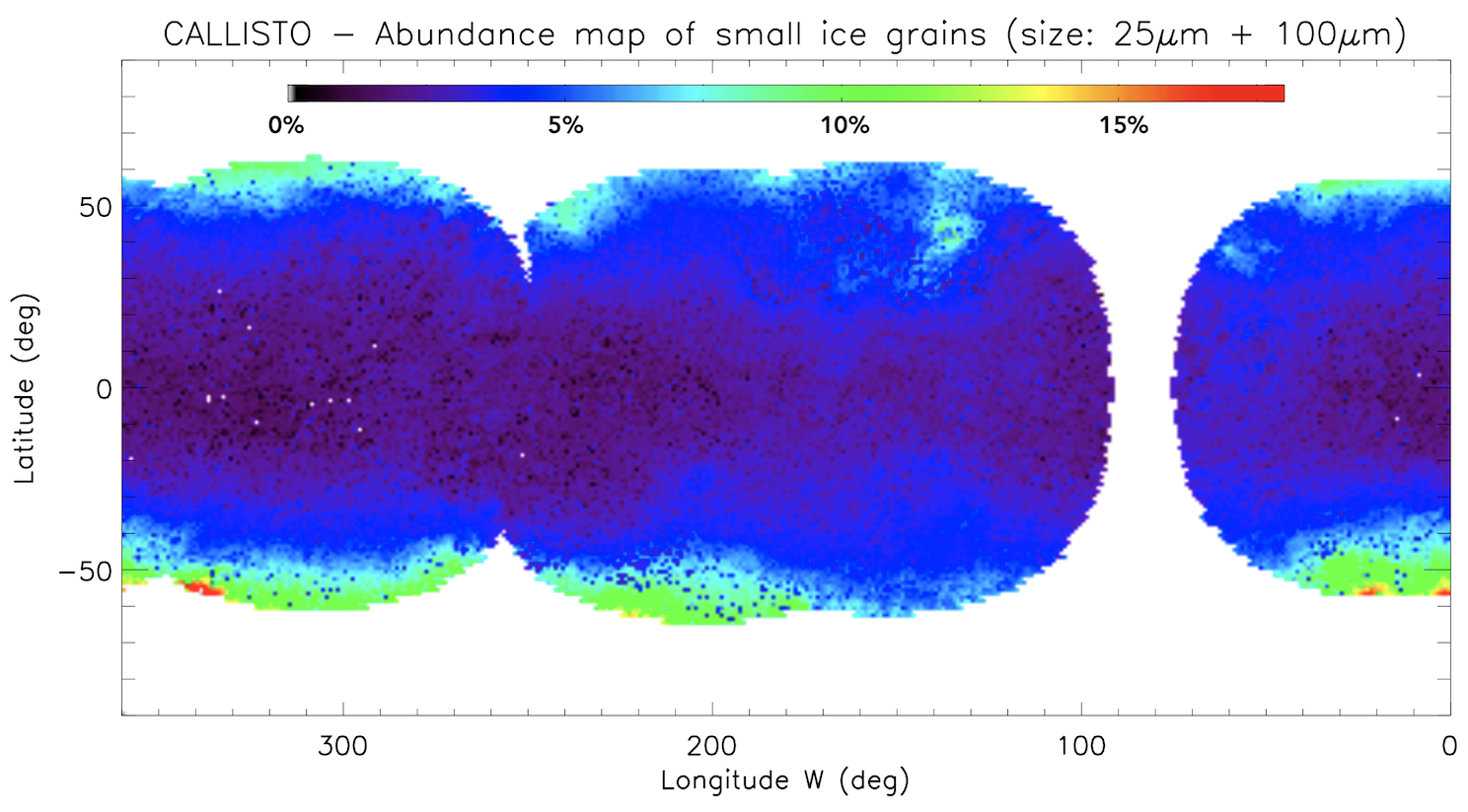
Figure 2: Distribution of the smallest grains of crystalline ice.
How to cite: Ligier, N., Riu, L., Carter, J., Calvin, W. M., Paranicas, C., and Poulet, F.: Pending the next "ocean worlds" missions: Callisto’s surface properties and composition from near-infrared telescopic data, Europlanet Science Congress 2022, Granada, Spain, 18–23 Sep 2022, EPSC2022-1050, https://doi.org/10.5194/epsc2022-1050, 2022.
The María de Maeztu Academy of the Centro de Astrobiología is a two year-long (2019-2020, 2020-2021), tailor-made capacity-building activity implemented within the frame of the “Maria de Maeztu” excellence programme. It aims to strengthen and develop new capacities and stimulate the training of young researchers. The first edition of the transdisciplinary challenges is a training activity of the María de Maeztu Academy intended to develope new skills and generating relevant scientific-technical solutions in the field of Astrobiology. The training program started in September 2021 by forming teams with volunteers from different CAB and INTA departments and different areas of expertise. Throughout 2020-2021, several periodic reviews of the proposals were carried out, passing different milestones and receiving expert comments in each evaluation. Then, the CAB’s MdM Executive Committee decided to financially support the four teams to develop the proposed projects in the 2021/2022 academic year, until the end of the María de Maeztu programme. One of those challenges is “NEXT (iN situ EXploration of planeTary objects): EUROPA” and its objective is to identify the optimal Raman technique for the exploration of the surface of Jupiter´s moon Europa in future missions:
- conducting tests of various Raman techniques (using both commercial and flight models) on representative samples from Europa
- characterizing these samples with the different Raman techniques
- generating a database of pros and cons of each technique, which can minimize risks and optimize expected results

Figure 1 - “NEXT (iN situ EXploration of planeTary objects): EUROPA” logo
In the search for life on other bodies within the Solar System, the top candidates are the icy moons, including Saturn’s moon Enceladus and Europa. These icy moons are target of study as they will help us in the task of assessing possible habitability zones in our neighborhood.
The choice of instruments that can answer these questions and also allow us to understand other factors is key. Raman spectroscopy has the versatility to be used to obtain those answers. It has been widely used in the analysis of terrestrial and planetary samples due to its advantages in rapid and non-destructive analysis of the mineralogy and mineral chemistry of rock and/or soil samples. For planetary explorations it exhibits great potentials for unambiguous phase identification due to its narrow and non-overlapping peak profiles, fast analysis without sample preparations, robust behavior and low mass, etc.
To achieve the stated objectives, a work plan has been established in different stages, subdivided into three phases:
- Samples preparation
- Tests conduction of various Raman techniques on the samples (first is carried out exclusively at the INTA facilities and in the second, the collaborating laboratories will take part)
- Analysis of the test results and database generation of pros and cons of each technique
The samples prepared consist in a saline solution with a molecular organic component. The salt used was MgSO4 that was detected by the Galileo mission [1]. The organic molecule selected was the amino-acid alanine. This amino-acid was discovering in several meteorites as the Murchison meteorite [2]. The sample solutions were prepared with proportions in weight of 5, 10 and 17 % for the salt, and 0.5, 1.0 and 1.5 for the alanine.
The following figures show the multisamples compositions of the nine samples (1 to 9), as a result of the prepared sample vials.

Figure 2 - Multisamples concentrations
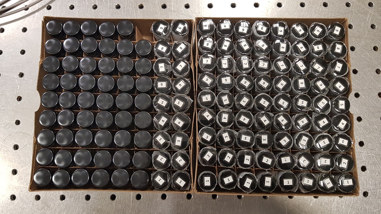
Figure 3 - Prepared multisamples vials
In the second phase, the prepared samples will be analysed in liquid and frozen state with different Raman technologies in four laboratories including the ExoMars RLS [3] Flight Spare model located at INTA. RLS [4] was the first Raman spectrometer qualified for space applications. This phase will be completed in June 2022.
The laboratories where the tests will take place together with the Raman technology to be tested are as follows:
- Centro de Astrobiología (CAB): iHR550 Horiba with an in-situ 532nm laser and portable i-Raman BWTEK with an in-situ 532nm laser
- INTA: ExoMars RLS Flight Spare (in-situ visible green laser). GSE (control and scientific analysis) automated by SW
- University of Valladolid: Raman in-situ Exemplar® Plus LS High Performance Spectrometer with an 785nm (IR) laser and Raman with remote pulsed laser
- Instituto de Micro y Nanotecnología (IMN): LabRaman HR with two possibilities: 532 nm Solid State Diode Laser and 632 nm (HeNe) Solid State Diode Laser
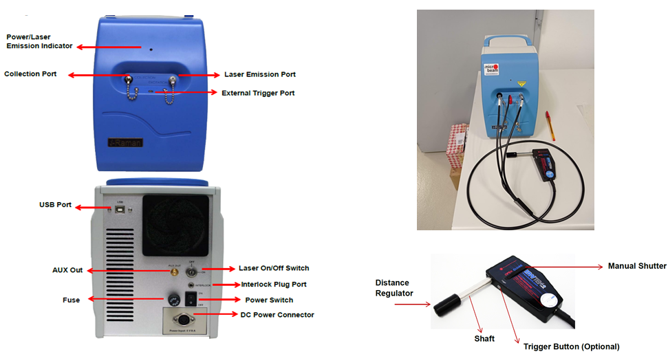
Figure 4 - portable i-Raman BWTEK at CAB facilities
Figure 5 - RLS Flight Spare Model at INTA facilities
With all the information provided by the Raman tests with Raman technology, an analysis of the results will be carried out in July 2022 and conclusions will be issued on the different techniques used to determine and argue which technology (remote or in-situ Raman technology, which excitation laser wavelength: visible / infrared spectrum) would be the most suitable for meet the scientific requirements to address whether life exists or has ever existed in Europa.
[1] Thomas B. McCord, Gary B. Hansen, Jean-Philippe Combe, Paul Hayne, Hydrated minerals on Europa’s surface: An improved look from the Galileo NIMS investigation, Icarus, Volume 209, Issue 2, 2010, Pages 639-650
[2] Engel, M., Nagy, B. Distribution and enantiomeric composition of amino acids in the Murchison meteorite. Nature 296, 837–840 (1982)
[3] Rull, F., et al, The Raman Laser Spectrometer for the ExoMars Rover Mission to Mars, Astrobiology, 2017, vol. 17(6-7), 627-654
[4] Moral, A.G., et al, A Raman Spectrometer for the ExoMars 2020 Rover, European Planetary Science Congress 2017, 17-22 September, 2017, Riga Latvia, id. EPSC2017-1001
How to cite: Zafra, J., Ercilla, O., Sanz, R., Benito, M., Rodriguez Prieto, J. A., Cabrero, J., Moral, A., Prieto Ballesteros, O., and Estrada, A.: “NEXT (iN situ EXploration of planeTary objects): EUROPA”, a challenge to identify the best Raman technique to explore the surface of Jupiter's moon Europa for future missions., Europlanet Science Congress 2022, Granada, Spain, 18–23 Sep 2022, EPSC2022-1088, https://doi.org/10.5194/epsc2022-1088, 2022.
OPS4 | Jupiter and Giant Planet System Science: New Insights From Juno
- Introduction and Summary
Jupiter’s troposphere is divided by eastward (prograding) jets into dynamical domains, which we number sequentially (Figure 1) so the highest-latitude northern domains are N4, N5 and N6 (Figure 2). Here we describe characteristics of these domains with short- and long-term tracking of features that can be identified in JunoCam images. Anticyclonic white ovals (AWOs) and cyclonic folded filamentary regions (FFRs) were tracked in 2021 and earlier years, using amateur images (analysed in the JUPOS project; e.g. Figure 3) and JunoCam maps (from the imager on NASA’s Juno orbiter; e.g. Figure 4) and several Hubble maps (from the OPAL project: ref.1).
The N6 domain is narrow and corresponds to a largely bland zone in JunoCam maps; all features in it are rapidly prograding. The N4 and N5 domains are broad and chaotic with numerous large FFRs and smaller vortices. Their zonal wind profiles (ZWPs) are dominated by the drifts of AWOs and FFRs, but faster retrograde winds exist in the FFRs. Northerly AWOs have rapid prograde drifts, but these often change suddenly, sometimes due to interactions with FFRs or with other AWOs. Most remarkably, in 2021-22 we have one or (very likely) two examples of AWOs moving south to cross prograde jets: one from the N4 domain and one from the N3 domain.
- Zonal drift profiles
Previous spacecraft ZWPs have revealed the overall pattern of the domains: in both N4 and N5, the ZWP is ‘blunt’ with a broad retrograde flow (Figure 1). The Cassini polar movie, and our long-term ground-based analysis [ref.2], suggested that this represents the bulk motion of the rapidly-changing FFRs, and this is confirmed by tracking features in 2021. The mean speeds in L3 are: in N4, +14 deg/30d; in N5, +20 deg/30d. Faster retrograde winds exist in the FFRs. Conversely, AWOs have fast prograding drifts when in the northern part of each domain, but steady retrograding drifts in the southern part, where they often wander in latitude (especially in N4). The largest AWO, in N5, has probably been tracked for at least 3 years and often progrades with the N6 jet. Some smaller AWOs are also long-lived, while others appear and disappear within months.
- Influences on the zonal drifts
In both N4 and N5, AWOs often undergo sudden large changes in their latitude and drift rate (Figure 3) – just as in the N2, S3 & S4 domains. Decelerations are sometimes due to the AWO encountering a FFR, according to examples in the Cassini polar movie and long-term ground-based analysis combined with Hubble maps [ref.2]. Accelerations may sometimes be due to the AWO encountering a smaller white spot. AWOs sometimes pass each other in different latitudes unperturbed, but sometimes their mutual interactions can lead to mergers, or cause one or both to change latitude and speed. In 2021, a pair in N5 rebounded exchang-ing tracks, and other interactions may have propelled a N4 and a N3 AWO southwards to cross the jet.
- AWOs crossing prograde jets
Coherent circulations almost never cross prograde jets on Jupiter, but ground-based data has demonstrated two previous instances where a N4 AWO crossed the N4 jet into the N3 domain, and in 2021-22 there was probably a third such event, captured in JunoCam images. N4-AWO-A swung rapidly southwards after it approached N4-AWO-B (Figures 3 & 4), and was last seen at PJ39, straddling the N4 jet and split into two lobes (Figure 4).
Likewise, a N3-AWO swung southwards and crossed the N3 jet into the NNTZ – the first time that a spot has been seen to cross a prograde jet other than the N4 jet.
- Cloud textures
JunoCam provides unprecedented resolution on the cloud-tops in this region, revealing features such as ‘pop-up clouds’; these are small, very bright white clouds only ten(s) of km across, projecting above the main cloud deck [ref.3], seen in many locations including AWOs, FFRs, and linear white cloud bands outside the main circulations (Figure 5). AWOs have thick white cloud cover with spiral streaking and scattered pop-up clouds. There are also much smaller vortices, both anticyclonic and cyclonic; the latter include well-formed orange-brown spiral cyclones, and ovals with quiescent dark brown cloud-covered interiors. FFRs have a variety of white, grey and orange clouds and hazes that appear to be at different levels. Dense rows of pop-up clouds are commonly seen on the white strips in FFRs, possibly representing the uppermost layer of convection. These white strips are probably thunderstorms, as FFRs in N4 are the most frequent location on the planet for lightning strikes [ref.4].
Acknowledgements: Some of this research was funded by NASA. A portion of this was distributed to the Jet Propulsion Laboratory, California Institute of Technology.
References:
1. Simon AA, Wong MH & Orton GS, NASA & ESA: OPAL project: https://archive.stsci.edu/prepds/opal/. See this website for maps and credits.
2. Rogers J et al., (2017), ‘Jupiter’s high northern latitudes: patterns and dynamics of the N3 to N6 domains.’ https://britastro.org/node/11328
3. Hansen C et al. (2019), ‘JunoCam images of castellanus clouds on Jupiter.’ AGU abstract #P44A-05.
4. Brown S et al.(2018), ‘Prevalent lightning sferics at 600 MHz near Jupiter’s poles.’ Nature 558, 87-90.
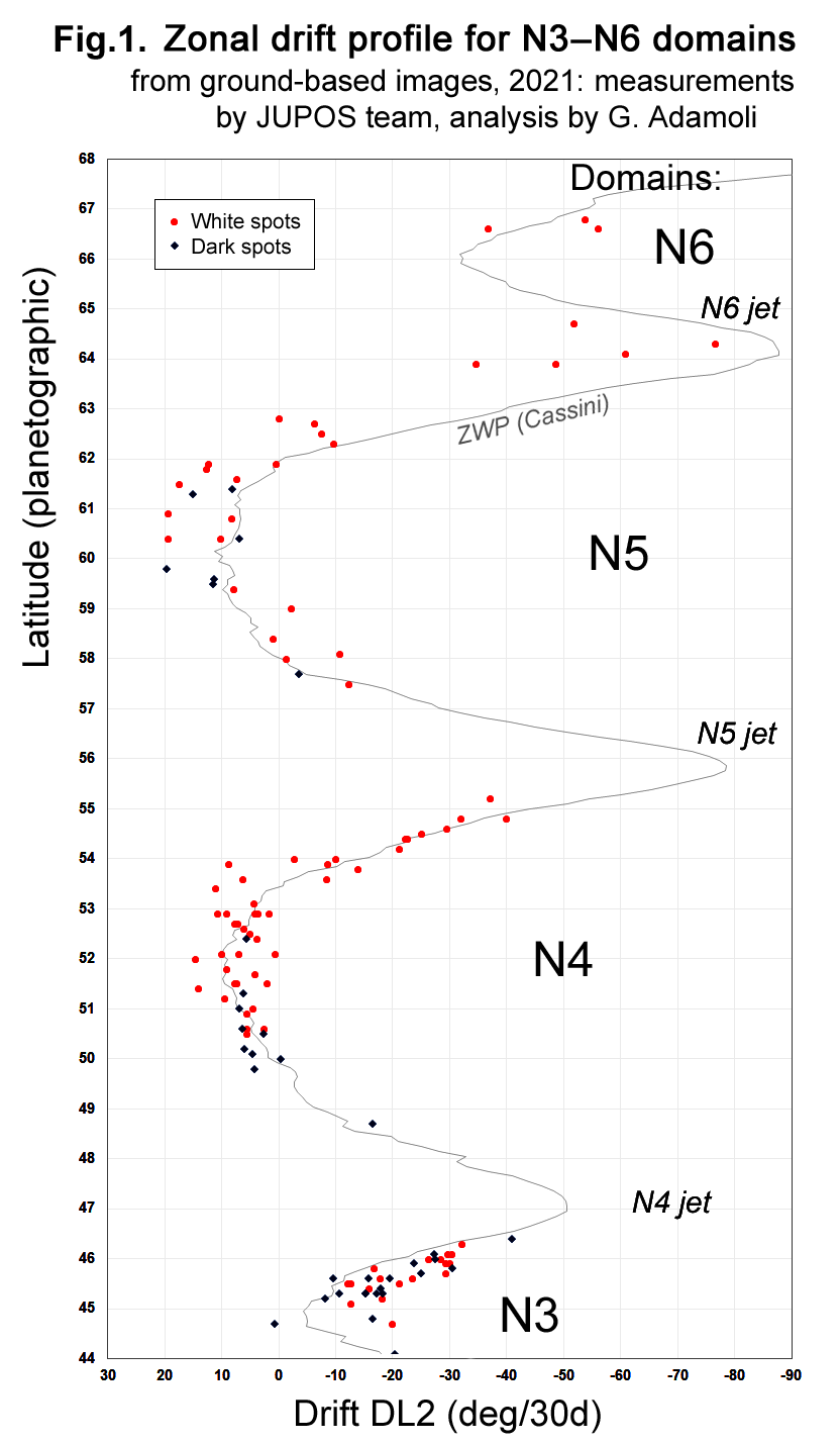


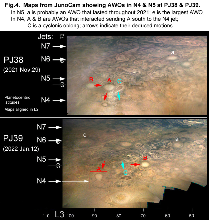
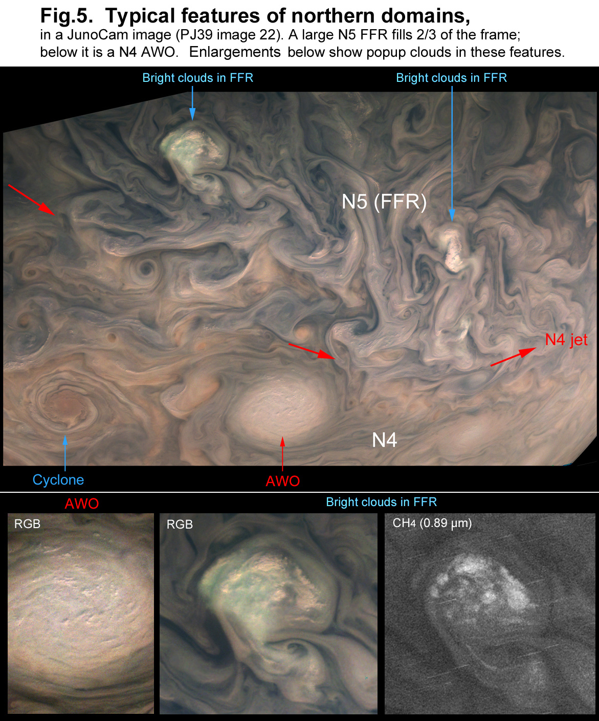
How to cite: Rogers, J., Adamoli, G., Hansen, C., Eichstädt, G., Orton, G., Momary, T., Jacquesson, M., Bullen, R., and Mettig, H.-J.: Jupiter’s high-latitude northern domains: Dynamics from Earth-based and JunoCam imaging, Europlanet Science Congress 2022, Granada, Spain, 18–23 Sep 2022, EPSC2022-16, https://doi.org/10.5194/epsc2022-16, 2022.
The study of Jupiter’s atmosphere, its composition, evolution, distribution, structure, and dynamics around the planet, is of interest to the scientific community. Several missions, space observatories, and ground-based telescopes (even if limited by the telluric bands of water vapor), have studied Jupiter’s atmosphere. Some of them, such as Juno, the Hubble Space Telescope (HST), and the Very Large Telescope (VLT), continue providing information about the vertical structure and distribution of the atmosphere around the planet [1-3]. Although the main chemical composition of Jupiter’s atmosphere has been unraveled, many questions remain open, such as the global abundance of water, or the responsible chemistry for the coloration of the clouds [4]. Besides, a remarkable potential of VIS-NIR spectrometry for characterizing the composition and dynamics of planetary atmospheres has been demonstrated in the last years [5].
The next mission to the Jovian system from the European Space Agency (ESA) is the Jupiter Icy Moons Explorer (JUICE), to be launched in April 2023 with an arrival date on July 2031 [6]. One of the key scientific instruments onboard is the Moons And Jupiter Imaging Spectrometer (MAJIS), which will provide hyperspectral capabilities through two channels: VIS-NIR (0.5μm-2.35μm), and IR (2.25μm-5.54μm) [7]. We would like to perform simulations of different test cases with respect to the viewing geometries of MAJIS and assess its capabilities [8-9] to characterize the vertical structure of the Jovian atmosphere. For this purpose, we upgraded ASIMUT-ALVL, a Radiative Transfer (RT) code developed at BIRA-IASB, that has been extensively used to characterize Mars and Venus atmospheres [10-11].
During the implementation phase of the new Jupiter case in ASIMUT-ALVL, we applied the current knowledge of the physical and chemical characteristics of Jupiter, including the Rayleigh scattering contribution due to dominant atmospheric species, the refractive index of Jupiter’s atmosphere, and the Collision-Induced Absorption (CIA) due to H2-H2 and H2-He molecular systems. The typical temperature profile and atmospheric composition of Jupiter were retrieved from [12], although in our next studies we might use the CH4 abundance from the Volume Mixing Ratio (VMR) profile from [13], which is similar to that from [14]. The required line-lists were implemented from the HITRAN online database with line parameters adequate for an H2 and He dominant atmosphere, following the 2020 version release [15]. The extinction coefficient due to Rayleigh Scattering is obtained based on the calculation of its cross-section from [16], by considering the refractive indexes of H2 and He, obtained from the refractivities measured by [17] and [18], respectively. The atmospheric King correction factor is obtained from an adapted version of the formula of [19], considering the depolarization ratio of H2 as measured by [20]. To model the aerosols and hazes present in the atmosphere, we used the microphysical parameters defined by [21].
We validated the updated performances of ASIMUT-ALVL by individually comparing the main spectroscopic features of Jupiter’s atmosphere in the VIS-NIR range against KOPRA, an RT code originally developed for studying Earth’s atmosphere but later adapted to the atmospheres of Titan, Mars, and Jupiter [22]. We used the same geometry of observation, assuming solar occultations with a tangential altitude between 50km and 360km, a resolution of 0.3cm-1, a Signal-to-Noise Ratio (SNR) of 100, and an orbit around the planet of 5000km high. The mean difference in transmittance obtained between both models is below 3%.
The next step was to validate our RT model against observational spectroscopic data, which was obtained from the Visible and Infrared Mapping Spectrometer (VIMS) observations during the Cassini flyby to Jupiter [23]. This imaging spectrometer consists of two channels: VIS (0.35µm-1.07µm) and IR (0.85µm-5.1µm). In this presentation, we will discuss the results we obtained from the complete validation of our RT model, and the perspectives for the future implementation of the performances and viewing geometries of MAJIS/JUICE.
Acknowledgements
We acknowledge the kind support of Gianrico Filacchione who provided the calibrated data of the VIMS/Cassini observations. This project also acknowledges the funding provided by the Scientific Research Fund (FNRS) through the Aspirant Grant: 34828772 MAJIS detectors and impact on science.
References
[1] Bolton, S.J., et al., Space Science Reviews, 2017. 213(1): p. 5-37.
[2] Nichols, J.D., et al., Geophysical Research Letters, 2017. 44(15): p. 7643-7652.
[3] Antuñano, A., et al., The Astronomical Journal, 2019. 158(3): p. 130 (28).
[4] MAJIS Team, JUICE Definition Study Report, 2014.
[5] Langevin, Y., et al., Lunar and Planetary Science Conference, 2014. No. 1777: p. 2493.
[6] Grasset, O., et al., Planetary and Space Science, Vol. 78, pp. 1-21, 2013.
[7] Piccioni, G. et al., International Workshop on Metrology for AeroSpace, IEEE, 2019. pp. 318-323.
[8] ESA, Consolidated Report on Mission Analysis (CReMA), Tech. Rep. 5.0b23.1. https://www.cosmos.esa.int/web/spice/spice-for-juice
[9] Cisneros-González, M. E. et al., Space Telescopes and Instrumentation in Proc. SPIE 2020, 11443, 114431L.
[10] Vandaele, A.C., et al., Planetary and Space Science, 2015. 119: p. 233-249.
[11] Vandaele, A.C., et al., Optics Express, 2013. 21(18): p. 21148-21161.
[12] Moses, J.I., et al., Journal of Geophysical Research: Planets, 2005. 110(E8).
[13] Sánchez-López, et al., Astronomy & Astrophysics, 2022. Forthcoming article (ArXiv:2203.10086).
[14] Seiff, A., et al., Journal of Geophysical Research: Planets, 1998. 103(E10): 22857-22889.
[15] Gordon, I.E., et al., Journal of Quantitative Spectroscopy and Radiative Transfer, 2022. 277: p. 107949.
[16] Sneep, M., et al., Journal of Quantitative Spectroscopy and Radiative Transfer, 2005. 92(3): p. 293-310.
[17] Peck, E.R. et al., Journal of the Optical Society of America, 1977. 67(11): p. 1550-1554.
[18] Mansfield, C.R., et al., Journal of the Optical Society of America, 1969. 59(2): p. 199-204.
[19] Tomasi, C., et al., Applied optics, 2005. 44(16): p. 3320-3341.
[20] Parthasarathy, S., Indian Journal of Physics, 1951. 25: p. 21-24.
[21] López-Puertas, M., et al., The Astronomical Journal, 2018. 156.4: 169.
[22] Stiller, G.P., et al., Optical Remote Sensing of the Atmosphere and Clouds, SPIE 2000, 3501.
[23] Brown, R.H., et al., Icarus, 2003. 164(2): p. 461-470.
How to cite: Cisneros González, M. E., López-Puertas, M., Erwin, J., Vandaele, A. C., Lauzin, C., Poulet, F., and Robert, S.: Validation of ASIMUT-ALVL against observational data of Jupiter’s atmosphere, Europlanet Science Congress 2022, Granada, Spain, 18–23 Sep 2022, EPSC2022-145, https://doi.org/10.5194/epsc2022-145, 2022.
Jupiter's stratospheric chemistry and dynamics are poorly understood as a function of latitude. The Shoemaker-Levy 9 comet impacts in Jupiter's atmosphere in 1994 have offered us with a unique means to characterize Jupiter's stratospheric chemistry and dynamics. We can indeed use the delivery at 44°S of the long-lived species HCN, CO, H2O, and CS and the subsequent temporal evolution of their spatial distribution as constraints for vertical and meridional mixing, zonal winds and chemistry as a function of latitude.
We mapped HCN and CO in Jupiter's stratosphere with ALMA in March 2017. These observations have already been used in Cavalié et al. (2021) and Benmahi et al. (2021) to derive the stratospheric zonal wind field. In this paper, we use the same observations to retrieve the vertical and meridional distributions of HCN and CO, almost 25 years after the comet impacts. We will present the spatial distributions of both species and discuss the implications on Jupiter's stratospheric chemistry, and vertical and horizontal mixing.
How to cite: Cavalié, T., Rezac, L., Moreno, R., Lellouch, E., Fouchet, T., Benmahi, B., Greathouse, T. K., Sinclair, J. A., Hue, V., Hartogh, P., Dobrijevic, M., Carrasco, N., and Perrin, Z.: ALMA observations of the spatial distribution of CO and HCN in the stratosphere of Jupiter, Europlanet Science Congress 2022, Granada, Spain, 18–23 Sep 2022, EPSC2022-355, https://doi.org/10.5194/epsc2022-355, 2022.
At Jupiter, magnetosphere-ionosphere coupling gives rise to intense auroral emissions and enormous energy deposition in the magnetic polar regions. Here we show ground-based maps of Jupiter's upper atmosphere temperatures obtained via the emissions of the major upper-atmospheric ion, H3+. The maps have a spatial resolution of 2o longitude and latitude from pole to equator and trace the global temperature gradient. We find that temperatures decrease steadily from the auroral polar regions to the equator, indicating that the aurora act as a planet-wide heating source. However, during a period of enhanced activity in the auroral region which models imply was due to a solar wind compression, a high-temperature planetary-scale-sized structure was also observed on top of this gradient. This presentation reports on the particulars of this feature, including how it appears to be propagating away from the main auroral oval (as determined by estimates of the features' velocity at several longitudes) and its subsequent implications for global energy circulation at Jupiter and other planets.
How to cite: O'Donoghue, J., Moore, L., Bhakyapaibul, T., Johnson, R., Melin, H., and Stallard, T.: A planetary-scale heat wave in Jupiter's mid-latitude upper atmosphere, Europlanet Science Congress 2022, Granada, Spain, 18–23 Sep 2022, EPSC2022-373, https://doi.org/10.5194/epsc2022-373, 2022.
Ground- and space-based remote sensing, from Voyager, to Galileo, Cassini and Juno, has revealed the existence of circulation cells in the troposphere of Jupiter. These circulation cells, which may be similar to terrestrial Ferrel cells [1], show properties that vary significantly as a function of depth, showing circulations of opposing directions above and below the expected level of the water condensation cloud near 4-6 bar [2]. Moreover, the location of each vertical branch of the Ferrel-like cells are correlated to the Jupiter's temperature belt/zone contrast, suggesting a dynamical and thermal link between winds, temperatures, aerosols, and composition.
To provide infrared support for Juno spacecraft observations, we have been observing Jupiter with the VISIR mid-infrared instrument on the Very Large Telescope (VLT) since 2016. We analyse images at multiple wavelengths between 5 and 20 µm to study the thermal, chemical and aerosol structure of Jupiter's belts, zones, and polar domains. In particular, an observing run in May 2018 (conciding with Juno's 13 perijove) provided global coverage of Jupiter in thirteen narrow-band filters. These data sense stratospheric temperature (7.9 µm), tropospheric temperature via the collision-induced hydrogen-helium continuum (13, 17.6, 18.6, 19.5 µm), aerosol opacity (8.6 and 8.9 µm), and the distribution of ammonia gas (10.5, 10.7 and 12.3 µm). These wavelengths primarily sound the upper troposphere at p<0.7 bar, above the cloud tops, so are sensitive to the upper cell of the belt/zone Ferrel-like circulations. By stacking the data in all 13 filters, we invert the data using the optimal-estimation retrieval algorithm NEMESIS [3] to derive temperature, aerosol and chemical structure over the whole planet. Meridional gradients of temperature, wind shear (derived from thermal balance equation) and chemical species will be examined to understand the upper-tropospheric circulation cells.
We confirm that the pattern of cool anticyclonic zones and warm cyclonic belts persists throughout the mid-latitudes, up to the boundary of the polar domains. This implies, via thermal wind balance, the decay of the zonal jets as a function of altitude throughout the upper troposphere. Aerosol opacity is often (but not always) highest in the anticyclonic zones, suggesting condensation of saturated vapours, but we caution that aerosol opacity is not a good proxy for atmospheric circulation on any giant planet. The thermal and compositional gradients derived from the VISIR maps are consistent with those from Voyager and Cassini, but opposite to what would be inferred for the Ferrel-like circulations of the deeper cell of [1], which was suggested by [2] to exist only below the water-cloud layer based on Juno microwave observations.
Concerning the Jovian polar regions, the analysis of VISIR imaging shows a large region of mid-infrared cooling poleward ~67˚S, co-located with the reflective aerosols observed in methane-band imaging by JunoCam, suggesting that they play a key role in the radiative cooling at the poles, and that this cooling extends from the upper troposphere into the stratosphere. These VISIR observations also reveal thermal contrasts across polar features, such as numerous cyclonic and anticyclonic vortices, as well as evidence of high-altitude heating by auroral precipitation. Comparison of zonal mean thermal properties and high-resolution visible imaging from Juno allows us to study the variability of atmospheric properties as a function of altitude and jet boundaries, particularly in the cold southern polar vortex. To investigate the radiative processes and influence of auroral precipitation on the southern cold vortex, a radiative-convective model tailored for Jupiter's atmosphere [4], with an updated polar aerosol distribution from Juno mission results, will be used to determine the aerosol distribution needed to reproduce the thermal structure of the cold polar vortex of Jupiter.
[1] Duer, K., Gavriel, N., Galanti, E., Kaspi, Y., Fletcher, L. N., Guillot, T., Bolton, S. J., Levin, S. M., Atreya, S. K., Grassi, D., Ingersoll, A. P., Li, C., Li, L., Lunine, J. I., Orton, G. S., Oyafuso, F. A., Waite, J. H.: Evidence for Multiple Ferrel-Like Cells on Jupiter, Geophysical Research Letters, 2021.
[2] Fletcher, L. N., Oyafuso, F. A., Allison, M., Ingersoll, A., Li, L., Kaspi, Y., Galanti, E., Wong, M. H., Orton, G. S., Duer, K., Zhang, Z., Li, C., Guillot, T., Levin, S. M., Bolton, S: Jupiter's Temperate Belt/Zone Contrasts Revealed at Depth by Juno Microwave Observations, Journal of Geophysical Research: Planets, 2021
[3] Irwin, P. G. J., Teanby, N. A., de Kok, R., Fletcher, L. N., Howett, C. J. A., Tsang, C. C. C., Wilson, C. F., Calcutt, S. B., Nixon, C. A., Parrish, P. D.: The NEMESIS planetary atmosphere radiative transfer and retrieval tool, Journal of Quantitative Spectroscopy & Radiative Transfer, 2008
[4] Guerlet, S., Spiga, A., Delattre, H., Fouchet, T.: Radiative-equilibrium model of Jupiter's atmosphere and application to estimating stratospheric circulations, Icarus, 2020
How to cite: Bardet, D., Donnelly, P., Fletcher, L. N., Antuñano, A., Roman, M. T., Orton, G. S., Guerlet, S., Melin, H., and Harkett, J.: Investigating Thermal Contrasts Between Jupiter's Belts, Zones, and Polar Vortices with VLT/VISIR, Europlanet Science Congress 2022, Granada, Spain, 18–23 Sep 2022, EPSC2022-535, https://doi.org/10.5194/epsc2022-535, 2022.
In 2012, ground-based observations of the dominant molecular ion in gas giant ionospheres, H3+, found that Jupiter’s upper atmosphere was super-heated above its iconic Great Red Spot (GRS). Temperatures there reached 1600 K, hotter even than the auroral region. It was speculated that this GRS “hotspot” was the signature of coupling between Jupiter’s lower and upper atmosphere, perhaps associated with upward propagating acoustic or gravity waves originating from the Solar System’s most powerful storm system. Such an energy transfer could help explain why observed upper-atmospheric gas giant temperatures are all significantly warmer than simulations based solely on solar heating can explain, a discrepancy colloquially referred to as the “giant planet energy crisis”.
Here, based on ground-based observations from 2016-2019, we report on spatial and temporal variations of H3+ temperature surrounding the GRS. We find that, while upper-atmospheric temperatures are still elevated above the GRS, they vary in time and are significantly cooler than in 2012. In addition, there are consistent spatial variations, with H3+ temperature generally highest on the western and northern edges of the GRS. We place these results in context with recent work that implicates Jupiter’s aurorae as primary sources of upper-atmospheric heating, and comment on their implications for Jupiter’s energy crisis.
How to cite: Moore, L., Stallard, T., O'Donoghue, J., Melin, H., Chowdhury, M. N., Johnson, R., Vogt, M., Schmidt, C., and Orton, G.: Ionospheric temperature variability above Jupiter’s Great Red Spot, Europlanet Science Congress 2022, Granada, Spain, 18–23 Sep 2022, EPSC2022-564, https://doi.org/10.5194/epsc2022-564, 2022.
The grand appearance of Jupiter’s banded atmosphere, coloured with many shades from white to red, whose cloud structure currently remains elusive with no clear single cloud model responsible for this varied appearance. With a general pattern of alternating bright cloudy zones and darker belts, as well as unique regions such as the Great Red Spot, finding a way to model all of these differing appearances with a single model has proven difficult. Jupiter’s atmosphere provides continual challenges when attempting to characterise its cloud structure due to its frequently varying appearance. This leads to differences between every observation meaning that models are constantly having to adapt to be explain these changes. Such changes can be seen in Figure 1, both of these spectra have been extracted for the same region of the Equatorial Zone (EZ) but are not identical due to the changes in appearance over the 3 years.
Recent works [1,2,3,4] have all attempted to model Jupiter’s atmosphere using a universal chromophore (cloud colouring compound), combined with a deeper conservatively-scattering cloud and also a stratospheric haze layer. These works have all been able to model the atmosphere successfully but it has currently not been possible to determine between these differing solutions to find the most likely representation of the atmosphere. As all the different sets ups have several ways to vary cloud structure and chromophore properties among other parameters, they have been able to fit the changes in the observations. Therefore keeping each set up viable even as the atmosphere changes. The current inability to conclude on a favoured cloud structure highlights the highly degenerate nature of this problem.
Utilising new observations and techniques to analyse the data highlights the delicacy of these results as the previous set ups have to be altered in order to produce the desired fit to the new observations once the input have varied slightly. An unchanged fit is shown in Figure 1, where the ideal fit of the EZ in 2018 has been used for 2021 data and is unable to model the spectra as well as for the spectra which it was derived from. Furthermore introduction of a limb viewing technique, as used in [2], has been done for this data. Here we attempt to fit multiple viewing angles simultaneously, which also begins to question the robustness of these results, due to an inability of nadir derived set ups to reproduce the multiple observations as successfully.
Therefore in this work we have begun to attempt to reduce the degeneracy of the problem before utilising the Non-linear optimal Estimator for Multi-variatE spectral analySIS (NEMESIS) radiative-transfer retrieval algorithm [5], to fit to our observations. From this we want to find a vertical cloud structure which is more reproducible using different observations and techniques. It is hoped that reducing one of the degenerate parameters before fitting will allow us to constrain the atmospheric structure more decisively. Furthermore combining this with the limb darkening technique will hopefully allow us to rule out some of the solutions to this highly degenerate problem to find more confidence in the proposed models.
In this work we will present the preliminary results taken from the application of these methods to observations to derive a new atmospheric model which can be compared with past work. Additionally we will present the use of new techniques to determine the ability of previous models to adapt to new observations to see if they are still viable.

Figure 1: Spectra of the Equatorial Zone in both 2018 and 2021 and the spectral fit using the model from [1] derived for the 2018 data.
[1] Braude, A. S., Irwin, P. G., Orton, G. S., and Fletcher, L. N. (2020). Colour and tropospheric cloud structure of jupiter from muse/vlt: Retrieving a universal chromophore. Icarus, 338:113589.
[2] Pérez-Hoyos, S., Sánchez-Lavega, A., Sanz-Requena, J., Barrado-Izagirre, N., Carrión-González, O., Anguiano-Arteaga, A., Irwin, P., and Braude, A. (2020). Color and aerosol changes in jupiter after a north temperate belt disturbance. Icarus, 352:114031.
[3] Dahl, E. K., Chanover, N. J., Orton, G. S., Baines, K. H., Sinclair, J. A., Voelz, D. G., Wijerathna, E. A., Strycker, P. D., and Irwin, P. G. J. (2021). Vertical structure and color of jovian latitudinal cloud bands during the juno era. The Planetary Science Journal, 2(1):16.
[4] Baines, K., Sromovsky, L., Carlson, R., Momary, T., and Fry, P. (2019). The visual spectrum of jupiter’s great red spot accurately modeled with aerosols produced by photolyzed ammonia reacting with acetylene. Icarus, 330:217–229.
[5] Irwin, P. G. J., Teanby, N. A., de Kok, R., Fletcher, L. N., Howett, C. J. A., Tsang, C. C. C., Wilson, C. F., Calcutt, S. B., Nixon, C. A., and Parrish, P. D. (2008). The NEMESIS planetary atmosphere radiative transfer and retrieval tool. , 109:1136–1150
How to cite: Alexander, C. and Irwin, P.: Comparing atmospheric models of Jupiter, can we reduce the degeneracy of this problem?, Europlanet Science Congress 2022, Granada, Spain, 18–23 Sep 2022, EPSC2022-632, https://doi.org/10.5194/epsc2022-632, 2022.
The Juno Microwave Radiometer (MWR) has extended our knowledge of the structure and composition of Jupiter's atmosphere down to several hundred bars, revealing meridional variability at great depths (e.g. Li et al. 2017, Fletcher et al. 2021). It has revealed that some cyclonic and anticyclonic vortices may have roots at depths of hundreds of bars of pressure (Bolton et al. 2022), but 5-µm hot spots and associated plumes are restricted to shallow depths above the water cloud (Fletcher et al. 2021). We report ongoing work on evolution of axisymmetric bands, concentrating on two regions where large-scale changes have been observed in the visible and infrared.
One of these is the Equatorial Zone (EZ), for which Figure 1 illustrates a dramatic color change. The color change in the central component (EZc, ~3°S – 1°N, planetocentric latitude) is more prominent than the northern component (EZn, ~2° - 6°N). This change began in 2018, and by 2019 was as prominent as shown in 2021. In near-infrared bands of strong gaseous absorption, the EZc reflectivity increased dramatically (Fig. 2), but only temporarily for the EZn.
Another region is the northern component of the North Equatorial Belt (NEBn, ~12°N to 15°N), whose change from a visibly dark to a bright region is also illustrated in Figure 1, with the southern component (NEBs, ~7°N to 11°N) remaining its typical dark color. Figure 3 shows that this color is associated with a remarkable drop of its 5-µm brightness which dropped down to the faint emissions of the nearby cloudy and visually bright zones. This implies a major increase in the opacity of 0.7-5 bar clouds that are similar but more extreme than the quasi-periodic northward expansions of the NEB (Fletcher et al. 2017). This transformation took place in early 2021 when Jupiter was in solar conjunction.
The very preliminary results of our initial examination of MWR observations (Fig. 4) plot antenna temperatures derived using averages over all longitudes sensed in which the center of the field of view lay within specified latitude ranges. Observations were selected only if 99% or more of the field of view included the planet and the emission angle was limited to 65° or less, after which they were converted to a nadir-equivalent emission using limb-darkening models that were fit to every latitude and each channel. All observations were made at close approaches of the spacecraft to Jupiter, known as ‘perijoves’ or PJs. Many perijoves between 2019 and 2022 did not contain any measurements of these regions meeting those selection criteria, due to unfavorable spacecraft pointing. Exceptions included special spacecraft orientations.
The EZc appears invariable in time, but the EZn underwent a ~7K drop in Channel-3 antenna temperatures - sensitive to conditions near ~9 bars - starting in early 2017, reaching a minimum in late 2017, then returning to its original values by early 2019. Similar variability is evident in Channel 4, sensitive to the ~3-bar level, and a smaller one in Channel 5, which is sensitive to the ~1.5-bar level. No change is detectable in Channel 6, sensitive to the ~0.7-bar level. The 2017 temperature drop has no obvious counterpart in reflected sunlight, although its “recovery” occurs during the reflectivity changes in 2019 (Figs. 1-2). To link the two, one must devise a causal relationship between a short-lived variation of absorber, likely gaseous ammonia, at 1.5-9 bars at 2016-2019 between 2°N and 6°N, and conditions at higher altitudes over a wider latitude range.
If the NEBn variability between 2020 and 2021 (Figs. 1, 3) implies an increase of ammonia absorption, we would expect a decrease in antenna temperatures between our last trustworthy observation in 2019 April and observations in late 2021. This is indeed the case at 0.7 bars, represented by the 6-7K drop in Channel-6 antenna temperatures for the NEBn. This is also present in Channel 5 as a ~5K drop, but it is not detectable above the noise in the deeper-sounding channels, so this is not substantially present at pressures higher than ~1.5 bars. A ~5K drop in antenna temperatures in late 2016 is followed by a slower rise to its previous range by the end of 2017 in both Channels 5 and 6. Other channels do not show this variability, so this is another “shallow” phenomenon with no obvious connection to changes in cloud reflectivity.
We will continue to examine variability in cloud reflectivity associated with these changes, observe with increasingly favorable geometries for the next few perijoves, and examine other latitudes for variability.
References:
Bolton, et al. 2021. Science 374, 968-972.
Fletcher, et al. 2017. Geophys. Res. Lett. 44, 7140-7148
Fletcher, et al. 2020. J. Geophys. Res. 125, E06399.
Fletcher, et al. 2021. J. Geophys. Res. 126, E06858.
Li, et al. 2017. G. Res. Lett. 44, 5317-5325.
Simon, et al. 2015. Ap. J. 812, 55.

Figure 1. Color-composite cylindrical maps of Jupiter from the Hubble Space Telescope OPAL program (Simon et al. 2015). Note the darkening of the EZ central and northern components, which began in 2018. Note also that in 2021 the northern part of the North Equatorial Belt has become lighter in color compared with 2017, a process that took place in early 2021.

Figure 2. Reflectivity of the central and northern components of the Equatorial Zone vs time at 2.166 µm, a wavelength sensitive to reflected sunlight from ~80-mbar aerosols. This plot implies that the EZn contained a denser population of aerosols near this level, most likely from more vigorous lofting.

Figure 3. Images of Jupiter at 5.1 µm: these and data in Fig. 2 were taken using NASA’s Infrared Telescope Facility (IRTF) SpeX guide camera. Note the drop in radiance of the northern section of the North Equatorial Belt from 2020 to 2021.

Figure 4. Preliminary results on radiances measured by Juno’s Microwave Radiometer (MWR). Channels 3 and 6 sense radiances at 2.6 and 22 GHz, respectively. For clarity, other channels are not shown. Error bars represent the standard deviation of antenna temperatures included in the latitude bin.
How to cite: Orton, G., Fletcher, L., Oyafuso, F., Li, C., Zhang, Z., Brueshaber, S., Wong, M. H., Momary, T., Levin, S., Bolton, S., Baines, K., Dahl, E., and Sinclair, J.: Exploring the Depth of Planetary-Scale Changes in Jupiter from Juno Microwave Radiometer Observations, Europlanet Science Congress 2022, Granada, Spain, 18–23 Sep 2022, EPSC2022-761, https://doi.org/10.5194/epsc2022-761, 2022.
Since 2016 the Juno spacecraft has been in orbit around Jupiter, gathering unprecedented data from its highly inclined 53-day orbit. The Jupiter Infrared Auroral Mapper (JIRAM) is an imager and spectrograph with spectral coverage between 2 and 5 µm. This region is dominated by reflected sunlight by aerosols and hazes, with distinct absorptions by ammonia, phosphine, germane and other minor species in Jupiter's troposphere, as well as ionospheric H3+ at high altitude. Here, we outline the process undertaken to model the full spectral coverage of JIRAM with NEMESIS, our radiative transfer and retrieval code (Irwin et al., 2008). This includes altering the NH3 aerosol and haze properties, updating the molecular line-list, and testing the sensitivity to the abundance of the molecular species that are within the 2-5 µm range offered by JIRAM.
This study builds on previous models for JIRAM spectra in thermal emission (Grassi et al., 2020) and reflected sunlight (Grassi et al., 2021), by attempting to fit the entire 2-5 µm range simultaneously with a single consistent aerosol model. The model includes two aerosol layers, a NH4SH type layer at 1.3 bars, and a NH3 type layer at 0.7 bars, as well as a tholin type haze layer that extends from the troposphere to the stratosphere. We demonstrate that JIRAM observations of both reflected sunlight and thermal emission cannot be reproduced simultaneously using standard refractive indices available in the literature. We build a simple model of the refractive indices for the three aerosol layers, adapting the technique of Sromovsky et al. (2010), and demonstrating the improvement in the fits at each step. As a proof of concept we present the analysis of meridionally averaged zonal profiles, investigating how aerosols, ammonia, and phosphine vary with latitude during the early perijoves of the mission.
How to cite: Melin, H., Fletcher, L., Irwin, P., Grassi, D., and Mura, A.: Modelling the full 2-5 µm Juno JIRAM spectral range with NEMESIS: Zonal Profiles of Jupiter’s Aerosols, Condensables, and Disequilibrium Species, Europlanet Science Congress 2022, Granada, Spain, 18–23 Sep 2022, EPSC2022-817, https://doi.org/10.5194/epsc2022-817, 2022.
The shape of gaseous planets, defined as an equipotential surface for a specific pressure, can be calculated given measurements of the zonal gravity harmonics, and the wind profile and polar radius at a given level. For both Jupiter and Saturn, the gravity harmonics have been measured to high accuracy by the Juno and Cassini missions, respectively. Measurements for the zonal winds are also available via cloud tracking, buth a significant uncertainty is associated with them, stemming from the clouds altitudes, as well as time variations in the strength and location of the winds. With that, the wind profiles can be also constrained by the gravity measurements. Further constraint on the calculated shape of the two gas giants can be obtained from occultation measurements, which give radial dependent profiles of pressure for specific spatial location.
Here we propose a new method for calculating the shape of the gas giants, based on an optimization of the wind latitudinal profile, decay structure, and the polar radius, given both gravity and occultation measurements. We use thermal wind balance to relate the wind to the gravity measurements, and a shape model to relate the wind and polar radius to the occultation measurements. We perform the analysis for both the 0.1 and 1 bar pressure levels. We examine the ability to explain both types of measurements in each planet, and discuss the implication for the possible wind profiles and how they might change with pressure. We also discuss the solutions for the polar radius with respect to the currently used mean values.
Only a few occultation measurements are currently available in each planet, but in the coming years the Juno mission is expected to perform dozens of occultations for Jupiter, covering a wide spatial range, and there are several Cassini occultations performed for Saturn that are still waiting for analysis. Using the method proposed here, we expect the new measurements to help resolve the shape of the gas giants to better accuracy, and to allow better understanding of the wind structures and their depth dependence.
How to cite: Galanti, E., Smirnova, M., Kaspi, Y., and Guillot, T.: The shape of Jupiter and Saturn based on winds, occultations and gravity measurements, Europlanet Science Congress 2022, Granada, Spain, 18–23 Sep 2022, EPSC2022-843, https://doi.org/10.5194/epsc2022-843, 2022.
A key feature among the Galilean satellites is their monotonic decrease in density, indicating an ice fraction that is zero in the innermost moon Io, and about half in the outer moons Ganymede and Callisto. So far, there is no formation scenario that explains this gradient while considering the moons grew in a water-depleted circumplanetary disk. Here, we investigate the possibility that the jovian circumplanetary disk was fueled with ice-free chondritic minerals, including phyllosilicates. To do so, we use a standard one-dimensional gas-starved accretion disk model derived from the literature [1, 2] coupled with gas and solids transport modules [3, 4] to investigate the evolution of vapors released by the dehydration of phyllosilicates. We show that the dehydration of such particles and the outward diffusion of the released water vapor allows condensation of significant amounts of ice in the formation region of Ganymede and Callisto in the Jovian circumplanetary disk. This mechanism naturally explains the presence of ice-rich moons around a water-depleted Jupiter.
[1] Canup, R.M., Ward, W.R. 2002. Formation of the Galilean Satellites: Conditions of Accretion. The Astronomical Journal 124, 3404–3423. doi:10.1086/344684
[2] Sasaki, T., Stewart, G.R., Ida, S. 2010. Origin of the Different Architectures of the Jovian and Saturnian Satellite Systems. The Astrophysical Journal 714, 1052–1064. doi:10.1088/0004-637X/714/2/1052
[3] Birnstiel, T., Klahr, H., Ercolano, B. 2012. A simple model for the evolution of the dust population in protoplanetary disks. Astronomy and Astrophysics 539. doi:10.1051/0004-6361/201118136
[4] Anderson, S.E., Mousis, O., Ronnet, T. 2021. Formation Conditions of Titan's and Enceladus's Building Blocks in Saturn's Circumplanetary Disk. The Planetary Science Journal 2. doi:10.3847/PSJ/abe0ba
How to cite: Mousis, O., Schneeberger, A., Lunine, J., Glein, C., Bouquet, A., Vance, S., and Vinogradoff, V.: The role of phyllosilicates in shaping the Galilean moons' density gradient, Europlanet Science Congress 2022, Granada, Spain, 18–23 Sep 2022, EPSC2022-855, https://doi.org/10.5194/epsc2022-855, 2022.
Helium ions, He+, react only slowly with molecular hydrogen. A consequence of this is that He+ ions produced by, for example, photoionization of He in H2-dominated ionospheres, such as those of Jupiter and Saturn, can have principal loss mechanisms other than through reactions with molecular hydrogen even if the other reactants prevail in rather small volume mixing ratios. The Ion and Neutral Mass Spectrometer (INMS) onboard the Cassini mission operated in open-source ion mode during a few of the passages through Saturn’s upper atmosphere throughout the proximal orbits in 2017. Due to the high spacecraft velocity, exceeding 30 km/s, the retrieval of ion number densities was limited to light ion species with masses (for singly charged species) of < 8 Da. The retrieval of number densities of volatiles like H2O, CH4, NH3, N2 and CO were in part complicated by adsorption effects.
We seek to make an independent estimate of the mixing ratios of volatiles other than H2 and He by making use of a simple model focusing on the production and loss balance of helium ions. We first consider two models to estimate the local production rate of He+ from the measured density profiles of He and H2 and show that these give estimates in reasonable agreement with each other. Then we show that the calculated concentration of He+ exceeds the observed values by up to two orders of magnitude if we only account for the loss of He+ ions through reactions with molecular hydrogen. We take this as a strong indicator that the principal loss mechanism of He+ in Saturn’s ionosphere is through reactions with other species than H2. We proceed with a brief survey of chemical reaction databases highlighting that it seems reasonable to consider an effective rate constant of k1 ≈ (1.0 ± 0.5)*10-9 cm3 s-1 for reactions involving the neutralization of He+ in reactions with H2O, CH4, NH3, N2 and CO. This allows us to estimate the mixing ratio of these molecules across an altitude profile. Our results are compatible with the average values reported by Miller et al. (2020) and show indications of enhanced mixing ratios towards lower altitudes and/or near equatorial latitudes.
How to cite: Dreyer, J. and Vigren, E.: Deriving mixing ratios of heavier neutral species in Saturn's ionosphere from light ion measurements, Europlanet Science Congress 2022, Granada, Spain, 18–23 Sep 2022, EPSC2022-1053, https://doi.org/10.5194/epsc2022-1053, 2022.
Introduction
During almost all of Juno's past perijove flybys, JunoCam took images that allowed us to derive cloud velocity field data from cloud feature displacements.
During more recent Jupiter flybys, JunoCam observed distinct cloud top features with very different emission angles within less than ten minutes. These images also show relative cloud feature displacements. These newly observed displacements fields, however, appear to be parallel to vector fields that would be expected from parallaxes induced by long-baseline observations of the cloud top topography rather than primarily from cloud motion.
Based on this assumption, we show stereo images to make these observations intuitive. For this purpose, we project a pair of JunoCam images to the same trajectory position.
The pair of trajectory positions the JunoCam images have actually been taken from can be used to derive a quantitative displacement field in terms of pixels per km altitude offset. Stereo correspondence ís simplified to a one-dimensional search. Observed relative displacements can then be divided by the previously derived scaling in order to retrieve a digital elevation map of relative heights of the cloud tops.
Digital elevation maps can further be rendered in 3D.
Example image pair
This cross-eyed stereo pair is derived from JunoCam images JNCE_2022099_41C00024_V01 and JNCE_2022099_41C00026_V01. The time span between the two images is less than four minutes. For observers trained to cross-eyed vision, the three-dimensional effect of the distinct cloud-top features is well-visible. The image pair can also be transformed into a blink gif or into an anaglyph.

How to cite: Eichstädt, G., Orton, G., and Hansen-Koharcheck, C.: Long-Baseline Observations with JunoCam, Europlanet Science Congress 2022, Granada, Spain, 18–23 Sep 2022, EPSC2022-1124, https://doi.org/10.5194/epsc2022-1124, 2022.
How to cite: Agiwal, O., Moore, L., Martinis, C., Mueller-Wodarg, I., and Huba, J.: First Steps Towards a New Saturn Ionosphere Model Including Ring-Planet Coupling and Electrodynamics, Europlanet Science Congress 2022, Granada, Spain, 18–23 Sep 2022, EPSC2022-1215, https://doi.org/10.5194/epsc2022-1215, 2022.
OPS5 | Outer Planet Moons: Environments and Interactions
We use a three-dimensional hybrid model of plasma (kinetic ions and charge neutralizing electron fluid) to study the dynamics of the thermal O+ and H+ ions at Ganymede's magnetopause when Ganymede is inside and outside of the jovian plasma sheet. Our kinetic simulations show that ion velocity distributions at the vicinity of the upstream magnetopause of Ganymede are highly non-Maxwellian where the dominant component of the velocity distribution is parallel to the background magnetic field (i.e., Tll>T⊥). At the magnetopause, however, ions are substantially heated and the dominant component of the velocity distribution is perpendicular to the background magnetic field (i.e., Tll<T⊥). We also investigate the energization of the ions interacting with the magnetopause and we find that the energy of those particles on average increases by a factor of 8 and 30 for the O+ and H+ ions, respectively. The energy of these ions is mostly within 1-100 keV for both species after interaction with the magnetopause, but a few percentage reach to 0.1-1 MeV. Our simulations show that a small fraction (<25%) of the co-rotating Jovian plasma reach the magnetopause, but among those more than 50% cross the high power density regions at the magnetopause and gain energy. Finally, we compare our simulation results with Galileo observations of Ganymede's magnetopause crossings (i.e., G8 and G28 flybys). There is an excellent agreement between our simulations and observations, particularly our simulations fully capture the size of the magnetosphere and reproduce the sharp magnetic transients at the magnetopause crossings.
How to cite: Fatemi, S., Poppe, A. R., Vorburger, A., Lindkvist, J., and Hamrin, M.: Hybrid simulations of jovian plasma interaction with Ganymede's magnetopause, Europlanet Science Congress 2022, Granada, Spain, 18–23 Sep 2022, EPSC2022-27, https://doi.org/10.5194/epsc2022-27, 2022.
1. Introduction
In preparation of the JUICE mission with the primary target Ganymede [1] we generated a new controlled version of the global Ganymede image mosaic from Voyager 1 and 2 and Galileo images [2] based on a new 3D control point network from Zubarev et al., 2016 [3]. In 2021, the Juno mission acquired new Ganymede images with its onboard wide-angle camera JunoCam [4]. We used the best available images from Perijove 34 to integrate them into the global Ganymede mosaic.
2. Image data
On June 7th, 2021, near the end of Juno’s prime mission, the spacecraft flew by Ganymede to obtain four close-ups of the leading side of the moon from an altitude of about 1046 km. The derived image data has been integrated into the control point network of Ganymede to find a global solution for all three datasets. The new control point network consists of 4968 points.
3. Mosaicking
After aligning the Juno images photogrammetrically to fit onto the global Ganymede mosaic from Voyager and Galileo images brightness and contrast corrections have been applied to the Juno images manually to create a consistent look within the global mosaic. The small crater Anat is defining the longitude system at 232° East and the radius is set to 2631.2 km. The updated version of the global Ganymede mosaic will become available at https://janus.dlr.de/ and will be archived at PSA’s GSF.
4. Outlook
With this work we hope to support the JUICE team during pre-arrival investigations and the observation planning of Ganymede.
References
[1] Grasset et al., 2013, Planetary and Space Science, 78, 1-21, DOI: 10.1016/S0032063312003777. [2] Kersten et al., 2021, Planetary and Space Science 206, DOI: 10.1016/j.pss.2021.105310. [3] Zubarev et al., 2016, Solar System Research, 50, 5, 352-360, DOI: 10.1134/S0038094616050087. [4] Hansen et al., 2017, Space Science Reviews, 213, pages 475-506.
How to cite: Kersten, E., Zubarev, A. E., Nadezhdina, I. E., Roatsch, T., Matz, K.-D., and Szczech, C. C.: Updated Ganymede Mosaic from Juno Perijove 34 Images, Europlanet Science Congress 2022, Granada, Spain, 18–23 Sep 2022, EPSC2022-450, https://doi.org/10.5194/epsc2022-450, 2022.
The Cassini mission explored Saturn’s system from 2004 to 2017. On its board, a RADAR operating at a wavelength of 2.2 cm (13.78 GHz), had been initially designed for the exploration of the surface of Titan but also regularly turned its antenna towards the main airless icy satellites of Saturn (Elachi et al., 2004). In addition to its active mode, the Cassini RADAR included a passive (or radiometry) mode designed to record the thermal emission from the targeted surfaces at 2.2-cm. The scientific objectives of Cassini RADAR icy satellite observations were to provide constraints on the thermal, physical and compositional properties of the first few meters below the surface of the investigated objects. Doing so, it brings insights into the degree of purity and maturity of their water-ice regolith which are both indicative of their geological activity and interaction with their environment.
The RADAR dataset acquired on icy moons has already proved to be very fruitful bringing light to notable differences among Saturn’s mid-sized satellites (Ostro et al., 2006; 2010; Le Gall et al., 2019). However, it has not been fully analyzed yet. Following the final analysis of Cassini RADAR active observations of Saturn’s icy moons described in Le Gall et al. (2019) and expanding and improving upon the work of Ostro et al. (2006; 2010), we here present the analysis of all Cassini distant passive RADAR observations of these objects. This represents a total of 63 observations collected during 4 flybys of Mimas, 10 of Enceladus, 3 of Tethys, 6 of Dione, 9 of Rhea, 3 of Iapetus, 1 of Phoebe.
Most of Cassini RADAR icy satellite observations were distant i.e., occurred at ranges where the antenna beamwidth is comparable to or greater than the apparent angular extent of the target’s disk and were thus primarily designed to provide disk-integrated quantities: hemispheric-averaged radar albedos in the RADAR active mode and disk-integrated brightness temperatures in the passive mode. We here present the reduction of all available Cassini passive radiometry data with the goal of providing a range of possible values for the disk-averaged 2.2-cm emissivity of Saturn’s main airless satellites (separating their leading and trailing sides if relevant). These latter are obtained as a function of their possible thermal and electrical properties using a combined thermal and radiative transfer model (Le Gall et al., 2012; Bonnefoy et al., 2020). As an example, Fig. 1 displays the emissivity values obtained for Mimas from 4 distant radiometry observations. These values are shown as a function the assumed thermal inertia and ratio of electrical and thermal skin depths of Mimas’s near-surface. For all sets of parameters they are very low, as low as 0.5. For comparison, the disk 2.2-cm emissivity of Iapetus (Le Gall et al., 2014), Phoebe and Titan (see Sultana et al., this conference) is close to 0.9. Mimas low emissivity is indicative of subsurface mostly made of pure water ice and where volume scattering is very efficient maybe due to a highly fractured structure. We find that Enceladus and Tethys also exhibit low emissive surfaces and that, as a general rule, moon-to-moon and hemispheric emissivity variations seems to reflect variations in the moon interaction with Saturn’s dust rings, namely the E-ring for Enceladus and its neighbours and Phoebe’s ring further away from Saturn (Iapetus and Phoebe).
The derived emissivities will be analysed in light of the (active) radar albedos measured on the same hemispheres. Both active and passive microwave observations will be compared to several combined emissivity-backscatter models thus providing further clues on the physical properties of the icy moons. Their implications in terms of surface geology and evolution will be discussed.
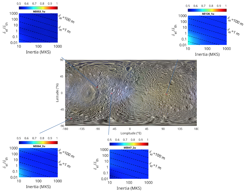
Fig. 1: 2.2-cm emissivity of Mimas’s surface derived from Cassini distant radiometry observations and a combined thermal and radiative transfer model as a function of Mimas subsurface thermal and electrical properties (namely its thermal inertia and the ratio of its electrical and thermal skin depths). The sub-spacecraft point of each distant observation is indicated on an ISS map of the satellite.
How to cite: Le Gall, A., Sultana, R., Bonnefoy, L., Leyrat, C., and Janssen, M. A.: Microwaving Saturn's airless icy moons Mimas, Enceladus, Tethys, Dione, Rhea, Iapetus and Phoebe, Europlanet Science Congress 2022, Granada, Spain, 18–23 Sep 2022, EPSC2022-607, https://doi.org/10.5194/epsc2022-607, 2022.
Ganymede’s water exosphere has been observed spectroscopically on several occasions since the first detection of atomic hydrogen in Ganymede’s exosphere in 1997 [1]. From these observations a consistent picture of Ganymede’s exosphere has emerged: Ganymede’s day-side exosphere is dominated by sublimated water with inferred column densities of up to several 1e15 cm-2, while elsewhere the exosphere is dominated by sputtered molecular oxygen (inferred column densities of several 1e14 cm-2) at low altitudes and by atomic oxygen (inferred column densities of several 1e13 cm-2) at higher altitudes [2-9]. In addition, atomic hydrogen has been observed with inferred column densities of a few 1e12 cm-2 [1, 4, 10]. Whereas many modeling approaches have been able to reproduce the inferred H2O and O2 densities, they have struggled to re-create the high inferred atomic oxygen and hydrogen column densities [11-13].
In this work, we present new simulations of Ganymede’s water-related exosphere. Our modeling results reproduce the observed H2O emissions well by sublimating water at Ganymede’s day-side surface temperature. The observed OI emission lines, which were interpreted as an O2 atmosphere, on the other hand, agree with a sputter source, with Jupiter’s magnetospheric plasma acting as the sputter agent.
Ganymede has a complex magnetic field, that shields part of the surface (mainly the equatorial regions) from impinging plasma ions and electrons, leaves the polar caps exposed to unhindered plasma precipitation, and accelerates the precipitating plasma in the separatrix, resulting in strong auroral emissions [2-8]. We show that the thermal electrons reaching the polar caps are insufficient to produce the amount of atomic oxygen and hydrogen inferred from the observations, and that an interaction between the water atmosphere and auroral electrons is necessary. In addition, we will discuss how the Particle Environment Package [14] onboard ESA’s JUpiter and ICy moons Explorer [15] will help us learn more about Ganymede’s atmosphere and plasma environment.
[1] Barth, C. A., C. W. Hord, A. I. F. Stewart, W. R. Pryor, K. E. Simmons, W. E. McClintock, J. M. Ajello, K. L. Naviaux, and J. J. Aiello (1997), “Galileo ultraviolet spectrometer observations of atomic hydrogen in the atmosphere of Ganymede”, Geophysical Research Letter, 24(17), 2147–2150.
[2] Hall, D. T., P. D. Feldman, M. A. McGrath, and D. F. Strobel (1998), “The Far-Ultraviolet Oxygen Airglow of Europa and Ganymede”, The Astrophysica Journal, 499(1), 475–481.
[3] Brown, M. E., and A. H. Bouchez (1999), “Observations of Ganymede’s visible aurorae”., in Bulletin of the American Astronomical Society, vol. 31.
[4] Feldman, P. D., M. A. McGrath, D. F. Strobel, H. W. Moos, K. D. Retherford, and B. C. Wolven (2000), “HST/STIS Ultraviolet Imaging of Polar Aurora on Ganymede”, The Astrophysical Journal, 535(2).
[5] McGrath, M. A., X. Jia, K. Retherford, P. D. Feldman, D. F. Strobel, and J. Saur (2013), “Aurora on Ganymede”, Journal of Geophysical Research (Space Physics), 118(5), 2043–2054.
[6] Saur, J., S. Duling, L. Roth, X. Jia, D. F. Strobel, P. D. Feldman, U. R. Christensen, K. D. Retherford, M. A. McGrath, F. Musacchio, A. Wennmacher, F. M. Neubauer, S. Simon, and O. Hartkorn (2015), “The search for a subsurface ocean in Ganymede with Hubble Space Telescope observations of its auroral ovals”, Journal of Geophysical Research (Space Physics), 120(3).
[7] Musacchio, F., J. Saur, L. Roth, K. D. Retherford, M. A. McGrath, P. D. Feldman, and D. F. Strobel (2017), “Morphology of Ganymede’s FUV auroral ovals”, Journal of Geophysical Research (Space Physics), 122(3).
[8] Molyneux, P. M., J. D. Nichols, N. P. Bannister, E. J. Bunce, J. T. Clarke, S. W. H. Cowley, J. C. Gérard, D. Grodent, S. E. Milan, and C. Paty (2018), “Hubble Space Telescope Observations of Variations in Ganymede’s Oxygen Atmosphere and Aurora”, Journal of Geophysical Research (Space Physics), 123(5).
[9] Roth, L., N. Ivchenko, G. R. Gladstone, J. Saur, D. Grodent, B. Bonfond, P. M. Molyneux, and K. D. Retherford (2021), “Evidence for a sublimated water atmosphere on Ganymede from Hubble Space Telescope observations”, Nature Astronomy, 5.
[10] Alday, J., L. Roth, N. Ivchenko, K. D. Retherford, T. M. Becker, P. Molyneux, and J. Saur (2017), “New constraints on Ganymede’s hydrogen corona: Analysis of Lyman-α emissions observed by HST/STIS between 1998 and 2014”, Planetary and Space Science, 148.
[11] Marconi, M. (2007), A kinetic model of ganymede’s atmosphere, Icarus, 190(1).
[12] Turc, L., L. Leclercq, F. Leblanc, R. Modolo, and J.-Y. Chaufray (2014), Modelling ganymede’s neutral environment: A 3d test-particle simulation, Icarus, 229.
[13] Leblanc, F., A. Oza, L. Leclercq, C. Schmidt, T. Cassidy, R. Modolo, J. Chaufray, and R. Johnson (2017), On the orbital variability of ganymede’s atmosphere, Icarus, 293.
[14] Barabash, S., Wurz, P., Brandt, P., Wieser, M., Holmström, M., Futaana, Y., et al. (2013). “Particle Environment Package (PEP)”, European Planetary Science Congress 2013.
[15] Grasset, O., Dougherty, M. K., Coustenis, A., Bunce, E. J., Erd, C., Titov, D., et al. (2013). “JUpiter ICy moons Explorer (JUICE): An ESA mission to orbit Ganymede and to characterise the Jupiter system”. Planetary and Space Science, 78, 1–21.
How to cite: Vorburger, A., Fatemi, S., Galli, A., Carberry Mogan, S., Roth, L., and Wurz, P.: 3D Monte-Carlo Simulation of Ganymede’s Water-Related Exosphere, Europlanet Science Congress 2022, Granada, Spain, 18–23 Sep 2022, EPSC2022-635, https://doi.org/10.5194/epsc2022-635, 2022.
- 1. Introduction
Tethys is unusual among icy moons for its low bulk mean density of 0.985 g/cm3, suggesting a low rock mass fraction and/or high porosity. Like other mid-sized icy satellites Tethys has an intense fracture history [1], including Ithaca Chasma as well as several hundred arcuate andlinear troughs, grooves, and cracks. Unique to Tethys, however, are dark reddish linear features visible to Cassini under high solar illumination conditions (a lower albedo and flatter spectral signature in the green–IR range; Figs. 1, 2). Our CDAP-funded research is focused on mapping these features and testing hypotheses for their formation and implications for Tethys’ evolution

Figure 1: Color view of Tethys showing IR lineations (reddish arcs). Cassini IR3, green, UV3 image composite.

Figure 2: Preliminary spectral plot showing IR lineaments (red) and adjacent cratered plains (green) from ISS images.
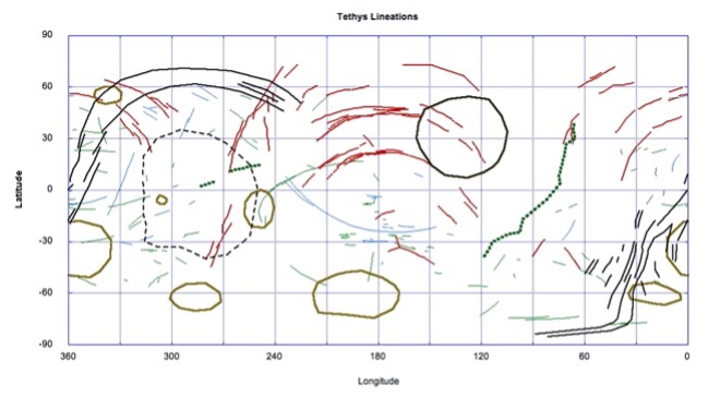
Figure 3: Global map of fractures, ridges, and lineations on Tethys. IR lineations are shown in red. Odysseus is large circle at upper center.
1.1 IR-Lineations
There are at least three prominent sets in the northern anti-Saturn hemisphere, centered on the anti-Saturn meridian (Fig. 3). Each setconsists of ~5–10 parallel lineations a few kilometers across and 50–250 km long. The lineations are remarkably curvilinear (i.e., non-sinuous), do not follow great circles, and are not deflected by major impact structures: they cross the floor of the 400-km-diameter, 9-km-deep Odysseus impact basin as if it were not there.
Although more poorly observed, sub-Saturn hemispheric color imaging at low-phase angle clearly shows a similar set of arcuate, reddishlineations on that hemisphere, despite deposition of E-ring dust particles from Enceladus [2] indicating that these features are being renewed on some time-scale.
The red lineaments centered near ~25° N, 175°E were imaged at high resolution. Mapping at ~90–125 m/pixel (Fig. 4) (together with stereo andlower resolution color imaging) shows no discrete scarp, ridge, or other tectonic manifestation along the ~100 km portion of the feature soimaged. Only a faint discoloration of the surface has been identified (Fig. 5). Further, >20 dark spots 200–800 m in diameter lie along this setof lineaments. These spots are characterized by very low albedos, sharp boundaries, and no evidence of raised rims consistent with an impactorigin. Of these, >60% are situated at the bottom of impact craters.

Figure 4: High-resolution, 90 m/pixel mosaic of IR lineaments, merged with IR3–Gr–UV3 color mosaic.

Figure 5: Enlargement of high-resolution view in Figure 4 showing reddish lineament (red arrows) and small dark spots (blue arrows).
Red streaks centered at 45° N, 333°E were targeted for high resolution ISS and VIMS observations in late 2015 (although the VIMS cubes were partially corrupted). As at the above site no discrete faults, scarps or grooves was resolved here despite pixel scales as good as ~60 m.
- 2. Origin of IR-Lineaments
The spatial pattern of IR lineaments on Tethys shows a strong symmetry (Fig. 3), centered on the current tidal axis with Saturn. A lack ofcorrelation with local geology might suggest an exogenic origin. Conversely, there are no rayed craters at the radial centers of these features.Further, the locations of the patterns on both the sub- and anti-Saturn hemispheres, and the lineaments’ parallel orientations, argue against adisrupted comet origin (à la SL9). The lineaments have no systematic orientation relative to Odysseus, indicating that stresses arising fromthe relaxation of that basin [3] are not responsible for these features.
Global stresses might have produced the pattern we observe. The IR lineaments may match patterns of strain predicted to result from a non-synchronous rotation stress state, although this is unlikely for a cold, triaxial body like Tethys. The best-fit patterns correspond to a combination of global expansion with true polar wander or tidal axis reorientation (Fig. 6a, b). The misfit for global expansion combined recession is significantly larger (Fig. 6c). The dramatic lack of such features in the southern hemisphere (Fig. 3), where only a few short isolated red streaks are evident, is not explained by any currently considered stress regime.
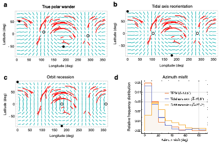
Figure 6: (a-c) Observed (red) and predicted (green) tectonic patterns due to combination of global expansion with (a) true polar wander, (b) tidal axis reorientation, (c) orbit recession. Solid and open circles indicate location of initial rotation and tidal axes. (d) Relative frequency distribution of misfit between observed and predicted fault segment azimuths for processes in panels a-c. Labels show mean misfit for each model.
The lack of obvious tectonic deformation despite the strong color signature is unusual (although features may exist below the currentresolution limit). The lineaments could be reactivated ancient fractures, producing a temporal discoloration. At present there is no topographic or morphologic signature to support this. If tectonic, the lineaments might be still forming, with deformation only on a scale below that which we can resolve.
The dark and reddish coloration could be due to a particulate contaminant in the ice grains that is more spectrally visible if the grain sizes are larger along the streaks. Alternatively, a dark reddish contaminant has been deposited on the surface along the streaks. Such a contaminant could be due to precipitation of a distinct material along unresolved surface or near-surface fractures, with subsequent mixing of contaminant into the local regolith. VIMS spectral cubes are being reprocessed to verify whether organic rich materials may be involved. Low-volume but persistentoutgassing and emplacement of volatiles from the interior (possibly due to clathrate decomposition associated with fracture formation) thecolors of which are distinct from the evolved surface and/or result from alteration due to exposure to the space environment, may be responsible.
The coloration of Tethys unique red streaks, and collocated dark spots, are consistent with active alteration of the surface, given that E-ringaccumulation is expected to remove intrinsic color signatures in a geologically short time period. Differences in particle sizes of the outgassed material may add to this spectral distinctiveness.
How to cite: Schenk, P., Buratti, B., Clark, R., Byrne, P., McKinnon, W., Matsuyama, I., Nimmo, F., and Scipioni, F.: Red Streaks on Tethys: Evidence for Recent Activity, Europlanet Science Congress 2022, Granada, Spain, 18–23 Sep 2022, EPSC2022-732, https://doi.org/10.5194/epsc2022-732, 2022.
Io is the innermost galilean satellite of Jupiter and object to extreme tidal forces. As a result of these forces Io is the most volcanically active body in our solar system. Its large volcanic plumes can rise up to several hundred kilometres above the surface and are one known source of Io's SO2 atmosphere. Additionally, the surface of the moon is covered with surface frost which sublimates in sunlight and condenses during the night or when Io enters eclipse behind Jupiter. Therefore, Io’s atmosphere is a result of the combination of volcanism and sublimation, but it is unknown exactly how these processes work together to create the observed atmosphere. That is why we want to present an approach on modelling Io’s atmosphere and provide a better understanding of the ongoing dynamic processes.
Both, the gas flow of the plume and the sublimation atmosphere, are modelled using the Direct Simulation Monte Carlo (DSMC) method first utilised by G. A. Bird [1]. The DSMC method is the most suitable for this case because the gas dynamics can be modelled over a great range of gas densities which is especially important for rarefied gas flows at high altitudes and on the night side of Io. It is a particle-based method which returns a 3D gas flow field as a result. While we currently focus on single species simulations, our DSMC code is designed to support multiple species enabling us to study the gas emission of other volcanic features as for example lava lakes in the future. This allows us to investigate the influence and contributions of different processes to the atmosphere. The idea of our work is based on simulations done by McDoniel et al. [2].
In a first case, we are investigating the flow of SO2 gas from the source of a plume, into the umbrella-shaped canopy and eventually back onto the surface locally. Additionally, we also study the interaction of the plume with an ambient sublimation atmosphere. In a second case, data obtained by the Galileo SSI experiment is used to create a surface albedo map of Io which enables us to calculate a more precise global thermal model for the sublimation atmosphere. We can then place plumes on the surface and study the interaction of volcanic and sublimation effects globally. Finally, we are also able to implement dust particles in the plume and analyse the effect for different dust sizes. From these results we can calculate images of the column density and the reflectance which in a next step could be used to compare to observational data.
Overall, our goal is to gain a better understanding of the plume structure, the interaction with the ambient atmosphere and the overall contribution of different processes to Io's atmosphere in preparation for future missions such as JUICE, Europa Clipper and a possible future Io Volcano Observer.
[1] Bird, G. A. (1994). Molecular Gas Dynamics and the Direct Simulation of Gas Flows.
[2] McDoniel, W. et al. (2019). Simulation of Io’s plumes and Jupiter’s plasma torus. Phys. Fluids 31, 077103. DOI: 10.1063/1.5097961.
How to cite: Klaiber, L., Thomas, N., Marschall, R., and Milazzo, M.: DSMC Simulations of Io’s atmosphere, Europlanet Science Congress 2022, Granada, Spain, 18–23 Sep 2022, EPSC2022-931, https://doi.org/10.5194/epsc2022-931, 2022.
OPS6 | Aerosols and clouds in planetary atmospheres
Abstract
We present Doppler wind velocity final results of Saturn’s zonal flow at cloud level. Our aim is help to constrain the characterization of the equatorial jet at cloud level and the latitudinal variation of the zonal winds, to measure its spatial and temporal variability, to contribute to monitor the variability in order to achieve a better understanding of the dynamics of Saturn’s zonal winds (Sánchez-Lavega et al. 2003, 2007, 2016); Finally, the complementarity with Cassini, providing an independent set of observations.
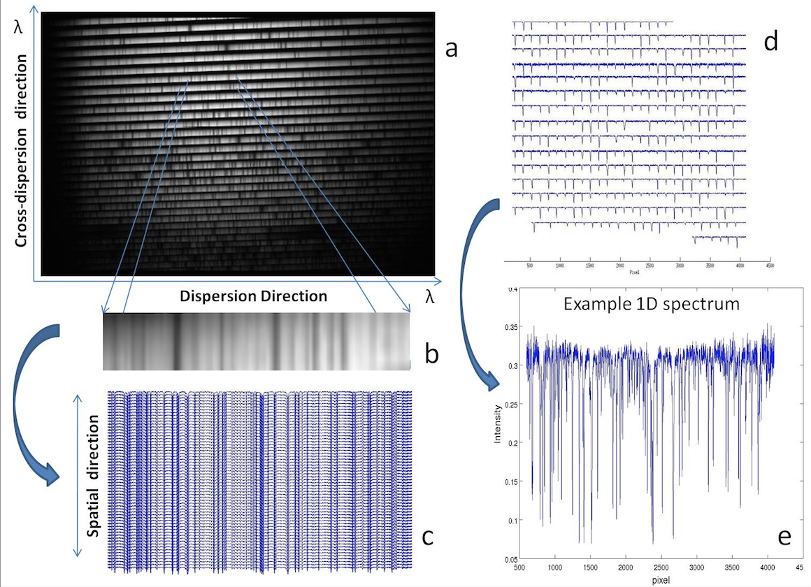
Figure 1: (a) Raw echellogramme showing the spectral orders for one of the detectors. (b) Magnification of part of one order, where absorption lines (dark vertical bands) are visible. From each order, a stack of 61 spectra are extracted. (c) Set of 61 spectra, with each one corresponding to one pixel in the slit’s active window. (d) Each spectrum is divided into 16 orders in the MIT detector and 23 orders in the EEV detector. The plot shows an example of the 16 components of an MIT spectrum, each coming from one spectral order. (e) Example spectrum from one order and one location in the Venus disk. Machado et al. (2012).
The study of the planet’s global system of winds at the 0.7 bar region is based on high resolution spectra from the UV-Visual Echelle Spectrograph (UVES) instrument at ESO’s Very Large Telescope (VLT). Under the assumption of predominantly zonal flow, this method allows the simultaneous direct measurement of the zonal velocity across a range of latitudes and local times. The technique, based on long slit spectroscopy combined with the high spatial resolution provided by the VLT, has provided the first ground-based characterization of the latitudinal profile of zonal wind in the atmosphere of Saturn and the first zonal wind field map in the visible. It promises to improve the characterization of the equatorial jet and the latitudinal variation of the zonal winds, as well the measurement (and monitorization) of its spatial and temporal variability, achieving a better understanding of the dynamics of Saturn’s zonal winds (which Sánchez-Lavega have found to have changed in recent years). A complete characterization of the dynamical behaviour of Saturn atmosphere is crucial for understanding its driving mechanisms. Finally, the complementarity with Cassini, has provided an independent set of observations to compare with and help validate the method. The zonal wind profile retrieved is consistent with previous spacecraft measurements based on cloud tracking, but with non-negligible variability in local time (longitude) and in latitude.
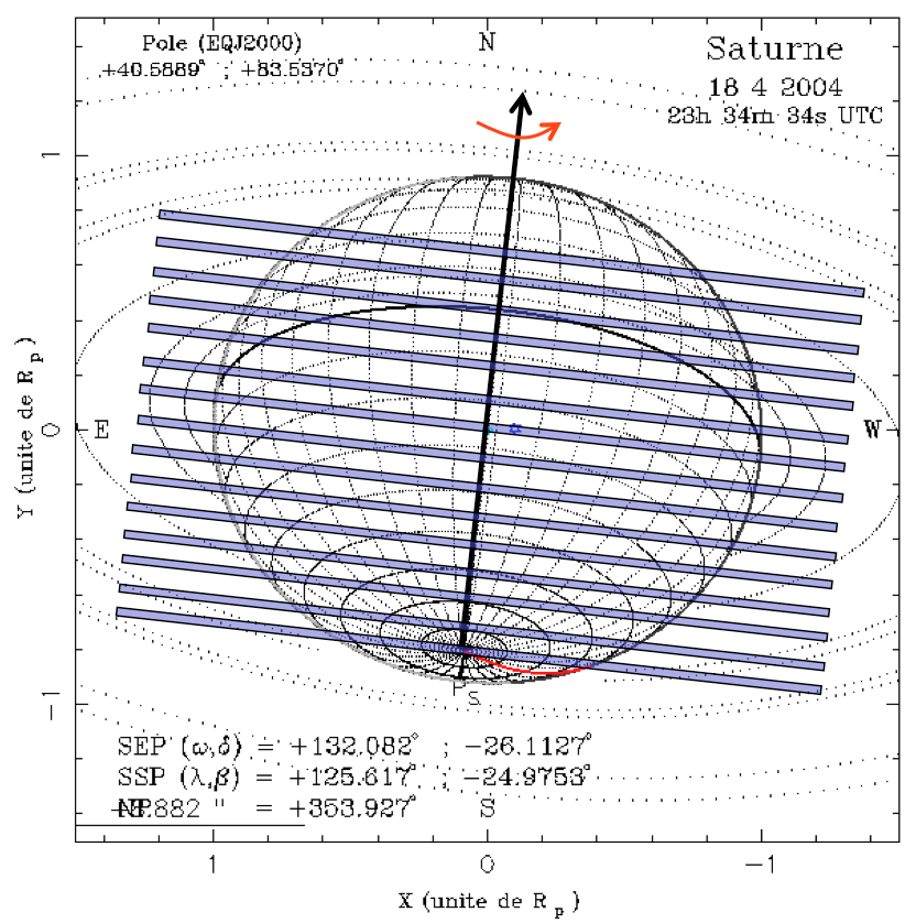
Figure 2: Geometry of the slit positions at the observation days. Saturn’s diameter is 17.4", and the slit aperture is 0,3”x25” . The aperture offset between consecutive exposures is 1". The sub-terrestrial point is at -26.1ºS.
The UVES/VLT instrument has been used, which simultaneously achieves high spectral resolving power and high spatial resolution. The field has been derotated in order to have the aperture aligned perpendicularly to Saturn’s rotation axis. In this configuration, spatial information in the East-West direction is preserved in a set of spectra in the direction perpendicular to dispersion. Our Doppler velocimetry method is based on the technique of absolute accelerometry (Connes, 1985) which has been applied to the backscattered solar spectrum in order to determine the Doppler shift associated with the zonal circulation. Our measurements have been made in the wavelength range of 480-680 nm. Previously we successfully adapted and fine tuned this Doppler velocimetry technique for measuring winds at Venus cloud tops (Machado et al. 2012, 2014,2017, 2021; Gonçalves et al., 2020). In the present study we will show the adaptation of this method for Saturn’s case. We will use coordinated observations from the Cassini’s Visible and Infrared Mapping Spectrometer (VIMS), in order to compare with the Doppler winds obtained from the UVES/VLT high-resolution spectra.
The observations consisted of 4 blocks of 15 exposures of 90 sec, plus two shorter blocks of 9 exposures, totaling 7.3 hours of telescope time. In order to cover the whole disk the aperture has been offset by 1 arcsec in the North-South direction between consecutive exposures. Most of the northern hemisphere was covered by the rings. Saturn’s diameter was 17.4 arcsec, and the slit aperture was 0.3x25 arcsec. The aperture offset between consecutive exposures was 1 arcsec. Two shorter observations blocks of 9 exposures only covered the central part of the disk, and four others covered the whole disk. The sub-terrestrial point was at -26.1 S. The presence of the rings lead to severe order superposition. The dark region between the rings and the disk may or may not be present, depending on the slit position. On the other hand, defects in the response of the UVES slit in the upper part preclude its use for accurate Doppler measurements such as these. For these reasons only the central part of the aperture has been considered for the measurements.
It can be easily noticed that we were able to reproduce with a significant agreement the amplitudes of the wind velocities previously observed in a vast range of latitudes and that they are highly consistent with the cloud tracking measurements from almost simultaneous Cassini data.
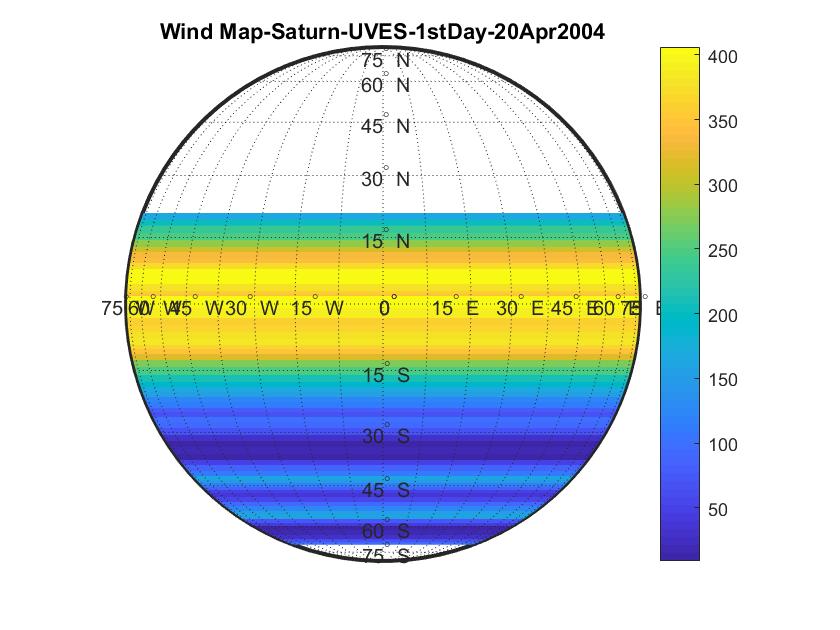
Figure 3: Contour map of Saturn disk for the first night of observations. The wind velocities have units of m/s. Thecolor scale was arbitrary.
References
Connes, P., Absolute Astronomical Accelerometry, Astrophysics and Space Science (ISSN 0004-640X), volume 110, no. 2, p.211-255, 1985.
Goncalves, R., Machado, et al., Icarus, 335, article id. 113418, 2020.
Machado, P., Luz, D.Widemann, T., Lellouch, E.,Witasse, O, , Icarus, Volume 221, p. 248-261, 2012.
Machado, P., Widemann, T., Luz, D., Peralta, J., Icarus, 2014.
Machado, P., Widemann, T., Peralta, J., Gonçalves, R., Donati, J-F., Luz, D., Icarus, 285, 8-26, 2017
Machado, P., et al., Atmosphere, 12, 506, 2021.
Sánchez-Lavega, A., et al., Nature, 423, 623-625, 2003.
Sánchez-Lavega, A., Hueso, R.; Pérez-Hoyos, S., Icarus, 187, 510-519, 2007.
Sánchez-Lavega, A., et al., Nature Communications, 7, id. 13262, 2016.
How to cite: Machado, P., Silva, M., Sánchez-Lavega, A., Silva, J., Espadinha, D., Brasil, F., and Ribeiro, J.: Saturn atmosphere's winds with VLT/UVES Doppler velocimetry, Europlanet Science Congress 2022, Granada, Spain, 18–23 Sep 2022, EPSC2022-354, https://doi.org/10.5194/epsc2022-354, 2022.
Titan’s atmosphere includes many trace hydrocarbon and nitrile species that reach their condensation temperatures in the stratosphere. These, for the most part, will condense out as ices given sufficient condensation nuclei, which are provided by the organic haze particles. Barth (2017) explored the physics behind the size and abundance of pure ice particles that could be present in Titan’s atmosphere and found they would condense out in layers between about 80 and 60 km given thermal conditions at the Huygens landing site (Fig. 1).
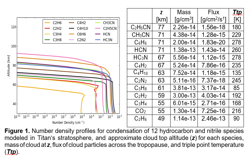
We now expand that study to multiple latitudes and include mixtures of trace species in the ice particles. Anderson et al. (2018) have shown that in Titan’s stratosphere, where many of the trace gases are saturated at the same altitude, they are likely co-condensing onto the haze particles. This changes the optical properties of the particles, but microphysically the formation process is similar to modeling the pure ices, as long as the vapor pressures are adjusted for the mixture.
Modeling is done using the Community and Aerosol Radiation Model for Atmospheres (CARMA; Barth 2020). CARMA models the physics of vertical transport and coagulation in a column of atmosphere and the interaction of particles and gases through nucleation, condensation, and evaporation. The growth routines have been modified to include particles composed of multiple volatiles, with each volatile component growing or evaporating in response to the environment (Barth & Toon, 2006). Particles are represented by a number of discrete mass bins, such that the size distribution of ice particles can be explored at all altitudes in the column. The model keeps track of the changes with time of the number of particles (including core mass for clouds) and mass density of volatiles.
This work is supported by NASA CDAP 80NSSC20K0485.
References: Anderson, C. M., R. E. Samuelson and D. Nna-Mvondo 2018. Organic ices in Titan’s stratosphere. Space Sci. Rev. 214, 125; Barth, E.L. 2020. PlanetCARMA: A New Framework for Studying Planetary Atmospheres. Atmosphere, 11(10), 1064; Barth, E. L. 2017. Modeling survey of ices in Titan’s stratosphere. Planet. Space Sci. 137, 20–31; Barth, E. L., and O. B. Toon 2006. Methane, ethane, and mixed clouds in Titan’s atmosphere: Properties derived from microphysical modeling. Icarus 182, 230–250.
How to cite: Barth, E. L.: Microphysical modeling of mixed composition ices in Titan’s stratosphere, Europlanet Science Congress 2022, Granada, Spain, 18–23 Sep 2022, EPSC2022-765, https://doi.org/10.5194/epsc2022-765, 2022.
We have determined the real and imaginary refractive indices (n and k, respectively), from the visible to the near infrared (0.4 to 1.6 µm), of five laboratory-generated organic refractory materials produced from gas-phase chemistry with the NASA Ames COSmIC facility. The solid samples were produced using a plasma discharge in the stream of a 200-K supersonic jet-cooled expansion of different gas mixtures to study the impact of the molecular precursors on the solid sample optical properties. Three samples were produced from N2:CH4 (95:5) gas mixtures using three different high voltages (700V, 800V and 1000V) to vary the energy in the plasma discharge. One sample was produced from a N2:CH4:C2H2 (94:5:5:0.5) gas mixture, with a high voltage of 1000 V. The fifth sample was produced in an Ar:CH4 (95:5) gas mixture with a high voltage of 1000 V to produce a nitrogen-free hydrocarbon sample. The optical constants, n and k, of these five samples were determined using spectral reflectance measurements. They appear to be positively correlated with the nitrogen content in the solid sample, i.e., a sample with larger nitrogen content exhibits higher n and k values.
We have used these refractive indices as input parameters in a radiative transfer model to analyze Cassini Visible Infrared Mapping Spectrometer (VIMS) observations of Titan’s atmosphere. The results show that using the tholin samples with higher n and k values (higher nitrogen content) provides a better fit to the observational data than using the samples with lower n and k values (lower nitrogen content). The Titan tholins with higher nitrogen content therefore appear to be more representative of the Titan aerosols observed by VIMS.
How to cite: Sciamma-O'Brien, E., Roush, T., Rannou, P., and Salama, F.: First Optical Constants from 0.4 to 1.6 µm of Titan Aerosol Analogs Produced in the NASA Ames COSmIC Facility and Their Use in a New Analysis of Cassini VIMS Observations, Europlanet Science Congress 2022, Granada, Spain, 18–23 Sep 2022, EPSC2022-1199, https://doi.org/10.5194/epsc2022-1199, 2022.
MITM5 | Machine Learning in Planetary Sciences
Evidence of explosive volcanism on the surface of Mercury has been identified in the form of vents and pyroclastic deposits using images and spectral data acquired by the MESSENGER mission (Goudge et al. 2014, Thomas et al. 2014, Jozwiak et al. 2018, Pegg et al. 2021). Understanding the history of the volcanic eruptions forming these features provides an insight in the geological and thermal evolution of the planet. To this end, it is important to constrain the characteristics of each vent and, correlating them with the environment, classify the features according to their age and geological conditions. An individual analysis of a selection of vents has been carried out by Barraud et al. 2021 and Besse et al. 2015, providing new insights on the size, volcanic content and spectral properties of these features. However, performing a global analysis presents further challenges. The collection of volcanic features identified presents a wide variety of characteristics in terms of morphology (simple vent, pit vent, vent-with-mound etc.), shape (circular, elliptical, curved), location (crater centre, crater rim, inter-crater plain), distribution (isolated or compound) and spectral properties of the pyroclastic deposit. This introduces a large number of variables that complicate the characterisation and timing of volcanic eruptions.
The vast amount of data returned by the MESSENGER mission offers both a challenge and an opportunity in the methodology to solve this problem. While the combination of a large number of observations from different instruments can complicate the physical interpretation of a given process, it opens the door to the use of machine learning techniques. These methods rely on the identification of patterns on the input data without considering the associated physics, with the aim to reveal underlying correlations that can then be related to physical and chemical phenomena. This technique has been applied to the entire dataset collected by the Mercury Atmospheric and Surface Composition Spectrometer (MASCS), to classify the visible-near-infrared reflectance spectra into three categories (D'Amore et al. 2022).
In this work, we investigate the application of machine learning to explore the differences amongst the pyroclastic deposits and volcanic vents, with the aim of improving the understanding on the evolution of explosive volcanism in Mercury. In this methodology we combine data from the MASCS and the Mercury Laser Altimeter (MLA) instruments with other properties of the vent surroundings (e.g., crustal thickness). By treating unrelated physical variables together as components of the same input vector, the outcome is a set of dimensions that have no direct physical meaning but can uncover underlying structures to be later physically or chemically interpreted.
How to cite: Leon-Dasi, M., Besse, S., and Doressoundiram, A.: Exploring the diversity in pyroclastic deposits and volcanic vents on Mercury with machine learning techniques, Europlanet Science Congress 2022, Granada, Spain, 18–23 Sep 2022, EPSC2022-680, https://doi.org/10.5194/epsc2022-680, 2022.
InSight seismic data and marsquake catalogue
NASA's InSight seismometer has been recording the seismicity of Mars for over 3 years and to date, over 1300 seismic events were found by the Marsquake Service (MQS) [1,2]. Marsquakes usually have a low signal-to-noise ratio (SNR) and are consequently often hidden or contaminated by the background noise, making their detection and analysis challenging. Local winds interact with the lander and seismometer system and generate noise levels that fluctuate throughout the Martian day and regularly exceed typical event amplitudes. Additionally, extreme temperature changes cause transient high-amplitude spikes [3]. Conventional tools, such as the STA/LTA detectors, perform poorly on this dataset, as the various noise signals often share a common bandwidth and can be similar in duration to marsquakes [3]. Therefore, MQS detects events by manual data review and discriminates them from wind noise [4] by comparing the seismic data to onboard wind measurements if available, or otherwise, to the excitation of wind-driven lander modes. MQS classifies events by their frequency content into low- (<10%) and high-frequency (>90%) event families and assigns a quality based on their locatability (A: highest to D: lowest quality) [1].
Marsquake detection with convolutional neural network
Deep learning methods, and in particular convolutional neural networks (ConvNet) are nowadays routinely used for complex tasks such as speech or visual object recognition [5]. Here, we use a ConvNet architecture designed for image segmentation [6] to detect marsquake energy in the time-frequency domain. We train the ConvNet to predict segmentation masks that pixel-wise identify event and noise energy based on the time-frequency representation of a given waveform. We use the method to detect marsquakes and to decompose their signal in event and noise components. This allows us to estimate the marsquake duration, frequency content, and SNR. We use the ConvNet to extend the MQS catalogue and further highlight its value in removing noise contamination from marsquakes [7]. Since the MQS catalogue is much smaller than typically labelled datasets used in deep learning [7], we create a training set with synthetic events with stochastic waveform modelling [8]. Synthetic events mimic the different MQS event types in terms of frequency content and duration and are combined with recorded InSight noise to include all types of noise.
Results
We run our ConvNet-based detector on the complete 20 samples-per-second dataset (over 900 Martian days) and compare our results to the careful manually curated MQS catalogue: we can detect all high-quality events and the majority of low-quality events - in addition to these, we find many additional low SNR events. We extend the catalogue by ~50% more events, of which the majority belongs to the high-frequency event family. An overview of the MQS events and our new detections is given in Figure 1. Similar to the MQS catalogue, we find many events in the quiet evening periods during the spring and summer of the Martian year 1 and 2, and further increase the number of events during the nights when noise levels are elevated. During the high noise periods (day time and winter), when noise amplitudes are orders of magnitudes above typical event amplitudes, we do not confidently detect events apart from a few that fall into short quieter periods. Our results suggest that the MQS catalogue is essentially complete for high SNR events and further support previous findings [9] on the seasonality of high-frequency events and their increased activity in Martian year 2 compared to year 1.
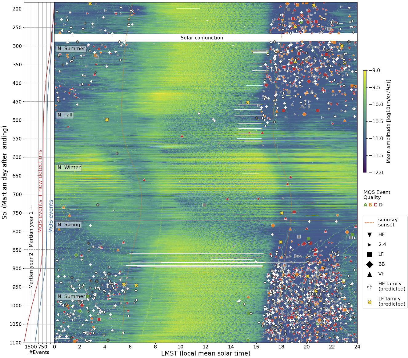
Figure 1: Overview of seismic noise, catalogued MQS events and new detections from ConvNet: the background of the main figure represents the broadband, vertical component seismic noise level (data gaps shown in white). The symbols indicate different event types belonging to the low frequency (LF, BB) or high frequency family (2.4, HF, VF), and colours indicate the qualities in the MQS catalogue; new detections found with our ConvNet detector are shown with their predicted event family type. The panel on the left side shows the cumulative event count using MQS events (blue) and MQS events and new detections (red). The event numbers are dominated by the high frequency events (corresponding to over 90% of events).
References:
[1] Clinton et al. (2021), 10.1016/j.pepi.2020.106595
[2] InSight Marsquake Service (2022), doi.org/10.12686/a16
[3] Ceylan et al. (2021), 10.1016/j.pepi.2020.106597
[4] Charalambous et al. (2021) 10.1029/2020JE006538
[5] LeCun et al. (2015), 10.1038/nature14539
[6] Ronneberger et al. (2015), 10.1007/978-3-319-24574-4_28
[7] Zhu et al. (2019), 10.1109/TGRS.2019.2926772
[8] Boore (2003), 10.1007/PL00012553
[9] Knapmeyer et al. 10.1016/j.epsl.2021.117171
How to cite: Dahmen, N., Clinton, J., Meier, M.-A., Stähler, S., Kim, D., Stott, A., and Giardini, D.: A Deep Marsquake Catalogue, Europlanet Science Congress 2022, Granada, Spain, 18–23 Sep 2022, EPSC2022-1066, https://doi.org/10.5194/epsc2022-1066, 2022.
MITM6 | Planetary space weather
On March 12, 2012, a Coronal Mass Ejection (CME) was released from the Sun with a speed of ~2000 km/s. The CME source region was surrounded by three different coronal holes (CHs), located to the East (negative polarity), South-West (positive polarity) and West (positive polarity). Its interplanetary counterpart (ICME) impacted Earth and was in-situ measured by the Advanced Composition Explorer (ACE) / Wind at L1 and the Solar TErrestrial RElations Observatory Ahead (STEREO)-A on March 15th. During this period, the angular separation between the two locations was greater than 100 degrees. Nevertheless, the in-situ measurements revealed almost identical profiles with clear markers of ICME signatures, which is evidence of one of the widest reported multi-spacecraft detection of an ICME, having STEREO-A crossing the west flank and Earth the east flank. Supra-thermal electrons show signatures of bidirectionality and isotropy/simple strahl as the ICME crosses the different spacecraft, providing information about the eroded parts of the ICME. Certain parts might have been eroded, possibly due to the interaction with the fast solar wind produced by the nearby CHs. We analysed the propagation of the ICME structure using remote-sensing observations from both STEREOs and Earth together with different in-situ instrumentation at ~1 au, and performed a comparison between the physical properties derived at multiple spacecraft. This study shows the importance of multi-spacecraft observations to understand the large-scale structures of ICMEs, their evolution and interaction, as well as their implications for the space-weather discipline.
How to cite: Carcaboso, F., Dumbović, M., Temmer, M., Gómez-Herrrero, R., Heinemann, S., Nieves-Chinchilla, T., Veronig, A., Jercic, V., Rodríguez-Pacheco, J., Dissauer, K., and Podladchikova, T.: Identical Interplanetary Coronal Mass Ejection Signatures with Wide Angular Separation, Europlanet Science Congress 2022, Granada, Spain, 18–23 Sep 2022, EPSC2022-493, https://doi.org/10.5194/epsc2022-493, 2022.
JUICE is ESA’s first large class mission to the outer Solar System. The main objectives of JUICE are to study Jupiter and its space environment with a special focus on Jupiter’s moons Europa, Ganymede, and Callisto, and their potential habitability. In order to fulfil these objectives, the JUICE measurements need to be accurately corrected for any possible perturbations. Here, we present Spacecraft Plasma Interaction Software (SPIS) simulations of the surface charging of JUICE in the solar wind. The results will be used to correct the future JUICE measurements for the impact of the charging.
We have used a solar wind environment model (i.e. a description of the environment covering typical values for parameters such as electron and ion densities, temperatures, and velocities, magnetic field strengths, and EUV flux) for the location where JUICE will perform its first measurements, between 1500 and 3000 RE from Earth. The typical values for the solar wind parameters and the minimum and maximum values from the expected parameter ranges have been used to simulate the interaction in both average and “extreme” solar wind conditions. Here we present the main results from the SPIS simulations: the surface potential of the spacecraft; the potentials at the locations of the particle and field instrumentation such as the RPWI Langmuir probes and the PEP plasma analysers; the electron and ion density at the locations of the RPWI instruments and the PEP plasma analysers; the characteristics of perturbing particle populations such as photoelectron and secondary electron populations produced by the spacecraft itself; and the properties of the ion wake of the spacecraft. The detailed knowledge of the listed parameters will be used to provide accurate analyses of the first in-situ particle and field measurements performed by JUICE.
How to cite: Holmberg, M. K. G., Jackman, C., Taylor, M. G. G. T., Witasse, O., Wahlund, J.-E., Barabash, S., Altobelli, N., Cipriani, F., Déprez, G., and Huybrighs, H. L. F.: Surface charging of JUICE in the solar wind, Europlanet Science Congress 2022, Granada, Spain, 18–23 Sep 2022, EPSC2022-603, https://doi.org/10.5194/epsc2022-603, 2022.
A Micro-Channel Plate (MCP) is a widely used component for counting particles in space. Using the background counts of MCPs on Mars Express and Venus Express orbiters operated over 17 years and 8 years, respectively, we investigate the galactic cosmic ray (GCR) characteristics in the inner solar system. The MCP background counts at Mars and Venus on a solar cycle time scale exhibit clear anti-correlation to the sunspot number. We conclude that the measured MCP background contain the GCR information. The GCR characteristics measured using the MCP background at Mars show features that are consistent with the ground-based measurement in solar cycle 24. The time lag between the sunspot number and the MCP background at Mars is found ~9 months. The shorter-term background data recorded along the orbits (with a time scale of several hours) also show evident depletion of the background counts due to the absorption of the GCR particles by the planets. Thanks to the visible planetary size change along an orbit, the GCR contribution to the MCP background can be separated from the internal contribution due to the β-decay. Our statistical analysis of the GCR absorption signatures at Mars implies that the effective absorption size of Mars for the GCR particles have a >100 km larger radius than the solid Martian body.
How to cite: Futaana, Y., Shimoyama, M., Wieser, M., Karlsson, S., Andersson, H., Nilsson, H., Wang, X.-D., Fedorov, A., Andre, N., Holmstrom, M., and Barabash, S.: Galactic Cosmic Rays at Mars and Venus: Temporal Variations from Hours to Decades Measured as the Background Signal of Onboard Micro-Channel Plates, Europlanet Science Congress 2022, Granada, Spain, 18–23 Sep 2022, EPSC2022-633, https://doi.org/10.5194/epsc2022-633, 2022.
Introduction: Surface sputtering by solar wind (SW) ion irradiation is an important process for understanding the surface and exosphere of airless celestial bodies such as the Moon, Mercury, and asteroids. In addition to SW ion induced sputtering, processes such as photon and electron stimulated desorption and impact vaporization, can also contribute to the exosphere formation around airless bodies. A better understanding of relative contributions of these processes is needed to interpret ground-based and spacecraft observations of the exosphere. Our focus here is on SW ion induced sputtering. Laboratory simulations are both complex and expensive. Hence, theoretical sputtering models are used to study the incoming ions, impacted surface, and sputtered atoms. The most common sputtering models, such as TRIM and SDTrimSP, use the binary collision approximation (BCA) and predict the yield and energy distribution of sputtered atoms, along with the depth of deposition and damage, all as a function of the incoming ion type, impact energy, and impact angle.
Within SDTrimSP there are several inputs that have been applied differently in previous SW sputtering simulations1,2,3. These parameters can influence the simulated behavior of both the target and sputtered atoms. Laboratory data is often readily available for comparison with ion sputtering simulations from monatomic or simple oxide targets, and simulations can closely match experimental sputtering yields over a broad energy range. Comparatively, little work has been done to determine how the simulation parameters should be chosen for more complex targets relevant to planetary surface analogs. It is therefore of great interest to understand how sensitive sputtering behavior is to these inputs and what parameter choices best approximate SW sputtering. We have conducted a detailed sensitivity study into SDTrimSP parameters to produce a best-practice for simulating SW impacts onto the lunar surface. These results can be used to establish a more consistent methodology for simulations of SW induced sputtering.
Methods: First, we consider the sensitivity of the SDTrimSP simulated SW sputtering behavior to several user input parameters. In all cases we simulated the effect of H or a combination of H and He onto an anorthite (CaAl2Si2O8) surface. Within SDTrimSP we considered the role of the O surface binding energy (SBE), ISBV (the method of dealing with SBEs for compounds), static vs. dynamic simulations, impact energy approximations, incidence energy approximations, and the elemental composition of the SW. For all parameters we quantified their effect on the overall sputtering yield, elemental composition of the sputtering yield, elemental surface concentration, damage production, and energy distribution of sputtered atoms. Based on these sensitivity results we recommend a best-practice for simulating SW sputtering using SDTrimSP.
Results: The predicted sputtering behavior was shown to be highly dependent on several of the SDTrimSP parameters considered. For example, previous SW simulation studies have used O SBEs between 1 and 6.5 eV, based on recommended values, fitting to experiment, and monomatomic sublimation energies. For all cases considered, the O SBE had a significant affect on the overall and elemental yield. Furthermore, dynamic simulations, which allow for the surface to change as a function of fluence, better represent the surface evolution during SW impacts. The effect of the O SBE can also be seen in the surface composition as a function of fluence (Fig 1). For an O SBE of 1 eV, strong preferential sputtering of O is observed, and the surface composition fraction is reduced from 0.6 to 0.3 at a fluence of 200 x 1016 atoms/cm2. In contrast, there is almost no reduction in O surface composition for an SBE of 6.5 eV. This large depletion in surface O at an SBE of 1 eV has not been observed in previous irradiation experiments of silicates4,5,6. Therefore, O SBEs of 1 eV are likely not representative of what would be seen for materials relevant to planetary science.
Varying the ion incidence angle also significantly affected the sputtering behavior. Impacts normal to the surface are often used to simulate a flat surface and can more easily be compared to experimental data. However, the surface of the Moon and Mercury consists largely of approximately spherical weathered grains. As a result, incoming SW ions are impacting the surface at many different relative angles. When oblique incidence angles are simulated the elemental and overall yields increase in all cases. For both cases there was also an increase in the peak of the damage distribution along with a reduction in depth at this peak.
Accounting for the He component in the SW leads to a 20% increase the elemental sputtering yields and and a 20% increase in the damage produced within the substrate (Fig 2). Therefore, while He makes up only 4% of the SW it accounts for over 20% of the sputtering behavior. When comparing the H and H + He options the proportion of O in the yield stays consistent. This suggests that a factor could be used to account for the He contributions.
In summary, while SDTrimSP represents a valuable tool to better understand the effect, the results are highly dependent on many user-specific parameters. This study directly quantifies these sensitivities on the SW-induced sputtering behavior and concludes with the following best-practice recommendation for SDTrimSP simulations of SW sputtering:
- 1 keV/amu impacts (96% H, 4% He) to approximate SW composition
- Dynamic simulations to allow for the behavior to evolve as a function of fluence
- Cosine distribution of impact angles onto the surface to approximate spherical grains
- Incorporation of mineral specific SBEs where possible
References:
1. Mutzke, A., et al. (2019) “IPP-report 2019-02”
2. Szabo, P. S., et al. (2018) doi: 10.1016/j.icarus.2018.05.028
3. Schaible, M. J., et al. (2017) doi: 10.1002/2017JE005359
4. Dukes, C.A., et al. (1999) doi: 10.1029/98JE02820
5. Dukes, C.A., et al. (2015) doi: 10.1016/j.icarus.2014.11.032
6. Laczniak, D.L., et al. (2021) doi: 10.1016/j.icarus.2021.114479
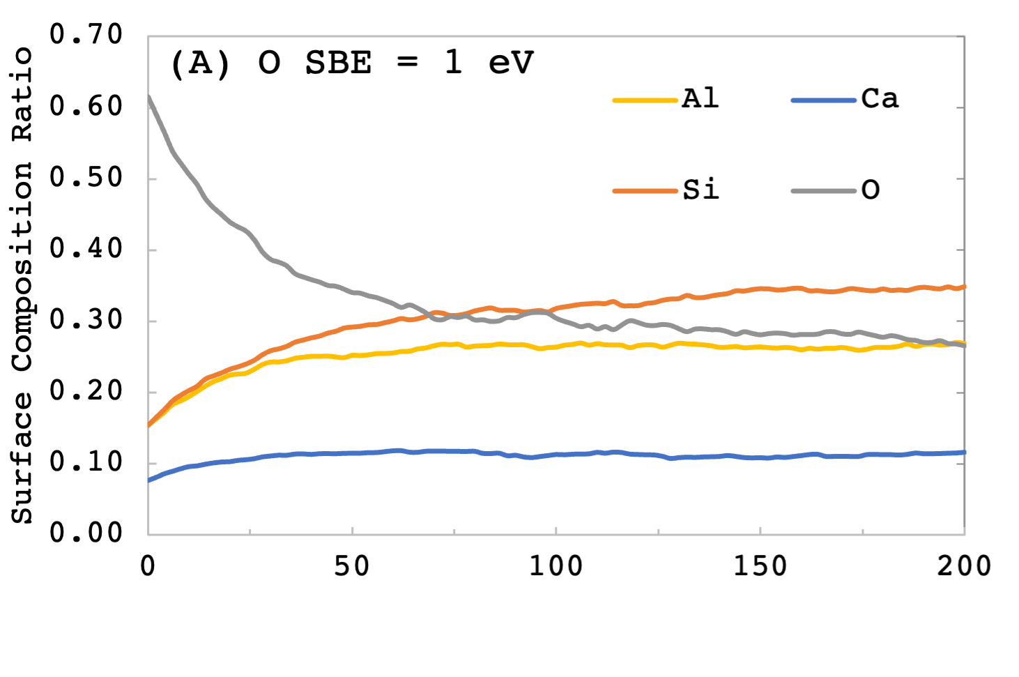
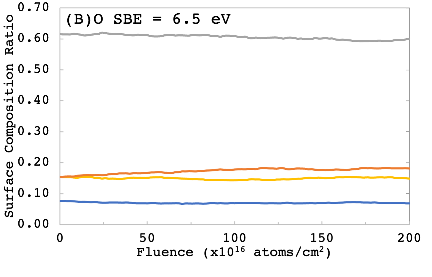
Fig 1. Surface composition as a function of fluence for and O SBE of 1 eV (A) and 6.5 eV (B)
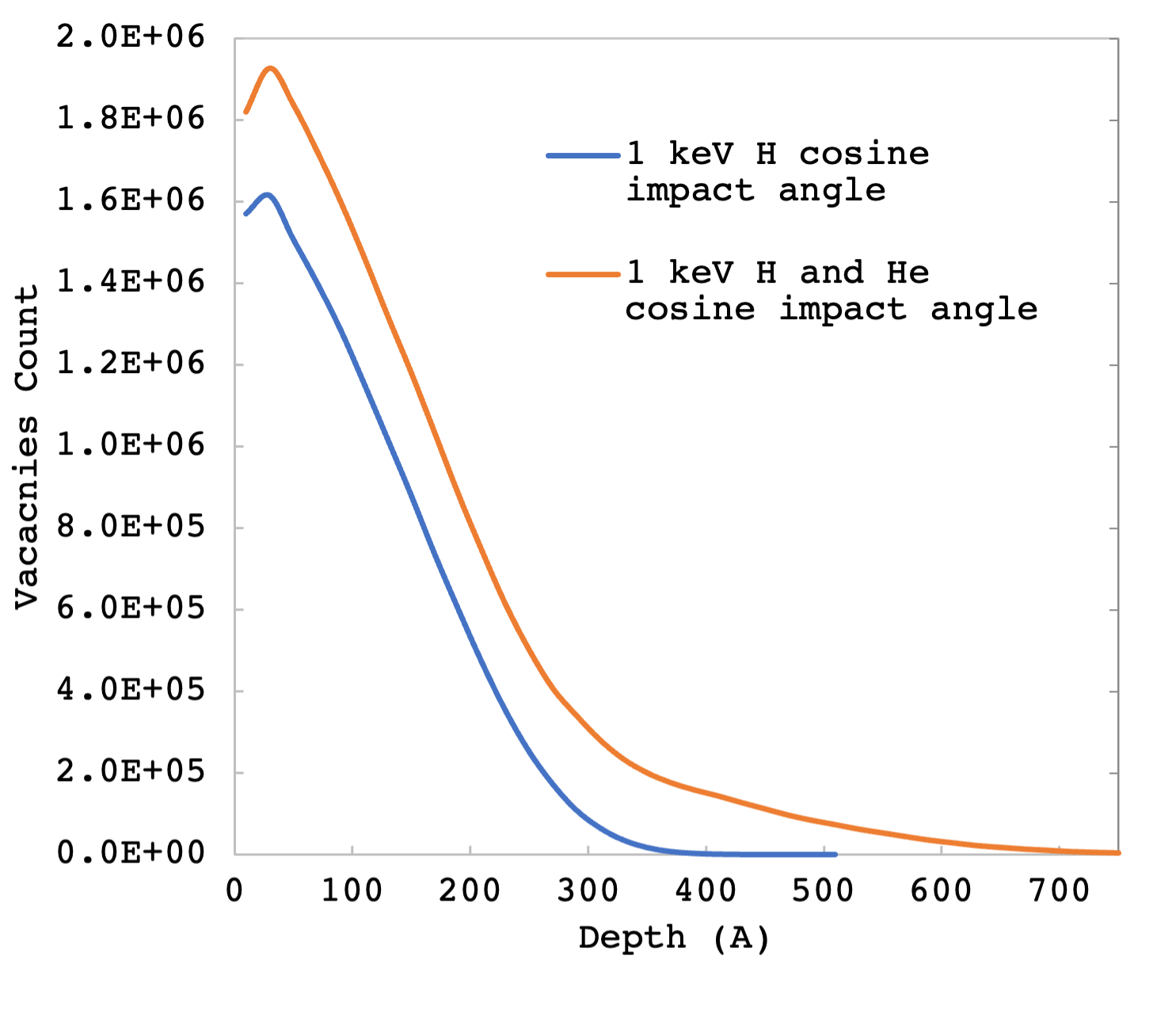
Fig 2. Count of vacancies as a function of depth for different SW compositions using a cosine distribution of the impact flux vs impact angle
How to cite: Morrissey, L., Schaible, M., Tucker, O., Szabo, P., Bacon, G., Killen, R., and Savin, D.: Establishing a Best-Practice for SDTrimSP Simulations of Solar Wind Ion Induced Sputtering, Europlanet Science Congress 2022, Granada, Spain, 18–23 Sep 2022, EPSC2022-723, https://doi.org/10.5194/epsc2022-723, 2022.
We present an overview of the University of Tasmania’s (UTAS) progress in monitoring and providing ground support for space projects. With five radio telescopes distributed across Australia, UTAS has a good capacity to study a wide range of scientific phenomena in our Solar System and to improve the outcome of space missions. High-cadence Mars Express spacecraft observations in the X-band (8.4 GHz) were monitored between 2014 and 2022 using the European Very Long Baseline Interferometry (VLBI) network and UTAS radio telescopes to study interplanetary plasma scintillation and characterise solar wind parameters. The quantification of the plasma’s effect on the radio signal helps in phase referencing for ultra-precise spacecraft tracking. The international collaboration with the China National Space Administration (CNSA) also allowed simultaneous coherent tracking of the interplanetary plasma scintillation for the incoming radio signals of the Mars Express and Tianwen-1 spacecraft.
Space weather monitoring has been carried out to study events such as coronal mass ejections using radio signals transmitted by the Solar Orbiter and Solar Heliospheric Observatory (SOHO) spacecraft. The unique radio telescope infrastructure at UTAS will be essential in providing ground support to the Planetary Radio Interferometry and Doppler Experiment (PRIDE) led by the Joint Institute for VLBI ERIC (JIVE). The PRIDE experiment has been chosen by the European Space Agency (ESA) for the JUpiter ICy Moons Explorer mission (JUICE) that will explore three of Jupiter’s moons: Europa, Ganymede, and Callisto. This space mission is scheduled to launch in April 2023.
In addition, University of Tasmania has been conducting observations with NASA and JPL for bi-static radar tracking experiments to detect and monitor Near-Earth Asteroids. Over 14 observations have been conducting with UTAS radio telescopes since the beginning of 2021.
How to cite: Md Said, N. M., Molera Calvés, G., Kummamuru, P., Edwards, J., and Cimo', G.: Space science advancements at the University of Tasmania, Europlanet Science Congress 2022, Granada, Spain, 18–23 Sep 2022, EPSC2022-774, https://doi.org/10.5194/epsc2022-774, 2022.
MITM7 | Small sensors, instruments and payloads for planetary exploration
The Visual Monitoring Camera (VMC) is a small camera onboard Mars Express, initially intended to provide visual confirmation of the separation of the Beagle 2 lander. In 2007, a few years after the end of its original mission, VMC was turned on again to obtain full-disk images of Mars for outreach purposes (Ormston et al., 2011). As VMC obtained more images, the scientific capabilities of the camera became evident (Sánchez-Lavega et al., 2018), and finally the small camera was upgraded to be a new scientific instrument, with an agreement between the European Space Agency (ESA) and the University of the Basque Country (Spain; UPV/EHU). In this work we describe the calibration and technical efforts that are allowing us to maximize the scientific output from this small camera.
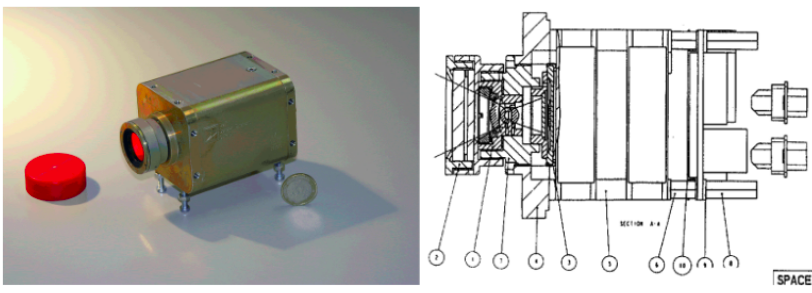
Figure 1. Image of VMC before launch (left) and scheme from the Flight User Manual (right)
VMC is also called the Mars webcam, as it is similar to a typical webcam of the 2000s. The sensor has a a 640x480 pixel array, and a Field of View (FOV) of 30ºx40º. This wide FOV, together with the elliptical orbit of Mars Express, enables full-disk observations from apocenters, which are the most common product of VMC. It is also possible to use this wide FOV to image large sections of the limb, and therefore monitor the occurrence of high altitude aerosols, as shown by Sánchez-Lavega et al. (2018).
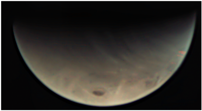
Figure 2. Full disk of Mars as seen by VMC.
Operations
Since 2018 VMC operations follow a similar routine as those used for other science instruments. The Science Ground Segment takes care of the Medium Term Planning (MTP) following the inputs from the science team. The science team performs the Short Term Planning (STP). Fig. 3 shows a typical VMC observation, which consists of a default image, followed by one to several loops of 6 images that use a set of predefined exposures. The exposure times are set to maximize the dynamic range of the final science products obtained by combining the individual images.
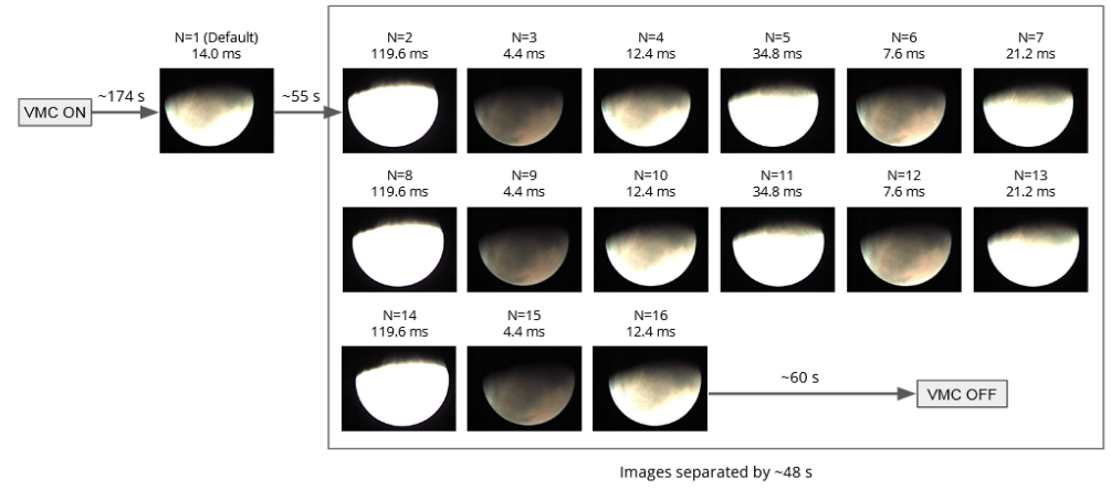
Figure 3. Scheme of a typical VMC observation.
Calibration of images
The images are calibrated following the standard scheme of subtracting a dark current and dividing by a flatfield image. The flat field correction is much more relevant than the dark correction in the quality of the final images after calibration. No onground calibration is known for VMC, therefore the dark current and flat-field corrections used are based only on in-flight observations. The dark was obtained by pointing VMC to the sky, specifically the area of Eridanus, where few bright stars are present.
The flat-field was created using dark-corrected images of flat portions of Mars that were well and uniformly illuminated, as free as possible from large structures, and as flat as possible.
Calibrated images are routinely archived at ESA’s Planetary Science Archive (PSA), as described by Ravanis et al. (2020)
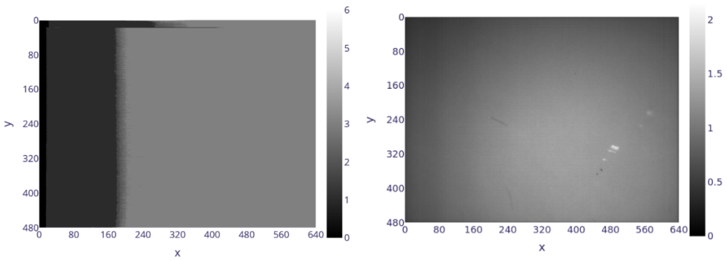
Figure 4. VMC dark (left) and flat (right).
Geometry
The original documents indicate the design parameters for the orientation of VMC in the reference frame of MEX, and for the pixel resolution (iFOV). However, the accurate parameters once VMC was mounted on MEX were never measured on the ground. In addition to this, we find that the timestamp of images suffers a random shift of a few seconds. As a result, we have 5 free parameters: 3 Euler angles for the attitude relative to the MEX reference frame; the pixel resolution (iFOV); and the shift in time from the actual timestamp to the labeled timestamp.
In order to determine the attitude and iFOV of VMC relative to Mars Express, we used images showing stars. Many of these observations covered the stars of the constellation of Orion, because several suitable stars are present in that region of the sky. During these observations the spacecraft maintains a fixed attitude, therefore, the time related uncertainty is not present and only 4 free parameters remain: 3 Euler angles, and the pixel size. These parameters are shown in table 1.

Table 1. VMC geometric parameters as given by the Flight User Manual (FUM) and calibrated values.
The shift in time was estimated from observations showing Phobos. The relative speed of Phobos as seen from Mars Express is high, and therefore it is possible to use its position as an accurate clock. We find that our images are usually obtained between 6 and 13 seconds before the labeled time, but we find random variations. Subtracting 10 seconds is considered a good strategy in most cases, but this uncertainty remains as a limitation.
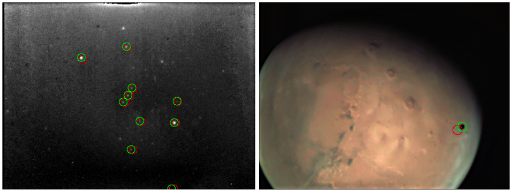
Figure 5. VMC image showing the stars of Orion (left), and Phobos in front of Mars (right). Red circles represent the expected position before calibration. Green circles are the expected positions according to the new calibration.
Conclusions
Within the expectable limitations, the performance of this new instrument is very good and VMC is enabling novel science results and techniques (e.g. Hernández-Bernal et al. 2021). This is in part because VMC provides some capabilities that are not common among instruments in orbital planetary missions. Even with no on-ground calibration available, it has been possible to calibrate the camera, both photometrically and geometrically. Some hardware limitations remain, and others have been partially overcome with specially developed operational strategies.
References
Hernández‐Bernal et al. (2021). A Long‐Term Study of Mars Mesospheric Clouds Seen at Twilight Based on Mars Express VMC Images.
Ormston et al. (2011) An ordinary camera in an extraordinary location: Outreach with the Mars Webcam.
Ravanis et al. (2020). From engineering to science: Mars Express Visual Monitoring Camera's first science data release.
Sánchez-Lavega et al. (2018). Limb clouds and dust on Mars from images obtained by the Visual Monitoring Camera (VMC) onboard Mars Express.
How to cite: Hernández Bernal, J., Cardesín Moinelo, A., Hueso Alonso, R., Ravanis, E., Burgos Sierra, A., Wood, S., Marín Yaseli de la Parra, J., Merrit, D., costa Sitja, M., Escalante, A., Grotheer, E., Esquej, P., Dias Almeida, M., Martin, P., Titov, D., Wilson, C., del Río Gaztelurrutia, T., Sánchez Lavega, A., and Sierra, M.: The Visual Monitoring Camera on Mars Express: calibrating a new science instrument made from an old webcam orbiting Mars, Europlanet Science Congress 2022, Granada, Spain, 18–23 Sep 2022, EPSC2022-684, https://doi.org/10.5194/epsc2022-684, 2022.
Introduction: The camera performance for space missions should be verified before flight. Exposure times with the expected fluxes should be planned, resulting signal-to-noise ratios (SNR) computed, and the overall image quality evaluated. This can be done in a specialized laboratory but having a quick simulation tool to help the design in early phase would be an asset.
We have developed a software based on Blender and Python post-processing for the abovementioned purpose. The software [1] is used with the ASPECT hyperspectral camera (Milani CubeSat, ESA’s Hera mission), the HyperScout hyperspectral camera (Hera mission), and the MIRMIS hyperspectral camera unit (ESA’s Comet Interceptor mission).
Modeling and rendering an asteroid or a comet nucleus: Blender is an open-source rendering software that is widely used in many fields [2]. Capabilities in modeling the 3D geometry and rendering the result makes it also suitable for simulating how an asteroid or a comet nucleus would appear when imaged.
For camera testing purposes, the geometry of the target does not need to be completely correct. It is sufficient that the overall size and shape matches the target, and the surface roughness and boulder distribution are representative. Blender has functions for introducing procedural geometric features randomly on the underlying shape, and we use this to introduce boulders of different sizes on the target. For the overall target shape, either low-resolution models derived from lightcurve or radar observations or high-resolution shape models from previous missions can be used, such as the models for Bennu, Ryugu, or 67P/Churyumov–Gerasi¬menko (see Fig. 1).
We have implemented some common photometric models for the surface material in Blender. Blender has some limitations when compared to other ray-tracers, namely it does not really support custom scattering laws to be implemented. The internal ray-tracing loop employs only Blender’s internal shaders, i.e., scattering laws for a surface element. In other words, one can implement any phase function depending only on the phase angle in Blender, but not disk function that would depend on the incident and scattering directions.
Fortunately, Blender’s internal shaders include Lommel-Seeliger (‘volume scatter’ in Blender) and Lambertian (‘diffuse BSDF’), and one can also mix these, which covers already the common disk functions for dark and bright surfaces quite well. For phase functions we have implemented the exponential-polynomial, linear-magnitude, and ROLO functions as shown in [3]. By combining the disk and the phase functions we can implement Lommel-Seeliger, ROLO, McEwen, and Lambert photometric functions for the target.
The Blender part of our software is outputting ‘ideal’ noiseless images with a given observing geometry, camera field-of-view, detector resolution, and surface albedo. Our post-processing step subsequently introduces the effects originating from the camera and the detector physical capabilities.
Camera performance simulation: The images can be converted to real physical units (I/F, Watts, photons, electron counts on CCD). While the RGB channel values in the Blender images have arbitrary units and scale, one can render a Lambertian disk at backscattering with the same illumination intensity and target-camera distance as in the actual object image. This calibration procedure will give us I/F conversion from the RGB values. Considering the target’s distance to the Sun we can further convert these into radiant flux in Watts.
If we are dealing with a spectral instrument, we need to have a spectral image/datacube. Currently we are not changing the parameters of the photometric function with the wavelength. This implies that the received flux is only linearly dependent on the wavelength-dependent albedo of the target, and that we can just multiply one rendered image with the normalized spectra of the target’s surface material for a spectral datacube.
With spectral flux for each image pixel, we can apply the transmission of the camera optics and the spectral filter (i.e., the Fabry-Perót interferometer in ASPECT and MIRMIS cameras). Watts can be converted into photon counts for each wavelength, and finally the detector quantum efficiency curve can be used to achieve electron elementary charges at the detector.
Once the electron charges per time unit on the detector has been solved, we can introduce a reasonable dark field pattern, dark current noise (Poisson), readout noise (Gaussian), and photon shot noise (Poisson) for a given exposure time. This will give us the final, simulated camera image or a hyperspectral datacube of the target, together with the SNR estimate.
Discussion: The SSO object simulated imaging and camera performance tool can be used to produce expected camera data, with realistic noise, for space mission and instrument design. Especially with (hyper)spectral cameras this tool can be used to verify how different spectral and/or spatial details could be resolved with certain exposures, noise levels, and optics/camera transmissions.
We have started with application to atmosphereless, relatively homogeneous targets such as an asteroid or a comet nucleus. Variability to surface properties (local albedo or color, for example) can be introduced using Blender’s procedural modeling tools. Simple atmospheres and comet gas/dust environments could be added in the future. To some extent, this is what is done in the SISPO project [4]. We verify our results against the NASA Planetary Spectrum Generator [5]. For visualizing views to an asteroid or a comet with a given spacecraft flight path, possibly given with a SPICE kernel, we acknowledge the shapeViewer [6] tool.
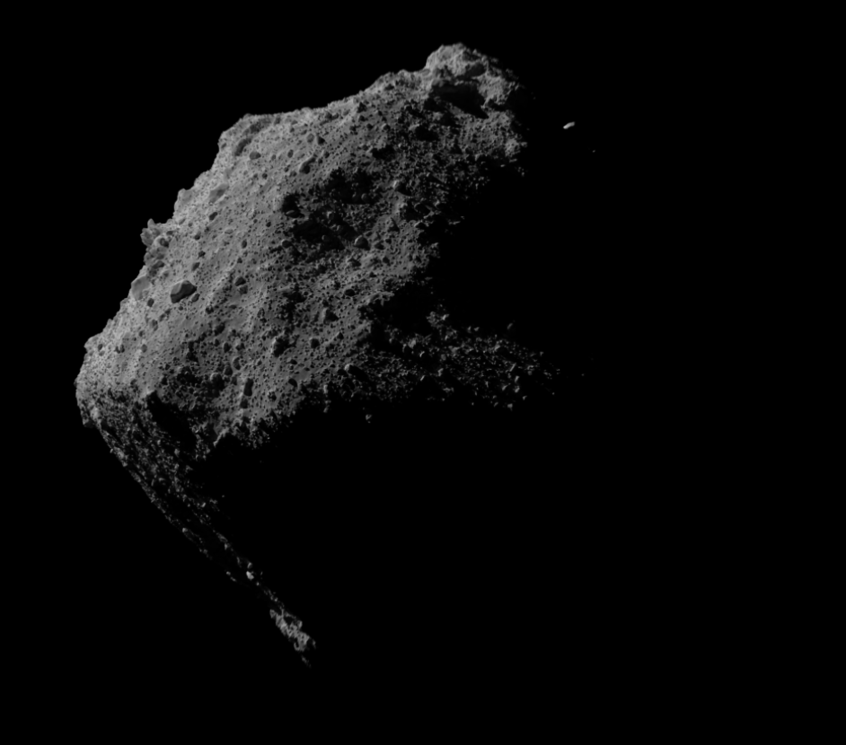
Figure: Blender-visualization of the high-resolution shape model of asteroid Ryugu with added boulders on the surface.
References: [1] Git project for the Blender/Python imaging simulations. https://bitbucket.org/planetarysystemresearch/workspace/projects/SSO_PHOTOMETRY. [2] Blender software, https://www.blender.org/. [3] Golish D. R. et al. (2021) Icarus, 357, 113724. [4] Pajusalu M. et al. (2021) arXiv, astro-ph.IM, 2105.06771. [5] NASA Planetary Spectrum Generator, https://psg.gsfc.nasa.gov/ [6] Vincent J.-B. (2014) ACM conference, Helsinki.
How to cite: Penttilä, A., Palos, M. F., Näsilä, A., and Kohout, T.: Blender modeling and simulation testbed for solar system object imaging and camera performance, Europlanet Science Congress 2022, Granada, Spain, 18–23 Sep 2022, EPSC2022-788, https://doi.org/10.5194/epsc2022-788, 2022.

Introduction:
MiniPINS is an ESA study to develop and prototype miniaturised surface sensor packages (SSPs) for Mars and the Moon. The study aims at miniaturising the scientific sensors and subsystems, as well as identifying and utilizing commonalities between Mars and Moon SSPs, allowing to optimise the design, cut costs and reduce the development time.
Mars In-Situ Sensors (MINS) is a penetrator with approx. 25 kg mass, piggy-backed by another Mars mission spacecraft to Mars. In total 4 identical penetrators are deployed to different landing sites either from the approach orbit or Mars orbit. The design of MINS has significant heritage from FMI’s MetNet mission design[1]. The entry, descent and landing sequence of MINS is completely autonomous and controlled by its on-board computer. In the Martian atmosphere the penetrators undergo aerodynamic braking with inflatable breaking units until they reach the target velocity of 60-80 m/s for entering the Martian surface. The nominal mission duration is one Martian year.
Lunar In-Situ Sensors (LINS) is a miniature 7 kg station deployed on the Moon surface by a rover. LINS mission consist of 4 surface stations deployed to different sites within the rover’s traveling perimeter. The LINS scientific package consists of several scientific instruments to study the Moon for 2 years.
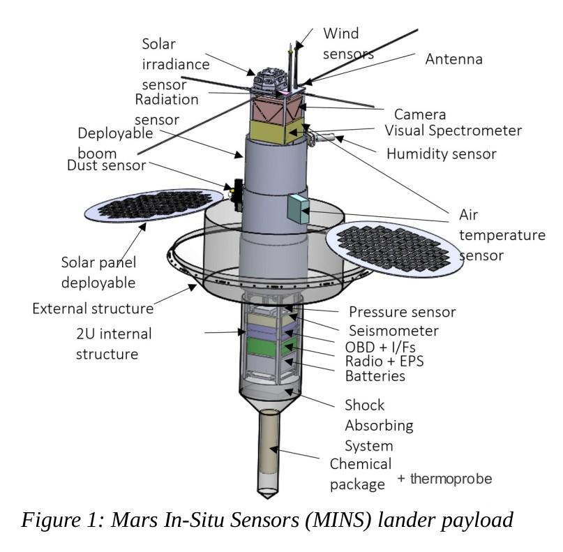
Mars SSP sensors:
MINS will study the Martian atmosphere, seismology and chemistry. The MINS payload consists of a camera, a visual spectrometer, a meteorological package, an impact accelerometer, soil thermoprobes, a chemistry probe, a seismometer and a radiation monitor. Many of the instruments have Mars heritage but additional qualification is required due to landing shock.
The meteorological package consists of air temperature sensors, pressure sensor, relative humidity sensor, wins sensors, dust sensor and solar irradiance sensor. Pressure and humidity sensors are provided by FMI and the sensors have heritage from multiple Mars missions like the M2020 Perseverance rover[2]. Air temperature sensors are provided by CAB and they have heritage from MSL[3], InSight[4] and M2020[2]. Solar irradiance sensor (SIS)[5] is provided by INTA and the technology has been used in several Mars missions[6]. The selected design for MiniPINS is the SIS for ExoMars ‘22. Also based on ExoMars ‘22 METEO is the dust sensor by UC3M.
The chemistry probe is a new design developed by CAB. It is composed of several miniature sensing needles that share an acquisition electronics to measure pH, salinity, water content, conductivity and temperature of the Martian regolith. The current TRL is 6. The thermoprobe is also a new design developed by UPC for characterizing the thermophysical properties of the regolith.
The visual spectrometer selected for MiniPINS is based on tunable Fabry-Pérot interferometer (FPI) technology by VTT Technical Research Centre of Finland[7]. The piezo-actuated FPI technology has previously flown on board nanosatellites Aalto-1, Reaktor Hello World and PICASSO demonstrating operation in different wave lengths. Due to its maturity and flight-proven performance, the near-IR concept is the baseline for the MINS spectrometer.
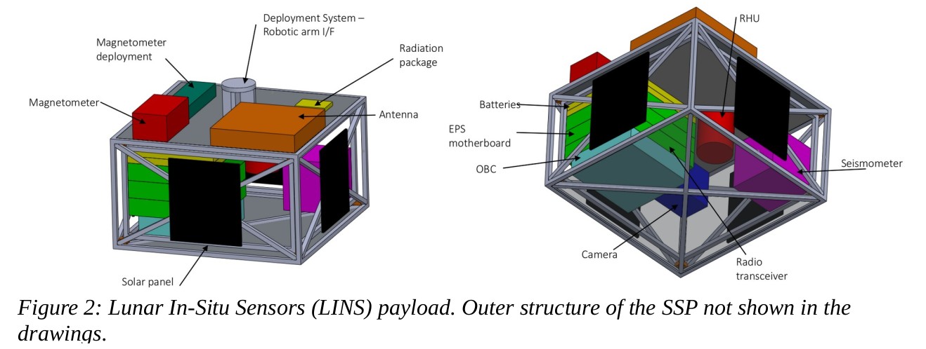
Moon SSP sensors:
LINS proposal is focused on two principal science objectives: understanding the structure and composition of the lunar interior and the characterization of the lunar surface environment in view of human exploration and resource extraction. The placement of a network of short period seismic stations will allow determining the thickness of the lunar crust (upper and lower) and its lateral variability. Due to smaller size the LINS has fever scientific sensors and many are common with the MINS packages. Magnetometer selected for LINS is based on the triaxial magnetometer developed by INTA for MetNet Mars mission. The sensor will require some modifications and adaptation of the ejection mechanism as well as temperature qualification for Lunar conditions.
Shared sensors:
The cameras of both MINS and LINS are based on the Athermalized Panchromatic Imaging System (APIS) low-resolution refractive camera used by INTA as a CubeSat payload which flew on-board the OPTOS satellite. It is based on a 1.3 MP CMOS image sensor from Cypress Semiconductor Corporation but the optics will be redesigned taking into account the applicable requirements for each mission.
Miniature wind sensors (Mars) and thermoprobes are based on the same sensor structure developed by UPC. The new type of sensor is a spherical shell divided into four sectors. To sense temperature and provide heating power, a customized 3 x 3 mm silicon die, including a platinum resistor, is attached to the inner side of each sector. In MINS the wind sensors are located in the deployable mast and the soil sensor is in a compartment below the surface in contact with the regolith. For LINS a dedicated deployment mechanism must be developed for the soil probe. The wind sensors and soil probes are currently in TRL 6.
The short period seismometer is based on a miniature MEMS resonator by Imperial College, previously used in InSight[8]. For LINS a variant of the sensor, called the Silicon Seismic Package, (SSP)[9] is proposed.
The impact accelerometer of MINS will be a new development. To miniaturise the accelerometer, a commercial part from PCB Piezotronics has been selected as the basis of the sensor and the complete sensor assembly will be developed and qualified by INTA. Lunar SSP also includes an accelerometer which is used to determine the attitude of LINS. It is based on an Analog Devices component ADXL327BCPZ, already qualified by INTA for Mars, but LINS missions requires even larger temperature range so additional qualification is foreseen.
The radiation monitors included in both missions are based in the Metal-Oxide-Semiconductor Field-Effect-Transistor (MOSFET) dosimeters. Proposed provider of MOSFET dosimeters is Tyndall National Institute.
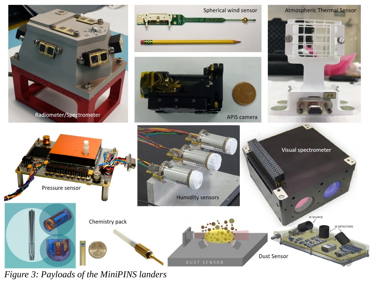
Project status:
The MiniPINS study, consisting of project phases A and B1, is nearly completed and a final review was held in autumn 2021. As a follow-up, the European Space Agency is facilitating an industrial development of European inflatable deceleration system.
How to cite: Hieta, M., Genzer, M., Haukka, H., Kestilä, A., Arruego Rodríguez, I., Apéstigue Palacio, V., Reina Aranda, M., Gonzalo Melchor, A., Martínez Oter, J., González-Guerrero Bartolomé, M., Ortega, C., Camañes, C., Dominguez-Pumar, M., Espejo Meana, S., Guerrero, H., and Rodríguez-Manfredi, J. A.: State-of-the-art miniaturised science instruments of the MiniPINS landers, Europlanet Science Congress 2022, Granada, Spain, 18–23 Sep 2022, EPSC2022-820, https://doi.org/10.5194/epsc2022-820, 2022.
- Introduction
In this work, we present the calibration of the NEWTON magnetic susceptometer for in-situ determination of the magnetic susceptibility of planetary surface rocks and regoliths. The susceptometer is based on inductive methods, and its operation does not require of sample preparation or manipulation. Current prototype has demonstrated capabilities for the determination of the complex magnetic susceptibility, i.e. real and imaginary component of the susceptibility [1, 2]. We propose the NEWTON susceptometer for the determination of the complex magnetic susceptibility, to provide valuable information about the regolith and surface rocks in rocky bodies of the solar system, to be used as a selection criterion of rocks for sample return missions or for the in-situ scientific studies of the magnetic properties during planetary missions.
- Calibration of the susceptometer
Due to the design of the instrument and the nature of the available magnetic susceptibility patterns [3], there are not available susceptibility calibration samples traceable to primary patterns with characteristics compatible with this device. The calibration procedure comprises a comparative methodology, consisting in two steps: the manufacture of magnetic susceptibility patterns, to serve as calibration samples of the real and imaginary parts separately for the NEWTON susceptometer; and the comparison of the results from the prototype with those from reference equipment.
The manufactured samples for the calibration of the real component of the magnetic susceptibility were made of ferrite powder diluted in a non-magnetic epoxy resin. Four samples of different mass content in ferrite powder were made, with the following distribution: a sample with 10% (weight %), a sample with 1%, a sample with 0,1% and a sample with 0,03% in ferrite powder. The homogeneity of the distribution of the ferrite powder within the samples was verified with X-ray images.
The imaginary susceptibility calibration samples were constructed using different techniques and comparing the results with other reference equipment. The sample used for calibration is made of 2.5mm diameter steel spheres (rolling bearing balls) distributed in a cubic lattice in a resin matrix providing both isotropic real and imaginary magnetic susceptibility values.
- Environmental testing
The most critical parts of the instrument have been submitted to qualification tests: vibration, thermal-vacuum and outgassing tests, applying the same requirements and test levels of those for the landing Mars mission, Exomars 2022, to demonstrate the capability of the instrument to withstand the interplanetary missions and space conditions.
- Application of the NEWTON susceptometer
The characterization of the complex magnetic susceptibility of rocks is an unexplored tool to constrain the composition, structure and geological history of rocks in surface planetary exploration [4]. The instrument is designed to measure a dynamic range of the real susceptibility from χ’ = 10-4 S.I. to χ’ = 101 S.I. for the real susceptibility, representative values for the rocks of the Earth, Moon and Mars [5, 6, 7]. The imaginary susceptibility measurement procedure has a resolution in the order of χ” = 10-6.
The sensor is suitable to be placed on board rovers, or to be used as a portable device during field campaigns and by astronauts in manned space missions. This sensor provides a great advantage compared to available commercial susceptometers, given that it does not require sample preparation, but only a minimum sample size (~50 x 20 x 20 mm). The current state of the susceptometer prototype consist of a portable device divided in two boxes: the Sensor Box (SB), containing the sensor core; and the Electronics Box (EV) containing the support electronics for the operation of the instrument (Figure 1).
The application of susceptibility measurements during space missions have a potential impact in the surface regolith and rocks characterization. The analysis of the samples from the Apollo missions [4], the characteristics of the Martian magnetic field [5], works in stony meteorites [6], Earth impact areas [7] and Earth analogues [8] highlight the enhancement of the scientific research that in situ magnetic field and magnetic susceptibility measurements provide to the Lunar and Martian exploration.
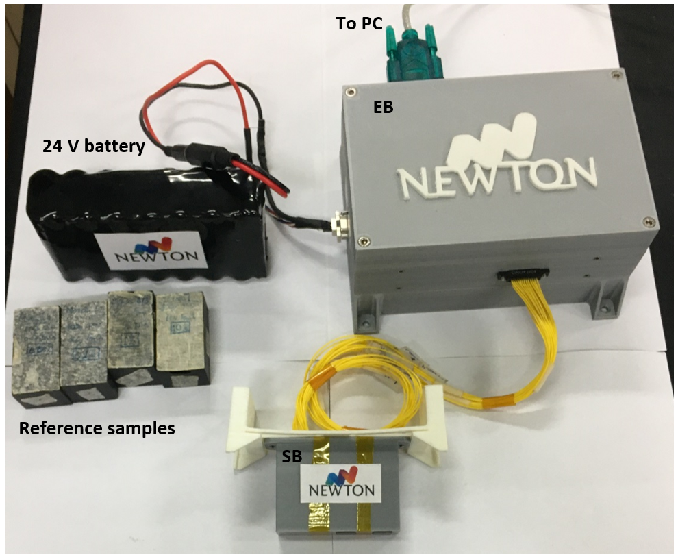
Figure 1. Image of the setup of the NEWTON instrument for in situ measurements during field campaigns, including reference samples for calibration.
Acknowledgement
This work has been funded by the Spanish Programme for Research, Development and Innovation under the grants of references ESP2017-88930-R and PID2020-119208RB-I00: MagAres and MINOTAUR, respectively, as well as the European Union Project NEWTON, of grant agreement 730041.
References
[1] J.L. Mesa et al. Feb. 2022. Submitted to IEEE Trans Instrum Meas.
[2] M. Díaz Michelena et al. 2017, Sensor Actuat A-Phys, vol. 263, pp. 471-479
[3] https://www.nist.gov/mml/materials-science-and-engineering-division/magnetic-moment-and-susceptibility-standard-reference. NIST. Retrieved May 4, 2022.
[4] M.S. Bentley et al. 2009, Planet Space Sci, vol. 57 (12), pp. 1491-1499.
[5] P. Rochette et al. 2006, Astrobiology, vol 6(3), pp. 423-36.
[6] P. Rochette 2010, Earth Planet. Sci. Lett., vol. 292, pp. 383–391.
[7] A. Collareta 2016, Meteorit Planet Sci, vol. 51 (2), pp. 351–371
[8] J. Pati, etl al 2016, Curr Sci India, vol. 111 (3), pp. 535-542.
How to cite: Mesa Uña, J. L., Díaz Michelena, M., and Aroca Hernández-Ros, C.: Calibration of NEWTON Susceptometer for fast and in-situ determination of the complex magnetic susceptibility., Europlanet Science Congress 2022, Granada, Spain, 18–23 Sep 2022, EPSC2022-864, https://doi.org/10.5194/epsc2022-864, 2022.
Introduction: The dust ejected by cometary nuclei encodes valuable information on the formation and evolution of the early Solar System. Several short-period comets have already been studied in situ[1], but their pristine condition was modified by multiple perihelion passages. Dynamically new comets (DNCs) remain pristine bodies since they never visited the inner Solar System, stationing more than 2000A.U. far away from the Sun in the Oort cloud.
Comet Interceptor (CI) is the first F-class space mission selected by the European Space Agency to study a DNC or an interstellar object entering the inner Solar System for the first time[2]. The Dust Impact Sensor and Counter (DISC) is an instrument included in the Dust Field and Plasma (DFP) suite, part of the CI payload, dedicated to characterizing the dust encountered by the spacecraft (S/C) during its flyby in the coma of the target DNC. DISC will measure hypervelocity impacts (HVIs), in the range 10–70km/s, with cometary dust particles of 1–400μm diameter. It aims to characterize the mass distribution of dust particles in the range 10-15–10-8kg, and retrieve information on dust structural properties from impacts duration[3].
DISC design: DISC is a 121×115.5×46mm3 aluminum box containing both the detection system and the electronics (Fig.1). The former consists in a 100×100×0.5mm3 aluminum plate with three piezoelectric traducers (PZTs) at its corners. HVIs induce shockwaves in the sensing plate. Far from the impacted area, such waves become acoustic Lamb waves that propagate up to the PZTs, which start to vibrate at their resonant frequency. A couple of electronic boards at the bottom of the unit allows to retrieve the particles momentum and kinetic energy from PZTs vibration signal.
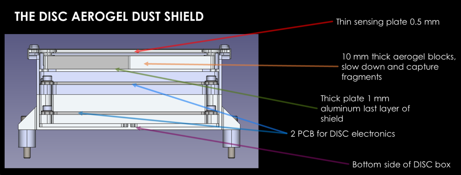 Fig.1: DISC sensing element and dust shield design.
DISC detection system is derived from the GIADA Impact Sensor measurement subsystem, that was designed to measure impacts of slow particles[4]. During CI flyby, some hypervelocity dust particles might perforate DISC outer sensing diaphragm and represent a serious hazard for the instrumentation. A dedicated mechanical element preliminarily designed as made of four 1cm-thick aerogel blocks and a 1mm-thick aluminum frame was integrated into DISC design to shield the entire S/C from such dangerous impacts.
Two key aspects need to be verified to ensure that the instrument is suitable for CI aims:
- DISC capability to survive the expected coma dust environment;
- DISC capability to measure the momentum/energy of impacting particles in the aforementioned size and mass ranges.
Dust shield assessment: We verified DISC dust shield performance using a two-stage Light-Gas Gun (LGG) (Open University, Milton Keynes) to shoot mm-sized particles of various materials at speeds around 5km/s[5,6]. This facility allowed to test the instrument resistance to momenta in the range 10-2–10-1kg·m/s and to energies of the order of 102J. The dust shield showed good resistance up to energies of about 200J, released by a 3mm nylon bead at 5.5km/s. DISC resistance to higher-energy particles can be improved by increasing the aerogel thickness, without any further modifications to the general design.
These experiments proved that DISC is compatible with the foreseen coma dust environment. Integrating a thicker aerogel layer in the design will reduce the risk of failure due to higher-energy particles to low enough values even for the S/C more exposed to the dust flux. The S/C beneath DISC unit is further protected by DISC lower layers.
DISC performance: DISC will measure momenta in the range 10-11–10-3kg·m/s[7]. The LGG facility allows to reach high momentum values by shooting heavy particles, but their collision dynamics is very different from what expected for cometary dust. A different strategy to simulate the foreseen impact momentum range is needed.
A Van der Graaf (VdG) gun can shoot μm-sized dust particles up to 20km/s, reproducing momenta of 10-9–10-7kg·m/s[8].
The tested impact parameters range can be extended by simulating HVIs effects with a high-power pulsed laser beam. Laser intensity, beam dimension, and pulse duration can be regulated to respectively match impact pressure, section, and shock duration of the corresponding particle[9]. Laser intensities of 109–1010W/cm2 can generate surface pressures from kbar to Mbar, typical of cometary dust particles colliding at 3–6km/s. Using our Nd:YAG laser (λ=1064nm), which emits τ=6ns pulses with pulse energy of Epulse=1.2J, we can cover a momentum range of 10-10–10-5kg·m/s. Since laser simulated and VdG real impacts share part of the released momentum range, laser shots can be calibrated and their representativity verified with real collisions.
The energy range expected for dust impacts measured during CI flyby is 10-7–102J. Laser simulated impacts cannot reach the higher energy values. However, the energy/pulse duration range is pretty vast and with some attenuators and pulse reducers the central/left part of the parameters space (around mJ energy and ns pulse time) could be reasonably covered.
Fig.2. shows the optical setup: a polarizer attenuator splits the beam and allows to regulate its power; a couple of mirrors prevents backwards reflections to get to the laser output aperture; a beam expander enlarges the beam, which enters a vacuum chamber and is focused by a plano-convex lens on the DISC breadboard mounted on a 3-axis translational stage. The vacuum chamber is fundamental to prevent plasma generation in air around the focus.
 Fig.2: Optical setup for high-power pulsed laser simulated HVIs.
By properly tuning the laser parameters, this strategy allows to achieve representative simulations of cometary dust HVIs. In addition to assess DISC performances, simulating the same impact many times provides large statistics to calibrate DISC detection system and momentum/kinetic energy retrieval methodology with great accuracy.
References: [1] Keller H. U. and Kührt E. (2020) Space Sci. Rev., 216(1), 1–26. [2] Snodgrass C. and Jones G. H. (2019) Nat. Commun., 10(1), 1–4. [3] Della Corte V. et al. (2021) LPSC LII, Abstract #2332. [4] Esposito F. et al. (2002) Adv. Space Res., 29(8), 1159–1163. [5] McDonnell J. A. M. (2006) Int. J. Impact Eng., 33(1–12), 410–418. [6] Hibbert R. et al. (2017) Procedia Eng., 204, 208–214. [7] Di Paolo F. et al. (2021) LPSC LII, Abstract #1238. [8] Friichtenicht J. F. (1962) Rev. Sci. Instrum., 33(2), 209–212. [9] Pirri A. N. (1977) Phys. Fluids, 20(2), 221–228.
How to cite: Ferretti, S., Della Corte, V., Piccirillo, A. M., Rothkaehl, H., Sylvest, M., Patel, M., Ertel, H., Millinger, M., Bertini, I., Fiscale, S., Longobardo, A., Inno, L., Rotundi, A., Ammannito, E., and Sindoni, G.: Analysis of dust shield and detection system response to hypervelocity impacts for Comet Interceptor Dust Impact Sensor and Counter, Europlanet Science Congress 2022, Granada, Spain, 18–23 Sep 2022, EPSC2022-1163, https://doi.org/10.5194/epsc2022-1163, 2022.
MITM8 | Synergistic exploitation of small body missions in the 2020s
(385186) 1994 AW1 was the first known asteroid with a satellite, discovered in 1994 using photometric lightcurve [1], the most successful technique used for this purpose. After that, more than 450 asteroids with satellites were discovered in the Solar System [2], almost 80% of them with orbits up to Jupiter, using many other observation techniques such as radar, and direct imaging from the ground and space. Recently in 2021, it was the first time that a stellar occultation provided the discovery of a companion asteroid by two independent events [3]. But still, a whole range of separation and size ratios is out of reach, where asteroids are too faint for high-resolution imaging, too far for radar, or do not provide a good signature in photometry. In that range, the use of highly accurate astrometry could be promising. In binary star research, companions are revealed by astrometry when the motion of a star around the common barycentre is measured (wobbling). The same approach becomes possible for asteroids, for the first time thanks to Gaia astrometry. As predicted way before the launch of the Gaia satellite[4], the high accuracy astrometric data could be used to find binary asteroids currently out of reach of detection. The Gaia mission provided to the scientific community astrometric solutions at an unprecedented precision [5]. Data Release 3 (DR3) provides new data for more than 150.000 asteroids, 10 times more than in Gaia DR2. Hence, using a large number of bodies in DR3 data with even better precision than in previous releases, we aim to search for astrometric asteroid binaries. Our approach starts by averaging the residuals to orbital fits over each transit in the focal plane. We select the asteroids with at least 10 values of residuals that are consecutive in time or anyway spanning a limited time range. This selection results in a sample of a bit more than 30000 objects. Then, using a Generalized Lomb-Scargle periodogram (see [6] and references therein), we run a period search on every sequence in order to find a signal that would represent the period and amplitude of the system's wobbling. The result is a map of the frequency power that indicates the goodness of data fitting. Since this technique always finds periodic fluctuations that could be spurious because of residual noise, we perform some statistical tests to determine the probability of fake detection and the relevance of the signal found. The first procedure is to run 10000 Monte Carlo simulations on white noise using the same time-sampling as the real data. The resulting p-value shows us how likely it is to obtain a peak as large as the largest peak found in the data if there was only noise in the data. The bodies that have a p-value smaller than 5% pass through the second calibration test. Again we perform 2000 MC simulations while adding white noise to the real data and checking how it affects the distribution of frequencies obtained from the GLS periodogram. If at least 10% of the distribution lies around the best frequency found for the real data, then we select this body. This procedure tells us the quality and confidence of the signal found, i.e., how easy it is to detect and how much we can trust that there is a signal in the data. After the period search and statistical relevance tests, we obtain over 3300 candidates as possible binary asteroids. The last step is to check if the wobbling found is physically consistent. Hence we calculate the estimated range of density, separation and mass ratio for the binary candidates. We consider 7 g/cm3 as a maximum threshold for an acceptable maximum density. In the end, we obtained almost 250 asteroid binary candidates that survived the 3-stage selection. We still can't guarantee that the periods found with such favourable conditions are caused by a companion satellite, but we show that there are some interesting pieces of evidence to support such a hypothesis. Further verification is required, both by statistical methods and observations, to validate our findings.
References
[1] Pravec, P. & Hahn, G. 1997, Icarus, 127, 431
[2] Johnston, Wm. Robert. "Asteroids with Satellites Database" May 16, 2022. Johnston's Archive
[3] Gault D., Nosworthy P., Nolthenius R., Bender K., Herald D., 2022, MPBu, 49, 3
[4] Tanga, P., Hestroffer, D., Delbò, M., et al. 2008, Planetary and Space Science, 56, 1812
[5] Gaia Collaboration, Spoto, F., Tanga, P., et al. 2018b, Astronomy and Astrophysics, 616, A13
[6] VanderPlas, J. 2018, ApJS, 236, 16
[7] Hestroffer, D., Dell’Oro, A., Cellino, A., & Tanga, P. 2010, in Lecture Notes in Physics, Berlin Springer Verlag, Vol. 790, 251–340
Acknowledgements
This work presents results from the European Space Agency (ESA) space mission Gaia. Gaia data are being processed by the Gaia Data Processing and Analysis Consortium (DPAC). Funding for the DPAC is provided by national institutions, in particular the institutions participating in the Gaia MultiLateral Agreement (MLA). The Gaia mission website is https://www.cosmos.esa.int/gaia. The Gaia archive website is https://archives.esac.esa.int/gaia.
This study was financed in part by the Coordenação de Aperfeiçoamento de Pessoal de Nível Superior – Brasil (CAPES) – Finance Code 001, also by CAPES-PRINT Process 88887.570251/2020-00, by the French Programme National de Planetologie, and by the BQR program of Observatoire de la Côte d'Azur.
How to cite: Liberato, L., Tanga, P., Mary, D., and Spoto, F.: Satellite Search in Gaia DR3 astrometry, Europlanet Science Congress 2022, Granada, Spain, 18–23 Sep 2022, EPSC2022-630, https://doi.org/10.5194/epsc2022-630, 2022.
MITM9 | Advances in Mass Spectrometry for Spaceflight Applications
The MAss Spectrometer for Planetary EXploration (MASPEX) instrument is a multi-bounce time-of-flight mass spectrometer designed for high mass resolution and sensitivity. MASPEX-Europa will launch as part of the Europa Clipper mission payload in October 2024 to characterize the composition of major, minor, and trace neutral gases in Europa’s exosphere and potential plumes. The instrument has been designed to optimize measurement of complex natural environments with:
- Variable mass resolution to support compositional reconnaissance with simultaneous measurement of ions from 2 u to 500 u at separation of unit masses, as well as focused analysis with mass resolution capable of separating CHN- and CHO-bearing organics over a more narrow mass range
- Nearly 100% duty cycle via storage of ions in the source between extraction pulses
- Exact mass identification via measurement in flight of the FC-43 calibrant gas
- Measurement of trace compounds via enhancement of abundance with the cryocooler
- Automated switching triggered in flight between “regular” and “ice grain” measurement parameters for optimization of data collection
These adaptations make MASPEX especially well-suited for data collection in a dynamic environment where measurement speed is important. The capability to provide both general and highly specific data on the composition of volatile and organic mixtures makes MASPEX very powerful to quantify habitability via geochemical indicators, and to search for the first, perhaps tentative signs of life beyond Earth via measurements of agnostic biosignatures such as isotopic ratios.
In this presentation, we will provide results from the final calibration and performance characterization of the MASPEX-Europa flight model instrument completed in summer 2022. We will also present the science that will be enabled for Europa Clipper, and how new scientific and technical innovations will allow MASPEX to open more windows into planetary evolution, cosmochemistry, and astrobiology for future missions.
How to cite: Miller, K., Miller, G., Waite, H., Brockwell, T., Franke, K., Hoeper, P., Perryman, R., Glein, C., and Burch, J. and the MASPEX science and engineering teams: Onwards to Europa: Results from the final ground calibration of the MASPEX-Europa flight instrument, Europlanet Science Congress 2022, Granada, Spain, 18–23 Sep 2022, EPSC2022-705, https://doi.org/10.5194/epsc2022-705, 2022.
Introduction
The organic molecular diversity present in extraterrestrial bodies such as asteroids and comets is of great interest for understanding the origin of life. However, the onboard analytical techniques are essentially low resolution mass spectrometry which, in view of the molecular diversity, quickly present limits both in the identification of compounds and in the comprehensive understanding of the composition of this type of sample. It is therefore interesting to question the interest to develop high resolution mass spectrometry for future space missions. In this context, the cosmorbitrap consortium is developing the spatialization of the Orbitrap. In addition, to optimize the identification of compounds within the samples to be analyzed, the coupling of such a technology to a gas chromatograph would also provide a gain in resolution and thus improve the characterization of the targeted samples.
In this perspective, a first development was carried out for a targeted analysis focusing on the detection of amino acids within analogues of soluble organic matter of meteorites [1] [2]. These molecules are particularly interesting because they have been detected in some meteorites and can be markers of the chemical evolution of the studied object [3]. Moreover, they could have played an important role in the homochirality observed on Earth [4]. In a second step, the same samples were analyzed by pyrolysis and thermal desorption, two sampling techniques usually used for in situ GC-MS analyses.
Materials and methods
Samples were analyzed on a GC-FT-Orbitrap-MS (Trace 1310 gas chromatograph with a Q-Exactive OrbitrapTM MS analyzer from Thermo Fisher Scientific).
Targeted amino acid analyses were performed on a chiral column: Chirasil-L-Val (Agilent). Pyrolysis and thermodesorption were performed on an RXi-5MS column (Restek). Evolved gas analyses (EGA) required the use of an inert column with an isothermal oven temperature.
For the analysis of the amino acid solution within the soluble organic meteorite analogues in GC-Orbitrap, a preliminary derivatization step was performed according to the method of Meinert and Meierhenrich [5].
The analogues were formed using the MICMOC device as described [6].
Preliminary results and conclusions
The optimization of the parameters and the realization of the calibration provide values of limit of detection and quantification as well as the sensitivity. A sensitivity in the order of 10-6 M is obtained .
Once optimized, the analysis of the amino acids within the analogues allows to observe about ten amino acids in full scan (see Fig. 1). By mass extractions about fifteen amino acids are identified. The use of GC-orbitrap for the targeted analysis of amino acids presents performances equivalent to those observed by GCxCG-TOFMS on the same samples, with higher detection and quantification limits.

Fig. 1. Full scan GC-orbitrap chromatogram of a derivatized residue for amino acids detection. Aminoacids are numbered as following : 1, Sarcosine; 2, D-Alanine; 3 : L-Alanine; 4, Glycine; 5, β-Alanine; 6, Methionine; 7, 2,3-DAPA.
In a second step, an EGA analysis of the same analogue was performed by thermodesorption (Fig. 2). The direct injection allows the rapid identification of molecules such as hexamethyletetramine (HMT) thanks to the high resolution of the mass spectrometer allowing to obtain the raw formula. Moreover, due to the possibility of obtaining these raw formulas a polymer of CHN composition is observed. To confirm these first results, an analysis via GC of the same sample allowed to confirm these first observations.
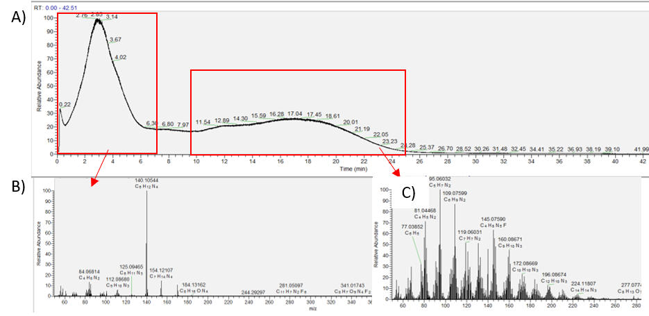
Fig. 2. EGA analysis of the non-derivatized residue. A) Chromatogram of the thermodesorption analysis. B) HMT derivatives. C) Mass spectrum of a CHN polymer.
These first data show that very high resolution mass spectrometry is an essential tool for the characterization of samples with a large molecular diversity. Coupled or not with a gas chromatograph, it allows to obtain raw formulas improving the identification of compounds in targeted analysis, and allowing to obtain information on the molecular content of a sample in direct analysis. Very high resolution mass spectrometry coupled or not to a GC is thus a promising technology for the future in situ analysis of interplanetary objects such as asteroids and comets.
Reference
[1] Muñoz Caro, G., Meierhenrich, U., Schutte, W. et al. Amino acids from ultraviolet irradiation of interstellar ice analogues. Nature, 2002, 416, 403–406
[2] G. Danger, F.-R. Orthous-Daunay, P. de Marcellus, P. Modica, V. Vuitton, F. Duvernay, L. Flandinet, L. Le Sergeant d’Hendecourt, R. Thissen, T. Chiavassa, Characterization of laboratory analogs of interstellar/cometary organic residues using very high resolution mass spectrometry, Geochimica et Cosmochimica Acta, 2013, Volume 118, 184-201
[3] Martins, Z., Modica, P., Zanda, B. and d'Hendecourt, L.L.S., The amino acid and hydrocarbon contents of the Paris meteorite: Insights into the most primitive CM chondrite. Meteorit Planet Sci, 2015, 50, 926-943.
[4] Iuliia Myrgorodska, Cornelia Meinert, Zita Martins, Louis le Sergeant d’Hendecourt, Uwe J. Meierhenrich. Quantitative enantioseparation of amino acids by comprehensive two-dimensional gas chromatography applied to non-terrestrial samples. Journal of Chromatography A, 2016, 1433, 131-136
[5] C. Meinert, U.J. Meierhenrich, Derivatization and multidimensional gas-chromatography resolution of a-alkyl and a-dialkyl amino acid enantiomers, ChemPlusChem, 2014, 79, 781-785
[6] L. d’Hendecourt and E. Dartois, Interstellar matrices: the chemical composition and evolution of interstellar ices as observed by ISO, Spectrochim. Acta A Mol. Biomol. Spectrosc., 2001, 57, 669–684
How to cite: Garcia, A., Meinert, C., Poinot, P., and Danger, G.: Orbitrap and GC-Orbitrap for in situ analyses: clues from laboratory experiments, Europlanet Science Congress 2022, Granada, Spain, 18–23 Sep 2022, EPSC2022-1075, https://doi.org/10.5194/epsc2022-1075, 2022.
Ocean worlds in our Solar System have captivated the attention of scientists due to the presence of liquid water that could make it possible for these worlds to harbor life. Because all life on Earth is built from a selected set of organic molecules, clear patterns appear in the relative distribution of organics when a sample has a biotic origin. A powerful approach in the search for life involves seeking for such chemical patterns. The liquid-based separation technique of capillary electrophoresis (CE) holds unique promise for this task. CE is a high-resolution separation technique for molecules in solution that allows the analysis of a broad range of compounds using a relatively simple instrumental set up. CE separations occur within small diameter glass capillaries (25-100 mm I.D.) filled with a background electrolyte. CE is an ideal candidate for in situ planetary missions, especially to areas where aqueous analysis is required.
Although CE can be coupled to multiple detectors, mass spectrometry (MS) is particularly attractive for planetary exploration because it adds another separation dimension based on mass-to-charge (m/z) ratios. Although there are multiple ionization techniques to couple CE to MS, the most common one is electrospray ionization (ESI). With ESI, the compounds that are separated by CE can be efficiently transferred from the liquid phase into the gas-phase. The coupling of CE and MS allows detailed characterization of biomolecules, and more importantly the identification of unknowns in complex mixtures. We have recently reported on the development of a CE instrument that can be coupled to multiple detection systems, including MS 1. Other detectors include laser-induced fluorescence for sensitive analysis of amino acids and contactless conductivity detection for analysis of inorganic ions and organic acids. This system is under development for biosignature detection as part of the Europan Molecular Indicators of Life Instrument (EMILI)2 and the Ocean Worlds Life Surveyor (OWLS).
Based on the major constituents potentially expected in the oceans of Enceladus and Europa, we used NaCl and MgSO4 salts to evaluate the effect of Na+, Mg2+, Cl-, and SO42- on the detection of a wide range of organics by CE-MS using a sheathless interface 3. We have selected a mixture of amino acids, peptides, nucleosides, and nucleobases for this study, all of which are building blocks of the main polymers of terrestrial biology and are associated with at least one of the rungs of the Ladder of Life. We demonstrate CE-MS limits of detection for these organics ranging from 0.05 to 1 mM (8 to 8 ppb), in the absence of salts. More importantly, organics in the low mM range (1 to 50 mM) are detected by CE-MS in the presence of 3 M NaCl without desalting, preconcentration or derivatization 3. The applicability of CE-MS for analysis of challenging natural samples was demonstrated by analysis of samples from Mono Lake. Multiple organics were detected in the sample despite the presence of a salt front. These results demonstrate the potential of CE-MS for in situ organic analysis on future missions to ocean worlds.
How to cite: Mora, M., Kok, M., Noell, A., and Willis, P.: Capillary Electrophoresis Coupled to Mass Spectrometry for the Detection of Organics in High Salinity Samples Relevant to Ocean Worlds, Europlanet Science Congress 2022, Granada, Spain, 18–23 Sep 2022, EPSC2022-1194, https://doi.org/10.5194/epsc2022-1194, 2022.
In 2005, a new type of mass spectrometer was commercialised for the first time, the Thermo Fisher Scientific OrbitrapTM. Using a Quadro-Logarithmic Electrostatic Ion Trap technology, Orbitrap mass spectrometers are able to reach ultra-high mass resolution1. For a decade, the Laboratoire de Physique et Chimie de l’Environnement et de l’Espace (LPC2E) is developing a spatialised version of the Orbitrap, the CosmOrbitrap2, to bring this high resolution in space exploration. The CosmOrbitrap is intended to be the mass analyser and acquisition system of laser ablation mass spectrometers aiming for planetary bodies like Europa or the Moon3,4.
In this context, OLYMPIA - Orbitrap anaLYser MultiPle IonisAtion – has been develop to be used as a new laboratory test bench, and is adaptable to different ionisation methods. After a successful study of planetary atmosphere analogues using Electron Ionisation (EI)5, we now coupled OLYMPIA with the Laser Induced Liquid Beam Ion Desorption technique to analyse liquid water samples. For example, LILBID is able to accurately reproduce hypervelocity impact ionisation icy grains mass spectra6, such as those recorded by the Comic Dust Analyser7 (CDA) onboard Cassini in the vicinity of Saturn’s icy moon Enceladus. The LILBID setup is usually coupled with a Time-of-Flight (TOF) mass spectrometer, with a mass resolution of ~800 m/Δm. By coupling the LILBID technique to OLYMPIA and its Orbitrap analyser, we are now able to record hypervelocity icy grains analogue mass spectra with ultra-high mass resolution. The setup is currently able to measure H2O+ and H3O+ ions with a mass resolution of around 150.000 m/Δm (FWHM), with the spectral appearance matching mass spectra of icy grains impact ionisation in an impact velocity range of 15 to 20km/s. Future work aims to simulate lower impact velocities below 15 km/s as they are typically expected for flyby or orbiter missions.
Those results will be implemented in the LILBID database8, and will be useful for the calibration and future data interpretation of the SUrface Dust Analyser (SUDA) mass spectrometer9, which will be onboard NASA’s Europa Clipper mission10 to characterize the habitability of Jupiter’s icy moon Europa.
References
1. Makarov, A. Electrostatic Axially Harmonic Orbital Trapping: A High-Performance Technique of Mass Analysis. Anal. Chem. 72, 1156–1162 (2000).
2. Briois, C. et al. Orbitrap mass analyser for in situ characterisation of planetary environments: Performance evaluation of a laboratory prototype. Planet. Space Sci. 131, 33–45 (2016).
3. Arevalo, R. et al. An Orbitrap-based laser desorption/ablation mass spectrometer designed for spaceflight. Rapid Commun. Mass Spectrom. 32, 1875–1886 (2018).
4. L. Willhite et al. CORALS: A Laser Desorption/Ablation Orbitrap Mass Spectrometer for In Situ Exploration of Europa, 2021 IEEE Aerospace Conference (50100), 2021, pp. 1-13, doi: 10.1109/AERO50100.2021.9438221.
5. Zymak, I. et al. OLYMPIA - a compact laboratory Orbitrap-based high-resolution mass spectrometer laboratory set-up: Performance studies for gas composition measurement in analogues of planetary environments. https://meetingorganizer.copernicus.org/EGU21/EGU21-8424.html (2021) doi:10.5194/egusphere-egu21-8424.
6. Klenner, F. et al. Analogue spectra for impact ionization mass spectra of water ice grains obtained at different impact speeds in space. Rapid Commun. Mass Spectrom. 33, 1751–1760 (2019).
7. Srama, R. et al. The Cassini cosmic dust analyser. Space Sci. Rev. Volume 114, 465–518 (2004).
8. Klenner, F. et al. Developing a Laser Induced Liquid Beam Ion Desorption Spectral Database as Reference for Spaceborne Mass Spectrometers. Earth and Space Science Under Review (2022).
9. Kempf, S. et al. SUDA: A Dust Mass Spectrometer for Compositional Surface Mapping for a Mission to Europa. European Planetary Science Congress 2014, EPSC2014-229.
10. Howell, S. M. & Pappalardo, R. T. NASA’s Europa Clipper—a mission to a potentially habitable ocean world. Nat. Commun. 11, 1311 (2020).
How to cite: Sanderink, A., Klenner, F., Zabka, J., Postberg, F., Lebreton, J.-P., Zymak, I., Bertrand, G., Abel, B., Charvat, A., Cherville, B., Thirkell, L., and Briois, C.: OLYMPIA-LILBID: High Resolution Mass Spectrometry for the Calibration of Spaceborne Hypervelocity Ice Grain Detector, Europlanet Science Congress 2022, Granada, Spain, 18–23 Sep 2022, EPSC2022-1252, https://doi.org/10.5194/epsc2022-1252, 2022.
How Life has emerged on Earth? Can we find signs of Life on other celestial bodies in the Solar System? Are they harboring liquid water and complex-enough organic matter to initiate Life? What actually complex-enough organic matter means? Among other scientific questions, those related to astrobiology drive the future space missions for decades to come. The search for organic compounds in the Solar System, such as bio- and prebiotic molecules, has been defined as one of the highest priority by the Space Agencies [1, 2].
Significant improvements of the analytical performances of the future instruments will increase our knowledge of targets of interest for the search of Life, present or past, such as comets, asteroids, icy moons or ocean worlds. New generation of High Resolution Mass Spectrometers (HRMS) is currently being developed in order to provide univocal identifications, study of isotopic abundances and determination of mixing ratios with high analytical performances [3-6], including very HRMS-CosmOrbitrap based under collaborative development with University of Maryland/NASA Goddard Space Flight Center. The CosmOrbitrap mass analyzer is mainly funded by CNES, the French space agency, and developed by a consortium of 6 laboratories (LPC2E, LATMOS, LISA, IPAG, IJC lab, J. Heyrovsky Institute of Physical Chemistry) [7].
Here we address the results of a repeatability study based on three organic compounds and obtained with the LAb-CosmOrbitrap (Laser Ablation CosmOrbitrap) equipped with a commercial laser ionization system at 266 nm and no C-trap system. Organics studied are nitrogenous and sulfurous compounds, HOBt (C6H5N3O+H) at m/z 136 and BBOT (C26H26N2O2S+H) at m/z 431; and a prebiotic compound, the well-known adenine (C5H5N5+H) at m/z 136.
Hundreds of mass spectra have been recorded to demonstrate the reproducible analytical performances of the laser-CosmOrbitrap set-up. Mass resolving power has been studied as a function of the acquisition time and the FFT length. Different kind of mass calibrations have been tried to show the effect on the mass accuracy (internal mass calibration on the species of interest and external mass calibration on the metallic sample-holder). Finally, preliminary results on isotopic abundances (13C/12C, 15N/14N and 34S/32S replacements) have been obtained.
This work provides key information for specifying the required performances of future HRMS space instruments.
Acknowledgement: We thank the Centre National des Etudes Spatiales (CNES), the French space agency, for their financial support.
References:
[1] National Academies (2022) Origins, Worlds and Life.
[2] ESA (2021) Voyage 2050
[3] Waite et al. (2019) Abstract Vol.13, EPSC-DPS2019-559-1
[4] Shimma et al. (2010) Anal. Chem. 82, 20, 8456-8463
[5] Willhite et al. (2021) IEEE Aerospace, 1 – 13
[6] Willhite et al. (2021) Annual Meeting of the Lunar Exploration Analysis Group, LPI Contribution No. 2635, id.5034
[7] Briois et al. (2016) PSS 131, 33 – 45
How to cite: Selliez, L., Briois, C., Carrasco, N., Thirkell, L., Gaubicher, B., Lebreton, J.-P., and Colin, F.: The potential of the LAb-CosmOrbitrap for future space studies in astrobiology, Europlanet Science Congress 2022, Granada, Spain, 18–23 Sep 2022, EPSC2022-1259, https://doi.org/10.5194/epsc2022-1259, 2022.
MITM11 | Tools and Data Analytics for Solar and Planetary Sciences
The European Space Agency’s Planetary Science Archive (PSA) is the home for all scientific data from ESA’s planetary missions. Adopting the NASA PDS standard (version 3 and 4) it is designed to make the data, meta-data and knowledge on how to use them available to the scientific community. As a multi-mission archive, the PSA supports (or will soon support) over ten missions and their associated instruments, with this number expected to grow significantly in the coming years.
The PSA has a long legacy of successfully preserving and distributing mission data to the community, and offers several services to fulfil this, including tabular, image-based and map-based interfaces, several APIs and traditional FTP. However, the entry barrier for new users is quite high, and moving forward there are new data access requirements coming from scientists wanting to perform more complex queries, run machine learning algorithms and so on. This presentation will describe the current infrastructure, recent updates and plans for the next few years which will try to address these changing needs.
In particular, the following key developments are foreseen:
- implementation of a new user interface, with a streamlined and more user-friendly design, which will also work well on mobile, and touchscreen displays,
- improvements to APIs to include more data (specifically instrument geometry), and to incorporate the new PDS API which will allow access to any meta-data in the data products, leveraging the full value of the effort put in by instrument teams and archive scientists to curate them,
- integration with ESA DataLabs, a project designed to “bring the code to the data” and allow data processing and analysis to be done in an interactive online environment hosted close to the data repository and allowing big data workflows without having to download the products,
- publication of data tutorials based on open-source tools and libraries, to give new users a “quick start guide” to using data from a given instrument, and
- a much higher frequency release cadence, responding to the needs of the scientific community in a timely manner.
Finally, community input is sought on other improvements which could be made, and which use cases are not fulfilled by the current infrastructure.
How to cite: Bentley, M., Breitfellner, M., Coia, D., Docasal, R., Heather, D., Grotheer, E., Lim, T., Merín, B., Oliveira, J., Osinde, J., Raga, F., Saiz, J., and Valles, R.: ESA’s Planetary Science Archive: current status and future plans, Europlanet Science Congress 2022, Granada, Spain, 18–23 Sep 2022, EPSC2022-111, https://doi.org/10.5194/epsc2022-111, 2022.
Introduction: The present abstract is intended to show the current ESA’s Planetary Science Archive (PSA) [1] in terms of architecture/infrastructure and the future interfaces and technologies which will be used in the next generation archive.
These improvements range from a new graphical user interface developed in Angular to a TAP+ (Table Access Protocol) service as a single access to the data, through a new way of releasing new versions of the PSA more frequently to the scientific community.
The PSA development team expects to release this new generation of the PSA this summer 2022.
PSA current architecture: The PSA architecture and the technologies involved in its development have only undergone incremental updates in the last 6 years, and are now seen as somewhat obsolete. The front-end has been implemented using the Vaadin framework, which was initially a good strategy, but over time became onerous to maintain (e.g., dealing with JavaScript libraries, wasting time in wrapping some required extensions in Java).
Also, from the back-end point of view, there are many interfaces/libraries to access the database (JDBC, PDAP, Data Distribution, etc) forcing us to double the effort when changing the API (see Figure 1: PSA current architecture)
In addition, the PSA release approach has not followed a truly Agile approach, taking too long in releasing operationally. This is mainly due to the fact there is no a fully CI/CD strategy to be executed in the environments, leading to very manual release process with manual interventions. Also there are additional problems such as the synchronisation of the repositories when releasing, which strongly depends on the IT department.
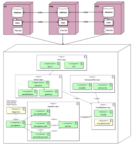
Figure 1: PSA current architecture
New interfaces, technologies and infrastructure at PSA: After one year and half of development, the PSA development team has been able to achieve several goals on the roadmap to a new archive. Mainly, we will rely on a new graphical user interface implemented under the Angular framework (see Figure 2: Future PSA Graphical User Interface). There have been various reasons to migrate to this new technology: Faster development for maps visualisation and 3D interfaces, alignment within the ESDC department in a common front-end framework and also, the discontinuation of Vaadin 8 from March 2022 on.
This future GUI will have a modern look and feel, with some relevant changes in line with the new ESA branding. Specially on the home view, where there are now card layouts to access the data from missions/instruments, targets and maps and a prototype traverse view for the ExoMars Rover mission, among other features. This new Angular framework has definitely sped the development up when modifying some JavaScript libraries, creating some end-to-end tests on top through Cypress, etc. This will also increase the performance on the client side consequently improving the user experience. In addition, this implementation is also mobile and tablet friendly/responsive.
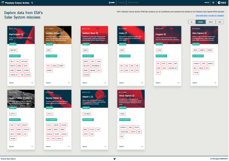
Figure 2: Future PSA Graphical User Interface
Also, the new PSA will count on a single access point to the data through TAP+ (even private data) to homogenise the access by offering a single API, instead of using different interfaces/protocols (JDBC, PDAP, etc.) to access the information.
In addition to these new interfaces, the PSA is making a huge effort to set up an infrastructure to support a faster deployment cycle in order to be more agile according to the scrum methodology. This implies integrating and deploying the software (after checking metrics in Sonar, passing the end-to-end tests, etc.) as nightly builds into a safe environment (pre-production) so that the Archive Scientists can test the latest features which, once approved, will go to the operational environment. This follows mostly a DEV-OPS infinite loop but having a middle environment (PRE) in which the scientists can safely test the features.
Conclusion: The current PSA development team along with the Science Lead and all of the Archive Scientists are working together to produce a new generation of the planetary archive, with these features:
- a more modern and responsive GUI based on a stable and well-known technology
- a single access route to the data with authentication and authorization for private products (TAP+)
- a new infrastructure of environments which allow a more efficient CI/CD so that the features can be validated earlier, allowing the PSA to offer releases in the operational environment more frequently.
References:
[1] Besse, S. et al. (2017) Planetary and Space Science, 10.1016/j.pss.2017.07.013, ESA's Planetary Science Archive: Preserve and present reliable scientific data sets.
Acknowledgments: The authors would like to thank everybody, especially the PSA development team, who have contributed to the development of the PSA in the recent years and the incoming new generation of the archive.
How to cite: Docasal, R., Felix-Redondo, F., Oliveira, J., Osinde, J., Raga, F., Saiz, J., Valles, R., Merin, B., Bentley, M., Coia, D., Grotheer, E., Heather, D., and Lim, T.: ESA’s Planetary Science Archive: present and future, Europlanet Science Congress 2022, Granada, Spain, 18–23 Sep 2022, EPSC2022-127, https://doi.org/10.5194/epsc2022-127, 2022.
The Mission Analysis and Payload Planning System (MAPPS) is a multi-mission software system developed during the last 20 years to support the science operations planning for the ESA solar system missions at the European Space Astronomy Centre (ESAC) near Madrid.
Developed initially only to visualise the coverage of MEX experiments onto the Martian surface. The tool has been evolved progressively to satisfy planning requirements for the different missions that have been launched in the last two decades: SMART-1, Venus Express, Rosetta, Mars Express, Exomars TGO, Bepi Colombo, Solar Orbiter, Juice and EnVision.
The planning requirements sometimes are specific to a mission and on other occasions they are contradicting. As an example, consider the power and thermal requirements of a mission like Bepi Colombo, very close to the sun, in contrast to those same requirements for a mission like Juice, very far away. The complexity of these requirement implies that the software needs to be very configurable and continuously adapting to the needs of each mission.
In recent years, there has been the need to extend even further the tool to support multi-body and constellation coordination capabilities.
In the case of Juice, the spacecraft will spend many months orbiting Jupiter and three of its Jovian moons. This has required a big effort to modify the existing features and observations in MAPPS that were initially developed for a central body to be able to cope with several bodies.
In the case of Mars, the arrival of new spacecrafts and rovers has broadened what can be done scientifically as well as opening the international collaboration among agencies. MAPPS has been extended to facilitate the collaboration with other Mars missions, in particular the new radio-science experiment between MEX-TGO [1], various communication tests between ESA and NASA orbiters, and the regular data relays in support of all surface assets, including the new Chinese Zhurong mission.
Here we present how MAPPS has contributed and supports the Science Ground Segment teams in ESA to achieve their goal of planning scientific operations in an efficient and optimised way, together with the new features implemented for the ever more demanding needs of the new scientific missions.
[1] Cardesin Moinelo, A. et al: First year of coordinated science observations by Mars Express and ExoMars 2016 Trace Gas Orbiter, ICARUS 353, 2021
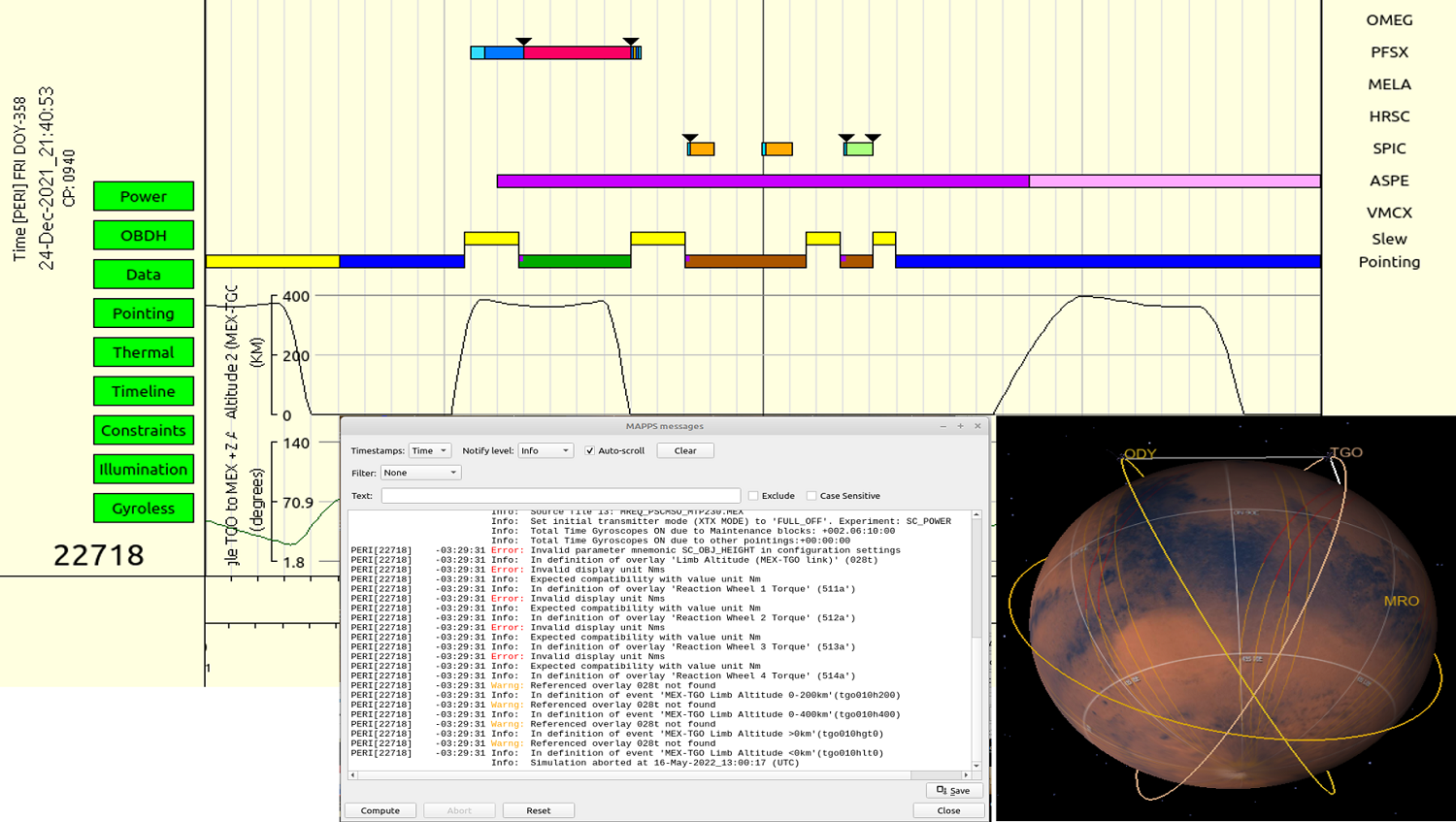
How to cite: Muñiz Solaz, C., Cardesin-Moinelo, A., Nespoli, F., Martin, P., Marin-Yaseli de la Parra, J., Merrit, D., Sierra, M., and Esquej, P. and the ESA Planetary Science Operations Centres: MAPPS as a multi-mission and multi-body Science Planning and Simulation Tool for ESA solar system missions, Europlanet Science Congress 2022, Granada, Spain, 18–23 Sep 2022, EPSC2022-294, https://doi.org/10.5194/epsc2022-294, 2022.
Introduction
The small bodies (also known as minor planets) in our solar system are usually discovered by telescopic surveys. The results of these observations are organised by the Minor Planet Center (MPC), which determines orbits from the astrometric observations of the surveys. As of May 15, 2022, the MPC has an orbit database of 1,193,635 minor planets. However, the MPC data do not tell us what a minor body actually is, as they not contain physical properties such as albedo, diameter, volume, shape, composition, mass, bulk density, period of rotation and direction in the sky of the axis of rotation. Asteroids have very diverse values of these physical properties, whose knowledge is important for scientific studies of our solar system and its origin, planetary formation and evolution, space exploration, and planetary defence.
The physical properties of small bodies are spread across many publications, several websites (e.g. the NASA planetary data service) and archives. Many compositionally diagnostic spectra are also presented in a series of publications, but their source files are not necessarily public. This poses a fundamental problem to our ability to massively exploit the physical properties of minor bodies. Moreover, the values of these physical parameters are extremely heterogeneous, obtained by several different groups, project teams and telescopic surveys, and even individual researchers, using different techniques. For example, thermal models are used to interpret observations in the mid-infrared (between 3.5 and 100 μm) from space and from the ground for the measurement of diameters and albedos. However, other techniques such as radar or the measurement of stellar occultation times provide measurements of diameters.
A centre of minor planets’ physical properties
The Minor Planet Physical Properties Catalogue, or MP3C for short, collects and organises in a single place and makes available to the community values of physical properties of asteroids and other small bodies of our solar system. The MP3C is designed for very heterogeneous and big amount data: as of March 2022 it contains 3,710,587 measured properties, all of which are fully referenced to their published sources. The MP3C offers two main interfaces to explore the data (Figs. 1 and 2), namely (i) a web portal (mp3c.oca.eu) that allows to perform extraction of physical properties values on the basis of a single or list of minor bodies identifiers (names, numbers), but also on ranges of physical and dynamical properties; (ii) a data server offering a Table Access Protocol (TAP), which is defined and compatible with the standards of the Virtual Observatory (VO). The data server is accessible at https://dachs.oca.eu. MP3C is registered as service of the Virtual Observatory and therefore searchable and accessible using Virtual Observatory tools such as TOPCAT (Fig. 2). Using TOPCAT and/or the TAP, a human or robotic user can perform queries in a standardised database language (ADQL). MP3C contains sizes, albedos, absolute magnitudes, masses and rotational period, along with osculating and proper orbital elements of 1,169,632 minor bodies. At the time of writing we are also implementing in the MP3C table of spectral classes, colours, rotation vector orientation, and later reflectance spectra of minor planets.
Interface with the Virtual European Solar and Planetary Access of EUROPLANET
In addition to the general TAP interface, the best current determinations of all parameters and objects are accessible via the EPN-TAP protocol. EPN-TAP, designed in Europlanet/VESPA, uses a specific metadata vocabulary to uniformly describe Solar System data, which facilitates cross-searches in various data services - for instance, several services providing spectra of small bodies are also accessible in this format. All EPN-TAP services can be queried from the VESPA portal (http://vespa.obspm.fr) or from scripts in various languages, e.g. for mass processing.
The future big data challenge
In the future, the problem of the spreading of small-body physical properties will become very important: Soon, the Near-Earth Object Surveyor Telescope, decided to be implemented by NASA's Planetary Defense Coordination Office in the fall of 2019, with a launch in 2026 will determine the sizes and albedos of nearly 8 million asteroids from observations of their thermal emission. At the end of 2022 LSST will be commissioned and will begin operations. About two years later, LSST will start publishing the data. In a single visit, LSST detects up to 5,000 solar system objects. Over its 10 year lifespan, LSST could catalog over 5 million Main Belt asteroids, almost 300,000 Jupiter Trojans, over 100,000 near-Earth objects, and over 40,000 trans-neptunian objects. Many of these objects will receive 100s of observations in multiple bandpasses. This amounts to an increase of at least 10× the known population, with similar increases in the number of objects with enough data to generate light-curves and colours. We therefore imagine a very significant increase in the physical properties of asteroids and comets. Clearly the latter is a major big-data problem, which will necessitate scientific and technical implementation skills.
Acknowledgments
M. Delbo and C. Avdellidou acknowledge support from the ANR Origins (ANR-18-CE31-13-0014). The work of C. Avdellidou was also partially funded by he French National Research Agency under the project “Investissements d’Avenir” UCAJEDI with the reference number ANR-15-IDEX-01 (2018-2020). The work of S. Erard for linking MP3C to EUROPLANET VESPA was supported by the the Europlanet-2024 Research Infrastructure project that received funding from the European Union's Horizon 2020 research and innovation programme under grant agreement No 871149.
Figure 1: (Left) HTML output of all properties listed by MP3C for Pallas. (Right) Search form by list of object identifiers and/or range of their physical and orbital properties.
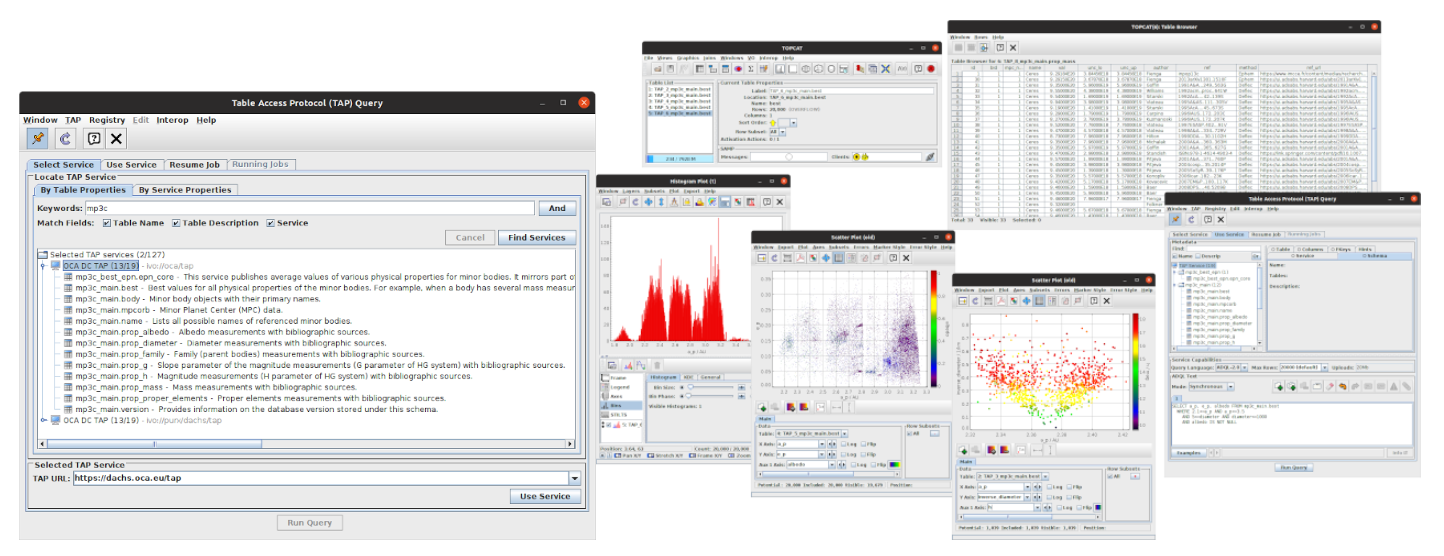
Figure 2: The MP3C service is accessible via the TAP protocol by the applications of the Virtual Observatory (here, TOPCAT). (Left) List of tables with their description, including the EPNCore table available in particular for the VESPA service. (Right) Graphs and tables obtained by submitting ADQL queries.
How to cite: Delbo, M., Avdellidou, C., Bruot, N., and Erard, S.: The Minor Planet Physical Properties Catalogue: Connection with the Virtual European Solar and Planetary Access of EUROPLANET and the big data challenge for planetary science, Europlanet Science Congress 2022, Granada, Spain, 18–23 Sep 2022, EPSC2022-323, https://doi.org/10.5194/epsc2022-323, 2022.
Abstract: The moon-coverage tool is a Python package currently used by ESA-SOC for the JUICE mission to plan and visualize Jupiter’s moons surface coverage. It supports instrument footprint projections and region of interest intersections.
Introduction: One of the key elements to assess the quality of an observation plan is to visualize its spatial coverage at different scales (global, regional and local). All the planetary missions, past, current and future use JPL/NAIF SPICE kernels to describe the position of the spacecraft and its orientation in space [1]. These files are usually produced by space agencies and require advanced users to interpret them to know when and how a given surface feature is visible on a planetary body.
A planning tool in Python: To simplify the identification of these opportunities, we developed the moon-coverage, a Python package built on top of spiceypy [2] that provides an object-oriented approach to perform spacecraft trajectory computations (Fig. 1), instrument field of view projections (Fig. 2) and region of interest intersections (Fig. 3). Originally developed for the ESA-JUICE mission, the tool can now handle any space mission (Europa-Clipper, BepiColombo, EnVision, Juno…).

Figure 1: JUICE temporal sequence of Europa flyby 7E1 (July 2nd 2032 with crema 5.0b23.1). The top panel represents the altitude of the spacecraft and the bottom the local incident angle. The orange color corresponds to the segment when the local incidence is lower than 90° (day side).
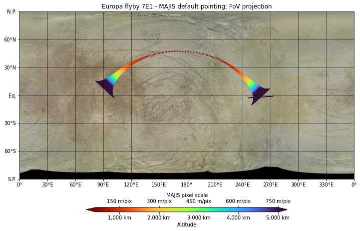
Figure 2: JUICE/MAJIS IR slit footprint during 7E1 flyby below 5,000 km. The trajectory is color-coded as a function of altitude and pixel scale.
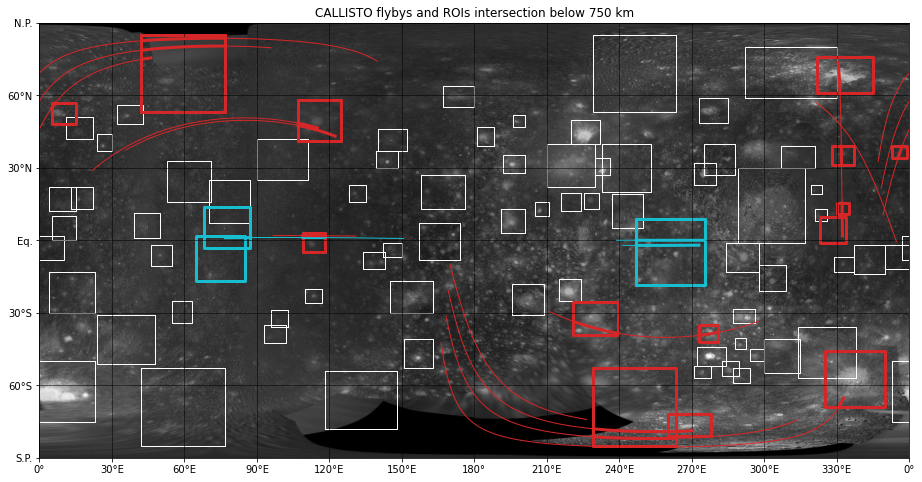
Figure 3: ESA/JUICE (red) and NASA/Europa Clipper (cyan) cumulative flybys over Callisto. The groundtrack below 750 km altitude are represented as solid lines. The large rectangles correspond to known regions of interest and are highlighted when the spacecraft groundtrack is intersecting them [3].
Resources: The source-code of the moon-coverage is publicly available on the JUICE Gitlab and distributed under open-source BSD license (https://moon-coverage.univ-nantes.fr). It is continuously tested on Python 3.8+ version and regularly deployed on PyPI. An extensive documentation is also available online with many examples than can be reproduced in Jupyter environments locally or ESA DataLabs.
Future developments: Currently the spacecraft/instrument pointing is based on the default camera kernels (ck). In a future release, we will allow the user to provide a Planning Timeline Request file (PTR) to perform custom adjustment of the attitude. We will also support planetary projections to display the result in polar/orthographic/sinusoidal views.
Acknowledgments: The moon-coverage is under active development at LPG (CNRS) and funded by ESA under 4000127262/19/ES/CM contract.
References: [1] Acton (1996) PSS, [2] Annex et al. (2020) JOSS, [3] Stephan et al. (2021) PSS
How to cite: Seignovert, B., Tobie, G., Vallat, C., Altobelli, N., and Belgacem, I.: The moon-coverage: a Python tool for mission and instrument planning, Europlanet Science Congress 2022, Granada, Spain, 18–23 Sep 2022, EPSC2022-341, https://doi.org/10.5194/epsc2022-341, 2022.
Spacecraft in the space environment plasma collect and emit charged particles ending charging themselves. Even with the best specification, the spacecraft potential charge to a potential of the order of the ambient electron temperature, which impact the instrument ability to investigate the thermal plasma characteristics. The most impacted instruments are the particle detector which see a distortion both in arrival direction and energy, and the plasma and field sensors which are perturbed by the electrostatic sheath around the spacecraft. In order to improve the space mission data analysis, the Spacecraft-Plasma Interaction Software (SPIS) has been developed by ONERA and Artenum, with support from the ESA, the CNES and the SPINE Community which gathers European academic and industrial partners and the charging issues. However, the precision of its modelings depends on the accuracy of its inputs, particularly concerning the plasma environment populations. In the frame of the Europlanet 2024 RI project funded by the European Commission, we developed a connection between SPIS and the main environment databases through the SPASE framework. Using the Simulation extension to SPASE, the IMPEX planetary environment simulation databases are also accesible. In addition, this extension allowed us to develop algorithms that allow to retrieve semi-automatically the data of interest (i.e. that can be exploited by software) in a whole database and to handle them properly. We will demonstrate the capability of the software - database connection to analyze instrument measurements and show the capability of SPASE to provide the metadata needed for the automatic processing of the data by client tools.
How to cite: Hess, S. and Leclercq, L.: Coupling the Spacecraft-Plasma Interaction Software to the Space Environment Databases, Europlanet Science Congress 2022, Granada, Spain, 18–23 Sep 2022, EPSC2022-347, https://doi.org/10.5194/epsc2022-347, 2022.
VESPA (Virtual European Solar and Planetary Access) has focused for 10 years on adapting Virtual Observatory (VO) techniques to handle Planetary Science data [1] [2]. The objective of this activity is to build a contributory data distribution system both to access and publish data with minimum fuss. This system is responsive to the new paradigm of Open Science and FAIR access to the data, and is optimized to publish data from public-funded programmes with limited resources.
VESPA’s architecture was defined during the previous Europlanet-2020-RI program, incorporating concepts and standards from various areas: astronomy, Earth observation, space physics, heliophysics, etc. It relies on the VO infrastructure: data services are installed in any location but are declared in a system of harvested registries with identifiers, end-point (URL), mention of supported access protocols, and a rough description of content. Such services are interoperable via clients and tools, which also provide visualization and analysis functions.
The activity in Europlanet-2024-RI focuses on expanding this environment, enforcing sustainability, and opening new possibilities to improve data handling – such as workflows, cloud-based computation, and readiness for exploitation through Machine Learning techniques.
Data access. VESPA uses a specific access protocol called EPN-TAP, associated with a metadata vocabulary providing uniform description of datasets in the field. At the time of writing EPN-TAP is in the final stage of becoming a Recommendation of the International Virtual Observatory Alliance (IVOA) [3].
EPN-TAP is compliant with the general TAP protocol, allowing usage of existing VO tools and communication protocols with data services pertaining to Solar System studies. Some VO tools (TOPCAT, Aladin, CASSIS) are also adapted to improve handling of such data, e.g. visualisation of footprints (spatial or temporal), reflected light, or spectral cubes on planetary surfaces. In parallel, OGC-compliant definitions of planetary coordinate reference systems will facilitate the use of GIS tools in Planetary Science.
The VESPA portal, intended as a discovery tool to browse the EPN-TAP services, is being redesigned to improve the user experience (new version expected to be released for the conference). Other, more specific access modes (via script, web services, Jupyter notebook, VO tools, etc) are also available.
Data services. 67 EPN-TAP data services are currently searchable from the VESPA portal, and about 20 are in development phase. Contributions from space agencies have increased significantly this year, with now 25+ million files in ESA’s PSA, and 60 datasets from the NASA PDS PPI node (declared in the IVOA registry but not yet reviewed for the portal). New services include atmospheric modelling from GCM (Venus and Mars), surface and asteroid spectra, radio observations, solar databases, and tables from published articles at CDS/VizieR. Larger data infrastructures with EPN-TAP interface (AMDA, SSHADE, PVOL) also develop their content and capacities, e.g. this year band lists have been implemented in SSHADE, and support for long time series in AMDA. An implementation workshop associated to a call for data services from the community was held in Nov 2021, and two more workshops are scheduled in the course of the programme.
Service implementation support. The standard procedure to implement services has been greatly enhanced with new releases of DaCHS (a VO data server by Heidelberg University) and TOPCAT (a VO tool for tabular data by the University of Bristol). Both tools fully support the current version of EPN-TAP and greatly facilitate the set-up of new data services: DaCHS includes a predefinition of standard EPN-TAP parameters (with units and UCDs), while TOPCAT includes an EPN-TAP validator. A Docker version of DaCHS is available for assessment purposes. Existing data services have been reviewed for compliance, and most of them have been upgraded to benefit from the latest developments. In many cases, their content has been extended with new data and functions.
Service access. The recent upgrade also addresses low-level technical aspects, e.g. related to declaration in the IVOA registry. Most EPN-TAP services are now declared in compliance with recent evolutions of the VO, and are findable independently from the portal.
Sustainability. Definition files of all services are stored in a unique gitlab for preservation and maintenance by several VESPA teams. Gitlab authentication is granted by GÉANT/eduTEAMS. This is a simple and efficient way to share the technical expertise among services and teams, and to improve sustainability.
Implementation of data services on EOSC (the recent European Open Science Cloud) was assessed during the VESPA-cloud project supported by EOSC-Hub, through its 2nd Early Adopter Program (2020-21). EPN-TAP services can be deployed on EOSC inside Virtual Machines or Docker containers, from the same gitlab installation used to preserve the services. This will provide a workaround to services temporary unavailability, for performing cloud-based computation on data services, and a solution for data providers who are not able or not willing to host a VESPA server for a long period of time.
Coming data services. Data produced by other WP in Europlanet-2024 will distribute their results using the VESPA infrastructure: other VAs (SPIDER, GMap, ML), NA2 (telescope network and other pro-am projects), and TAs (lab experiments and field studies). VESPA is of course also available to distribute data from other H2020 programmes in the field. An interface with space agency archives will make use of the recent PDS4 dictionary for EPN-TAP (in addition to the existing EPN-TAP interface on ESA’s PSA).
Prospects. Detailed examples of recent VESPA developments are provided in this session and related ones. The focus will shift again next year to new data services, with the finalization of several projects, in particular related to the Moon, Mercury, and exoplanets. A workflow platform will also be connected to perform run-on-demand (the OPUS system also used by the ESCAPE H2020 programme) and cloud-based activity will expand.
The Europlanet-2024 Research Infrastructure project has received funding from the European Union's Horizon 2020 research and innovation programme under grant agreements No 871149.
[1] Erard et al 2018, Planet. Space Sci. 150, 65-85. 10.1016/j.pss.2017.05.013. ArXiv 1705.09727
[2] Erard et al. 2020, Data Science Journal 19, 22. doi: 10.5334/dsj-2020-022.
[3] https://ivoa.net/documents/EPNTAP/
How to cite: Erard, S. and the VESPA team: Virtual European Solar & Planetary Access (VESPA) 2022: Sustainability, Europlanet Science Congress 2022, Granada, Spain, 18–23 Sep 2022, EPSC2022-676, https://doi.org/10.5194/epsc2022-676, 2022.
Introduction
The SSHADE database infrastructure (http://www.sshade.eu) hosts the databases of about 30 experimental research groups in spectroscopy of solids from 15 countries. It currently provides to all researcher over 5000 spectra of many different types of solids (ices, minerals, carbonaceous matters, meteorites…) over a very wide range of wavelengths (mostly X-ray and VUV to sub-mm)
However, although these data are invaluable for the community, one type of information is still critically missing to easily interpret laboratory, field or astronomical spectra: the list of the characteristics (band position, width, intensities, transition attribution, …) of the absorption bands of a given solid, called its ‘band list’.
This type of database is well developed for gases (see e.g. the VAMDC portal (2)), and it is even frequently the only type of spectral data available. But for solids (and liquids) there is currently almost no database which provides such information (only in some restricted fields, such as Raman spectroscopy of minerals, e.g. the WURM database (3)).
This critical lack triggered us to develop (within the Europlanet-2024 RI program) such a band list database containing the characteristics of electronic, vibration and phonon bands of various solids (ices, simple organics, minerals) of astrophysical interest to help:
- identify absorption or emission bands from solids observed in various astrophysical environments or in laboratory simulations
- determine the environment of the molecule or mineral (composition, isotopes, mixing, phase, T, P, …)
- select the best spectra in SSHADE to compare with observation, or to use in models
What is a band list of a solid?
A ‘band list’ is a list of band parameters and vibration modes of a molecule in a simple molecular constituent (3 species maximum), or of a mineral or a ionic/covalent solid, with a well-defined phase and composition (fixed or small range). It includes the bands of all isotopes (sub-bandlists) and can be provided for different environments (T, P, …).
The SSHADE 'band list' database provides the band parameters (position, width, peak and/or integrated intensity, and their accuracy, isotopic species involved, mode assignment, ...) of a progressively increasing number of solids and simple compounds (with different compositions) of astrophysical and planetary interest in various phases (crystallines, amorphous, ...) at different temperatures or pressures.
We are feeding this database through exhaustive compilations and critical reviews of all data published in various journals for pure ices and molecular solids and their simple compounds (solid solution, hydrates, clathrates, ...), including the own works of the SSHADE consortium partners. We will continue in a second step with band lists of minerals. However, this is a tremendous scientific work, expected to last many years… For example, the infrared spectrum of pure solid CO in its cubic α phase has been the subject of more than 35 papers scattered in 25 different journals over the period 1961-2020…
SSHADE band list database and interface
A specific data model, SSDM-BL (Solid Spectroscopy Data Model – Band List), has been first developed in order to accurately describe and link all the parameters necessary to describe both the solid constituent and the band list itself. A structured database storing all these data and metadata, has then be set up based on this data model. A data review tool (excel file), a data convertor to a XML import file, as well as a data import tool have been developed to feed the database.
Then an efficient search tool allows you to search either a band list or a specific band thanks to a combination between a ‘search bar’ and a set of filters on various parameters, such as band position, width and intensity, expected molecular or atomic composition, type of vibration, temperature and pressure. The search result are provided as a table with band list title or the main band parameters allowing the users to select the most relevant ones. He can then display the selected band list graphically, thanks to a simulator of ‘band list spectra’, with various unit and display options. The data can be exported as a table containing the main parameters of all the bands of the band list, as well as detailed metadata of the band list and all its bands. A data reference and a DOI will be associated with each band list.
SSHADE in Virtual Observatory
SSHADE-Bandlist will be later a service of the VESPA Virtual Planetary Observatory. It will be accessible via the EPN-TAP protocol, which will allow comparison with observational data and mass processing in the VESPA environment through a series of dedicated spectroscopy plotting and analysing tools.
Conclusion
This band list database should become a key tool for astronomers and planetary scientists to identify unknown absorption bands observed in the spectra of the surface or atmosphere of many astrophysical and solar system objects. Once the best candidate solid found by the user, the tool will link to the most relevant spectral datasets present in the SSHADE databases. These data can then be used for direct comparison with observations, or to model them through radiative transfer codes.
However its feeding will strongly depend on the scientific manpower available, and on the contribution of the SSHADE partners and of the community.
Acknowledgements
The Europlanet 2024 Research Infrastructure project received funding from the European Union's Horizon 2020 research and innovation programme under grant agreement No 871149. We also acknowledge OSUG, and INSU for additional financial supports.
References
- Schmitt, B., et al. (2018) SSHADE: "Solid Spectroscopy Hosting Architecture of Databases and Expertise" and its databases. OSUG Data Center. Service/Database Infrastructure. doi:26302/SSHADE
- Dubernet, M. L., et al. (2016). The Virtual Atomic and Molecular Data Centre (VAMDC) Consortium. Phys. B: At. Mol. Opt. Phys., 49, 074003 [doi:10.1088/0953-4075/49/7/074003]
- WURM project (http://www.wurm.info)
How to cite: Schmitt, B., Albert, D., Furrer, M., Bollard, P., Mandon, L., Gorbacheva, M., Bonal, L., and Poch, O.: SSHADE-BandList, the new database of spectroscopy band lists of solids, Europlanet Science Congress 2022, Granada, Spain, 18–23 Sep 2022, EPSC2022-778, https://doi.org/10.5194/epsc2022-778, 2022.
MITM12 | Planetary Missions, Instrumentations, and mission concepts: new opportunities for planetary exploration
Two 3-unit cubesats, FORESAIL-1 and ESTCube-2 soon to be launched (2022), both accommodate an electrostatic tether that can be charged to a high voltage with respect to the ambient ionospheric plasma in low-Earth orbit. The high voltage sheath around the tether serves as an electrostatic obstacle that perturbates the plasma ram flow causing Coulomb drag and a net braking force to reduce the orbital speed of the tether-spacecraft system.
According to the theory and particle-in-cell computer simulations, the Coulomb drag is a promising candidate for propellantless and continuous low-thrust propulsion in the solar wind with the plasma flow speeds typically being 440 km/s. In this presentation, we review its applications both to interplanetary missions as in ESA call for ideas, 2016, a 50-cubesat fleet to the main belt asteroids, and to space debris mitigation as in ESA cleansat building block 15, electrostatic tether plasma brake, 2017.
The key components of our payloads are a reeling system for the tether deployment and a high voltage power system: FORESAIL-1 (-1 kV); and ESTCube-2 (-1 kV, +0.5 kV, and +1.0 kV). In this presentation, we describe these payloads in further detail: The reeling system is such that the tether reel is supported by a ceramic bearing and rotated by a stepper motor and associated driver electronics. The 60-metre long tether is manufactured by knitting out of four thin aluminium wires with individual wire thickness of 50 micrometre. The multi-wire structure is required for redundancy against micrometeoroids. The tether is deployed by the centrifugal force provided by an end mass at the tip of the tether. During the launch, the reel and the end mass are secured by launch locks. The high voltage contact to the tether reel is realised by a slider connector. The payload electronics also contain the control electronics and electric power system. All this is miniaturised in order the payload spatial sizes to be less than that of one cubesat unit.
Concerning the high voltage polarity, the positive (negative) tether naturally collects electron (ion) current from the ambient plasma as electrons (ions) tend to neutralise the positive (negative) tether bias. Thus the high voltage system has to maintain the selected tether bias. In the solar wind, it is preferable to use the positive bias as it can be maintained by using electron emitters that are much simpler than the ion emitters. In the ionosphere, the plasma number density is large enough, and no ion emitter is required as an electron collecting surface as a conducting part of the spacecraft can be incorporated instead. For this reason, the payload on board ESTCube-2 has two electron emitters to enable the testing of the positive polarity high voltage system and the electron emitters for future development of the Coulomb drag propulsion in the solar wind. As a third topic of our presentation, the basics of the Coulomb drag propulsion are shortly covered.
Our tether payloads have been designed and built to measure the braking force caused by the Coulomb drag to the electrostatic tether in a low-Earth orbit plasma environment. It is a cornerstone measurement in the roadmap of evaluating Coulomb drag as space propulsion. On our roadmap, we are already developing a 6-unit cubesat (FORESAIL-2) for experiments in geostationary transfer orbit and further envisioning FORESAIL-3 and ESTCube-3, for example in lunar transfer orbit to measure the Coulomb drag in the solar wind.
How to cite: Toivanen, P., Janhunen, P., Kivekäs, J., Haslam, S., Polkko, J., and Iakubivskyi, I.: Cubesat experiments for Coulomb drag propulsion for interplanetary missions and space debris mitigation, Europlanet Science Congress 2022, Granada, Spain, 18–23 Sep 2022, EPSC2022-896, https://doi.org/10.5194/epsc2022-896, 2022.
Mutual impedance experiments are active electric instruments that provide in situ diagnostic in space plasmas, such as the plasma density and electron temperature. The instrumental technique is based on the coupling between electric antennas embedded in the plasma, and characterizes the local properties of the plasma dielectric.
Different versions of mutual impedance instruments are present onboard past and future planetary missions, such as Rosetta, BepiColombo, JUICE, and Comet Interceptor. Recently, the interest of the scientific community is shifting from large satellite platforms with single-point measurements concepts to small satellite platforms, to enable multipoint measurements for the spatial mappings of planetary outer environments. Therefore, instruments previously designed for large platforms are now miniaturized and adapted to small satellites. In this context, instrumental efforts are devoted to adapting mutual impedance experiments to small satellites, such as in the case of the CIRCUS CubeSat or the SPEED SmallSat missions projects.
Current state-of-the-art quantitative instrumental models of mutual impedance experiments are based on the assumption of an unmagnetized plasma. However, for planetary environments within which the magnetic field is not negligible, such as intrinsic planetary magnetospheres (e.g. Mercury, Ganymede) significant modifications of mutual impedance measurements are expected.
The goal of this work is twofold: (i) support the preparation of mutual impedance instruments for small satellites and (ii) extend current mutual impedance instrumental models to take into account the effects of the magnetic field on the plasma diagnostic.
This investigation is performed by combining two complementary approaches. First, numerical simulations are used to quantify the impact of the plasma magnetization on the mutual impedance measurements and, therefore, improve its diagnostic. In particular, we have developed and validated a new instrumental model, based on the numerical calculation of the electric potential emitted by an electric antenna in a magnetized, homogeneous, collisionless, Maxwellian plasma. This new instrumental model is used to compute synthetic mutual impedance spectra and assess the impact of electron magnetization on the instrumental response. Using this new model, we provide diagnostics for the plasma density, electron temperature, and magnetic field amplitude. Second, laboratory experiments are used to test and validate our numerical model. We use the controlled plasma environment of the PEPSO plasma chamber at LPC2E laboratory in Orléans. This plasma chamber offers the possibility to test the performances of space plasma instruments and CubeSats in realistic planetary ionospheric conditions. A model of CubeSat is present inside the plasma chamber, and is equipped with a set of electric antennas that are used to perform mutual impedance measurements in the same configuration as a CubeSat. The measurements obtained by this setup are compared with the instrumental model, to validate the plasma diagnostic of the instrument prototype on a CubeSat.
How to cite: Dazzi, P., Henri, P., Bucciantini, L., Lavorenti, F., Wattieaux, G., and Califano, F.: Mutual impedance experiments as a diagnostic for magnetized space plasmas, Europlanet Science Congress 2022, Granada, Spain, 18–23 Sep 2022, EPSC2022-1091, https://doi.org/10.5194/epsc2022-1091, 2022.
SB1 | Asteroid observations and modelling: properties and evolution of individual objects, families, and populations
Outer main belt asteroid (223) Rosa has been proposed as potential ESA JUICE mission flyby target of opportunity on its way to Jupiter (Avdellidou et al. 2021, Agostini et al. 2022). Rosa is a very dark (p < 0.05) object, with an effective diameter D of about 83 km. The very low albedo and the featureless red spectra indicate a P-type asteroid in the Tholen taxonomy, though the yet known bulk density estimates (2.0 ± 1.1 g cm−3 and 3.1 g cm−3; derived from masses by Fienga et al. 2019 and Park et al. 2021; see also Avdellidou et al. 2021) did not match very well this classification.
Aim of this work was to derive new estimates for the mass and for the bulk density for (223) Rosa. From the gravitational deflection on two small 'test' asteroids during close encounters with the perturber, namely (35525) 1998 FV64 on 2010-12-31.87 and (315162) 2007 FL24 on 2016-07-04.05, the mass of Rosa was derived as M = (3.62 ± 1.25) × 1017 kg (weighted mean of both results). This yields to a bulk density ρ = 1.2 ± 0.5 g cm−3, when adopting an effective diameter of D = 83 ± 8 km, as average of the available literature values. This density agrees well with typical densities for P-type asteroids like (87) Sylvia and (107) Camilla (ρ ≈ 1.3 g cm−3 ; see e.g. Carry et al. (2021), Vernazza et al. (2021)).
References
Agostini, L., Lucchetti, A., Pajola, M., et al. 2022, Planetary and Space Science, 216, 105476
Avdellidou, C., Pajola, M., Lucchetti, A., et al. 2021, A&A, 656, L18
Fienga, A., Deram, P., Viswanathan, V., et al. 2019, Notes Scientifiques et Techniques de l’Institut de Mecanique Celeste, 109
Carry, B., Vernazza, P., Vachier, F., et al. 2021, A&A, 650, A129
Park, R. S., Folkner, W. M., Williams, J. G., & Boggs, D. H. 2021, AJ, 161, 105
Vernazza, P., Ferrais, M., Jorda, L., et al. 2021, A&A, 654, A56
How to cite: Kretlow, M.: An astrometric mass estimate for asteroid (223) Rosa, Europlanet Science Congress 2022, Granada, Spain, 18–23 Sep 2022, EPSC2022-42, https://doi.org/10.5194/epsc2022-42, 2022.
The Gaia mission of the European Space Agency (ESA) was launched in December 2013 and began it scientific operations in July 2014. Gaia is essentially devoted to the measurement of positions, parallaxes, proper motions, brightnesses, and colours of stars. However, Gaia has also obtained astrometric, photometric, and spectroscopic measurements for several hundreds of thousands of asteroids.
The Gaia Data Release 3 (DR3) is the first to contain low resolution reflectance spectra of 60,518 solar system small bodies, the large majority of which are asteroids of the main belt (Gaia collaboration, Galluccio, Delbo et al. 2022). The global survey properties, the methods of data production and validation are detailed in the aforementioned paper published by the journal Astronomy and Astrophysics, which accompanies the DR3, and also summarised in the presentation of Galluccio et al. (2022) at this conference (EPSC 2022).
Here we present preliminary results about the Gaia view of asteroid collisional families. We identified asteroids belonging to families during the validation of Gaia asteroid spectra. Based on the family identification of Nesvorny et al. (2015), with the addition of the New Polana and the Eulalia families from Walsh et al. (2013), we found that in the Gaia DR3 there are 25,088 asteroids that belong to 116 collisional asteroid families of the 121 listed in Tab.1. This table also reports the number of family members and the number of members with a Gaia DR3 reflectance spectrum. However, the family identification of current catalogues is conservative by construction in order to keep good separation between the families. Hence, it is very likely that (i) some of the known families are more extended than what is available in current catalogues, namely, that catalogues based on dynamical criteria do not capture the whole extent of a family, and (ii) some unknown families are yet to be identified. This implies that the aforementioned number of asteroid family members with Gaia DR3 reflectance spectra is likely an estimation lower than the true number.
We will present some important features that Gaia observed in families. One of these is the correlation between some spectral parameters, such as the slope and the depth of the 1-micron absorption band of the reflectance spectrum, and the age of members of asteroid families belonging to the so called spectroscopic S-complex (DeMeo et al. 2009). These correlations can be explained in terms of a space weathering process that reddens and reduces the 1-band depth as a function of time on S-complex asteroids.
For the brightest asteroids, the extension of Gaia reflectance spectra at wavelengths shorter than 0.45 micron is very useful for distinguishing the composition of primitive, carbonaceous asteroid families, which are difficult to be discriminated with the ground based spectroscopic data currently present in the literature.
References:
- DeMeo, F. E., Binzel, R. P., Slivan, S.~M., Bus, S. J. 2009. Icarus 202, 160–180.
- Gaia collaboration, Galluccio, Delbo et al. 2022. A&A under review.
- Nesvorný, D., Brož, M., & Carruba, V. 2015. in Asteroids IV (P. Michel, et al. eds.) University of Arizona Press, Tucson.,
- Walsh, K. J., Delbo, M., et al. 2013. Icarus 225, 283–297.
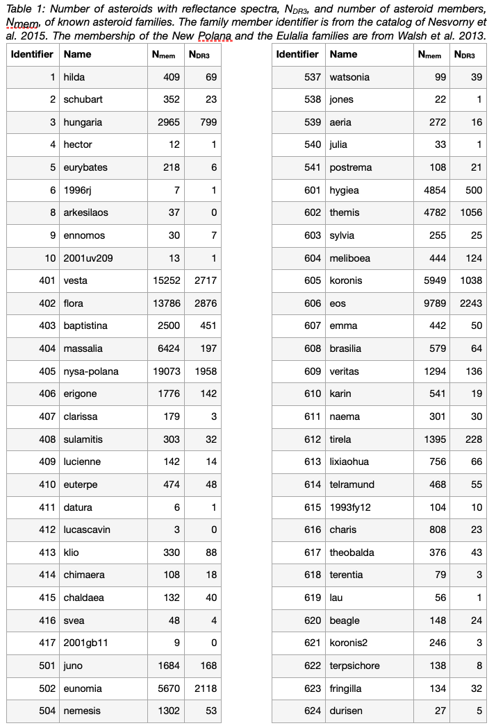
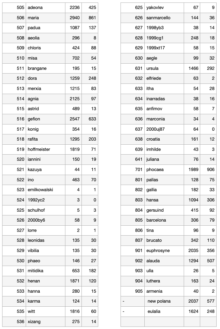
How to cite: Delbo, M., Galluccio, L., De Angeli, F., Pauwels, T., Tanga, P., Miagnard, F., Cellino, A., Brown, A., Muinonen, K., and Penttila, A.: Gaia spectroscopic view of asteroid collisional families: preliminary results, Europlanet Science Congress 2022, Granada, Spain, 18–23 Sep 2022, EPSC2022-237, https://doi.org/10.5194/epsc2022-237, 2022.
1. Introduction
Linear secular resonances occur when there is a commensurability between the frequency of precession of an asteroid perihelion, g, or node, s, and that of a planet. The ν6 involves a relationship between the frequency g of an asteroid and the g6 frequency of Saturn. Since it is a pericenter resonance, it can increase most asteroids’ eccentricities to planet-crossing levels. It can, therefore, destabilize most of the bodies that interact with it, and it is a major source of NEAs through Yarkovsky effect [2]. Despite this fact, stable orbital configurations exist inside the ν6 resonance. In such configurations, the resonant angle σ = ϖ −ϖ6, with ϖ the longitude of pericenter of the asteroid and ϖ6 that of Saturn, can oscillate around either 0◦ or 180◦. In the first case, we have an “aligned libration”, since the pericenters of both Saturn and the asteroid are pointing in the same direction. For the second case, we have an “anti-aligned libration”.
[4] identified the first case of an asteroid family completely made of asteroids in anti-aligned libration states, that of 1222 Tina. [6] extended this analysis to the whole main-belt, and found the first seven asteroids in aligned states of the same resonance. Here, we extended the previous analysis using the largest database of asteroid proper yet obtained.
2. Identification of the resonant population using large databases
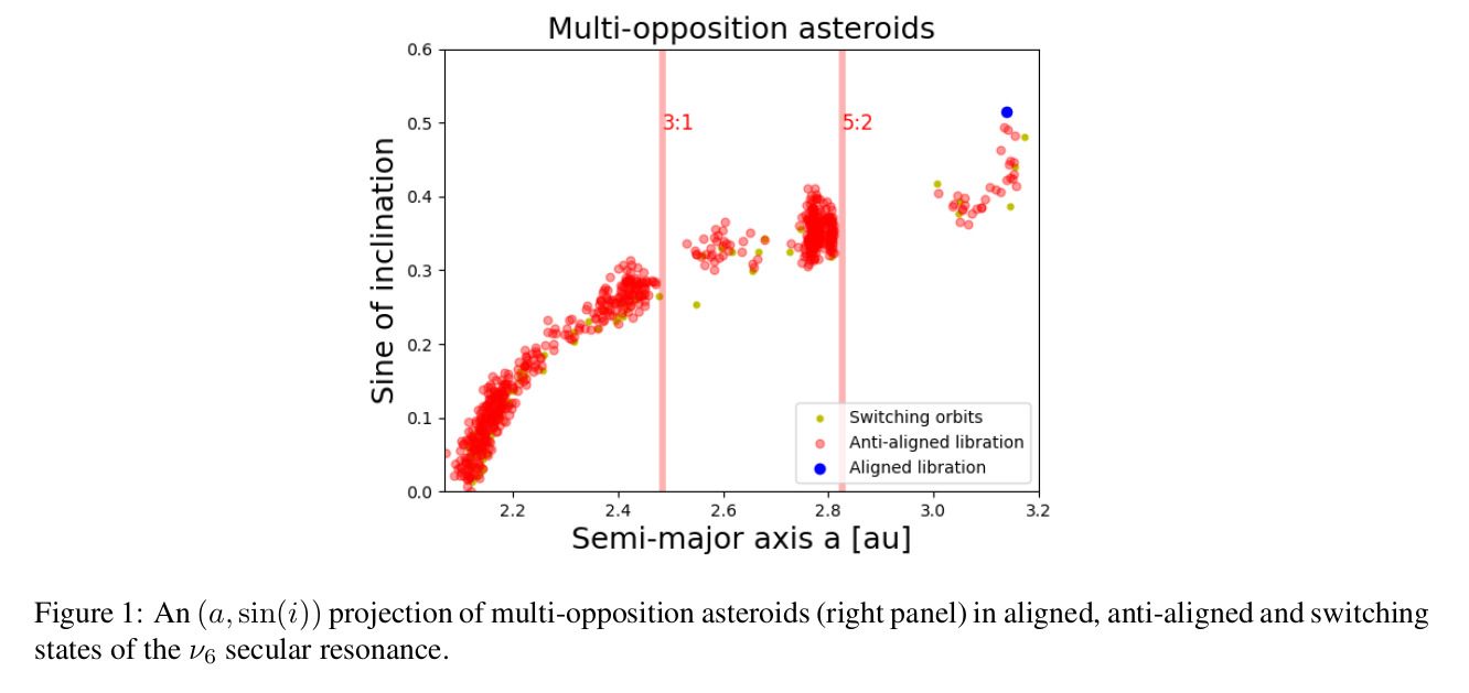
To identify the population of ν6 resonators, first, we need to select the asteroids most likely to be affected by this resonance. For this purpose, we use the criterion described in [6] and the approach outlined in [3]. We identified 15 asteroids on aligned orbital configurations, and 1713 on anti-aligned ones (see figure (1)). We then proceeded searching for asteroid groups among the newly identified anti-aligned population using the Hierarchical Clustering Method (HCM) [1]. Our results are shown in figures (2). We identify a new group around the asteroid 12988 Tiffanykapler.

3. 12988 Tiffanykapler: the first young family in the ν6 secular resonance
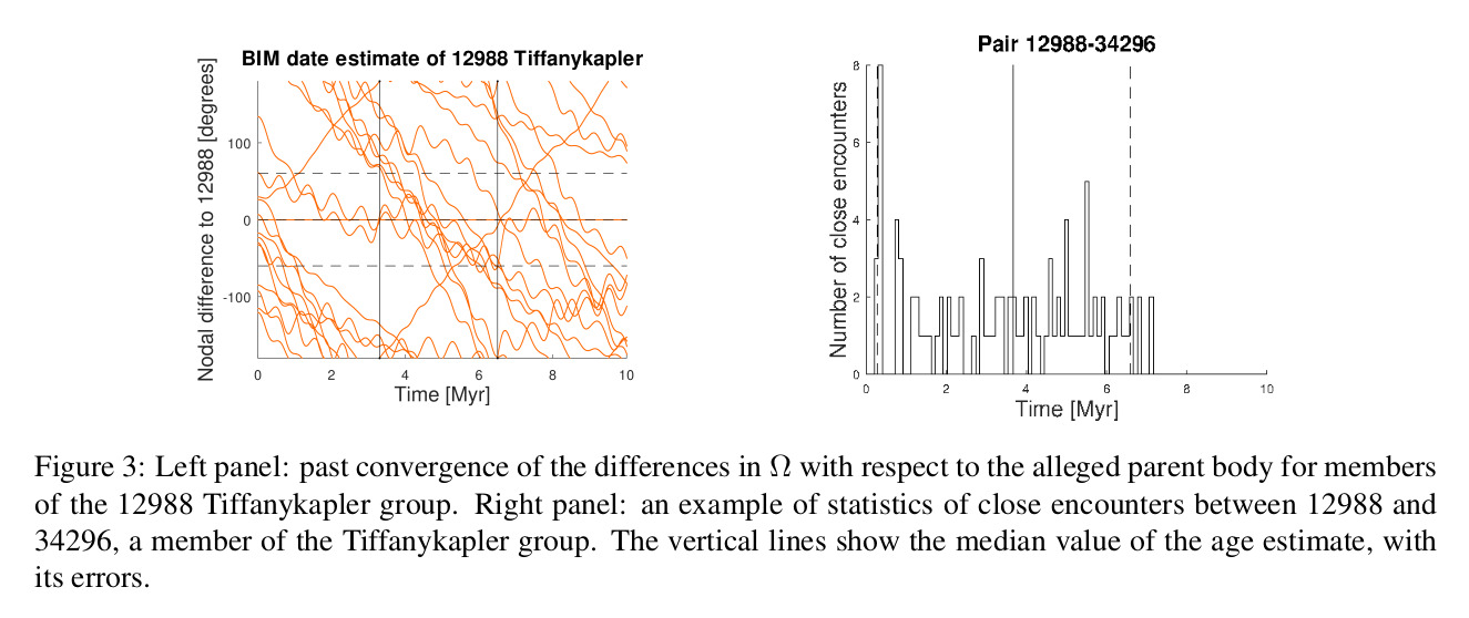
Young asteroid families can be dated using methods based on numerical integrations of family members in the past, like the Backward Integration Method (BIM, [7]) and the Close Encounters Method (CEM, [5]). In the BIM method, from time-reversal numerical simulations, past discrepancies in the longitudes of node Ω of family members with regard to those of the claimed parent body are obtained. These differences should converge to values approaching zero at the time of family formation. The CEM approach works by integrating into the past multiple clones of the parent body and of the other family members. Close encounters that occur at low relative distances and speeds between two clones are recorded, and the median value of these times is used to estimate the asteroid pair’s age. The results of both methods are shown in figure (3). The BIM method suggests a possible solution for the 12988 group in the time range from 3.3 to 6.5 Myr. The weighted average of the age determination of all asteroid pairs in the family, one example of which is shown in the right panel of figure (3), provides an age estimate for the family of 3.05 ± 1.15 Myr.
As discussed in [4], at the simplest level of perturbation theory the quantity:![]()
is preserved for asteroids in the ν6 resonance in the conservative case. The preservation of the original values of K2' permits to estimate the initial ejection velocity field with a method not generally available for non-resonant families. Our analysis yields a value of the ejection velocity parameter VEJ = 15+6-3 m/s.
4. Summary and Conclusions
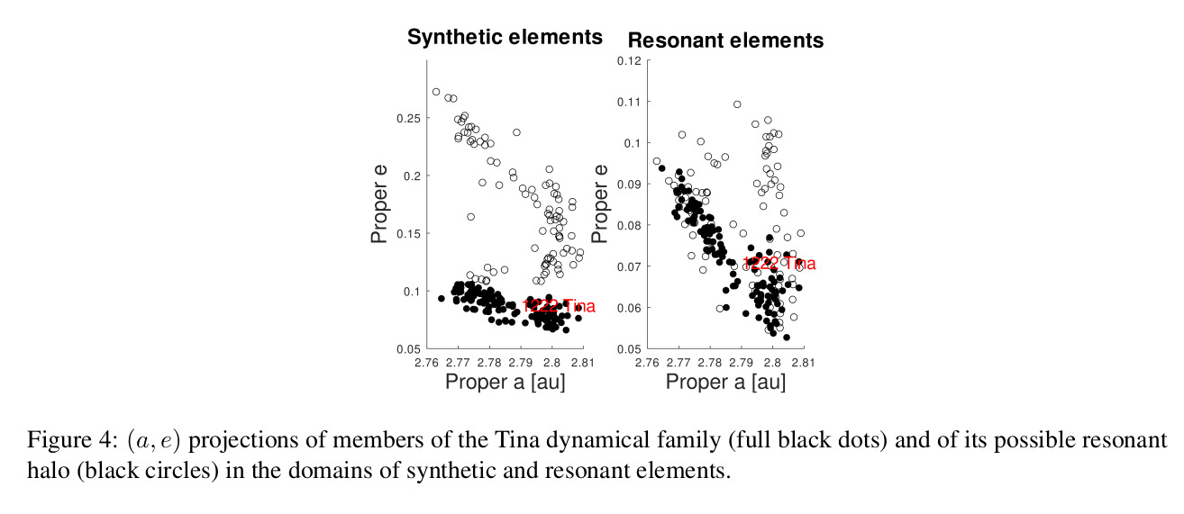
In this work, we were able to obtain a sample of 15 asteroids on aligned orbits and 1669 asteroids on anti-aligned orbits, the largest database so far for this asteroidal population. Two new asteroid groups were identified for the first time in this work: those of Tiffanykapler in the inner main-belt and 138605 QW177 in the outer belt. Tiffanykapler is the first young asteroid family in a linear resonant configuration ever to be found. Combining methods based on backward numerical simulations and constraints from resonant dynamics, we found that the family has an age of 3.05 ± 1.15 Myr and an ejection velocity field parameter of VEJ = 15+6-3 m/s. Finally, using resonant proper elements ([4]), we also identified a highly eccentric population of asteroids near the Tina family, that are likely to be part of its halo. It is the first example of a “resonant halo”.
Acknowledgements
We thank the Brazilian National Research Council (CNPq, grant 301577/2017-0), and the Foundation for Research Support of São Paulo state
(FAPESP, grant 2016/024561-0). More information on this work is available on Carruba et al. 2022, MNRAS, under review, available on ArXiv: 2203.15763.
References
[1] BENDJOYA, P., AND ZAPPALÀ, V. Asteroid Family Identification. In Asteroids III. Arizona Univ. Press, 2002, pp. 613–618.
[2] BOTTKE, W. F., JEDICKE, R., MORBIDELLI, A., PETIT, J.-M., AND GLADMAN, B. Understanding the Distribution of Near-Earth Asteroids. Science 288, 5474 (June 2000), 2190–2194.
[3] CARRUBA, V., A LJBAAE, S., DOMINGOS, R. C., AND BARLETTA, W. Artificial neural network classification of asteroids in the M1:2 mean-motion resonance with Mars. MNRAS 504, 1 (June 2021), 692–700.
[4] CARRUBA, V., AND MORBIDELLI, A. On the first ν6 anti-aligned librating asteroid family of Tina. MNRAS 412, 3 (Apr. 2011), 2040–2051.
[5] CARRUBA, V., S POTO, F., BARLETTA, W., ALJBAAE, S., FAZENDA, Á. L., AND MARTINS, B. The population of rotational fission clusters inside asteroid collisional families. Nature Astronomy 4 (Jan. 2020), 83–88.
[6] HUAMAN, M., ROIG, F., CARRUBA, V., DOMINGOS, R. C., AND ALJBAAE, S. The resonant population of asteroids in librating states of the ν6 linear secular resonance. MNRAS 481, 2 (Dec. 2018), 1707–1717.
[7] NESVORNÝ, D., BOTTKE, WILLIAM F., J., DONES, L., AND L EVISON, H. F. The recent breakup of an asteroid in the main-belt region. Nature 417, 6890 (June 2002), 720–771.
How to cite: Carruba, V., Aljbaae, S., Domingos, R. C., Huaman, M., and Martins, B.: Identifying the population of stable ν6 resonant asteroids using large databases, Europlanet Science Congress 2022, Granada, Spain, 18–23 Sep 2022, EPSC2022-238, https://doi.org/10.5194/epsc2022-238, 2022.
1. Introduction
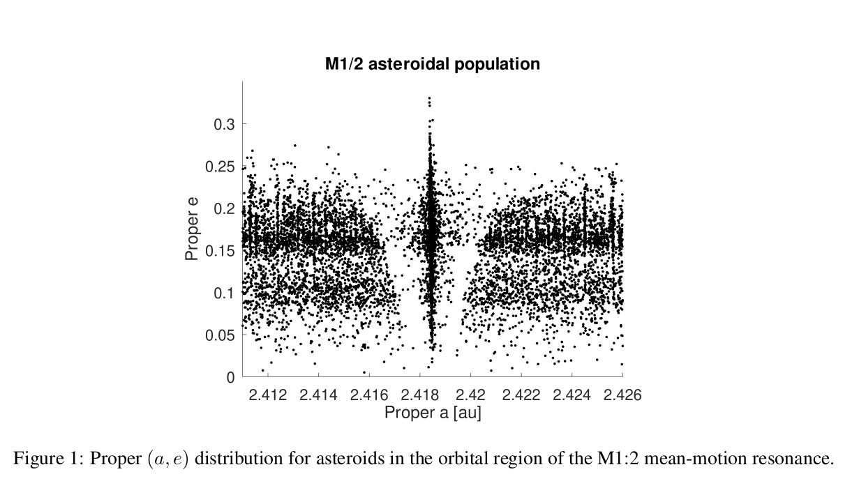
During the last five years, machine learning and deep learning have been used more commonly in the field of asteroid dynamics. Artificial neural networks have been recently used for identifying members of asteroid families [6]. This is the first attempt to use deep learning for the automatic classification of images of asteroids resonant arguments. The population of asteroids inside the M1:2 mean motion resonance with Mars was studied by [4]. The V-shaped region at the resonance center in the proper (a, e) plane (see figure (1)) is associated with the M1:2 resonance. [4] defines two main resonant arguments. σ is given by:
![]()
where λ = M + Ω + ω is the mean longitude, ϖ = Ω + ω, with Ω the longitude of the node, ω the argument of pericenter, and where the suffix M identifies the planet Mars. σ1 is defined as:
![]()
The orbital behavior of asteroids in the affected region can be identified by studying the time dependence of these two angles. Asteroids for which the critical arguments cover the whole range of values, from 0◦ to 360◦, are on circulating orbits. If the argument oscillates around an equilibrium point, we have a librating orbit. Whether the argument alternates phases of libration and circulations we have a switching orbit, as defined in this work. The main equilibrium point for the σ1 argument is near 0◦. Pure σ librators tend to be much rarer than pure σ1 ones. Since in this work we are interested in treating a multi-class problem we focus our study on the case of the σ1 resonant argument.
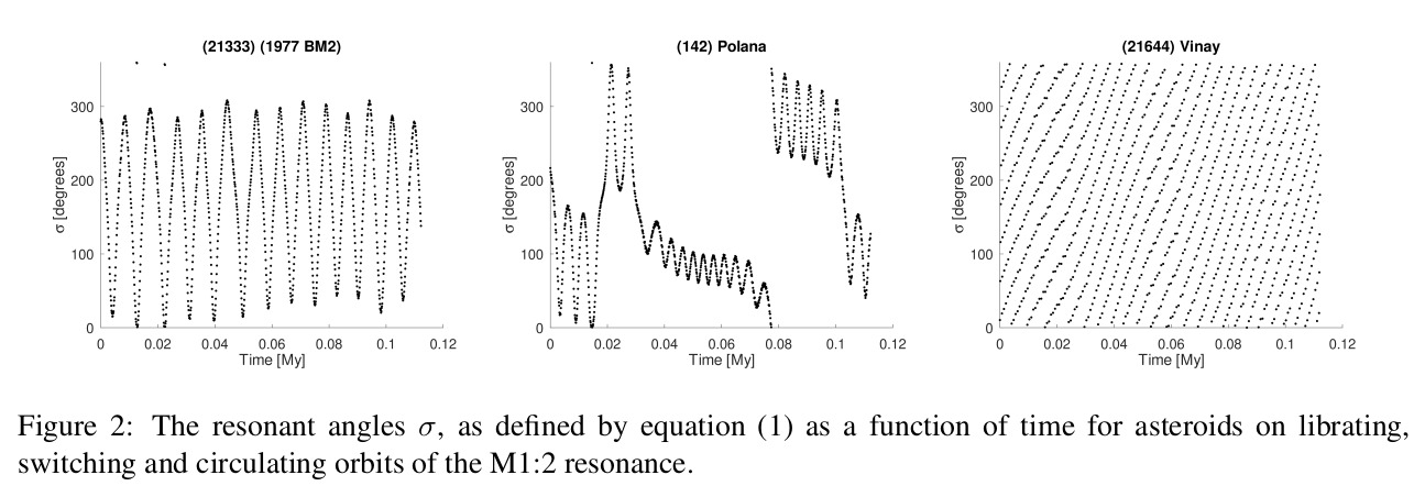
2. Artificial Neural Networks (ANN)
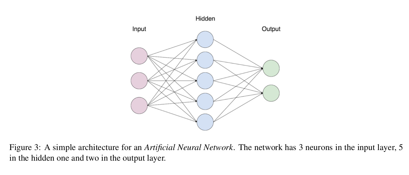
Artificial neuron networks mimic the neuron's web in a biological brain. Each artificial neuron can transmit a signal to other neurons. This signal can be processed, and the signal coming out of each neuron is computed as a non-linear function of the inputs. A basic architecture for ANN consists of an input and an output layers, with the possible presence of one or more hidden layers between them to improve the model precision. Each neuron will perform a weighted sum, WS, given by:

where n is the number of input to process, Xi are the signals from other neurons, and wi are the weights. ANN will optimize the values of the weights during the learning process. On the weighted sum WS, ANN will apply an activation function. For images classifications, one of the most used activation function is the “relu”, defined as:
![]()
which will produce as an outcome the weighted sum itself WS, if that is a positive number, or 0, if WS has a negative value. As a next step, the loss function must be applied to all the weights in the network through a back-propagation algorithm. A loss function is usually calculated by computing the differences between the predicted and real output values. Interested readers can find more information in the Keras documentation (https://keras.io/, [5]).
3 Applications of ANN to M1:2
Here, we used the Keras implementation of ANN, which is based on the Tensorflow Python software package [2]. The process used in this work is the following:
1. The asteroid orbits are integrated under the gravitational influences of the planets.
2. We compute the resonant arguments.
3. Images of the time dependence of resonant arguments are drawn.
4. The ANN trains on the training label image data.
5. Predictions on the test images are obtained, and images of the test data, with their classification, are produced.
To identify resonant argument images, we created a four-layer model with a flatten, an inner, a hidden, and an output layers. The flatten layer will transform the image matrices into arrays. The inner layer will look for simpler patterns in the arguments images, while the hidden layer will search for more complex features. The output layer, with three nodes, will perform the final classification for the three possible classes. To quantitatively classify the outcome of ANN, it is often useful to compute values of metrics. [3] defines accuracy as:

Our model performs quite well: Accuracy values were all above 0.996.
4. ML identification of resonant groups
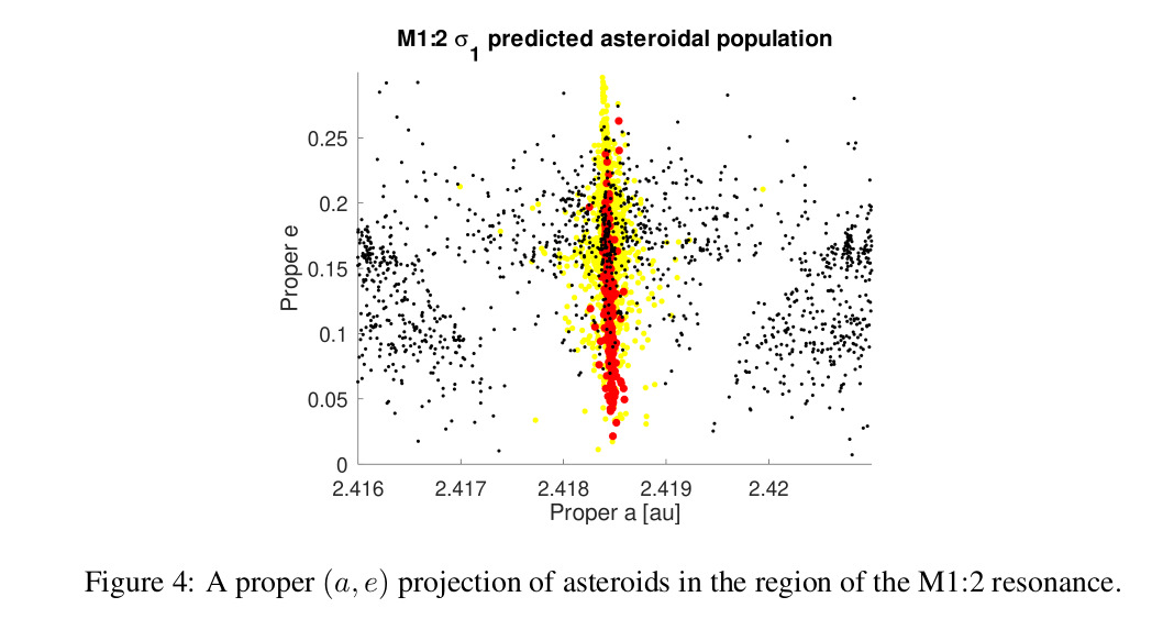
Using ANN and ML, we obtained labels for 6440 asteroids in the M1:2 resonance region. We then used the ML Hierarchical Clustering Method (ML-HCM) of [1] to identify asteroid groups among the resonant population of M1:2 resonators. Our analysis produced seven possible groups, all associated with the Massalia, Nysa, and Vesta families. This confirms the analysis of [4].
5. Summary and Conclusions
The use of ANN allowed us to classify the orbital type of all numbered asteroids affected by the M1:2 resonance. The identification of clusters in the population of asteroids in librating and switching orbits suggested that three asteroid families, those of Massalia, Nysa, and Vesta, are the most dynamically affected by this resonance.
Acknowledgements
We would like to thank the Brazilian National Research Council (CNPq, grant 301577/2017-0). More information on this work can be obtained from Carruba et al. (2021), MNRAS, 504, 692.
References
[1] CARRUBA, V., ALJBAAE, S., AND LUCCHINI, A. Machine-learning identification of asteroid groups. MNRAS 488, 1 (Sept. 2019), 1377–1386.
[2] CHOLLET, F., AND OTHERS. Keras: The Python Deep Learning library, (June 2018).
[3] FAWCETT, T. An introduction to ROC analysis. Pattern Recognition Letters 27, 8 (Jun. 2006), 861 –874.
[4] GALLARDO, T., VENTURINI, J., ROIG, F., AND GIL-HUTTON, R. Origin and sustainability of the population of asteroids captured in the exterior resonance 1:2 with Mars. Icarus 214, 2 (Aug. 2011), 632–644.
[5] LECUN, Y., BENGIO, Y., AND HINTON, G. Deep learning. Nature 521, 7553 (May 2015), 436–444.
[6] VUJIČIĆ, D., PAVLOVIĆ, D., D., M., Ð ORÐEVIĆ, S., S., R., AND D., S. Classification of asteroid families with artificial neural networks. Serb. Astron. J. 200 (Dec. 2020), 1–8.
How to cite: Carruba, V., Aljbaae, S., Domingos, R. C., and Barletta, W.: Artificial Neural Network classification of asteroids in the M1:2 mean-motion resonance with Mars., Europlanet Science Congress 2022, Granada, Spain, 18–23 Sep 2022, EPSC2022-245, https://doi.org/10.5194/epsc2022-245, 2022.
Introduction
The main belt asteroid 4429 Debussy belongs to a unique group among binary asteroids in the Solar System which are known as synchronous binary, the systems with two bodies having comparable sizes and with the same rotational and orbital period. Photometric observations of these objects are still the main source of their physical properties. Lightcurves for synchronous binary systems are not quasi-sinusoidal as for most asteroids, but have very characteristic U-V shape due to the rotation of nonspherical bodies and caused by mutual eclipses. The collection of data from apparitions over several years (evenly distributed along the ecliptic longitudes), allows to determine key parameters of such binary systems (such as a non-convex shape solution and the object's spin-axis orientation) (Bartczak et al., 2014, Bartczak et al., 2017, Kryszczyńska et al., 2008).
The ultimate goal of this kind of sophisticated spin-shape modeling is to determine the asteroid's density. It is indicative of the internal structure of the body and also puts constraints on its composition. However, the estimation of density is based on mass and volume. The determination of the volume of an asteroid requires a detailed shape solution, and information about the absolute size. Our main goal of modelling Debussy is calculating a new non-convex model with its uncertainties, which are crucial in further analysis (like radiometric studies) and for the estimation of other parameters (like thermal surface properties or bulk density).
4492 Debussy
The binary nature of Debussy was discovered in 2002 (Behrend et al., 2004), when photometric observations showed a lightcurve with typical features for eclipsing binaries - the amplitude of light changes (of about 0.5 mag) corresponding to the rotation of two nonspherical bodies, and two minima (about 0.6 mag deep) due to their mutual eclipses. Further observations showed that the rotation period is P = 26.5811 ± 0.0002 h (Polińska et al., 2008). Since 2002 Debussy has been observed at almost all ecliptic longitudes evenly distributed along the orbit. All gathered data present lightcurves with deep minima caused by mutual eclipses. This means that the edge of the orbit of the binary system always points towards the observer.
Modelling
The spin-shape model of the Debussy system is calculated in the same way as for 90 Antiope (Bartczak et al., 2014) and 809 Lundia (Bartczak et al., 2017, Kryszczyńska et al., 2008), using the genetic-algorithm-based modelling method SAGE (Shaping Asteroids with Genetic Evolution). The SAGE method is based on photometric observations from several apparitions. The modelling process works best for observations obtained with different and evenly distributed ecliptic longitudes. It allows to create non-convex shape, spin axis orientation and rotational period of synchronous binary asteroids. With the new model we would like to demonstrate the recently developed shape uncertainty method for binary objects in the same way as it was done for single asteroids and described in Bartczak & Dudziński (2019).
4492 Debussy was detected in the AKARI infrared survey and also during the cryogenic phase of WISE (calibrated fluxes were taken from the Database for thermal IR observations of small bodies, see Szakats et al. 2020). In addition, there is a dedicated Spitzer-IRS spectrum available (Marchis et al. 2012). We used the available thermal measurements to determine the size (size of an equal-volume sphere), the geometric albedo and the thermal inertia of Debussy via a well-tested thermophysical model (see e.g., Müller et al. 2017). For the radiometric study, we considered Debussy's derived spin properties, as well as different simple, convex, and non-convex shape solutions.
References
Behrend et al., 2004, IAU Circ., No. 8354
Bartczak et al., 2014, MNRAS, 443, 1802
Bartczak et al., 2017, MNRAS, 471, 1, 941-947
Bartczak P. & Dudziński G., 2019, MNRAS, 485, 2, 2431-2446
Kryszczyńska et al., 2008, A&A 501, 769-776
Marchis et al. 2012, Icarus 221, 1130
Müller et al. 2017, A&A 599, A103
Polińska et al., 2008, ACM paper id. 8134
Szakats et al. 2020, A&A 635, A54
How to cite: Polińska, M., Bartczak, P., and Müller, T. and the SAGE Team: New modeling of 4492 Debussy eclipsing binary asteroid, Europlanet Science Congress 2022, Granada, Spain, 18–23 Sep 2022, EPSC2022-286, https://doi.org/10.5194/epsc2022-286, 2022.
Our understanding of Solar System family asteroids has been significantly widened by space surveys primarily targeted to exoplanet detections. In K2 and TESS fields, many asteroids passed through, being a basis of continuous sateroid photometry covering several basis. This enabled the proof
of the high fraction of slow rotators (period>30 hours) in asteroid families (30%), non-family MB asteroids (35%), the Hilda group (39%) and the Trojan swarms (25%). High ratio of extremely slow rotators (P > 100 hr) in the Hilda group is (18%) is unique in the Solar System.
We found a family-specific amplitude and/or period distribution only in some asteroid families (Hungaria, Maria, Juno, Eos, Eucharis, and Alauda). Older families tend to contain a larger fraction of more spheroidal, low-amplitude asteroids. The rotation period distributions are different in the cores and outskirts of the Flora and Maria families, while the Vesta, Eos, and Eunomia families lack this feature. We also confirm that very fast spinning
asteroids are close to spherical (or spinning top shapes), and minor planets rotating slower than ≈11 h are also more spherical than asteroids in the 4-8 h period range and this group is expected to contain the most elongated bodies.
Despite a previously suggested mixed origin of Hildas from the MB and the Trojan swarms, we revealed no differences in the photometric properties between the taxonomically different R and LR Hildas: the entire Hilda group highly resembles the Trojans for rotational properties.
How to cite: Szabó, G.: Rotational properties of MB family asteroids, Hildas, and Trojans, based on K2 and TESS observations, Europlanet Science Congress 2022, Granada, Spain, 18–23 Sep 2022, EPSC2022-293, https://doi.org/10.5194/epsc2022-293, 2022.
The classification of the minor planets of the Solar System has been revisited regularly since its first outline in the 1970s as dichotomy of carbonaceous and silicaceous asteroids. The reformulations followed insights granted by new data (e.g. surveys such as ECAS, SMASS) or extensions of the observable feature space (e.g. CCD spectroscopy).
Since the last major update of the taxonomy by DeMeo et al. in 2009, we have seen a wealth of new data provided by targeted campaigns, which show that the spectroscopically-defined class boundaries do not align sufficiently with mineralogical and meteoritic population trends. Examples are the continuous trend between B- and C-type objects (Clark et al. 2010, De Leon et al. 2012) and the large subclassing of the continuous S-type asteroids (Vernazza et al. 2014). Furthermore, any compositional interpretation of members of the X-complex is tentative as shown by the diversity of radar albedos, densities, and spectral properties observed among them (Shepard et al. 2010, 2015, Carry 2012, Neeley et al. 2014).
Given the increase of data and insights into the compositional asteroid Main Belt, we derive a new iteration of the asteroid taxonomy, focusing primarily on a methodological improvement. Acknowledging that future survey efforts will contribute asteroid spectra in different wavelength ranges (e.g. Gaia (visible), SPHEREx (NIR), MITHNEOS (visible-NIR)), we evolve the current method into a probabilistic model approach which enables us to classify complete and partially observed spectra in the same scheme. We further re-introduce the visual albedo into the classification space to disentangle the degenerate X-complex.
By means of a clustering analysis of almost 3,000 minor body spectra and albedos, we devise a taxonomic scheme consisting of 17 classes with close resemblance to the Bus-DeMeo and Tholen systems (refer to Fig. 1): A, B, C, Ch, D, E, K, L, M, O, P, Q, R, S, X, V, Z. The two main complexes remain C and S. We resolve the X-complex and replace it by the new M-complex. Subclasses in the Bus-DeMeo system are replaced by a mineralogical interpretation of the continuous distribution of minor bodies in the classification space. The new class Z entails extremely-red objects in the inner Main Belt including the supposed TNO-implants (203) Pompeja and (269) Justitia (Hasegawa et al. 2021).
A python-tool to classify minor body observations in the derived taxonomic scheme is freely accessible to the community (https://classy.readthedocs.io).

Figure 1: Evolution of the asteroid taxonomy from the Tholen- (Tholen 1984) over the Bus-DeMeo- (Bus and Binzel 2002, DeMeo et al. 2009) to the system established in this work.
References
Clark, B. E., Ziffer, J., et al. (2010), Spectroscopy of B-type asteroids: Subgroups and meteorite analogs.
Carry, B. (2012), Density of asteroids.
Bus, S. J. and Binzel, R. P. (2002), Phase II of the Small Main-Belt Asteroid Spectroscopic Survey. A Feature-Based Taxonomy.
DeMeo, F. E., Binzel, R. P., et al. (2009), An extension of the Bus asteroid taxonomy into the near-infrared.
de León, J., Pinilla-Alonso, N., et al. (2012), Near-infrared spectroscopic survey of B-type asteroids: Compositional analysis.
Hasegawa, S., Marsset, M., et al. (2021), Discovery of Two TNO-like Bodies in the Asteroid Belt.
Neeley, JR., Clark, BE., et al. (2014), The composition of M-type asteroids II: Synthesis of spectroscopic and radar observations.
Shepard, M. K., Clark, B. E., et al. (2010), A radar survey of M- and X-class asteroids II. Summary and synthesis.
Shepard, M. K., Taylor, P. A., et al. (2015), A radar survey of M- and X-class asteroids. III. Insights into their composition, hydration state, & structure.
Vernazza, P., Zanda, B., et al. (2014), Multiple and Fast: The Accretion of Ordinary Chondrite Parent Bodies.
How to cite: Mahlke, M., Carry, B., and Mattei, P.-A.: A New Iteration of the Asteroid Taxonomy, Europlanet Science Congress 2022, Granada, Spain, 18–23 Sep 2022, EPSC2022-385, https://doi.org/10.5194/epsc2022-385, 2022.
Asteroids, along with other small bodies, are what is left over of the original planetesimal disk from the planet-formation era. Therefore, these objects are considered the best tracers for the processes that occurred during the earliest history of our Solar System. However, the majority of asteroids are fragments generated by the collisional breakup of the planetesimals, the first ~100-km sized bodies (Morbidelli et al., 2008, Delbo' et al., 2019) that accreted in the protoplanetary disk of our Sun.
Nevertheless, a small fraction of the planetesimal population survived the collisional evolution. In order to study these objects, the first step is to identify these surviving planetesimals among all the other (fragment) asteroids. To do so, we “cleaned” the inner part of the asteroid main belt (2,1 < a < 2,5) from all asteroid collisional family members (using the method of Bolin et al., 2017, Delbo' et al., 2017, 2019), thus revealing those asteroids that are not fragments that formed in the main belt. Thanks to this method, we revealed 64 surviving planetesimals in the inner main belt.
We carried out a spectroscopic survey of these identified IMB planetesimals, in order to constrain their composition and mineralogy. In particular, we performed visible and near-infrared spectroscopy using several telescopes such as the 1.82m Copernico Telescopio (Asiago, Italy) for the visible spectroscopy and the 4.2 Lowell Discovery Telescope (Flagstaff, USA); the 3.2 NASA Infrared Telescope Facility (Hawaii, USA) and the Telescopio Nazionale Galileo (La Palma, Spain) for the near-infrared part. To complete our survey, we also used spectra in the visible and near-infrared published in the literature, as well as size and albedo information that we obtained from the Minor Planet Physical Properties Catalog (https://mp3c.oca.eu/).
We performed the taxonomic classification following the Bus-DeMeo taxonomy (Bus et al., 2002; DeMeo et al., 2009), and using the M4AST tool (http://m4ast.imcce.fr) (Popescu et al., 2012). A visual inspection to identify the presence of absorption bands characteristic of some classes was performed to check the robustness of the automatic taxonomic classification. In addition, we compute for each planetesimal several spectral parameters, such as spectral slopes, and center, depth and area of absorption bands, when these are present. We also performed calculation of their mass, based on the method of (Carry, 2012). Finally, we used the RELAB database (Pieters, 1983), to look for meteorite analogues of each planetesimal.
We found that planetesimals of the Inner Main Belt (IMB) belong mainly to the S-complex (~45%), followed by C-complex (~25%) and X-complex (~17%). Further investigations on S-complex planetesimals showed that, for a majority of them, they are best matched by spectra of ordinary chondrites meteorites. We did not find any correlation with diameters, semimajor axis and the ratio of olivine/pyroxene. Almost 60% of the C-complex planetesimals belong to the Ch/Cgh types, showing spectroscopic features associated with hydrated minerals, and consequently indicating the presence of liquid water in the early formation phases of these objects. We also found that almost 5% of the IMB planetesimals belong to the D/T types with a diameter greater than 25 km. As this taxonomical class, as well as Ch/Cgh types, are likely to have formed in the outer part of the Solar System (at 3-7 au), their presence in the IMB (2,1-2,5 au) can be explained by dynamical models invoking large semimajor axis migration of these objects (e.g., Grand Tack of Walsh et al., 2011; low-mass asteroid belt of Raymond and Izidoro, 2017b for the C-complex and Vokrouhlický et al., 2016 for the D/T types).
Here, we will present the spectroscopic, physical and compositional results of our IMB planetesimals survey as well as the implications for planetary formation models.
Acknowledgements: We acknowledge support from the ANR ORIGINS (ANR-18-CE31-13-0014).
References : Morbidelli A. et al, Physica Scripta, Volume 130, Issue, id 014028 (2008) ; Delbo M. et al., A&A, Volume 624, id. A69 (2019) ; Bolin B. T. et al., Icarus, Volume 282, 2017, Pages 290-312 ; Delbo M. et al., Science, Volume 357, Issue 6355, pages 1026-1029, (2017) ; Bus S. J. et al., Icarus, Volume 158, Issue 1, Pages 146-177 (2002) ; DeMeo F. E. et al., Icarus, Volume 202, Issue 1, Pages 160-180 (2009); Carry, B. Planetary and Space Science, Volume 73, Issue 1, p. 98-118. (2012) ; Popescu M. et al., A&A, Volume 544, id. A130 (2012) ; Pieters, C. M., J. Geophys. Res., Volume 88, pages 9534– 9544 (1983) ; Walsh K. J. et al., Nature, Volume 475, Issue 7355, Pages 206-209 (2011) ; Raymond S. N. et al., Science Advances, Volume 3, Issue 9, Pages e1701138 (2017) ; Vokrouhlický D. et al., The Astronomical Journal, Volume 152, Issue 2, id. 39 (2016).
How to cite: Bourdelle de Micas, J., Fornasier, S., Delbo, M., Avdellidou, C., Van Belle, G., and Ochner, P.: Composition of Inner Main Belt Planetesimals, Europlanet Science Congress 2022, Granada, Spain, 18–23 Sep 2022, EPSC2022-440, https://doi.org/10.5194/epsc2022-440, 2022.
We report an analysis of photometric observations for two potentially hazardous asteroids – (52768) 1998 OR2 and (99942) Apophis. Data for 1998 OR2 was obtained in March – April 2020 and for Apophis in February – March 2021, when both objects experienced their close approaches to Earth. The aim of the observations was mainly to refine the physical characteristics (rotation periods, absolute magnitudes H, slope parameter G, to find out the approximate taxonomy, or even to estimate the heliocentric position of the north pole).
Observations and data reduction
The observations of both PHAs were carried out with the 0.61-m f/4.3 Newton reflector at the Skalnaté Pleso Observatory (Slovakia, IAU code 056) and CCD camera SBIG ST-10XME. We obtained photometric data using broad-band Johnson-Cousins B, V, and R filters, 2×2 binning, and a resolution of 1.07 arcsec/px. The calibration with dark and flatfield frames was applied in the standard way. Next, we used a differential aperture photometry technique to obtain lightcurves.
Results
Asteroid 1998 OR2 was observed for 9 nights. From each night we obtained 3 – 4 hr series in BVR filters, from which we determined the exact synodic rotation periods. Figure 1 shows the composite light curves with periods of 4.11 hours. We divided them into three groups to emphasize the time- and phase-angle-dependent changes in the lightcurve shape.
Data from the V filter we used to determine the absolute magnitude H, which has a value of 15.72 ± 0.02 mag (Fig. 2). We kept the slope parameter G at 0.15 because of the narrow range of phase angles. Next, we calculated the approximate effective diameters of the asteroid using an albedo value of 0.2. These varied only minimally between 2.1 and 2.3 km on each observing night, with a mean value of 2.14 ± 0.06 km.
Color photometry also allowed us to determine an approximate taxonomic class in the Tholen classification. Figure 3 shows the positions of the color indices on each night along with the mean value of the B-V and V-R indices. With high probability, the asteroid surface is dominated by a metallic material, which characterizes the X-class. Our finding is confirmed by Hromakina et al. (2021) [2].
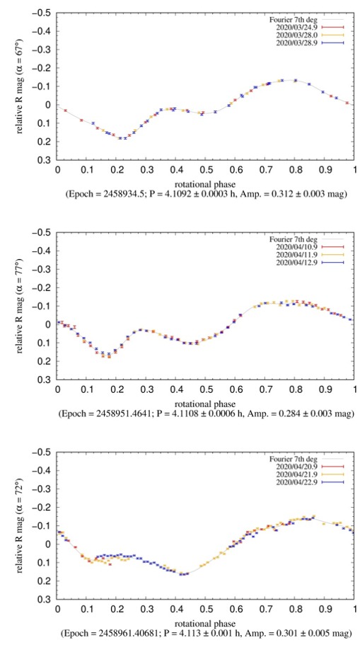
Fig. 1 Three composite lightcurves of asteroid 1998 OR2 obtained from March 24 to April 22 through the R filter. We divided them into three groups to show the changing of some features in brightness in the range of rotational phase from 0 to 0.2. All lightcurves have the same scale of relative magnitudes (y-axis) for better comparison. The typical rms of all composite lightcurves is less than 0.010 mag.

Fig. 2 Plot of magnitude-phase relation of 1998 OR2. In this case, the slope parameter G is fixed at 0.15.

Fig. 3 Color plots of V-R vs. B-V for 1998 OR2 within various Tholen taxonomic classes [1].
In the spring of 2021, perhaps the most famous asteroid, Apophis, approached the Earth. We used this time to obtain photometric material to refine the physical characteristics known so far. The aim was not to make long-term observations to determine the rotational period, as this is known, a fact complicated by the excited rotational state (tumbling). We mainly focused on finding the B-V and V-R color indices, the absolute magnitude H, and the diameter. Already after the first observations, it was clear that either the shape of the object is highly elongated or the rotation is not performed along one axis. The values of the effective diameter varied significantly from 0.31 to 0.40 km each night. We observed a similar effect when determining the absolute magnitude, which we calculated to be 19.08 ± 0.06 mag (with fixed G = 0.24).
Similarly to the previous asteroid, we used color photometry. It shows almost unequivocally that Apophis is classified as an S-type asteroid (Fig. 4). A similar finding was obtained by Hromakina et al. (2021) [2] or Lin et al. (2018) [3].

Fig. 4 Color plots of V-R vs. B-V for Apophis within various Tholen taxonomic classes [1].
References
[1] Dandy, C. L., Fitzsimmons, A., and Collander-Brown, S. J., “Optical colors of 56 near-Earth objects: trends with size and orbit”, Icarus, vol. 163, no. 2, pp. 363–373, 2003. doi:10.1016/S0019-1035(03)00087-3.
[2] Hromakina, T., “Photometric survey of 55 near-earth asteroids”, Astronomy and Astrophysics, vol. 656, 2021. doi:10.1051/0004-6361/202141600.
[3] Lin, C.-H., Ip, W.-H., Lin, Z.-Y., Cheng, Y.-C., Lin, H.-W., and Chang, C.-K., “Photometric survey and taxonomic identifications of 92 near-Earth asteroids”, Planetary and Space Science, vol. 152, pp. 116–135, 2018. doi:10.1016/j.pss.2017.12.019.
How to cite: Husárik, M. and Ivanova, O.: Photometric results of two PHAs: (52768) 1998 OR2 and (99942) Apophis, Europlanet Science Congress 2022, Granada, Spain, 18–23 Sep 2022, EPSC2022-671, https://doi.org/10.5194/epsc2022-671, 2022.
Abstract
The tangential YORP effect (or TYORP) is a radiation pressure torque, which acts on small irregularities of the asteroid surface due to their non-uniform heating. This effect causes asteroids to change their rotation rates, and in many cases, it can be larger than other non-gravitational torques. Other works have already considered TYORP produced by smooth boulders of different shapes on an asteroid's surface. Here, we present the new results on the contribution to TYORP due to the small-scale roughness on the surface of boulders or regolith. We carry out numeric simulations of the 2D heat conduction problem on a sinusoidal surface, average the radiation pressure force in time and space, and thus numerically find the TYORP experienced by the asteroid surface. We also create an approximate analytic theory of heat conduction on a slightly non-flat sinusoidal surface and use it to compute TYORP. We study the small-scale roughness of asteroid Ryugu published in other works and use it to evaluate its TYORP. As a result, we find that the numeric and analytic estimates of the tangential YORP produced by a rough surface are in good qualitative agreement with each other. The contribution of different sinusoidal harmonics to the tangential YORP is additive to good accuracy. It allows us to derive an approximate analytic formula, which expresses TYORP in terms of the Fourier spectrum of the shape of the asteroid surface. The TYORP contribution of the small-scale roughness can be comparable to or even greater than TYORP produced by boulders.
Introduction
The tangential Yarkovsky–O'Keefe–Radzievskii–Paddack effect (also tangential YORP, or TYORP) is caused by the recoil light pressure and drags the asteroid’s surface in the tangential direction [1]. It has previously been simulated for different geometries of smooth boulders [2, 3, 4]. Here, we study the contribution to TYORP arising from the roughness of the asteroid surface on a centimeter-scale, including both non-smoothness of the rocks and the non-flatness of the regolith. We present the recent analytic results from [5] and as yet unpublished results of the numeric simulation of the effect.
Analytic model
We use the perturbation theory to solve the heat conduction equation for a surface whose shape is described by a sinusoidal wave of small amplitude. The resulting temperature is used to compute the light pressure recoil force acting on the surface and thus to evaluate TYORP.
The expression for TYORP is second-order in terms of the surface slopes, thus it gets vanishingly small if the surface is nearly flat. TYORP of surface roughness has other features previously observed for TYORP of boulders: it vanishes at very small and very big thermal parameters, it vanishes for very short and very long wavelengths of the sinusoidal perturbation of the surface, it is maximal if the thermal parameter is of the order of unity and the wavelength of the sinusoidal perturbation is of the order of the thermal wavelength.
As a qualitative result of this approximate analytic theory, we also obtain that sinusoidal waves with non-commensurable wavelengths do not interfere with each other, and their TYORP is additive.
Numeric model
We create a computer program that numerically solves the 2D heat conduction equation under the curved surface, and uses the resulting temperature field to compute TYORP. The results of the program qualitatively agree with the analytic model, but differ in exact numeric values due to simplifying assumptions incorporated into the analytic model. We fit the numeric results with an analytic expression and thus get an equation for TYORP as simple as our analytic theory, but more precise than it.
Numeric simulations of TYORP for a surface composed of two sinusoidal harmonics show that different harmonics are almost independent, with the TYORP of a surface being almost equal to the TYORP of individual harmonics.
Results
To apply the theory, we take the high-resolution shape model of asteroid (162173) Ryugu from [6] and decompose its shape into the Fourier harmonics. The additivity of TYORP for different Fourier harmonics tested both analytically and numerically allows us to derive a simple mathematical expression for TYORP as an integral over the Fourier power spectrum of the asteroid surface roughness. Application of this expression to Ryugu results in a TYORP value that is greater than the YORP effect due to the large-scale asymmetry of Ryugu computed from its global shape model [7].
Overall, TYORP produced by the asteroid surface roughness has the same order of magnitude as TYORP produced by boulders. This new component of the YORP effect needs to be computed to correctly predict the dynamics of asteroids, and here we show how this computation can be done.
Acknowledgments
This work was supported by the National Research Foundation of Ukraine, project N2020.02/0371 “Metallic asteroids: search for parent bodies of iron meteorites, sources of extraterrestrial resources”.
References
[1] Golubov O., Krugly Y. N., 2012, ApJL 752, L11
[2] Golubov O., Scheeres D. J., Krugly Y. N., 2014, AJ 794, 22
[3] Sevecek P., Broz M., Capek D., Durech J., 2015, MNRAS 450, 2104
[4] Sevecek P., Golubov O., Scheeres D. J., Krugly Y. N., 2016, A&A 592, A115
[5] Golubov O., Lipatova V., A&A, accepted
[6] Otto K. A., Matz K. D., Schröder S. E., et al., 2021, MNRAS 500, 3178
[7] Kanamaru M., Sasaki S., Morota T., et al., 2021, Journal of Geophysical Research: Planets 126, e2021JE006863.
How to cite: Golubov, O. and Lipatova, V.: A new component of the tangential YORP caused by the roughness of the asteroid surface, Europlanet Science Congress 2022, Granada, Spain, 18–23 Sep 2022, EPSC2022-734, https://doi.org/10.5194/epsc2022-734, 2022.
Introduction
The observation of NEOs allows us to study the physical characteristics of the smallest size bodies of our Solar System as well as to impose constraints on their origin and evolution. Considering that these objects are in unstable orbits over the age of the Solar System, this implies that it is a transient population, which can be asteroids or comets, forming a particularly interesting population to study [1,2]. Important physical properties of atmosphereless bodies can be derived from their phase curves which represent how the object’s brightness varies with the solar phase angle. These properties are based on the understanding that the physical properties of the material present on the object’s surface can be retrieved from the analysis of the scattering of the incident solar radiation. Therefore, we set up an observational campaign in order to determine the phase curve for a large number of NEOs, deriving their absolute magnitude, H, and the G1 and G2 parameters. Together, these two parameters can provide information about composition, texture, and roughness properties [3].
Observations and results
In order to obtain the physical parameters of NEOs, we set up an observational campaign since 2017 to derive phase curves of these objects. Considering all objects observed in our campaign, taken from works [4,5,6] and Arcoverde et al., (submitted), we analyzed a homogeneous dataset of 32 NEOs. The data were mainly acquired at the Astronomical Observatory of Sertão de Itaparica (Brazil), with some NEOs also observed at the Osservatorio di Campo Imperatore (Italy). Then, using data from the dual-band photometry phase curves of NEOs and MB, acquired by the Asteroid Terrestrial-impact Last Alert System Survey [7,8] telescopes, we analyzed the behavior in G1 vs G2 of 21,865 MB and 105 NEOs. The objects were separated into three bands of albedo - low, medium and high - and three bands of diameter - less than 10 km, greater than 10 km, but less than 50 km and greater than 50 km.
Analyzing the large sample of MB, we found evidence that the distribution in phase space G1 - G2 has a strong dependence not only on the albedo but also on the size of the object, as shown in figure 1. Objects with D > 10km correspond to the behavior expected [9], and occupy specific regions in the phase space according to the albedo.
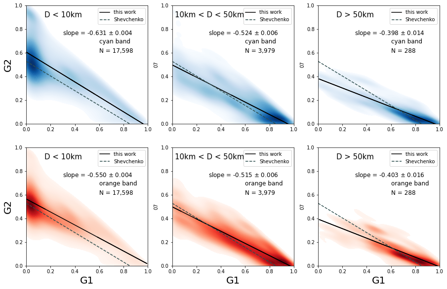
Figure 1: G1, G2-distributions for three diameter ranges of MB objects, from the ATLAS dual-band photometry asteroid phase curve catalog, observed in cyan (blue adjustment) and orange (red adjustment). The black line corresponds to the linear fit of the sample with the slop value shown, and the dashed line corresponds to the linear fit with the 93 MB of work [9], for comparison.
This size dependence on the G1 - G2 phase space is particularly true for smaller objects. As our NEOs are an even smaller population than the MB's, we cannot estimate the albedo of small objects from their phase curve parameters, as shown in Figure 2, from the distribution of our 105 NEOs in the G1 - G2 phase space. Obviously, a larger dataset of very small MB objects is needed to confirm whether the behavior mentioned above is specific to NEOs or to all very small bodies in the Solar System.
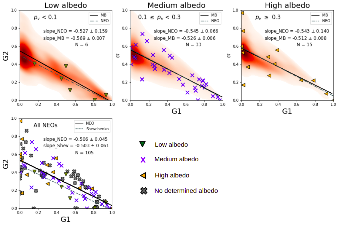
Figure 2 : G1, G2-pairs for MB 𝐷 < 10km with three albedo ranges for all NEOs with determined albedo (upper panels), and for all 105 NEO sample (bottom panel). The black line indicate the linear fits to the MB data and the dashed line indicate the linear fits to the NEO.
Acknowledgements
P.A., E.R., F.M., M.E, W.P. and J.M. would like to thank CNPq, FAPERJ and CAPES for their support through diverse fellowships. Support by CNPq (310964/2020-2) and FAPERJ (E-26/202.841/2017 and E-26/201.001/2021) is acknowledged by D.L. The authors are grateful to the IMPACTON team, in special to R. Souza, A. Santiago and J. Silva for the technical support.
References
[1] Bottke, W.F., Morbidelli, A., Jedicke, R., Petit, J.M., Levison, H.F., Michel, P., Metcalfe, T.S., 2002. . Icarus 156, 399–43.
[2] Morbidelli, A., Walsh, K.J., O’Brien, D.P., Minton, D.A., Bottke, W.F., 2015. pp. 493–507
[3] Helfenstein, P., Veverka, J., 1989. Asteroids II, University of Arizona Press, Tucson, pp. 557–593
[4] Rondón, E., Arcoverde, P., Monteiro, F., Medeiros, H., Navas, G., Lazzaro, D., Carvano, J.M., Rodrigues, T., 2019. 484, 2499–2513
[5] Rondón, E., Lazzaro, D., Carvano, J., Monteiro, F., Arcoverde, P., Evangelista, M., Michimani, J., Mesquita, W., Rodrigues, T., 2022. 372, 114723.
[6] Ieva, S., Arcoverde, P., Rondón, E., Giunta, A., Dotto, E., Lazzaro, D., Mazzotta Epifani, E., Perna, D., Fanasca, C., Rodrigues, T., Monteiro, F., Medeiros, H., Silva-Cabrera, J.S., Di Paola, A., 2022.
[7] Mahlke, M., Carry, B., Denneau, L., 2021. 354, 114094.
[8] Tonry, J.L., Denneau, L., Flewelling, H., Heinze, A.N., Onken, C.A., Smartt, S.J., Stalder, B., Weiland, H.J., Wolf, C., 2021. VizieR Online Data Catalog , J/ApJ/867/105.
[9] Shevchenko, V.G., Belskaya, I.N., Muinonen, K., Penttilä, A., Krugly, Y.N., Velichko, F.P., Chiorny, V.G., Slyusarev, I.G., Gaftonyuk, N.M., Tereschenko, I.A., 2016. . 123, 101–11
How to cite: Arcoverde, P., Rondón, E., Monteiro, F., Pereira, W., Ieva, S., Lazzaro, D., Michtchenko, T., Evangelista, M., Michimani, J., Mesquita, W., Corrêa, T., Dotto, E., Giunta, A., Di Paola, A., Medeiros, H., Carvano, J. M., and Rodrigues, T.: Physical properties of NEOs derived from their phase curves, Europlanet Science Congress 2022, Granada, Spain, 18–23 Sep 2022, EPSC2022-746, https://doi.org/10.5194/epsc2022-746, 2022.
Introduction
Asteroids lightcurves have been used extensively to derive many important physical characteristics such as rotational properties (rotational period and pole direction) and shape (Kaasalainen et al., 2004; Hanus et al., 2011; Durech et al., 2015), as well as to identify and characterize binary asteroids (Pravec et al., 2006). In addition, the rotational period and shape obtained from lightcurves can be used to estimate the internal cohesion strength required to prevent structural failure by centrifugal forces (e.g. Holsapple, 2007; Scheeres et al., 2010; Sánchez and Scheeres, 2014). Here, we will present some results of our extensive observational campaign for the physical characterization for a large sample of NEOs (Monteiro et al., 2017; Monteiro et al., 2018a,b; Rondón et al., 2019, 2020; Monteiro et al., 2020, 2021; Rondón et al., 2022; Monteiro et al., submitted).
Observations and data reduction
Photometric observations of about 150 NEOs were made at the Observatório Astronômico do Sertão de Itaparica (code Y28, OASI) of the IMPACTON project between 2012 and 2020. The images were acquired with the 1.0-m telescope using a 2048 x 2048 Apogee Alta U42 CCD camera. More details on the available instrumentation are given in Rondón et al., 2020. Lightcurve observations were carried out using sidereal tracking and an R-Johnson-Cousins filter. To obtain photometric spectra, observations were made using the g, r, i, z Sloan Digital Sky Survey (SDSS) filters. The science images were calibrated following the standard procedures, including bias, dark and flat-field images. The rotation periods were derived using a Fourier series analysis (Harris et al., 1989) while the spin direction and shape model were obtained by applying the lightcurve inversion method (Kaasalainen and Torppa, 2001; Kaasalainen et al., 2001). To investigate binary periods we used the "Dual Period Search" tool in MPO Canopus software. To obtain the photometric spectrum of some objetcs, we used standard field stars to calculate the zero-point of the night and, consequently, the calibrated magnitude of the asteroid.
Results
Reliable rotational periods and lightcurve amplitudes were determined for 88 NEOs (Monteiro et al. 2018a,b; Monteiro et al., submitted). For another 30 NEOs, only an estimate for the rotational period was obtained. The spin direction and shape model were obtained for about 15 NEOs. As an example, Fig. 1 shows the convex shape model for the NEO 2011 UW158, whose complete physical characterization was reported in Monteiro et al. (2020). These pole directions, along with those obtained from the DAMIT database (Durech et al. 2010), were used to analyze the pole distribution of the NEO population (Fig. 2). It is interesting to note that there appears to be a lack of poles toward the ecliptic plane. Clearly, a more representative sample is needed in order to derive robust conclusions.

Figure 1
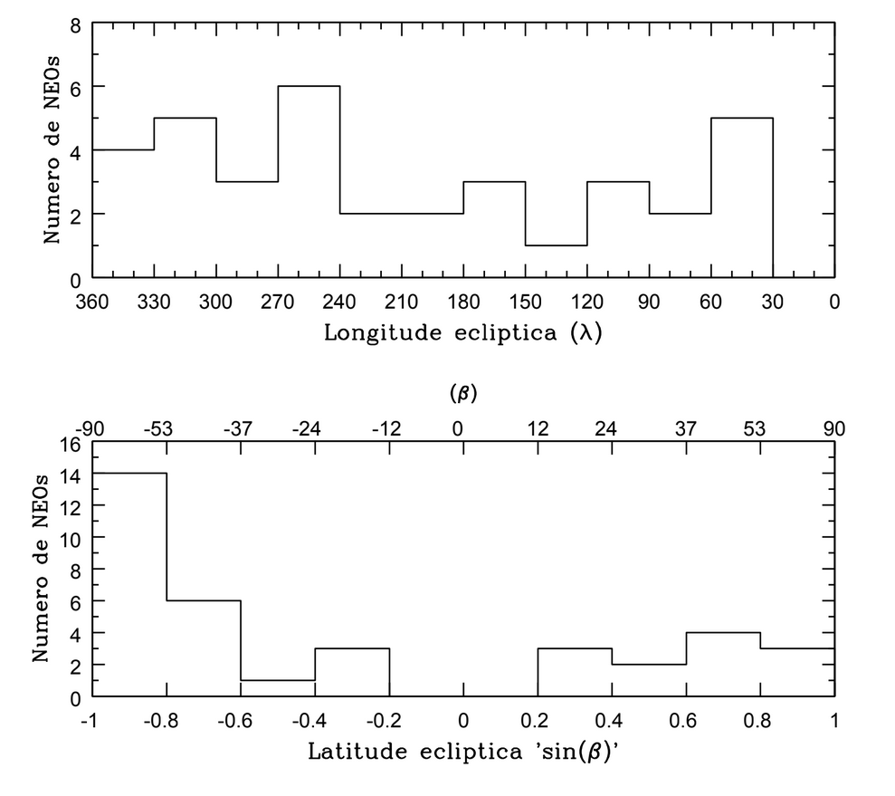
Figure 2
About 20 fast rotators in our sample were analyzed for signs of satellites. For 8 of them, binarity signatures were found in their lightcurves (Monteiro et al., submitted). Fig. 3 shows the primary and secondary lightcurves of a suspected binary showing a possible mutual observed event. For the possible binaries (138846) 2000 VJ61 and (243566) 1995 SA, we derived the minimum relative size of the components of 0.26 and 0.37, respectively. NEOs 2007 EX, 2014 KD91 and 2015 FS332 showed a secondary lightcurve, but no signs of eclipse/occultation, indicating the rotation of a possible satellite.
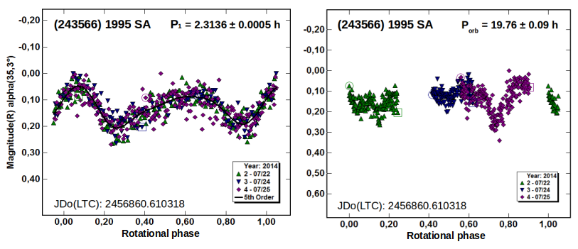
Figure 3
We found binarity signatures for 3 confirmed binaries (Monteiro et al., submitted). The NEO (31345) 1998 PG showed a secondary lightcurve, but no clear mutual events, with a period of about 16 h. The primary and secondary lightcurves of this objects is shown in Fig. 4. Finally, we estimate the internal cohesion strength required to prevent the failure of seventeen binary candidates that rotate beyond the cohesionless bodies limit. We found a minimum cohesion ranging from 3 to 90 Pa, which is in agreement with the numerical simulations reported in the literature (Sánchez and Scheeres, 2014). This analysis is included in detail in our recently submitted paper (Monteiro et al., submitted).
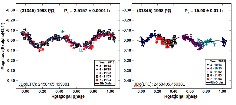
Figure 4
Conclusions
We determined a large sample of reliable lightcurves with well defined rotation period and amplitude. We derived the rotational period for about 30 PHAs and for some of them we indicated their possible taxonomic types. The derived spin direction, along with those obtained from the DAMIT database, continue to show a majority of retrograde rotators, which is consistent with a preferential transport route from the inner main belt. In addition, we identified 8 possible binary NEOs, which showed binarity signatures in their lightcurves. Finally, we showed that some fast rotators in our sample require an internal cohesion strength of 3 to 100 Pa to avoid structural failure by centrifugal forces.
Acknowledgements
F.M. thanks the financial support given by FAPERJ (E-26/201.877/2020). E.R., M.S., P.A, W.P., W.M., H.M. and T.C. would like to thank CAPES and CNPq for supporting this work through diverse fellowships. Support by CNPq (310964/2020-2) and FAPERJ (E-26/202.841/2017 and E-26/201.001/2021) is acknowledged by D.L. The authors are grateful to the IMPACTON team and, in particular, to R. Souza and A. Santiago for the technical support.
References
Durech J. et al. (2010), A&A, 513, A46.
Durech, J.,et al., 2015. Asteroids IV, pages 183-202.
Harris A. W., et al., 1989, Icarus, 77, 171.
Holsapple, K. A. (2007). Icarus, 187(2):500-509.
Kaasalainen, M. and Torppa, J. (2001). Icarus, 153:24-36.
Kaasalainen, M., Torppa, J., and Muinonen, K., 2001. Icarus, 153:37-51.
Kaasalainen, M., et al., 2004. Icarus, 167(1):178-196.
Margot J.L., et al., 2015. Asteroids IV. Pp 355–374.
Monteiro, F., et al., 2017. Minor Planet Bulletin 44, 20-22.
Monteiro, F., et al., 2018a. Minor Planet Bulletin 45, 221-224.
Monteiro, F., et al., 2018b. Planet. Space Sci. 164, 54-74.
Monteiro, F., et al., 2020. MNRAS, 495, 3990-4005.
Monteiro, F., et al., 2021. MNRAS 507, 5403–5414.
Perna, D., et al., 2016. AJ, 151(1):11.
Pravec, P., et al., 2006, icarus, 181, 63.
Rondón, E., et al., 2019. MNRAS, 484:2499–2513.
Rondón, E., et al., 2020. PASP, 132(1012):065001
Rondón, E., et al., 2022. Icarus 372, 114723.
Sánchez, P. and Scheeres, D. J., 2014. Meteoritics and Planetary Science, 49(5):788-811.
Scheeres, D. J., et al., 2010. Icarus, 210(2):968-984.
How to cite: Monteiro, F., Lazzaro, D., Rondón, E., Evangelista-Santana, M., Arcoverde, P., Pereira, W., Mesquita, W., Michimani, J., Medeiros, H., Corrêa, T., Silva-Cabrera, J., and Rodrigues, T.: Physical characterization of near-Earth objects from the IMPACTON project, Europlanet Science Congress 2022, Granada, Spain, 18–23 Sep 2022, EPSC2022-767, https://doi.org/10.5194/epsc2022-767, 2022.
Introduction
Asteroid (594913) 'Aylo'chaxnim, formerly designated as 2020 AV2, is the only one known to orbit inside Venus orbit. It was first observed by the Zwicky Transient Facility on January 4, 2020 (Bolin et al. 2020) and it may represent the largest member of a new population of small bodies with the aphelion distance smaller than 0.718 a.u., called Vatiras (Greenstreet et al. 2012). Because of its orbit, the surface of this asteroid is being constantly modified by the high temperature, by the strong solar wind irradiation that characterizes the innermost region of the Solar system, and by high-energy micrometeorite impacts. Thus, it represents an extreme case when compared with the near-Earth asteroids.
Based on the observations obtained on January 13, and 14, 2020, we found that 'Aylo'chaxnim has a wide spectral absorption band around 1 μm that represents the signature of an olivine-rich composition. The estimated absorption band center BIC = 1.08 ± 0.02 μm corresponds to a ferroan olivine mineralogy (Popescu et al. 2020 MNRAS). By comparing these spectra with the taxonomic types from Bus-DeMeo taxonomy, we found Sa types as the best fit for the (0.5 - 1.5 ) μm spectral interval. The classification as an S-complex asteroid was also reported by Bolin et al. (2020 EPSC) based on a visible spectrum obtained on January 23, 2020 with the Keck I telescope. They also reported a reddish surface with g-r=0.65 mag and r – i = 0.23 mag and i-z = 0.11 mag.
Here we report new near-infrared spectra, in the range 0.8-2.5 μm, obtained using the 3m NASA Infrared Telescope Facility (NASA IRTF). The observations were performed during August 2021, when the object was close to its maximum solar elongation of 40 deg.
Table 1. Observational circumstances for (594913) 'Aylo'chaxnim.
|
Spec. ID |
Average UT |
Average airmass |
Total exp.[sec] |
No. of exp. |
|
S1 |
2021-08-11T14:38:38 |
2.8 |
1912.7 |
16 x 120 sec |
|
S2 |
2021-08-12T14:37:21 |
2.9 |
1793.2 |
15 x 120 sec |
|
S3 |
2021-08-14T15:05:12 |
2.3 |
836.8 |
7 x 120 sec |
Observations
We used the SpeX instrument, with the PRISM mode and a slit of 0.8 x 15 arcsec. This configuration allowed us to cover the 0.82 – 2.5 μm spectral interval. The spectral images were acquired in the ABBA mode. Table 1 shows the observation log for the three sets of data. The object was observable at an air-mass of ~2.5-3 for about 30 min before the start of the morning twilight. We noticed a wide apparent magnitude variation between the nights.
In order to obtain the reflectance spectrum, the asteroid’s observed spectral data must be divided by that of a solar analog. We could observe only one solar analog, a G2V star, namely GSC 01881-01236, which was the best suited for our work in terms of apparent vicinity and time constraints. The data reduction was performed with the Spextool package (Cushing et al. 2004).
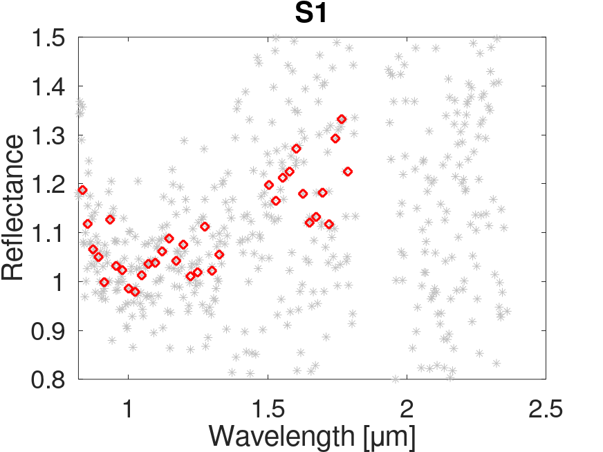
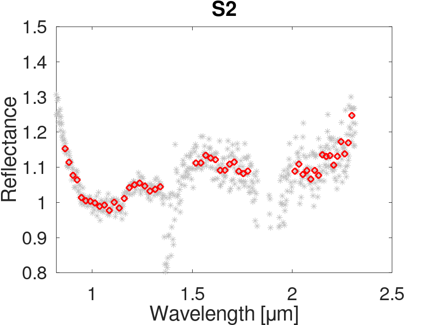
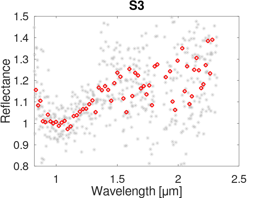
Fig.1 The spectral data obtained with IRTF/SpeX during August 2021 for (594913) 'Aylo'chaxnim. The gray points represent the data obtained as provided by Spextool (the pipeline used to reduce the spectral images). The red points were obtained by binning every 9 points from the original data (the gray ones). The observational details associated with S1, S2, S3 are described in Table 1. The data are normalized at 1 μm.
Results
The spectra obtained during the three nights are identical up to 1.3 μm. They also match the spectrum obtained in 2020 (Fig. 2). The S1 and S3 spectra are redder compared with S2, for wavelengths longer than 1.3 μm. A thermal tail is identifiable for S2.
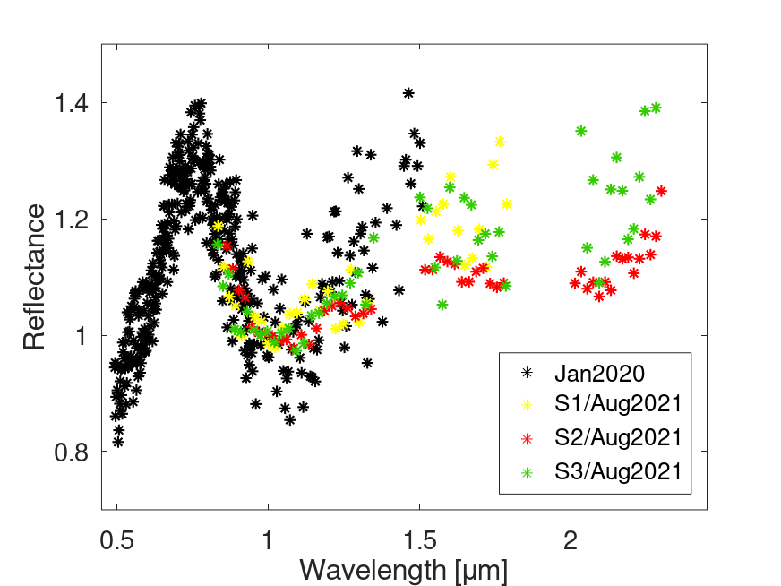
Fig. 2 Comparison between the spectra obtained during January 2020 (Popescu et al. 2020), and those obtained during August 2021. All spectra are normalized to 1 μm.
The absorption band minima (BImin) is located at 1.07 +/- 0.015 μm for S2, and 1.09 +/-0.02 μm for S3 (we did not compute this band center for S1 due to its large error-bars). This result is consistent with the olivine rich composition proposed based on the 2020 observations. The S2, which has the best signal to noise ratio, shows a possible feature at 1.25-1.30 μm, which can also be attributed to olivine.
We used the S2 spectrum for comparison with the RELAB spectral database . Its shape is best matched by the CK meteorites (Cloutis et al. 2021). These are characterized by an olivine associated absorption band in the 1.05 μm region. Compared to pure olivine, CK spectra are darker, have a more subdued olivine absorption band, and are often more blue-sloped (Cloutis et al. 2012).
References
1. Bolin et al. 2020 , Minor Planet Electronic Circ., No. 2020-A99 (2020)
2. Bolin et al. 2020, the 14th Europlanet Science Congress 2020, abstract id. EPSC2020-482
3. Cloutis et al. 2012, Icarus, Volume 221, Issue 2, p. 911-924
4. Greenstreet S., Ngo H., Gladman B., 2012, Icarus, 217, 355
5. Popescu et al. 2020, MNRAS, Volume 496, Issue 3, pp. 3572-3581
Acknowledgments
The work of MP was supported by a grant of the Romanian National Authority for Scientific Research – UEFISCDI, project number PN-III-P1-1.1- TE-2019-1504. The work of MP, JdL, JL, is made in the framework of EU-funded project ”NEOROCKS - The NEO Rapid Observation, Characterization and Key Simulations project”, SU-SPACE-23-SEC-2019 from the Horizon 2020 - Work Programme 2018-2020, under grant agreement No 870403. The abstract make use of data published by the Relab Spectral Database
How to cite: Popescu, M., de la Fuente Marcos, C., Văduvescu, O., de la Fuente Marcos, R., Bus, S., de León, J., Licandro, J., Tatsumi, E., and Simion, G. N.: New near-infrared spectra of (594913) 'Aylo'chaxnim, the first known asteroid orbiting inside Venus orbit, Europlanet Science Congress 2022, Granada, Spain, 18–23 Sep 2022, EPSC2022-804, https://doi.org/10.5194/epsc2022-804, 2022.
Introduction
The asteroid (4660) Nereus is considered one of the most accessible targets for a rendez-vous space mission. It was proposed as a possible target for the NASA Near-Earth Asteroid Rendezvous (NEAR) and for JAXA Hayabusa spacecraft.
The lightcurve analysis and the radar shape modeling revealed a long rotational period of ≅ 15.16 ± 0.04 h [1, 2]. The radar [2] and thermal [3] observations report optical albedo values of 0.54 (-0.09, +0.03) and 0.55 ± 0.17 respectively. Coupled with the featureless spectrum [4], Nereus is classified as an E-type object in the Tholen taxonomy. This class has been associated with enstatite achondrite meteorites.
During the fall of 2020 and the beginning of 2021, (4660) Nereus made a favorable apparition for observations with ground-based telescopes. It had an apparent magnitude brighter than 18.5 V mag. for about 7 months. The peak brightness was 12.9 on the night of December 7. In this context, we performed an extended characterization using various telescopes. Thus, we report light-curves, spectro-photometric data and spectral observations for Nereus.
Observations
We obtain the light curve of (4660) Nereus using the T025-BD4SB, a 0.25 m aperture telescope located at the Bucharest Astronomical Institute , Romania. About 65 hours of observations were obtained during 8 nights spread between October 27 and November 25, 2021. These data were acquired using the QHY294M CMOS camera.
The color indices in the visible region were determined using the MuSCAT2 instrument of the 1.52 m Telescopio Carlos Sanchez (TCS) located in Tenerife, Spain. This instrument allows simultaneous images with the broad band filters g (0.40 - 0.55 μm), r (0.550 - 0.70 μm), i (0.70 - 0.82 μm), and zs (0.82 - 0.92 μm). As such, we gathered 15.2 hours of data during six nights of observations spread over October 02, 2021 until April 02, 2022.
Additional photometry data was obtained using the 2.54 m Isaac Newton Telescope (La Palma, Spain) equipped with Wide Field Camera (WFC). We obtained 6 hrs of photometric observations using the B, V, R Johnson filters, and the r and z SDSS filters during the nights of March 2, and April 18, 2022.
The spectrum in the near-infrared region was obtained using the 3.58m Galileo National Telescope (La Palma, Spain). We used the near-infrared camera spectrometer (NICS) with the AMICI prism and a a.5 arcsec slit-width. The configuration allowed a resolving power of R=50 and a spectral interval coverage of 0.8 - 2.45 μm.
The photometric data reduction has been made using the Photometry Pipeline [5]. We also used IRAF and MP0 Canopus to cross-check the results. The spectral data was reduced using a dedicated pipeline written in Python.
Results
First we performed a photometric analysis of the asteroid (4660) Nereus. We determined its period using the Lomb-Scargle Periodogram and we investigated the YORP effect on the asteroid. Subsequently, we obtained the object's phase curve and we computed its absolute magnitude (H) and the slope parameter (G). Then we determined its color indices and we used them for classification. Finally, we reviewed its taxonomic classification based on the new acquired spectrum.
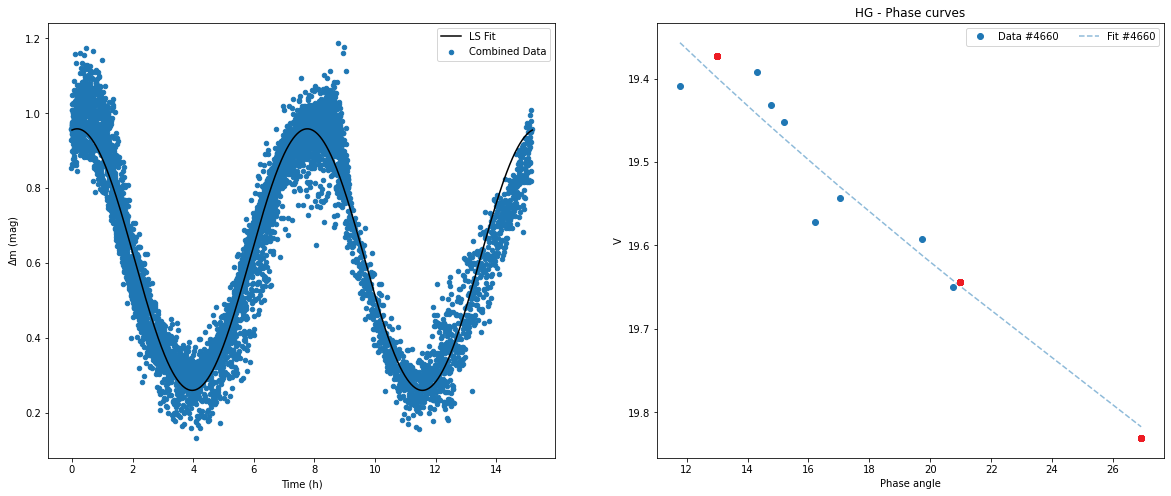
Fig 1: Left: The folded lightcurve of (4660) Nereus obtained by combining
the data from T025-BD4SB and TCS. Right: Phase curve of (4660) Nereus. The
red points are TCS observations while the blue ones are T025-BD4SB. The
dotted line represents the H-G model fit.
The Lomb-Scargle periodogram peaks at a value of 15.19 hrs. The light-curve corresponding to this period is plotted in Fig. 1. This value is in the range reported by [1] determined a period of 15.1 ± 1.2 h. It is also compatible with the value obtained using radar data [2] of 15.16 ± 0.04 h.
Because of its size, (4660) Nereus is subjected to the YORP effect which affects the asteroid's spin rate. We estimate a change of one to four seconds for its rotation period in a range of 10 years. Unfortunately, the previous values for its rotation period have much larger uncertainties. As such, another favorable observing window is needed to quantify this effect.
Furthermore, we determine the phase curve of the asteroid in order to obtain its absolute magnitude. In order to do this, we use the Pyedra software [6]. The algorithm allowed us to use the H-G model [7] in order to fit our phase curve (Fig. 1). We obtained the absolute magnitude (H = 18.69 ± 0.18) and the slope parameter (G = 0.209 ± 0.06). In Fig. 1 we show our results. For comparison, [8] reported a value of 18.58 ± 0.06.
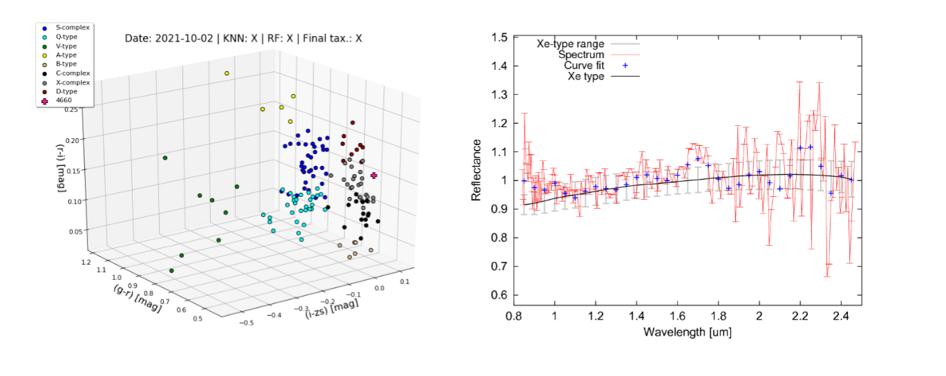
Fig 2: Left: The color-color diagram of (4660) Nereus compared with the reference data-set (Popescu et al. 2022 - paper in preparation). Right: The near-infrared spectrum of (4660) Nereus and its taxonomic classification.
The TCS/MuSCAT2 instrument allowed us to simultaneously obtain the light-curve in all four filters. We found (g-r) = 0.537 ± 0.048, (r-i) = 0.145 ± 0.012, (i-zs) = 0.091 ± 0.017. In addition to these values, we obtained the (B-R) = 1.15 ± 0.05 mag, and ± = 0.043 ± 0.03 mag color indices.
The average color values obtained with TCS/MuSCAT2 are compatible with an X-complex classification (Fig. 2). This result complements the spectral classification based on the data obtained with TNG/NICs instrument. The spectrum shown in Fig. 2 is compatible with the Xe type.
Acknowledgments
The work of MP and RMG was supported by a grant of the Romanian National Authority for Scientific Research -- UEFISCDI, project number PN-III-P1-1.1-TE-2019-1504. The work of MP, JdL, JL, and DM is made in the framework of EU-funded project "NEOROCKS project", SU-SPACE-23-SEC-2019 from the Horizon 2020 - Work Programme 2018-2020. The observations were obtained trough the EURONEAR collaboration.
[1] Y. Ishibashi et al, 2000, Earth, Planets and Space
[2] Marina Brozovic et al, 2009, Icarus
[3] Marco Delb ́o et al, 2003, Icarus
[4] Richard P. Binzel et al, 2004, Asteroids II
[5] M. Mommert, 2017, Astronomy and Computing
[6] M. Colazo et al, 2022, Astronomy and Computing
[7] Edward Bowell et al, 1989, Asteroids II
[8] Y. Ishibashi et al, 2000, Advances in Space Research
How to cite: Mansour, J. A., Popescu, M., de León, J., Berteșteanu, D., Morate, D., Văduvescu, O., Licandro, J., Dumitru, B. A., Simion, G. N., Gherase, R. M., Pinter, V., and Tatsumi, E.: Physical characterization of asteroid (4660) Nereus, Europlanet Science Congress 2022, Granada, Spain, 18–23 Sep 2022, EPSC2022-984, https://doi.org/10.5194/epsc2022-984, 2022.
Introduction
When talking about Trojan asteroids -- bodies orbiting around the L4 or L5 Lagrangian points of a Sun-planet system -- it is inevitable to refer to Jupiter. This giant planet has, by far, the largest reservoir of Trojan asteroids with thousands of objects discovered since 1906. We currently know, however, that other planets are also able to host asteroids in such a peculiar orbital configuration, although in much smaller number. Trojan asteroids can be important to study the formation and evolution of our Solar System since, some of them – called primordials -- might be remnants of the formation processes of the hosting planet. The first Earth Trojan asteroid (ETA) was discovered in 2010 librating around L4. Thenceforth, several dedicated observational campaigns have been scrutinizing L4 and L5 areas, trying to find a second ETA. In this work we describe how we confirmed (614689) 2020 XL5 as the second ETA and we discuss why it is so arduous to detect these objects with groundbased observations.
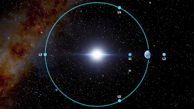
Fig.1: The Sun-Earth Lagrangian points. 2020 XL5 is librating around L4. (NOIRLab/NSF/AURA/J. da Silva)
Observations
Asteroid 2020 XL5 was discovered by the Pan-STARRS1 survey on 2020 December 12. An initial orbit determination was obtained from follow-up observations gathered during the next few weeks. Some solutions suggested that 2020 XL5’s orbit could be librating around L4, but the short arc covered with observations was still to short for a long term analysis [8]. However, observations were challenging due to the object’s faintness (V~22 mag) and its proximity with the Sun (ε<40°).
Our team started a follow-up campaign and was able to obtain a few new measurements (Fig.2) of the object during February and March 2021 using ESA’s Optical Ground Station (OGS) 1.0 m telescope, the 4.1 m Southern Astrophysical Research (SOAR) telescope and the 4.3 m Lowell Discovery Telescope (LDT). Despite the successful results of the observation campaign and the consequent improvement of the orbit of 2020 XL5, the arc was still too short for a conclusive result. However, the orbit now allowed us for a detective work among the tons of data from the surveys. Precoveries were found in the files of the Catalina Sky Survey (1.5 m Mt. Lemmon telescope), DECam instrument (4.1 m Victor M. Blanco telescope) and the archive of the 1.8 m Pan-STARRS survey (Fig. 3).
Fig.2: LDT detection of 2020 XL5.
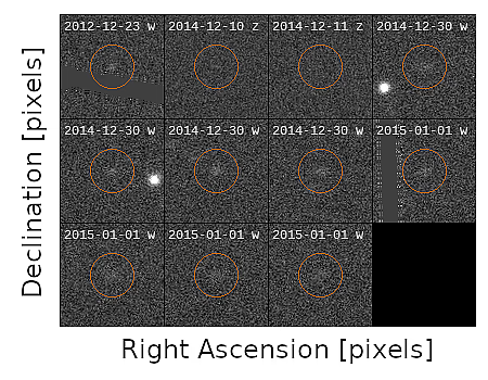
Fig.3: Pan-STARRS ancillary data of 2020 XL5.
Results
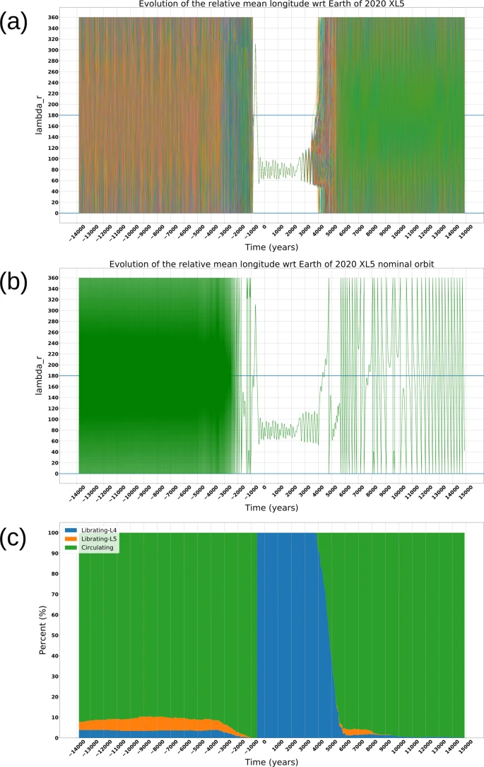
Fig.4: a The relative mean longitude (λr) evolution of the 2020 XL5 nominal orbit and clones orbit over 29 000 years, where each clone orbit is represented by a different color, while the green line represents the nominal orbit. b Evolution of λr for the nominal orbit of 2020 XL5. c Stack plot representing the behavior of the nominal orbit and the 800 clone orbits. In the plot the time t0 = 0 is the mean epoch of the orbits.
With all the data in hand, we generated hundreds of clone orbits along a time span of 29 000 years, applying the Cholesky method for multivariate normal distributions [9]. The study of the relative mean longitude of 2020 XL5 (Fig.4) revealed that the object is indeed a transient ETA, which was captured some 500 years ago and will keep librating around L4 for at least 4000 more years. In addition, we performed a preliminar physical characterization of the asteroid by means of photometry. We estimated its absolute magnitude to be Hr =18.58 (+0.16−0.15), and color indices suggestive of a C-complex taxonomy. Assuming an albedo of 0.06 ± 0.03 we obtained a bulk diameter of 1.18 ± 0.08 km.
References
[1] Dvorak, R. & Schwarz, R. On the stability regions of the Trojan asteroids. Celest. Mech. Dyn. Astron. 92, 19–28 (2005).
[2] Connors, M., Wiegert, P. & Veillet, C. Earth’s Trojan asteroid. Nature 475, 481–483 (2011).
[3] Wiegert, P. A., Innanen, K. A. & Mikkola, S. An asteroidal companion to the Earth. Nature 387, 685–686 (1997).
[4] Whiteley, R. J. & Tholen, D. J. A CCD search for Lagrangian asteroids of the Earth-Sun system. Icarus 136, 154–167 (1998).
[5] Markwardt, L. et al. Search for L5 Earth Trojans with DECam. Mon. Not. R. Astron. Soc. 492, 6105–6119 (2020).
[6] Lifset, N., Golovich, N., Green, E., Armstrong, R. & Yeager, T. A search for L4 Earth Trojan asteroids using a novel track-before-detect multiepoch pipeline. Astron. J. 161, 282 (2021).
[7] Santana-Ros et al. Orbital stability analysis and photometric characterization of the second Earth Trojan asteroid 2020 XL5. Nature Communications 13, 447 (2022)
[8] de la Fuente Marcos, C. & de la Fuente Marcos, R. Transient terrestrial Trojans: comparative short-term dynamical evolution of 2010 TK7 and 2020 XL5. Res. Notes Am. Astronomical Soc. 5, 29 (2021).
[9] T., T. N. Essentials of Monte Carlo Simulation (Springer-Verlag, New York, 2013).
Acknowledgements
TSR acknowledges funding from the NEO-MAPP project (H2020-EU-2-1-6/870377). This work was (partially) funded by the Spanish MICIN/AEI/10.13039/ the Institute of Cosmos Sciences University of Barcelona (ICCUB, Unidad de Excelencia ‘María de Maeztu’) through grant CEX2019-000918-M.
How to cite: Santana-Ros, T., Micheli, M., Faggioli, L., Cennamo, R., Devogèle, M., Alvarez-Candal, A., Liu, P.-Y., Benavidez, P. G., and Campo Bagatin, A.: Operating manual on how to find an Earth Trojan asteroid, Europlanet Science Congress 2022, Granada, Spain, 18–23 Sep 2022, EPSC2022-986, https://doi.org/10.5194/epsc2022-986, 2022.
The Herschel Space Observatory observed with its PACS and SPIRE instruments a diverse selection of astronomical objects, including Solar System objects (SSOs), either in dedicated measurements or serendipitously. The infrared observations of asteroids helped scientists to determine their physical and thermal properties. In addition, PACS and SPIRE observations of selected large asteroids were used for a wide range of calibration aspects. Due to their strong thermal emission, SSOs may sporadically also contaminate the photometric measurements of other sources. Racero et al. (2022) presented ESASky tools to find these moving targets in Herschel data products. As a first step, we focused on the flux extraction of these serendipitous observations of SSOs in Herschel/PACS measurements at 70, 100 and 160 μm. We obtain far-infrared photometry on the PACS maps, either by extracting the flux densities from the existing standard data products, or via re-reducing the PACS maps in the co-moving frame of the target. Based on these scientifically very important far-IR flux densities, in combination with already published IR detections (Szak ́ats et al., 2020), we perform radiometric studies to determine the objects’ physical and thermal properties with unprecedented accuracy.
A natural continuation of our current work is the extension to SPIRE maps at 250, 350, and 500 μm, with a two-fold aim. First, to find serendipitous asteroids, extract new submm flux densities and flag sources in the SPIRE Point Source Catalog (Schulz et al., 2018) for possible contamination. In addition, the dedicated SPIRE observations of asteroids for various calibration activities are not yet published. As the SPIRE absolute photometry is connected to planet models, these asteroid flux densities are of great value and will put strong constraints on their submm emissivity properties. All SPIRE asteroid measurements were reprocessed and calibrated with the latest pipeline. The final maps are then used to extract high quality IR/submm flux densities. The flux densities are then added to the publicly available SBNAF Infrared Database (Szakáts et al., 2020).
We collected the Herschel/SPIRE targeted asteroid measurements, and we went through the list of SPIRE observations with potential serendipitous asteroid detections (from Racero et al. 2022). We only considered those, where the isvisible flag was ’true’. In a first step we verified that the photometry via the point source calibrated maps and the SSO calibrated maps are in agreement. This is important because all the dedicated measurements were reprocessed in the object co-moving frame and made available in the Herschel Science Archive, but not the serendipitous ones. Our tests confirmed that the two maps give the same flux densities within the error bars, so there is no need to reprocess the serendipitous maps into the co-moving frame. In a second part of the project, after making all flux densities available in the IR database, we perform radiometric
studies for individual asteroids. Depending on the a priori knowledge for a given object, we distinguish between the following five categories: (1) mission targets, well-known/-studied objects; (2) objects with good-quality spin-shape solution and multi-epoch/-mission thermal measurements; (3) good-quality spin-shape solution, but very limited or no thermal measurements available; (4) no good-quality spin-shape solution, but sufficient multi-epoch/-mission thermal measurements available; (5)
no spin-shape solution and very limited thermal measurements available. In each of these five categories, the SPIRE (and PACS) flux densities are important to obtain the object’s emissivity properties, to constrain the thermal properties of the surface or to establish basic radiometric size-albedo solutions.
We will present an overview of the new far-IR and sub-mm measurements (for about 17 dedicated program asteroids and several different main-belt asteroids), the extracted flux densities, and applications for the different categories.
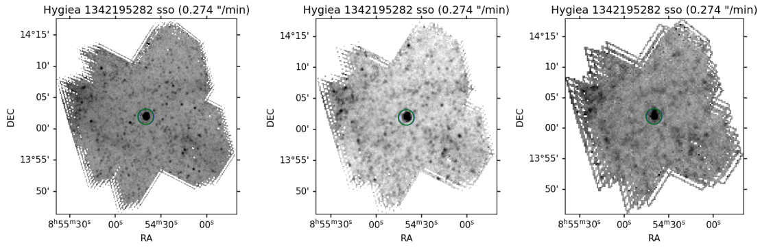
Figure 1: The SPIRE maps for asteroid (10) Hygiea at 250, 350, and 500 μm, taken from a dedicated calibration sequence, and processed in the object’s co-moving frame.
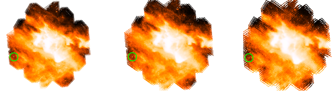
Figure 2: The SPIRE maps of the serendipitously seen asteroid (464) Megaira (marked by the green circles) at 250, 350, and 500 μm.
How to cite: Szakáts, R., Kiss, C., Müller, T., and Valtchanov, I.: Herschel/SPIRE photometry of targeted and serendipitously observed asteroids, Europlanet Science Congress 2022, Granada, Spain, 18–23 Sep 2022, EPSC2022-1060, https://doi.org/10.5194/epsc2022-1060, 2022.
Introduction
2022 AB is a very small near-Earth asteroid that passed Earth at a distance of 9.6 lunar distances on 20 January.
Our campaign started on 4 January and until 26 January, we observed 2022 AB using telescopes located in many places around the world. More about the campaign, including the determination of the phase curve, will be presented during this conference in a separate presentation [2]. Here we only present results regarding the colour indices, taxonomic class, and diameter. We organised a similar observation campaign for 2021 DW1 in 2021 [3][4][5].
Rotation period
In determining the colours indices, it is very important to know the rotation period of the asteroid. We discussed the issues, especially in the field of NEAs, at the conference last year [5].
We briefly discuss the determination of the rotation period using an example of observations from the first night of the campaign of 2022 AB. More will be discussed in [2].
We used a 0.7-m RBT/PST2 telescope(Arizona), 5-s exposures, and the clear filter. We observed object for 1.5 hours and we create composite lightcurve with Fourier series fit (see Figure 1). In this way, we determined the rotation period P=182 s.
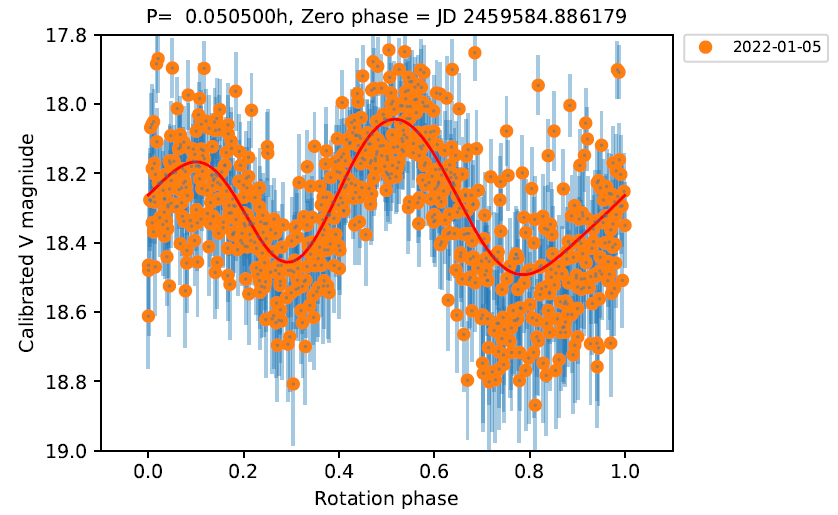
Figure 1: Example of composite lightcurve of 2022 AB.
Colour indices
The preliminary results presented here are based on most of the data obtained. The full results will be presented during the conference.
To determine the colour indices, we used observations from three telescopes: 0.7-m RBT, 1-m telescope of DOAO (South Korea), and 1-m telescope of Pic du Midi Observatory (France). Telescopes from DOAO and Pic du Midi observed the asteroid with an exposure time of several seconds in the B,V,R,I (DOAO) or g’,r’,i’,z’ (Pic du Midi) filters. Due to changes in the geometry of the observations, we divided the observations into several sets. Using solar analogues, we transformed the brightness in B,V,R,I into g’,r’,i’,z’ bands, respectively. Then, knowing the rotation period, we composited the lightcurves to determine the shifts between the lightcurves in the given bands. We have prepared the composited lightcurves separately for each set. An example is shown in Figure 2. RBT observations were made in B,V,R filters and, as we mentioned, transformed them into g’,r’,i’. In this case, we used knowledge of the rotation period to average the brightness measurements over the period, exposure time Texp=P=182s. Adjacent measurements in different bands allowed us to determine a series of colour indices that we averaged as one set. The results for each set are shown in Table 1.
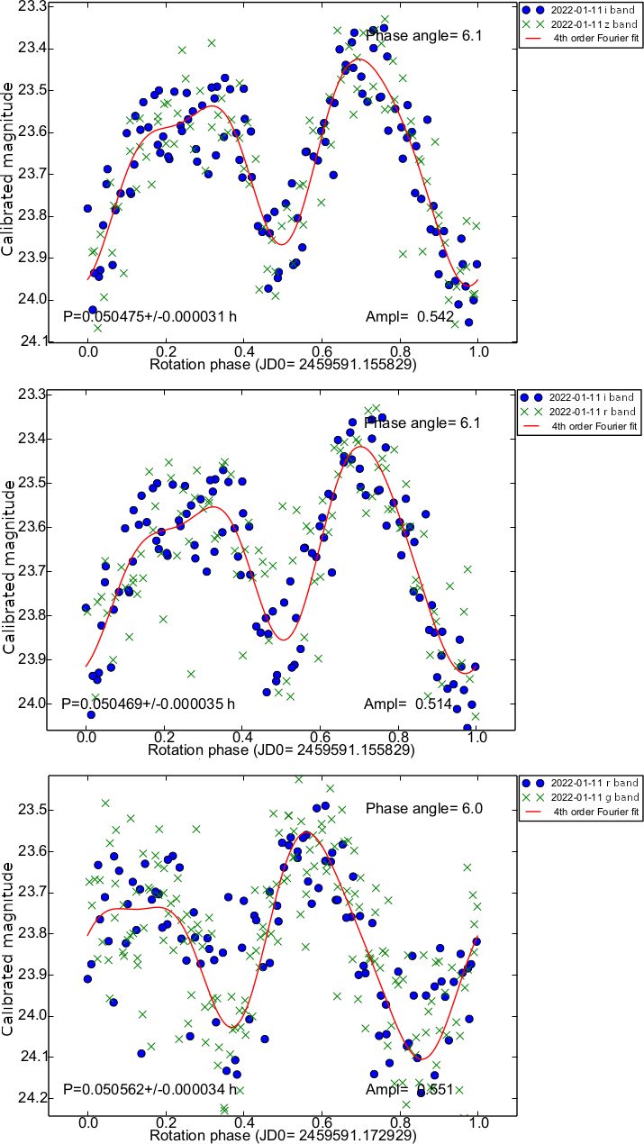
Figure 2: Composite lightcurves for DOAO set 1. Top: lightcurves in i’ (dots) and z’ band (crosses), middle: i’ and (dots) and r’ (crosses) bands, bottom: r’ (dots) and g’ (cross) bands.

Table 1: Preliminary results of colour indices for each set.
Taxonomy
To determine the taxonomic class of 2022 AB, we converted the average value of colour indices to the reflection coefficients Rr,Ri and Rz, normalised to the reflection values in the g band, using the formula [6]:
Rf=10−0.4[(f−g)−(f☉−g☉)]
Next, we compared them with spectra of different taxonomic classes, as given by [6]. In Figure 3 we present the reflective value of the asteroid compared to similar taxonomic classes. B class asteroids are rare and they are mainly associated with the outer main belt. 2022 AB as an NEA is an unlikely class B asteroid. The Cb class fits well with the data of 2022 AB and is the only one to show the common with 2022 AB characteristic of visible absorption around 0.6 micrometre. We suggest that 2022 AB is most likely a type Cb asteroid.

Figure 3: Plot of reflectivities values of B,Cb,Ch asteroid classes (black dots) and 2022 AB (red dots). Data for the B,Cb, and Ch classes were taken from [6].
Diameter
We can determine the diameter knowing the absolute magnitude H and the albedo pV according to equation [7]:
Deff=1329×10−H/5×pV−0.5
At the conference, we will present the results based on the determined H from the phase curve, but for now we used the approximate H=23.6±0.36 given by JPL[1]. Albedo for Cb class asteroids: pV=0.059±0.027 [8], hence Deff=0.104±0.029 km.

Figure 4: Rotation period-diameter plot. The red dotted line is the spin barrier (2.2 h). Other asteroid data come from LCDB [8].
Acknowledgements
This research was funded in whole or in part by the National Science Centre, Poland, grant No. 2021/41/N/ST9/04259.
References
[1] https://ssd.jpl.nasa.gov
[2] Kwiatkowski et al. (2022) Photometry and model of near-Earth asteroid 2022 AB from one apparition,EPSC 2022, held 18–23 September 2022 in Granada, Spain
[3] Kwiatkowski et al. (2021) A&A 656, A126
[4] Kwiatkowski et al. (2021) Photometry and model of near-Earth asteroid 2021 DW1 from one apparition, EPSC 2021, held virtually, 13-24 September 2021
[5] Koleńczuk et al. (2021) Determination of colour indices of super-fast rotator near-Earth asteroids, EPSC 2021, held virtually, 13-24 September 2021
[6] DeMeo & Carry (2013), Icarus 226, 723
[7] Fowler and Chillemi (1992) Phillips Laboratory, Hanscom AF Base, MA, 17–43
[8] Warner et al. (2009) Icarus 202, 134
How to cite: Koleńczuk, P., Kwiatkowski, T., Kamińska, M., Kamiński, K., Colas, F., Klotz, A., Kim, T., and Birlan, M.: Colours and taxonomy of 2022 AB: a super fast rotating near-Earth asteroid, Europlanet Science Congress 2022, Granada, Spain, 18–23 Sep 2022, EPSC2022-1161, https://doi.org/10.5194/epsc2022-1161, 2022.
There are a large number of small bodies (known as trans-Neptunian objects or TNOs) in the outer solar system that show different types of dynamical behavior. These objects can be considered as "probes" of the dynamical and chemical history of the Solar System. These asteroids or planetezimals are relics of dynamical events among and beyond the giant planets, and the current observed orbital distribution of the TNOs is a sign of large-scale changes in the position of the giant planets. The dynamical classification of the bodies of this outer region of the Solar System helps to understand the structure and formation of the Solar System. In this work, we performed a comprehensive survey on the TNOs. By using the FAIR method considering all known small bodies in outer Solar System (more than 4,000 asteroids classified as TNO in the JPL database), we identified several MMRs between these bodies and the planet Neptune. According to our dynamical investigations, there are two types of resonant behaviour of asteroids; namely, when the critical argument (resonance variable) shows short-term or long-term libration.
How to cite: Forgács-Dajka, E., Kővári, E., Kovács, T., Kiss, C., and Sándor, Z.: Dynamical Investigation of Trans-Neptunian Objects in particular the Mean-Motion Resonances with Neptune, Europlanet Science Congress 2022, Granada, Spain, 18–23 Sep 2022, EPSC2022-1213, https://doi.org/10.5194/epsc2022-1213, 2022.
In a recent research, we carried out a large-scale survey of the trans-Neptunian objects (TNOs) by means of dynamical maps. We identified the most important MMRs and explored their dynamical role through the quantification of the chaotic diffusion and that of the stability times of the small bodies. The chaotic diffusion is of fundamental importance for its rate determines the long-term evolution of a given celestial system. To estimate the rate of the diffusion (that is, to compute the diffusion coefficients) in the case of more than 4100 TNOs, we initiated the use of the Shannon entropy. This latter quantity allows, on the one hand, to measure the extent of unstable regions in the phase space (and thus serves as an indicator of chaos), and also enables the direct measurement of the diffusion coefficients. The characteristic times of stability - in the case of normal diffusion - are then achieved by taking the inverse of the diffusion coefficients. In the knowledge of the chaotic diffusion and stability times for as large a TNO sample as the one indicated above, the overall structure of the trans-Neptunian space can be mapped, along with the specification of dynamical classes or the update of the existing ones.
How to cite: Kővári, E., Forgács-Dajka, E., Kovács, T., Kiss, C., and Sándor, Z.: Chaotic behaviours of different time-scales in the trans-Neptunian space, Europlanet Science Congress 2022, Granada, Spain, 18–23 Sep 2022, EPSC2022-1216, https://doi.org/10.5194/epsc2022-1216, 2022.
SB2 | Small bodies from the active Main Belt to the Oort cloud and beyond
Comets are thought to have preserved dust particles from the very beginning of Solar System formation, providing a unique insight into intricate processes like dust growth mechanisms. The Rosetta mission offered the best opportunity to investigate nearly pristine cometary dust particles of comet 67P/Churyumov–Gerasimenko. In particular, among the three in-situ dust instruments, the MIDAS (Micro-Imaging Dust Analysis System) atomic force microscope collected cometary dust particles with sizes from hundreds of nanometres to tens of micrometres on dedicated targets and recorded their 3D topographic information and related parameters (Bentley et al. 2016a). However, the straightforward dust collection strategy, i.e., simply hitting the collection targets, leads to an unknown degree of collection alteration (Mannel et al. 2016; Bentley et al. 2016b).
We aim to understand dust alteration during collection and determine which structural properties of the MIDAS dust particle remained pristine. An exhaustive dust particle catalogue for MIDAS is created, containing 3494 dust particles with (meta)data. Among these particles, we carefully select 1082 particles that are eligible for a more extensive structural investigation. First, we generate sophisticated dust maps showing the distribution of the selected dust particles on the collection targets and investigate dust clustering, i.e., determination of which of the particles stem from a single parent particle that fragmented upon the collection impact. Additionally, in the collaboration with Longobardo et al. in preparation, we use an algorithm to determine from which cometary source regions which MIDAS particles were stemming (Longobardo et al. 2020). Next, we develop MIDAS particle shape descriptors such as aspect ratio (i.e., height of the particle divided by the square root of area; Lasue et al. 2019), elongation, circularity, convexity, and particle surface/volume distribution. Furthermore, we compare the structure of the MIDAS dust particles and the clusters to those found in the laboratory experiments (Ellerborek et al. 2017) and by COSIMA/Rosetta (Langevin et al. 2016). Finally, we combine our findings to calculate a pristinity score for MIDAS particles and determine the most pristine particles and their properties.
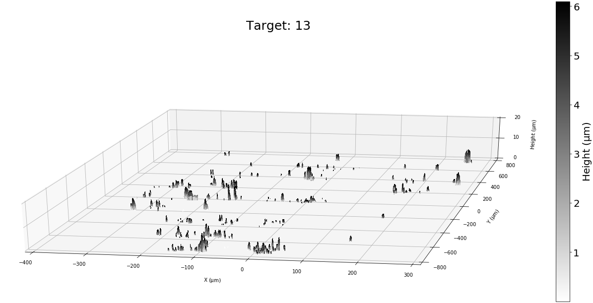
Fig 1. 3D dust coverage map of target 13
We find there is only a weak trend between shape descriptors and cometary source regions, cluster morphology, and particle characteristics such as size and particle morphology. For example, particles ejected from smooth or rough terrain are similar in their investigated shape properties, which implies dust particle activity such as dust ejection, partial dry out, and recycled dust material are not responsible for the structure of particles at the micrometre scale. Furthermore, the aspect ratio distributions suggest that the subunits of different cluster types are similar in their shape and composition. Thus, the different cluster morphologies detected by MIDAS are not created by a change in subunit properties, but rather by different impact velocities, a result in good agreement with the finding of laboratory experiments (Ellerbroek et al. 2017) and simulations (Lasue et al. 2019). Next, the types of clusters found in MIDAS show good agreement (Ellerbroek et al. 2017), however, there are some differences to those found by COSIMA (Lasue et al. 2019). Furthermore, our pristinity score shows that almost half of MIDAS particles suffered severe alteration by impact, which indicates dust alteration was inevitable with the given dust collection strategy. Consequently, only ~ 20 particles were rated 'moderately pristine' particles, i.e., they are not substantially flattened by impact, not fragmented, and/or not part of a fragmentation cluster. The microphysical properties of pristine cometary materials are established in this study and can be translated into properties of laboratory analogue materials for future study to understand comets and early Solar System processes.
How to cite: Kim, M., Mannel, T., Lasue, J., Longobardo, A., Bentely, M., and Moissl, R.: Primitiveness of cometary dust collected by MIDAS on-boardRosetta, Europlanet Science Congress 2022, Granada, Spain, 18–23 Sep 2022, EPSC2022-3, https://doi.org/10.5194/epsc2022-3, 2022.
Comets, thought to be amongst the most primordial of Solar System objects, are distinguished by their activity, i.e. the insolation driven ejection of gas and dust from their surfaces. The exact mechanisms of the outgassing and dust ejection remain an important open question in planetary science, relating as it does to the structure, composition, and thermophysical properties of the surface material. Various thermophysical models (see e.g. [1,2,3]) have been proposed to explain the activity seen by Rosetta at 67P/Churyumov-Gerasimenko, with these often compared to the total outgassing rate. Another directly observable effect of the activity, however, is the resultant non-gravitational force and torque on the cometary nucleus, which can alter its trajectory and rotation state. Understanding the effect of non-gravitational forces on the dynamics of a particular comet therefore gives us a powerful additional tool to investigate its activity and surface properties.
Here we present the latest work in an ongoing project, testing various activity distributions in an effort to fit the combined Rosetta outgassing, trajectory, and rotation data. We test a number of different activity distributions over the surface of the comet by varying the Effective Active Fraction (EAF) of facets on a shape model, relative to a pure water-ice emission. We investigate different spatial patterns in EAF, and attempt to correlate them to physical features on the cometary surface. In addition to the changes in rotation period examined in [4], we also compute changes in the rotation axis, using a method based on [5] in order to compare with the observations. This provides an additional constraint on the spatial distribution of activity. Trajectory information, in the form of Earth-to-comet range, is also compared with a recent re-analysis of Rosetta radio-tracking data [6].
We are able to achieve a reasonable fit to the combined Rosetta data by parameterising EAF in terms of the different geological unit types on 67P (Fig. 1). This will have important implications for understanding how activity works on the different types of surface observed on cometary nuclei, including ‘rough’, ‘smooth’, ‘dusty’ and ‘rocky’ surface morphologies. The objective here is to constrain the shape of the activity curve on these various surfaces that a more detailed thermal model must produce in order to fit the data. We are in the process of implementing these more advanced thermal models [1,3] in our code, and will present results of an analysis of the non-gravitational forces and torques generated by [1].
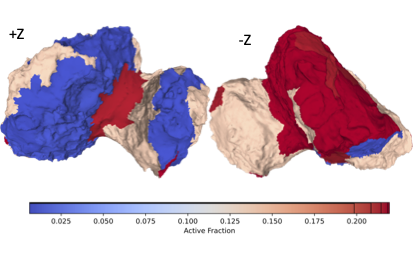
Fig. 1. Peak Effective Active Fraction over the surface of 67P for a model fit to geological unit types.
References
- How comets work. Fulle, M. Blum, J., Rotundi, A., 2019. ApJ Letters, 879:L8 (3pp).
- Near-perihelion activity of comet 67P/Churyumov–Gerasimenko. A first attempt of non-static analysis. Yu. Skorov, H. U. Keller, S. Mottola and P. Hartogh. Monthly Notices of the Royal Astronomical Society, Volume 494, Issue 3, May 2020, Pages 3310–3316
- On the activity of comets: understanding the gas and dust emission from comet 67/Churyumov-Gerasimenko’s south-pole region during perihelion. B. Gundlach, M. Fulle, J. Blum. Monthly Notices of the Royal Astronomical Society, Volume 493, Issue 3, April 2020, Pages 3690–3715
- Constraining models of activity on comet 67P/Churyumov-Gerasimenko with Rosetta trajectory, rotation, and water production measurements. N. Attree, L. Jorda, O. Groussin, S. Mottola, N. Thomas, Y. Brouet, E. Kührt. Astronomy & Astrophysics 630, A18
- Kramer, T., Laeuter, M., Hviid, S., et al. 2019. A&A, Volume 630, id.A3, 11 pp.
- Lasagni Manghi R., Zannoni M., Tortora P., Kueppers M., O'Rourke L., Martin P., Mottola S., et al., 2020, EGU General Assembly 2020, Online, 4–8 May 2020, EGU2020-19173
How to cite: Attree, N., Argawal, J., Jorda, L., Groussin, O., Marschall, R., Lasagni Manghi, R., Tortora, P., and Zannoni, M.: Constraints on comet thermal models from Rosetta at 67P/Churyumov-Gerasimenko, Europlanet Science Congress 2022, Granada, Spain, 18–23 Sep 2022, EPSC2022-5, https://doi.org/10.5194/epsc2022-5, 2022.
Introduction
The ESA Rosetta mission orbited the 67P/Churyumov-Gerasimenko comet (hereafter 67P) for two years and its results are providing important clues to understand activity processes on comets.
The goal of the ISSI International Team “Characterization of 67P cometary activity” is two-fold:
- Retrieval of the activity of different regions of 67P’s surface during different time periods.
- Identification of the main drivers and the effects of cometary activity, via revealing the link between cometary activity and illumination/local time, dust morphology and composition, and surface geomorphology.
Goal #1 has been reached by tracing the motion of dust particles detected in the coma back to the nucleus surface.
Goal #2 accomplishment is in progress by means of data fusion of different instruments onboard the Rosetta spacecraft.
Traceback
The Grain Impact Analyser and Dust Accumulator (GIADA) [1] measured speed and momentum of fluffy and compact dust particles. We assumed radial motion, constant dust acceleration up to a 11 km altitude and constant speed above that height, to retrieve the source region of each dust particle detected in the coma [2]. We obtained that fluffy and compact dust distributions correlate on the surface, but not in the coma due to the different speeds of the two dust categories. Dust ejection is also correlated with solar illumination. Fluffy particles are more abundant in rough terrains [3], according to models which predict that they are embedded within pebbles [4].
Traceback is under study also with a different approach, based on retrieving ejection probability maps of detected dust particles [5].
Data Fusion
GIADA vs VIRTIS. We related dust ejection rates of different surface regions, as retrieved by GIADA, and spectral indicators of water ice exposure measured by the Visible InfraRed Thermal Imaging Spectrometer (VIRTIS) of Rosetta, such as the shortward shift of the 3.2 mm absorption band center and infrared spectral slope flattening [2]. The observed correlation between these parameters (Figure 1) indicates that ejection of dust comes from water ice-rich regions.

Figure 1. Observed correlation between number of fluffy particles ejected from each 67P surface region and observed infrared slope flattening. Each symbol identifies a different geomorphological region of 67P.
GIADA vs MIDAS. The Micro-Imaging Dust Analysis System (MIDAS) detected and measured physical properties of micron-sized particles. In principle, it provides complementary information with respect to GIADA, which detected mm-sized particles.
We retrieved the number of parent particles hitting the MIDAS targets by applying two different methods [7,8]. Independently of the used approach, we obtained that the dust flux ratio between the two instruments is temporally constant. This suggests that the small particles detected by MIDAS are fragments of larger particles, as those detected by GIADA.
The combination of MIDAS data and our traceback algorithm revealed that the physical properties (size, density, flatness) of compact dust are homogeneous across 67P’s surface (Figure 2). Indicators of dust pristinity were defined [8] and suggested that pristinity is correlated with size (being small particles more pristine) but not with the ejecting region evolution degree.

Figure 2. Flatness distribution of dust particles detected on different MIDAS target (each target corresponds to a defined exposition period). Distributions are very similar.
GIADA vs ROSINA. ROSINA-COPS (Rosetta Orbiter Spectrometer for Ion and Neutral Analysis - COmetary Pressure Sensor) detected icy particles as pressure peaks [9]. The GIADA-ROSINA data fusion allows us to associate icy and dust particles and to retrieve the icy particle source regions.
Currently, a moderate correlation between icy and dust fluffy dust particles was found. The work is in progress.
Conclusions and future perspectives
. We found that fluffy dust particles are more abundant on rough terrains, in agreement with their lower evolution degree and to comet formation models. Physical properties of compact dust are similar across the comet surface. The relation between dust and icy particles is under study.
Future activities include:
- Analysis of the COSIMA mass spectrometer data [10], which observed dust composition variations. COSIMA-GIADA data fusion will allow understanding if they are related to different surface terrains.
- Analysis of OSIRIS images, which show bright patches on the comet surface, corresponding to frost enrichments and having different composition and morphology [11]. OSIRIS images combined with GIADA and ROSINA data will help in characterizing these peculiar regions.
- Laboratory activity aimed at simulating and interpreting the different photometric behavior of rough and smooth terrains [12] at the dust scale
References
[1] Della Corte, V. et al. (2014), Journal of Astronomical Instrumentation, 3, 1, 1350011-110; [2] Longobardo, A. et al. (2019), MNRAS, 483, 2, 2165-2176; [3] Longobardo, A. et al. (2020), MNRAS, 496, 1, 125-137; [4] Fulle, M. and Blum, J. (2017), MNRAS, 492, 2, S39-S44; [5] Ivanovski, S.L. et al. (2017), EPSC, 708; [6] Bentley, M.S. et al. (2016), Nature, 537, 7618, 73-75; [7] Longobardo, A. et al. (2020), EPSC, 1044; [8] Kim, M. et al. (2022), EGU abstract; [9] Pestoni, B. et al. (2022), EPSC, this session; [10] Hilchenback, M. et al. (2019), EPSC, 900; [11] Dehapriya, J.D.P. et al. (2018), EPSC, 1166; [12] Longobardo, A. et al. (2017), MNRAS, 469, 2, S346-S356.
Acknowledgements
This research was supported by the Italian Space Agency (ASI) within the ASI-INAF agreement I/032/05/0 and by the International Space Science Institute (ISSI) through the ISSI International Team “Characterization of cometary activity of 67P/Churyumov-Gerasimenko comet”.
M.K. and T.M. acknowledge funding by ESA project "Primitiveness of cometary dust collected by MIDAS on-board Rosetta" (Contract No. 4000129476).
How to cite: Longobardo, A., Kim, M., Pestoni, B., Cottin, H., Guttler, C., Ivanovski, S., Mannel, T., Merouane, S., Rinaldi, G., Rubin, M., Tubiana, C., Zakharov, V., Deshapriya, P., Dirri, F., Ciarniello, M., Della Corte, V., Fulle, M., Palomba, E., and Rotundi, A.: Characterization of 67P/Churyumov-Gerasimenko cometary activity, Europlanet Science Congress 2022, Granada, Spain, 18–23 Sep 2022, EPSC2022-459, https://doi.org/10.5194/epsc2022-459, 2022.
Centaurs are small objects of the Solar System with orbits between Jupiter and Neptune (5.2 AU < q < 30 AU) (Jewitt 2009), being an important population due to the presence of cometary activity (about 13% of Centaurs shows cometary activity) (Bauer et al. 2008). However, after the discovery of ring systems orbiting Chariklo (Braga-Ribas et al. 2013) and Haumea (Ortiz et al. 2017) and the proposition of a ring around Chiron (Ruprecht et al. 2015; Ortiz et al. 2015), we wonder if these structures are common around the small bodies or if specific conditions are necessary for their formation and maintenance (Sicardy et al. 2020). Discovered in March 2000, the active Centaur 174P/Echeclus (60558) has an equivalent diameter estimated in 59 ± 4 km (Bauer et al. 2013) and 64.6 ± 1.6 km (Duffard et al. 2014), and showed cometary activity on different occasions: December 2005 (Choi & Weissman 2006), May 2011 (Jaeger et al. 2011), August 2016 (Miles 2016), and December 2017 Kareta et al. (2019). To determine the main body’s size and shape and investigate whether material ejections during the outbursts could have fed possible rings or a shell of diffuse material around Echeclus, we predicted and observed stellar occultations by this Centaur in 2019, 2020, and 2021.
Stellar occultations by Echeclus were predicted using the Gaia DR2 catalog and NIMA ephemeris (Desmars et al. 2015). The prediction map of the 2019 October 29 event put the shadow’s path over South America, but all the telescopes that participated in this campaign missed the occultation path, providing five negative chords. The 2020 January 22 event is also predicted to pass over South America, resulting in two positive and four negative chords. Finally, we predicted the last event over Japan in 2021 January 19, resulting in one positive and ten negative chords.
With the positive detections of 2020, we fit an ellipse with an equivalent diameter of 59 ± 4 km to the edges of the chords. The resulting ellipse has a semi-major axis a’ = 36 km and oblateness ε′ = 0.325. From the rotational light curves (Rousselot et al., 2021), we note that 2020 stellar occultation occurs near the maximum absolute brightness. Thus, the surface seen during the occultation event was close to the maximum possible. So we were able to compare the ellipse fitted to the chords to the 3D model and pole orientations proposed by (Rousselot et al. 2021). By propagating the Echeclus rotation, we compare the 3D model to the 2021 stellar occultation, where we rule out some of the proposed pole solutions due to the close negative chord. We also fitted the 3D model to the chords, obtaining the triaxial dimensions of Echeclus as a × b × c = 36.5 × 28.0 × 24.5 km, resulting in an area-equivalent diameter of Dequiv = 61.8 ± 0.6 km, which is in agreement with the area-equivalent diameters presented in the literature.
We used all three event data sets to look for sudden drops in flux (evidence of confined material) or shallow and extensive drops (evidence of coma). The best light curves in terms of spatial resolution and SNR were: La Silla/NTT in 2019, which covered about 7,000 km in the sky plane; SOAR in 2020, covering 14,000 km in the sky plane and Okazaki/Japan in 2021, which covered about 9,000 km in the sky plane. With these light curves, we determined lower limits for detection for apparent opacity at the 3σ level as 0.145, 0.189, and 0.258, respectively. In addition, limits for the equivalent width were also determined for these three data sets, with values of 0.19 km for La Silla/NTT, 0.36 km for SOAR, and 0.18 km for Okazaki.
Acknowledgments: C.L.P. is thankful for the support of the CAPES scholarship. The following authors acknowledge the respective CNPq grants: F.B-R 309578/2017-5; J.I.B.C. 308150/2016-3 and 305917/2019-6; F.L.R. CAPES scholarship. This study was financed in part by the Coordenação de Aperfeiçoamento de Pessoal de Nível Superior - Brasil (CAPES) - Finance Code 001 and the National Institute of Science and Technology of the e-Universe project (INCT do e-Universo, CNPq grant 465376/2014-2). ARGJr acknowledges FAPESP grant 2018/11239-8.
References
Bauer, J. M., Choi, Y.-J., Weissman, P. R., et al. 2008, PASP, 120, 393
Bauer, J. M., Grav, T., Blauvelt, E., et al. 2013, The Astrophysical Journal, 773, 22
Braga-Ribas, F., Sicardy, B., Ortiz, J. L., et al. 2013, ApJ, 773, 26
Choi, Y.-J. & Weissman, P. 2006, in AAS/Division for Planetary Sciences Meeting Abstracts, Vol. 38, 37.05
Desmars, J., Camargo, J. I. B., Braga-Ribas, F., et al. 2015, A&A, 584, A96
Duffard, R., Pinilla-Alonso, N., Santos-Sanz, P., et al. 2014, A&A, 564, A92
Jaeger, M., Prosperi, E., Vollmann, W., et al. 2011, IAU Circ., 9213, 2
Jewitt, D. 2009, AJ, 137, 4296
Kareta, T., Sharkey, B., Noonan, J., et al. 2019, AJ, 158, 255
Miles, R. 2016, CBET, 4313
Ortiz, J. L., Duffard, R., Pinilla-Alonso, N., et al. 2015, A&A, 576, A18
Ortiz, J. L., Santos-Sanz, P., Sicardy, B., et al. 2017, Nature, 550, 219
Rousselot, P., Kryszczyńska, A., Bartczak, P., et al. 2021, MNRAS, 507, 3444
Ruprecht, J. D., Bosh, A. S., Person, M. J., et al. 2015, Icarus, 252, 271
Sicardy, B., Renner, S., Leiva, R., et al. 2020, The Trans-Neptunian Solar System, 249
How to cite: Pereira, C. L., Braga-Ribas, F., Emilio, M., Morgado, B. E., Desmars, J., Sicardy, B., Ortiz, J. L., Vieira-Martins, R., Branco, H. C., Assafin, M., Camargo, J. I. B., Gomes-Jr, A., and Rommel, F. L. and the Echeclus team: Recent results of stellar occultations by (60558) Echeclus, Europlanet Science Congress 2022, Granada, Spain, 18–23 Sep 2022, EPSC2022-557, https://doi.org/10.5194/epsc2022-557, 2022.
We report on the results of a long photometry and monitoring of comet C/2017 K2 (PanSTARRS), hereafter 17K2, with the TRAPPIST telescopes [1]. 17K2 is an Oort cloud comet discovered by the Pan-STARRS survey in 2017 [2], at a large heliocentric distance of 16 au. The comet was later identified in archival imagery to be active at 23.8 au from the Sun, the second most distant discovery of an active comet [3]. It has been claimed that 17K2 is a rare CO-rich comet [4]. We started observing 17K2 with TRAPPIST-North on October 25, 2017 using broad-band filters when the comet was at 15 au from the Sun with a magnitude of 18. We started collecting broad and narrow-band images [5] with TRAPPIST-South on September 9, 2021 (rh=5.4 au) when the comet became visible and bright from the southern hemisphere. The comet will reach its perihelion on December 19, 2022 at rh=1.8 au, and we will monitor its activity on both sides of perihelion. As writing this abstract, we detected emission of CN, C2, and C3 radicals as well as the dust continuum in four bands. By fitting the observed gas profiles with Haser model [6] after subtraction of the dust continuum, we derived the gas production rates for a different detected species. From the continuum and broad-bands images, we computed the Afρ parameter, and a dust production proxy [7]. In this work, we will show the magnitude evolution of this comet over 4 years (2017-2022), as well as the gas and dust activity for several months as a function of heliocentric distances.
References
[1] E. Jehin et al. 2011, The Messenger, 145, 2-6.
[2] Kaiser, N., Aussel, H., Burke, B. E., et al. 2002, Proc. SPIE, 4836, 154.
[3] Meech, K. J., Kleyna, J. T., Hainaut, O., et al. 2017, ApJL, 849, L8
[4] Yang, B., Jewitt, D., Zhao, Y., et al. 2021, ApJL, 914, L17
[5] Farnham, T. L., Schleicher, D. G., A’Hearn, M. F. 2000, Icarus, 147, 180
[6] L. Haser. 1957, Bulletin de l’Acad ́emie Royale de Belgique, Vol. 43, 740-750.
[7] Michael F. A’Hearn et al. 1984, The Astronomical Journal, Vol. 89, 579-591.
How to cite: Hmiddouch, S., Jehin, E., Moulane, Y., Jabiri, A., Vander Donckt, M., and Benkhaldoun, Z.: Monitoring the activity and composition of comet C/2017K2 (PanSTARRS) with TRAPPIST telescopes, Europlanet Science Congress 2022, Granada, Spain, 18–23 Sep 2022, EPSC2022-593, https://doi.org/10.5194/epsc2022-593, 2022.
Eris is currently the most massive known dwarf planet in the Solar system, it has one known satellite, Dysnomia (Brown & Schaller 2007; Holler et al. 2020). There have been several attempts trying to identify the rotation period of Eris from visible ground based measurements which resulted in a wide range of possible values (Duffard et al., 2008). Here we present some new light curve data of Eris, taken with ∼1m-class ground based telescopes, with the GROND instrument at the 2.2m MPG/ESO telescope La Silla, and also with the Transiting Exoplanet Survey Satellite (TESS).
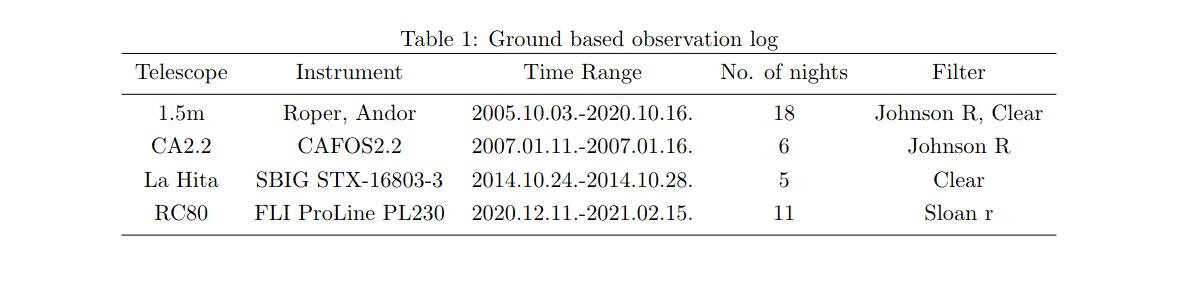
Observations of Eris with GROND were made in 3 nights in August 2010. Auxiliary ground based photometry data of Eris from five telescopes were obtained in irregular intervals between 2005 and 2020 (see table 1.) TESS observed Eris in Sector 30 with its Camera 1 and CCD 3. A significant portion of the light curve data had to be excluded due to Eris’ encounter with nearby background sources which left a dominant feature in the background-subtracted image. We note that due to the limited length of the TESS light blocks (2.3 d and 6.6 d) it was not possible to detect light curve periods in to order or close to the orbital period (15.78 d).
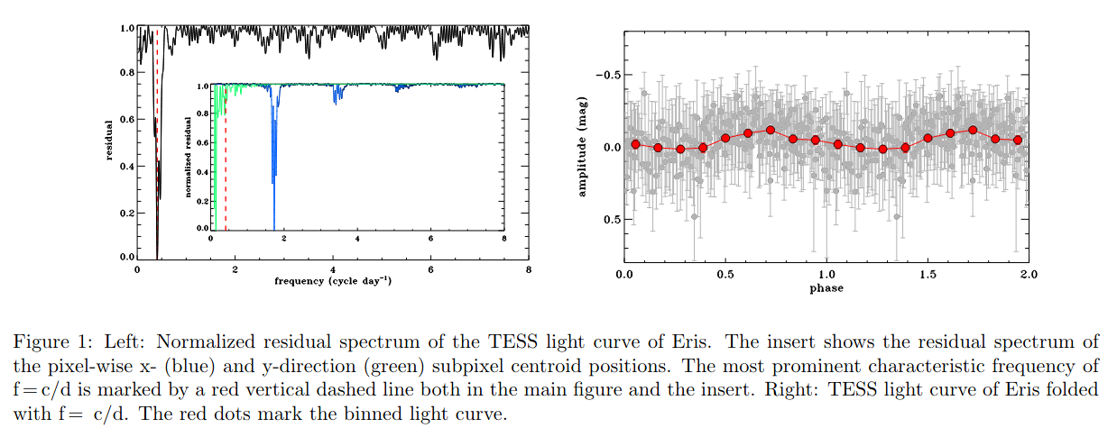
For most of the ground-based measurements we used our night-averaged values for the 1.5m, La Hita and CA2.2m data), except for the GROND measurements, for which we used the all the individual data points. In addition, we also considered previously published data, including ground-based data from Carraro et al., 2006 and Duffard et al., 2008, and the SWIFT satellite data from Roe et al., 2008.
We assumed that i) the light curve amplitude is the same in any of the photometric bands used and ii) the light curve can be described by a simple sinusoidal variation. With these assumptions each model light curve can be described by four parameters: a light curve amplitude, period, phase-shift, and an offset from the photometric zero point. We allowed a different offset for each measurement block even if the data were taken by the same instrument and filter combination (1.5m measurements) due to the year-long gaps between the measurement blocks. We chose an amplitude A and period P, and determined the best fitting light curve phase using a Levenberg–Marquardt minimization algorithm. We expect that the best-fitting period-amplitude values provide the lowest C(P,A) values. We searched the period range P ∈ [1d, 15.88 d], where 15.88 d is the orbital period of Dysnomia, and it would correspond to a synchronised rotation. The C(P,A) contour map shows two minima, one at P ≈ 8 h, and A ≈ 0.05, and another at P ≈ 11.5 h, and A ≈ 0.08. To check the robustness of this result, we repeated the process by modifying the photometric data points by adding a random value with normal distribution and repeating the fitting process several times for the whole data set. The same two minima popped up in all cases. TESS data favours a rotation period of 59.420±0.527 h (See Figure 1.), while ground based data is more compatible with a synchronous or nearly synchronous rotation (See Figure 2.).
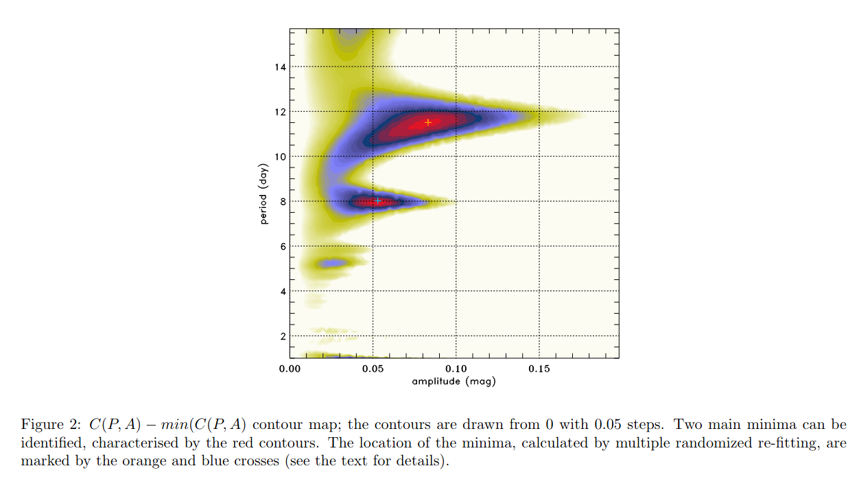
We inspected the colours calculated from the GROND photometry and compared our results to previous values from the literature (Table 2). The optical colours (B-V, V-R, R-I) are in good agreement with previous colours, but the J-H colour from GROND is different from the ones in the literature. Also, we can see a big scatter in those. (See Table 2.)
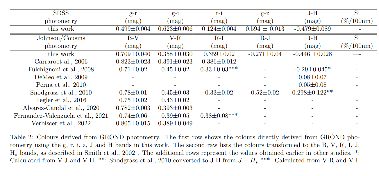
One possible explanation can be, that there is a big CH4 feature on the surface of Eris, which has strong absorption lines in H band, and it can change the NIR colour, but not the optical ones. To confirm this, more long-term optical and NIR measurements are needed. Finally, we use the simple tidal evolution code by Hastings et al. (2016) to calculate the evolution of the satellite orbit (only the semi-major axis in this approximation) and the spin evolution of Eris and Dysnomia. Although the spin period of Eris is not well defined yet, it is an interesting question whether the possible rotation periods of Eris – ranging from a few hours to the orbit-synchronous state – are feasible in terms of tidal evolution, using the current knowledge on the system components.
How to cite: Szakáts, R., Kiss, C., Pál, A., Müller, T., Greiner, J., Santos-Sanz, P., Marton, G., Ortiz, J. L., Morales, N., Duffard, R., and Sági, P.: On the rotation of the dwarf planet (136199) Eris, Europlanet Science Congress 2022, Granada, Spain, 18–23 Sep 2022, EPSC2022-824, https://doi.org/10.5194/epsc2022-824, 2022.
The phase curve of a small Solar System object shows the change in the object’s reflectance at different Sun-object-observer (phase) angles, and the shape of the phase curve is determined by the physical properties of the object’s surface. Analysing phase curves of small Solar System objects such as Kuiper belt objects (KBOs), Centaurs, and inert Jupiter-family comets (JFCs) can also probe the composition and regolith structure of their surfaces, and by comparing these across populations of objects, can reveal possible evolutionary connections between them.
The phase curve of an object can be significantly altered from its nominal shape if the object has undergone epochs of cometary activity during the time across which observations were taken. Furthermore, Centaur activity takes the form of outgassing in between long periods of quiescence, differing significantly from the activity exhibited by JFCs, which is more continuous and strongly coupled to heliocentric distance. As a result, Centaur activity may be difficult to identify from their phase curves if there are large time-intervals between observations. However, if observations are taken at sufficiently high cadence to isolate these outbursts, phase curves can be used to detect and analyse cometary activity out to distances where any coma may not be visible to Earth-based observations. This technique can help shed light on the mechanism responsible for the activity exhibited by Centaurs, which is presently not fully understood, and which is also an important step in understanding cometary evolution in the Solar System.
Obtaining such high cadence observations over multiple apparitions for phase curve analysis is difficult to achieve due to limited availability of telescope observation time, the large baseline of observations required, and the challenges of ground-based observing (poor weather and the limited observability of targets throughout the year). To circumvent these difficulties, many previous studies of phase curves augment their datasets by collating photometry obtained from different sources (Alvarez-Candal et al., 2016; Ayala-Loera et al., 2018; Alvarez-Candal et al., 2019). These additional data are often obtained with heterogeneous methods of image processing and data analysis, which might introduce systematic errors in the resulting phase curve. The Asteroid Terrestrial-impact Last Alert System (ATLAS) survey (Tonry et al., 2018a,b) has accumulated serendipitous observations of several bright KBOs, Centaurs, and JFCs, having observed the visible sky over a 2-day cadence, to a limiting magnitude of ~19.5 in two wide-band filters since it first began observations in 2015. ATLAS offers an opportunity to study the phase curves of these objects populated with large datasets and thus use them to search for epochs of cometary activity.
Using data from the Haleakalā and Mauna Loa telescopes of the ATLAS 4-telescope survey, we analyse the phase curves of the bright KBOs, Centaurs, and JFCs visible to ATLAS with datasets large enough that we do not need to include additional data from potentially heterogeneous sources, thereby reducing potential systematic errors. Our sample of 18 bright KBOs, JFCs and Centaurs visible to ATLAS span semimajor axes of 5.7 au ≤ a ≤ 67.9 au, absolute magnitudes of −1.1 < HV < 13.3. Each object has on average 181 (c-filter) and 463 (o-filter) data points, exceeding the values of previous studies (Rabinowitz et al., 2007; Schaefer et al., 2009; Alvarez-Candal et al., 2016; Ayala-Loera et al., 2018; Alvarez-Candal et al., 2019), and which sample most of the phase angle range observable from Earth.
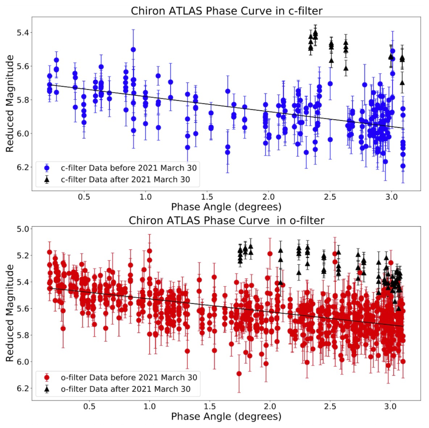
Figure 1: From Dobson et al. (2021), ATLAS Phase Curves of (2060) Chiron in c-filter (upper plot) and o-filter (lower plot), with data from most recent apparition indicated as black triangles. Black lines represent linear best fits to data.
We present our findings on using ATLAS phase curves with their advantage of unprecedentedly large datasets to search for instances of cometary activity exhibited by our sample of KBOs, JFCs and Centaurs since 2015. Notably, we discover a recent brightening of the Centaur (2060) Chiron (Dobson et al. 2021), as seen in Figure 1, which despite the lack of detected coma, is indicative of either an outburst or enhanced activity.
Acknowledgements
We made use of the ATLAS Forced Photometry Server to obtain our Centaur and KBO photometry. https://fallingstar-data.com/forcedphot/
This work has made use of data from the Asteroid Terrestrial-impact Last Alert System (AT- LAS) project. ATLAS is primarily funded to search for near earth asteroids through NASA grants NN12AR55G, 80NSSC18K0284, and 80NSSC18K1575; byproducts of the NEO search include images and catalogs from the survey area. The ATLAS science products have been made possible through the contributions of the University of Hawaii Institute for Astronomy, the Queen’s University Belfast, the Space Telescope Science Institute, the South African Astronomical Observatory (SAAO), and the Millennium Institute of Astrophysics (MAS), Chile.
References
Alvarez-Candal, A., Ayala-Loera, C., Gil-Hutton, R., et al. 2019, MNRAS, 488, 3035, doi: http://doi.org/10.1093/mnras/stz188010.1093/mnras/stz1880
Alvarez-Candal, A., Pinilla-Alonso, N., Ortiz, J. L., et al. 2016, A&A, 586, A155, doi: http://doi.org/10.1051/0004-6361/20152716110.1051/0004-6361/201527161
Ayala-Loera, C., Alvarez-Candal, A., Ortiz, J. L., et al. 2018, MNRAS, 481, 1848, doi: http://doi.org/10.1093/mnras/sty236310.1093/mnras/sty2363
Dobson, M. M., Schwamb, M. E., Fitzsimmons, A., et al. 2021,
Research Notes of the AAS, 5, 9, doi: http://doi.org/10.3847/2515-5172/ac26c9
Rabinowitz, D. L., Schaefer, B. E., & Tourtellotte, S. W. 2007, AJ, 133, 26, doi: http://doi.org/10.1086/50893110.1086/508931
Schaefer, B. E., Rabinowitz, D. L., & Tourtellotte, S. W. 2009, AJ, 137, 129, doi: http://doi.org/10.1088/0004-6256/137/1/12910.1088/0004-6256/137/1/129
Tonry, J. L., Denneau, L., Heinze, A. N., et al. 2018a, , 130, 064505, doi: http://doi.org/10.1088/1538-3873/aabadf10.1088/1538-3873/aabadf
Tonry, J. L., Denneau, L., Flewelling, H., et al. 2018b, ApJ, 867, 105, doi: http://doi.org/10.3847/1538-4357/aae38610.3847/1538-4357/aae386
How to cite: Dobson, M. M., Schwamb, M. E., Benecchi, S. D., Verbiscer, A. J., Fitzsimmons, A., Shingles, L. J., Denneau, L., Heinze, A. N., Smith, K. W., Tonry, J. L., Weiland, H., and Young, D. R.: Using Phase Curves from ATLAS to Search for Cometary Activity in the Solar System, Europlanet Science Congress 2022, Granada, Spain, 18–23 Sep 2022, EPSC2022-878, https://doi.org/10.5194/epsc2022-878, 2022.
The Rosetta mission of the European Space Agency has enabled a deep study of the nucleus and coma of comet 67P/Churyumov-Gerasimenko (hereafter 67P). Four instruments onboard the Rosetta spacecraft sensed coma particles ejected from the nucleus of 67P: the Grain Impact Analyzer and Dust Accumulator (GIADA; Della Corte et al. 2014), the COmetary Secondary Ion Mass Analyser (COSIMA; Kissel et al. 2007), the Micro-Imaging Dust Analysis System (MIDAS; Riedler et al. 2007), and the COmet Pressure Sensor (COPS; Balsiger et al. 2007). GIADA, COSIMA, and MIDAS were developed specifically for the study of cometary dust. COSIMA and MIDAS are sensitive only to refractories, GIADA is sensitive to refractories and (semi-)volatiles. On the other hand COPS is a gas density and pressure sensor that unexpectedly perceived the sublimating volatile fraction of cometary particles (Pestoni et al. 2021a,b). Since COPS measured a different component than the other three instruments, a comparison of the results of the latter is particularly worthy. In this study, we investigate correlations among the particle detections of COPS and GIADA.
The two COPS gauges – the nude gauge (hereafter NG) and the ram gauge (hereafter RG) – detected 6.7e4 and 73 dust particles, respectively. GIADA subsystems led to the identification of 2110 compact particles, 3159 fluffy fragments arose by the fragmentation of 277 parent particles, and 4e-7 kilograms of mass coming from nanogram dust particles (Della Corte et al. 2019). It has been found that NG detections are correlated solely with GIADA parent particles, meaning that fluffy particles have both a volatile and a refractory part. Parent particles are fragmented by the spacecraft potential (Fulle et al. 2015). Consequently, the NG may not have observed intact parent particles, but one or more fluffy fragments reaching COPS remained unresolved within time resolution of the instrument. The diameters of equivalent water ice spheres calculated from the values of the density increases measured by the RG and the NG (60-850 nm assuming a density of 1 g cm−3; Pestoni et al. 2021a,b) are comparable to the sizes of the subunits of the fractal particles detected by MIDAS (52-183 nm; Mannel et al. 2019).
References
Balsiger, H., Altwegg, K., Bochsler, P. et al. 2007, Space Sci. Rev., 128, 745
Della Corte, V. et al. 2014, JAI, 3, 1, 1350011-110
Della Corte, V., Rotundi, A., Zakharov, V., et al. 2019, A&A, 630, A25
Fulle, M., Della Corte, V., Rotundi, A., et al. 2015, ApJ, 802, L12
Kissel, J., Altwegg, K., Clark, B. C., et al. 2007, Space Sci. Rev., 128, 823
Mannel, T., Bentley, M. S., Boakes, P. D., et al. 2019, A&A, 630, A26
Riedler, W., Torkar, K., Jeszenszky, H., et al. 2007, Space Sci. Rev., 128, 869
Pestoni, B., Altwegg, K., Balsiger, H., et al. 2021a, A&A, 645, A38
Pestoni, B., Altwegg, K., Balsiger, H., et al. 2021b, A&A, 651, A26
How to cite: Pestoni, B., Altwegg, K., Della Corte, V., Longobardo, A., Müller, D., Rotundi, A., Rubin, M., and Wampfler, S.: A multi-instrument analysis of 67P/Churyumov-Gerasimenko coma particles: COPS vs. GIADA, Europlanet Science Congress 2022, Granada, Spain, 18–23 Sep 2022, EPSC2022-971, https://doi.org/10.5194/epsc2022-971, 2022.
The long-period comet C/2017 K2 (PanSTARRS) was discovered in 2017 at a large heliocentric distance of 16 au (Wainscoat et al. 2017). Pre-discovery images from 2013 show that K2 was even active at a record distance of ~24 au from the Sun (Jewitt et al. 2017) well beyond the snow line, indicating that, most probably, CO and CO2 ices - the most abundant species after water - might drive its activity. CO was indeed detected in K2’s coma in the sub-mm range at a heliocentric distance of 6.7 au (Yang et al. 2021) and K2 was claimed to be a CO-rich comet.
Detecting comets at such large distances is becoming more frequent, but it is still a rare occasion to study a well preserved comet surface coming directly from the Oort Cloud or on a several million years orbit, and especially if it is of a rare type.
K2 will reach its perihelion on 2022 December 19 (Rh=1.8 au, Δ=2.5 au) and become a bright target in automn with good observing conditions from the Southern hemisphere. We have started an observing campaign on May 8 (Rh=3.2 au), 2022 with UVES at the ESO VLT to obtain high resolution and good SNR optical spectra to characterize the detailed coma composition of its daughter species before and after K2 perihelion. We report here about the first epochs before perihelion.
UVES was setup with a slit width of 0.45" (length of 10") to provide a resolving power of 80.000, and we selected two different settings (DIC#1 346/580 and DIC2 437/860) to cover the whole optical range (304-1040 nm) at each epoch in only two long exposures on the same night. These spectra will allow us to compare K2 - characterized by its unusual distant activity - to other well studied comets in the optical and particularly using the same instrument since 20 years by the Liège comet team. These spectra will allow us to measure the detailed composition of its coma: the production rates of the daughter species (OH, CN, C2 etc.) to check among other things if the comet is a C-chain depleted or normal comet (A'Hearn et al. 1995), to link those production rates with those from the parent species observed in the IR (see CRIRES+ poster by Lippi et al.), to search for CO+ and CO2+ lines to check if K2 is a CO-rich comet like the unique CO-N2-rich blue comet C/2016 R2 (PanSTARRS) (Opitom et al. 2019), to measure the ratio of the [OI] lines to estimate the CO/H2O ratio (Decock et al. 2015), and if the comet is bright enough to measure the isotopic ratios of the light elements (12C/13C and 14N/15N from the CN isotopologues), to measure the ortho- to para- ratio of NH2, and search for faint FeI and NiI lines which are a new and puzzling component of the cometary coma (Manfroid et al. 2021).
How to cite: Jehin, E., Lippi, M., Hutsemékers, D., Manfroid, J., Vander Donckt, M., and Rousselot, P.: Pre-perihelion high resolution optical spectroscopy of the long period comet C/2017 K2 (PanSTARRS) with UVES at the VLT, Europlanet Science Congress 2022, Granada, Spain, 18–23 Sep 2022, EPSC2022-1071, https://doi.org/10.5194/epsc2022-1071, 2022.
The discovery of trans-Neptunian objects (TNOs) marked an important milestone in the understanding of the outer Solar System. Due to their environmental conditions, these objects could preserve the most pristine materials that were present on the protoplanetary disk. Studies focused on understanding TNOs physical and dynamical properties can be used to probe planetary formation processes and the subsequent solar system dynamical evolution that followed the formation era.
Nowadays, above 3,000 TNOs have been detected, including four large ones that receive the official designation of dwarf-planets. Analysis of TNOs revealed a compositionally and dynamically diverse population. However, despite all the progress in the last decades, much is still unknown about the composition of the TNOs.
The recently launched James Webb Space Telescope (launched on December 25, 2021) will provide a powerful tool to investigate the TNOs surface composition, where all prior instrumentation has fallen short. The NIRSpec instrument onboard JWST will provide high-quality data that will surpass the quality of the data available by orders of magnitude. DiSCo-TNOs, lead by the Florida Space Institute, is the only large program approved by JWST for the study of the Solar System. With it, we aim to assess the relative ratio of water ice, complex organics, silicates, and volatiles on the surface of a large sample of TNOs. This information is vital to improving models of the formation of our Solar System and other planetary systems. In this talk we present the scope of the DiSCo program, and the tools that are being developed to extract the maximal information from the data. We pay special attention to the compositional modeling technique that uses an implementation of a nested sampling algorithm for Bayesian inference of the abundances and grain sizes distribution of the materials present on TNOs surfaces.
How to cite: De Pra, M., Pinilla-Alonso, N., Souza Feliciano, A. C., Schambeau, C., Harvison, B., Emery, J., Cruikshank, D., Pendleton, Y., Holler, B., Stansberry, J., Lorenzi, V., Muller, T., Guilbert-Lepoutre, A., Peixinho, N., Bannister, M., and Brunetto, R.: Discovering the Surface Composition of TNOs (DiSCo-TNOs) with the James Webb Space Telescope, Europlanet Science Congress 2022, Granada, Spain, 18–23 Sep 2022, EPSC2022-1196, https://doi.org/10.5194/epsc2022-1196, 2022.
SB4 | Computational astrophysics and numerical models of small bodies and planets
Recent sample-return missions to asteroids (101955) Bennu and (162173) Ryugu have revealed their rough surfaces are strewn with regolith particles ranging from millimeters to tens of meters in diameter with a broad spectrum of shapes. Numerical modelers often simulate these kinds of bodies as rubble piles composed of discrete particles with rock-like material properties. The particles in most models for the past few decades have been independent spheres meant to represent the individual grains that make up the surface and interior of a rubble pile. It has been shown, however, that grain shape has a significant effect on the flow and equilibrium states of particles in granular media. Simulating irregular grain shape is thus imperative for accurately modeling the surfaces and interiors of rubble-pile asteroids.
One of the most challenging aspects of simulations using spherical particles is creating high-porosity media. The densest packing distribution of monodisperse spheres has ~26% porosity; porosities of polydisperse spheres in a randomly packed orientation approach 35-45%. Bennu and Ryugu were each found to have bulk densities on the order of 1.1 g/cc, indicating bulk macroporosities of 50% or larger. Furthermore, the depth to which the arm of the OSIRIS-REx TAGSAM spacecraft penetrated Nightingale crater showed that it met little resistance from the regolith surface of Bennu, which may indicate that the finer-grained parts of regolith surfaces could have porosities larger than the bulk macroporosity. The low bulk densities and high macroporosities of rubble piles that have been visited by spacecraft seem to indicate subsurface structure mainly supported by contact networks between regolith grains strengthened by grain shape and interparticle cohesion from electrostatic and van der Waals forces. These recent results, in combination with historical measurements on the lunar surface, show a need to be more methodical in preparing “fluffy” granular beds to accurately reproduce surface structure on low-gravity, airless bodies.
For our experiments, we use the parallel N-body gravity tree code PKDGRAV. PKDGRAV uses a soft-sphere discrete element method to model surface grains as individual spheres that feel interparticle and uniform gravity, cohesion, and contact forces. The contact forces from the soft-sphere method allow particles to slightly interpenetrate at the point of contact, using a restoring spring force to model the stiffness (akin to the Young’s modulus) of the material and applying normal and tangential damping and forces like interparticle friction. More recently, we have made improvements to routines handling irregularly shaped “aggregate” particles, made by “gluing” together two or more spheres.
Aggregates allow PKDGRAV users to capture geometric effects like bulking, where low-sphericity polyhedra generally occupy larger volumes than spheres when packing, accounting for increased porosity and resistance to flow in granular media. With this in mind, we model the gentle deposition of aggregates under microgravity and lunar gravity to create highly porous (>50% porosity) granular assemblies both with and without cohesion. We use aggregates composed of centimeter-scale spheres and model both symmetric and asymmetric shapes, as well as systems with both aggregates and single spheres. We calculate the porosity of these systems by generating a concave hull around the settled system and calculating the ratio of the total volume in particles interior to the hull to the total hull volume, with interior particle volume modified to account for particle-particle overlaps and particle fractions partially exterior to the hull.
How to cite: DeMartini, J. and Richardson, D.: Modeling High-Porosity Regolith on Low-Gravity Planetary Surfaces, Europlanet Science Congress 2022, Granada, Spain, 18–23 Sep 2022, EPSC2022-560, https://doi.org/10.5194/epsc2022-560, 2022.
Many objects that form via a gravitational collapse or contraction appear to rotate around their own axis (spin) in a manner that aligns with their orbit around larger parent structures. Systematic prograde rotation is found in the planets and larger asteroids of the Solar System [1], in the stars of several open clusters [2], as well as in the molecular clouds of different galaxies [3,4]. Remarkably, the fact that such a spin-orbit alignment exists across different scales has received little scientific attention in the last decades, while a satisfactory answer remains to be found.
Indeed, when the rotational direction of an object is assumed to be equal to that of the cloud from which it formed, only specific birth environments with rising orbital velocity curves lead to systematic prograde spin [5]. We present a new mechanism that describes how collections of particles or clouds gain a prograde rotational component when they collapse or contract while subject to an external, central force. We show that because particles that orbit in any non-rigid cloud shear away from one another over time – and do so on curved paths – their combined center-of-mass moves inward. The orbital angular momentum that is thus liberated, adds a prograde component to the spin of the object that forms.
We first visualize the mechanism of prograde spin-up in Fig. 1a, where we plot the motion of a disk of particles on circular orbits around a central mass. For illustrative purposes, mutual interactions like self-gravity are not included here. Over time, the shear over curved orbits morphs the particles into an increasingly extended arc, whose combined center-of-mass moves inward to an orbit with a reduced semi-major axis. Hence, if the cloud of particles were to gravitationally collapse, the object forms at an orbit interior to the cloud, with a lower orbital angular momentum. The deficit goes into rotation, and the object attains a prograde spin. Being a geometric effect, the mechanism of prograde spin-up persists around any central potential that triggers shear, even those where the shear is strongly retrograde.
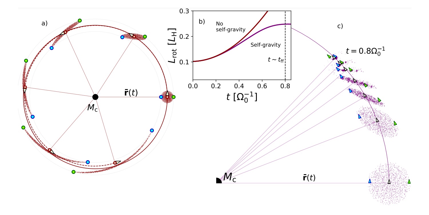
Fig. 1: Visual representation of the prograde spin-up mechanism
To verify this mechanism of prograde spin-up, we perform N-body simulations of gravitationally bound, collapsing clouds with REBOUND [6]. As seen in Fig. 1b, the rotational angular momentum of the cloud increases quadratically during the collapse (δLrot/LH ∝ t2), before slowing down when the collapse completes around t ∼0.8 tff in this example. We provide further visualization in Fig. 1c, where shear is seen to initially deform the cloud into a curved, bar-like structure whose center moves inward, spinning up the material. As the cloud contracts, collisions prevent further relative motion and eventually a stable, prograde binary forms.
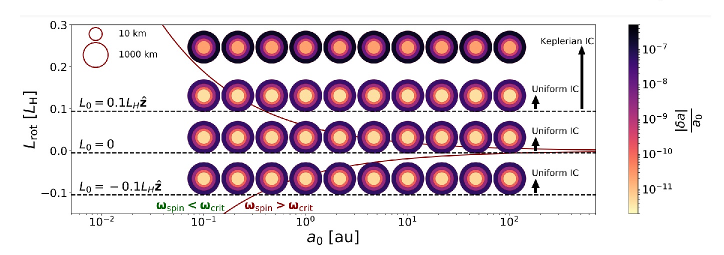
Fig 2: Rotational gain by prograde spin-up in the streaming instability.
We highlight an application of prograde spin-up to the rotation of (binary) asteroids in the Solar System, which are understood to form via gravitational collapse in a process known as the streaming instability [7]. We numerically estimate the magnitude of their spin-up with a set of N-body simulations with varying initial conditions (see Fig. 2). The formation of binaries is easier in the outer Solar System, offering an explanation for the high fraction of binary systems on wider orbits. Indeed, we show that at the distance of the Kuiper belt (∼30 AU), even the clouds that begin their collapse without any rotation can gain enough angular momentum via prograde spin-up to form prograde comet binaries.
Within the Solar System, the group of 'Cold Classicals' that reside in the Kuiper belt provide a unique sample of asteroids that likely retained their rotation at birth [8]. Besides being characterized by low inclinations and eccentricities, this group contains a high fraction of binary pairs [9] that often have strong color correlations [10], reinforcing the idea that they formed in a single gravitational collapse – rather than by later capture. The majority of these binaries spin in a prograde direction, a key signature that has recently been reproduced with detailed hydrodynamical simulations [8,11]. In these simulations, the colatitude distribution of the vorticity vectors is initially broad, and the prograde bias only appears when the bound clumps collapse. We suggest that the new mechanism of prograde spin-up can function as the physical driver of this rotational bias.
The relevance of prograde spin-up to the formation of objects by gravitational collapse on larger astrophysical scales remains open for further investigation. It is likely, however, that the universal applicability of prograde spin-up contributes to the ubiquity of spin-orbit alignment on different scales. The total rotational gain scales with relative cloud size: δLrot/LH ∝(Rcl/RH)5. Compared to the rotation contained in shear: δLrot/LH ∝(Rcl/RH)2, prograde spin-up becomes important when the size of the cloud prior to collapse is comparable to the Hill radius. For objects that form in this interface between self-gravity and shear, prograde spin-up naturally produces a spin-orbit alignment, even in an environment of retrograde shear.
[1] Grundy, W. M., Noll, K. S., Roe, H. G., et al. 2019, Icarus, 334, 62
[2] Corsaro, E., Lee, Y.-N., García, R. A., et al. 2017, Nature Astronomy, 1, 0064
[3] Braine, J., Rosolowsky, E., Gratier, P., Corbelli, E., & Schuster, K. F. 2018, A&A, 612, A51
[4] Braine, J., Hughes, A., Rosolowsky, E., et al. 2020, A&A, 633, A17
[5] Mestel, L. 1966, MNRAS, 131, 307
[6] Rein, H. & Liu, S. F. 2012, A&A, 537, A128
[7] Johansen, A., Youdin, A., & Mac Low, M.-M. 2009, ApJ, 704, L75
[8] Nesvorný, D., Li, R., Simon, J. B., et al. 2021, Planetary Science Journal, 2, 27
[9] Grundy, W. M., Noll, K. S., Roe, H. G., et al. 2019, Icarus, 334, 62
[10] Benecchi, S. D., Noll, K. S., Grundy, W. M., et al. 2009, Icarus, 200, 292
[11] Nesvorný, D., Li, R., Youdin, A. N., Simon, J. B., & Grundy, W. M. 2019, Nature Astronomy, 3, 808
How to cite: Brouwers, M. and Visser, R.: Prograde spin-up during gravitational collapse, Europlanet Science Congress 2022, Granada, Spain, 18–23 Sep 2022, EPSC2022-582, https://doi.org/10.5194/epsc2022-582, 2022.
SB5 | Tools for characterizing planetary and small bodies surfaces, atmospheres, and dust particles (Imagery, photometry, spectroscopy, spectrophotopolarimetry)
Abstract
The comet 17P/Holmes underwent an enormous outburst in October 2007 leaving vast amount of dust particles, which spread into elliptic orbits around the Sun [1, 2]. During February-March 2022 dust trail observations were forecasted to be possible with amateur sized telescope when outburst dust particles were in second revolution orbiting the Sun [1]. Observations were compared to the new dust trail particle model ‘Dust Trail kit’ implemented in Orekit.
1. Introduction
Cometary Dust Trail kit model was developed between 1999-2013 and latest dust trail observations were referenced to model at 2015 [1]. More recent observations were needed to ensure and validate model accuracy and these new observations were part of the announced comet 17P dust trail observation campaign that started in 2013 [1].
2. Observations
2.1 February 26th and 28th 2022
The 17P/Holmes dust trail was observed 26.2.2022 18:26UT and 28.8.2022 18:31UT based to the modeled position reported in [1]. 40 x 90 second exposures were taken at both nights with 305mm aperture telescope and clear filter using CCD bin2 mode and tracking stars. Stacked images were astrometrically plate solved and then subtracted and inverted to highlight the dust trails. Figure 1 shows the dust trails with their positions. The upper dark dust trail was observed on 26.2.2022 and lower light dust trail on 28.2.2022.
2.2 March 1st and 2nd 2022
The 17P/Holmes dust trail was observed on 1.3.2022 18:25UT and 2.3.2022 18:35UT based to the model position. CCD bin3 mode was used to get more sensitivity with exposure times 50 x 45 second at both nights. Images were then stacked, plate solved and subtracted. Figure 2 shows dust trails with positions, the upper dark dust trail is an observation made on 1.3.2022 and the lower light dust trail on 2.3.2022.
3. Comparison to the model
Observations 2.1 and 2.2 were compared with the results of the ‘Dust Trail kit’ model implemented in Orekit by Markku Nissinen. Figure 3 show a good correlation between the model calculations and the four observations.
4. Equipment and software
4.1 Equipment
The telescope used was 305mm aperture and 1205mm focal length F4 Newton with coma corrector. Mount was iOptron CEM60 and autoguider was configured to track stars during each exposure. The telescope was placed in Viestikallio Remote Controlled Observatory at Artjärvi, Finland under Bortle 3 rural sky conditions.
CCD-camera was cooled QSI690wsg having Sony ICX814 CCD-sensor. Exposures 90s and 45s were used with CCD binning 2x2 and 3x3, giving 1.3 and 1.9 arcsec/px resolution. Baader Clear filter was used.
4.2 Software
Image processing software used was PixInsight (PI), images were registered and stacked with PI Star registration and PI Integration functionality. PI PixelMath was used in image subtraction.
ASTAP software was used for plate solving and astrometric analysis.
5. Figures
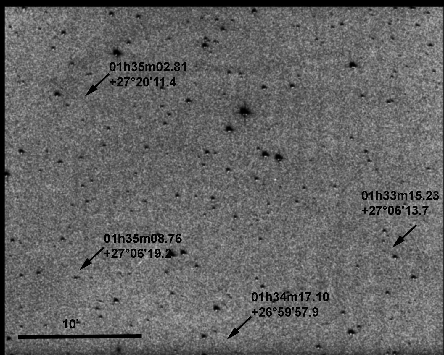
Figure 1: Subtracted image of 17P/Holmes dust trails with measured positions, upper dust trail 28.2.2022, lower trail 26.2.2022, Jorma Ryske. Observations separation is 48 hours.
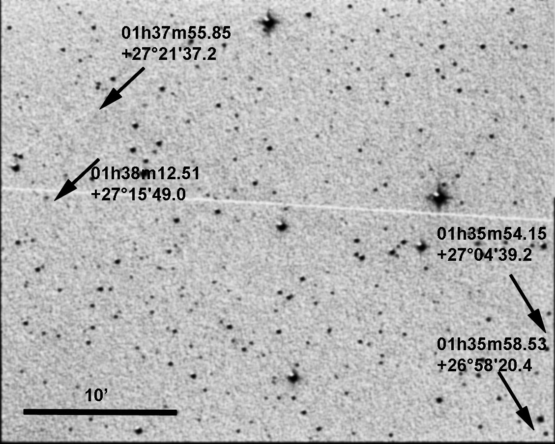
Figure 2: Subtracted image of 17P/Holmes dust trails with measured positions, upper dark dust trail 1.3.2022, lower light dust trail 2.3.2022, Jorma Ryske. Observations separation is 24 hours. Two satellite tracks in image.
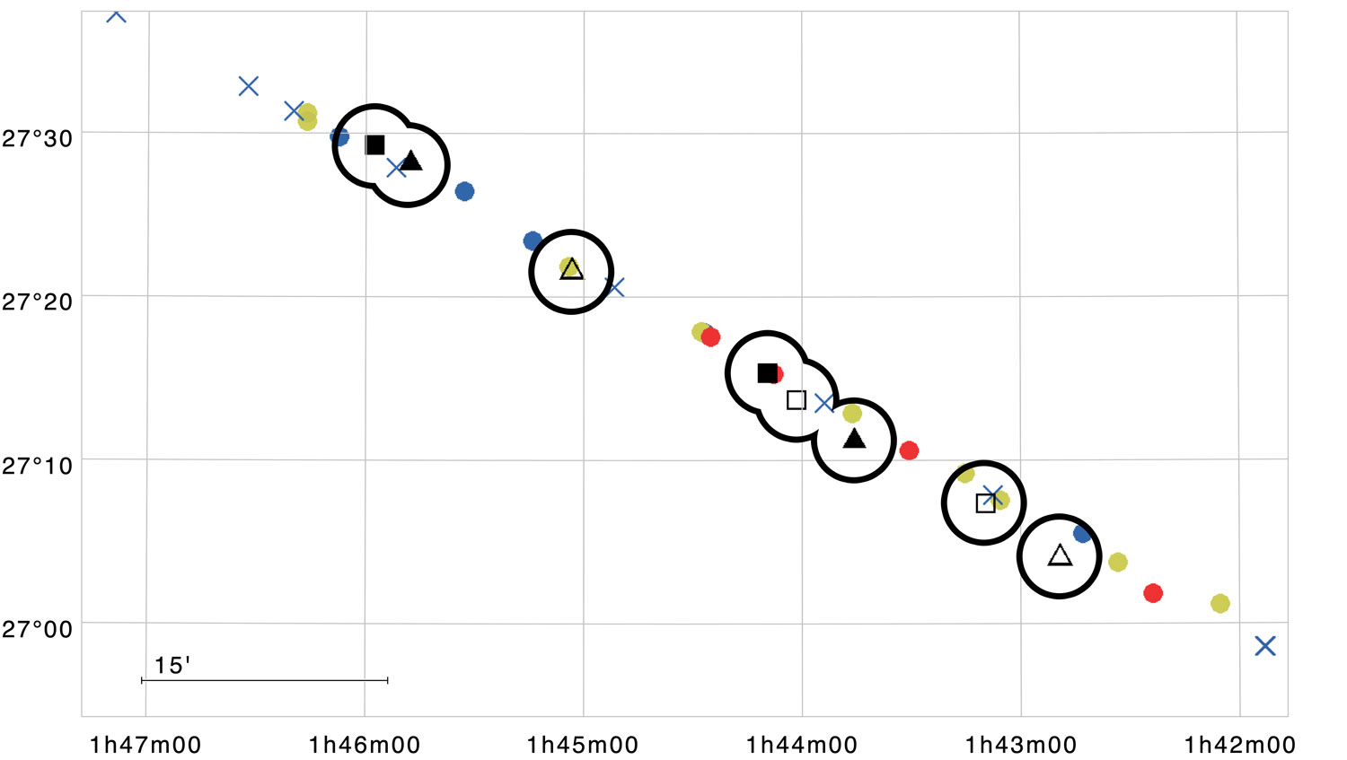
Figure 3: 17P Dust Trail kit model positions (markers with no circles as small, medium, big and toward the Sun particles) [1] and observations positions (square and triangle markers with circles) for dates 26.2. & 28.2.2022 and 1.3. & 2.3.2022. The X-axis shows RA and the Y-axis DEC. Model calculations M. Nissinen, M. Gritsevich, observations J. Ryske.
6. Summary and Conclusions
The particles released by the comet 17P/Holmes during the 2007 outburst formed a dust trail which is still possible to observe with relatively small aperture amateur sized telescopes using modern CCD-camera and image processing technology giving useful research data by amateur astronomers. Observations ensure that the developed dust particle model is producing the realistic results and can be used to forecast dynamics of meteoroid streams.
Acknowledgements
Special thanks to Arto Oksanen, Jyväskylän Sirius ry, image verification and Harry Lehto, University of Turku, image photometric guidance.
References
[1] Evolution of the Dust Trail of Comet 17P/Holmes, Maria Gritsevich, Markku Nissinen, Arto Oksanen, Jari Suomela, Elizabeth A. Silber. MNRAS Monthly Notices of the Royal Astronomical Society, 513(2), pp. 2201–2214, https://doi.org/10.1093/mnras/stac822
[2] Dust Trail Observations of Comet 17P/Holmes and Predictions for 2021-2022, Nissinen, Markku; Gritsevich, Maria; Oksanen, Arto; Suomela, Jari. Europlanet Science Congress 2021, EPSC2021-86.
How to cite: Ryske, J., Gritsevich, M., and Nissinen, M.: Validation of the Dust Trail kit model with the recent observations of the comet 17P/Holmes dust trail (February –March 2022), Europlanet Science Congress 2022, Granada, Spain, 18–23 Sep 2022, EPSC2022-60, https://doi.org/10.5194/epsc2022-60, 2022.
We present our preliminary results of searching for short-term variations of four long-period comets C/2016 M1 (PANSTARRS), C/2015 O1 (PANSTARRS), C/2014 W2 (PANSTARRS), C/2016 N4 (MASTER), and a hyperbolic comet C/2021 A1 (Leonard). All the comets reveal red color of their dust coma with slight variations, i.e., without changes of the color to blue or neutral. The observed dust productivity of the comets is quite high. Dust production respects to measurements of other long-period comets at the similar heliocentric distances. Comet C/2021 A1 (Leonard) was significantly redder comparing with the other comets and possessed weaker activity.
Introduction
In our research, we are looking for rapid variations of photometric color of comets at heliocentric distances beyond 3 au. The color reflects mainly the size distribution and also depends on the composition of dust particles (1; 2).
Variations of photometric color can be observed when we change the aperture size. It can be explained by differences in sizes and/or compositions of particles on different cometocentric distances, which can be caused by sublimation and/or fragmentation of dust particles (3; 4). On the second hand, except variations with the aperture size, the color was believed to be a constant characteristic of a cometary coma, but further studies have demonstrated changes of color during a long time (5; 6; 7). Furthermore, recent studies reveal much shorter variations of photometric color, i.e. days or months, which can be induced by changes of dust properties (3; 8; 9).
We analyze monitoring observations of 4 comets with highly eccentric elliptical orbits and a hyperbolic comet in order to find rapid color variations.
Observations
Observations of the comets were taken at the Skalnaté Pleso observatory (IAU Code – 056) using the 61-cm telescope. As CCD detector the FLI PL-230 camera have been taken. The pixel size of the camera is 15 µm, the field of view of 40.3 arcmin×40.6 arcmin, and the pixel scale was 1.18 arcsec/px. the Bessel B, V, R broadband filters were used. Images were taken without binning. During observations of comet C/2021 A1 (Leonard) in 2021 the telescope was equipped with the SBIG ST-10XME Dual CCD camera, having a pixel size of 6.8 µm, the field of view of 19.5 arcmin×13.1 arcmin and the pixel scale is 1.07 arcsec/px. We used a 2×2 binning mode. R and V filters of the Johnson-Cousins photometric system were used.
The reduction procedure (bias subtraction, dark and flat field corrections, and cleaning cosmic-ray tracks) was performed in in the standard manner, using the IDL routines (10; 8; 11). We used only photometric nights for analysis.
Results
At heliocentric distances bigger than 3 au, where the comets were observed, the coma is mostly formed by the sublimation of more volatile species, e.g., CO/CO2. Furthermore, at such distances gaseous emissions of daughter molecules are rarely observed in the optical region (12). Therefore, we assume that the observations obtained with the broadband filters allow us to study features of a dust coma.
We have not found significant variations of color from red to blue or neutral (or vice versa) in the selected comets. All the comets possessed red color of the dust coma with slight variations. Dust production of most long-period comets is similar to other comets of these family and is significantly bigger than for the Jupiter family comets. Only comet C/2016 N4 (PANSTARRS) has possessed lower activity.
Color of hyperbolic comet C/2021 A1 (Leonard) was usually bigger than for the other sampled comets, but dust production was on contrary smaller.
Acknowledgments
Our work was supported by the Slovak Grant Agency for Science VEGA No. 2/0059/22. Also, we were supported by the Slovak Research and Development Agency under the Contract no. APVV-19-0072.
References
1. Sen, A. K., et al. The effect of porosity of dust particles on polarization and color with special reference to comets. Journal of Quantitative Spectroscopy and Radiative Transfer. 2017, Vol. 198, pp. 164 - 178.
2. Jewitt, D. The active Centaurs. The Astronomical Journal. 2009, Vol. 137, 5, pp. 4296 - 4312.
3. Betzler, A. S., et al. An analysis of the BVRI colors of 22 active comets. Advances in Space Research. 2017, Vol. 60, pp. 612 - 625.
4. Farnham, T. L. Coma morphology of Jupiter-family comets. Planetary and Space Science. 2009, Vol. 57, pp. 1192-1217.
5. Jewitt, D. and Meech, K. J. Cometary Grain Scattering versus Wavelength, or, "What Color is Comet Dust?". Astrophysical Journal. 1986, Vol. 310, p. 937.
6. Li., J.-Y., et al. Constraining the Dust Coma Properties of Comet C/Siding Spring (2013 a1) at Large Heliocentric Distances. The Astronomical Journal Letters. 2014, Vol. 797, 1, p. 7.
7. Weiler, M., et al. The dust activity of comet C/1995 O1 (Hale-Bopp) between 3 AU and 13 AU from the Sun. Astronomy&Astrophysics. 2003, Vol. 403, pp. 313 - 322.
8. Ivanova, O., et al. Colour variations of Comet C/2013 UQ4 (Catalina). Monthly Notices of the Royal Astronomical Society. 2017, Vol. 469, 3, pp. 2695-2703.
9. Luk`yanyk, I., et al. Rapid variations of dust colour in comet 41P/Tuttle–Giacobini–Kresák. Monthly Notices of the Royal Astronomical Society. 2019, Vol. 485, 3, pp. 4013-4023.
10. Ivanova, O. V., et al. Photometric and spectroscopic analysis of comet 29P/Schwassmann-Wachmann 1 activity. Planetary and Space Science. 2016, Vol. 121, pp. 10-17.
11. Picazzio, E., et al. Comet 29P/Schwassmann-Wachmann 1 dust environment from. Icarus. 2019, Vol. 319, pp. 58-67.
12. Kulyk, I., et al. Physical activity of the selected nearly isotropic comets with perihelia at large heliocentric distance. Astronomy&Astrophysics. 2018, Vol. 611, p. A32.
How to cite: Voitko, A. and Ivanova, O.: Search for short-term color variations of five distant comets, Europlanet Science Congress 2022, Granada, Spain, 18–23 Sep 2022, EPSC2022-218, https://doi.org/10.5194/epsc2022-218, 2022.
Planetary community knows Ukraine as a country that has a prominent history of polarimetric studies of Solar system objects. Ukrainian planetary polarimetry has been counting since 1926 when academician M. Barabashov (Kharkiv) observed polarization of the Moon. It got a significant impetus in late 1950th since then concentrating in Kharkiv, Kyiv, and Crimea, and gradually moving its focus from polarimetric studies of Mars and Venus to comets and asteroids, at the same time keeping the leading role in the lunar polarimetry. In parallel with building polarimetric instrumentation and observing, Ukrainian polarimetric school also has had notable achievements in theory, specifically in studies of planetary and cometary atmospheres and surfaces of the Moon and asteroids, and in laboratory studies of light scattering by particulate surfaces. The devastating events of this year made it impossible for the Ukrainian polarimetrists to participate in the EPSC meeting. This poster intends to compensate for their absence by describing the history of the Ukrainian Polarimetric School and reminding the planetary community about leading Ukrainian polarimetrists and their contribution to the polarimetry of small bodies.
How to cite: Kolokolova, L., Sosonkin, M., and Levasseur-Regourd, A.-C.: Ukrainian School of Planetary Polarimetry, Europlanet Science Congress 2022, Granada, Spain, 18–23 Sep 2022, EPSC2022-263, https://doi.org/10.5194/epsc2022-263, 2022.
Background: Spectral observations in visual and near-infrared wavelengths are used to infer their surface material composition. Similar laboratory measurements of meteorites and various minerals and are used to link the known composition in laboratory measurements to asteroid composition.
However, many parameters in observations and measurements can introduce effects on the resulting spectra. With regolith-type powdered grains packed to a slab, the observing angles, particle size distribution, particle shapes, and space-weathering state of the material can all alter the spectra. Here, we try to model the particle size effects so that at least this effect could be understood when comparing different spectra.
Size effects in spectra: One can find spectral measurements of the same material but with varying size fractions in spectral databases such as RELAB (https://pds-speclib.rsl.wustl.edu/) and SSHADE (https://www.sshade.eu/). The typical spectral effects of different particle size are that the smaller particles are generally brighter, have redder slope, and deeper (absolute) absorption band depths. However, it is also possible to find counterexamples of different behavior.
Trend from light-scattering theory: If we limit to optically large particles (several times larger than the wavelength) and assume that different particle sizes are simply scaled versions of one particle, the particle size effects in spectra can be understood as interplay between surface reflections and absorption in the volume. If we assume that the surfaces are flat in the wavelength-scale, the surface reflections follow Fresnel reflections. For light that is refracted from the surface into the homogeneous material, the Beer-Lambert absorption gives the attenuation in the volume.
The Fresnel-type reflections do not absorb and are also only weakly dependent on the imaginary part k of the complex refractive index of the material, m=n+ik. The Beer-Lambert absorption, on the other hand, is only dependent on k and the distance traveled in the material, d. If the same volume is divided into smaller particles, typical d in the material between air-surface or surface-air interfaces and reflections or refractions from these is decreasing. Since absorption is taking place only in the volume, the increased surface reflections are increasing the brightness. This is the simple mechanism behind increasing brightness with decreasing particle size. At the same time, the exponent-term in the Beer-Lambert absorption affects so that similar change in d in the particle for a bright material has larger effect than the same d in darker material. This means that the absorption band depths are also increasing, in absolute units, when particle size is decreasing.
The possible increase of red slope with decreasing particle size in spectra cannot be explained with optically large particles. The longer wavelengths are ‘seeing’ the distances inside the particles shorter, but the effect is quite small for particles that are several times larger than the wavelength. However, if the sample also includes wavelength-scale particles, these are relatively more abundant in smaller size fractions and can introduce a red slope. This is because the scattering efficiency of particles increase when they reach wavelength-scale whereas for optically large particles it is constant.
Numerical modeling: We will verify and quantify the abovementioned theoretical trends with numerical simulations. We use a two-fold scheme where we first simulate the single-scattering properties (single-scattering albedo and the phase function) of individual random particle shapes, and then simulate the multiple-scattering effect in a packed slab of these particles.
We model the particles with a Voronoi cell particle model, see Fig. 1. In this model, a large volume is first filled with random seed points. Then, a 3d Voronoi division is done on the points, resulting the volume to be divided into Voronoi cells having flat surfaces and sharp corners. Finally, single cells are extracted from the volume, except the cells close to the edge of the volume to avoid edge-effects.

The light-scattering properties of single Voronoi particles are computed using a geometric-optics ray-tracing code SIRIS (https://bitbucket.org/planetarysystemresearch/siris4-framework/). These computations are run for 200 realizations of the particle model and changing the size parameter (physical size divided by the wavelength) and the real and imaginary parts of the refractive index. The results are averaged over the particle shape realizations.
The single-particle properties are fed into the Monte Carlo radiative transfer code RT-CB (https://bitbucket.org/planetarysystemresearch/rtcb_public/) where the amount of reflected light from a large slab containing the single particles is computed. This gives us the brightness as a function of particle size, wavelength, and real and imaginary parts of the refractive index.
Preliminary results: We have a grid of size parameters and refractive indices computed, and the results are consistent with what we expected from the simple theory of the changing ratio of surface reflections to volume absorption. We can, for example, plug in a typical behavior of the imaginary part of olivine as a function of wavelength, keep the real part of the refractive index constant for simplicity (it does not change much in visual/near-infrared wavelengths), and plot the spectra of different-sized olivine particles, see Fig. 2.

Conclusions and future work: Currently, we are increasing the parameter grid to include both smaller size parameters and smaller imaginary k values. From the results we have, it seems that we can fit an analytical function to the results with quite small prediction errors. If successful, this analytical model can be used to model the size effect on the reflectance spectra of particulate materials if the particles are clearly larger than the wavelength. If we can model, we can also remove the effect if we know the particle sizes and receive size-standardized spectra that can be better compared between the samples.
As a side product, we can use this data and the model to invert the imaginary part of the refractive index for materials from which we have reflectance spectra measurements and the particle size.
How to cite: Penttilä, A., Martikainen, J., and Muinonen, K.: Modeling the effect of particle size distribution on spectra for optically large particles, Europlanet Science Congress 2022, Granada, Spain, 18–23 Sep 2022, EPSC2022-415, https://doi.org/10.5194/epsc2022-415, 2022.
Introduction: DART mission will be the first to undertake an orbital deflection experiment against a Near-Earth Asteroid. The smallest member of the binary Didymos-Dimorphos system will be impacted by the 660-kg spacecraft at the velocity of 6.6 km/s, leading the orbital period to change in return. The expected baseline kinetic energy is 9.7 GJ [1], about half the input energy of Deep Impact[2], and >10^5 kg of mass is to be released [3].
The impact will produce an ejecta plume, lasting for several minutes [3], that will be observed by ASI/LICIACube camera up to about 4 m/px resolution [4,5] and phase angles ranging from 45 to 120 deg. The plume is therefore expected to be resolved during several frames and its phase function studied in order to retrieve properties such as albedo, grain size frequency distribution and optical depth. Therefore, we put forth a light scattering model that relies on previous knowledge about the Dydimos binary system composition [6] and the Deep Impact event [7].
LICIACube Observations: The Light Italian Cubesat For Imaging Asteroids is a 6C Cubesat hosted by DART spacecraft. LICIACube will detach from DART spacecraft 10 days from the nominal impact date of 26th September 2022 to start the trajectory correction to be positioned in fly-by mode. LICIACube payload holds two optical cameras, LUKE and LEIA, designed for color imaging studies [5]. At 167 sec after the impact, the Italian Cubesat will reach the closest approach and obtain the highest resolution images from the binary system.
Methodology: grain size range. To provide support and analyze the broad grain’s size distribution range expected in the plume, we relied two numerical codes covering two different size regimes: (i) The Mishchenko et al., [8,9] radiative transfer code for Mie-Lorentz scatters distribution (~0.5-80 microns size in visible range) with Percus-Yevick filling factor correction (called RTT-PM, [10]) to model the thick portion of the plume; (ii) and the Muinonen et al. [11] ray optics code for diverse particle shapes and sizes higher than 100 microns.
model conditions. The plume boundaries are considered much similar to an atmospheric cloud, with particles sparse, many mean radii separated from each other, and the observations in far-field, removed several kilometers from the object of study. Furthermore, we imposed that the number of large particles (>100 microns) is much smaller than the number of Mie-Lorenz particles, therefore limiting the interactions among the large particles, but not with the small particles. Hence, the validity regime for the radiative transfer equation is conserved. Furthermore, coherent effects, shadowing, and opposition effect mechanisms are out of the scope of our calculations and observational conditions with LICIACube.
interaction. The interactions are only resolved between the thick cloud and the >100 microns particles. In the first approach, we compute the particles hovering over the radiative transfer semi-infinite plane of the thick plume, as it gets backlit in varied distances up. In reverse, the thick plume is forward-lit by the particle scattering. In the second approach, the large particles are embedded in the thick plume up to optical depth = 5, again, the medium is considered sparse.
Preliminary Results: Given that Didymos is an S-type asteroid, with visible spectra profile very similar to L/LL Chondrites [6], we selected the Itokawa sample size frequency distribution obtained by the Hayabusa mission as analog [12]. L/LL Chondrite most abundant minerals are Fayalites and Ferrosilites. However only VIS optical constants for Fayalites were recovered [13], thus we stick with it in our simulations. In Fig. 1, we present the bi-directional reflectance distribution factor (BRDF) for the layers composing the plume in our simulation: (I) thick “core”, multiple-scattering Mie RTT-PM; (ii) “scattered small particles'', single-scattering-only Mie-Lorenz particle volumes; (iii) “scattered large particles”, single-scattering-only >100 microns particle volumes. The BDRF can therefore vary as the volumes become less opaque, leading to less reflectiveness for middle phase angles.
In future developments of our modeling, we will use results from ejecta dynamics to constrain the number of particles and population for different zones and lines of sights through the plume [14, 15, 16].
Furthermore, the interaction of the large particles and the thick Mie particle cloud is under refinement, as we test the codes for different binning, distances and depths. Nonetheless, first tests indicate a magnification of the overall BRDF for large azimuth angles, due to coupling with the overall forward scattering behavior of the large particles.
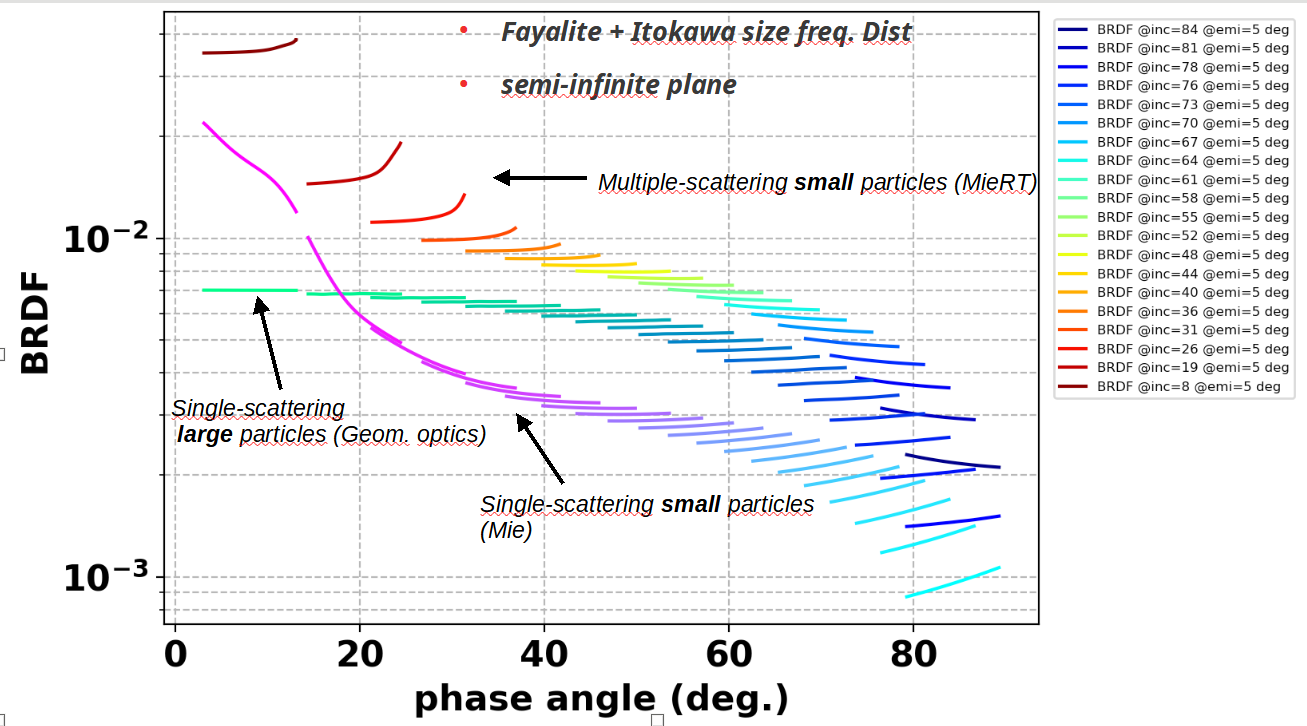
Fig. 1. bi-directional reflectance distribution factor for different layers of the plume, separately. Fayalite’s optical constants at 550 nm (Re(m)=1.6, Im(m)=5e-3) are used, together with Itokawa sample size frequency distribution (Nakamura et al., 2012). Filling factor for RTT-PM is fixed at 0.1%.
Acknowledgements: This research was supported by the Italian Space Agency (ASI) within the LICIACube project (ASI-INAF agreement AC n. 2019-31-HH.0).
References: [1] Sarli et al., 2017, AAS/AIAA 17-206.[2] Groussin et al., 2010, Icarus 205, 627–637.[3] Cheng et al., 2020, Icarus 352, 113989.[4] Dotto et al., 2021, PSS, Volume 199, 10518.[5] Poggiali et al., 2022, PSJ Focus Issue (submitted).[6] Ieva et al., 2022, PSJ Focus Issue (submitted).[7] A’Hearn, 2006, 229th IAU Sym. ACM Proc., 33-40.[8] Mishchenko et al., 1999, JQSRT, 63, 409-432.[9] Mishchenko et al., 2015, JQSRT 156, 97-108.[10] Ito et al;, 2018, JGRE 123, 5, 1203-1220[11] Muinonen et al., 2009, JQSRT 110, 14-16, 1628-1639.[12] Metzger & Britt, 2020, Icarus 350, 113904.[13] Fabian et al., 2001, A&A 373, 1125–1138.[14] Rossi, A. F. et al., 2022, PSJ, Focus Issue (in press).[15] Zanotti, G., and M. Lavagna, 2020, IAC 71.[16] Ivanovski et al., 2022, PSJ Focus Issue (submitted).
How to cite: Hasselmann, P. H., Bertini, I., Zanotti, G., Rossi, A., Ivanovski, S., Gai, I., Deshapriya, J. D. P., Mazzotta Epifani, E., Dotto, E., Della Corte, V., and Zinzi, A. and the LICIACube Team: DART mission ejecta plume: Modeling the reflectance through radiative transfer and geometric optics in support to LICIACube observations, Europlanet Science Congress 2022, Granada, Spain, 18–23 Sep 2022, EPSC2022-615, https://doi.org/10.5194/epsc2022-615, 2022.
SB6 | Cosmic Dust in our Solar System
In our solar system, meteoritical matter exhibits a variety in bulk compositions that is representative of the processing history of refractory matter in the protosolar nebula (PSN). This history is usually investigated via a thermodynamic approach, where refractory grains condense out from a hot cloud. However, in the innermost regions of the PSN the migration timescale of grains can exceed the evaporation timescale of refractory species.
We investigate the role played by rocklines (condensation/sublimation lines of refractory materials) in the innermost regions of the PSN to compute the composition of drifting and evaporating grains. To do so, we compute the evolution of the PSN using a 1D viscous accretion disk model [1]. The disk is initially filled with dust that is a mixture of several refractory species of protosolar composition. This dust exists in the form of refractory grains and their vapors. The radial transport of grains is computed by solving an advection-diffusion equation, and phase transitions are accounted for by computing sublimation and condensation rates for each species. We then compare the composition of the PSN computed by our model with the composition of meteoritical bodies collected on Earth.
We find that the compositional gradient in the PSN that is created by rocklines, shown in Figures 1 and 2, matches the composition of cosmic spherules, chondrules, and chondrites. Moreover, our model shows that solid matter is concentrated in the vicinity of these sublimation/condensation fronts. Although our model only focuses on the most abundant refractory species (olivine, represented in our model by its end members forsterite and fayalite; enstatite and ferrosilite pyroxenes; kamacite and taenite metal; and iron sulfide), it suggests that rocklines heavily processed refractory matter in the PSN, which has important consequences for the composition of small and large bodies in the innermost regions of the solar system. The local increase of the iron abundance close to rocklines of iron alloys could have contributed to the high Fe-content in Mercury.
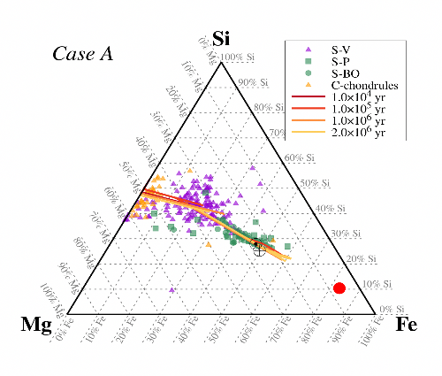
Figure 1. Composition profiles of the PSN in a Mg-Fe-Si ternary diagram (expressed in mass fraction) at different times, with composition of glass cosmic spherules (S–V type), barred olivine spherules (S-BO type), porphyritic spherules (S-P type) and C-chondrules. Protosolar and Earth’s compositions are represented by Sun’s and Earth’s symbols, respectively, and Mercury’s composition is represented by a red circle.
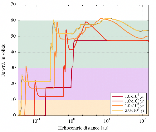
Figure 2. Same as Figure 1, but here the Fe wt% is represented as a function of heliocentric distance. Color boxes correspond to typical compositions of chondrules (0%–10%), glass cosmic spherules (10%–30%), and porphyritic and barred olivine cosmic spherules (30%–60%).
[1] Aguichine, A., Mousis, O., Devouard, B., and Ronnet, T. 2020, ApJ, 901, 97.
How to cite: Aguichine, A., Mousis, O., and Devouard, B.: Processing of refractory species in the vicinity of rocklines, Europlanet Science Congress 2022, Granada, Spain, 18–23 Sep 2022, EPSC2022-358, https://doi.org/10.5194/epsc2022-358, 2022.
SB7 | Laboratory measurements of returned Hayabusa2 samples, meteorites and planetary analogues
Introduction
Astrophysical ices were observed in various environments with different compositions : from the icy grains of the interstellar medium (ISM, [1]), to various bodies of the solar system such in icy moons of Jupiter or Saturn systems, or in comets. In such environments, ice is subjected to various alterations ranging from a wide range of UV doses, different physicochemical alterations [2], thermal alterations [3] and various primitive ice composition [4]. As inferred by laboratory experiments, these ice alterations are now known to generate a large molecular diversity ( [5], [6]). This organic matter is well observed in certain meteorites where up to 4 % of the total matter is organic (carbonaceous chondrites [7]), but this number can grow up to 45 % in interstellar dust particles and comets [8]. Laboratory experiments suggest that grain chemistry from primitive ices composed of H2O, NH3, methanol (MeOH) or other molecules is the main source of this astrophysical organic matter ([9], [10]). The reactivity occurring during the alteration of such an ice is a two step mechanism: First, energetic processes form radicals such as H•CO or •CH2OH which directly produces molecules such as CO or CO2 [14]; Then, thermal reactivity can occur to form more complex organic compounds. During this second phase, radicals diffuse, which allows their recombination forming more complex molecules such as hexamethylenetetramine (HMT), polyethyleneimine (PMI) or polyoxymethylene (POM) [15].
The refractory [16] and volatile [17] compositions of the final organic pool is thus highly influenced by the initial ice composition ratio. In the present work, we investigate the influence of the heating rate, the residual pressure or of the photon/molecule ratio on this final organics.
Method
All the experiments were monitored in the MICMOC experiment already described in [11]. It is a cryogenic vacuum chamber (~10-7 mbar) with a finger cooled down up to 77 K using liquid nitrogen. The cold finger contains IR transparent MgF2 windows on which primitive moieties H2O, NH3 and methanol (MeOH) are deposited within a fixed 3:1:2 ratio (H2O:MeOH:NH3). The irradiation at Lyman α (121 nm) is concomitant to the ice formation during 70 h and then warmed up to ~300 K. The following experiments were performed :
- Various irradiation rates (1,5.103, 141, 5 photon/MeOH), by modifying the flux of matter;
- Fixed irradiation (~80 photon/MeOH) and various heating rates (0.5, 4, 8 K/min) monitored by a heating resistance after the irradiation phase;
- Fixed irradiation and various pressures of Ar added during the heating phase.
All samples were then analyzed using both fourier-transform infrared spectrometry (FT-IR) and electrospray fourier- transform ion cyclotron resonance mass spectrometry (ESI-FT-ICR [18]).
Preliminary results and conclusions
Preliminary results are displayed Figure 1. First, infrared spectroscopy measurements show weak impacts of heating rate and residual pressure during the warming phase: The main IR features present similar intensities implying no significant evolution of the final organic products. The only significant influence observed is the lower FT-IR intensity recorded at lower heating rate (0.5 K/min). Regarding the irradiation rate, it shows the highest evolution on the IR signatures : for low irradiation rates (5 photon/MeOH) ν(OH) at 3242 cm-1 vs νas(CH) at 2923 cm-1 ratio is significatively modified and ω(CH2) at 1458 cm-1 and νas(COO-) at 1598 cm-1 are significatively exhausted. This suggests the presence of salts, polyoxymethylene (POM), hexamethylenetetramine (HMT) and polyethyleneimine (PMI) in higher quantities in this sample. On the contrary, the FT-IR spectrum of the higher irradiated sample shows no features because of a decrease in the yield of organic production implying a lack of sensitivity with FT-IR.
To obtain complementary information on the molecular evolution ESI-FT-ICR analysis was recorded on the same samples. The ESI-FT-ICR confirmed the preliminary results observed with FT-IR with a better insight on the molecular processes impacting the final organic composition. All together the influence of those three parameters are the following :
- Irradiation has a high impact on the molecular content of the sample, mostly on the DBE, but also on the molecular diversity and abundance;
- The increase of the residual pressure during the heating phase has a weak influence, even if it increases a higher experimental dispersion regarding the molecular abundance while the molecular diversity is not impacted;
- Finally, the heating rate has a very weak influence on the final organic composition.

Figure 1 Comparison of FT-IR spectra or ESI+ FT-ICR mass spectra of the residue for each sample series (A, B, C). Global shape of both ESI+ and ESI– of FT-ICR analysis are showing similar properties.
Bibliography :
[1] D. H. Wooden et al., “Composition and Evolution of Interstellar Clouds,” in Comets II, University of Arizona Press, pp. 33–66, 2004.
[2] G. M. Muñoz Caro et al., ACS Earth Space Chem, vol. 3, no. 10, pp. 2138–2157, 2019.
[3] O. Mousis et al., Astrophys. J., vol. 819, no. 2, p. L33, 2016.
[4] M. J. Mumma and S. B. Charnley, Annu. Rev. Astron. Astrophys., vol. 49, no. 1, pp. 471–524, 2011.
[5] G. Danger et al., GCA, vol. 118, pp. 184–201, 2013.
[6] A. Ruf et al., Life, vol. 9, no. 2, p. 35, 2019.
[7] S. Pizzarello and E. Shock, Cold Spring Harb. Perspect. Biol., vol. 2, no. 3, pp. a002105–a002105, 2010.
[8] J.-L. Bertaux and R. Lallement, MNRAS, vol. 469, no. Suppl_2, pp. S646–S660, 2017.
[9] A. Gutiérrez-Quintanilla et al., MNRAS, vol. 506, no. 3, pp. 3734–3750, 2021.
[10] G. Fedoseev et al., MNRAS, vol. 448, no. 2, pp. 1288–1297, 2015.
[11] L. d’Hendecourt and E. Dartois, Spectrochim. Acta A Mol. Biomol. Spectrosc., vol. 57, no. 4, pp. 669–684, Mar. 2001.
[12] P. Schmitt-Kopplin et al., PNAS, vol. 107, no. 7, pp. 2763–2768, 2010.
[13] F. Duvernay et al., ApJ, vol. 791, no. 2, p. 75, 2014.
[14] K. I. Öberg, Chem. Rev., vol. 116, no. 17, pp. 9631–9663, 2016.
[15] V. Vinogradoff et al., A&A, vol. 551, p. A128, 2013.
[16] A. Fresneau et al., ApJ, vol. 837, no. 2, p. 168, 2017.
[17] N. Abou Mrad et al., ApJ, vol. 846, no. 2, p. 124, 2017.
[18] P. Schmitt-Kopplin et al., Anal. Chem., vol. 82, no. 19, pp. 8017–8026, 2010.
How to cite: Javelle, T., Ruf, A., Schmitt-Kopplin, P., and Danger, G.: Impacts of residual pressure, heating rate and photon to molecular ratio on the molecular composition generated by the processing of astrophysical ices, Europlanet Science Congress 2022, Granada, Spain, 18–23 Sep 2022, EPSC2022-102, https://doi.org/10.5194/epsc2022-102, 2022.
Micro- and nano-scale computed tomography (µ-CT, n-CT) is a relatively fast method for studying, among others, textural and physical properties of solid materials. For example, we are using micro- and nano-CT techniques to study chondrules and CAIs from primitive meteorites. If properly calibrated, CT studies can also help obtaining (qualitative) chemical information. However, there was always the question whether or not CT-techniques are non-destructive. We tested for this by using matrix material from the CV3 chondrite Allende. We prepared a powdered matrix sample and divided them into five aliquots; three aliquots were irradiated using a Bruker SkyScan 1272 µXCT-Scanner, at the Anatomy department at the university of Bern, operating at 70 keV, 50 keV, or 30 keV. Two samples served as non-irradiated standards. We investigated if the irradiation has any effect on the noble gas concentrations. We found that that there is no effect, i.e., the noble gas concentrations are indistinguishable between irradiated and non-irradiated samples. Since there is no effect for the very fine-grained matrix material, we can conclude that there is also no effect for larger objects like chondrules and CAIs.
How to cite: Ghaznavi, P., Kadlag, Y., Leya, I., and Haberthuer, D.: The effects of irradiation on the noble gases in matrix of Allende (CV) meteorite, Europlanet Science Congress 2022, Granada, Spain, 18–23 Sep 2022, EPSC2022-115, https://doi.org/10.5194/epsc2022-115, 2022.
- Introduction
The characterization of the complex magnetic susceptibility (real and imaginary parts) of rocks is an unexplored tool to constrain the composition, structure and geological history of rocks in surface planetary exploration. We propose the NEWTON susceptometer for the determination of the complex magnetic susceptibility, to provide valuable information about the regolith and surface rocks in rocky bodies of the solar system, to be used as a selection criterion of rocks for sample return missions or for the in-situ scientific studies of the magnetic properties during planetary missions [1]. The instrument is based on AC - inductive methods, and its dynamic range of the real susceptibility covers magnetic susceptibility values for rocks from the Earth, Moon and Mars [2, 3, 4]. The sensor is suitable to be placed on board rovers, or to be used as a portable device during field campaigns and by astronauts in manned space missions. This sensor provides a great advantage compared to available commercial susceptometers due to its robustness, compatibility with the planetary environments and that it does not require sample preparation, but only minimum sample dimensions (~50 x 20 x 20 mm).
The aim of this work is to test the capability of the instrument in two different scenarios with distinct types of samples representative of a wide susceptibility range: 1) the in-situ real magnetic susceptibility determination in Cerro Gordo volcano, considered as a terrestrial analogue [5]; and 2) the characterization of meteorites from the collection of the Museo Geominero (Madrid, Spain).
The first study case consists of an intraplate volcano, with potential similar composition and structure of volcanoes from Mars. The second study case comprises various meteorite samples of different origins.
2.1 Terrestrial analogue: Cerro Gordo volcano
Cerro Gordo volcano was proposed as a Martian analogue due to its structural similarities with Martian volcanoes. It lies to the SW of Almagro (38°49’13”N/3°44’37”W), within the Campo de Calatrava volcanic region in Spain [6], and is emplaced among Paleozoic host rocks where the Armorican quartzite yields the topographic heights.
Cerro Gordo is part of a volcanic lineation, all of olivinic nefelinite composition and thought to have erupted coevally (1.5 ± 0.3 Ma [7]), that follows a NNE-SSW fracture [8]. Its eruptive style varied with time from phreatomagmatic to strombolian and phreatomagmatic again to end with an effusive phase [9]. For this reason the deposits found in the field (pyroclastic surge deposits, lahar facies, scoria and pyroclastic deposits, a lava flow, tuffs, breccias and spatter deposits) are varied in composition and structure, and therefore comprise a large range of magnetic susceptibility values, making Cerro Gordo an excellent scenario for a demonstration campaign of the susceptometer prototype.
2.2 Meteorites
A total of 16 meteorites of different compositions, and therefore varied susceptibility ranges, have been measured for this work, 10 aerolites and 6 siderites. The criteria followed was that their volume accomplished the minimum size stated in the introduction. The samples were divided into faces and measured twice in each of them. In the case of the siderites showing a flat polished face with Widmanstätten structures, the polished face was measured in two orthogonal directions to test the possible influence of the internal structural ordering.
- Conclusions
Previous results from Cerro Gordo showed the capability of the magnetic susceptibility results to distinguish between different rock deposits. The ongoing work on the collected samples analysis and geological description of the study location is intended to relate the magnetic susceptibility values with the mineral composition of the rocks, enhancing the comprehension of the susceptibility measurements and the structure of the volcano. The measurements on meteorites are currently under analysis, and aim to classify the measured samples as a function of their magnetic susceptibility [10].
Acknowledgements:
This work has been funded by the Spanish Programme for Research, Development and Innovation under the grants of references ESP2017-88930-R and PID2020-119208RB-I00: MagAres and MINOTAUR, respectively, as well as the European Union Project NEWTON, of grant agreement 730041. JSO is funded by the European Union’s Horizon 2020 research and innovation programme under the Marie Sklodowska-Curie grant agreement SIGMA no 893304.
References:
[1] Díaz Michelena et al. 2017, Sensor Actuat A-Phys, vol. 263, pp. 471-479
[2] Rochette et al. 2005, Meteoritic and Planetary Science, 40 (4): 529–540
[3] Rochette 2010, Earth Planet. Sci. Lett., 292: 383–391.
[4] Hunt et al. 2013, Wiley. Online Library. DOI: 10.1029/RF003p0189.
[5] Monasterio et al. 2021, Terrestrial Analogs Conference (LPI Contrib. No. 2595)
[6] Becerra-Ramírez et al. 2020, Geosciences, 10, 441.
[7] Ancoechea & Huertas 2021, J. Iberian Geology (47): 209-223.
[8] Ancoechea 1999, Enseñanza de las Ciencias de la Tierra (73): 237-243.
[9] González et al. 2010, Aportaciones Recientes en Volcanología 2005-2008: 57-65.
[10] Rochette et al. 2003, Meteoritics & Planet. Sci., 38: 251-268.
How to cite: Mesa Uña, J. L., Losantos, E., Oliveira, J. S., G. Monasterio, Ó., and Díaz Michelena, M.: Testing the applicability of NEWTON Susceptometer for fast and in-situ determination of the magnetic susceptibility, in meteorite samples and a Martian terrestrial analogue., Europlanet Science Congress 2022, Granada, Spain, 18–23 Sep 2022, EPSC2022-827, https://doi.org/10.5194/epsc2022-827, 2022.
Introduction
Comets are the most primitive bodies of the solar system [1]. They are composed of low density material: mainly dust and ice. A better understanding of their composition is of particular interest to improve the comprehension of the composition of the material composing the forming solar system. Nevertheless, because of detection issues, the composition of its nucleus is only poorly known even eight years after the landing of the Philae probe from the European Space Agency (ESA) Rosetta mission. Most insights on the organic composition of 67P/Churyumov-Gerasimenko are coming from indirect analysis estimating that around 45 % of a comet is composed of organic matter ([2],[3]).
Laboratory experiments show similarities with the organic matter observed in comets [4]. Astrochemical experiments are thus a promising approach to cover this lack of data. Experiments simulating the chemical reactivity occurring on icy grains initially composed with volatile molecules such as H2O, NH3, methanol (MeOH) give information into the refractory [5] and volatile [6] organic composition that are formed in such astrophysical environments. Those experiments suggest the presence of a large organic diversity [7]. Previous work showed the correlation between the initial composition of these ices and either the volatile organic compounds (VOCs) composition [8] or the refractory organic material [9]. In this presentation, we will give the first experimental description of the correlations that exist between both three phases: the primitive ice composition, the refractory and the gas phase.
Method
All samples were synthesized using the MICMOC experiment [10]. It is a vacuum chamber (~10-7 mbar) where different ice compositions of H2O, NH3 and methanol (MeOH) were irradiated at Lyman α (121 nm) at 77 K for 5,5 h at a fixed irradiation rate of ~7 photon/MeOH. Then, 92 mbar of argon were added before the sample was warmed up to ~300 K. Four ice compositions were tested : a benchmark experiment (Ref.) with ratio 3:1:2 (H2O:MeOH:NH3); a H2O-rich sample, 8:1:2; a NH3-rich sample, 2:1:5; and a MeOH-rich sample, 2:5:3.
VOCs are recovered using an extra cryogenic trap coupled to a valve system for GC-EI-FT-Orbitrap analysis [11]. Three replicates are made for each ice composition. The cumulation of the three residual phases from all samples is then extracted and dissolved 10 times into methanol before positive ESI-FT-ICR. More details on the apparatus characteristics can be found in [12].
To extract correlations between all three phases (initial ice, refractory and gas), principal component analysis (PCA) were performed on the dataset standardized by variable with following characteristics :
- For the gas phase (Figure 1A): individuals are the triplicates of GC-EI-FT-Orbitrap analysis with 150 chromatographic peak areas as variables;
- For the refractory phase (Figure 1B): individuals are the analysis of methanol solubilized refractory material injected using positive ESI-FT-ICR with between 4126 to 12814 extracted exact mass peak area as variables.
Preliminary results and conclusions
PCA is a mathematical tool to find the smartest plan to differentiate individuals in a multiple variable hyperspace. Figure 1 displays the plan with highest differences from those two datasets. Axes 1 and 2 are mostly enough to discriminate samples according to their initial composition for both gas phase (Figure 1A) and residual phase (Figure 1B). As most individual ices are present in different zones, it proves the organic composition of each phase allows to find correlation between them.
More specifically, in the gas phase (Figure 1A) only three zones can be determined : the first one contains only NH3-rich ices, the second one MeOH-rich ices and the third one both the benchmark experiment (Ref.) and H2O-rich ices. Consequently, H2O, NH3 and MeOH seem to have different impacts on the volatile organic compounds: H2O seems to be less impactful on the first and second principal axes while only the third axes can discriminate it from the other zones.
Finally, all three parameters can be separated using ACP on residual phase, proving significant differences extracted from the intensity and compound nature detected by positive ESI-FT-ICR. All together, this suggests a high correlation between all three phases regarding their organic compound composition.
Shortly :
- On the gas phase : NH3 hinders all volatile productions including nitriles, H2O has little impact on the gas composition with respect to the benchmark experiment.
- On the refractory phase : NH3 and H2O are changing the nature of organics produced and making global ESI-FT-ICR intensity. H2O is the ice that’s producing the smaller organic diversity (tree time less compounds detected).
- In both gas and residual phase : MeOH has little impact on the final organic compound type, but enhances the total amount of them.
A) |
B) |


Figure 1. Principal component analysis (PCA) of results from each sample. In A) individuals are the triplicates of GC-EI-FT-Orbitrap analysis with chromatographic peak areas as variables. In B) individuals are each four analyses of methanol solubilized refractory material injected using positive ESI-FT-ICR with exact mass peak area as variables. Samples are labeled according to the compound exhausted in the initial composition of the ice with respect to the benchmark experiment (Ref.); H2O for the H2O-enriched sample; NH3 for the NH3-enriched sample and a MeOH for the MeOH-enriched sample.
Bibliography :
[1] M. J. Mumma and S. B. Charnley, Annu. Rev. Astron. Astrophys., vol. 49, no. 1, pp. 471–524, 2011.
[2] J.-L. Bertaux and R. Lallement, MNRAS, vol. 469, no. Suppl_2, pp. S646–S660, 2017.
[3] K. Varmuza et al., J Chemom, vol. 34, no. 4, 2020.
[4] F. Duvernay et al., ApJ, vol. 791, no. 2, p. 75, 2014.
[5] G. Danger et al., GCA, vol. 118, pp. 184–201, 2013.
[6] N. Abou Mrad et al., Anal. Chem., vol. 86, no. 16, pp. 8391–8399, 2014.
[7] A. Ruf et al., Life, vol. 9, no. 2, p. 35, 2019.
[8] N. Abou Mrad et al., ApJ, vol. 846, no. 2, p. 124, 2017.
[9] A. Fresneau et al., ApJ, vol. 837, no. 2, p. 168, 2017.
[10] L. d’Hendecourt and E. Dartois, Spectrochim. Acta A Mol. Biomol. Spectrosc., vol. 57, no. 4, pp. 669–684, Mar. 2001.
[11] T. Javelle et al., J. Chromatogr. A, vol. 1652, p. 462343, 2021.
[12] P. Schmitt-Kopplin et al., Anal. Chem., vol. 82, no. 19, pp. 8017–8026, 2010.
How to cite: Javelle, T., Schmitt-Kopplin, P., and Danger, G.: Correlations between cometary ice composition and their refractory and gas organic diversity: clues from laboratory experiments, Europlanet Science Congress 2022, Granada, Spain, 18–23 Sep 2022, EPSC2022-1018, https://doi.org/10.5194/epsc2022-1018, 2022.
Introduction: Primitive asteroids that accreted beyond the snowline in the protoplanetary disk likely played a crucial role in the delivery of water and organic matter to Earth and other terrestrial planets. The surface of the Cb-type asteroid 162173 Ryugu has low overall reflectance and an absorption feature at ~2.7 µm consistent with the presence of carbonaceous materials and phyllosilicates [1]. The spectral characteristics of Ryugu’s surface are most similar to the highly altered CI (“Ivuna-like”) and/or dehydrated CY (“Yamato-like”) carbonaceous chondrites [2].
In December 2020, JAXA’s Hayabusa2 mission successfully returned to Earth with >5 g of sample collected from the surface of Ryugu. The initial investigation of the samples suggested a close affinity with the CI chondrites [3], which consist of abundant phyllosilicates (~80 vol.%), plus minor amounts of magnetite (~10 vol.%), and dolomite (<5 vol.%), having experienced low temperature (<100°C) aqueous alteration [4]. In contrast, the CY chondrites contain dehydrated phyllosilicates and/or recrystallized olivine (~70 vol.%), Fe-sulphides (up to ~20 vol.%), and sometimes metal (~1 vol.%) following post-hydration metamorphism at temperatures >500°C [5]. Here, as part of the Hayabusa2 “Stone” preliminary examination team, we have characterised the modal mineralogy of a Ryugu particle to further constrain its aqueous and thermal history.
Methods: A powdered sub-sample of Ryugu particle C0002 (plates 3 and 4) was analysed using position-sensitive-detector X-ray diffraction (PSD-XRD) at the Natural History Museum (NHM), London. XRD patterns were acquired from the Ryugu powder using a high-intensity micro X-ray source for 6 hours, with the sample rotated throughout the analysis. Pure standards of each phase detected in the Ryugu powder were analysed under exactly the same conditions for 15 minutes. The modal mineralogy of the Ryugu powder was then determined using an established peak fitting method [4, 5].
Results & Discussion: Ryugu particle C0002 (plates 3 and 4) contains a mixture of Mg-rich serpentines and smectites that are present at an abundance of ~84 (± 2) vol.%. Other phases identified from the XRD pattern include magnetite (~8 vol.%), pyrrhotite (~7 vol.%), and dolomite (~2 vol.%). This mineralogy is broadly consistent with our petrographic observations of polished Ryugu sections (C0025-01 and C0103-02). Diffraction peaks from anhydrous olivine and pyroxene were not observed suggesting that their abundance is ≤1 vol.% in the analysed fraction of C0002. If we assume a maximum anhydrous silicate abundance of 2 vol.%, then the phyllosilicate fraction (PSF = total phyllosilicate abundance / [total anhydrous silicate + total phyllosilicate abundance]) of the Ryugu powder is 0.98, which corresponds to a petrologic sub-type of 1.1 on the alteration scale of Howard et al. [6].
The XRD pattern and modal mineralogy of Ryugu particle C0002 (plates 3 and 4) is very similar to the CI chondrites [4]. However, the Ryugu powder does not contain sulphates and ferrihydrite, which are common in the CI chondrites and thought to be terrestrial weathering products [7]. The Ryugu powder also has a comparable mineralogy to the recent C2ung fall Tarda, which appears to be related to the Tagish Lake (C2ung) meteorite [8]. However, Tarda retains partially altered chondrules and has a relatively high abundance of anhydrous silicates (~10 vol.%) [9]. In addition, the XRD pattern and modal mineralogy of the Ryugu powder is clearly distinct from the CY chondrites, which contain dehydrated phyllosilicates that lack coherent diffraction, and abundant poorly crystalline troilite and secondary olivine [5].
The modal mineralogy of Ryugu particle C0002 (plates 3 and 4) is consistent with having formed through low temperature aqueous alteration. The fluid-rock reactions reached near-completion, resulting in a secondary assemblage of phyllosilicate, sulphide, magnetite, and Mg-carbonate that was not overprinted by a later episode of thermal metamorphism at temperatures >~400°C.
References: [1] Kitazato et al. (2019) Science. 364:272. [2] Kitazato et al. (2021) Nature Astronomy. 5:246. [3] Yada et al. (2022) Nature Astronomy. 6:214. [4] King et al. (2015) Geochimica et Cosmochimica Acta. 165:148. [5] King et al. (2019) Geochemistry. 79:125531. [6] Howard et al. (2015) Geochimica et Cosmochimica Acta. 149:206. [7] Gounelle & Zolensky (2001) Meteoritics & Planetary Science. 36:1321. [8] Marrocchi et al. (2021) The Astrophysical Journal Letters 913:L9. [9] King et al. (2021) 52nd LPSC, abstract #1909.
How to cite: King, A., Russell, S., Nakamura, T., Yurimoto, H., Noguchi, T., Okazaki, R., Yabuta, H., Naraoka, H., Sakamoto, K., Tachibana, S., Watanabe, S., and Tsuda, Y.: The modal mineralogy of asteroid 162173 Ryugu and its relationship to carbonaceous chondrite meteorites, Europlanet Science Congress 2022, Granada, Spain, 18–23 Sep 2022, EPSC2022-1264, https://doi.org/10.5194/epsc2022-1264, 2022.
SB8 | Surface and interiors of small bodies, meteorite parent bodies, and icy moons: thermal properties, evolution, and structure
Internal structure models of dwarf planets and giant planets’ moons previously assumed essentially Earth-like silicate-metal cores surrounded by ice. Inner density models of the rocky cores of differentiated Ganymede and Titan, the largest icy moons in the solar system indicate the presence of a low-density component in addition to silicates and metal sulfide. Carbonaceous matter akin to coal formed from abundant organic matter in the outer solar system is a likely low-density component. Progressive gas release from coal may sustain up to present-day the replenishment of ice-oceanic layers in organics and volatiles. This accounts for widespread observation of nitrogen as well as light hydrocarbons to complex organic molecules at the surface, in the atmospheres, or in plumes emanating from moons and dwarf planets. Analysis of available density of rocky cores of other icy moons and dwarf planets also suggests the presence of a low-density carbonaceous component. We tested this hypothesis and found that rocky core densities in dwarf planets and icy moons are consistent with a mixture of chondritic silicate-sulfide rocks and a rock-free precursor composed of ices and carbonaceous matter in near-solar proportions. Thermal models taking into account the presence of carbonaceous matter is performed to evaluate its effects on the present-day structure of icy moons and dwarf planets.
How to cite: Reynard, B. and Sotin, C.: Carbon-rich icy moons and dwarf planets, Europlanet Science Congress 2022, Granada, Spain, 18–23 Sep 2022, EPSC2022-11, https://doi.org/10.5194/epsc2022-11, 2022.
Triton, the largest satellite of Neptune, represents a unique body in our Solar System. One of the few satellites in Solar System with ongoing geological activity, Triton, which likely originated in the Kuiper’s Belt [1], underwent a troubling evolution, passing through Neptune’s capture [2], subsequent prolonged orbit circularization, which was followed by an enhanced thermal heating and internal differentiation. The predicted differentiated interior includes an outer ice shell, a possible internal ocean, a rocky deep interior, and a putative metallic core [3].
We model the mineral assemblages of the deep interior of Triton, considering a chondritic-like bulk composition. We describe three different evolutionary scenarios and their related mineral assemblages: anhydrous, completely hydrated, and dehydrated. Finally, we show that further investigations of Triton’s gravity field may provide new insights into the present mineral assemblage of its deep interior.
Methods
We used Perple_X software [4] to model three mineral assemblages for Triton’s deep interior at thermodynamical equilibrium, as a function of pressure (P) and temperature (T). We choose as a precursor material a chondritic bulk composition (CM, Mighei group), following a largely adopted approach in literature [5].
Discussion and conclusions
Our modelling provides three distinct mineral assemblages for Triton’s deep interior. Figure 1 shows the anhydrous mineral assemblage, which is dominated by common mantle-forming silicates (olivine, pyroxenes, and accessory phases). Figure 2 shows the hydrated mineral assemblage, formed by completely hydrated silicates (antigorite, amphiboles, chlorite, talc) which results from the water-alteration of rocks, as frequently revealed by chondritic samples [6].
Finally, we describe a dehydrated scenario (Figure 2, orange shaded area), which occurs when the hydration of a silicate shell, composed of amphiboles, olivine, pyroxenes, and accessory phases has been followed by a thermal event.
Therefore, we suggest an internal layering of the rocky core of Triton, which may imply a density-dependent distribution of minerals with increasing lithostatic pressure, with relevant implications for the global internal structure of Triton and its geological processes. The measurement of the degree two of the gravity field would constrain the present mineral assemblages of the deep interior of Triton to a higher degree of certainty.
Acknowledgments
G.M. and C.C. acknowledge support from the Italian Space Agency (2020-13-HH.0).
References: [1] McKinnon, W. B. (1984). Nature, 311(5984), 355-358. [2] Agnor, C. B., & Hamilton, D. P. (2006). Nature, 441(7090), 192-194. [3] McKinnon, W. B. and Kirk R.L. (2014), Chapter 40, Triton, Encyclopedia of the solar system, Third Edition, Elsevier, 861-881. [4] Connolly, J.A.D.(2005). Earth Planet Sci Lett, 236.1-2.524-541. [5] Néri, A., et al., (2020). Earth Planet Sci Lett, 530, 115920. [6] Brearley, A. J. (2006). Meteorites and the early solar system II, 943, 587-624.
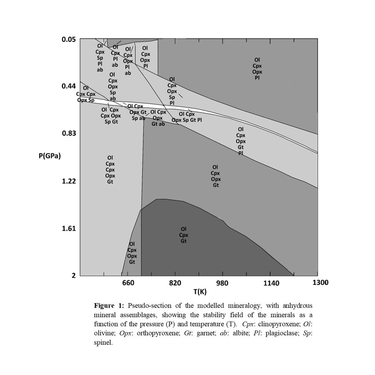
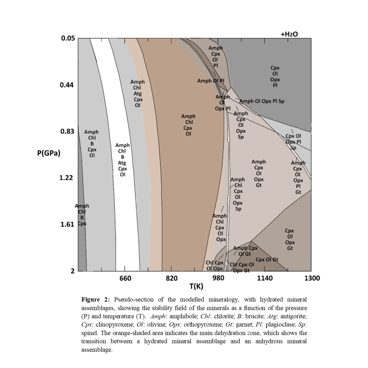
How to cite: Cioria, C. and Mitri, G.: Model of the mineralogy of the deep interior of Triton, Europlanet Science Congress 2022, Granada, Spain, 18–23 Sep 2022, EPSC2022-492, https://doi.org/10.5194/epsc2022-492, 2022.
As seen by the Hayabusa spacecraft the regolith on the surface of asteroid Itokawa shows strong segregation by particle size [1].
Approaches to explain this segregation are either focused on the bulk material, like the Brazil Nut Effect, as obeserved in agitated granular media [2, 3]. Or the explanations stems from the idea of impact driven segregation, as proposed by Sinbrot with the Ballistic Sorting Effect [4]. Both kinds of effect may even contribute concurrently [5].
We designed an experiment to investigate impact driven segregation. To experimentally recreate the surface of an asteroid [6], we utilize the microgravity of the Bremen drop tower. Inside the 10^-6 m/s² microgravity environment in the drop tower capsule, we use a linear stage to accellerate a vacuum chamber containing a granular bed (e.g. our asteroid surface) at a constant acceleration of 2*10^-4m/s². A launcher mechanism then hauls a basalt impactor onto this surface. The outcome of the impact is tracked using three cameras, enabling us to determine the coefficient of restitution (COR), defined as the ratio of the impactor's absolute velocities before and after the impact.
This ratio is a good measurement for the energy disspiation happening during the impact and therefore the relative mobility of the impactor after rebounding. The COR measured in our experiments shows an interesting behaviour, especially for finely powdered beds. While the BSE proposed by Shinbrot only requires a decline of the COR with rising bed particle size, we observe an increased COR for very fine particles as well. Using numerical simulations we find this effect to be caused by inter-partilce cohesion. In detail, we show that without cohesion no such non-monotonic behavior is possible.
From our experimental and numerical results we conclude that in a low gravity environment like asteroids cohesion is important for the size-depended COR and furthermore that its non-monotonic behavior should enhance size segregation for certain particle sizes.
[1] A. Fujiwara, J. Kawaguchi, D.K. Yeomans, M. Abe, T. Mukai, T. Okada, J. Saito, H. Yano, M.Yoshikawa, D.J. Scheeres et al., Science 312, 1330 (2006)
[2] S. Matsumura, D.C. Richardson, P. Michel, S.R. Schwartz, R.L. Ballouz, Mon. Not. R. Astron. Soc. 443, 3368 (2014)
[3] C. Maurel, R.L. Ballouz, D.C. Richardson, P. Michel, S.R. Schwartz, Mon. Not. R. Astron. Soc. 464, 2866 (2016)
[4] T. Shinbrot, T. Sabuwala, T. Siu, M.V. Lazo, P. Chakraborty, Phys. Rev. Lett. 118 (2017)
[5] E. Wright, A.C. Quillen, J. South, R.C. Nelson, P. Sanchez, J. Siu, H. Askari, M. Nakajima, S.R. Schwartz, Icarus 351 (2020)
[6] K. Joeris, L. Schönau, L. Schmidt, M. Keulen, V. Desai, P. Born, J. Kollmer, EPJ Web of Conferences 249, 13003 (2021)
How to cite: Joeris, K., Schönau, L., Keulen, M., Born, P., and Kollmer, J. E.: Slow Impacts on Rubble Pile Asteroids: The Influence of Cohesion on Restitution, Europlanet Science Congress 2022, Granada, Spain, 18–23 Sep 2022, EPSC2022-541, https://doi.org/10.5194/epsc2022-541, 2022.
The project “Deciphering compositional processes in inner airless bodies of our Solar System”, selected in the framework of the ISSI-Call for proposal 2019, set out to answer two scientific questions. First, why do chemical changes induced by space weathering in the surface regolith appear to be different on Vesta, Mercury and the Moon, and what is the role and importance of mineralogy and composition? Second, bearing in mind that olivine has been identified on the Moon and on the large asteroid Vesta, whereas it has not yet been found on Mercury: what are the implications for all of these three planetary bodies?
Vesta is the parent body of the howardite, eucrite and diogenite (HED) clan of meteorites [1]. Its surface is characterized by the presence of orthopyroxenes [2], and several geological features such as impact craters, grooves, troughs, and some tholi [3]. VIR revealed that all the Vesta spectra show the typical pyroxene bands centered at 0.9 µm and 1.9 µm [4], and allowed for determining the distribution of the HED lithologies across its surface. Like Vesta, the Moon spectra also display pyroxene spectral signatures, but suggest a composition more compatible with low-Ca pyroxenes rather than orthopyroxenes, with shallower band depths and surfaces characterized by “redder” spectral slopes (reflectance increasing with the wavelengths) [5]. Conversely, unlike Vesta and the Moon, Mercury spectra appear featureless and with a steep positive spectral slope, significantly different from the other two bodies [6].
For the spectral and geological analysis of Vesta, we processed data acquired by two instruments onboard the Dawn spacecraft: the Visible and Infrared mapping spectrometer (VIR) [7] and the Framing Camera (FC) [7]. All these datasets are publicly available on the Planetary Data System [8]. We calibrated and removed the artifacts, such as in [9] and [10], then we applied the Akimov photometric correction [11] and a log-linear phase function correction to obtain the reflectance spectra. For the Moon, we used data obtained by Chandrayaan-1/Moon Mineralogy Mapper (M3) and available at [12], then we calibrated and photometrically corrected the data following standard procedures [13, 14]. Regarding Mercury, we used the MESSENGER/Mercury Dual Imaging System (MDIS), publicly available high level products [15], and the MESSENGER/Mercury Atmospheric and Surface Composition Spectrometer instrument - Visible and InfraRed Spectrometer data [16].
To simulate space weathering effects on Vesta’s surface, we performed several irradiation experiments on HED samples at the Institut d'Astrophysique Spatiale (Orsay, France). The HED analogues are provided by the Museo di Storia Naturale dell’Università degli Studi di Firenze (Florence, Italy) and Museo di Scienze Planetarie di Prato (Prato, Italy). In particular, we have 4 HED samples, the olivine-diogenite NWA6232, and the eucrites NWA4968, NWA7234, and NWA6909 (Figs. 1 and 2). The samples are chips and powders with a grain size up to 75 µm to simulate Vesta regolith. The HEDs were put in the INGMAR vacuum chamber and bombarded with He+ atoms with a 40 keV energy, to emulate space weathering conditions.
Space weathering effects are linked to several factors, such as impacts (shock, vaporization, fragmentation, heating, melting, and ejecta formation), radiation damage, and sputtering (due to cosmic rays or solar wind), diurnal thermal cycling, and ion implantation [17, 18]. These phenomena cause the formation of nanophase iron particles (npFe0) in both the agglutinates and in the accreted rims on individual grains [17, 18], inducing spectral reddening and the reduction of band depths [18]. On the Moon, all these effects are evident in the spectra. Mercury has featureless spectra with steep, positive spectral slopes, varying with the terrain type, while on Vesta the band depth reduction is mainly due to the presence of opaque mineralogical phases, and the redder surfaces are observed in the so-called “orange material” units, corresponding to the Oppia and Octavia crater regions. The application of multivariate statistical methods to the Vesta global spectral maps, shows no evidence of diffuse olivine regions, in agreement with previous results [19, 20, 21]. A detailed analysis of Vesta, the Moon and Mercury is the key for understanding how the space weathering processes influence planetary bodies located in different regions of the Solar System, while the olivine distribution has deep implications for their origin and evolution.
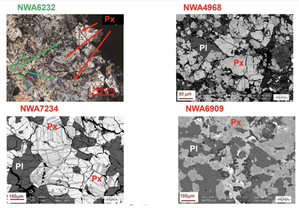
Figure 1: Close up of the HED analogues considered for our study.
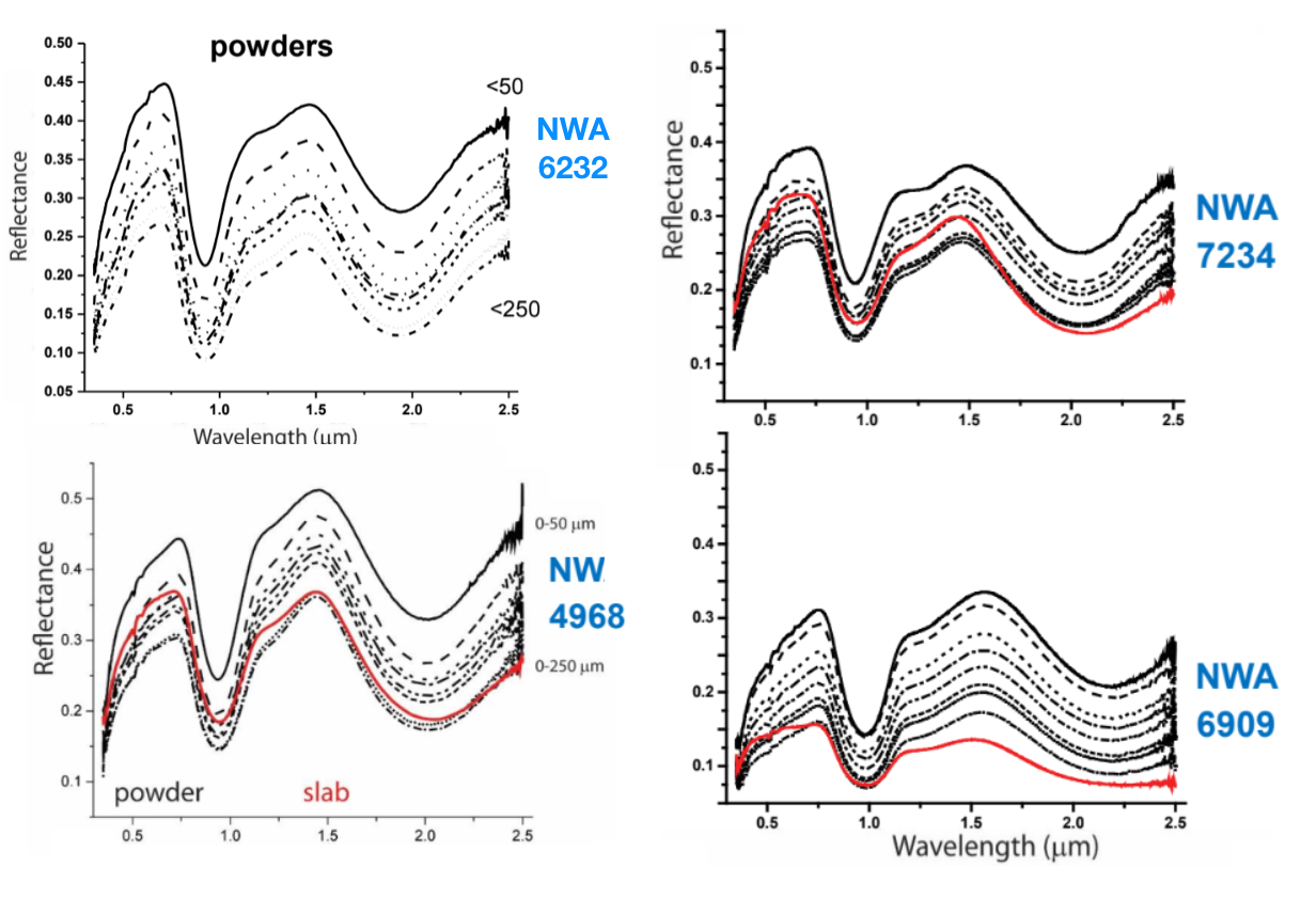
Figure 2: Reflectance spectra of the HED samples considered for this project.
Acknowledgements: This work is supported by the International Space Science Institute (ISSI) - Bern (Switzerland), project n°485, “Deciphering compositional processes in inner airless bodies of our Solar System” selected in the framework of the ISSI-call for proposal 2019.
References: [1] Feierberg, M.A., Drake, M.J., 1980, Science 209. [2] McCord, T. B., et al., 1970, Science 168. [3] Special Issue: The Geology of Vesta, Icarus 244. [4] De Sanctis et al., 2012, Science. [5] Sivakumar, V., 2017. Geoscience Frontiers 8. [6] Izenberg, N., et al., 2014, Icarus 228. [7] Sierks, M. et al., 2011, Space Sci. Rev. 163. [8] De Sanctis et al., 2011, Space Sci. Rev. 163. [9] https://pds-smallbodies.astro.umd.edu/data_sb/target_asteroids.shtml#4_Vesta. [10] Carrozzo, F. G., et al., 2016, Rev. of Sci. Instr. 87. [11] Rousseau, B. et al., 2020, Rev. of Sci. Instr. 91. [12] Schröder, S. E., et al., 2013, Planetary and Space Science 85. [13] https://ode.rsl.wustl.edu/moon/. [14] https://pds-imaging.jpl.nasa.gov/documentation/Isaacson_M3_Workshop_Final.pdf. [21] Besse, S. et al., 2013, Icarus, 222. [15] https://messenger.jhuapl.edu/Explore/Images.html#global-mosaics. [16] https://pds-geosciences.wustl.edu/missions/messenger/mascs.htm. [17] S. Noble et al., 2005, MAPS, [18] C.M. Pieters and S.K. Noble, 2016. JGR. [19] Ammannito, E., et al., 2013, Nature, [20] Ruesch, O., et al., 2014, JGR 119, [21] Palomba, E. et al., 2015, Icarus 258.
How to cite: Zambon, F., Brunetto, R., Combe, J.-P., Klima, R., Rubino, S., Stephan, K., Tosi, F., Besse, S., Barraud, O., Carli, C., Donaldson-Hanna, K., Krohn, K., Nava, J., Pratesi, G., and Rothery, D.: New updates from ISSI project n° 485, Deciphering compositional processes in inner airless bodies of our Solar System, Europlanet Science Congress 2022, Granada, Spain, 18–23 Sep 2022, EPSC2022-666, https://doi.org/10.5194/epsc2022-666, 2022.
Past, present and future small body missions include onboard accelerometers that are used either by main spacecraft during surface interactions such as sampling or touching the surface [1-2], or by lander packages deployed to the surface [3-6]. All surface interactions provide a wealth of information about the behaviour and the properties of surface materials but accelerometer data is particularly valuable. However, particular care must be taken to correctly account for the low gravity environment when interpreting the measurements. As long as the proper (Froude number) scaling is applied, the collision duration and penetration depth derived from the acceleration data can be used to infer surface properties such as the internal friction angle or the bulk density of the material [7].
Previous work has demonstrated the link between collision velocity and peak acceleration in both terrestrial and low-gravity experimental trials [8-9]. Here we will present recent experimental results investigating the link between accelerometer data and the surface properties. The collision velocity is adjusted by modifying the drop height of the projectile and impacts are performed into several different surface materials (Fig. 1).
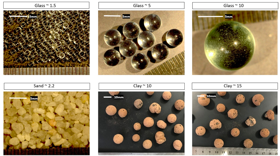
Figure 1. The granular materials used in the experimental trials
To obtain the in-situ acceleration profile during the collision, we use a projectile that contains an accelerometer. We apply the same data processing for the accelerometer measurements as used in previous work [8-9] to extract the drop height (zdrop), the collision velocity (vc), the collision duration (tstop) and the peak acceleration (apeak). In addition, we also extract the time between the instant the projectile makes contact with the ground and the moment when the projectile is at its peak acceleration (tpeak), the mean amplitude of acceleration fluctuations after the peak acceleration, and the frequency of these fluctuations (Fig. 2). As noted in previous work [10,11], the acceleration profiles have a clear dependence on particle size (Fig. 3). In this talk we will present new experimental results and discuss the information that can be extracted from accelerometers about the surface properties during .
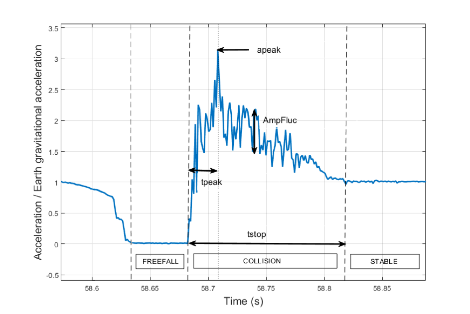
Figure 2: Typical profile measured by an in-situ accelerometer in a spherical projectile during an impact into granular material. See text for description of the variables indicated.
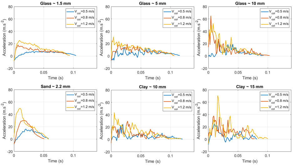
Figure 3: Acceleration profile during the impacts with different granular materials, and different collision velocities: 0.5 m/s (blue), 0.8 m/s (red), 1.2 m/s (yellow).
Acknowledgements
The authors acknowledge funding support from the European Commission's Horizon 2020 research and innovation programme under grant agreement No 870377 (NEO-MAPP project). This project also received funding from the Centre National d'Etudes Spatiales (CNES) and CS acknowledges PhD research grant funding from ISAE-SUPAERO.
References:
[1] Lauretta, D.S. and the OSIRIS-REx Team, 2021, March. The OSIRIS-REx Touch-and-Go Sample Acquisition Event and Implications for the Nature of the Returned Sample. In Lunar and Planetary Science Conference (No. 2548, p. 2097).
[2] DellaGiustina D., et al. 2022, OSIRIS-APEX: A PROPOSED OSIRIS-REX EXTENDED MISSION TO APOPHIS, Apophis T-7 Years 2022 (LPI Contrib. No. 2681)
[3] Lorenz, R.D., et al. 2009. Titan surface mechanical properties from the SSP ACC–I record of the impact deceleration of the Huygens probe.
[4] Biele, J., Ulamec, S., Maibaum, M., Roll, R., Witte, L., Jurado, E., Muñoz, P., Arnold, W., Auster, H.U., Casas, C., Faber, C., and others, 2015. The landing (s) of Philae and inferences about comet surface mechanical properties. Science, 349(6247), p.aaa9816.
[5] Michel et al., 2022, The ESA Hera mission: Detailed characterisation of the DART impact outcome and of the binary asteroid (65803) Didymos, The Planetary Science Journal (accepted)
[6] Michel, P., et al. 2022, The MMX rover: performing in situ surface investigations on Phobos. Earth Planets Space 74, 2
[7] Sunday, C., et al. 2022. The influence of gravity on granular impacts-II. A gravity-scaled collision model for slow interactions. Astronomy & Astrophysics, 658, p.A118.
[8] Murdoch, N., et al. 2017. An experimental study of low-velocity impacts into granular material in reduced gravity. Monthly Notices of the Royal Astronomical Society, 468(2), pp.1259-1272.
[9] Murdoch, N., et al. 2021. Low-velocity impacts into granular material: application to small-body landing. Monthly Notices of the Royal Astronomical Society, 503(3), pp.3460-3471.
[10] Clark et al., 2013, Granular impact dynamics: Fluctuations at short time-scales, AIP Conference Proceedings 1542, 445-448
[11] Duchêne, A., et al. 2022, A Machine Learning Approach For Estimating Asteroid Surface Properties from Accelerometer Measurements, Lunar and Planetary Science Conference 2022, no. 1563
How to cite: Murdoch, N., Duchêne, A., Segovia-Otera, J., Drilleau, M., Stott, A., and Sunday, C.: What can we learn from an in-situ accelerometer during surface interactions?, Europlanet Science Congress 2022, Granada, Spain, 18–23 Sep 2022, EPSC2022-910, https://doi.org/10.5194/epsc2022-910, 2022.
SB9 | Latest Science Results in Planetary Defence
The impact processes are ubiquitous in the solar system, as one of the fundamental mechanisms driving the evolution of asteroids and comets[1]. From small meteorite impacts to gigantic Moon-forming collisions[2], the impact cratering formation holds key insights pointing out the dynamic history of our solar system from 4.5 billion years ago. Thanks to the rapid progress in numerical modeling and computational resources, high-resolution numerical models offer a powerful framework for expanding our knowledge of the impact cratering phenomena. Meanwhile, planetary defense missions have steeply advanced in characterizing Near-Earth Objects (NEO), such as NASA's upcoming DART mission[3], which will deflect the orbit of Dimorphos through a kinetic impactor. A few years after the DART impact, the Hera mission by European Space Agency (ESA)[4] will rigorously portray the consequences of the collision, from cratering to exploring the interior and dynamics. Several numerical efforts have recently provided significant insights on impact cratering and ejecta dynamics in response to the DART impactor. Raducan et al. (2019)[5], for example, have comprehensively reported several factors that affect the Dimorphos' response, from target layering and strength[6] to the projectile obliquity[7]. In the present study, after verifying our results using the impactor/target constraints[5-7], we have further examined the consequences of DART impact, focusing more on the impact-generated porosity and gravity anomalies. To accomplish this, we performed hypervelocity impact simulations by the iSALE2D shock physics code[8-10] set up for a variety of target scenarios, ranging from low-cohesion gravity-dominated to high-cohesion stress-dominated regimes. Our simulation results shed new light on the detailed picture of cratering formation in the aftermath of the DART impact.
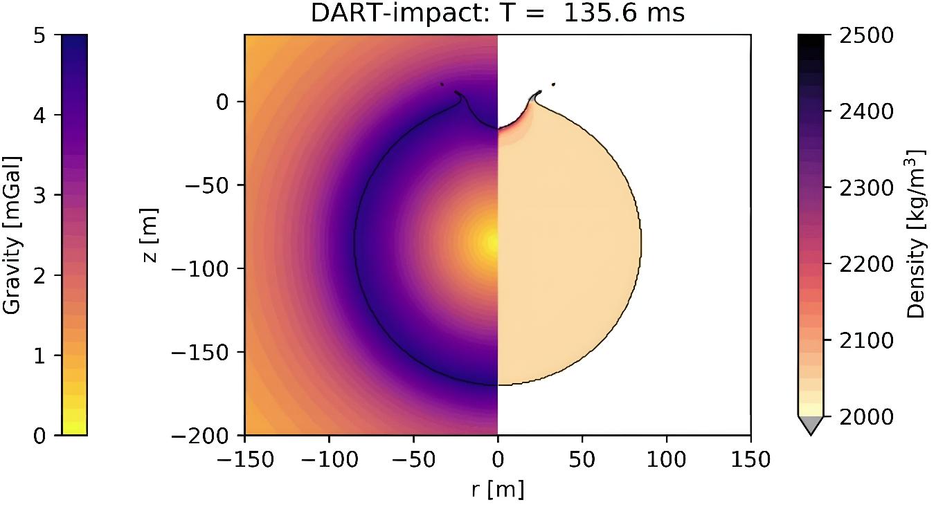
Figure 1: DART impact-generated gravity and density distribution on asteroid Dimorphos.
References
[1] Holsapple, K. A. (1993). The scaling of impact processes in planetary sciences. Annual review of earth and planetary sciences, 21(1), 333-373.
[2] Wada, K., Kokubo, E., & Makino, J. (2006). High-resolution simulations of a Moon-forming impact and postimpact evolution. The Astrophysical Journal, 638(2), 1180.
[3] Michel, P., Küppers, M., & Carnelli, I. (2018). The Hera mission: European component of the ESA-NASA AIDA mission to a binary asteroid. 42nd COSPAR Scientific Assembly, 42, B1-1.
[4] Cheng, A. F., Rivkin, A. S., Michel, P., ... & Thomas, C. (2018). AIDA DART asteroid deflection test: Planetary defense and science objectives. PSS, 157, 104-115.
[5] Raducan, S. D., Davison, T. M., Luther, R., & Collins, G. S. (2019). The role of asteroid strength, porosity and internal friction in impact momentum transfer. Icarus, 329, 282-295.
[6] Raducan, S. D., Davison, T. M., & Collins, G. S. (2020). The effects of asteroid layering on ejecta mass-velocity distribution and implications for impact momentum transfer. PSS, 180, 104756.
[7] Raducan, S. D., Davison, T. M., & Collins, G. S. (2022). Ejecta distribution and momentum transfer from oblique impacts on asteroid surfaces. Icarus, 374, 114793.
[8] Amsden, A., Ruppel, H., and Hirt, C. (1980). SALE: A simplified ALE computer program for fluid flow at all speeds. Los Alamos National Laboratories Report, LA-8095:101p. Los Alamos, New Mexico: LANL.
[9] Collins, G. S., Melosh, H. J., and Ivanov, B. A. (2004). Modeling damage and deformation in impact simulations. Meteoritics and Planetary Science, 39:217--231.
[10] Wünnemann, K., Collins, G., and Melosh, H. (2006). A strain-based porosity model for use in hydrocode simulations of impacts and implications for transient crater growth in porous targets. Icarus, 180:514--527.
How to cite: Senel, C. B. and Karatekin, O.: Hypervelocity impact simulations of DART on asteroid Dimorphos: Impact-generated porosity and gravity anomalies, Europlanet Science Congress 2022, Granada, Spain, 18–23 Sep 2022, EPSC2022-404, https://doi.org/10.5194/epsc2022-404, 2022.
Science rationale: Our knowledge of the internal structure of asteroids entirely relies on inferences from remote sensing observations of the surface combined with theoretical modeling [1]. Is Apophis a rubble-pile, as expected, or a monolithic rock, and how high is the porosity? What is the typical size of the constituent blocks? Are these blocks homogeneous or heterogeneous? If Apophis is bilobed, how does the material differ between each lobe?
After many asteroid rendezvous and fly-by missions from different nations, these crucial and yet basic questions remain open. Direct measurements of the deep interior structure and composition are needed to better understand the accretion and dynamical evolution of asteroids in general. These measurements at Apophis in particular will directly improve our ability to understand and predict stability conditions as well as to interpret the response of Apophis to the tidal forces induced by its close approach to the Earth. This information is also crucial to plan any interaction of a spacecraft with Apophis and other similar asteroids, especially for Planetary Defense purposes.
Direct observations of asteroid subsurfaces in general are also required to better model the dynamics of granular materials in low gravity, and to determine material composition and mineralogy, while space weathering and thermal cycling alter surface properties as observed by optical remote sensing.
DROID mission concept: Radar observation of Apophis from a spacecraft is the most mature technique capable of achieving these objectives, by providing a direct measurement of its interior. This is the goal of DROID – (Distributed Radar Observations of Interior Distributions), a mission concept developed in collaboration between NASA JPL and CNES [2] and discussed in more detail in the accompanying presentation [3].
The DROID mothership will release two CubeSats each carrying a low-frequency radar. The radar will be a version of JuRa (60 MHz) [4], modified to operate in a bistatic mode and using an inter-satellite link as a synchronization channel. The mothership and the two CubeSats (daughtercraft) will also have cameras for both science and navigation.
Radar observation: Each daughtercraft radar can operate in a monostatic mode, or in a bistatic mode using the two platforms to measure the signal transmitted throughout Apophis, as CONSERT did onboard Rosetta orbiter and Philae lander [1,5,6,7].
Monostatic radar. A radar at 60 MHz offers a larger penetration (up to 100 meters or more) with a limited resolution (≈5 m). It corresponds to the instrument under implementation for the Juventas Cubesat on the Hera/ESA mission [4].
Furthermore, multi-pass processing allows us to build a 3D tomographic image of the interior to identify internal structure like layers, voids and sub-aggregates, to bring out the aggregate structure and to characterize its constituent blocks in terms of size distribution and heterogeneity at different scales (from sub-metric to global). Initial dynamics modeling of the two Cubesats orbiting Apophis at 3 body radii indicates that 20% full Doppler coverage is possible in 40 days [2,8].
Shallow subsurface characterization and radar images to support the shape modeling are also possible in this configuration, but with degraded performance due to a limited resolution.
Bistatic radar. The bistatic radar will firstly measure the signal in transmission, allowing us to achieve a direct measurement of the dielectric permittivity, which is related to composition and microporosity [6]. This objective is less demanding in terms of data volume and operation compared to full bistatic coverage. Partial transmission coverage will provide slices of the body with average characterization and its special variability. With dense coverage, benefiting from a larger diversity of observation angles, the bistatic mode will allow a complete 3D tomography [8,9]. In general, multi-angular acquisition allows for a better decorrelation of the size effect and permittivity contrast in the return power.
Ground-to-space: In addition to radar observation at close proximity, there is the possibility for joint ground-to-space radar observations at the epoch of the Apophis close approach. [10]. Such measurements would make use of high-power transmitters or sensitive radio astronomy observatories on Earth [11]. Ground-to-space configurations would be used to collect echoes in unique bistatic configurations or to collect echoes during spacecraft maneuvers at close approach (e.g., required spacecraft stand-off).
Acknowledgement: The research was carried out in part at the Jet Propulsion Laboratory, California Institute of Technology, under a contract with the National Aeronautics and Space Administration (80NM0018D0004).
References:
[1] A. Herique et al. (2018) ASR 62, 2141‑2162., [2] R. Amini et al. (2022) Apophis T-7, #2012, [3] C. Raymond et al. (2022) this meeting., [4] A. Herique et al. (2022) JuRA radar, EPSC, [5] W. Kofman et al. (2015) Science 349, aab0639.,[6] Herique et al. (2016) MNRAS 462, S516‑S532., [7] A. Herique et al. (2019) A&A 630, A6., [8] M. Haynes et al. (2021) ASR 68 (9), [9] M. Haynes et al. (2021) LPSC #1295, [10] A. Herique et al. (2019) Apophis T-9 #2029, [11] M. Haynes et al (2022) Apophis T-7 #2020
How to cite: Herique, A., Adell, P., Amini, R., Davidsson, B., Haynes, M., Fesq, L., Lorda, L., Michel, P., Raymond, C., and Verdier, N.: DROID: Bistatic low-frequency radar sounding of 99942 Apophis in 2029, Europlanet Science Congress 2022, Granada, Spain, 18–23 Sep 2022, EPSC2022-474, https://doi.org/10.5194/epsc2022-474, 2022.
The ESA HERA mission approved by the last ESA council Space19+ will be launched in 2024 to deeply investigate the Didymos binary system and especially its moonlet [1]. Onboard the Juventas small platform, The Juventas Radar -JuRa- will fathom Didymoon and provide the first direct observation of an asteroid deep interior. The characterization of the asteroids’ internal structure is crucial for science, planetary defense and exploration [2].
In 2022, DART/NASA will impact the moonlet to quantify the mechanical response of the body, mainly from ground-based observation [3]. Five years later, HERA/ESA is a unique opportunity to observe in detail the bodies, the crater and the ejecta in order to better constrain mechanical models providing a global characterization of the binary system: shape, density, dynamic properties, thermal properties and composition [4]. The Hera mothercraft will carry two CubeSats, Juventas and Milani. The small spacecraft Juventas will investigate the asteroids’ internal structure. Information about the internal structure is crucial for science, planetary defense and exploration since our current knowledge relies entirely on inferences from remote sensing observations of the surface and theoretical modeling [2].
JuRa is a monostatic radar, BPSK coded at 60MHz carrier frequency and 20MHz bandwidth, inherited from CONSERT/Rosetta [5], [6] and redesigned in the frame of the AIDA/AIM phase A/B [4], [7]. The instrument design is under validation for a flight model delivery end of 2022.
JuRa maps the backscatter coefficient (sigma zero - s0) of the surface or subsurface, which quantifies the returned power per surface or volume unit. It is related to the degree of heterogeneity at the scale of the wavelength and to the dielectric contrast of heterogeneities, giving access to both, the sub-meter texture of the constituent material and larger scale structures.
- The first objective of JuRA is to characterize the moonlet’s interior, to identify internal geological structure such as layers, voids and sub-aggregates, to bring out the aggregate structure and to characterize its constituent blocks in terms of size distribution and heterogeneity at from submetric to global scale.
- The second objective is to estimate the average permittivity and to monitor its spatial variation in order to retrieve information on its composition and porosity. Radar bypasses the near surface alteration by space-weathering and thermal-cycling as observed with optical remote sensing. The observation of the structure and composition of the moonlet will provide constraints on the mechanical model of the impact process.
- The same characterization applied to the main asteroid of the binary system is among the secondary objectives, to detect differences in texture and composition. When compared to the observation of the moonlet, it will constraint the model of binary system formation to discriminate between progressive versus catastrophic process and more generally on the stability conditions of the system.
In this talk, we will review the JuRa science objectives and the instrument development status. We will show the results of the model end-to-end tests and the corresponding instrument performances. Then we will present the proposed operation strategy and the developed approaches for data processing.
Acknowledgments
- Hera is the ESA contribution to the AIDA collaboration.
- Juventas and JuRa are developed under ESA contract supported by national agencies.
- JuRa is built by Emtronix (LU), UGA/IPAG (FR), TU Dresden (DE), Astronika (PL) and FZ (CZ). Juventas is built by Gomspace (LU). Juventas navigation plan is developed by GMV (RO)
- This project has received funding from the European Union’s Horizon 2020 research and innovation program under grant agreement No 870377 (project NEO-MAPP).
References
[1] P. Michel et al., « European component of the AIDA mission to a binary asteroid: Characterization and interpretation of the impact of the DART mission », Advances in Space Research, vol. 62, no 8, p. 2261‑2272, oct. 2018, doi: 10.1016/j.asr.2017.12.020.
[2] A. Herique et al., « Direct observations of asteroid interior and regolith structure: Science measurement requirements », Advances in Space Research, vol. 62, no 8, p. 2141‑2162, oct. 2018, doi: 10.1016/j.asr.2017.10.020.
[3] A. F. Cheng et al., « Asteroid Impact & Deflection Assessment mission: Kinetic impactor », Planetary and Space Science, vol. 121, p. 27‑35, févr. 2016, doi: 10.1016/j.pss.2015.12.004.
[4] P. Michel et al., « Science case for the Asteroid Impact Mission (AIM): A component of the Asteroid Impact & Deflection Assessment (AIDA) mission », Advances in Space Research, vol. 57, no 12, p. 2529‑2547, juin 2016, doi: 10.1016/j.asr.2016.03.031.
[5] W. Kofman et al., « The Comet Nucleus Sounding Experiment by Radiowave Transmission (CONSERT): A Short Description of the Instrument and of the Commissioning Stages », Space Science Reviews, vol. 128, no 1‑4, p. 413‑432, mai 2007, doi: 10.1007/s11214-006-9034-9.
[6] W. Kofman et al., « Properties of the 67P/Churyumov-Gerasimenko interior revealed by CONSERT radar », Science, vol. 349, no 6247, p. aab0639, juill. 2015, doi: 10.1126/science.aab0639.
[7] A. Herique et al., « A radar package for asteroid subsurface investigations: Implications of implementing and integration into the MASCOT nanoscale landing platform from science requirements to baseline design », Acta Astronautica, mars 2018, doi: 10.1016/j.actaastro.2018.03.058.
How to cite: Herique, A., Plettemeier, D., and Kofman, W. and the JuRa Team: JuRa: the Juventas Radar on Hera to fathom Didymoon, Europlanet Science Congress 2022, Granada, Spain, 18–23 Sep 2022, EPSC2022-487, https://doi.org/10.5194/epsc2022-487, 2022.
Asteroids have inhabited the Solar System since its formation, and some of them may pose risks to life on Earth due to the possibility of collision with our planet. The most emblematic case of a catastrophic impact, with very significant implications for life, is the asteroid that struck the Earth 66 million years ago, forming the Chicxulub crater in the Gulf of Mexico, and causing the extinction of about 75% of all life forms on Earth. But despite this and several other events that continue to occur on smaller scales, this theme is rarely addressed by sciences, especially in Brazil. When approached by the press, it is usually under an alarmist and poorly grounded from the point of view of science.
This research aimed to analyze the level of awareness related to the importance of planetary defense among university students, as well as on ways to properly communicate the characteristics and risks related to this phenomenon to society. Besides searching for ways to defend the Earth from a possible future cosmic impact, one of the main goals of Planetary Defense is to make the population aware of its characteristics, frequency of occurrence, risks and consequences.
We focused on this subject using Science communication strategies, such as the creation of an Instagram page, where it was sought and perfected to put together posts about Planetary Defense in a simple way to reach non-specialist audiences. Thus, forms and languages have been sought to convey the facts surrounding meteoritic impacts in a way that they can be understood by the population, thus attracting the necessary attention and avoiding possible misinformation and/or panic.
We employed a semi-quantitative methodology that begins by presenting what asteroids and comets are, showing simulations of large impact events, and detailing physical phenomena arising from encounters between asteroids and the Earth. Measures to protect the planet were also analyzed and how institutions such as NASA (National Space Agency, United States) and ESA (European Space Agency, European Community) have contributed with research and equipment for planetary defense.
In addition, we combined this methodology with a semi-structured survey questionnaire. The survey was aimed at investigating society's perception of the potential risks of impacts of celestial bodies against the Earth, using students enrolled at the State University of Campinas (Unicamp, Brazil). as a sampling population.
The survey´s results refer to a total 150 responses, Fig. 1 shows that the large majority of the UNICAMP’ students don’t have previous knowledge of the concept of Planetary Defense, and that they also do not consider the topic as relevant. This shows the need for awareness dissemination regarding the risk of asteroid impacts, the only natural disaster that can be predicted in advance.
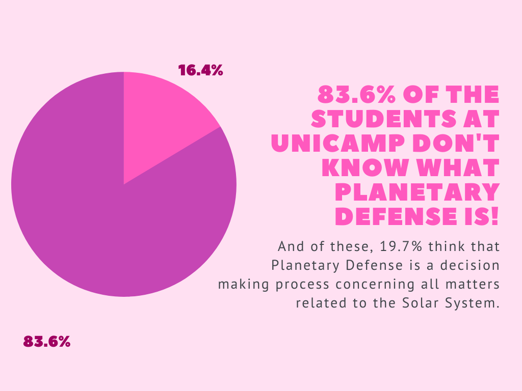
Figure 1: Survey questionnaire about society's perception of the potential risks of impacts of celestial bodies against the Earth.
As part of the study, a series of activities were developed at the University of Campinas to mark Asteroid Day 2022, celebrated annually on June 30th. During two days, a number of guest speakers presented topics related to Planetary Defense to an audience comprising Unicamp´s students and faculty members, as well as the general public, mostly high-school students and school teachers. The results contributed significantly for raising the awareness about planetary defense and for disseminating the scientific knowledge on asteroid impacts and their risk to Earth and to humankind.
Still part of Asteroid Day 2022, a series of interactive activities were developed with children at the city of Campinas Planetarium. These included workshops on rocket launching towards "asteroids", for transmitting the concept of the DART Mission to the kids and their parents. Presentations were also made on general themes about planetary sciences, as well as an astrophotography workshop held at the Campinas Municipal Observatory.
Although the study is still in progress, our preliminary conclusions are that there is very scarce knowledge of what Planetary Defense is, or recognition of its importance, even among higher education students of one of the most prestigious universities in Brazil. This shows how much Planetary Sciences are undervalued, and particularly, the theme of Planetary Defense. We expect that, by the end of this study, adequate ways will be exploited for disseminating knowledge on these topics.
How to cite: Mistro, M. E. T., Crosta, A. P., Costa, J. O. P., and Schmidt, S. C.: Planetary Defense: Public Perception and How to Communicate, Europlanet Science Congress 2022, Granada, Spain, 18–23 Sep 2022, EPSC2022-682, https://doi.org/10.5194/epsc2022-682, 2022.
The NEO Coordination Centre (NEOCC) is one of the key components of ESA’s Planetary Defence activities. Among its goals, it has a mandate to coordinate, collect and analyse telescopic observations of NEOs. To reach this objective, we developed a wide network of observational assets. In this contribution, we discuss some of the latest results obtained thanks to this unique global network.
In the recent years, ESA has strengthened its network of follow-up telescopes. It now has direct access to the Optical Ground Station (Tenerife, Spain) and the Calar Alto Schmidt telescope (fully dedicated to NEOCC activities - Spain). Via dedicated contracts, it also has allocated time in the LCO network, as well as telescopes in Australia (Zadko), Namibia (6ROADS), Reunion and India. Scientific collaboration & agreements granted time with ESO’s VLT and Korean’s BOAO and SOAO facilities.
Regarding future observational means, ESA is currently continuing the construction of the Flyeye telescope. This is a 1-meter class telescope with an ultra-wide field of 7º by 7º that will be installed on top of Monte Mufara (Italy). The Flyeye will be a remote-controlled telescope, while data will be automatically analysed by a dedicated pipeline, with the overall objective of reducing to a minimum the human intervention.
The mentioned observational assets available to our observers are used for a variety of observations. The main goal is of course the acquisition of follow-up observations, both on short notice and at the faint end of an object's observability window. We employ our smaller but geographically-distributed telescopes to quickly react to discoveries of possible new high-priority objects, such as imminent impactors. Larger assets, such as VLT, are instead routinely scheduled to obtain astrometry of risk list objects, down to magnitude ~27. With some specific telescopes we are also focusing on twilight and low-elongation observations, which are essential to track and characterize specific classes of objects, such as Atiras or Earth Trojans.
In addition to these regular observations, we also use some of the telescopes to attempt challenging or innovative observation techniques. For example, we are experimenting with the possibility to use modest sub-meter-size telescopes to obtain detections of important objects down to magnitude ~24, by observing the same target for an entire night and then stacking hundreds of frames on the motion of the object. These capabilities are made possible by recent advancements in GPU processing, which are also opening the way to new image analysis modes, such as synthetic tracking. We are also pioneering the so called "negative recovery" technique, using targeted non-detections of risk list objects to exclude their impact solutions, even without recovering the object itself.
Finally, we are active players in international campaigns dedicated to specific NEOs or observational challenges. This includes both our participation in internationally-led efforts, such as those managed by IAWN, and the organization of our own campaigns, such as a recent one dedicated to the astrometric coverage of the Earth fly-by of BepiColombo as a proxy to test the observational capabilities of our network on very close approachers.
All those observations are supplemented by the operations of our own orbit determination and impact monitoring software system (so-called AstOD) that allows constraining with the best possible accuracy the orbits of the observed objects and the possible impact chances with the Earth in the next 100 years. In what regards the threat monitoring over imminent impactors, we count on the Meerkat tool, which bases its automated operation on the use of systematic ranging and allows detecting and warning our staff of those cases, as recently occurred with 2022 EB5.
How to cite: Cano, J. L., Micheli, M., Conversi, L., Fohring, D., Moissl, R., Koschny, D., Faggioli, L., Gianotto, F., Kresken, R., Ramirez Moreta, P., Oliviero, D., Petrescu, E., Rudawska, R., and Frühauf, M.: Recent observational highlights from ESA’s Planetary Defence Office, Europlanet Science Congress 2022, Granada, Spain, 18–23 Sep 2022, EPSC2022-1084, https://doi.org/10.5194/epsc2022-1084, 2022.
Understanding of shallow angle impacts (termed "oblique") comes from planetary bodies other than Earth, and also comes from modelling published by various workers over the past two decades or so. Another comparator source is the Southern Mt Lofty Ranges and Kangaroo Island impact in South Australia, which has not been dated other than being >35 mya. At previous conference attendances the case has been built that the oblique impact in SA was from the south rather than in the plane of the ecliptic, which raises the new question how common is such an event in the solar system. A digital elevation model from the Mars Orbiter Laser Altimeter has here been used to assess the occurrences of oblique impacts on Mars, focussing on the northern hemisphere. A large impact crater at 7 degrees N / 178 degrees E on Mars matches the criteria and additionally has the same impact approach direction as the Southern Mt Lofty Ranges craters, implying that the orbital plane of that impactor may have been similar or the same as that of the latter. The large scale of the particular crater identified on Mars forces a reassessment of the sizes of additional candidate Australia craters beyond the Southern Mt Lofty Ranges and Kangaroo Island impact sites. A digital elevation model of a central band of Australia, some 600 km wide, is analysed for candidate sites, while indicators of meteorite disintegration during oblique impacts are used to inform the study and to shortlist candidate sites.
How to cite: Moore, R.: Linking a large oblique-impact crater on Mars to the Southern Mt Lofty Ranges multiple impact event in South Australia – inference for latter event size and scope, Europlanet Science Congress 2022, Granada, Spain, 18–23 Sep 2022, EPSC2022-1201, https://doi.org/10.5194/epsc2022-1201, 2022.
SB10 | Observing and modelling meteors in planetary atmospheres
Abstract
In this paper we present the results obtained from the spectral analysis using the wavelet technique of a time series of brightest fireballs to look for periodicities associated with other bodies of our Solar System. The spectra show four periodicities at 106.2 days, 12.7 days, 2.5 days, 10.3 years and 4.6 years. In particular the periodicities around 12.7 and 2.5 days could be related to the Carrington rotation period.
Introduction
One of the main problems of Planetary Sciences is to understand the dynamical behavior of asteroids, meteors and meteoroids inhabiting near our planet, mainly those that fall on terrestrial surface. These bodies feel the planetary and solar gravitational influence when they travel across the interplanetary medium or mainly when they are in the terrestrial neighborhood of one of those bodies. The detection of meteoroids falling on Earth using several instruments has been important because it has permitted to obtain very useful data. The analysis of these data can help to identify the physical interactions that occur between these bodies and the rest of the bodies in the solar system. Additionally in recent decades, multiple modeling and numerical simulation works have been carried out to fully understand the origin of such interactions.
The spectral method
A time series of brightest fireballs from January, 1998 to December, 2020 was spectrally studied using the wavelet technique to look for periodicities related with Solar System bodies relationships. The data were taken from the Near Earth Object Program (https://cneos.jpl.nasa.gov/fireballs). Because of this time series has gaps, the wavelet transform was used to do the spectral analysis. The method was applied using the Morlet function (eq. 1) [1] to analyze the power spectral density (PSD) of brightest fireball meteors [1], [2], [3].
![]() (1)
(1)
Where ω0 and η are both non-dimensional frequency and time parameter respectively
Results and discussion
Five periodicities were identified from the wavelet spectral analysis (figure 1). They are located at 2.5 days, 12.7 days, 106.2 days, 4.6 years and 10.3 years. The figure 1 shows the power spectral density spectra (PSD) where these periodicities can be seen on the right side of the plot. They are inside the cone of influence (COI) and were obtained with a confidence level of 85%. The uncertainties of every peak position were obtained from the peak full width at half maximum.
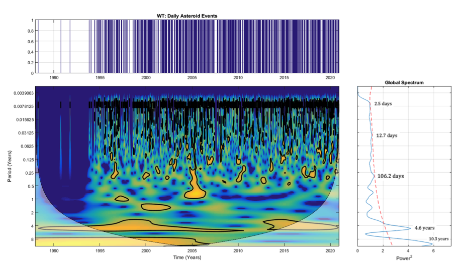
Figure 1: PSD of a time series of brightest fireballs from January, 1998 to December, 2020. On the right side of the plot, five peaks at 2.5, 12.7 and 106.2 days and at 4.6 and 10.3 years are shown.
In particular the periodicity around 12.7 days could be the first harmonic of the Carrington rotation period (27 days), [4] indicating that the solar gravitational force could be modulating the meteoroids entrance on the Terrestrial atmosphere. Carrington rotation has been detected in several time series as is the case of solar spots, storm sudden commencements, cosmic rays, among others. The periodicity around 2.5 days, it could be a small harmonic of the solar rotation period.
The mechanism behind the relationship between the variable solar radiation (due to its rotation and the solar cycle) and the fall of small asteroids to Earth´s atmosphere could be associated to the Yarkovsky and /or YORP effects. Several works have shown that the solar radiation is able to modify asteroidal orbits and rotational periods [5, 6], and it is possible that the periodicity in the variability of this radiation be the cause of periodicities in the falling of asteroidal material observed in this work. Respect to the periodicities around 4.6 and 10.3 years, they could be related to the magnetic solar cycle. The 4.6 years periodicity could be related to Jupiter too. According to NASA (https://solarsystem.nasa.gov/planets/jupiter/overvie w/), the Jupiter orbital period is 4333 Earth days, so the ratio between this period and 1679 Earth days (̴ 4.6 year period) is almost 13/5.
Summary and Conclusions
1. The Sun could be a gravitational trigger of meteoroids from their neighborhood to Earth.
2. The periodicity around 12.7 days is possible associated with the Carrington rotation as well as the 2.5 days periodicity.
References
[1] Torrence, Ch., Compo, G. P.: A practical guide to wavelet analysis, Bulletin of American Meteorogical Society, vol. 79, No. 1, pp. 61-78, 1998. https://doi.org/10.1175/1520-0477(1998)079<0061:APGTWA>2.0.CO;2
[2] Soon, W., Dutta, K., Legates, D. R., Velasco, V., Zhang, W.: Variation in surface air temperature of China during the 20th century, J. Atmos. Sol-Terr. Phy. 73, pp. 2331-2344, 2011.
[3] Velasco Herrera, V. M., Soon, W., Velasco Herrera, G., Traversi, R., Horiuchi, K.: Generalization of the cross-wavelet function, New Astronomy, 56, pp. 86-93, 2017.
[4] Nayar, S. R. P.: Periodicites in solar activity and their signature in the terrestrial environment, ILWS Workshop 2006, Goa, India, February 19-24, pp. 1-9, 2006.
[5] Farnocchia, D., Chesley, S. R., Takahashi, Y., Rozitis, B., Vokrouhlický, D., Rush, B. P., Mastrodemos, N., Kennedy, B.M., Park, R. S., Bellerose, J., Lubey, D. P., Velez, D., Davis, A.B., Emery, J. P., Leonard, J. M., Geeraert, J., Antreasian, P.G., Lauretta, S.: Ephemeris and Hazard Assessment for Near-Earth Asteroid (101955) Bennu Based on OSIRIS-REx Data, Icarus, 369, https://doi.org/10.1016/j.icarus.2021.114594, 2021.
[6] Zegmott, T. J., Lowry, S. C., Rozek, A., Rozitis, B., Nolan, M. C., Howell, E.S., Green, S. F., Snodgrass, C., Fitzsimmons, A., Weissman, P. R.: Detection of the YORP Effect on the Contact Binary (68346) 2001 KZ66 from Combined Radar and Optical Observations, Monthly Notices of the Royal Astronomical Society. 507, pp. 4914-4932, https://doi.org/10.1093/mnras/stab2476, 2021.
How to cite: Maravilla, D., Pazos, M., and Cordero, G.: Are fireballs fall on Earth modulated by our star?, Europlanet Science Congress 2022, Granada, Spain, 18–23 Sep 2022, EPSC2022-26, https://doi.org/10.5194/epsc2022-26, 2022.
1. Introduction
The Fireball Recovery and Inter Planetary Observation Network (FRIPON) network [1] uses all-sky cameras in order to detect fireballs. The FRIPON network comprises over 150 cameras installed all over Europe [1]. In this work we focus on the results obtained by the Meteorite Orbits Reconstruction by Optical Imaging (MOROI) [2] component of the FRIPON network in Romania. As of May 2022, the MOROI network detects the events with the use of 13 all-sky cameras.
2. Methods
The method for computing the fireball trajectory used by FRIPON is presented in [3].
The height, velocity and slope γ of the meteoroid are the input data for computing the ballistic coefficient α and the mass-loss parameter β. We select the candidates that are likely to produce meteorites of the ground using the α-β algorithm presented in [4], [5], [6], [7].
3. Results
Starting from January 2021 (the starting moment of data fusion of the MOROI network into the FRIPON network) until the present time (May 2022) over 100 meteors were detected. We present the most spectacular events that are likely to result on a meteorite production on the surface of the Earth.

Figure 1: The outcome of the FRIPON (MOROI) detections in Romania
In Figure 1 are represented the coordinates of the meteoroids with noticeable deceleration in the (ln(αsinγ),lnβ) coordinates system. The values of the shape parameter correspond to the cases when the meteoroid doesn’t rotate (µ=0) or rotates uniformly (µ=2/3).
The boundaries (‘likely fall’, ‘possible fall’, ‘unlikely fall’) are represented for meteoroids with final mass of 50 g.
We processed the 100 detections of the FRIPON (MOROI) network in Romania. From this amount of data, we found 15 fireball events with noticeable deceleration. We found one event in the ‘likely fall’ area and three events in the ‘possible fall’ area. The fireball that is likely to produce meteorites was detected by the MOROI network on 24.11.2021 at 19:20:57 UT.
We model the dark flight trajectory of the meteoroids with the ‘likely fall’ and ‘possible fall’ outcomes and determine their strewn field with the model presented in [8], [9]. We use the wind model from the European Centre for Medium-Range Weather Forecasts (ECMWF).
A meteorite recovery campaign will be organised to identify the strewn field area.
Acknowledgement.
The work of IB and MB was partially supported by a grant of the Romanian Ministry of Education and Research, CNCS-UEFISCDI, project number PN-III-P1-1.1-PD-2019-0784, within PNCDI III. The work of IB, MB, AN was partially supported by a grant of the Ministry of National Education and Scientific Research, PNIII-P2-1214/25.10.2021, program no. 36SOL/2021. JM and MG acknowledge the Academy of Finland project no. 325806 (PlanetS).
References:
[1] Colas F., Zanda B., Bouley S., Jeanne S., Malgoyre A., Birlan M., Blanpain C., Gattacceca J., Jorda L., Lecubin J., et al. (385 more) FRIPON: a worldwide network to track incoming meteoroids. Astronomy &. Astrophys. 644, A53. doi:10.1051/0004-6361/202038649. 2020.
[2] Nedelcu D.A., Birlan M., Turcu V., Boaca I., Badescu O., Gornea A., Sonka A.B., Blagoi O., Danescu C., Paraschiv P. Meteorites Orbits Reconstruction by Optical Imaging (MOROI) Network. Romanian Astronomical Journal 28(1), 57 – 65. 2018.
[3] Jeanne, S., Colas, F., Zanda, B., Birlan, M., Vaubaillon, J., Bouley, S., Vernazza, P., Jorda, L., Gattacceca, J., Rault, J. L., Carbognani, A., Gardiol, D., Lamy, H., Baratoux, D., Blanpain, C., Malgoyre, A., Lecubin, J., Marmo, C., Hewins, P. Calibration of fish-eye lens and error estimation on fireball trajectories: application to the FRIPON network. Astronomy and Astrophysics, 627:A78. 2019.
[4] Gritsevich, M. I. The Pribram, Lost City, Innisfree, and Neuschwanstein falls: An analysis of the atmospheric trajectories. Solar System Research.42, 372–390. 2008.
[5] Gritsevich, M.I., Stulov, V.P., Turchak, L.I. Consequences of collisions of natural cosmic bodies with the Earth's atmosphere and surface. Cosmic Research vol.50, no.1, 56-64. 2012.
[6] Sansom, E.K., Gritsevich, M., Devillepoix, H.A.R., Jansen-Sturgeon, T., Shober, P.,
Bland, P.A., Towner, M.C., Cupák, M., Howie, R.M., Hartig, B.A.D. Determining Fireball Fates Using the α-β Criterion. Astrophysical Journal 885(2):115. 2019.
[7] Boaca I., Gritsevich M., Birlan M., Nedelcu, A., Boaca, T., Colas, F., Malgoyre, A.,
Zanda, B., Vernazza P., to be submitted. 2022.
[8] Moilanen, J., Gritsevich, M., Lyytinen, E., Determination of strewn fields for meteorite falls, Monthly Notices of the Royal Astronomical Society 503, 3337–3350. 2021.
[9] Boaca I., Nedelcu A., Birlan M., Boaca T., Anghel S. Mathematical model for the dark-flight trajectory of a meteoroid, Romanian Astronomical Journal, Vol. 31, No. 2. 2021.
How to cite: Boaca, I. L., Moilanen, J., Gritsevich, M., Birlan, M., Nedelcu, A., Boaca, T., Colas, F., Malgoyre, A., Zanda, B., and Vernazza, P.: Analysis of the meteorite-producing fireballs registered by the MOROI component of the FRIPON network, Europlanet Science Congress 2022, Granada, Spain, 18–23 Sep 2022, EPSC2022-160, https://doi.org/10.5194/epsc2022-160, 2022.
Several meteor clusters were observed by the video cameras deployed within the Czech Republic in recent years. Moreover, we also obtained data on another cluster which was detected above the Southern America.
In this talk the basic data on the selected meteor clusters, their atmospheric trajectories, and 3D distribution of the fragments will be provided. For example, a cluster consisting from a fireball and four fainter meteors was observed on August 23, 2020. It was a relatively compact cluster with smaller meteoroids up to 30 kilometres from the main body. Possible origin of the clusters will be discussed, too.
How to cite: Koten, P. and Čapek, D.: Meteor clusters observed by the video technique, Europlanet Science Congress 2022, Granada, Spain, 18–23 Sep 2022, EPSC2022-420, https://doi.org/10.5194/epsc2022-420, 2022.
EXOA1 | Formation, evolution, and stability of extrasolar systems
Abstract
High-precision measurements of isotopes in meteorites suggest that the early population of small bodies in the Solar System has been separated into two reservoirs by the forming Jupiter, acting as a radial barrier for these 'planetesimals' [1]. In a proposed Jupiter formation scenario [2], the solid core must grow within 1 Myr to around 20 Earth masses, then stagnate its growth for 2-3 Myr and thus separating the planetesimal reservoirs, and finally grow to the final Jupiter mass stirring and mixing the inner and outer planetesimals. The fast and early core growth is efficiently facilitated by the accretion of small 'pebble-like' objects. In order to delay the otherwise inevitable rapid runaway gas accretion for an extended period of time after the pebble accretion stops, Jupiter is proposed to be heated by slower planetesimal accretion before finally becoming massive enough to accrete a large amount of gas, reaching its present day mass.
Motivated by this proposed formation scenario of Jupiter, we investigate the consequences of a combined pebble and planetesimal accretion model for the formation of giant planets and planet formation in general [3]. We modify the Bern model of planetary population synthesis [4] with a simple model of pebble formation and accretion [5]. In a single-planet population synthesis approach, we run the model on a thousand different initial protoplanetary disks in order to probe the effects of the two solid accretion mechanisms on a population level. To uncover the interplay of the two models, we vary the amount of pebbles with respect to planetesimals.
As shown in figure 1, it proves to be difficult to form giant planets from the accretion of pebbles and planetesimals whereas both mechanisms individually are able to form giants in suitable disks. We identify the remaining accretion of planetesimals after the stop of pebble accretion to be crucial for the formation pathway of a growing planet. The envelope heating due to the accretion of solids is shown to play a critical role for the accretion of gas. A combination of enhanced inward orbital migration and delayed runaway gas accretion strongly suppresses the formation of giants in disks containing both pebbles and planetesimals.

Figure 1: Planet mass over semi-major axis snapshot after 2 Gyr of evolution for populations of one thousand disks, containing one planet. The four, otherwise identical, populations start with either only planetesimals (left), 30% pebbles (middle left), 70% pebbles (middle right), or only pebbles (right).
References
[1] Kruijer T. S., Burkhardt C., Budde G., Kleine T., 2017, Proc. Natl. Acad. Sci., 114, 6712
[2] Alibert Y., Venturini J., Helled R., et al., 2018, Nature Astronomy, 2, 873
[3] Kessler A., et al., in prep.
[4] Emsenhuber A., Mordasini C., Burn R., et al., 2021, A&A, 656, A 69
[5] Bitsch B., Lambrechts M., Johansen A., 2015b, A&A, 582, A 112
How to cite: Kessler, A., Alibert, Y., Mordasini, C., Emsenhuber, A., and Burn, R.: Giant Formation with Pebbles and Planetesimals, Europlanet Science Congress 2022, Granada, Spain, 18–23 Sep 2022, EPSC2022-114, https://doi.org/10.5194/epsc2022-114, 2022.
The size distribution of solids in the protoplanetary disk is still ill constrained [1] but is a vital parameter that influences planetary growth [2]. The typical size and spatial distribution of solids evolves throughout the planet formation process via collisions and radial drift. As the planets grow, they excite the mutual random velocities among planetesimals making their mutual collisions destructive which leads to fragmentation, reducing their typical size. This effect of self-interacting planetesimals has been found to inhibit or favor the formation of planets due to competing effects of easier accretion of smaller fragments and depletion by gas-drag induced drift [3-4]. However, previous studies have either focused on single planets and systems or have neglected concurrent effects like migration.
Therefore, we run planet formation simulations with the generation III Bern model [5] with a Eulerian 1D solid disks. The model tracks the growth and evolution of several planetary embryos from oligarchic growth to the final planetary system. We added to it a fragmentation toy model [6] to see the impact fragmentation has on planet formation. To see its influence on the diverse types of exoplanets we make use of a population synthesis approach to investigate larger parts of the parameter space [7]. This allows us to have a more complete picture of what influence the collisional evolution of planetesimals has on planet formation and to study the effects that arise from its interplay with the formation of multiple planets in the same system.
In figure 1, we show two exemple synthetic planet populations of 1000 systems with (right) and without (left) the added fragmentation model. We find multiple interesting features in our synthetic populations that arise from the fragmentation of planetesimals. The fragmentation lends more importance to specific locations in the disk where growth is enhanced like the ice line and the inner disk. In addition, it enhances the formation of giants.
In conclusion, there are significant differences in synthetic populations when including or neglecting fragmentation. This suggests that the addition of fragmentation to global planet formation models is important as a self-consistent solid disk description is vital to understand planet formation.
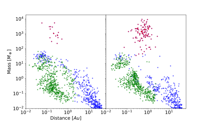
In figure 1. Comparison of a synthetic exoplanet population without (left) the added fragmentation model and one with (right). The semi major axis (in AU – log scale) is plotted on the x-axis and the planetary mass (in Earth masses – log scale) on the y-axis. Both populations are shown at an age of 5 Gyr. The Red points refer to planets with more envelope than core mass, the blue ones are icy planets (ice mass fraction larger than 1%) and the green points are rocky planets (ice mass fraction smaller than 1%).
References:
[1] Helled, R. & Morbidelli, A. 2021, in ExoFrontiers (IOP Publishing)
[2] Fortier, A., Alibert, Y., Carron, F., Benz, W., & Dittkrist, K.-M. 2012, A&A, 549, A44
[3] Guilera, O. M., de Elía, G. C., Brunini, A., & Santamaría, P. J. 2014, A&A, 565, A96
[4] Chambers, J. 2008, Icarus, 198, 256
[5] Emsenhuber, A., Mordasini, C., Burn, R., et al. 2021, A&A, 656, A69
[6] Ormel, C. W. & Kobayashi, H. 2012, The Astrophysical Journal, 747, 115
[7] Emsenhuber, A., Mordasini, C., Burn, R., et al. 2021b, A&A, 656, A70
How to cite: Kaufmann, N. and Alibert, Y.: A population level study on the influence of planetesimal fragmentation on planet formation, Europlanet Science Congress 2022, Granada, Spain, 18–23 Sep 2022, EPSC2022-135, https://doi.org/10.5194/epsc2022-135, 2022.
Although most stars exist in binary and multi systems, very few circumbinary planets (CBP) have been identified and studied. Observational biases contribute significantly to this paucity, as the orbital regions close to binaries are often unstable due to overlapping secular resonances. As we continue to improve our data reduction and analysis techniques, we can start to detect more planets farther from their stars and will therefore detect more CBPs. Through thousands of N-body simulations, we constrain the stability regions of an injected terrestrial planet around low-mass binaries, integrating the systems for 1Gyr or until instability. We then explore the potential detection and habitability of such planets. Through the 1Gyr evolution of the system, we trace the top-of-atmosphere temperature of the simulated planets to constrain the fraction that could host liquid water on their surfaces. Then, using a simple energy-balance model, we study the evolution of the planets' surface temperatures to identify which could host regions of continuous surface water.
How to cite: MacDonald, M. and Pedowitz, M.: Constraining the stability and habitability of circumbinary planets, Europlanet Science Congress 2022, Granada, Spain, 18–23 Sep 2022, EPSC2022-164, https://doi.org/10.5194/epsc2022-164, 2022.
The sailboat region was first identified by Giuliatti Winter, et al. (2010) exploring the Pluto-
Charon binary system, they identifed this unexpected stable region of S-type orbits around the dwarf
planet Pluto located at a = (0.5d, 0.7d) and e = (0.2, 0.9), where a and e are the initial values
of semi-major axis and eccentricity of particles, respectively and d is the separation of the binary.
The sailboat is associated with a family ”BD” of periodic orbits derived from the planar, circular,
restricted three-body problem. In this work, we analyzed through numerical simulations the structure
and stability of sailboat in hypothetical systems with different values of mass ratio and for several
orbital configurations.
To constrain the orbital parameters for sailboat regions, we numerically simulated several elliptic
three-body problem, exploring a large range of initial conditions. We adopt dimensionless systems
and the configuration for each simulation include a test particle in S-type orbit around the primary
body and gravitational disturbed by the secondary massive body. We set the central body as a point
of mass and a secondary with a mass equivalent to the mass ratio of the binary system (µ), with its
radius (r s ) defined as 10% of their Hill radius.
We created hypothetical systems with different mass ratio in the interval µ = [0.01, 0.30] in steps
∆µ = 0.01. The test particles were randomly distributed with semimajor axis in a = [0.45, 0.7],
considering 1 the distance between the two main bodies, the eccentricities varied from 0 to 0.99, and
initially the argument of the pericentre and inclination was set as 0º. We numerically integrated using
the REBOUND package and IAS15 integrator (Rein & Spiegel 2014) for 10 4 orbital periods of the
binary.
We analyzed the behaviour of the sailboat according to the eccentricity e of the secondary body,
looking for the maximum value for which the particles remain stable. A final set of simulations was
performed for different values of inclinations and argument of pericenter in order to determine the
extreme values for the stability.
Our results show the sailboat is robust and it exists for µ = [0.01,0.27] and for large intervals
of the argument of pericentre and inclination. This region of stability reaches its maximum size
with an argument of pericenter at 0 ◦ and 180 ◦ . The sailboat region also is present for values of
inclination > 60º and existing even retrogrades orbits in the systems with µ > 0.08.
The numerical results also showed that little changes in the eccentricity of the secondary body is
sufficient to vanish the sailboat region, for binaries system with µ > 0.12, the sailboat exists just for
values of e < 0.05.
How to cite: Pinheiro, T., Sfair, R., and Vieira, E.: Study of the Sailboat stable region for binary systens., Europlanet Science Congress 2022, Granada, Spain, 18–23 Sep 2022, EPSC2022-759, https://doi.org/10.5194/epsc2022-759, 2022.
Circumplanetary disks are regarded as birthplaces of large moons. While Jupiter has four large satellites known as Galilean moons, Titan is the only large moon around Saturn. N-body simulations using a simple power-low disk suggest a system tend to have multiple moons or loses all the moons due to inward migration. Thus, forming a single satellite system in a disk is known to be difficult.
The orbits of moons are continuously affected by the interaction with the disk, and the direction and speed of the migration depend on the disk structures, i.e., surface density and temperature. Therefore, the final configuration of the moon system is determined during the dissipation of the disk. We studied the orbital evolution of moons in various circumplanetary disks to find a way of configuring a single-large-moon system.
We model dissipating circumplanetary disks with taking the effect of opacity into account when we calculate the temperature structure. Because of this, our disk has multiple slopes, and thus, the migration speed of a moon varies with the orbital location. Then, we calculate the orbital evolution of Titan-mass moons in the final evolution stage of the disks. We performed N-body simulations with initially many satellites to see whether single-moon systems can form at the end.
We found that the radial slope of the temperature structure characterized by the dust/ice opacity produces a patch of orbits where the Titan-mass moons resist inward migration with a certain range of the viscosity. We call such a patch as “safety zone.” The safety zone assists moons initially located in the outer orbits to remain in the disk, while those in the inner orbits migrate toward the planet. When the satellite formation is not very efficient in the outer radii of circumplanetary disks, the system can end up with a single large moon at a distant from the planet while the inner orbits are cleared out. Smaller moons may stay in the inner orbits as their migration speed is slower compared to the Titan-mass ones. We demonstrated the formation of systems with single large moon around gas giants for the first time.
How to cite: Fujii, Y. and Ogihara, M.: Formation of a single large moon around a gas giant: Saturn-Titan system, Europlanet Science Congress 2022, Granada, Spain, 18–23 Sep 2022, EPSC2022-806, https://doi.org/10.5194/epsc2022-806, 2022.
The protoplanetary disk (PPD) is a complex structure. It is the birth place of protoplanetary systems. The interaction of growing planets and its surrounding PPD is also complex and not fully understand by now. The many different physical processes going on in the PPD over its life time, like accretion, outbursts, planet formation, etc. impact its evolution and structure. The evolution of such a PPD with a growing planet, implemented as a sink term, is simulated by the TAPIR code. It is an 1+1D implicit code. Due to the fact that TAPIR is an implicit code the time steps are not restricted by the CFL-conditions, therefore it is able to simulate over the whole lifetime of a PPD and examine the evolutionary behaviour of the protoplanetary disk and the influence of a forming protoplanet on it. The results show the gap formation due to mass accretion onto the planet and impact of this sink term on the total disk mass, disk lifetime and accretion rat onto the star. Also the impact of accretion bursts on the accretion rate of the planet is discussed. If the planet is placed in the dead zone the presence of outbursts leads to a quite faster planet growth since the bursts rearranges the disk structure.
How to cite: Ringseis, I.: Impact of growing planets on the evolution of protoplanetary disks, Europlanet Science Congress 2022, Granada, Spain, 18–23 Sep 2022, EPSC2022-1104, https://doi.org/10.5194/epsc2022-1104, 2022.
In close exoplanetary systems, tidal interactions are known to shape the orbital architecture of the system, modify star and planet spins, and have an impact on the internal structure of the bodies through tidal heating. Most stars around which planets have been discovered are low-mass stars and thus feature a magnetised convective envelope, as is also expected in giant gaseous planets like Hot-Jupiter. Tidal flows, and more specifically inertial waves (restored by the Coriolis acceleration, and recently discovered in the Sun) tidally-excited, are the main direct manifestation of tidal interactions in the convective envelopes of these bodies. Furthermore, inertial waves are small-scale waves that are sensitive to nonlinearities, especially in close Hot-Jupiter systems with strong tidal forcing. The nonlinear self-interaction of inertial waves is known to trigger differential rotation in convective shells, as shown in numerical and experimental hydrodynamical studies. Since inertial waves are a key contribution to the tidal dissipation in close star-planet systems, it is essential to have the finest understanding of tidal inertial wave propagation and dissipation in such a complex nonlinear, magnetised, and differentially rotating environment.
In this context, we investigate how nonlinearities affect the tidal flow properties, thanks to new 3D hydrodynamic and magneto-hydrodynamic nonlinear simulations of tides, in an adiabatic and incompressible convective shell. First, we show to what extent the emergence of differential rotation is modifying the tidal dissipation rates, prior to linear predictions. In this newly generated zonal flows, nonlinear self-interactions of tidal inertial waves can also trigger different kind of instabilities and resonances between the waves and the background sheared flow, when the tidal forcing is strong enough or the viscosity low enough. These different processes disrupt the energetic exchanges between tidal waves and the background flow, and also further modifies the tidal dissipation rates. Secondly, we present the first non-linear numerical analysis of tidal flows in a magnetised convective shell. One main effect of the magnetic field in our model is to mitigate zonal flows triggered by the nonlinear interaction of inertial waves. The consequences for tidal flows are important, since the installation of zonal flows in nonlinear hydrodynamical simulations is the main cause of significant changes in tidal dissipation and angular momentum exchanges, compared to linear predictions for a uniformly rotating body.
How to cite: Astoul, A. and Barker, A.: Nonlinear tidal interactions in the convective envelopes of low-mass stars and giant gaseous planets, Europlanet Science Congress 2022, Granada, Spain, 18–23 Sep 2022, EPSC2022-1198, https://doi.org/10.5194/epsc2022-1198, 2022.
EXOA2 | The hidden newly born planets
New ALMA observations of protoplanetary disks allow us to probe planet formation in other planetary systems, giving us new constraints on planet formation processes. Meanwhile, studies of our own Solar System rely on constraints derived in a completely different way. However, it is still unclear what features the Solar System protoplanetary disk could have produced during its gas phase. By running 2D isothermal hydro-simulations used as inputs for a dust evolution model, we derive synthetic images at millimeter wavelengths using the radiative transfer code RADMC3D. We find that the embedded multiple giant planets strongly perturb the radial gas velocities of the disk. These velocity perturbations create traffic jams in the dust, producing over-densities different from the ones created by pressure traps and located away from the planets’ positions in the disk. By deriving the images at λ = 1.3 mm from these dust distributions, we show that very high resolution observations are needed to distinguish the most important features expected in the inner part (<15 AU) of the disk. The traffic jams, observable with a high resolution, further blur the link between the number of gaps and rings in disks and the number of embedded planets. We additionally show that a system capable of producing eccentric planets by scattering events that match the eccentricity distributions in observed exoplanets does not automatically produce bright outer rings at large radii in the disk. This means that high resolution observations of disks of various sizes are needed to distinguish between different giant planet formation scenarios during the disk phase, where the giants form either in the outer regions of the disks or in the inner regions. In the second scenario, the disks do not present planet-related features at large radii. Finally, we find that, even when the dust temperature is determined self-consistently, the dust masses derived observationally might be off by up to a factor of ten compared to the dust contained in our simulations due to the creation of optically thick regions. Our study clearly shows that in addition to the constraints from exoplanets and the Solar System, ALMA has the power to constrain different stages of planet formation already during the first few million years, which corresponds to the gas disk phase.
How to cite: Bergez-Casalou, C., Bitsch, B., Kurtovic, N., and Pinilla, P.: Constraining giant planet formation with synthetic ALMA images of the Solar System's natal protoplanetary disk, Europlanet Science Congress 2022, Granada, Spain, 18–23 Sep 2022, EPSC2022-85, https://doi.org/10.5194/epsc2022-85, 2022.
With the increasing observational capabilities of the young stars and their surrounding disks bringing new constraints on the planet formation process, planet formation theory is undergoing major changes. One of the significant paradigm shifts is the belief that the first planetary cores start forming early, possibly during the circumstellar disk buildup process.
I will review the current understanding of planet formation, including dust growth to pebbles, formation of the first gravitationally bound planetesimals, and the growth of planetary cores by accretion of planetesimals and pebbles. I will highlight the possible pathways to early planet formation, stressing that the planet formation process may not be spatially uniform in the disk and that there are preferential locations for the formation of the early planetesimals and planets, such as the water snow line or dust traps.
How to cite: Drazkowska, J.: Theoretical perspective on early planet formation, Europlanet Science Congress 2022, Granada, Spain, 18–23 Sep 2022, EPSC2022-259, https://doi.org/10.5194/epsc2022-259, 2022.
AB Aur is a bright and young Herbig Ae star surrounded by a broad transitional disk, with a long record of detailed observations at various wavelengths. Multiple direct and indirect evidences for the presence of embedded proto-planets have been reported in the recent years in this system. A prominent double spiral pattern was first detected with ALMA in the molecular line emission of CO gas, with a large pitch angle in the most inner region, suggesting the presence of at least one sub-stellar body within the cavity of the dusty disk (R<120au). We obtained two epochs of observations of AB Aur with VLT/SPHERE (Dec. 2019 - Jan. 2022). The first polarimetric image showed a wealth of structures at several scales. Two spirals clearly overlap those detected with ALMA, although with a higher angular resolution. One of these spirals features a twist located at 0.18’’ from the star, reminiscent of structures predicted by the theory of density waves produced by a gravitational perturber onto the gas distribution. The analysis of the multi-epoch data shows changes consistent with Keplerian rotation with a protoplanet located at about 30au from the star. In addition, localized emissions could be attributed to additional planet candidates (which are otherwise expected in order to carve the large disk cavity), including the recent claim of a super-Jupiter near 90au from high-contrast near-IR imaging with Subaru-SCexAO. All these pieces of evidence make AB Aur one of the most promising young sources to investigate planet-disk interactions, and to unveil the close environment of accreting planets. I will report on the global (and detailed) analysis of the new observational results for this nascent planetary system, both in the context of the multi-epoch, and multi-wavelength SPHERE+ALMA images, and with the contribution of multi-fluid hydrodynamical simulations.
How to cite: Di Folco, E., Boccaletti, A., Dutrey, A., Tang, Y.-W., Guilloteau, S., and Pantin, E.: How many forming planets in the transitional disk around AB Aurigae ?, Europlanet Science Congress 2022, Granada, Spain, 18–23 Sep 2022, EPSC2022-313, https://doi.org/10.5194/epsc2022-313, 2022.
EXOA4 | Interiors and Atmospheres of Rocky Planets: Formation, Evolution and Habitability
The Habitable Zone (HZ) can be considered plainly as a measure of the potential of planetary habitability or as the parametric region about a star in which surficial water is deemed to be stable on a planet. This potential stability is a direct result of host star flux and effective radiative cooling mechanisms in accordance with the atmospheric greenhouse effect of orbiting planets. This stellar flux varies in conjunction with the temporal evolution of the host star.
Hence, we conduct the modelling of the Main Sequence (MS) and pre-MS phases of HZ evolution in order to characterise the habitability of 6 exoplanetary systems with FGK-Type host stars. In addition to this, 1 M⊙ hypothetical stars were modelled with fluctuating albedo and metallicity values to characterise the relationship of certain stellar and planetary parameters on temporal HZ evolution, to better calibrate the characterisation of exoplanet habitability in general for a diverse range of planets. This is a tool to allow us to make predictions about when or if these planets modelled are potentially habitable now, have previously been or will be in the future.

Our model simulations allow us to recommend certain exoplanets for further characterisation due to their potential current (or previous) orbit within their respective HZ, assuming they are currently considered or found to be rocky planets. These planets include Tau Ceti e, HD 40307g, Kepler 62f and e. Techniques that could be used to investigate these planets may be characterisation of their atmospheres for biosignatures using modelling of atmospheric composition to evaluate their habitability further, as situation within the HZ does not necessarily mean a planet is habitable. HZ planets, in relatively close proximity to the Earth and situated far enough from their host star to be resolved, should be probed using direct imaging to investigate surface environments, critical near-surficial conditions that may influence the stability of liquid water.
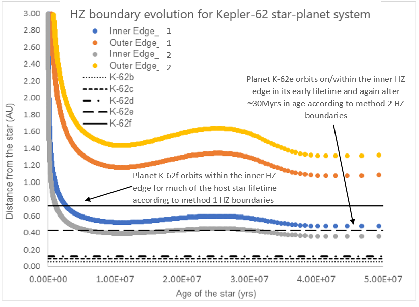
Potential future telescopes suitable for these recommendations would be the Habitable Exoplanet Imaging Mission (HabEx) and the Large Ultraviolet Optical Infrared Surveyor (LUVOIR) (Arney et al., 2018).
A major conclusion from the investigation of a 1 M⊙ hypothetical star reveals the potential for a closer inner HZ edge than formerly estimated (0.325 AU from the host star when albedo (A) = 0.9 in this work). The repercussions of this updated estimate imply that if a closely orbiting planet with a high albedo is found to orbit its host star, it may still be habitable and should not be neglected in terms of its habitability prospects. This also extends the frequency of habitable exoplanets if the inner edge of the HZ truly can exist at close proximity to the host star in question, having repercussions on exoplanet characterisation as a whole if these HZ distances can be replicated in subsequent works or verified by rocky exoplanet observations.
Furthermore, our results reinstate that a tidal-locking scenario is likely to shorten the width of the HZ significantly and draw it closer to the host star – introducing constraints for rocky bodies that may be considered habitable. This is significant when considering planets orbiting beyond the inner edge of the HZ and re-evaluation of their habitability may be necessary once atmospheric, albedo and other orbital data for exoplanetary systems can be determined.
Previous HZ publications have centred around MS habitability (Kasting et al., 1993; Kopparapu et al., 2013), yet the temporal evolution of the HZ is becoming more widely recognised as fundamental in evaluating habitability as a whole (Ramirez and Kaltenegger, 2014; Danchi and Lopez, 2013). Pre-MS evolution is a deciding factor as to whether planets are still habitable during the MS phase – planets within the pre-MS HZ are unchartered targets in the search for habitable worlds or even as tools to decipher habitable planet diversity and early water delivery mechanisms. Such results should be utilised as a first order estimation of exoplanetary habitability.
To summarise, there is still significant progress left to be made in calculating reliable HZ boundaries and to then characterise the habitability of planets orbiting within them. Nevertheless, these HZ boundaries serve as a critical basis for the assessment of the habitability of modelled exoplanetary systems. Such works are beneficial as they may result in the detection of habitable exoplanets suitable for observational follow-ups, or even to the eventuality of discovering evidence for extra-terrestrial life.
References:
- Arney, G., Batalha, N., Cowan, N., Domagal-Goldman, S., Dressing, C., Fujii, Y., Kopparapu, R., Lincowski, A., Lopez, E., Lustig-Yaeger, J. and Youngblood, A., 2018. The Importance of Multiple Observation Methods to Characterize Potentially Habitable Exoplanets: Ground-and Space-Based Synergies. arXiv preprint arXiv:1803.02926.
- Danchi, W.C. and Lopez, B., 2013. Effect of Metallicity on the Evolution of the Habitable Zone from the Pre-main Sequence to the Asymptotic Giant Branch and the Search for Life. The Astrophysical Journal, 769(1), p.27.
- Kasting, J., Whitmire, D. and Reynolds, R., 1993. Habitable Zones around Main Sequence Stars. Icarus, 101(1), pp.108-128.
- Kopparapu, R., Ramirez, R., Kasting, J., Eymet, V., Robinson, T., Mahadevan, S., Terrien, R., Domagal-Goldman, S., Meadows, V. and Deshpande, R., 2013. HABITABLE ZONES AROUND MAIN-SEQUENCE STARS: NEW ESTIMATES. The Astrophysical Journal, 765(2), p.131.
- Ramirez, R.M. and Kaltenegger, L., 2014. The habitable zones of pre-main-sequence stars. The Astrophysical Journal Letters, 797(2), p.L25.
How to cite: Hogan, J.: Characterising the Potential for Planetary Habitability: A Study of the Temporal Evolution of Exoplanet Habitable Zones, Europlanet Science Congress 2022, Granada, Spain, 18–23 Sep 2022, EPSC2022-369, https://doi.org/10.5194/epsc2022-369, 2022.
Short-period, low-mass planets have been found to often display inflated atmospheres [1]. Here, we investigate the interior structure of such planets with a moderate water budget using a fully self-consistent planet interior model [2, 3], where water can exist in supercritical state. This has been done by increasing the working range of an existing interior model, allowing us to explore the 0.2-2.3 Earth mass range. We consider planets with water mass fractions (WMF) ranging from 0.01% to 5% and irradiation temperatures between 500 and 2000K. Moreover, we consider three possible internal compositions; a pure rocky interior, an Earth-like core mass fraction (0.325) and a Mercury-like core mass fraction (0.7).
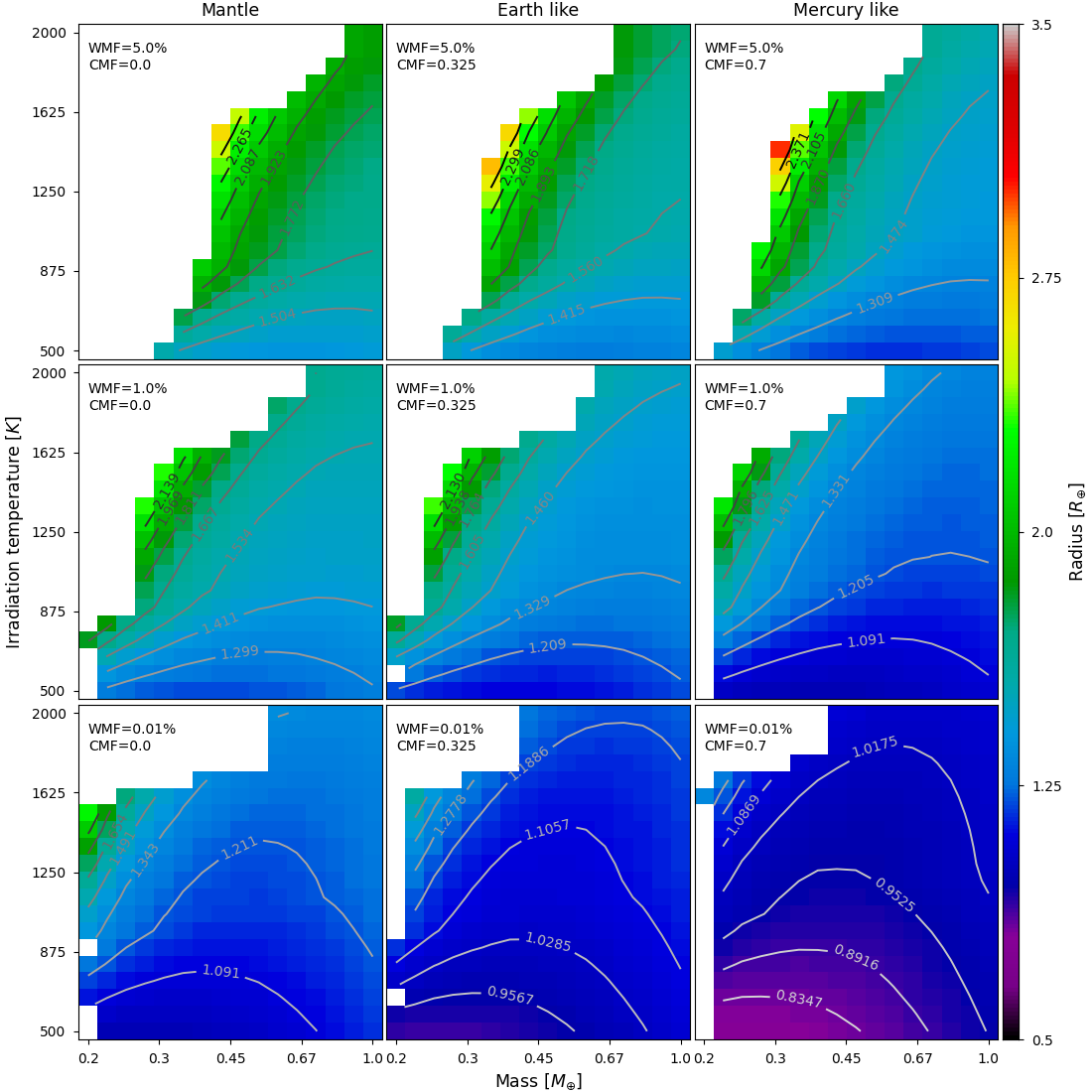
Figure 1: Computed planetary radii Rp at the transiting depth of 20mbar as a function of planetary mass and irradiation temperature. Columns correspond to different core mass fractions (0, 0.325, 0.7, from left to right) while rows correspond to different water mass fractions (5%, 1%, 0.01%, from top to bottom). Any missing data correspond to cases where the atmosphere is hydrostatically unstable.
We find that at higher masses, the planet radius increases with the planet mass, and the radii for planets with supercritical water are greater than if water was in a condensed phase. An important mass of water can also result in a notable compression of the refractory layers (up to 0.1 Earth radius for a WMF of 5%). At lower masses, we find that the steam atmosphere inflates, and becomes gravitationally unstable when the scale height of the atmosphere exceeds ~0.1 times the planetary radius. We propose to use this H/Rp ratio as a stability criterion for steam atmospheres.
Our data can be used to estimate the maximum WMF that can be retained by a planet given its mass, irradiation temperature and interior composition. For a given mass and temperature, a large part of the planets considered here can be stable even if constituted of 100% water. As the temperature increases or as the mass decreases, the surface gravity of a 100% water planet becomes too weak to retain the steam atmosphere. It is then possible to estimate the maximum WMF under which the atmosphere is stable.
Our results show that planets under 0.9 Earth masses should typically present unstable hydrospheres. We also find that a sharp transition exists between a planet able to hold a 100% water atmosphere and an unstable one, as the H/Rp stability criterion exceeds 0.1. Additionally, we note that this class of planets is a viable explanation of the current Super-Puff category without invoking instrumental limitations, as the mass of water molecules induces a more inflated atmosphere than H/He planets.
References:
[1] Turbet, M., Bolmont, E., Ehrenreich, D., et al. 2020, A&A, 638, A41
[2] Aguichine, A., Mousis, O., Deleuil, M., et al. 2021, ApJ, 914, 84
[3] Vivien, H.G., Aguichine, A., Mousis, O., et al. 2022, ApJ
How to cite: Vivien, H., Aguichine, A., Mousis, O., Deleuil, M., and Marcq, E.: Constraints on the existence of low-mass planets with supercritical hydrospheres, Europlanet Science Congress 2022, Granada, Spain, 18–23 Sep 2022, EPSC2022-418, https://doi.org/10.5194/epsc2022-418, 2022.
Convective mantle flow of terrestrial planets is governed by a temperature- and pressure-dependent rheology. This results in a stagnant-lid regime observed on most terrestrial planets. Plastic deformation can lead to breaking of the strong upper lithosphere, which resembles plate tectonics on Earth.
Most efforts to model mantle convection with self-consistent plate tectonics combine Newtonian power-law with a stress-dependent pseudo-plastic rheology.
In the uppermost mantle, where stresses are high, deformation is thought to be driven partly by dislocation creep. This is often neglected in viscoplastic consideration, which employ purely diffusion-creep-driven flow combined with a yield criterion.
In our models we employ an effective viscosity law combining both Newtonian and Non-Newtonian power laws with a pseudo-plastic model. We study the influence of rheology in combination with grain size and different yield stress parameterizations on the likelihood of the on-set of plate tectonics in a 2D-spherical annulus geometry. We compute common diagnostic values related to the characterization of a mobilized surface. With this model we aim at identifying key planetary factors for the occurrence or absence of plate tectonics.
How to cite: Henke-Seemann, O. and Noack, L.: Critical factors for plate tectonics on rocky planets, Europlanet Science Congress 2022, Granada, Spain, 18–23 Sep 2022, EPSC2022-585, https://doi.org/10.5194/epsc2022-585, 2022.
Benzene is the simplest organic compound with a 6-carbon aromatic ring. As such, it was used as a first order representative of aromatic compounds in planetary atmospheres. These compounds can be brought by asteroid impacts into rocky planetary atmospheres, where they can serve as precursors for further synthesis. Our experiments show that benzene vapours in nitrogen-dominated atmospheres subjected to asteroid impacts (modelled by laboratory laser shots) lead to the formation of acetylene and hydrogen cyanide. Both these products appear in many proposed mechanisms of prebiotic chemistry.
How to cite: Knížek, A. and Petera, L.: The stability of benzene in planetary atmospheres, Europlanet Science Congress 2022, Granada, Spain, 18–23 Sep 2022, EPSC2022-830, https://doi.org/10.5194/epsc2022-830, 2022.
Exoplanets in the mass range between Earth and Saturn show a large spread in radii/densities for a given planetary mass. The most approaches to explain this spread and the distribution of planetary properties therein can be split into two groups. The first considers the planetary formation paths as the primary mechanism shaping this distribution, and the second group considers the radius spread as a consequence of the atmospheric evolution driven by the atmospheric mass loss. The majority of the latter studies, however, consider only the observed radius spread with some theoretical underlying mass distribution, as for most of the Kepler planets the mass is unknown.
In this study, we examine the mass-radius distribution of the observed planets with masses between 1 and 108 Earth masses with the aim to understand to which extent it can be explained by the evolution of planetary atmospheres driven by thermal contraction and the hydrodynamic escape, and in which regions of the parameters state the initial parameters of planets set up by specific formation processes are critical for the final (gygayears old) state.
Our modeling framework accounts simultaneously for the realistic atmospheric mass loss by interpolating within the grid of upper atmosphere models and for the thermal evolution of planets by means of the MESA code. As the atmospheric mass loss on the long timescales is strongly affected by high energy stellar radiation, we also account for the whole range of different possible stellar evolution histories as represented by the Mors code.
We consider the grid of model planets in the mass range given above evolving at different orbital separations (corresponding to the equilibrium temperatures of ~500-1700 K) around the solar mass star. As initial parameters for our atmosphere evolution models, we adopt the predictions of the analytical approximations based on formation models (Mordasini 2020) and consider the two possible scenarios: planets formed in the inner disk (relatively small initial atmospheres) and beyond the snow line (large initial atmospheres) with consequent inward migration at the early phase of the planetary system evolution.
The whole radius spread predicted using this approach outlines well the observed distribution (including about 240 planets with mass and radius uncertainties below 45% and 15% respectively), except for a group of very close in (within ~0.1 AU) massive (~70-110 Mearth) planets with radii comparable to the Jupiter radius. The radii of these planets can not be reproduced by our models even by assuming the atmospheric mass fractions above 80% without some additional heating source. A strong correlation of the radii with equilibrium temperature (Rpl~Teq0.7) suggests that the inflation mechanism is similar to that of the so-called "inflated Jupiters", where a range of possible explanations was suggested including the tidal interaction with the host star, vertical heat transport towards the deep atmospheric levels or the Ohmic dissipation.
The more detailed analysis shows that the low-mass end of the mass-radius distribution (below 10-15 Earth masses) is dominated by the effect of the atmospheric mass loss (and thus extremely dependent on the activity evolution history of the host star) and weakly depend on the initial parameters, and thus, on the specific formation mechanism of the exoplanets. For more massive planets, though some of them can be significantly affected by the atmospheric mass loss, the initial conditions become important and the variability in the possible stellar histories can only explain about one fourth of the whole spread. Thus, for explaining the upper boundary of the spread above ~20 Mearth one needs to consider the voluminous initial atmospheres which can be explained by the formation at the large distance from the host star. However, the activity history of the host star can be theoretically resolved using the present-day radii of the companion planets for the significant fraction of planets with masses up to ~60 Mearth.
Finally, the detailed comparison between the model predictions and the observations within different Teq intervals reveals a relatively small (~6%) but a presumably systematic group of the outliers with radii considerably smaller than the lower boundary predicted by our models for Teq<~800 K. Assuming the hydrogen dominated atmospheres surrounding rocky cores, these planets would not have more than ~1% of their mass in the envelope, while for their masses (>10 Mearth) the accretion models predict the initial atmospheric mass fraction order of 10%, and the total atmospheric mass loss throughout the evolution according to our models is insufficient to remove this much of the atmospheric material. This suggests, that the formation mechanisms and structures of these planets are considerably different from our assumption of the hydrogen-dominated atmospheres accreted onto the rocky core.
How to cite: Kubyshkina, D. and Fossati, L.: Mass-radius relation of intermediate-mass planets outlined by the hydrodynamic escape of planetary atmospheres and formation, Europlanet Science Congress 2022, Granada, Spain, 18–23 Sep 2022, EPSC2022-1089, https://doi.org/10.5194/epsc2022-1089, 2022.
Rocky (exo)planets can be classified based on their mantle viscous state. The mantle viscosity influences the efficiency of convection and heat loss of the planet, altering the outgassing rate. Low viscous planets are hypothesized to have strong volcanic activity reshaping the surface and changing the atmosphere. This can be seen in other almost-similar rocky bodies such as Io, one of Jupiter’s Galilean moons, and would be expected of young rocky exoplanets. Whereas, the intermediate viscous planets have less vigorous resurfacing. They experience occasional complete mantle-overturn to slow-moving plate tectonics driven by mantle convection. As a result, their atmospheres vary little or smoothly across time. High viscous planets can be seen as inert, with little or no mantle convection. Moreover, hotspot volcanism might still occasionally contribute to outgassing, producing a less dominant atmosphere. Through this relationship, a planet’s atmosphere could reveal information about the evolution of a planet's interior and surface. However, we rely on primary observables to characterize (exo)planets. So, is there a correlation between a planet's orbital position and mantle viscosity? The answer to this question would aid in the characterization of rocky exoplanets, which is the focus of this work.
To study the relationship between a planet’s mantle viscous state, interior composition, and structure. We use Perple-X to generate mineral physics properties, and Burnman to build a 1-dimensional depth profile of the planet. From this, 2-dimensional annulus compressible convection models are developed using ASPECT. And, exploring the stagnant lid, the episodic lid, and the tectonic convection regimes. We consider the anelastic liquid approximation (ALA), and the truncated anelastic liquid approximation (TALA) formulations. An isoviscous profile results in a hot mantle but can be used for first-order approximations of mantle dynamics without a crust. However, the presence of crust requires for temperature-dependent stratified viscosity profile for the deeper mantle to allow for the cooling of the mantle. The stratification structure of the mantle is determined by the temperature sensitivity of the mineral phases present in the depth profile of the mantle. The iron mass fraction of the planet, which is highly dependent on the orbital position dictates the thermal state of the given planet. Moreover, a high mass iron fraction in the mantle results in a highly viscous planet. Which cools much faster but with a higher average temperature in the earlier phases of evolution. And vice versa to a similar mantle state with less iron mass fraction in the mantle.
How to cite: Adhiambo, V., Root, B., and Desert, J.-M.: Rocky worlds: What do a planet's orbital parameters tell us about its mantle state?, Europlanet Science Congress 2022, Granada, Spain, 18–23 Sep 2022, EPSC2022-1219, https://doi.org/10.5194/epsc2022-1219, 2022.
EXOA5 | Devolatilization During Rocky (Exo)planet Formation: Mechanisms, Simulations, and Observations
The growth of dust grains to dust aggregates is a very important process in the chain of events from dust to planetesimals in protoplanetary discs (PPDs). Not only the size, shape, and porosity play an important role in the collisional growth process, but also the collision speed, the type of gas coupling and the charge of the dust particles [1, 2].
The ICAPS (Interactions in Cosmic and Atmospheric Particle Systems) campaign provides an experimental approach to protoplanetary dust growth and all the above parameters under realistic PPD conditions. The first ICAPS experiment flew onboard the TEXUS-56 sounding rocket and consisted of a vacuum chamber with a cloud of micrometer-sized SiO2 spheres embedded in a rarefied gas inside. The dust particles could be manipulated using temperature and external electric fields. During flight, the particles were observed using two overview cameras and a high-speed camera attached to a long-distance microscope. In total, three electrical scans were conducted to measure the charge distribution of the dust particles. Two of these scans (E1, E3) were applied immediately after the two dust injections, while a longer one (E2) was performed after the Brownian growth phase. Each of these scans consisted of two equal-length phases of different field polarisation. The analysis of the image recordings provided precise particle tracks and velocities as well as the mass and size of the dust aggregates [3]. From the change in velocity, when the external electric field was present, it was also possible to derive the particle charge.

Fig.1: Charge per monomer plotted against the cumulative normalized frequency of tracked particles during the electrical scans immediately after the first dust injection (E1), after the Brownian motion phase (E2), and after the second injection (E3), respectively. The duration between E1 and E2 was 164s. In this period, the mean charge per monomer grain decreased to less than 40% of the initial value.
In Fig. 1, the electric charge per monomer grain is plotted as a cumulative normalized frequency distribution of all particles tracked during each scan. Over the duration of 164 s between E1 and E2, a reduction of the mean charge per monomer grain to less than 40% of the initial value was observed. This finding is an indication that there was a relatively large number of distributed charges immediately after the injection, which allowed rapid agglomeration due to the charge-enhanced collision cross-section. At a later stage of the experiment run, the agglomeration was likely mainly driven by Brownian motion and dipole-dipole interactions. It is planned that the evolution of grain charging during agglomeration will be explored in more detail as part of the Laplace campaign, which will use a similar setup for a variety of experiments on the ISS.
References
[1] Blum, J., “Dust agglomeration”, Advances in Physics, vol. 55, pp. 881–947, 2006. doi:10.1080/00018730601095039.
[2] Güttler, C., Blum, J., Zsom, A., Ormel, C. W., and Dullemond, C. P., “The outcome of protoplanetary dust growth: pebbles, boulders, or planetesimals?. I. Mapping the zoo of laboratory collision experiments”, Astronomy and Astrophysics, vol. 513, 2010. doi:10.1051/0004-6361/200912852.
[3] Schubert, B., “ICAPS Sounding Rocket - Particle Growth”, 2020. doi:10.5194/epsc2020-567.
How to cite: Molinski, N., Pöppelwerth, A., Schubert, B., Schräpler, R., von Borstel, I., Houge, A., Krijit, S., Balapanov, D., Vedernikov, A., and Blum, J.: ICAPS: Charge effects in dust agglomeration experiments – Results from the TEXUS-56 sounding rocket flight, Europlanet Science Congress 2022, Granada, Spain, 18–23 Sep 2022, EPSC2022-377, https://doi.org/10.5194/epsc2022-377, 2022.
The ICAPS experiment (Interactions in Cosmic and Atmospheric Particle Systems) was part of the Texus-56 sounding rocket flight in November of 2019. ICAPS studies the agglomeration of 1.5 µm-sized, monomeric silica grains under microgravity conditions, as would be present in the early stages of dust growth in protoplanetary disks, which our study aims at describing.
For this, a cloud of dust was injected into a vacuum chamber with ~7000 monomer grains per mm³. A thermal trap was then utilized to stabilize the dust cloud against any external disturbances during the flight. Two overview cameras and a long-distance microscope with a high-speed camera were used for the in-situ observations of the particles (see Figs. 1 and 2).
This talk focuses on the data analysis and results of ICAPS, in particular with respect to Brownian motion and aggregate growth. From the total experiment time of six minutes of almost perfect weightlessness, we extracted the masses and translational friction times of 414 dust aggregates from their translational Brownian motion. For a subset of 69 of these particles, we were also able to derive their moments of inertia and rotational friction times from their Brownian rotation. With these data, we derived a fractal dimension close to 1.8 for the ensemble of dust aggregates. We compared this unambiguous physical method for the determination of the fractal dimension with an optical approach, in which the mass is derived through the particle extinction and the moment of inertia is derived from the microscopic images.
The combination of both methods then facilitates the growth analysis, for which the overview cameras were also used. We observed an initial rapid, charge-induced growth of aggregates, which was followed by a slower growth rate, which was dominated by ballistic cluster-cluster agglomeration. As a surprise, around 100 seconds into the flight, clear indication for runaway growth (or the onset of gelation) was observed.

Fig. 1: Examples of dust aggregates from the long-distance
microscope images.
Fig. 2: Image from one of the overview cameras after 100 s of experiment time (1024 x 768 pixels, about 12 x 9 mm²).
How to cite: Schubert, B., Molinski, N., Blum, J., Glißmann, T., Pöppelwerth, A., von Borstel, I., Balapanov, D., Vedernikov, A., Houge, A., and Krijt, S.: ICAPS: Dust aggregate properties and growth derived from Brownian translation and rotation from the ballistic to the diffusive limit, Europlanet Science Congress 2022, Granada, Spain, 18–23 Sep 2022, EPSC2022-581, https://doi.org/10.5194/epsc2022-581, 2022.
In order to form a rocky, potentially habitable planet, like Earth, the planet’s building blocks must loose volatiles. White dwarfs that have accreted planetary material provide the perfect opportunity to study the volatile content of planetary building blocks. The unique behaviour of Mn and Na depending on the conditions under which volatiles are lost means that planetary material in the atmospheres of white dwarfs can tell us how planetary building blocks lost volatiles [1]. This talk will summarise some recent results regarding observations of volatiles in the atmospheres of white dwarfs, models that describe how white dwarfs accrete volatiles and evidence from white dwarfs for volatile loss both early, in the hot, inner regions of a planet-forming disc and late, when large-scale melting is induced following impacts.
How to cite: Brouwers, M., Bonsor, A., Harrison, J., Shorttle, O., and Malamud, U.: How do planetary bodies lose volatiles?, Europlanet Science Congress 2022, Granada, Spain, 18–23 Sep 2022, EPSC2022-1223, https://doi.org/10.5194/epsc2022-1223, 2022.
EXOA6 | Exoplanet observations, modelling and experiments: Characterization of their atmospheres
The atmospheres of sub-Neptunes are expected to exhibit considerable chemical diversity, beyond what is anticipated for gas-giant exoplanets. Recently, in Guzman-Mesa et al 2022 we constructed self-consistent radiative transfer and equilibrium chemistry models to explore this chemical diversity. We use GJ 436 b as a case study to further study joint atmosphere-interior models. In particular, we constrain the properties of the interior and atmosphere of the planet based on the available Spitzer measurements. While it is possible to fit the emission spectrum of GJ 436 b using a high-metallicity model, we demonstrate that such an atmosphere is inconsistent with physically plausible interior structures. It remains the case that no existing study can adequately fit the 4.5-micron Spitzer secondary eclipse measurement, which is probably caused by chemical disequilibrium. In the light of the recently-launched JWST, we recommend that future analysis of emission and transmission spectra of sub-Neptune planets are carried out self-consistently using both the atmospheric and interior structure models.
How to cite: Guzmán Mesa, A.: Chemical diversity of the atmospheres and interiors of sub-Neptunes, Europlanet Science Congress 2022, Granada, Spain, 18–23 Sep 2022, EPSC2022-25, https://doi.org/10.5194/epsc2022-25, 2022.
Ground-based high-resolution spectroscopy allows us to probe the chemical composition and atmospheric dynamics of hot jupiters through the Cross-Correlation Function method. This requires however careful data processing and development of analysis tools in order to extract such a faint exoplanetary signal from the overwhelming telluric and stellar contributions. With a high spectral resolution power of 70,000 and a large continuous spectral range between 0.9 and 2.5 microns, the near-infrared spectro-polarimeter SPIRou on the CFHT is a powerful instrument for exoplanet atmosphere characterization since its first light in 2018. I will present our analysis of SPIRou primary transit observations of some short-period exoplanets. Preliminary results regarding the detection of the metastable He triplet and molecules in the hot jupiters HD 189733b and HD 20458b, the warm neptunes GJ 3470b and Au Mic b, the mini neptune GJ 1214b, the hot neptune WASP-127b, and the warm saturn WASP-69b, will be presented.
Figure 1: Cross correlation between observed and synthetic spectra of HD189733b (expressed in S/N ratio) calculated over a grid of velocity parameters Kp (radial velocity semi-amplitude) and V0 (additional Doppler shift of atmospheric lines at mid-transit). The correlation is maximum at the expected position in this parameter space [1]. The model spectra include water vapor as the only molecular absorber.
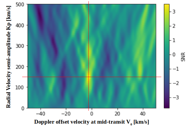
References :
[1] Boucher, A., Darveau-Bernier, A., Pelletier, S., Lafrenière, D., Artigau, E., et al., (2021). Characterizing Exoplanetary Atmospheres at High Resolution with SPIRou: Detection of Water on HD 189733 b. The Astronomical Journal, American Astronomical Society, 162 (6), pp.233.
How to cite: Masson, A., Vinatier, S., Bezard, B., and Team, A.: Characterizing exoplanetary atmospheres with SPIRou, Europlanet Science Congress 2022, Granada, Spain, 18–23 Sep 2022, EPSC2022-446, https://doi.org/10.5194/epsc2022-446, 2022.
We recreate a Titan-like climate using an Earth-like global climate model (GCM) by varying a small set of planetary parameters. Understanding the range of possible climate states for Earth-like planets is important for interpreting exoplanet observations and Earth’s own climate history. We find that simply reducing the available water at the surface does not fully reproduce Titan-like conditions. This may indicate that there are many possible “in-between” states an Earth-like planet can have that span the gap between the Earth and Titan climate archetypes. We use three observationally motivated criteria to determine Titan-like conditions: 1) the peak in surface specific humidity is not at the equator, despite it having the warmest annual-mean temperatures (Ádámkovics et al. 2016); 2) the vertical profile of specific humidity in the equatorial column is nearly constant through the lower troposphere (Niemann et al. 2005); and 3) the relative humidity near the surface at the equator is significantly lower than saturation (lower than 60%; Niemann et al. 2005; Tokano et al. 2006). We first limit the available water by placing a continental land strip centered on the equator and varying its width. This mimics Titan’s dry tropics and wet poles, and could be similar to past continental arrangements in Earth’s history. Land strips alone allow some experiments to meet two Titan-like criteria, but none show the near-constant vertical profile of specific humidity. We take three of these land strip widths and vary the rotation period, starting with Earth’s rotation and moving towards Titan’s (16 Earth days). Slowing the rotation results in fewer experiments meeting any of the Titan-like criteria due to increased access to oceanic moisture from the widened Hadley Circulation. For the same three land strip widths and using Earth rotation, we vary the volatility of the condensable via a constant multiplied to the saturation vapor pressure. Titan’s condensable, methane, is more volatile under Titan’s surface conditions than water is on Earth, resulting in high specific humidities. By artificially increasing the saturation vapor pressure, we can approximate this effect without changing the properties of the condensable. Experiments with a volatility constant of 2.5 (the maximum used in this work) meet all three Titan-like criteria, demonstrating that an Earth-like planet can display Titan-like climatology by changing only a few physical parameters.
How to cite: McKinney, M. and Mitchell, J.: Dune, Waterworld, and Everything in-between: Creating a Titan-like Climate on an Earth-like Planet, Europlanet Science Congress 2022, Granada, Spain, 18–23 Sep 2022, EPSC2022-742, https://doi.org/10.5194/epsc2022-742, 2022.
Motivation
Photochemical hazes are expected to form in the atmospheres of many hot Jupiters, especially those with equilibrium temperatures near 1,200 K (like HD 189733b) and below. Heating and cooling from photochemical hazes can strongly impact temperature structure and atmospheric circulation but has previously been neglected in 3D general circulation models (GCMs) of hot Jupiters.
Methods
We present 3D simulations of hot Jupiter HD 189733b that include radiative feedback from photochemical hazes. Hazes were simulated as radiatively active tracers with a constant particle size of 3 nm. For the nominal simulations, a complex refractive index of soot was assumed. To examine how the results depend on the choice of the refractive index, we also performed additional simulations with a refractive index of Titan-type hazes.
Effect on atmospheric circulation
The response of atmospheric circulation to heating and cooling by hazes strongly depends on the assumed haze refractive index. For simulations with soot-like hazes, the equatorial jet broadens and slows down (Fig. 1, center panel). At low pressures, the day-to-night component of the flow strengthens. Vertical velocities increase. The horizontal haze mixing ratio distribution (Fig. 2) remains relatively similar to simulations without haze radiative feedback, with particularly high haze abundances near the morning terminator (as also seen in Steinrueck et al., 2021). For simulations with Titan-type hazes, the equatorial jet instead accelerates and extends to lower pressures (Fig. 1, right panel). This results in a substantially different 3D distribution of hazes, with hazes being most abundant at the dayside, the evening terminator and the equatorial region around the planet. This means that circulation, thermal structure, and haze distribution depend strongly on the assumed haze composition and optical properties.
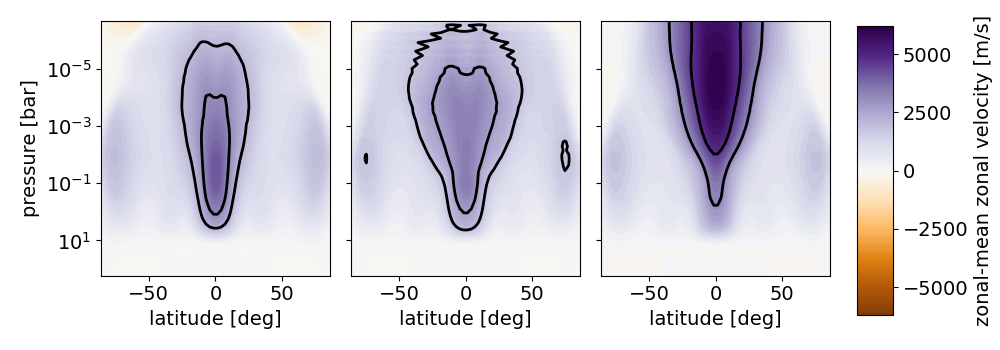
Fig. 1: Zonal-mean zonal velocity in a simulation without haze radiative feedback (left), with soot-like hazes (center) and with Titan-type hazes (right). Black contours highlight the regions in which the zonal-mean zonal velocity is larger than 50% and 75% of its peak value within the simulation. The haze production rates are identical for both simulations with haze radiative feedback (2.5x10⁻¹¹ kg/m2/s).
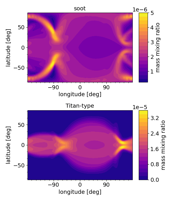
Fig. 2.: Haze mass mixing ratio at the 0.1 mbar level in a simulation with soot-like hazes (left) and with Titan-type hazes (right). The substellar point is located at the center of each panel. Both simulations shown have a haze production rate of 2.5x10⁻¹¹ kg/m2/s at the substellar point.
Effect on temperature structure and emission spectra
In all simulations with haze radiative feedback, strong thermal inversions appear at low pressures on the dayside (Fig. 3). In the soot-like case, two distinct thermal inversions form, separated by a temperature minimum below the haze production region. This additional structure is not seen in 1D simulations. It is caused by upwelling on the dayside transporting air with low haze abundance upwards, resulting in a local minimum in the haze number density below the production region. Deeper regions of the atmosphere (p>100 mbar) cool compared to simulations without hazes.
The altered temperature structure leads to changes in emission spectra (Fig. 4): The amplitude of the near-infrared water features decreases in simulations with haze radiative feedback. At wavelengths > 4 µm, the emitted flux increases. Because thermal inversions caused by photochemical hazes peak at much lower pressures than the regions probed by existing low-resolution observations, current observations of HD 189733b neither confirm nor rule out such a temperature inversion.

Fig. 3: Dayside temperature profiles, calculated using an average weighted by the cosine of the angle of incidence
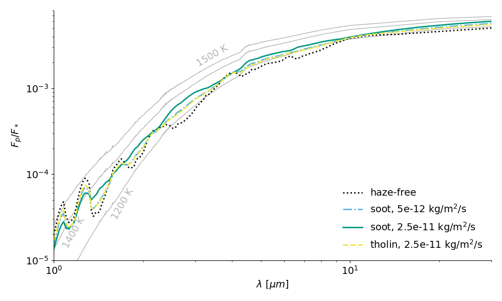
Fig. 4: Dayside emission spectra. For comparison, blackbody spectra are shown as thin gray lines.
References:
Steinrueck, M. E., A. P. Showman, P. Lavvas, T. Koskinen, X. Tan, and X. Zhang (2021). MNRAS, 504(2), pp. 2783-2799. doi:10.1093/mnras/stab1053.
How to cite: Steinrueck, M., Koskinen, T., Parmentier, V., Lavvas, P., Tan, X., and Zhang, X.: Photochemical hazes dramatically alter temperature structure and atmospheric circulation in 3D simulations of hot Jupiters, Europlanet Science Congress 2022, Granada, Spain, 18–23 Sep 2022, EPSC2022-763, https://doi.org/10.5194/epsc2022-763, 2022.
Water-rich planets should be ubiquitous in the universe, and could represent a notable fraction of the sub-Neptune population. Among the detected exoplanets that have been characterized as sub-Neptunes, many are subject to important irradiation from their host star. As a consequence, hydrospheres of such planets are not in condensed phase, but are rather in supercritical state, with steam atmospheres on top. Such irradiated ocean planets (IOP) are good candidates to explain the distribution of masses and radii in the sub-Neptune category of exoplanets [1].
Here, we present the IOP model that computes the structure of water-rich planets that have high irradiation temperatures. The IOP model [2] combines two models in a self-consistent way: one for the interior structure, and one for the steam atmosphere. The interior structure model [3] contains several refractory layers (iron core and rocky mantle), and on top of them an hydrosphere with an up to date equation of state (EOS) with a validity range that extends to the plasma regime. The atmosphere model [4] connects the top of the interior model with the host star by solving equations of radiative transfer.
Our model has been applied to the GJ 9827 system as a test case and indicates Earth- and Venus-like interiors for planets b and c, respectively. Planet d could be an irradiated ocean planet with a water mass fraction of ∼20 ± 10%. We also compute mass-radius relationships for IOP and their analytical expression, which can be found in [2]. This allows one to directly retrieve a wide range of planetary compositions, without the requirement to run the model.
Due to their high irradiation temperatures, sub-Neptunes are expected to be subject to strong atmospheric escape. This supports the idea that a massive hydrosphere could be the remnant of a complete loss of an H-He envelope. The stability of hydrospheres themselves is discussed as well [5].
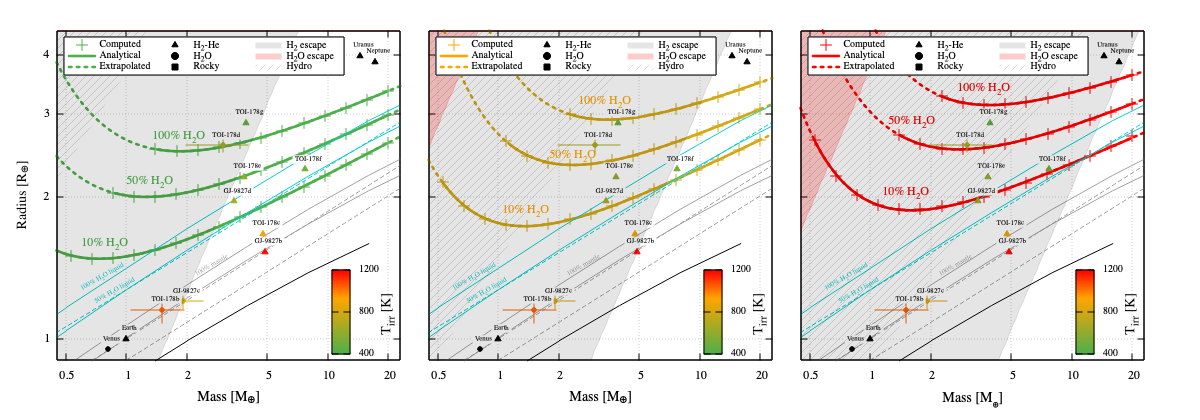
Figure 1. Mass-radius relationships produced by our model (green, yellow and red thick lines) [2], compared to mass-radius relationships of planets with only condensed phases and no atmosphere (black, grey and light blue thin lines). A few planets of the solar system, the GJ-9827 system and the TOI-178 system are represented as well. Shaded regions correspond to important atmospheric loss by Jeans escape (H and H2O), or hydrodynamic escape.
[1] Mousis, O., Deleuil, M., Aguichine, A., et al. 2020, ApJL, 896, L22.
[2] Aguichine, A., Mousis, O., Deleuil, M., et al. 2021, ApJ, 914, 84A.
[3] Brugger, B., Mousis, O., Deleuil, M., et al. 2017, ApJ, 850, 93.
[4] Marcq, E., Baggio, L., Lefèvre, F., et al. 2019, Icarus, 319, 491M.
[5] Vivien, H., Aguichine, A., Mousis, O., et al. 2022, accepted in ApJ.
How to cite: Aguichine, A., Mousis, O., Deleuil, M., Marcq, E., and Vivien, H.: Interior structure and possible existence of irradiated ocean planets, Europlanet Science Congress 2022, Granada, Spain, 18–23 Sep 2022, EPSC2022-904, https://doi.org/10.5194/epsc2022-904, 2022.
The population of Earth-sized exoplanets in short orbital periods of a few Earth days around small mass stars has continuously increased over the past years [1 - 3]. A fraction of these planets has stellar irradiation levels closer to Venus than the Earth, suggesting that a Venus-like Climate is more likely on those exoplanets [4]. At the same time, their small size, combined with a close-in orbit and small radius of the host star (relatively small star-planet size ratio), makes these worlds the best targets for follow-up atmospheric studies. Furthermore, when the planet transits the host star, such as in the case of TRAPPIST-1 planets, transmission spectra become available, potentially expanding the understanding of the planets’ atmospheric composition [5, 6].
The James Webb Space Telescope will advance the atmosphere and Climate characterisation of nearby rocky exoplanets, including TRAPPIST-1 c [7, 8]. The field will expand with the support of upcoming ground-based observatories and space telescopes, such as the ESA/Ariel mission, scheduled for launch in 2029. The interpretation of the observables produced by these missions: reflection, thermal emission, and transmission spectra will need support from dedicated models and theoretical studies of exoplanetary atmospheres. In particular, 3D Global Climate Models (GCMs) are critical for interpreting the observable signal’s modulations. They provide synthetic top-of-the-atmosphere fluxes that can be disk-integrated as a function of the orbital phase. The spatial and temporal variability of these fluxes reflects the atmospheric variability of the simulated temperature and wind fields and provides insight into the large-scale circulation.
In this work, we use the Generic-GCM to simulate a possible Venus-like atmosphere on TRAPPIST-1 c, considered a benchmark for highly-irradiated rocky exoplanets orbiting late-type M-dwarf stars. The Generic-GCM has been originally developed at Laboratoire de Météorologie Dynamique for exoplanet and paleoclimate studies [9 - 11], and has been continuously improved thanks to the efforts of several teams (e.g., LAB, Bordeaux; LESIA, Paris; Observatoire astronomique de l'Université de Genève). The model uses a 3D dynamical core, common to all terrestrial planets, a planet-specific physical part, and an up-to-date generalised radiative transfer routine for variable atmospheric compositions. To simulate a Venus-like atmosphere as a possible framework for the atmospheric conditions in TRAPPIST-1 c, we took a series of assumptions: synchronous rotation, zero obliquity and eccentricity, a Venus-like, carbon dioxide dominated atmosphere with 92-bar surface atmospheric pressure, and a radiatively-active global cover of Venus-type aerosols. The overarching goal is twofold: (1) to study the large-scale atmospheric circulation of rocky exoplanets with similar stellar irradiations to Venus; and (2) to address the observational prospects by producing phase curves (reflection and emission) and transmission spectra.
The TRAPPIST-1 c first 3D modelling results indicate a strong equatorial zonal superrotation jet responsible for the advection of warm air masses from the substellar region towards the nightside hemisphere. The thermal phase curves have different amplitudes and orbital phases of peak emission depending on whether they are: (i) carbon dioxide absorption bands (e.g., 14.99-16.21 μm in Figure 1 (a)); or (ii) part of the continuum (e.g. 11.43-12.50 μm, in Figure 1 (a)). The corresponding OLR and temperature fields suggest different spectral bands sound different atmospheric levels. The carbon dioxide absorption bands sound mesospheric levels (p ~ 1 mbar), while the continuum spectral bands sound the cloud top (p ~ 37 mbar) (see Figure 1 (b-e)). We will explore and expand these initial results in the context of the thermal structure and large-scale circulation of TRAPPIST-1 c. Furthermore, we will provide transmission spectra of TRAPPIST-1 c based on the outputs from our simulations with the Generic-GCM.
Additionally, we will provide a parametric study focused on the response of the thermal structure, large-scale atmospheric circulation and predicted observables to the variation of several parameters: surface gravity and radius following mass-radius relationships, planetary rotation rate (e.g., 1:1 versus 2:1 and 3:2 spin-orbit resonances), and instellation.
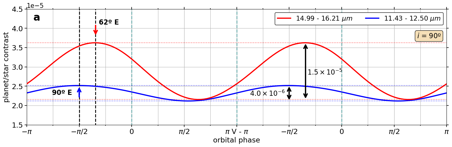
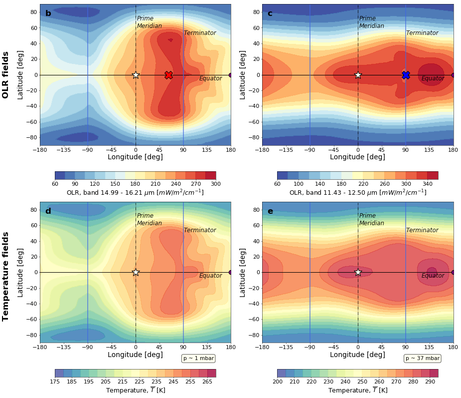
Figure 1. Relation between thermal phase curves, OLR and temperature fields and remote sensing of different TRAPPIST-1 c atmospheric levels. The two emission phase curves in panel (a) planet-to-star contrast as a function of the orbital phase, for an inclination 90º are: (i) 14.99-16.21 μm (solid red line); and (ii) 11.43-12.50 μm (solid blue line). The coloured arrows identify each phase curve peak emission's orbital phase and corresponding longitude, while the two head black arrows identify the amplitude of each phase curve. The green vertical dashed lines mark the orbital phases 0 and π, corresponding to eclipse and transit, respectively. Panels (b, c) represent the time-mean OLR fields in mW/m2/cm-1 (latitude vs. longitude) for the two selected phase curves. The red/blue cross mark the longitudinal location of the maximum peak emission over the equator. Panels (d, e) represent the time-mean temperature fields in K at two different pressure levels: p ~ 1 mbar (mesosphere) and p ~ 37 mbar (cloud top level), respectively. A white star (purple dot) identifies the substellar (antistellar) point. A solid (dashed) black line represents the equator (prime meridian), while the terminators are represented in solid blue lines. Data in all panels are time-averaged for ten orbits of TRAPPIST-1 c.
References:
[1] Gillon et al. 2017. Nature. 542.
[2] Zeichmeister et al. 2019. A&A. 627.
[3] Faria et al. A&A. 658.
[4] Kane et al. 2018. ApJ. 869.
[5] Lincowski et al. 2018. ApJ. 867
[6] Morley et al 2017. ApJ. 850
[7] JWST Proposal 2589 – Atmospheric reconnaissance of the TRAPPIST-1 planets https://www.stsci.edu/jwst/phase2-public/2589.pdf
[8] JWST Proposal 2304 – Hot Take on a Cool World: Does Trappist-1c Have an Atmosphere?
https://www.stsci.edu/jwst/phase2-public/2304.pdf
[9] Forget & Leconte, 2014. Phil. Trans R. Soc. A372.
[10] Turbet et al. 2016. A&A. 596. A112.
[11] Wordsworth et al. 2011. ApJL. 733. L48.
Acknowledgments
This work is supported by Fundação para a Ciência e a Tecnologia (FCT) through the research grants UIDB/04434/2020, UIDP/04434/2020, P-TUGA PTDC/FIS-AST/29942/2017
How to cite: Quirino, D., Gilli, G., Navarro, T., Turbet, M., Fauchez, T., Leconte, J., and Machado, P.: 3D Climate modelling of TRAPPIST-1 c with a Venus-like atmosphere and observational prospects, Europlanet Science Congress 2022, Granada, Spain, 18–23 Sep 2022, EPSC2022-1110, https://doi.org/10.5194/epsc2022-1110, 2022.
How to cite: Chakraborty, H. and Lendl, M.: Quantifying the impact of stellar activity on transmission spectroscopy for F,G and K type host-stars, Europlanet Science Congress 2022, Granada, Spain, 18–23 Sep 2022, EPSC2022-1181, https://doi.org/10.5194/epsc2022-1181, 2022.
EXOA7 | Future instruments to detect and characterise extrasolar planets and their environment
MAROON-X is a red optical EPRV spectrograph on the 8m Gemini North telescope that has been in regular science operations for the last two years. Depending on the amount of time available and the interests of the organizers, I could report on the current performance of the instrument, science results, future plans, and/or lessons learned. In terms of performance, the instrument continues to deliver radial velocity precision at the sub 30 cm/s level. We have found that many field M dwarfs have activity levels well below 1 m/s on short timescales, thus opening up the possibility of detecting very small planets on orbits out to the distance of the circumstellar habitable zone with intensive observational campaigns. I will report science results from a large, homogeneous follow-up program for TESS's M dwarfs, a blind search for planets around the nearest M dwarfs, and a selection of results from community use of the instrument. We will be upgrading the instrument with a laser frequency comb to improve the long-term calibration later this year. We also have the approval to install a solar telescope feed for the instrument. A key lesson learned is the importance of continual assessment and adjustment of the calibration (i.e., don't "set it and forget it") in the EPRV regime.
How to cite: Luque, R. and the MAROON-X instrument team: An update on MAROON-X, Europlanet Science Congress 2022, Granada, Spain, 18–23 Sep 2022, EPSC2022-90, https://doi.org/10.5194/epsc2022-90, 2022.
We will present a new instrument PLATOSpec which will be installed at E152 telescope at La Silla Observatory, Chile in 2023. PLATOSpec will be an echelle spectrograph with resolving power of 70000 capable of monitoring wavelength range from 380 to 680 nm with an expected accuracy in radial velocities around 3 m/s. PLATOSpec will have a blue sensitive chip, therefore, we will be able to provide a valuable information about the stellar activity. Main aims of PLATOSpec will be the ground based follow-up of currently TESS and later PLATO missions planetary candidates. We will be able to contribute mainly to detection and characterization of hot Jupiters and to discrimination of false positives and to determination of stellar parameters.
How to cite: Kabath, P., Vanzi, L., Hatzes, A., Guenther, E., Brahm, R., Janik, J., Minezaki, T., Skarka, M., and Karjalainen, R.: PLATOSpec a new spectrograph for the PLATO targets follow-up, Europlanet Science Congress 2022, Granada, Spain, 18–23 Sep 2022, EPSC2022-124, https://doi.org/10.5194/epsc2022-124, 2022.
In the past half-century, a new generation of successively ever larger and more sophisticated telescopes and instruments have ushered in a golden age of remarkable results in astronomy. This road is taking us to the age of the extremely large telescopes (ELTs). Riding on this wave and contributing to it is exoplanet research. We are characterising the orbit and mass of exoplanets with Doppler measurements which, combined with the transit technique provide estimates of bulk densities and compositions. The picture is completed with upcoming space missions such as ARIEL or PLATO. To prepare the road into this new era, we propose to build the MultiArray of Combined Telescope (MARCOT). This large aperture telescope consists of multiple identical low-cost telescopes, at a fraction of the cost of building an ELT. We propose MARCOT to support science cases, such as time-domain astronomy in general and exoplanet research in particular, that are too expensive or impractical to conduct on ELTs. MARCOT will be linked through optical fibres combined by a novel Multi-Mode Photonic Lantern (MM-PL) into a MM fibre that will feed a single high-resolution echelle spectrograph, optimized for extreme-precision radial velocity measurements. We will present the status of the project focusing on the work carried out towards the conceptual design and the prototype of MARCOT, which is being built at the CAHA Observatory (Almeria, Spain), to feed the CARMENES spectrograph.
How to cite: Amado, P., Aceituno, J., Pozuelos, F., and Ortíz, J. L.: MARCOT: A new approach to a large aperture telescope with a novel multimode photonic lantern, Europlanet Science Congress 2022, Granada, Spain, 18–23 Sep 2022, EPSC2022-312, https://doi.org/10.5194/epsc2022-312, 2022.
Technology now exists to enable large optical
systems that are capable of resolving and measuring faint sources not
accessible with current remote sensing instruments and detectors. The possibility
of creating ground-based telescopes at the 50m-scale with sufficient wavefront control
to both fully overcome the effects of the atmosphere, but with exquisite coronagraphic
capability starting at the telescope entrance pupil, means we may solve some of the most
fundamental cross-cutting scientific questions: like, "is there life outside of the solar system?".
The IAC is part of a consortium with the University of Hawaii and Universities in Lyon
to develop the technologies needed for the next generation telescopes aimed at direct
imaging of exoplanets around bright stars: the "ExoLife Finder (ELF)" telescope.
We have a detailed design for a 3.5-m diameter prototype, nicknamed Small-ELF, to
be built and installed at Teide Observatory by 2025. I will present the technological
and scientific challenges of such telescope.
How to cite: Lodieu, N., Kuhn, J., Moretto, G., Rebolo, R., Zhou, Y., Langlois, M., and Lewis, K.: Small-ELF: a propotype for the future ExoLife Finder hybrid optical telescope, Europlanet Science Congress 2022, Granada, Spain, 18–23 Sep 2022, EPSC2022-510, https://doi.org/10.5194/epsc2022-510, 2022.
The Twinkle Space Mission is a space-based observatory that has been conceived to measure the atmospheric composition of exoplanets, stars and solar system objects. The satellite is based on a high-heritage platform and will carry a 0.45 m telescope with a visible and infrared spectrograph providing simultaneous wavelength coverage from 0.5 - 4.5 μm. The spacecraft will be launched into a Sun-synchronous low-Earth polar orbit and will operate in this highly stable thermal environment for a baseline lifetime of seven years.
Twinkle will have the capability to provide high-quality infrared spectroscopic characterisation of the atmospheres several hundred bright exoplanets, covering a wide range of planetary types. Additionally, ultra-precise photometric light curves will accurately constrain orbital parameters, including ephemerides and TTVs/TDVs present in multi-planet systems.
Twinkle is available for researchers around the globe in two ways:
1) joining its collaborative multi-year survey programmes, which will observe hundreds of exoplanets and thousands of solar system objects; and
2) accessing dedicated telescope time on the spacecraft, which they can schedule for any combination of science cases.
I will present an overview of Twinkle’s capabilities and discuss the broad range of targets the mission could observe, demonstrating the huge scientific potential of the spacecraft. Furthermore, I will highlight the work of the Science Team of the Twinkle exoplanet survey, showcasing their science interests and the studies into Twinkle’s capabilities that they have conducted since joining the mission. Finally, I will discuss ongoing, and upcoming, early career programmes related to the Twinkle mission.
How to cite: Edwards, B., Wilcock, B., Joshua, M., Tessenyi, M., Stotesbury, I., Archer, R., and Barrathwaj Raman Mohan, Y.: The Twinkle Space Mission's Extrasolar Survey, Europlanet Science Congress 2022, Granada, Spain, 18–23 Sep 2022, EPSC2022-597, https://doi.org/10.5194/epsc2022-597, 2022.
Exoplanet observations with ground-based instruments are subject to climate conditions on Earth. Therefore, one important aspect in site selection for ground-based telescopes is the study of current climate conditions to optimise observing time. Since anthropogenic climate change is leading to a significant increase in global mean surface temperature, consequences for ground-based telescopes are likely [1], yet remain mostly unknown. The timescale needed to select the site and build a large telescope until its first light can easily take up more than a decade. In the case of the European Extremely Large Telescope, this process takes approximately 20 years. Together with a typical lifetime of 30 years for large telescopes, climate change potentially degrades site conditions assessed during the site selection process noticeably until end of lifetime.
We present a study of eight sites around the world where ground-based telescopes are already in operation. The selected sites are namely Mauna Kea on the island of Hawaii (USA), San Pedro Mártir in Baja California in Mexico, the three Chilean sites Cerro Paranal, Cerro Tololo and La Silla, La Palma on the Canary Islands (Spain), Sutherland in South Africa and Siding Spring in Australia. From the observatories hosting these telescopes, we collect in situ measurements of temperature, specific and relative humidity, precipitable water vapour, cloud cover and astronomical seeing. We compare these in situ measurements to the fifth generation atmospheric reanalysis (ERA5) of the European Centre for Medium-Range Weather Forecasts and score the agreement. A reanalysis is a global and continuous assimilation of observations combined with weather and climate modelling and provides a connecting link between measurements and global climate models (GCMs).
For a more holistic comparison and to study future trends, we use an ensemble of six of the highest resolution GCMs available with a horizontal grid spacing of 25-50 km. These GCMs are provided by the High-Resolution Model Intercomparison Project and developed as part of the EU Horizon 2020 PRIMAVERA project. We compare ERA5 climate output against historical GCM simulations and score their agreement. With this evaluation, we gain insights into the trustworthiness of future GCM simulations that were run up to 2050. Finally, we perform a Bayesian analysis of future trends.
We find that ERA5 provides a good representation since it agrees well with in situ measurements over most sites. The comparison between ERA5 and PRIMAVERA shows a good agreement for temperature, specific humidity and precipitable water vapour, for which we find increasing future trends leading to a deteriorating quality of astronomical observations. For relative humidity, cloud cover and astronomical seeing, the confidence in future trends projected by the GCMs is low, due to an inadequate representation of climate conditions in comparison to ERA5. Also, the trends found for these variables are not significant.
With this study, we show that climate change should be considered an important aspect of instrumentation design for ground-based telescopes, especially for high-contrast imaging observations.
References:
[1] Cantalloube, F., Milli, J., Böhm, C. et al. The impact of climate change on astronomical observations. Nature Astronomy 4, 826–829 (2020).
How to cite: Haslebacher, C., Demory, M.-E., Demory, B.-O., Sarazin, M., and Vidale, P. L.: Climate change drives degradation of future observations with ground-based telescopes, Europlanet Science Congress 2022, Granada, Spain, 18–23 Sep 2022, EPSC2022-791, https://doi.org/10.5194/epsc2022-791, 2022.
Ariel, the Atmospheric Remote-sensing Infrared Exoplanet Large-survey, was adopted as the fourth medium-class mission in ESA's Cosmic Vision programme to be launched in 2029. During its 4-year mission, Ariel will study what exoplanets are made of, how they formed and how they evolve, by surveying a diverse sample of about 1000 extrasolar planets, simultaneously in visible and infrared wavelengths. It is the first mission dedicated to measuring the chemical composition and thermal structures of hundreds of transiting exoplanets, enabling planetary science far beyond the boundaries of the Solar System. The payload consists of an off-axis Cassegrain telescope (primary mirror 1100 mm x 730 mm ellipse) and two separate instruments (FGS and AIRS) covering simultaneously 0.5-7.8 micron spectral range. The satellite is best placed into an L2 orbit to maximise the thermal stability and the field of regard. The payload module is passively cooled via a series of V-Groove radiators; the detectors for the AIRS are the only items that require active cooling via an active Ne JT cooler. The Ariel payload is developed by a consortium of more than 50 institutes from 16 ESA countries, which include the UK, France, Italy, Belgium, Poland, Spain, Austria, Denmark, Ireland, Portugal, Czech Republic, Hungary, the Netherlands, Sweden, Norway, Estonia, and a NASA contribution.
This presentation provides an overall summary of the science and instrument design for Ariel and presents the many activities that the Ariel team have planned to engage the science community at large and the public prior to launch. These include the Ariel Dry-Run program and citizen-science programs such as ExoClock and the Ariel Data Challenges.
How to cite: Tinetti, G., Eccleston, P., Lueftinger, T., Salvignol, J.-C., Fahmy, S., and Alves de Oliveira, C. and the Ariel team: Ariel: Enabling planetary science across light-years, Europlanet Science Congress 2022, Granada, Spain, 18–23 Sep 2022, EPSC2022-1114, https://doi.org/10.5194/epsc2022-1114, 2022.
Tartu Observatory telescopes offer unique guaranteed access to objects in the Northern hemisphere. The observational facilities include a 1.5- m and 0.6-m classic Cassegrain reflectors, and 0.31-m remotely controllable telescope .
The 1.5 m telescope is currently equipped with a long-slit Cassegrain spectrograph used for stellar characterisation. Historically, the objects of interest have been massive stars but we are now developing new research direction and expanding the list of targets to exoplanet- and disk-hosting stars.
We have started evaluating our capabilities to characterise host stars spectroscopically to determine their parameters and composition. In 2020, we carried out a pilot study of a TESS candidate planet host, which we found to have a rare, strong chemical peculiarity [1]. This also allowed us to prepare our tools, workflow, and end-to-end analysis. We are also contributing to the European Space Agency Ariel space mission by offering stellar activity monitoring.
The 0.6-m and 0.31-m telescopes are utilised for photometric measurements and the 0.31-m one in particular has been a workhorse for exoplanet transit monitoring. Since 2020, we have made significant preparations to develop and prove our transit observation capabilities: we have observed more than 70 transit light curves. About half of them have been submitted to ExoClock to contribute to Ariel mission planning.
Concerning future upgrades, Tartu Observatory will have new instruments by the middle of 2023. The upgrades include procuring a medium resolution echelle spectrograph (projected bandwidth 390 nm to 750 nm, R= 25 000) and new photometer (Johnson-Cousins BVRI and SDSS filters) for the 1.5-m telescope, which will not only enhance our capabilities in both spectroscopic and photometric data retrieval of host stars. In addition, a new remote control system of the telescope will be installed and improvements on instrumentation for the 0.6-m and 0.31-m photometric telescopes will be made.
This presentation will give an overview of our facilities, and of current and future spectroscopic and photometric capabilities.
References:
- “A rare phosphorus-rich star in an eclipsing binary from TESS”, Colin P. et al., A&A 658 A105 (2022), DOI: 10.1051/0004-6361/202142124
How to cite: Ramler, H., Kama, M., Folsom, C., Aret, A., and Eenmäe, T.: Observational Facilities and Stellar Characterization Capabilities at Tartu Observatory, Europlanet Science Congress 2022, Granada, Spain, 18–23 Sep 2022, EPSC2022-1149, https://doi.org/10.5194/epsc2022-1149, 2022.
EXOA9 | Towards better understanding planets and planetary systems diversity
With the swift advance in exoplanet sciences it is now possible to characterize not only the fundamental parameters (mass and radius) of planets but also their interior structure and bulk composition. The former is known to influence on the habitability conditions of terrestrial planets, and the latter in itself is a key aspect to understand planet formation processes and the origin of their diversity.
In order to accurately assess planetary internal composition, the derivation of the chemical abundances of the host stars is of extreme importance. In particualr, stellar abundances of Fe, Si, Mg are proposed as principal constraints to reduce degeneracy in exoplanet interior structure models under assumption of identical composition of these elements in the rocky planets and their host stars.
This regularly used assumption is based on our knowledge that stars and planets form from the same primordial gas and dust cloud. It is also supported by our Solar System observations for which we know that the composition of major rock forming elements (such as Mg, Si, and Fe) in the meteorites and telluric planets (with the exception of Mercury) is similar to that of the Sun. However, direct observational evidence for the aforementioned assumption for exoplanets is absent.
By using the largest possible sample of precisely characterized low-mass planets and their host stars, we show that the composition of the planet building blocks indeed correlates with the properties of the rocky planets (see Fig. 1). We also find that on average the iron-mass fraction of planets is higher than that of the primordial values, owing to the disk-chemistry and planet formation processes. Additionally, we show that super-Earths and super-Mercuries appear to be distinct populations with differing compositions, implying differences in their formation processes. We suggest that giant impact alone is not responsible for the high-densities of super-Mercuries.
I propose an oral contribution to speak about these very recent results published in Scinece.

Fig. 1 The iron-mass fraction of the planets inferred from the planets' mass and radius as a function of the iron-mass fraction of the protoplanetary disk, estimated from the host star abundances. Super-Mercuries (in brown) and super-Earths (in blue) appear as two distinct groups.
How to cite: Adibekyan, V., Dorn, C., Sousa, S., Santos, N., Bitsch, B., Israelian, G., Mordasini, C., Barros, S., Delgado Mena, E., Demangeon, O., Faria, J., Figueira, P., Hakobyan, A., Osagh, M., Soares, B., Kunitomo, M., Takeda, Y., Jofré, E., Petrucc, R., and Martioli, E.: Diversity of terrestrial planets: a link to the chemical makeup of their host stars, Europlanet Science Congress 2022, Granada, Spain, 18–23 Sep 2022, EPSC2022-74, https://doi.org/10.5194/epsc2022-74, 2022.
Planets smaller than Neptune are ubiquitous in the Galaxy and those around M stars constitute the bulk of warm and temperate worlds amenable for detailed atmospheric characterization. In this talk, we present a re-analysis of all the available data on small transiting planets around M dwarfs, refining their masses and radii (Luque & Pallé 2022, in press). Our precisely characterized sample reveals that this population is well described by only three discrete planet density populations, with bulk densities centered at 1.0, 0.5 and 0.24 relatively to Earth's. The first are rocky planets, the second are water worlds, and the third are puffy planets with Neptune-like densities. This density classification offers a much better insight to disentangle planet formation and evolution mechanisms, which are degenerate when using a radius-based classification. Our results are at odds with atmospheric mass loss models aiming to explain the bimodal radius distribution and suggest that the gap separates dry from water worlds rather than rocky planets with or without H/He envelopes. Formation models including type I migration explain naturally the observations independently of the accretion mechanism: rocky planets form within the snow line, water worlds form beyond and later migrate inwards. These results are to be published in Science and are currently under embargo.
How to cite: Luque, R. and Pallé, E.: On the nature of small planets orbiting low-mass stars, Europlanet Science Congress 2022, Granada, Spain, 18–23 Sep 2022, EPSC2022-89, https://doi.org/10.5194/epsc2022-89, 2022.
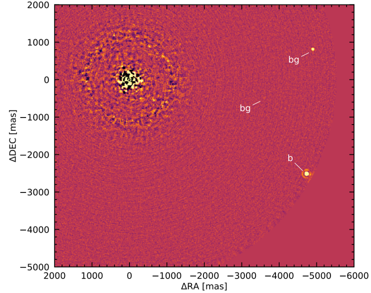
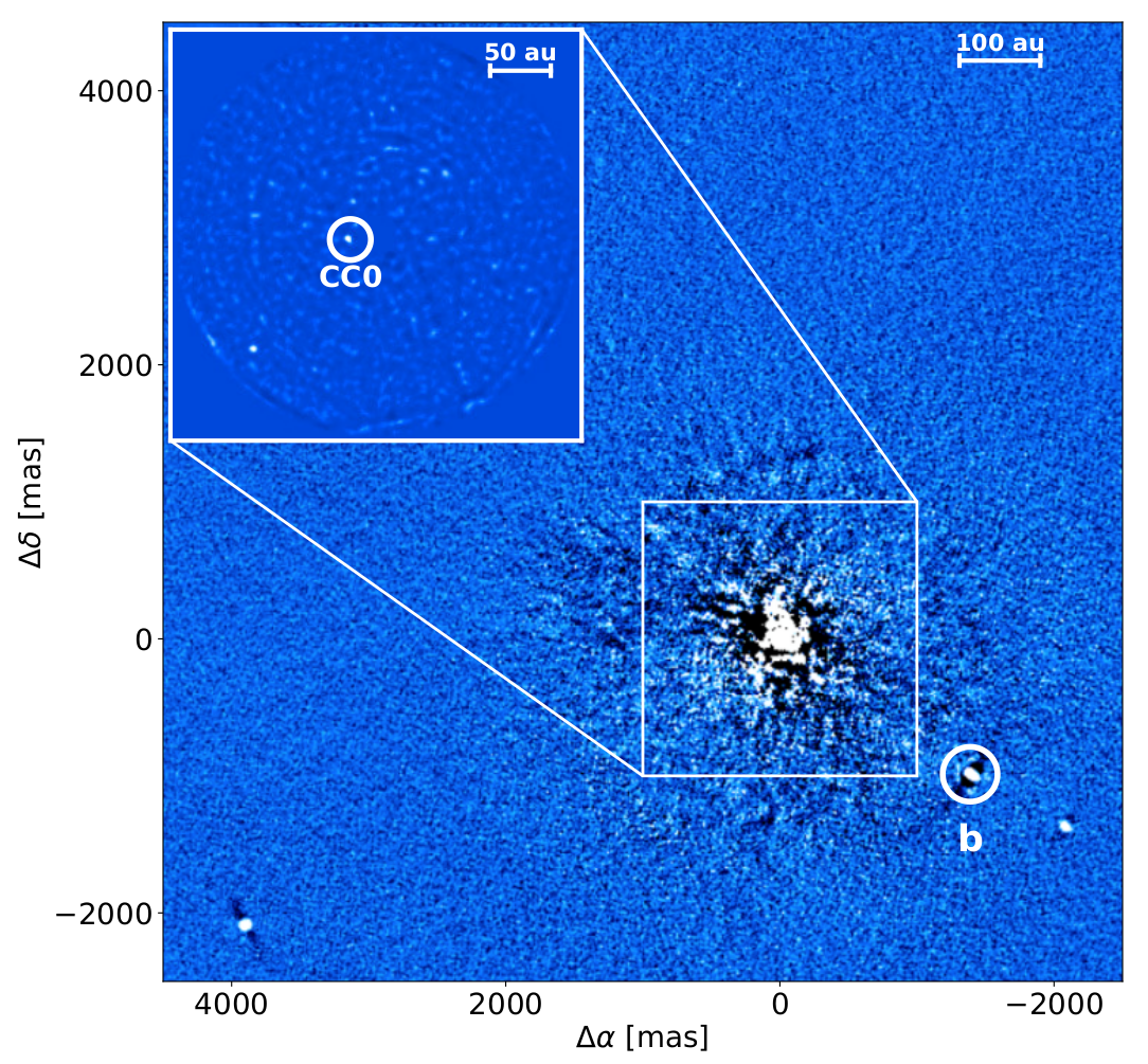
With a sample of 5000 objects at hand, exoplanet demographics is beginning to grasp key aspects of the physical mechanisms lurking beneath the multifaceted hues of the observed exoplanetary architectures. Ascertaining the dependence of planetary properties on stellar mass, and whether their very formation is possible even within the short-lived protoplanetary disks surrounding massive stars, compulsorily requires a complete and unbiased census of the exoplanet population. However, most exoplanet surveys have so far focused on stars not larger than the Sun, and 90% of known exoplanets are closer to their star than the Earth is to the Sun. This strong observational bias, connected to the preference of transits and radial velocities for close-in planets and low-mass stars, has recently started being alleviated by direct imaging, a technique that is instead preferentially sensitive to young giant planets in wide orbits. Radial velocity studies have found that the occurrence of giant planets is higher around more massive stars up to about 2 M_sun; an abrupt turnover is then observed, with the occurrence eventually falling to zero at M>3 M_sun. To clarify if this trend is real, or if a wide-orbit population of giant planets is escaping detection, we have started the B-star exoplanet abundance study (BEAST), a direct-imaging study based on the high-contrast capabilities of SPHERE@VLT. BEAST is looking for exoplanets around 85 B stars belonging to the young (5-30 Myr) Scorpius-Centaurus association. While the survey is still in progress, its early results -that I will show here- are already intriguing: even binary systems such as b Centauri (Janson et al. 2021), or stars doomed to explode as supernovae such as μ2 Scorpii (Squicciarini et al. 2022), can possess their planetary systems, challenging the predictions of conventional formation models.
How to cite: Squicciarini, V.: The B-star exoplanet abundance study (BEAST): at the frontier of planet formation, Europlanet Science Congress 2022, Granada, Spain, 18–23 Sep 2022, EPSC2022-158, https://doi.org/10.5194/epsc2022-158, 2022.
A central question in exoplanetary research is the characterisation of the composition and internal structure of exoplanets. However, the observable parameters of an exoplanet are scarce and generally limited to the planet’s mass and radius and the properties of its host star. This means that it is not possible to fully constrain the internal structure parameters of an exoplanet, such as the iron core mass fraction, the presence of a water layer or the amount of gas, from these observations: The problem is intrinsically degenerate [1,2].
To overcome this difficulty, a Bayesian inference scheme is used, which is an inverse method based on Bayes’ theorem. It updates the previously assumed probability of the internal structure parameters (the prior) based on the probability of the observation given the same parameters (the likelihood), returning the posterior distribution of these parameters.
In our case, the likelihood is determined based on an internal structure model, which calculates the radius of a planet with a given mass and composition based on the planetary structure equations as described in [6]. This calculated radius and the transit depth it implies are then compared to the observed transit depth of the real planet. For the internal structure model, we use the BICEPS code as described in [4] and based on [2,3] to model the core, mantle and water layers of the planet; the atmosphere is modelled separately according to [5]. For the composition, we assume that the planetary composition matches the one of the star exactly [7].
We developed a full grid approach that has multiple advantages over the traditionally used scheme based on Markov chain Monte Carlo methods. To compensate for the higher number of sampling points that such a brute force approach requires, we trained a deep neural network to replace the internal structure model, which significantly reduces the computation time of the model. Additionally, we take into account that the measured masses and radii of the planets in the same system are correlated, since they were measured relative to the same star. This allows for an increase in computation time that is only linear when adding an additional planet. The full approach including the internal structure model is described in more detail in [8].
This method has already been used to characterise the internal structure of various exoplanets observed by the CHEOPS mission, e.g. [8] and [9] (and more submitted). As an example, Figures 1 – 4 show the internal structure of TOI-561 b, c, d and e, calculated using the planetary and stellar parameters published in [9]. Note that the corresponding figures in [9] showing the posteriors of the internal structure parameters unfortunately do not use the published stellar parameters, see [10] for more details.
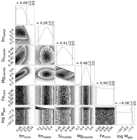
Figure 1. Posterior distribution of the most important internal structure parameters of TOI-561 b using the planetary and stellar parameters published in [9]. The shown parameters are the core and water mass fractions of the solid planet, the molar fractions of Si and Mg in the mantle and Fe in the core and the gas mass of the planet in Earth masses in a logarithmic scale. The dashed lines show the 5 and 95% quantiles, while in the titles the median and the 5 and 95% quantiles are shown.
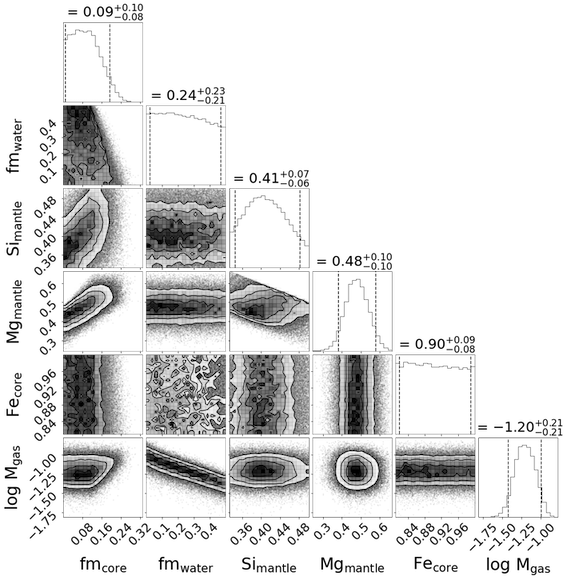
Figure 2. Same as Figure 1 but for planet TOI-561 c.
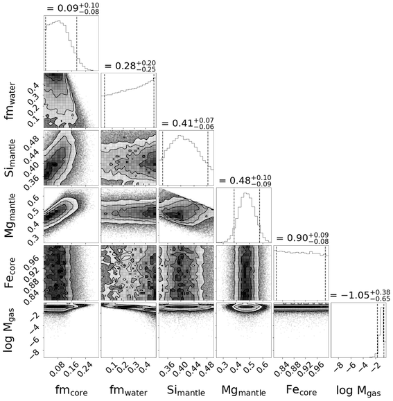
Figure 3. Same as Figure 1 but for planet TOI-561 d.
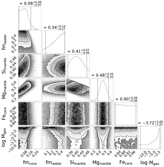
Figure 4. Same as Figure 1 but for planet TOI-561 e.
References:
[1] Rogers, L. & Seager, S. 2010, The Astrophysical Journal, 712, 974
[2] Dorn, C., Khan, A., Heng, K., et al. 2015, A&A, 577, A83
[3] Dorn, C., Venturini, J., Khan, A., et al. 2017b, A&A, 597, A37
[4] Haldemann, J., et al. (in prep.)
[5] Lopez, E. D. & Fortney, J. J. 2014, ApJ, 792, 1
[6] Kippenhahn, R., Weigert, A. & Weiss, A. 2012, Stellar Structure and Evolution, 2nd edn., Astronomy and Astrophysics Library (Berlin Heidelberg: SpringerVerlag)
[7] Thiabaud, A., Marboeuf, U., Alibert, Y., Leya, I., & Mezger, K. 2015, A&A, 580, A30
[8] Leleu, A., Alibert, Y., Hara, N.C., et al. 2021, A&A, 649, A26
[9] Lacedelli, G., Wilson, T.G., Malavolta, L., et al. 2022, MNRAS, 511, 4551–4571
[10] Piotto, G., et al. (in prep.)
How to cite: Egger, J. A., Alibert, Y., Haldemann, J., and Venturini, J.: A Neural Network Based Approach to Modelling the Internal Structure of Transiting Exoplanets and Its Application to Planets Observed by the CHEOPS Mission, Europlanet Science Congress 2022, Granada, Spain, 18–23 Sep 2022, EPSC2022-320, https://doi.org/10.5194/epsc2022-320, 2022.
Warm Jupiters provide a unique opportunity to better understand the formation and evolution of planetary systems. Their atmospheric properties remain largely unaltered by the impact of the host star, and their orbital arrangement reflects a different, and less extreme, migrational history compared to close-in objects. Warm Jupiters are known to cover a wide range of eccentricities but it is unclear which are the dominant formation pathways to explain this observation. Increasing the sample of long-period exoplanets with known radii is thus crucial. In this talk, I report the results of a survey set out to find transiting giants with orbital periods between 20 and 200 days. We selected 50 stars which show a single transit in one TESS sector (27 day baseline) and followed them with ground-based photometric and radial velocity facilities (e.g. NGTS, HARPS). After one year of observations, we report the detection and characterization of ten new transiting warm Jupiters, increasing by 50% the number of known warm Jupiters with precise masses and radii. We infer the metal enrichment of the newly discovered warm Jupiters and explore their influence on the mass-metallicity correlation of giant planets. The growing sample of warm Jupiters allows us to interpret these systems in terms of planet formation models. Finally, these targets orbit bright stars and thus are ideal for follow-up studies of the planetary atmosphere and the system' spin-orbit alignment. This work is a stepping stone for PLATO, as identification and follow up of single transit events will be key in order to detect transiting Earth-sized planets in the habitable zone of Sun-like stars.
How to cite: Ulmer-Moll, S., Lendl, M., Gill, S., Villanueva, S., Hobson, M., Mordasini, C., and Bouchy, F.: From TESS single transits to well-characterized warm Jupiters, Europlanet Science Congress 2022, Granada, Spain, 18–23 Sep 2022, EPSC2022-403, https://doi.org/10.5194/epsc2022-403, 2022.
Detecting exoplanets via the transit method is inherently biased towards short-period planets. Due to the nature of its observing strategy, the Transiting Exoplanet Survey Satellite (TESS) is particularly susceptible to this detection bias; only 12% of planets confirmed by TESS have orbital periods longer than 20 days. It’s crucial that we expand this sample of long-period planets to gain a more complete view of the exoplanet population. One way to do this is using duotransits - planet candidates with two observed transits separated by a large gap, typically two years. The true period of the duotransit is unknown, instead they have a discrete set of possible period aliases. We use these aliases to perform targeted follow-up of the duotransit with the CHaracterising ExOPlanets Satellite (CHEOPS), to recover the true period and ultimately confirm the planet. This allows us to find longer-period planets than are typically found by the TESS mission alone. To select the optimal targets for our CHEOPS follow-up we have developed a specialised pipeline that searches for duotransits in the TESS data. We will present this duotransit pipeline and the results from our CHEOPS follow-up program so far. We have discovered 10 long-period exoplanets, including two planets in the TOI-2076 system, all of which have P > 21 days, RP < 5 REarth and Gaia magnitude < 12. Previously there were only 8 exoplanets discovered by TESS in this exciting parameter space, so our work has more than doubled the sample. These small, long-period transiting exoplanets are amenable to radial velocity follow-up and future atmospheric characterisation with the recently launched James Webb Space Telescope (JWST).
How to cite: Tuson, A. and the CHEOPS Consortium: A Search for Long-Period Transiting Exoplanets with TESS and CHEOPS, Europlanet Science Congress 2022, Granada, Spain, 18–23 Sep 2022, EPSC2022-499, https://doi.org/10.5194/epsc2022-499, 2022.
In this talk I will present our project that is dedicated to the search for transiting planets around hot subdwarfs (sdOB). These peculiar bodies are evolved stars that lost most of their envelope at the tip of the Red-Giant-Branch (RGB). They are small, hot and short-lived stars which have the interesting particularity to have no confirmed planets around them. In this project we perform a wide analysis of all the sdOB observed by the missions Kepler, K2, TESS and CHEOPS in order to, firstly, find transiting planets and compute their occurrence rates and secondly, bring observational constraints for the survival of close-in planets while their host star goes through the RGB. With our current technological means it is often impossible to reach Earth-sized bodies around post-RGB stars, but thanks to the small size of sdOB stars, we are able to do it here. Moreover, the short lifetime of sdOB would most likely not allow for planetary migration or the formation of second-generation planets, which means that short-period planets around them would correspond to planets that were engulfed during the RGB phase. This make them pristine candidates to understand the fate of close-orbiting exoplanets after the RGB phase of their host. In this talk I will present the method we set to analyse the data, from the initial search run to the confirmation steps of interesting signals. I will put an emphasis on the analysis of the 792 sdOB observed during the cycle 1 of the mission TESS as this part is now finished and is the topic of a submitted paper (Thuillier et al. 2022).
How to cite: Thuillier, A., Van Grootel, V., Pozuelos, F., Devora-Pajares, M., Siess, L., and Charpinet, S.: A search for transiting planets around hot subdwarfs - Results from TESS Cycle I, Europlanet Science Congress 2022, Granada, Spain, 18–23 Sep 2022, EPSC2022-514, https://doi.org/10.5194/epsc2022-514, 2022.
In the age of JWST, temperate terrestrial exoplanets transiting nearby late-type M dwarfs provide unique opportunities for characterizing their atmospheres, as well as searching for biosignature gases. In this context, the benchmark TRAPPIST-1 planetary system has garnered the interest of a broad scientific community.
The SPECULOOS (Search for habitable Planets EClipsing ULtra-cOOl Stars) project, an exoplanet transit survey targeting a volume-limited (40 pc) sample of about 1700 late-type (M6 and later) dwarfs using a network of 1m-class robotic telescopes, began its scientific operations three years ago. In this talk, I will present an update on the current status of the survey and an overview of recent results.
In particular, I will describe how an efficient synergy with the TESS mission and other ground-based facilities led to the exciting new discovery of two temperate super-Earths transiting a nearby M6 dwarf, with the outer one orbiting in the habitable zone. In terms of potential for atmospheric characterization, we estimate that this planet is the second-most favorable habitable-zone terrestrial planet found so far after the TRAPPIST-1 planets. The discovery of this remarkable system offers another rare opportunity to study temperate terrestrial planets around our smallest and coolest neighbours.
How to cite: Delrez, L. and the SPECULOOS team: An update on the SPECULOOS project and new results, Europlanet Science Congress 2022, Granada, Spain, 18–23 Sep 2022, EPSC2022-529, https://doi.org/10.5194/epsc2022-529, 2022.
The successful Kepler and TESS missions have discovered thousands of exoplanets and let the community focus on the characterisation of these bodies. One area of research utilises ultra-high-precision photometric and spectroscopic follow-up observations in order to accurately constrain the bulk densities of terrestrial exoplanets. Combining these observables with Bayesian internal structure modelling that uses geological equations of state, we can start to learn about the compositions of planets around main-sequence stars for the first time. Importantly, by studying multi-planet systems we can conduct comparative planetology that can reveal important aspects that challenge our knowledge of planet formation and evolution via the contrastment of the observational and modelling results of a planet against its neighbours.
In this talk, I will present observational studies characterising multi-planet systems initially discovered with TESS and followed-up with ultra-high precision photometry from the recently launched CHEOPS satellite and ground-based RV instruments, such as HARPS and HARPS-N. Additionally, I will discuss our Bayesian internal structure and atmospheric escape analyses, and present the results of utilising such models on several key, multi-planet systems observed with CHEOPS, such as TOI-1064 and TOI-561, that are expected to become cornerstones of exoplanet characterisation due to the questions they raise about planet formation, the system multiplicity, or the amenability to atmospheric observations. Important knowledge about these new systems was uncovered via the refined radii, masses, and densities, a combination of precise observations using a new generation of instruments across different techniques, and cutting-edge planetary internal structure modelling. Therefore, utilising these resources we are at the beginning of a new era in characterising terrestrial bodies outside of our Solar System that will be strengthened with JWST.
How to cite: Wilson, T.: Characterising the internal structures of small exoplanets with CHEOPS, Europlanet Science Congress 2022, Granada, Spain, 18–23 Sep 2022, EPSC2022-944, https://doi.org/10.5194/epsc2022-944, 2022.
In this porter, we present SHERLOCK, an end-to-end pipeline that allows the users to explore the data from space-based missions such as TESS and Kepler/K2 to search for planetary candidates. It can be used to recover alerted candidates by the automatic pipelines such as the Science Processing Operations Center (SPOC) and the Quick Look Pipeline (QLP), the so-called Kepler objects of interest (KOIs) and TESS objects of interest (TOIs), and to search for candidates that remain unnoticed due to detection thresholds, lack of data exploration or poor photometric quality. To this end, SHERLOCK has six different modules to (1) acquire and prepare the light curves from their repositories, (2) search for planetary candidates, (3) vet the interesting signals, (4) perform a statistical validation, (5) model the signals to refine their ephemerides, and (6) compute the observational windows from ground-based observatories to trigger a follow-up campaign. To execute all these modules, the user only needs to fill in an initial yaml file with some basic information, such as the star ID, the cadence to be used, etc., and use sequentially a few lines of code to pass from one step to the next. Alternatively, the user may provide SHERLOCK with the light curve in a csv file, where the time, the normalized flux, and the flux error need to be given in columns comma-separated format. SHERLOCK is being used in the SPECULOOS project, which is searching for transiting Earth-sized planet orbiting ultra-cool stars in the habitable zone. These planets provide the best opportunities for future atmospheric characterization of temperate small rocky worlds. In addition, SHERLOCK is used in the FATE project, a survey that aims to find transiting planets orbiting hot subdwarfs. Thanks to their small sizes, these stars represent excellent opportunities for addressing the question of the evolution of planetary systems once their host stars left the main sequence and passed through the red giant branch phase. SHERLOCK is an open-source friendly-user package available at https://github.com/franpoz/SHERLOCK
How to cite: Pozuelos, F. J., Dévora-Pajares, M., Thuillier, A., Van Grootel, V., and Suarez Yanes, J. C.: SHERLOCK: A python pipeline to explore space-based observations in the search for planets, Europlanet Science Congress 2022, Granada, Spain, 18–23 Sep 2022, EPSC2022-970, https://doi.org/10.5194/epsc2022-970, 2022.
Planet-star interactions are considered to have a Janus-faced character. Most of the known forms belong to star-to-planet interactions, for which well-known examples are the stellar irradiation, rotation and stellar activity affecting the planet. We can only rarely see planet-to-star scenarios, mostly because of the smaller planets can less affect the stellar physics. In this talk, we review three examples for such scenarios, including commensurabilities between the stellar spin and the planetary orbit, excitation of stellar activity, and stellar oscillations suffering planetary perturbations. The observational basis of our examples, Kepler-13A, AU Mic and WASP-33 also cover the three major exoplanet missions: Kepler, CHEOPS and TESS, nicely showing how the space-based exoplanet photometry started revealing the (almost) hidden face of Janus.
How to cite: Szabó, G.: Examples for planet-to-star interactions, Europlanet Science Congress 2022, Granada, Spain, 18–23 Sep 2022, EPSC2022-1059, https://doi.org/10.5194/epsc2022-1059, 2022.
The orbits and dynamics of exoplanet systems can unveil their tales of formation, migration, star-planet interactions, and atmospheric properties. Kepler, TESS, and soon PLATO deliver an unprecedented wealth of new photometric data on this matter, while ground-based follow-up and radial velocity instruments add valuable insights. Here, I will present how we can unite and untangle all this data on exoplanets' orbits and dynamics using allesfitter. This open-source python software enables flexible and robust inference of stars and exoplanets from photometric and radial velocity data. Allesfitter offers a rich selection of orbital and transit/eclipse models, accommodating multiple exoplanets, multi-star systems, transit-timing variations, and phase curves. It can also help mitigate and/or study stellar variability, starspots, and stellar flares. I will highlight some of allesfitter's science output on examples of exoplanet dynamics (e.g., TOI-270 and TOI-216) and orbital phase curves (e.g., WASP-18 and WASP-121). With TESS' extended mission and PLATO on the horizon, a wealth of new data soon face us, allowing TTV and phase curve studies of dozens of such systems over many years.
How to cite: Günther, M. N.: Studying exoplanet orbits & dynamics with allesfitter, Europlanet Science Congress 2022, Granada, Spain, 18–23 Sep 2022, EPSC2022-1180, https://doi.org/10.5194/epsc2022-1180, 2022.
The composition of several exoplanet atmospheres has been largely debated with contrasting results in the literature. Low- and high-resolution spectroscopy offer complementary views, although sometimes appear to be in sparkling contrast. We present a new approach to simultaneously model low- and high-resolution observation and apply this method to resolve known controversies in the literature. We show that the synergy between different techniques of observations is significantly more informative than the separate analyses. We recommend the joint analysis of low- and high-resolution exoplanet spectra to fully exploit the potential of upcoming space missions, such as JWST, Twinkle and Ariel.
How to cite: Morello, G., Pallé, E., Orell-Miquel, J., Masseron, T., and Esparza-Borges, E.: Synergies between low- and high-resolution spectroscopy of exoplanet atmospheres, Europlanet Science Congress 2022, Granada, Spain, 18–23 Sep 2022, EPSC2022-1233, https://doi.org/10.5194/epsc2022-1233, 2022.
EXOA15 | Habitability and biosignatures for the search for life in our Solar system
Introduction
One of the main topics of astrobiology research is the study of life’s limits in stressful environments. The study of organisms in extreme environments might give an indication about their potential adaptive plasticity, in the view of a climate change perspective, the terrestrial geological past and future scenarios, as well as extra-terrestrial habitats such as Mars’ surface. Lichens - with their excellent adaptive abilities - represents an extremely interesting case study. Several astrobiological studies involving lichens - that are symbiotic association between a fungus and an alga and/or acyanobacterium - proved the ability of these organisms to resist and thrive in extreme environments such as space and Mars’ surface simulated conditions [1, 2]. We have already tested the lichen species Xanthoria parietina (L.) Th. Fr. in simulated space conditions, that was able to survive and to reactivate after exposure [3]. X. parietina is a cosmopolitan foliose lichen that grows on barks and rocks [4]. This species shows high tolerance to air pollutants, heavy metals, and resistance to UV-radiation thanks to the shielding properties of the secondary metabolite parietin [5, 6]. Here we present a new study on the survival of X. parietina under simulated Mars conditions performed at the Mars Simulation Facility of the DLR Institute of Planetary Research in Berlin (Fig.1).
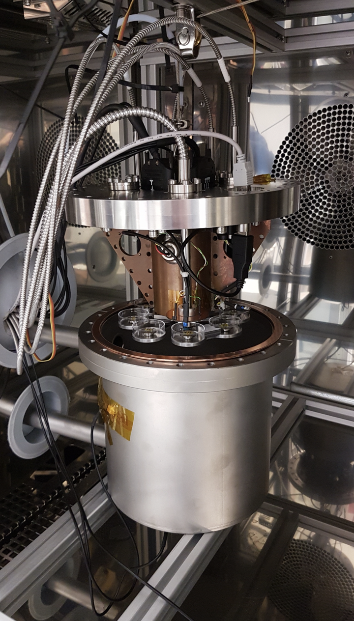
Figure 1 - Mars Simulation Facility at DLR with the opened experiment chamber.
Methods
The aim of the study was to assess the survivability of Xanthoria parietina under simulated Mars conditions for 30 days [7, 8]. Inside the Mars simulation chamber, eight samples (Fig.2) were exposed to the simulated atmospheric conditions of Mars of which four were fully UV-irradiated with day-night cycles (FM, Full-Mars) and the other four kept in darkness (DM, Dark-Mars). A three-gas mixture of 95% CO2, 4% N2 and 1% O2 was used as best approximation of Mars-like atmospheric conditions, with a constant pressure of 600Pa. Temperature and humidity were subjected to day-night cycles, reaching during daytime 15°C and 0% RH, and during night -55°C and 100% RH (Fig.3) according to Martian thermophysical conditions at mid-latitudes. UV-radiation for FM samples was simulated using a Xenon UV-lamp (spectral range 200 nm – 2200 nm) that was automatically turned on for 16 h (day) and turned off for 8 h (night) daily. The total average radiation dose for FM was 2452.32 J/cm2 and the average instantaneous irradiance on the sample spots was 14,2 W/m2 [9]. Four other samples (Fig.2) were kept in control conditions during the experiment, at the constant temperature of 25°C, daily wetted and 12h dark and 12h light (ca. 50 μmol m-2 s-1 PAR photons). Several analyses were carried out to study all the samples before, during and after the exposure to the extreme Mars conditions. In detail, this experiment was performed aiming:
- to monitor the lichen vitality through chlorophyll a fluorescence (FV/FM) as photosynthetic efficiency parameter, carrying out in situ and after treatment analyses,
- to evaluate the oxidative stress due to the extreme conditions, highlighting eventual changes in the lichen carotenoids’ Raman signatures,
- to verify eventual modifications in the infrared features (peak shifting) in the lichen FTIR reflectance spectrum possibly related to UV-photodegradation effects,
- to highlight possible variations in the lichen ultrastructure through TEM analysis.
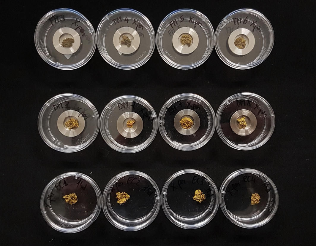
Figure 2 - Xanthoria parietina samples ready for the experiment. First row (from above): full Mars samples, second row: dark Mars samples, third row: control samples.
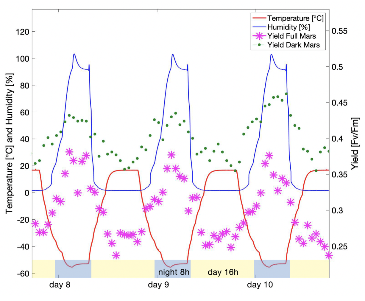
Figure 3 - Detail of the day-night cycles of the simulated Mars conditions (temperature, red thick line; humidity, blue thin line) and fluorescence variation values for both the treatments (FM and DM).
Results
The results showed significant differences between FM and DM photosynthetic efficiency parameter during exposure to Mars environment, exhibiting FV/FM values correlated with temperature and humidity day-night cycles (Fig.3). The FV/FM recovery values showed significant differences between the treatments too, highlighting that FM conditions caused stronger effects on fluorescence values. Additional analyses show possible changes in the Raman and FTIR spectra of the irradiated samples with several features involved. Overall, Xanthoria parietina was able to survive to FM conditions, and for this reason it may be considered a candidate for long exposure in space and evaluations on the photodegradability of parietin in extreme conditions.
Reference
[1] Onofri, S., de la Torre, R., de Vera, J. P., Ott, S., Zucconi, L., Selbmann, L., Scalzi, G., Venkateswaran, K. J., Rabbow, E., Sánchez Iñigo, F. J., and Horneck, G. (2012). Survival of rock-colonizing organisms after 1.5 years in outer space. Astrobiology, 12(5), 508-516.
[2] De Vera, J. P., Möhlmann, D., Butina, F., Lorek, A., Wernecke, R., and Ott, S. (2010). Survival potential and photosynthetic activity of lichens under Mars-like conditions: a laboratory study. Astrobiology, 10(2), 215-227.
[3] Lorenz, C., Bianchi, E., Benesperi, R., Loppi, S., Papini, A., Poggiali, G., & Brucato, J. R. (2022). Survival of Xanthoria parietina in simulated space conditions: vitality assessment and spectroscopic analysis. International Journal of Astrobiology, 1-17.
[4] Nimis P.L., 2016. ITALIC - The Information System on Italian Lichens. Version 5.0. University of Trieste, Dept. of Biology, (http://dryades.units.it/italic), accessed on 2022, 05, 09. for all data contained in the taxon pages, including notes, descriptions, and ecological indicator values.
[5] Silberstein, L., Siegel, B., Siegel, S., Mukhtar, A., and Galun, M. (1996). Comparative Studies on Xanthoria parietina, a Pollution Resistant Lichen, and Ramalina duriaei, a Sensitive Species. I. Effects of Air Pollution on Physiological Processes. The Lichenologist, 28:355-365.
[6] Solhaug, K. A., and Gauslaa, Y. (1996). Parietin, a photoprotective secondary product of the lichen Xanthoria parietina. Oecologia, 108:412-418.
[7] Lorek, A., and Koncz, A. (2013). Simulation and measurement of extraterrestrial conditions for experiments on habitability with respect to Mars. In Habitability of Other Planets and Satellites (pp. 145-162). Springer, Dordrecht.
[8] De Vera, J. P., Schulze-Makuch, D., Khan, A., Lorek, A., Koncz, A., Möhlmann, D., and Spohn, T. (2014). Adaptation of an Antarctic lichen to Martian niche conditions can occur within 34 days. Planetary and Space Science, 98, 182-190.
[9] Cockell, C. S., Catling, D. C., Davis, W. L., Snook, K., Kepner, R. L., Lee, P., and McKay, C. P. (2000). The ultraviolet environment of Mars: biological implications past, present, and future. Icarus, 146(2), 343-359.
How to cite: Lorenz, C., Bianchi, E., Poggiali, G., Alemanno, G., Benesperi, R., Brucato, J. R., Garland, S., Helbert, J., Lorek, A., Maturilli, A., Papini, A., de Vera, J.-P., and Baqué, M.: Survivability of Xanthoria parietina in simulated Mars conditions for 30 days, Europlanet Science Congress 2022, Granada, Spain, 18–23 Sep 2022, EPSC2022-189, https://doi.org/10.5194/epsc2022-189, 2022.
Some organisms have shown to be able to naturally survive environments which we consider extreme, including the Low Earth Orbit, or even Outer Space. These microorganisms have natural mechanisms to repair severe DNA damage, such as the caused by ionizing and non-ionizing radiation or extreme temperatures and pressures. Some examples are Deinococcus radiodurans, which proved to be capable of surviving in the Exposure Facility of the International Space Station (ISS) for up to three years, and tardigrade species, such as Ramazzottius varieornatus, which are some of the most resilient known organisms. In this study, performed at the Barcelona Biomedical Research Park in collaboration with Hospital del Mar, survival under simulated Low Earth Orbit environmental conditions was tested in engineered and wild-type Escherichia coli strains. Ionizing radiation resistance was enhanced by transforming the Dsup gene from R. varieornatus and two genes from D. radiodurans involved in DNA damage repair, RecA and uvrD. This enhancement, together with a directed evolution process, resulted in a significant increase in the surviving fraction of the E. coli strain protected with the Dsup gene after a high dose, up to 3000 Gy, of ionizing radiation exposure in the form of a continuous spectrum of X-ray photons. Additionally, the survival to wide ranges of temperatures and low pressures was tested for the same strains, revealing a lack of relevance of cell aggregation for survival under the mentioned conditions in contrast with the case of D. radiodurans. However, survival rates showed no enhancement for any of the new E. coli strains. In a new collaboration with the Subterranean Laboratory of Canfranc, both the absence of radiation and extreme levels of radiation will be further studied. Additionally, an extreme environments analogue for several environmental conditions will be built, allowing for more specific testing on a controlled environment. This research represents a first step in the creation of new bacterial strains engineered to survive severe conditions and adapting existing species for their survival in remote environments, like extra-terrestrial habitats. These species could pave the road for future human expeditions, helping develop environments hospitable to life. In addition, studying the efficacy and the functioning of the genetic mechanisms used in this study could be beneficial for fields such as ecological restoration and medical and life sciences engineering, addressing treatments and/or diseases caused or related to radiation and DNA damage. Space is believed to be the last frontier, but the truth is, we are still a frontier to ourselves.
How to cite: Puig, J., Knödlseder, N., Quera, J., Algara, M., and Güell, M.: DNA Damage Protection for Enhanced Bacterial Survival Under Simulated Low Earth Orbit Environmental Conditions in Escherichia coli, Europlanet Science Congress 2022, Granada, Spain, 18–23 Sep 2022, EPSC2022-378, https://doi.org/10.5194/epsc2022-378, 2022.
Martian regolithic soil is considered an inhospitable environment to life as we know it with low availability of nutrients and the presence of powerful oxidants, namely perchlorate salts. Extreme microorganisms such as cyanobacteria of the genus Chroococcidiopsis dominate rock-dwelling communities in extreme deserts resembling the actual Martian environment. The strain Chroococcidiopsis 029, extremely tolerant to desiccation, ionizing, and UV radiation, can thrive in Mars-like conditions in a dried state. In the present work, we investigated the response of Chroococcidiopsis 029 when grown for a 3-week period using Martian regolith simulant containing 2.4 mM perchlorate anions. The growth either in the planktonic cells or biofilm life style was monitored following the in chlorophyll a content. The cellular and molecular responses to 2.4 mM perchlorate anions was studied following cell viability according to: i) PCR-PMA assay, ii) changes in gene expression of three SOD-coding genes (soda 2.1, soda.2, and sodC), and iii) production of intracellular ROS as revealed by CLSM. Results suggested that perchlorate did not compromise cell viability and that a significant over-expression of three SOD isoforms occurred after the one-week exposure with a greater expression of the membrane-bound MnSOD (sodA 2.1) in comparison to the cytoplasmic isoforms MnSOD (sodA 2.2) and Cu/ZnSOD (sodC). The accumulation of ROS within the cells was observed after 1-day exposure to perchlorate. Future investigations on the effect of Mars-like conditions in hydrated biofilms with 2.4 mM ClO4- and Martian regolith simulant will be carried out supported by the Europlanet scholarship 2024. These results are relevant for the habitability of Mars and the development of In-situ Resource Utilization.
How to cite: Gallego Fernandez, B., Mosca, C., Fagliarone, C., and Billi, D.: Responses of a desert cyanobacterium to prolonged exposure to perchlorate: implications for the habitability of Mars and In-Situ Resource Utilization, Europlanet Science Congress 2022, Granada, Spain, 18–23 Sep 2022, EPSC2022-537, https://doi.org/10.5194/epsc2022-537, 2022.
Introduction. The harsh oxidative and radiative conditions of the Martian environment influence the fate of organic molecules present on its surface. Formation of radical species was suggested to transform organic macromolecules into carboxylic acid through Fenton chemistry (1, 2) or irradiation semiconductor surfaces (3). Aromatic carboxylic acids such as phthalic acid or benzoic acid are thought to be abundant on the Martian surface as they are in stable intermediate oxidation states and can be formed from the oxidation of Polycyclic Aromatic Hydrocarbons (PAHs) (1, 4) or alkylbenzene compounds (4) coming from endogenous or exogenous sources. Because benzene carboxylates are metastable, they should not be entirely oxidized into volatile molecules such as CO2 or O2, but instead, ionized by solar radiation to form organic salts (2, 4, 5). Benner et al. (2000) suggested that the low volatility of these salts could compromise their in situ detection through thermal extraction analyses as performed by analytic chemistry laboratories onboard Martian surface probes, such as the Sample Analyzer at Mars (SAM) experiment onboard Curiosity rover or the Mars Organic Molecular Analyzer (MOMA) instrument of the Rosalind Franklin Exomars rover (4-6). To determine the possibility to identify these molecules through direct or indirect detection on Mars, we examined laboratory results from SAM and MOMA-like Gas Chromatography-Mass Spectrometry (GC-MS) analyses of two acid/salt couples (phthalic acid/calcium phthalate and benzoic acid/calcium benzoate). We analyzed the difference in behavior and signatures of both molecular forms when using pyrolysis and wet chemistry experiments used in SAM and MOMA, and the relevance of these results in the search of organic molecules on Mars.
Method. Synthetic samples were made by mixing the carboxylic acid molecules or their organic salts standards at 1wt.% in fused silica, to simulate a relatively inert mineral matrix. The samples were pyrolyzed in SAM-like conditions with a ramp of 35°C.min-1 and in MOMA-like conditions in flash pyrolysis at 500°C and 800°C. The volatiles released from each sample were analyzed by Evolved Gas Analysis (EGA) and Gas Chromatography-Mass Spectrometry (GC-MS). We also performed derivatization experiments to help detect refractory organic compounds, with N,N-methyl-tert-butyl-dimethylsilyltrifluoroacetamide (MTBSTFA), used for wet chemistry experiments in SAM, and N,N-Dimethylformamide dimethyl acetal (DMF-DMA), to be used in the MOMA experiment of the ExoMars mission.
Organic acid/salt behavior under pyrolysis conditions. As predicted by Benner et al. (4), when analyzed through pyrolysis-GC-MS, the organic salts species did not produce the organic parent molecule (phthalic acid or benzoic acid (Fig. 1 (a)). However, we have identified two by-products characteristic of the degradation of the organic salts, diphenylmethane (Fig. 1 (b)) and triphenylmethane (Fig.1 (b)) which were absent of the chromatograms of the acid species. These results show that for both carboxylic acid couples studied, the acid and the salt don’t follow the same degradation pathway resulting in differences in the species detected as well as major differences in the abundance of products observed in the chromatograms. This means that if carboxylic acids are present on Mars in their saline form linked to calcium cations, we would not be able to identify it through the detection of its acid form with the SAM nor MOMA pyrolysis set-ups, but rather through the detection of characteristic by-products that would serve as indirect clues for identification.
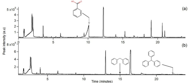
Figure 1. Chromatograms obtained under the same analytical conditions as the pyrolysis in SAM. (a) benzoic acid mixed at 1 wt. % in fused silica and (b) calcium benzoate mixed at 1 wt. % in fused silica.
Organic acid/salt derivatized with MTBSTFA and DMFDMA.

Figure 2. Bar chart representing the abundance of derivatized benzoic acid obtained with calcium benzoate and benzoic acid. The derivatization reagent used was DMFDMA (a) and MTBSTFA (b).
When derivatized with DMFDMA or MTBSTFA, both the acid and the organic salt produced the derivatized product of the carboxylic acid. Both the phthalic acid and benzoic acids have a higher derivatization yield than their salt counterpart with both derivatization reagents. This is likely due to a better availability of the hydrogen on the carboxylic acid function. Moreover, we obtained a higher yield of both the acid and the salt with MTBSTFA than with DMF-DMA, with the loss of detection of calcium phthalate derivative with the latter. In conclusion, if present in the Martian soil, aromatic organic salts could be directly detected through wet chemistry experiments, showing the complementarity of this technique with pyrolysis.
References. (1) Oró et al. (1979) Life Sciences and Space Research, 77-86. (2) Donald et al. (2013) Science. (3) Fox et al. (2019) Journal of Geophysical Research: Planets 124, 3257-3266. (4) Benner et al. (2000) Proceedings of the National Academy of Sciences 97, 2425-2430. (5) Lasne et al. (2016) Astrobiology 16, 977-996. (6) Hakkinen et al. (2014) Environ Sci Technol 48, 13718-13726.
How to cite: Mcintosh, O., Szopa, C., Freissinet, C., Buch, A., and Boulesteix, D.: Analysis of aromatic organic salts with gas chromatography-mass spectrometry and implications for their detection at Mars surface with in situ experiments , Europlanet Science Congress 2022, Granada, Spain, 18–23 Sep 2022, EPSC2022-590, https://doi.org/10.5194/epsc2022-590, 2022.
Energy from active serpentinization processes potentially fuelled the origin of life on Earth, thus, if serpentinite-impacted sites facilitate microbial habitability, it is important to understand the source and retention of biological signatures in serpentine rocks. Investigating biological signatures in terrestrial analogues of serpentinite-impacted environments is also essential for interpreting molecular signature preservation on extra-terrestrial bodies.
To expand knowledge on the types of biological signatures directly derived from living microorganisms (intact polar lipids, IPLs), and both living and dead microorganisms (core lipids), mass spectrometry analysis was performed on Chimaera serpentinite rocks from Antalya Province, Turkey. Brucite rocks were dominated by IPLs from fungal, eukaryotic origin but in contrast, travertine samples had IPL profiles consistent with a mixed fungal, archaeal and bacterial community. The abundance and diversity of archaeal IPLs was significantly higher in the travertine compared to the brucite, and the abundance of archaeal IPLs inside the travertine rock was highest. Archaeal specific core lipids identified inside the brucite rock were not observed as IPL counterparts, suggesting the presence of a non-viable or fossil archaeal community. Comparing IPL profiles with core lipids can discriminate between living microbial communities, necromass, and fossils to combine as a promising molecular tool for identification and interpretation of bio-signatures in serpentinite-impacted sites. Continuing survey of serpentinization samples on Earth can act as analogue environments and provide valuable insight into microbial habitability on Mars and other planetary objects.
How to cite: Zetterlind, A., Rattray, J. E., Smittenberg, R. H., Potiszil, C., ten Kate, I. L., and Neubeck, A.: Lipidomics Based Microbial Ecology Snapshot of Ophiolitic Rocks, Europlanet Science Congress 2022, Granada, Spain, 18–23 Sep 2022, EPSC2022-952, https://doi.org/10.5194/epsc2022-952, 2022.
ODAA1 | Europlanet for Emerging Space Countries
From March 16th to 26th 2022, for the first time in Togo, we organized an astronomy outreach event: “Togo under the stars”. This event is the result of a collaboration between the French association SpaceBus France and the Togolese association SG2D (Science Géologique pour un Développement Durable).
During two weeks, four French astronomers and six Togolese geologists traveled the country to reach a wide public. We visited schools, villages, and public squares and gave astronomy workshops in six cities: Kara, Sokodé, Atakpamé, Kpalimé, Aného and Lomé.
At each occasion, we proposed activities created by SpaceBus France, designed to be fun and interactive. These activities include a presentation of the Solar system using a scaled 3D printed model, a hands-on exercise on meteorites with different kinds of meteorites and terrestrial rocks to recognize them, an introduction to space travel and rocket science using lego models, and observations of both the Sun and the night sky using several telescopes.
In Lomé, we also provided an astronomy training for teachers of all levels, giving them educational tools and teaching resources developed by research institutions such as Europlanet Society, Paris Observatory, CNES, ESA, etc. These free resources and available on the internet can easily used to teach astronomy in classroom.
Togo under the stars has been a great success, reaching over 10.000 Togolese in total, with extremely positive feedback. This project, which was possible thanks to financial support from Europlanet, thus allowed the Togolese to have their first major astronomy outreach event. It offered a unique opportunity for the students to meet and exchange with astrophysicists and geologists, while the interaction with teachers insured a long-lasting impact on future generations.
More information : https://www.spacebusfrance.fr/le-togo-sous-les-etoiles
How to cite: de Assis Peralta, R. and Berard, D.: Togo under the stars: a science outreach tour for the Togolese, Europlanet Science Congress 2022, Granada, Spain, 18–23 Sep 2022, EPSC2022-1177, https://doi.org/10.5194/epsc2022-1177, 2022.
Planetary Geology and Astrobiology focused research have significantly grown in the last decades, where the US, European countries and China have been leading the path through NASA, ESA and CNSA space programs. This research has been more limited in South America, sometimes due to the lack of an explicit space program or where this program exists but developed at a smaller scale or focused on different goals. In spite of this, a growing number of scientists has been actively conducting research, directly or indirectly, related to these topics. Here is a brief and clearly biased and non-exhaustive summary shows how diverse this research is, taking some examples in Argentina and other countries such as Chile and Brazil, but being aware that other countries such as Colombia and Mexico also have a growing Planetary Geology and Astrobiology community.
Structural geology, geomorphology and tectonics in our planet is a matter of intense research in Argentina, particularly in the Andean region. Similar studies in other planetary bodies such as Mars, on the other hand, are more limited. In spite of this, it is worth mentioning the research conducted by Dr. Mauro Spagnuolo and colleagues of the IDEAN (Instituto de Estudios Andinos Pablo Groeber, Buenos Aires, Argentina, http://www.idean.gl.fcen.uba.ar/). This group has been actively collaborating and working on topics such as planetary mapping, geomorphology, structural geology and sedimentary processes of Mars and Titan surface.
The question of the possibility of life on other planets brings the need to be able to recognize extinct or extant life, particularly in the sedimentary record. The approach is to study how life develops in a diversity of environments, typically extreme environments, to understand how the signals of life are preserved in the sedimentary record (biosignatures). The study of microbial activity and their biosignatures has been the focus of research of Dr. Fernando Gomez and colleagues (https://fernandojgomez.github.io/FernandoJGomez/team/) from the CICTERRA (Centro de Investigaciones en Ciencias de la Tierra) and Dr. Douglas Galante (https://orcid.org/0000-0002-3265-2527) and Amanda Bendía (https://orcid.org/0000-0003-0042-8990) from the University of São Paulo (Brazil) by using a combination of sedimentolgical, biogeochemical and microbiological tools in order to explore the limits of life and its sedimentary record.
Dr. Pamela Such is a geologist from Argentina, and currently a SETI Institute research affiliate (https://www.seti.org/affiliates/pamela-such) who works mainly in developing the techniques and instrumentation necessary for the exploration of space resources. For example she collaborated with Dr. Pablo Sobron (SETI/NASA; Impossible Sensing Founder), testing LIBS laser and Raman instruments in environments of high UV and altitude and deficient oxygen levels in the Andes and with Dr. Mike Daly, OLA Instrument, OSIRIS-REx mission. She also has recently participated in the simulated mission to Mars, AMADEE 18, in the Oman desert. She has also recently led a project and research to study the feasibility of exposure and survival of Quinoa seeds to extra-planetary conditions to explore the development of crops during missions to the Moon and Mars.
The mineralogy and cosmochemistry of meteorites and its relevance to understand the formation of our Solar System has been the focus of intense research by Maria Eugenia Varela and colleagues of the ICATE (Instituto de Ciencias Astronómicas, de la Tierra y el Espacio) (https://icate.conicet.gov.ar/). In addition Dr. Varela is a member of the Argentinian Research Unit in Astrobiology (http://astrobioargentina.org/argentinian-research-unit-in-astrobiology/) where some scientists also explore the possibility of life in other planetary bodies. Another approach to meteorites and other space bodies has been developed by Dr Daniel Acevedo CADIC (Ushuaia, Argentina) and colleagues, by studying the numerous impact craters in Argentina and South America. For example, it is well known for their research in the Bajada del Cielo impact field in Chubut, southern Argentina. This research has been published in numerous papers and summarized in a really interesting book titled Impact Craters in South America (https://link.springer.com/book/10.1007/978-3-319-13093-4).
Dr. Giovanni Leone is an Italian geophysicist and volcanologist from the Atacama University, Chile (https://www.linkedin.com/in/giovanni-leone-73558185/?originalSubdomain=cl). His research includes Planetary Simulants, using the basaltic rocks from Atacama desert as a Moon and Mars geochemical analogues for testing rovers and carrying on experiments for future planetary settlements; Space Biomining, exploring the role of bacteria in low-water environments for the extraction of useful minerals (i.e. rare earth elements, copper, etc.); and Muography, the use of muons naturally produced by the interactions between galactic cosmic rays and atmosphere, for example, for the imaging of the internal structure of volcanoes. It is also worth mentioning his recent research on Mars surface and interior by combining geophysical and modelling techniques, as well as availability of important resources like water, and the studies about meteorites found in the Atacama Desert by Dr. Millarca Valenzuela (https://www.astrofisicamas.cl/millarca-valenzuela/).
Aside from the purely scientific approach to planetary geology, it worth to mention the activities developed by that SpaceBee Technologies (http://www.spacebeetech.com/), and its diverse team of geologists and engineers from Cuba and Argentina ( http://www.spacebeetech.com/team.html). This includes the development of a low-cost lunar rover named RoverTito, designed to contribute to the exploration of the Moon and to explore its potential for human habitability and for making the space accessible for future generations. Understanding the lunar regolith, the detection of structures such as lava tunnels or the distribution of solid water (ice) by using a set of geophysical techniques is between the goals of the SpaceBee Technologies project.
All these interesting efforts and contributions in planetary geology have been catalyzed by the individual and/or collective interest of some researchers and technology-focused teams, being the driving force of the curiosity for space exploration. Clearly, joining efforts into a more organized and better funded program where different institutions along South America can collaborate would increase the potential and collaborative research of all these researchers and engineers. This calls attention to the need to create the space for this discussion to take place and where people can share these activities and experiences and this may help to set the lines for a future planetary space program in South America.
How to cite: Gomez, F., Leone, G., Losarcos, J. M., and Santillan, F. A.: Planetary Geology and Astrobiology research in South America, Europlanet Science Congress 2022, Granada, Spain, 18–23 Sep 2022, EPSC2022-1246, https://doi.org/10.5194/epsc2022-1246, 2022.
ODAA2 | Diversity and Inclusiveness in Planetary Sciences
The EPEC (Europlanet Early Career) network was launched at EPSC in 2017, and since that day our community has grown exponentially. The idea was to create a friendly environment where early careers could meet, confront the complex dynamics of the academic career, and be involved in activities with the support of the Europlanet Society. In fact, the Europlanet Society itself felt the need of having a space where early-career researchers could gather and grow, and senior scientists played a fundamental role in supporting the new generations.
Today, EPEC reached that goal and is committed to building a strong network among young professionals by nurturing a supportive environment to develop various ideas within each themed working group (WG) and developing leadership skills. The EPEC community is open to all early-career planetary scientists and space professionals who obtained their last degree (e.g. MSc or PhD) less than 7 years ago.
Supervisors (and future supervisors) are of great help to spread the word about our community. By doing this, part of networking and understanding of the field will be complemented by the supervisor's perspective.
EPEC is structurally organized around 7 WGs (Fig.1): Communications, Diversity, EPEC@EPSC, Outreach, Annual Week, Early Career Support, and Future Research. Each WG, usually led by two Co-Chairs, works within its purview to best address the needs of early-career researchers and reflects on actions that can be implemented. This includes interviews, contests, and campaigns, continuously evolving thanks to new members and new ideas. We are working hard for every voice to be heard and this makes EPEC a very diverse and inclusive community.
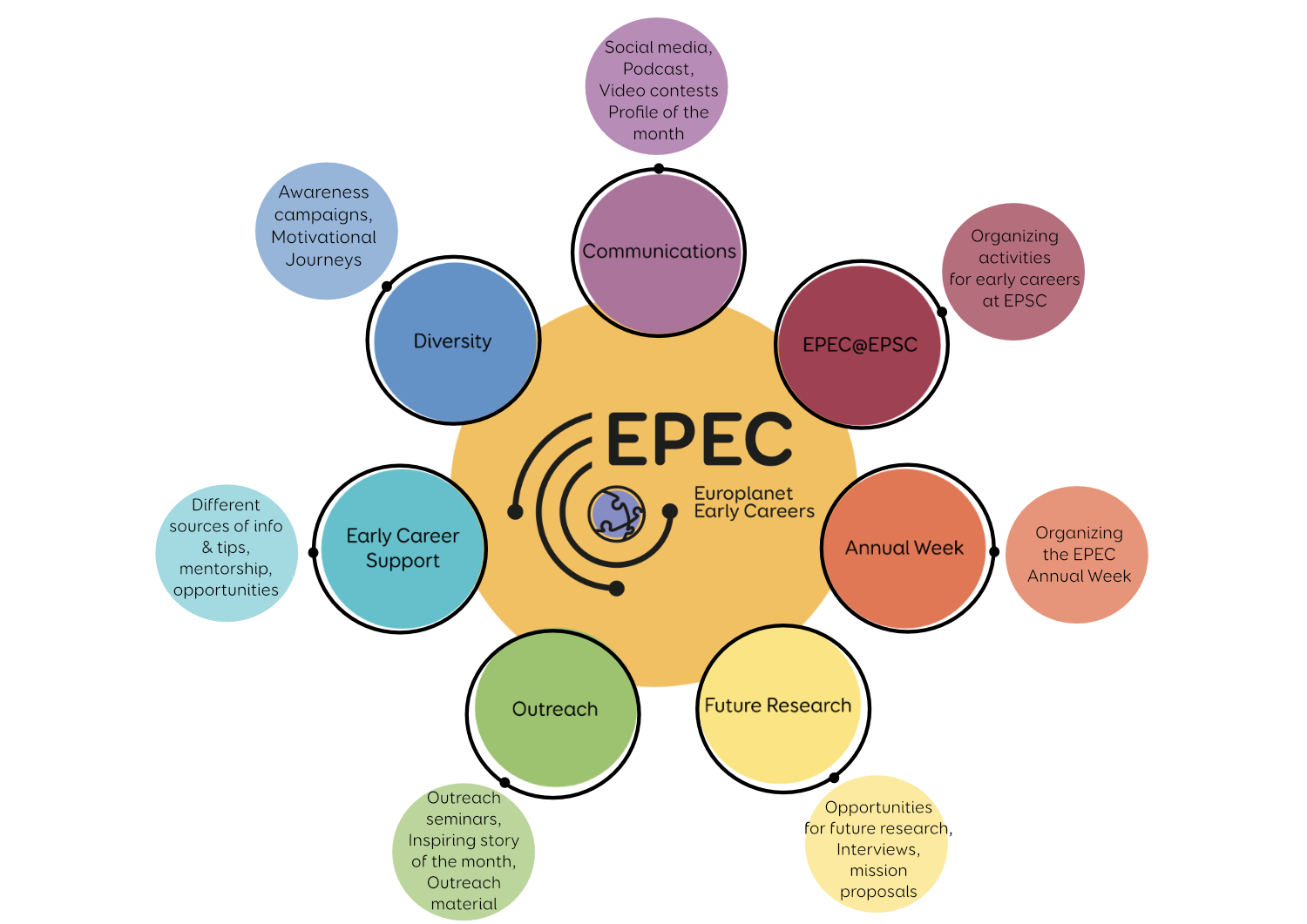
Figure 1: EPEC is divided into 7 Working Groups (black outlined circles), each of them working on different topics (rimless circles).
The WGs are always looking for and welcoming other space enthusiasts who would like to contribute to the EPEC activities. Joining EPEC can be a great opportunity for early-career scientists.
In fact, EPEC offers occasions to meet peers from all across Europe and beyond as well as interact with the broader Europlanet Society committees and members. It is also a great chance to develop new skills of collaboration, leadership, project and team management - all of which will be of great value in their career, academic or not.
Every year, members of EPEC get together for two major events: the EPEC Annual Week (Fig. 2A) and the Europlanet Science Congress (EPSC) (Fig. 2B).
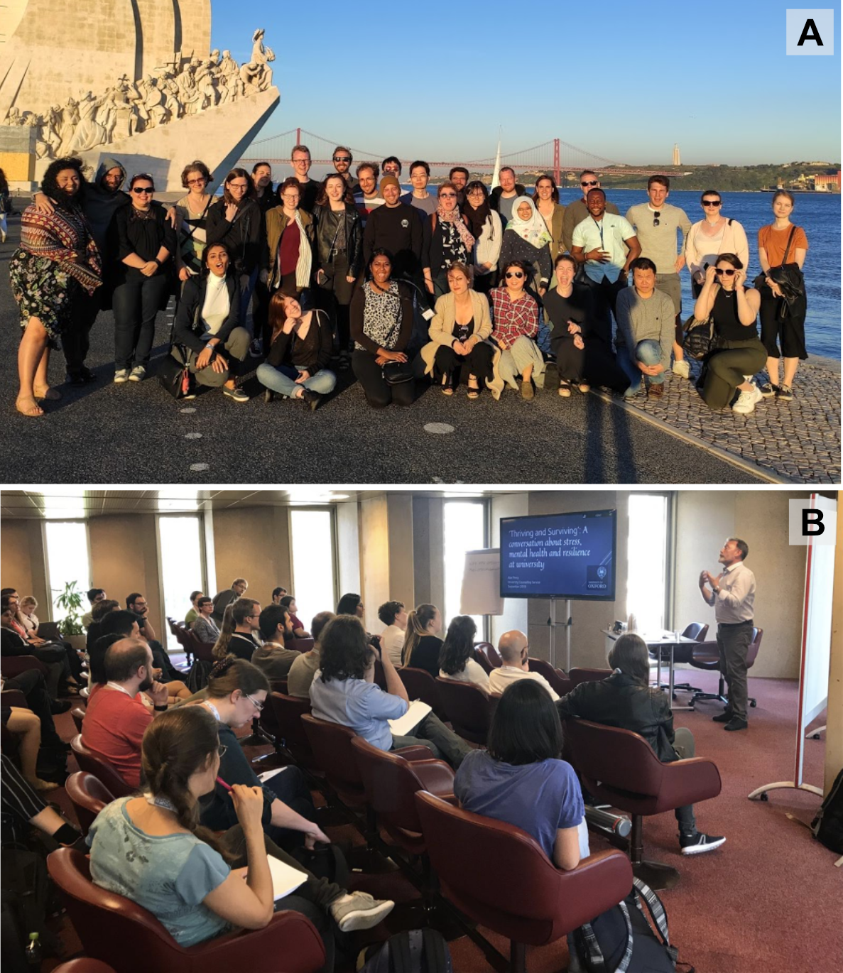
Fig. 2: A) Social event at the 2nd Annual Week, Lisbon, Portugal; B) Early career short courses at EPSC.
The Annual Week is an event that gathers early careers from everywhere in the world, where different seminars and workshops foster a healthy, collaborative, and interactive reflection on topics related to academia and the challenges that early careers face. For the last two years, it has been organized virtually, which reduced our interaction but gave us the unique chance to expand the event in an unprecedented way.
EPSC, on the other hand, is where EPEC members get a chance to present their scientific work to the entire community (including senior scientists) while connecting with other early careers through the EPEC@EPSC program.
Being involved in EPEC means also contributing to making the best of these two events and perhaps creating additional occasions to meet and work together.
Furthermore, EPEC supports early careers with open discussions about mental health (e.g. during the Annual Week), mentoring programs at EPSC, and the Motivational Journeys (Diversity WG) where scientists with different backgrounds share their stories and the obstacles they overcame. We are also going to launch our podcast soon, where we will invite guest speakers to highlight the relevance of a healthy routine during Ph.D. life and provide additional tips for young professionals to learn how to balance working hours and personal space.
This aspect is crucial, we can never stress enough the scientific community's need to be healthy, supportive, and let early careers express their difficulties in such a challenging career.
A few highlights of our current activities include:
- Our Profile Of The Month initiative, to highlight early-career scientists' journeys;
- Our Outreach Stories, that aim to inspire all researchers to share their science with the general public;
- Stairway to Space - EPEC’s brand new podcast;
- Video Contest PlanetaryScience4all, where the participants send a 4-minutes video about their PhD projects, and the winner gets free registration for the next EPSC;
- The early-career program at EPSC - look out for the sessions!
To contact EPEC, message us by email (epec.network@gmail.com).
Europlanet society members (of all career stages) and senior scientists in general are invited to follow EPEC on Twitter (@epec_epn) in order to help EPEC gain visibility among the early careers. More info on EPEC’s activities and how to keep up to date or get involved can be found on our website.
To join EPEC on Slack, scan the QR code:

(for early careers only)
How to cite: Luzzi, E., Belgacem, I., and Mirino, M. and the EPEC committee: The Europlanet Early Career (EPEC) Network: Building a Community to Support Junior Researchers, Europlanet Science Congress 2022, Granada, Spain, 18–23 Sep 2022, EPSC2022-586, https://doi.org/10.5194/epsc2022-586, 2022.
The planetary sciences and related fields are built on the foundation of sharing knowledge and making it accessible to all. In August 2020, Europlanet launched the Mentorship platform with the aim to support early career researchers. The platform is built to help early career scientists to develop expertise, ask questions and discuss career plans with the support of more established members of the planetary community. The success of the mentorship programme highlights the need for this programme and the potential role it can play in developing the individuals within our community who will advance planetary sciences over the coming years. On behalf of mentoring team, I will present the Europlanet mentorship platform and the current status of the programme. Europlanet 2024 RI has received funding from the European Union's Horizon 2020 research and innovation programme under grant agreement No 871149.
How to cite: Stonkute, E.: Mentorship opportunities, Europlanet Science Congress 2022, Granada, Spain, 18–23 Sep 2022, EPSC2022-780, https://doi.org/10.5194/epsc2022-780, 2022.
Astronomy workshops were implemented in the 9th Primary School of Komotini which is an urban school located in the north-eastern part of Greece. The challenge that the school has to tackle is irregular attendance and school dropout. About half of the students come from families that face socioeconomic hardship, live in marginalised settlements in the city and belong to the Muslim minority of Thrace. Their school attendance is characterized by absenteeism that negatively affects the continuity of learning and the development of cognitive and social skills. These are followed by the loss of their self confidence, their alienation in the classroom and the school community. Thus the aim of the school is to be inclusive by accepting and attending to student diversity. Hence, the School administration and teacher staff has decided to implement interdisciplinary various workshops during the whole school year that include Storytelling, Drama, STEAM, Arts, Athletics, Pottery and Gardening. The Astronomy workshops were implemented collaboratively by a teacher, the Arts Teacher and the Music Teacher and in specifically included:
1. Planetarium workshop:
The School has a Planetarium which is a Geodesic Dome made out of white plastic film and a wooden skeleton. It consists of six pentagons, five hexagons and five half hexagons and has a diameter of 5m and height of 3m. It was made in 2018 by children to inspire other children about astronomy. Presentations were given to the whole school, six grades, eight classes, (132 students). The presentations which were focused on the solar system and famous missions were adjusted to their age. Free online videos, Stellarium and NASA’s Eyes were used for the presentations.
2. Music and movement workshop:
Next to the Planetarium is the School’s dance room. After the planetarium presentations the students participated in a music and movement workshop. They listened to sounds of the planets in our solar system and were enhanced by the teacher to kinetically express themselves and guided tο recreate in teams the orbits and rotations of the planets.
3. 3D Printing workshop:
In the ICT Lab students were introduced to 3D printing using Tinkercad a free web app. The School is an eTwinning STEM 3.0 School and was granted a 3D Printer in March. In teams students designed and 3D printed rockets, robotic spacecrafts and space suits.
4. Art workshop:
In the Art room and under the guidance of the Art teacher the students created a collective artwork inspired by the solar system and what they had learnt. Each class contributed by working on a specific part of the synthesis. The artwork is a 3D installation in the space of the corridor of the school that leads to the Planetarium. Polystyrene spheres balls were used for the 3D models of the Sun and planets and were painted with Fluorescent paints that can shine under UV black light. For the scale of the solar system of the artwork the sizes of the planets were taken in consideration in comparison with the Sun.
Acknowledgements
I would like to acknowledge the teachers and students of the 9th Primary School of Komotini.
How to cite: Molla, M., Amperiadis, P., and Kyriazopoulou, G. N.: Astronomy Workshops: Implementation in Greek Primary School, Europlanet Science Congress 2022, Granada, Spain, 18–23 Sep 2022, EPSC2022-1212, https://doi.org/10.5194/epsc2022-1212, 2022.
On 25 June 2022, the third edition of Soapbox Science takes place in Brussels. Soapbox Science is a public outreach platform that was initiated in London, UK in 2011 to promote women in science, and that was spread worldwide since then. Between 2011 and 2018, 40 cities hosted the initiative in not less than 8 countries over 4 continents, and in 2020, despite the pandemic, 56 events were organized in 14 countries around the world.
While the start of Soapbox Science Brussels was challenged by the COVID pandemic, a first virtual event was organised in the fall of 2020 via the YouTube and Facebook platforms [1]. Despite the difficulties related to the sanitary conditions, the first real-life edition of Soapbox Science Brussels finally took place in the heart of the Belgian capital in June 2021, following the standard format prescribed by the international Soapbox Science initiative. This event was a success, both with respect to the response of the scientific community and with regard to the interest of the public during the event. The third edition of Soapbox Science Brussels is currently in preparation, the list of selected speakers is already available and we just launched the campaign for the recruitment of volunteers.
In this communication, we present the development of the Soapbox Science initiative in Belgium. We describe the motivations, challenges, issues and opportunities encountered throughout the process, and how Soapbox Science is gradually taking its place in the Belgian context for the promotion of women in sciences.
Links:
Facebook: https://www.facebook.com/SoapboxScienceBrussels
Twitter account: @SoapboxscienceB
References:
[1] Pham, L. B. S., et al., Soapbox Brussels, une première en Belgique, Science connection nr. 65, August-september 2021;
in French: http://www.belspo.be/belspo/organisation/publ/pub_ostc/sciencecon/65sci_fr.pdf;
in Dutch: http://www.belspo.be/belspo/organisation/publ/pub_ostc/sciencecon/65sci_nl.pdf
How to cite: Piccialli, A., Bingen, C., Pham, L. B. S., Lamort, L., Lefever, K., and Yseboodt, M.: Soapbox Science Brussels: an outreach platform for the promotion of Women in Sciences in Belgium, Europlanet Science Congress 2022, Granada, Spain, 18–23 Sep 2022, EPSC2022-1224, https://doi.org/10.5194/epsc2022-1224, 2022.
ODAA3 | Professional-Amateur collaborations in small bodies, terrestrial and giant planets, exoplanets, and ground-based support of space missions
Introduction
Amateur observations of atmospheric features on the limb or night side of Mars proved their interest ([1], [2]). This led JL, specialist in aurorae, to collaborate with JLD, advanced amateur astronomer, to coordinate ten amateurs for attempting the first observation from Earth of aurora above the limb or on the night side of Mars.
Observations
On Nov. 17th, 2020 (316° solar longitude), one of those amateurs, CP observed a suspect phenomenon over the night side of Mars. We identified an exceptional quality simultaneous observation by EB, over a three-hour timespan (fig. 1). Observation of the data set shows a 3000 km (from equator to South) detached layer on the night side, which seems to rotate with the planet on the day side, casting shadows before disappearing.
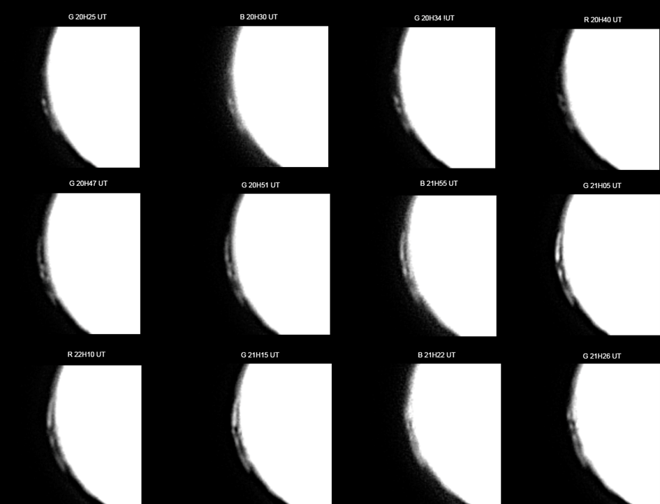
Fig. 1. Detached layer from 20H25 to 21H26 UT through red (R), green (G), and blue (B) filters. The disk is overexposed to better show the phenomenon.
Analysis
This feature could be an aurora, or a cloud system made from dust, H2O or CO2. With MV, specialist in Mars clouds, the collaborative team worked to characterize its altitude, its photometric properties, and its possible composition to determine its type.
a. Altitude
It was determined through several methods, using measures of the apparent position of the features on the images. Assuming the detached layer is seen at the time when the cloud emerges from night side, we used both a simple 2D method (fig. 2) and the 3D equations of [1] on the emergence images’ measures. Another method used the measure of the length of the shadow casted by the features. A last method measured the clouds fronts’ position following the features when it rotates on day side.
Amateurs MD, JLD and EB worked out those different methods which led overall to an altitude of 92 (+30/-16) km.
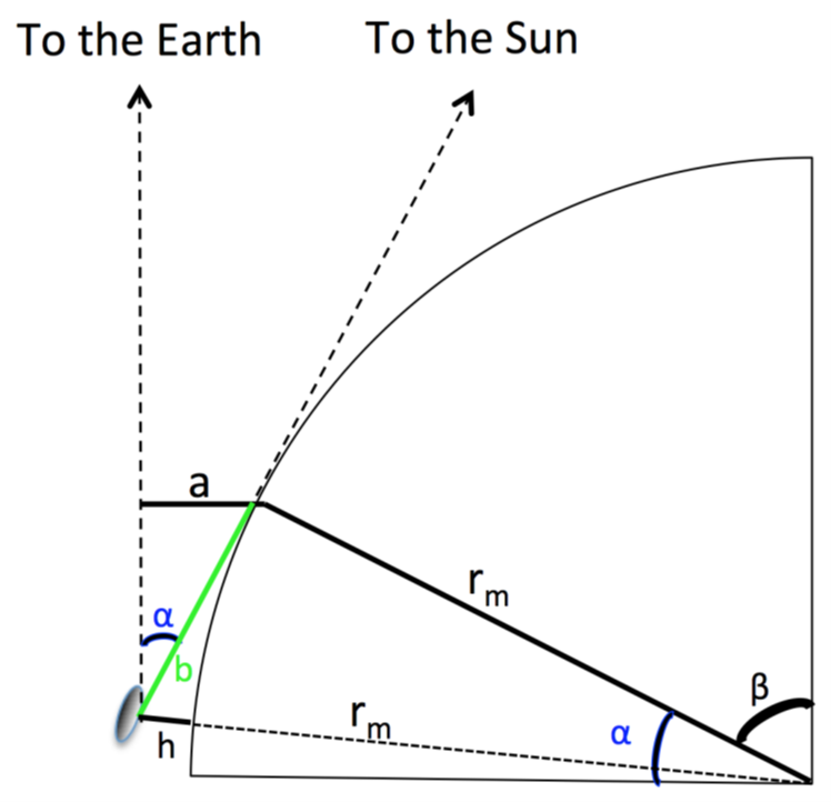
Fig. 2: Detached layer altitude determination with 2D geometric method.
b. Colour profile and albedo
Amateur CP performed UBVRI photometry ([3]) of the planet and the layer. Reference stars observed at the same airmass as the observation were used. Different features were measured (bright and dark terrains, polar cap) as well as the overall globe, and one part of the detached layer. Fig. 3 shows the respective albedos measured, showing how the different zones measured reflects sunlight. The detached layer reflectance is twice brighter in red than in blue (while bright reddish terrain like Amazonis is five times).
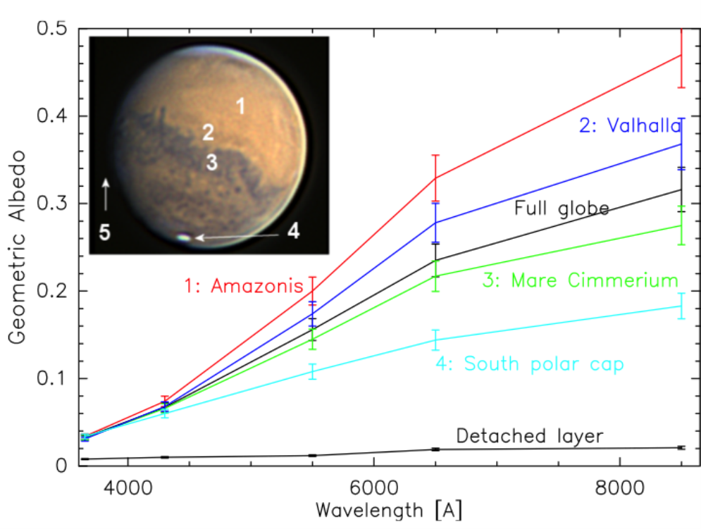
Fig. 3. Albedo of different Martian structures compared to those of the full globe and of the observed detached layer.
c. Size and optical depth of particles constituting the layer
Colour profile shows that the layer scatters light over the whole spectrum, inconsistent with Rayleigh scattering or single wavelength emission, suggesting a layer consisted of dust aerosols or ice crystals.
Professional MV used [4] to model ice scattering reflectance of CO2 and H2O, resulting in fig. 4, showing that the reflectance profile of the layer is compatible with either 1-2µm CO2 or 2(+/-1) µm H2O particle sizes.
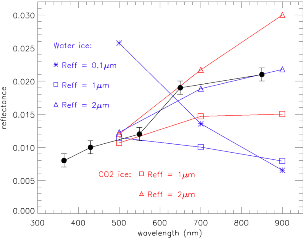
Fig. 4. Spectrum of the detached layer derived from figure 3 (black dots) compared to scattering models of CO2 (red) and H2O (blue) clouds with various ice crystal particle sizes models
Possible interpretation
a. Aurorae
JL predicted ([5]) 140km altitude for blue or green aurorae, and 160km for red aurorae, incompatible with this observation. Blue and green aurorae should be brighter than red ones, which is incompatible with the colour profile we evaluated. The quiet solar conditions on Mars during the observation time is also not compatible with the auroral assumption.
b. Dust clouds
A regional dust storm was present at the opposite side of the detached layer, but its colour is different from our detached layer’s. While high dust layers could reach an altitude of 80km, they are continuous from the ground to high altitude, unlike this observed layer.
c. Water ice
Water ice cloud at altitudes compatible with our observation are possible, in particular during global dust storms but with smaller ice particles (0.1-0.5µm). Nonetheless our observation could be an atypical water ice cloud, i.e. with large grain size despite its high altitude.
d. CO2 ice cloud
Typical mesospheric Martian day side CO2 ice clouds observed by probes are compatible with our observation in terms of particle size, but smaller (only hundreds of km wide), usually earlier in the year. From Mars Climate Database simulation, CO2 frost point could be reached at equator at the altitude of our observation, but at the limit which could be explained by gravity waves or our cloud being on the colder night side. Most of the system is outside of the common place for CO2 clouds (fig. 5). Our observation could be then an atypical CO2 ice cloud.
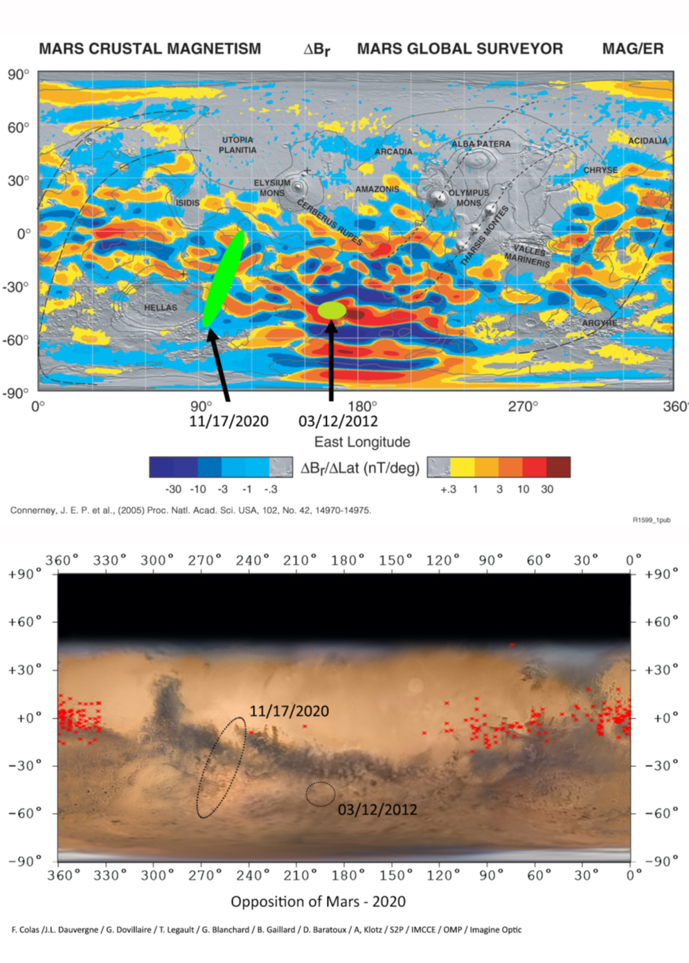
Fig. 5: Localisation of the observation compared to:
Top: Magnetic anomaly with two previous observations ([1]).
Bottom: previous CO2 clouds (red stars) projected on an albedo map.
Conclusion
This observation is located on the West border of the main Martian magnetic anomaly (fig. 5). This could show that cosmic rays, like on Earth or Titan, may have acted, through ionization of the atmosphere’s gas or dust particles, as condensation nuclei for the cloud.
For the first time a huge cloud system was observed from Earth, from its appearance on the night side to its dissipation on the day side only thanks to amateurs’ observations. While looking for aurorae, the study of this observation ruled out this explanation, favouring an ice cloud system either made of water or CO2, but atypical regarding some of its characteristics compared to previous observations. Its localization aside the large magnetic anomaly also indicates a possible explanation of its formation through cosmic rays ([6]).
Bibliography
[1] Sánchez-Lavega, A., et al. 2015, Nature
[2] Sánchez-Lavega, A., et al. 2018, Icarus
[3] Mallama, A. 2007, Icarus
[4] Vincendon, M., et al. 2011, Journal of Geophysical Research (Planets)
[5] Lilensten, J., et al. 2015, Planetary and Space Science
[6] Lilensten, J., et al. 2022, A&A (to be published)
How to cite: Delcroix, M., Lilensten, J., Dauvergne, J.-L., Pellier, C., Beaudouin, E., and Vincendon, M.: Amateur observation of an atypical martian atmospheric feature: when serendipity leads to identify an atypical cloud system, Europlanet Science Congress 2022, Granada, Spain, 18–23 Sep 2022, EPSC2022-43, https://doi.org/10.5194/epsc2022-43, 2022.
- Introduction
The colours of the belts, zones, and individual features of Jupiter are known to encounter significant variations either on short or long time scales. Those variations are the results of chemical or physical changes of the planet's meteorology that are of much interest. In order to try to precisely describe the colours of the planet beyond simple assessments (either visually or from images), the author presents results obtained with tools found in the scientific litterature, to characterize the colours of Jupiter during the apparition of 2021.
Scientific references showing examples of the same kind of work are [1] and [2]
- Method
The planet is imaged with the method of lucky imaging, with a complete set of UBVRcIc plus z', CH4/890, and Y filters. Two cameras are used, one monochrome (ASI290MM from ZWO) and one colour, the ASI462MC, to benefit from its huge sensitivity in the near infrared wavelengths. Wavelet processing is not applied on the images. The geometric albedo of the planet is calculated for each one of the bands, thanks to the method exposed in EPSC2022-20, and the values are exploited with the following presentations. Figures 1 and 2 show photometric images taken respectively on September 6th, 2021, and September 23rd, showing the Great red spot.
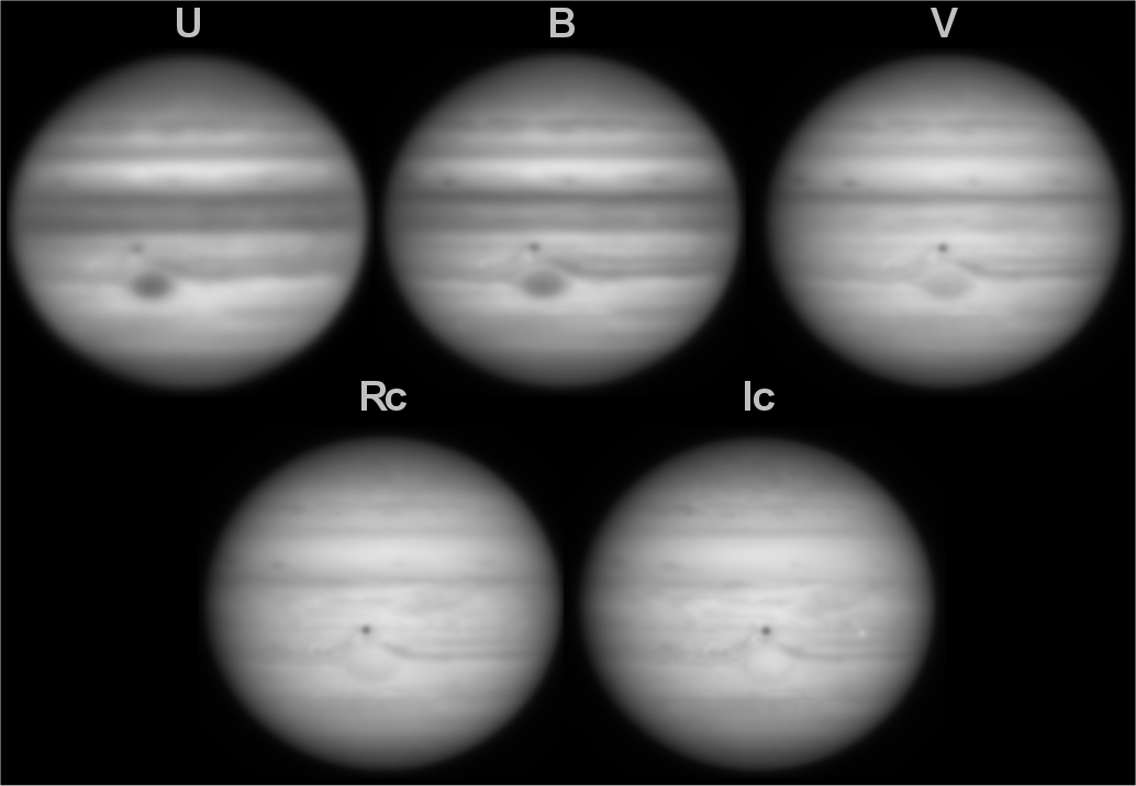
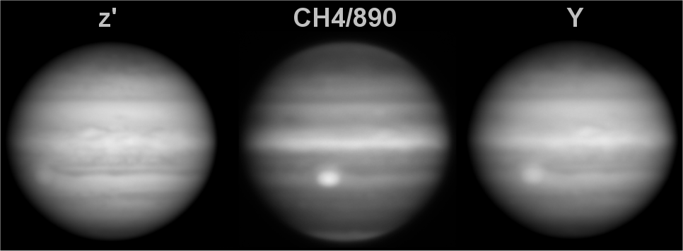
- North-South scans
The goal is to characterize the photometric profile of the planet in direction of the polar axis, for each band of light. For this, images where longitudes estimated to be "representative" of the global state of the planet are used.
Another method would be to use images spanning a long range of longitudes. To diminish the sensitivity of a cut along a single line to local variations (i.e presence of individual spots...) the author used the software RSpec to select a wider range of longitudes around the central meridian (figure 3)
Images are not used directly: they are first sent into WinJupos and mapped onto equirectangular projection with planetographic latitude scale that allows to eliminate the moderate tilt of the globe, when present. The only thing not corrected is the small gradient of light brought by the polar tilt (the "winter" hemisphere being a bit less lit by the Sun). The photometric profile is calibrated in “wavelengths” from 0 to 180, to ease the building of the latitude scale (+90/-90°).
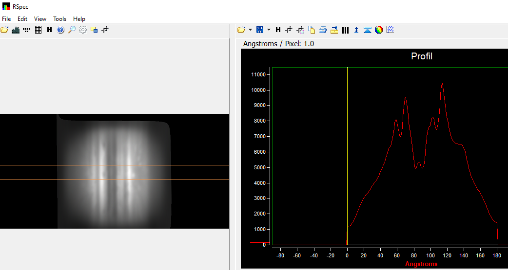
Finally, the profile is calibrated in intensity by calculating the albedo of a well identified region with the same method exposed in point 4 below. On figure 4 is an example of a final scan, all will be visible on the poster.

Ratios of some of those north-south scans can be made to provide colour indices that may reveal additionnal informations. Here is a B-Rc that may forms a good index of the colours of the planet, since the B band is where the maximum of variation occurs, when they are minimal in red (or IR) - figure 5:

- Spectra of individual features or regions
This work also allows to build spectra of individual features or regions, like the Great Red Spot, when measuring their particular albedo on the central meridian. Spectra will then only have a few points, depending on the number of filters used. To measure the albedo of individual features, the author used a circle of know radius (5 or 10 pixels...), noted the value of apparent brightness, and calculated what would be the brightness if this small area would be as large as the disk itself. Then by a simple rule of three, knowing what is the albedo of the global disk, it is possible to calculate the albedo of the feature of interest. An example of such spectra can be found in [2].
- References
[1] Mendikoa, I., Sanchez-Lavega,A., Pérez-Hoyos,S., Hueso,R., Rojas, J-F., Lopez-Santiago,J., "Temporal and spatial variations of the absolute reflectivity of Jupiter and Saturn from 0,38 to 1,7 µm with PlanetCam-UPV/EHU", Astronomy and Astrophysics, vol.607, november 2017.
[2] Simon AA, Wong MH, Rogers JH, Orton GS, De Pater I, Asay-Davis X, Carlson RW, Marcus PS, “Dramatic change in Jupiter's Great Red Spot from spacecraft observations”, The Astrophysical Journal Letters, 797:L31, 2014.
How to cite: Pellier, C.: The colours of Jupiter in 2021, Europlanet Science Congress 2022, Granada, Spain, 18–23 Sep 2022, EPSC2022-51, https://doi.org/10.5194/epsc2022-51, 2022.
Introduction
Taurus Hill Observatory (THO) [1], observatory code A95, is an amateur observatory located in Varkaus, Finland. The observatory is maintained by the local astronomical association Warkauden Kassiopeia. THO research team has observed and measured various stellar objects and phenomena. Observatory has mainly focused on exoplanet light curve measurements, observing the gamma rays burst, supernova discoveries and monitoring [2]. We also do long term monitoring projects [3].
The results and publications that pro-am based observatories, like THO, have contributed, clearly demonstrates that pro-amateurs are a significant resource for the professional astronomers now and even more in the future.
High Quality Measurements
The quality of the telescopes and CCD-cameras has significantly developed in 20 years. Today it is possible for pro-am's to make high quality measurements [4] with the precision that is scientifically valid. In THO we can measure exoplanet transits < 10 millimagnitude precision when the limiting magnitude of the observed object is 15 magnitudes. At very good conditions it is possible to detect as low as 1 to 2 millimagnitude variations in the light curve.
Season 2021 – 2022 Exoplanet Observations Review
A total of about 30 exoplanet observations and transit measurements were made during the observation season 2021/2022. All the measurements have been uploaded to the TRESCA database [5]. In total, about 250 light curve observations have now been sent directly to TRESCA from the Taurus Hill Observatory.
The season highlights that we consider to be most important could be the clear time deviations from the forecasts for a few TESS candidates, and in particular the Qatar-8b transit time deviations. The TOI1582.01b transit was not detected during the predicted period at all, so it differed quite a bit from the predicted one. These observations are presented in the following figures.

Figure 1: TOI1168.01b. The transit occurred about 1.7 hours earlier than predicted. Image: TRESCA.

Figure 2: TOI1455.01b. The transit occurred 1.6 hours earlier than predicted. Image: TRESCA.

Figure 3: TOI1582.01b. Not any clear transit was detected. Image: TRESCA.

Figure 4: TOI2152.01b. The transit occurred about 20 minutes earlier than predicted. Image: TRESCA.

Figure 5: Qatar-8b. The transit happened about three hours later than predicted. Image: TRESCA.
Adapting a New Camera for Measurements
The main equipment throughout the winter were Celestron C-14 SC telescope with a Paramount MEII tripod and an SBIG ST-8XME CCD camera with Baader Bessell BVRI photometric filters.
During the spring 2022, the ASI2600MM Pro CMOS camera was tested for the first time in Taurus Hill Observatory with a Chroma I filter connected to a Meade 16” ACX -telescope (with a Paramount ME tripod) for light curve measurements in the WASP-12b observations on March 31, 2022. At the same time, the object was also detected with an SBIG ST-8XME CCD camera connected to the Celestron C-14 SC -telescope. The results were very similar, so the CMOS camera is well suited for light curve measurements. An interesting feature of the transit of the WASP-12b was that immediately after the actual transit there is a very small dimming of 3 to 5 mmag, which lasts for about 30 minutes. MaxIm DL v6.08 software was used for imaging and image calibration, AIP4Win v2.4.10 software was used for photometric measurements.
The weather was even throughout the dark winter season from August to the end of April. The clearest nights were in March-April. The winter was very rainy overall, there was an exceptional amount of snow. In addition to exoplanet observations, Taurus Hill Observatory focused on comet imaging, DS imaging and the detection of GRB 220101A after-gamma glow, for which circular GCN 31356 [6] was published.
Acknowledgements
The Taurus Hill Observatory will acknowledge all the cooperation partners, Finnish Meteorological Institute and all financial supporters of the observatory.
References
[1] Taurus Hill Observatory website, http://www.taurushill.net
[2] A low-energy core-collapse supernova without a hydrogen envelope; S. Valenti, A. Pastorello, E. Cappellaro, S. Benetti, P. A. Mazzali, J. Manteca, S. Taubenberger, N. Elias-Rosa, R. Ferrando, A. Harutyunyan, V.-P. Hentunen, M. Nissinen, E. Pian, M. Turatto, L. Zampieri and S. J. Smartt; Nature 459, 674-677 (4 June 2009); Nature Publishing Group; 2009.
[3] A massive binary black-hole system in OJ 287 and a test of general relativity; M. J. Valtonen, H. J. Lehto, K. Nilsson, J. Heidt, L. O. Takalo, A. Sillanpää, C. Villforth, M. Kidger, G. Poyner, T. Pursimo, S. Zola, J.-H. Wu, X. Zhou, K. Sadakane, M. Drozdz, D. Koziel, D. Marchev, W. Ogloza, C. Porowski, M. Siwak, G. Stachowski, M. Winiarski, V.-P. Hentunen, M. Nissinen, A. Liakos & S. Dogru; Nature - Volume 452 Number 7189 pp781-912; Nature Publishing Group; 2008
[4] Transit timing analysis of the exoplanet TrES-5 b. Possible existence of the exoplanet TrES-5 c; Eugene N Sokov, Iraida A Sokova, Vladimir V Dyachenko, Denis A Rastegaev, Artem Burdanov, Sergey A Rusov, Paul Benni, Stan Shadick, Veli-Pekka Hentunen, Mark Salisbury, Nicolas Esseiva, Joe Garlitz, Marc Bretton, Yenal Ogmen, Yuri Karavaev,Anthony Ayiomamitis, Oleg Mazurenko, David Alonso, Sergey F Velichko; Monthly Notices of the Royal Astronomical Society, Volume 480, Issue 1, October 2018, Pages 291–301, https://doi.org/10.1093/mnras/ sty1615
[5] TRESCA; var2.astro.cz/tresca/transits.php?pozor=Veli-Pekka Hentunen&object=&page=1&lang=cz
[6] Hentunen V-P, Nissinen M, Heikkinen E; GCN 31356; https://gcn.gsfc.nasa.gov/gcn/gcn3/31356.gcn3
How to cite: Haukka, H., Hentunen, V.-P., Nissinen, M., Salmi, T., Aartolahti, H., Juutilainen, J., Heikkinen, E., and Vilokki, H.: Taurus Hill Observatory Season 2021 – 2022 Exoplanet Observations Review, Europlanet Science Congress 2022, Granada, Spain, 18–23 Sep 2022, EPSC2022-67, https://doi.org/10.5194/epsc2022-67, 2022.
The cloud discontinuity of Venus is a planetary-scale phenomenon known to be recurrent since, at least, the 1980s. It was initially identified in images from JAXA’s orbiter Akatsuki. This disruption is associated to dramatic changes in the clouds’ opacity and distribution of aerosols and is interpreted as a new type of Kelvin wave. The phenomenon may constitute a critical piece for our understanding of the thermal balance and atmospheric circulation of Venus. The reappearance on the dayside middle clouds four years after its last detection with Akatsuki/IR1 is reported in this work. We characterize its main properties using exclusively near-infrared images from amateur observations for the first time. The discontinuity exhibited tempοrаl variations in its zonal speed, orientation, length, and its effect over the clouds’ albedo during the 2019/2020 eastern elongation in agreement with previous rеρorts. Moreover, amateur observations are compared with simultaneous observations by Akatsuki UVI and LIR confirming that the discontinuity is not visible on the upper clouds’ albedo or thermal emission. While its zonal speeds are faster than the background winds at the middle clouds, and slower than winds at the clouds’ top, it is evidencing that this Kelvin wave might be transporting momentum up to upper clouds.
How to cite: Kardasis, E., Peralta, J., Maravelias, G., Imai, M., Wesley, A., Olivetti, T., Naryzhniy, Y., Morrone, L., Gallardo, A., Calapai, G., Camarena, J., Casquinha, P., Kananovich, D., MacNeill, N., Viladrich, C., and Takoudi, A.: Results from the professional-amateur collaboration to investigate the Cloud Discontinuity phenomenon in Venus’ atmosphere, Europlanet Science Congress 2022, Granada, Spain, 18–23 Sep 2022, EPSC2022-208, https://doi.org/10.5194/epsc2022-208, 2022.
Introduction
The extended portion of NASA’s Juno mission began on 1 August 2021 and will continue through September 2025. The extended mission expands Juno’s science goals beyond those of the prime mission, as noted at the last EPSC (Orton et al. EPSC2021-58). Atmospheric studies will continue to be among the foremost of science goals and an area in which the world-wide community of Jupiter observers can provide significant contextual support. Juno’s remote-sensing observations will take advantage of the migration of its closest approaches (“perijoves” or PJs) toward increasingly northern latitudes. The observations should include close-ups of the circumpolar cyclones and semi-chaotic cyclones known as “folded filamentary regions”. A series of radio occultations will provide vertical profiles of electron density and the neutral-atmospheric temperature over several atmospheric regions. The mission will also map the variability of lightning on Jupiter’s night side.
Physical Details of the Mission
The sequence of orbits and key investigations of the primary and extended missions are shown in Figure 1. We note that on PJ34, the orbital period was reduced from 53 days to 43-44 days. It will be reduced shortly after this meeting on PJ45 to 38 days and again on PJ57 to ~33 days.
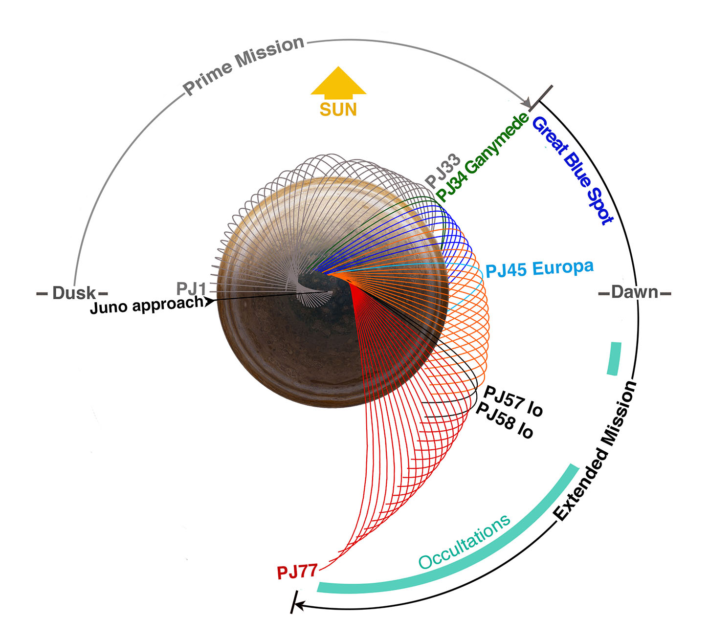
Figure 1. Progression of Juno orbits viewed from above Jupiter’s north pole with respect to local time of day. “PJ” designates a “perijove”, the closest approach to Jupiter on each numbered orbit. Following a Ganymede flyby on PJ34 (green orbit), the orbital period decreased from 53 days to 43-44 days (green + blue orbits). The “Great Blue Spot” (blue) orbits map an isolated patch of intense magnetic field. Following a close Europa flyby on PJ45 (aqua orbit), the period will decrease to ~38 days (orange orbits). Following close flybys of Io on PJ57 and PJ58 (black orbits) the period will decrease to ~33 days (red orbits). In reflected sunlight, Jupiter will mostly appear as a crescent at perijoves following PJ58.
Some characteristics of perijoves of the extended mission are shown in Table 1. We caution that while the day of year for the perijoves is reasonably fixed, the exact times may change by hours in either direction and the longitudes will change accordingly. Timing for later orbits up to PJ76, may be affected by currently unmodeled anomalies in satellite masses that could change dates and times.
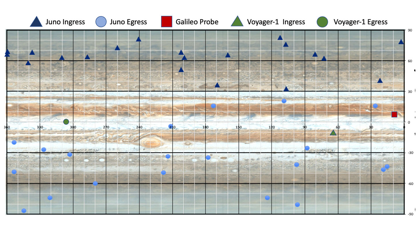
Figure 2. Expected latitudes and longitudes to be measured by the 20 radio occultations of the Juno spacecraft between PJ52 and PJ77. Locations of ingress lie largely in the northern hemisphere - locations of egress in the southern hemisphere. Locations of the Galileo Probe and Voyager-1 radio occultations are also shown for reference.
Role of Amateur Astronomers
We’ve noted in the past at previous EPSC meetings how amateurs can contribute to the Juno mission via their collective world-wide 24/7 coverage of Jupiter. This applies also to the cadre of professional astronomers supporting the Juno mission and its reconnaissance of the Jupiter system over a broad spectral range. In the past, these have alerted observers to strong interactions between the Great Red Spot and smaller anticyclones (Sanchez-Lavega et al. 2021. J. Geophys. Res. 126, e006686) and the occurrence and evolution of prominent and unusual vortices, such as “Clyde’s spot” (Hueso et al. 2022. Icarus 380,114994). During the last apparition, observations were made with the NASA Infrared Telescope Facility (IRTF) that showed slow-moving bright patches in the Equatorial Zone (EZ) that were observed more continuously among the amateur community with 890-nm (“methane”) filters. We also identified an intense 5-µm spot detected using IRTF imaging that coincided with an unusually dark spot in amateur methane-filtered images. The continued tracking of outbreaks in the southern part of the North Equatorial Belt (NEB) also greatly informed the Juno team and supporting astronomers regarding the systematic longitudinal distribution of outbreaks and the range of atmospheric features they generate. A perijove-by-perijove summary of Juno-supporting observations – past, current and planned - is available at the following web site: https://www.missionjuno.swri.edu/planned-observations.
We want to emphasize that by PJ50, Juno’s perijoves will have migrated to a part of the planet that is not in sunlight. At that point and through the end of the mission, images from this community will be extremely useful to order to provide a context for several investigations. One of these will be chief on JunoCam’s agenda during this part of the mission: searches for lightning. But similar contextual information will be sought for measurements of thermal emission from the JIRAM instrument’s high-resolution maps of 5-µm emission, as well as the Microwave Radiometer (MWR) measurements of thermal emission from the deep atmosphere. Although the highest spatial resolution from these instruments will include high northern latitudes (see Table 1) that are not well resolved by small telescopes, measurements of mid-northern latitudes will continue to be made when JunoCam will not be able to provide a visual context.
Table 1. Current estimates for Juno extended mission perijoves PJ45-PJ53. Timing for orbits PJ54 onward may be affected by currently unmodeled anomalies in satellite masses that could change dates and times. Accordingly we list perijove times to the nearest half hour and longitudes to the nearest 10°. Orton et al. (EPSC2021-58) presented information for previous perijoves.
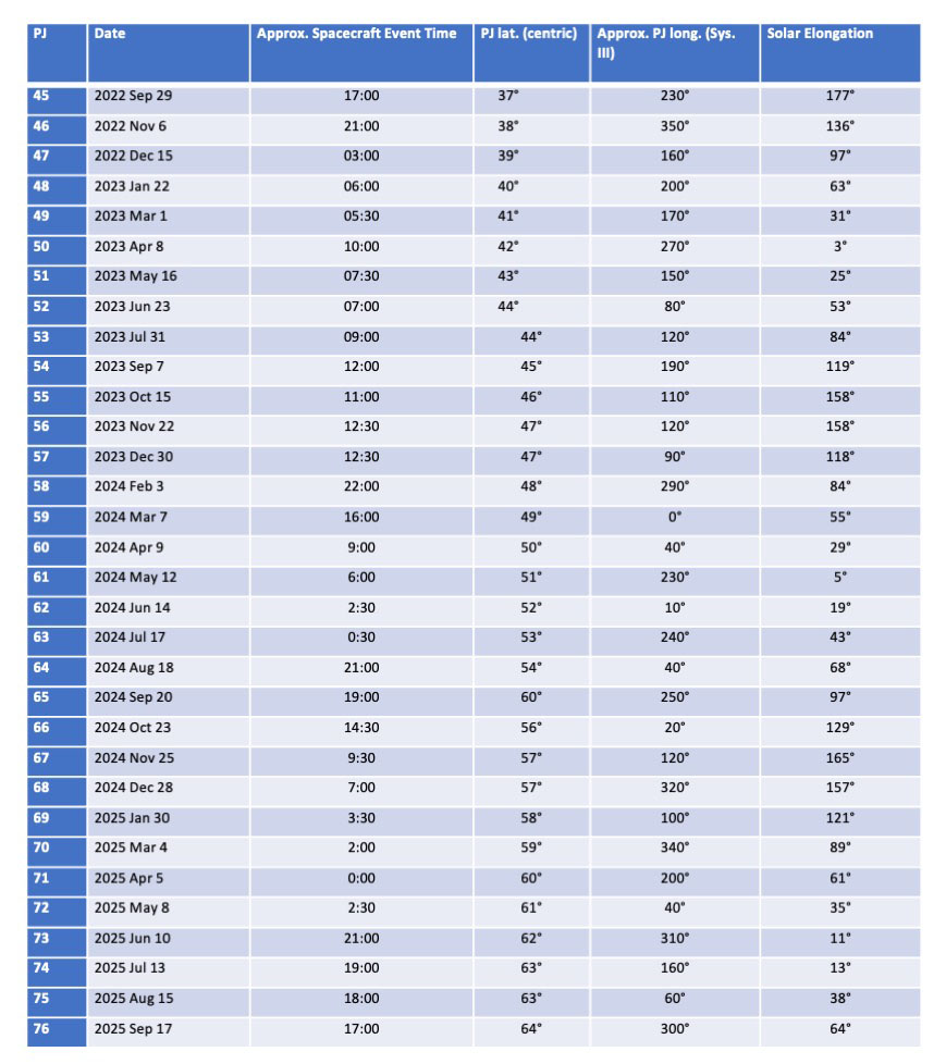
How to cite: Orton, G., Momary, T., Brueshaber, S., Hansen, C., Bolton, S., and Rogers, J.: The Juno Extended Mission: A Call for Continued Support from Amateur Observers, Europlanet Science Congress 2022, Granada, Spain, 18–23 Sep 2022, EPSC2022-769, https://doi.org/10.5194/epsc2022-769, 2022.
Abstract
As a potential pro-am complement to professional Jovian ammonia observations, continuum-divided 645 nm ammonia absorption observations were made using a small telescope. This paper presents highlights of observations during 2020 and 2021. If this low-cost technique can be promulgated among amateurs, then routine atmospheric monitoring of Jupiter would reach a new level of sophistication.
Introduction
New microwave and MIR observations, along with models, reveal much about Jupiter's ammonia cycle at depth. For example, the Juno MWR instrument permits the retrieval of the average ammonia abundance to a depth of 100 bar [1]. Additional recent work has used MIR observations to probe to depths of several bars [2-3]. Similarly, there have been efforts at global retrievals using hyperspectral imaging in the optical and NIR [4-5]. Complementing these efforts have been notable improvements in the understanding of the ammonia optical and NIR absorption bands [6]. Slit spectrometry data extend an already long record [7]. Finally, recent work has shown the efficacy of imaging Jovian upper tropospheric features in the 645 nm ammonia absorption band [8], which the current paper expands upon.
Observations
Thirty-nine usable observing sessions were carried out during 2020-2021 from the author’s observatory in Denver, Colorado. Fig. 1 shows the observations versus System I longitude. It also depicts Juno perijoves. During July and September 2020 observations overlap with the longitudes observed by Juno on PJ28 and PJ29. The best adjacent observations in 2021 occurred in October (PJ37). Also, near Juno perijove (PJ36), the System 1 longitude range of 140-180 degrees was observed multiple times. This allows for observing the evolution of features in the Equatorial Zone (EZ).
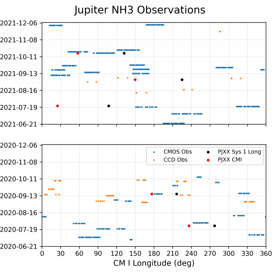
Figure 1: Observing sessions in 2020 (bottom) and 2021 (top). Individual images contributing to ammonia absorption observations are shown (CMOS: blue; CCD: orange). Juno perijove longitudes (Sys. 1) and Earth-facing central meridians (Sys. 1) at perijove are indicated in black and red respectively.
Highlights
Fig. 2 shows the NEB has reduced ammonia absorption, the EZ is enhanced, and the GRS is reduced. Note the correlation and lack of correlation with obvious visible features. There is a reduction correlated with the GRS, but the reduced absorption region from about 15-25N includes both bright and dark features.
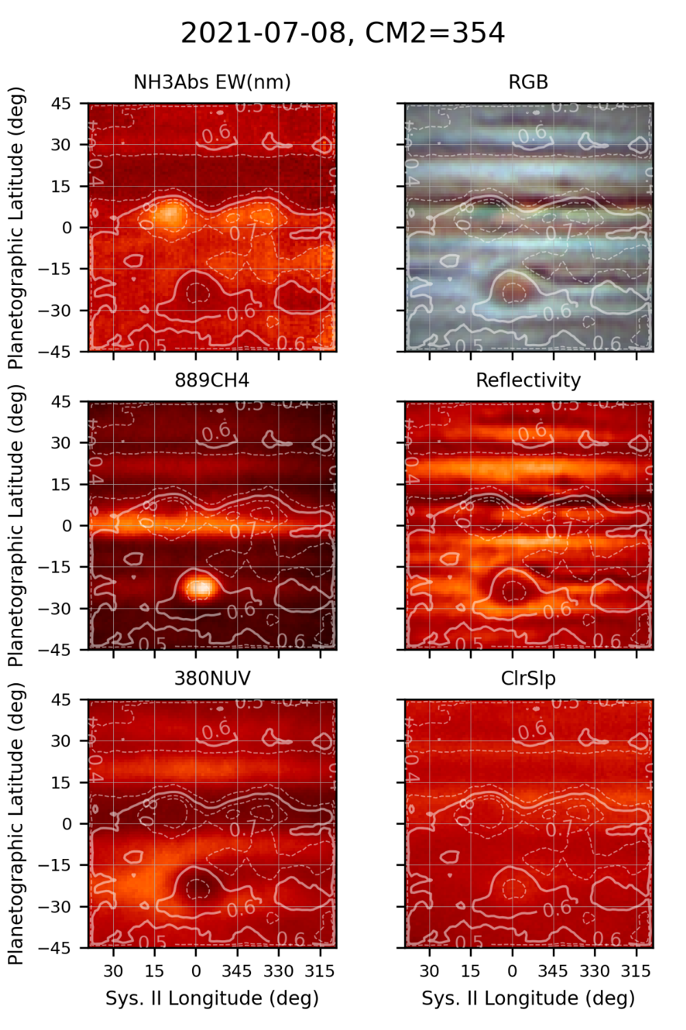
Figure 2: Ammonia absorption and context maps. Brightness scaling is arbitrary and adjusted for visual effect. Contour levels are estimated ammonia absorption equivalent width in nm. “ClrSlp” is relative color slope with redder areas shown as brighter.
Fig. 3 shows the EZ and NEB, including ammonia absorption enhancements near plumes and dark features. Dark features look deep into the atmosphere and the bright plumes represent high clouds.
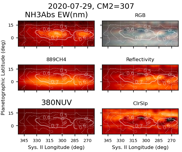
Figure 3: Same as Figure 4 but focused on the northern EZ.
The GRS is shown from July through September 2021 in Fig. 4. Ammonia absorption is reduced over the GRS due to the high-altitude scattering layer there. This reduction has also been noted in spectroscopic observations [7].
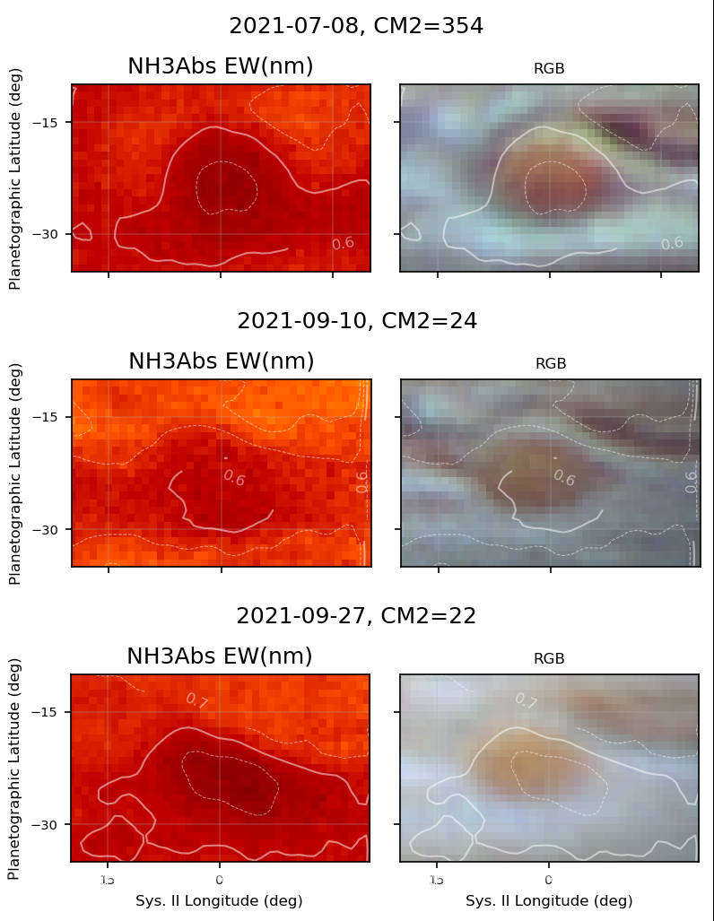
Figure 4: Reduced ammonia absorption over the Great Red Spot at three epochs in 2021.
Retrieval Potential
A scatter plot of 889 nm brightness versus 645 nm NH3 equivalent width (Fig. 5) shows the distributions of different latitude bands. High brightness in the methane band indicates higher cloud tops, which leads to a shorter absorption path. Thus, the GRS (high brightness red ‘tail’ in the 15-30S band) has a high reflecting layer. The ammonia EW is low, consistent with the short absorption path. The NEB (brown) shows uniformly low methane brightness, indicating deeper cloud tops, but also shows low ammonia absorption. This supports an actual depletion in ammonia abundance.
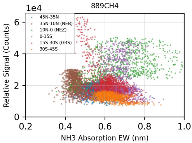
Figure 5: Scatter plot 889 nm methane relative signal versus 645 nm ammonia equivalent width for different meridional bands (2021-07-08, CM2 354 deg).
The scatter plot analysis suggests that a simple Reflecting Layer Model might provide meaningful first-order retrievals of atmospheric properties [9]. The goal during 2022 will be to retrieve reflectivity, cloud top pressure, and ammonia abundance by extending this model. In addition, observations will be shared on amateur collaboration websites.
Summary and Conclusion
This paper highlights two years of continuum-divided ammonia absorption imaging of Jupiter. The method shows detail inaccessible with other imaging techniques. The observations will be tested for utility in a simple atmospheric retrieval model and will be shared during the 2022 apparition.
References
[1] Guillot, T., et al. (2020), Storms and the Depletion of Ammonia in Jupiter: II. Explaining the Juno Observations, Journal of Geophysical Research (Planets), 125, e06404.
[2] Fletcher, L. N., et al. (2020), Jupiter's Equatorial Plumes and Hot Spots: Spectral Mapping from Gemini/TEXES and Juno/MWR, Journal of Geophysical Research (Planets), 125, e06399.
[3] Fletcher, L. N., et al. (2021), Jupiter's Temperate Belt/Zone Contrasts Revealed at Depth by Juno Microwave Observations, Journal of Geophysical Research (Planets), 126, e06858.
[4] Braude, A. S., P. G. J. Irwin, G. S. Orton, and L. N. Fletcher (2020), Colour and tropospheric cloud structure of Jupiter from MUSE/VLT: Retrieving a universal chromophore, Icarus, 338.
[5] Dahl, E. K., N. J. Chanover, G. S. Orton, K. H. Baines, J. A. Sinclair, D. G. Voelz, E. A. Wijerathna, P. D. Strycker, and P. G. J. Irwin (2021), Vertical Structure and Color of Jovian Latitudinal Cloud Bands during the Juno Era, The Planetary Science Journal, 2, 16.
[6] Irwin, P. G. J., N. Bowles, A. S. Braude, R. Garland, S. Calcutt, P. A. Coles, S. N. Yurchenko, and J. Tennyson (2019), Analysis of gaseous ammonia (NH3) absorption in the visible spectrum of Jupiter - Update, Icarus, 321, 572.
[7] Teifel', V. G., V. D. Vdovichenko, P. G. Lysenko, A. M. Karimov, G. A. Kirienko, N. N. Bondarenko, V. A. Filippov, G. A. Kharitonova, and A. P. Khozhenets (2018), Ammonia in Jupiter's Atmosphere: Spatial and Temporal Variations of the NH3 Absorption Bands at 645 and 787 Nm, Solar System Research, 52, 480.
[8] Hill, S. (2021), Experimental Observations of Jupiter in the Optical Ammonia Band at 645 nm, edited, pp. EPSC2021-2260.
[9] Mendikoa, I., S. Pérez-Hoyos, and A. Sánchez-Lavega (2012), Probing clouds in planets with a simple radiative transfer model: the Jupiter case, European Journal of Physics, 33, 1611.
How to cite: M Hill, S. and Rogers, J.: Jupiter Ammonia Absorption Imaging: Highlights 2020-21, Europlanet Science Congress 2022, Granada, Spain, 18–23 Sep 2022, EPSC2022-802, https://doi.org/10.5194/epsc2022-802, 2022.
I this talk I will present the process to get observations on a Europlanet network telescope for an exoplanet transit. The steps of obtaining and also analysing the exoplanet transit light curve will be described. These data are used for the future Ariel space mission organised by ESA. Moreover, the talk will describe the process of writing the proposal for the request of the observation and in the particular case to the Instituto de Astrofísica de Canarias. In parallel, I will explain the way to obtain the funding for the telescope cost by Europlanet organization. Then I will go through the observations themselves and the live decisions regarding signal to noise, exposure time and so on in order to maximize the success probability. Then a report regarding the progress of the observation(s) is written and sent to the organisers. After the part of obtaining the observation, I will describe he process of analysing the images with the ExoClock HOPS software. Details will be provided on how to work with it, how to choose comparison stars, how to get the best light curve and to determine the exact moments of the ingress of the transit and the egress of it. Once the light curve is produced, it is uploaded in the ExoClock website and after reviewing it gets published at the ExoClock database. I would like to highlight that main partners in this work are two women, what is not so common in this field.
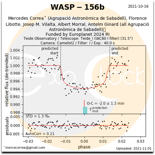
How to cite: Libotte, F. and Correa, M.: Exoplanet observations: amateur experience from the Europlanet Telescope network, Europlanet Science Congress 2022, Granada, Spain, 18–23 Sep 2022, EPSC2022-945, https://doi.org/10.5194/epsc2022-945, 2022.
Comet observation and analysis is an area where amateur observers can make a significant contribution. Their observations allow regular monitoring of comets, alerting the professional community to interesting events, and providing raw data to supplement professional data. The links between the professional and amateur communities are therefore very important.
Comet analysis is challenging. Encouraging the community to agree consistent methodologies, and parameters for analysis, will result in a more robust data set for monitoring and analysis.
The last comet workshop was held in 2015 and the comet community welcomed the opportunity to meet again.
The main aims and objectives of the workshop were agreed, following consultation, to be:
- To foster stronger working relationships and cooperation within the professional and amateur comet community, based on a shared understanding of the challenges and opportunities.
- To take stock of where cometary science stands post-Rosetta and how Pro-Am observations fit into potential future research.
- To draw together the various strands of work currently going on within the community, particularly on coordination, techniques, standards and archiving and agree the way forward.
- To consider how best to encourage, and equip, more people to become involved in the study of comets, whether directly through observation (including access to the Europlanet Telescope Network), or through analysis of online data sources.
- To explore how cometary science can be used in outreach and education.
It was also agreed that speakers should include a wide range of amateurs, students and professional astronomers, and that allowing ample time for panel-led discussions was very important. The panels should include specialists and society representatives.
An accessible location was chosen, the Stefanik Observatory in Prague, along with online access.
We will report on the outcomes from the hybrid workshop and the proposed next steps.
Acknowledgements
The workshop has been organised in cooperation with Europlanet 2024 Research Infrastructure (RI), the British Astronomical Association, Planetum Prague, and the Czech cometary community SMPH.
Europlanet 2024 RI has received funding from the European Union’s Horizon 2020 research and innovation programme under grant agreement No 871149.
How to cite: Usher, H., Snodgrass, C., Biver, N., Kargl, G., Tautvaišienė, G., James, N., Walter, F., and Černý, J.: Strengthening Pro-Am Comet Community Cooperation: Report on Europlanet Pro-Am Workshop (10-12 June 2022) , Europlanet Science Congress 2022, Granada, Spain, 18–23 Sep 2022, EPSC2022-1135, https://doi.org/10.5194/epsc2022-1135, 2022.
The technological progress of electronic, optic and mechanic domains brought high performance astronomy equipment at affordable prices for student and amateur astronomers. As a result, the amateur astronomers contribution to scientific publications has increased exponentially (e.g. Knapen 2011, Mousis et al. 2013). For example, various transient events and long term monitoring of celestial bodies can be observed with a telescope having an aperture of 0.2-0.5 m, and CCD or CMOS detector (e.g. Gherase et al. 2015).
Also, such equipment allows to attract students for a career in science and technology. The "astronomical concepts and images have universal appeal, inspiring wonder and resonating uniquely with human questions about our nature and our place in the universe" (National Academies Press, 2021). Thus, we believe that fundamental concepts related to the scientific method can be learned by a student who comes with questions related to celestial bodies, makes his own observations, processes the acquired images, analyzes the obtained data, and then presents his new findings to the community.
Motivated by these facts we developed T025 – BD4SB telescope. The acronym is represented by the aperture of the telescope (0.25 m) and the project through which we financed its acquisition (Big Data for Small Bodies). We installed this robotic telescope on the roof of the old Bucharest Astronomical Institute. This location corresponds to Minor Planet Center observatory code 073. Here we describe the setup, highlight some of the obtained results, and we discuss the perspectives.
Setup
The components of the instrument are: a Lacerta 250/1000 Newtonian telescope mounted on a Sky Watcher EQ6 Pro Go-To equatorial mount, a 14 bit QHY 294M Medium Size Cooled CMOS Camera, and a mini PC Beelink computer for controlling the setup. Including the auxiliaries (guiding telescope and camera, cables, and adapters) the cost of this setup was about 6k euros (as of 2020). Additionally, a permanent internet connection and electrical power are needed. This setup gives a field of view of 44x66 arcminutes, and a projected pixel size of 0.956 arcesc/pixel. 
Fig.1 The T025 – BD4SB prepared for observations.
The full control of this instrument is made using the Nighttime Imaging 'N' Astronomy – NINA software interface (https://nighttime-imaging.eu/). The data reduction is performed using the IRAF and its PyRAF counterpart in Python. We designed a general pipeline based on Python scripts to perform the bias and flat corrections, to find the astrometric solution using Source Extractor and SCAMP software, and to retrieve the photometry of all sources in the images. All data is stored on a dedicated server and we intend to make it online available. Additionally, we use Astrometrica, Tycho, MPO Canopus and HOPS (HOlomon Photometric Software) programs for specific tasks.
The median magnitude limit is ~20 V band magnitude. Because we are observing from a light polluted area (although we are located in the Carol Park from Bucharest, and the area is surrounded by a lot of trees), the sky brightness varies between the seasons, and consequently the limiting magnitudes are in the range of 19 – 20.7. These limiting magnitudes could be obtained in about ~15 min total exposure time, and they are imposed by the brightness of the sky. The median seeing is ~2.8 arcsec, but the range of variability is 1.8 -4 arcsec.
Observations and results
The objectives of our project is to obtain high quality astrometric and photometric data which can be used for university student projects (including those for bachelor thesis and master thesis) and for participating in scientific publications. Thus, we make the following types of observations: 1) astrometric observations of asteroids and comets, prioritizing the newly discovered NEAs or those with uncertain orbits; 2) photometric observations of Solar System bodies with the aim to obtain accurate light-curves for deriving the spin-properties and their shape; 3) the occultations which are performed in various international campaigns; 4) follow-up of various exoplanets transits; 5) light-curves of variable stars.
We reported more than 100 observations to the Minor Planet Center. These include three confirmations of newly discovered NEAs, and the participation to the IAWN campaign for 2019 XS (Farnochia et al. 2022). We obtained the light-curves and rotation-periods for four NEAs, designated 4660, 153591, 12711, 2019 XS. We obtained more than 65 hours of data for asteroid (4660)Nereus which (Mansour et al. EPSC 2022).
One of the challenging observation was obtained during the nights of November 10-11, 2021 for the NEA 2019 XS (absolute magnitude of 23.87). The object moved with an apparent rate of 20-30 arcsec/min, so we could use an exposure time of 5-10 sec and we had to change the field several times during the night. The result (Fig. 2) shown strong evidences that 2019 XS is a tumbling asteroid. 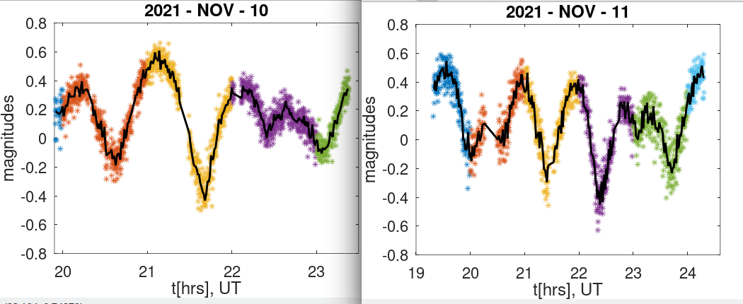
Fig.2 The light-curves obtained for 2019 XS. Colors correspond to different fields and the black line is a median of every 9 points.
Another result we highlight is the four transits we observed for exoplanets TOI-1259Ab, WASP-10b, HAT-P-3b. The lightcurves were submitted to TRESCA-Exoplanets (http://var2.astro.cz/EN/tresca/) database. They show that such setup can obtain photometric measurements with a precision in the range of mili-magnitudes for targets as faint as 14. 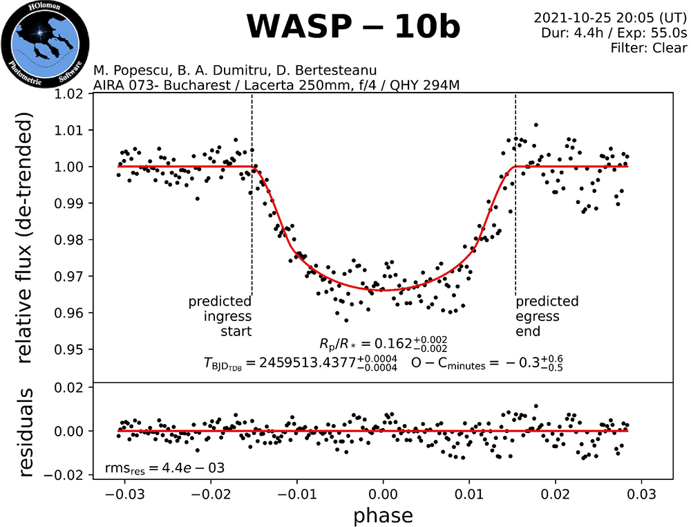
Fig.3 The transit of WASP-10b exoplanet .
Acknowledgments
This work was supported by a grant of the Romanian National Authority for Scientific Research – UEFISCDI, project number PN-III-P1-1.1- TE-2019-1504, contract number TE 173/23/20/2002.
References
1. Johan H. Knapen 2011, Proceedings of ”Stellar Winds in Interaction”
2. Mousis et al. 2014, Experimental Astronomy, Volume 38, Issue 1-2, pp. 91-191
3. Radu-Mihai Gherase et al. 2015, Romanian Astronomical Journal, Vol. 25, No. 3, p.241
4. Astronomy and Astrophysics in the New Millennium; The National Academies Press. https://doi.org/10.17226/9839
5. Farnochia et al. 2022, PSJ, accepted
How to cite: Nicolae Berteșteanu, D., Popescu, M., Mihai Gherase, R., Alexandru Mansour, J., Alexandru Dumitru, B., Stanciu, B., Perrotta, A., H. Naiman, M., Blagoi, O., Dumitru, T., and Lupoae, A.: The T025 – BD4SB a pro-am collaboration for planetary sciences, Europlanet Science Congress 2022, Granada, Spain, 18–23 Sep 2022, EPSC2022-1222, https://doi.org/10.5194/epsc2022-1222, 2022.
ODAA4 | Public engagement via live online astronomy events: Sharing experiences, looking ahead
In 2009 Elisa, a student of Physics and Advanced Technologies, could not access the dome of the University of Siena Astronomical Observatory because she is forced on a wheelchair by disability. “Advanced technologies” helped her, though. Between 2010 and 2012 the Observatory instrumentation was completely updated, but, most importantly, was fully automated, and made remotely controllable trough an Internet connection.
Since 2012 the Observatory is a laboratory where university and high-school students learn to study the starry sky and how to use the most recent instruments and technologies for astronomical image acquisition and analysis. Through this acquired knowledge, small projects focused on asteroids, variable stars and extrasolar planets research can be conducted by a wide range of students, academic organizations and enthusiast citizens.
In August 2015, Sara Marullo, a student in Physics and Advanced Technologies at the University of Siena who lived very far from the observatory, managed to conduct a series of observations, required by her internship, from her home. During an asteroid study session, in a case of perfect serendipity, she discovered a peculiar binary star. A few months later, that discovery of a new double star became the topic of her thesis and of an article published in the Journal of the American Association of Variable Star Observers.
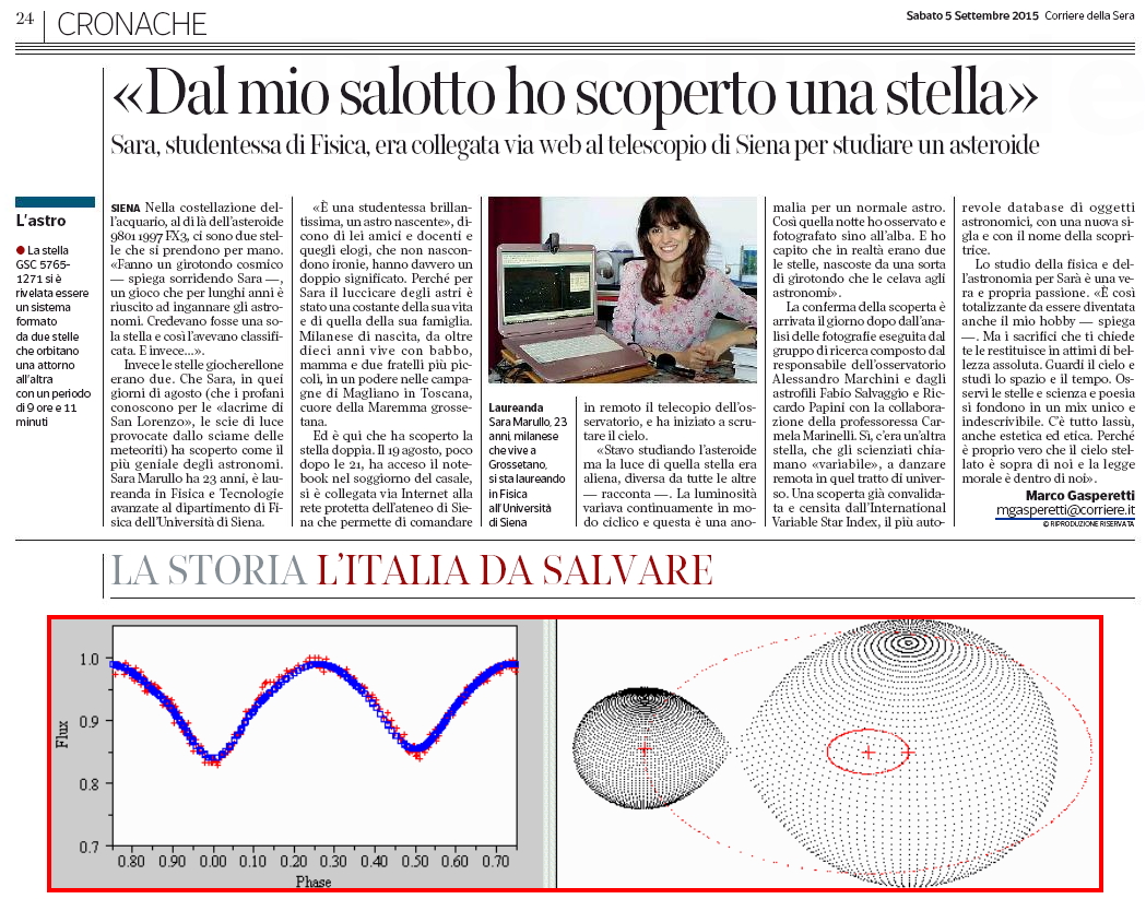
A famous Italian newspaper writes about the binary star discovered by Sara Marullo, and titles: “I discovered a star from my living room”.
Thanks to the automation implemented ten years ago, it has been possible to face the last two years of the Covid-19 pandemic without interrupting teaching, research, and scientific dissemination activities. University students were able to perform remote imaging sessions for their internships, while high school students participated remotely in astrophysics orientation projects.
In April 2020, Leonella Filippa Saya, another student of the course in Physics, although in full pandemic lockdown, was able to finish her university internship and discuss her thesis on the photometric study and 3D modeling of the asteroid (118) Peitho. Her thesis allowed her to appear as the author of an article published in the Minor Planet Bulletin.
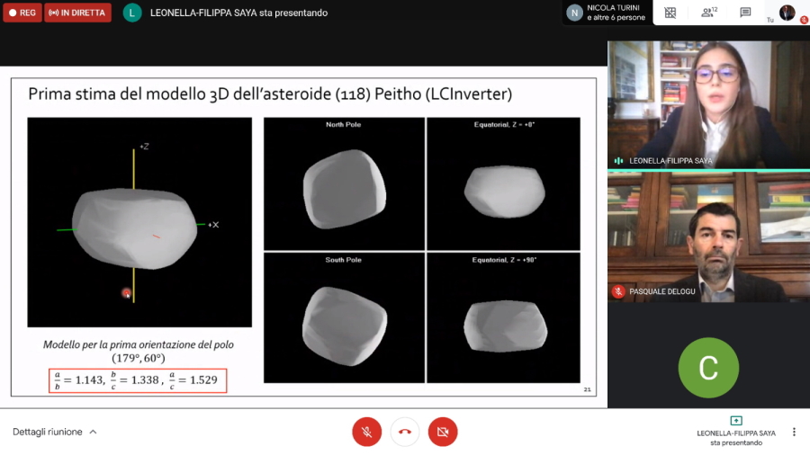
Leonella Filippa Saya discussing her thesis online during the pandemic lockdown.
Many high school students were able to participate remotely in the university guidance course offered by the observatory, entitled "Hunting for ancient photons, astronomy in the digital age".
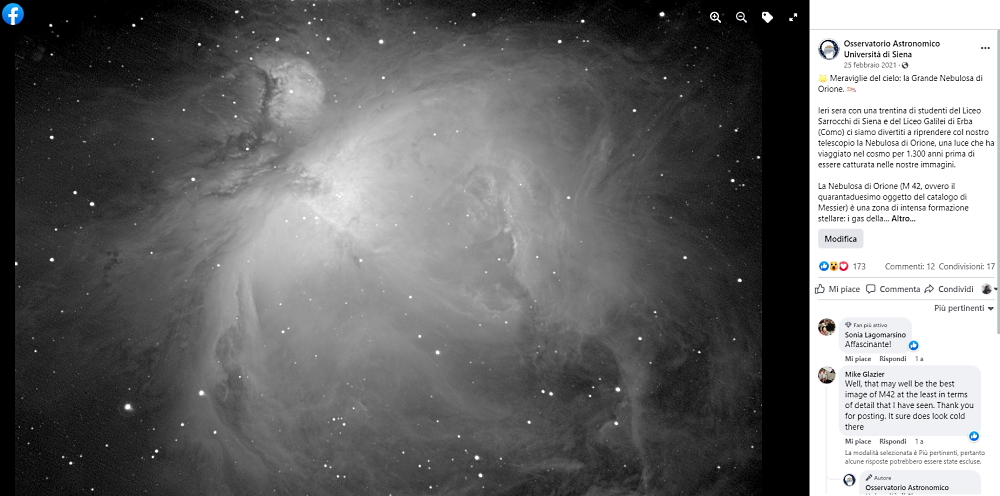
An image of the Great Orion Nebula captured in February 2021 by the students of Liceo “Sarrocchi” in Siena and Liceo "Galilei" in Erba (Como) via remote operation of the telescope from their homes.
Worthy of note is a group of fifteen students from the Liceo “Galilei” in Erba (Como), in Northern Italy, who in June 2020 remotely attended some observing sessions of the asteroid (58) Concordia, and actively participated in data analysis. For their efforts, their names were mentioned in the acknowledgments on a scientific article published in the Minor Planet Bulletin.
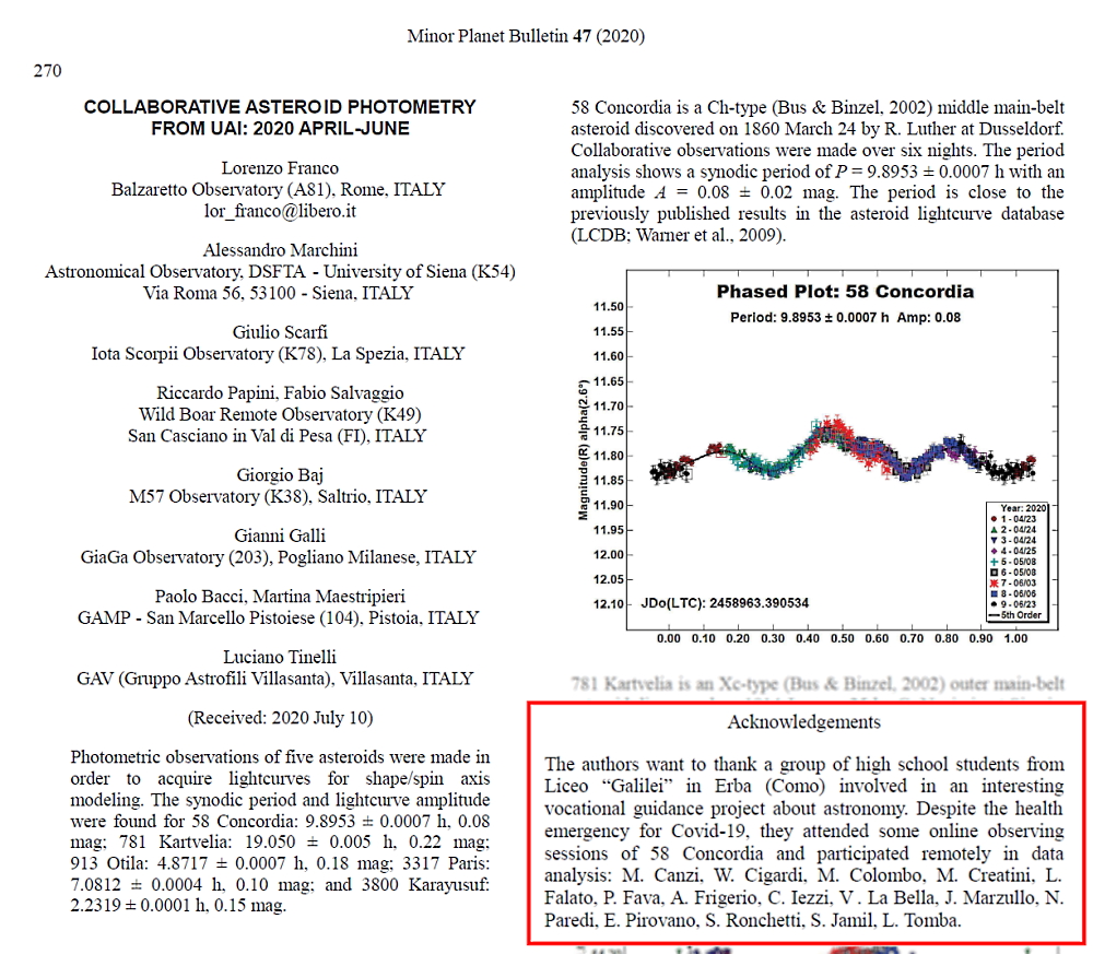
The article published in the Minor Planet Bulletin with the acknowledgments to the students of Liceo "Galilei" in Erba (Como)
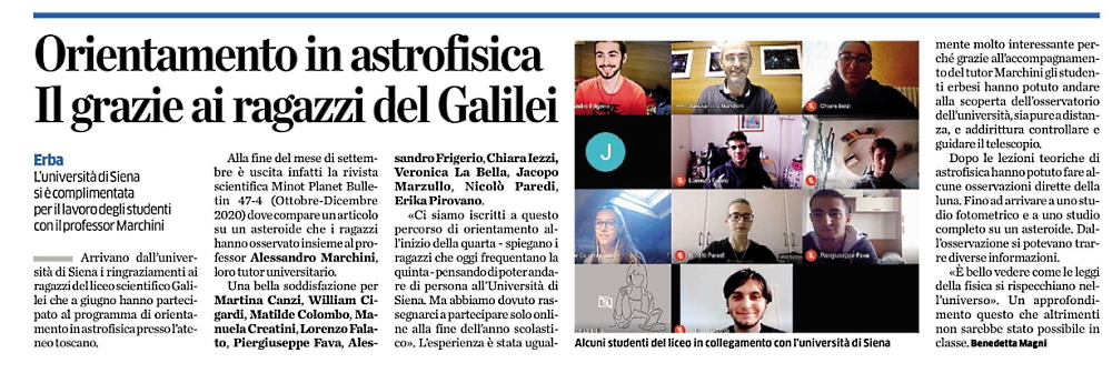
A Como newspaper writes about the guidance project in astrophysics carried out by the students of Liceo "Galilei".
During the entire lockdown period it was also possible to offer many live shows on the observatory's social profiles; these dissemination activities allowed thousands of connected citizens to follow the Observatory’s scientific research, and stimulated them to observe the starry sky from their own windows or gardens. Many of these online initiatives have been organized for particular events such as the arrival of a comet, the close passage of an asteroid, or the super-moon.
One of the most followed live shows, with over 60,000 views on YouTube and Facebook, was the one organized for the spectacular Jupiter-Saturn conjunction on December 21, 2020.
The live show carried out for the Jupiter-Saturn conjunction on December 21, 2020.
While we are fully aware of how much more engaging the physical presence of students and researchers is, since it allows greater empathy between teachers and students or between researchers and the public, the pandemic has forced the astronomical observatory to successfully continue its activities in its purest form, as an instrument: an example of how a serious problem can be transformed into an opportunity thanks to the technology developed over the years.
How to cite: Marchini, A.: An automated Astrophysics lab for everybody: the activities of the Astronomical Observatory of the University of Siena during two years of Covid-19 pandemic., Europlanet Science Congress 2022, Granada, Spain, 18–23 Sep 2022, EPSC2022-1099, https://doi.org/10.5194/epsc2022-1099, 2022.
During 2021 we started a project called Comet Chasers, to work with Primary schools in South Wales, bringing astronomy-related activities into the classroom to teach core skills.
During the period of the project (on 10 June 2021) there was a partial solar eclipse (around 22% in the area), so activities around that event were also included.
Obviously, the ideal scenario was that students would be able to view the full duration of the eclipse using a range of safe/specialist equipment, making and logging their observations for analysis later. Planned observations included using various filters (white light, CaK and Ha) to see different solar features; direct viewing through solar glasses; and indirect viewing through projection with Keplerian Sunspotters.
With a clear sky it would also be possible to use the Sunspotters for activities measuring the rotation of the Earth – with some nice maths involved.
BUT, Wales is not renowned for its good weather, particularly when something as great as a solar eclipse is happening! So backup activities were planned.
The availability of live streams from across the eclipse path was a huge advantage, so it was planned to stream those into the classroom. But just watching a solar eclipse develop over a few hours might not hold the attention of the 10-year-olds in the class, and it did not include much opportunity for learning either. So a varied programme was developed, starting with some of the science of eclipses, with appropriate hands-on activities, then using the functionality in Stellarium Web to simulate the eclipse from any location, and to view at higher speed. Students would simulate what would they be seeing if they were outside and the sky was clear. In addition, they could simulate the view from the locations of the live streams – choosing a location, changing Stellarium settings, matching the simulation with what they were seeing on the live stream and investigating what would happen next/or had just happened. It would also be a fun activity for them to simulate what maybe a relative would see from their location somewhere else….
The day before the eclipse was gloriously sunny, the day of the eclipse was…. cloudy.
But the event was still a success. To quote a student asked about what was most interesting from the Comet Chasers project: ’I found the solar eclipse most interesting when we were able to see it even though our luck was terrible because it was cloudy and rainy.’
We will present how the different activities worked in practice, more feedback from students and their teacher, and what we learnt that could be useful for other projects wishing to use mixed approaches for live events.
Acknowledgements
The Comet Chasers project was administered by Techniquest with initial funding from a Science and Technology Facilities Council SPARKS Award. Access to the telescope facilities in the Las Cumbres Observatory network is provided through the support of the Faulkes Telescope Project.
It is now delivered by a partnership of professional and amateur astronomers, the Open Uiniversity and Cardiff University, working closely with educators.
https://www.cometchasers.org/
https://www.techniquest.org/
https://www.ukri.org/councils/stfc/
https://lco.global/about/
http://www.faulkes-telescope.com/
https://stellarium-web.org/
How to cite: Usher, H. and Vaughan, S.: Using Live Feeds in the Classroom: A case study from a partial solar eclipse in cloudy Wales, Europlanet Science Congress 2022, Granada, Spain, 18–23 Sep 2022, EPSC2022-1240, https://doi.org/10.5194/epsc2022-1240, 2022.
What are the notable forthcoming astronomical events for “the person in the street”? We present a brief overview of notable eclipses, appulses, and other groupings involving the Moon and the naked-eye planets. We’ll also make use of some of our other databases to answer questions such as: what is the biggest solar eclipse in terms of population coverage?
How to cite: Jones, G.: Coming soon to a sky near you: notable naked-eye astronomical events 2022–2040, Europlanet Science Congress 2022, Granada, Spain, 18–23 Sep 2022, EPSC2022-1253, https://doi.org/10.5194/epsc2022-1253, 2022.
ODAA5 | Tools, resources and opportunities for education initiatives in planetary science and astronomy
Introduction: The ESA SPICE Service (ESS) based at the European Space and Astronomy Center (EASC) provides ESAs Solar System Exploration missions ancillary data and geometry information to the science community and to the science ground segments in the shape of SPICE data. Most of this data is three-dimensional, and its interpretation and visualization is one of the challenges faced by the ground segments that operate the spacecrafts and the scientists that study its data. Science Observations and contextual Data analysis of Planetary missions can be naturally accommodated into 3D visualizations. Virtual Reality (VR) brings an unprecedented level of interaction possible with these visualizations, and emerging VR platforms such as Oculus VR, Google Cardboard or Samsung Gear VR are making these technologies accessible to the wide public. VR might become in the near future, not only a tool for outreach and data visualization, but also a key part for spacecraft science operators, becoming a key element of the ground segments.
The ESA SPICE Service: The ESA SPICE Service (ESS) leads the SPICE operations for ESA missions. The group generates the SPICE Kernel Datasets (SKDs) for missions in development (JUICE, ExoMars 2022, Hera, Comet-Interceptor, and EnVision), missions in operations (Mars Express, ExoMars 2016, BepiColombo, and Solar Orbiter) and legacy missions (Venus Express, Rosetta and SMART-1). ESS is also responsible for the generation of SPICE Kernels for INTEGRAL. Moreover, ESS provides SPICE support Kernels for Gaia and James Webb Space Telescope. ESS also provides tools for the exploitation of the SPICE Kernels, consultancy and support to the Science Ground Segments of the planetary missions, the Instrument Teams and the science community. The access point for the ESS activities, data and latest news can be found at the following site https://www.cosmos.esa.int/web/spice. ESS works in partnership with NAIF.
Virtual Reality Applications: Examples of applications of these technologies in operations are already available: the Mars rovers, especially Curiosity have embraced VR and Augmented Reality techniques (some applications are publicly available such as (Access Mars). New mission concepts such as recently selected Dragonfly (a NASA rotorcraft lander for Titan) have already started to develop operation concepts based on VR. Another example of a successful VR application is ESASky [2]. ESASky is a science driven discovery portal developed at ESAC providing full access to the entire sky as observed with Space astronomy missions that has VR extensions and capabilities.
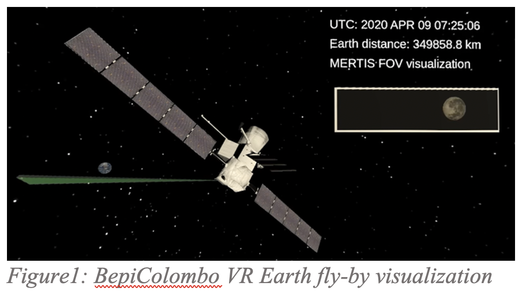
VR for Solar System Exploration: This contribution aims to describe the first steps of delivering advanced functionalities for VR tools created to access Solar System geometry, with particular emphasis on visualization of the science observations carried out by the ESA Planetary fleet on the Solar System (Mars Express, ExoMars2016, BepiColombo, Solar-Orbiter, Rosetta, SMART-1, JUICE, etc.). The functionalities will also include advanced functionalities for navigation and data selection in a VR space through peripherals like Oculus Touch.
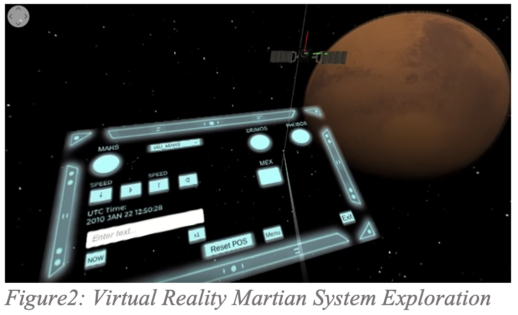
References: [1] Acton C. (1996) Planet. And Space Sci., 44, 65-70. [2] Merin, B. et al., (2015) ESA Sky: a new Astronomy Multi-Mission Interface.
How to cite: Escalante Lopez, A., Valles, R., and Arviset, C.: Solar System Exploration with Virtual Reality, Europlanet Science Congress 2022, Granada, Spain, 18–23 Sep 2022, EPSC2022-9, https://doi.org/10.5194/epsc2022-9, 2022.
Introducing a presentation about the landing sites of Mars landers, and the places on Earth having corresponding coordinates. The presentation is free to use for education and outreach purposes under Creative Commons BY-NC-ND 4.0 license.

How to cite: Kahanpää, H.: Where on Earth are the Mars landers?, Europlanet Science Congress 2022, Granada, Spain, 18–23 Sep 2022, EPSC2022-81, https://doi.org/10.5194/epsc2022-81, 2022.
We will present the opportunities of an ERASMUS+ strategic partnership KA2 funding schemes which we used to support (not only) early career researchers in astronomy. ERASMUS+ is a general funding scheme and we describe here one particular project funding education and international partnerhsip of institutions in astronomical research. Our first Erasmus program (2017-2020) was enabling mobilities of early career researchers between Spanish, Czech and Slovak institutes. The mobilities helped young researchers to gain experience with the modern instrumentation at Observatorio Roque de Los Muchachos at La Palma, Spain. Our program helped several young researchers to obtain tenure track position in astronomical research. We also obtained a continuation of the ERASMUS+ program for another period (2020-2023) which focuses on the development of careers of young researchers and helping them to become future faculty leaders. Furthermore, within the program we performed educational activites for children of various ages. This contribution will describe our programs and its aims and results. We will also share our experience with the application process and with the ERASMUS+ program itself. We will describe the opportunities the ERASMUS+ program is offering for the education in an astronomical research for non-university research institutions.
How to cite: Kabath, P., Jones, D., Garcia Rojas, J., Toth, J., Jakubik, M., Janik, J., and Hanus, J.: Per Aspera ad Astra Simul - ERASMUS+ program supporting mobilities ofyoung astronomers from Spain, Czechia and Slovakia, Europlanet Science Congress 2022, Granada, Spain, 18–23 Sep 2022, EPSC2022-314, https://doi.org/10.5194/epsc2022-314, 2022.
The UK is currently playing a key role in the development of Mars Exploration, with scientists and engineers working on many current and upcoming missions such as the European Space Agency’s Mars Express satellite (2003 – present) and the upcoming Rosalind Franklin Rover (launch TBD). The camera onboard the Rosalind Franklin Rover was designed, built and tested at the Mullard Space Science Laboratory, part of University College London, in Surrey, England. The rover was also assembled at Airbus in Stevenage. These facts are not well known to the public in the UK, and our public engagement project, Eyes on Mars, aims to increase awareness of UK’s involvement in progressing Mars science and with this, promote STEM education in UK. We received funding from the Science and Technology Facilities Council’s Public Engagement Sparks Award and the Royal Astronomical Society education and outreach grant.
To accomplish this, Eyes on Mars has two main foci – a social media campaign and providing resources to be used in classrooms, youth groups and at home. The social media campaign will showcase short and informal snippets of information that highlights Mars facts and various space careers. It will also include interviews of diverse individuals from across Europe that are in the space sector, specifically, highlighting their paths into STEM careers.
Furthermore, Eyes on Mars has put together a selection of free resources that are available to download or given to participating schools to carry out science curriculum activities in class. We have provided various education videos, worksheets and activity plans, including making your own filter wheel similar to the filter wheel onboard the Rosalind Franklin Rover. All materials for this craft activity are provided by the Eyes on Mars team, and are sent out to schools or groups across the UK.
Having both come from state-schools in the UK, and not being in the ‘top-set’ for science at school, Catherine Regan and Priya Patel are now PhD students in planetary physics, researching Mars. Both have been told at some point during their education that they weren’t “clever enough” for a career in science, and are now both working on space missions with NASA and the European Space Agency. We want to use Eyes on Mars to be role models for those that may not think they can succeed in science, and to highlight the different possibilities there are for a career in space, especially in the UK.
How to cite: Regan, C. and Patel, P.: Eyes on Mars - Increasing Awareness of UK based Mars Exploration, Europlanet Science Congress 2022, Granada, Spain, 18–23 Sep 2022, EPSC2022-515, https://doi.org/10.5194/epsc2022-515, 2022.
Since the first decade of the 21st century, UNESCO, the European Commission, the OECD, in addition to several other international organizations, have shown great concern regarding the growing disinterest of young people in scientific areas, thus compromising the future of scientific careers (UNESCO, 1999; NRC, 1996; Report, 2007; Rocard, et al., 2007; European Commission, 2008). The speed with which the contemporary world changes requires the School to reformulate paradigms and practices, in order to respond to the challenges and needs of our times. In this context, it is urgent to promote interdisciplinary strategies, capable of developing research and critical thinking skills, and of preparing students for the demands of contemporary society. But how should we operationalize these measures for real?
The use of Astronomy in Education, considering the fascination that this area of knowledge raises and the availability of natural resources, in addition to its interdisciplinary nature, presents itself as an important tool for Education. The fact that astronomy is present in our daily lives and brings together a huge variety of knowledge from different disciplinary areas (from Science to Humanities, passing through Art) opens the way to the development of a myriad of activities and educational projects aligned not only with the curricula of different disciplines, but also mobilizing several areas of knowledge and multiple scientific competences and soft-skills. It is therefore important to bring to the field good practices about hands-on and mind-on astronomy activities.
The good practices that I will share are the result of my own experience with Portuguese students, ranging from simple experiences using traditional school supplies, or materials that can be produced by the students themselves, to experiences using robotic telescopes, in which the student puts himself in the shoes of true scientists, to initiatives that promote scientific literacy in the community where the school is located.
Activities such as the Eratosthenes Project, for the determination of the Earth's perimeter, are an excellent example of an activity that, without involving costs, shows the power of human genius mobilizing knowledge of Geography, Physics, Mathematics, History, Arts, of ICT. Students are challenged to determine the size of the Earth just with a stick and knowledge. More than a challenge for the students, it is a challenge for the School in the way it will have to organize itself in a project that involves several disciplines. It will be the advent of a School that needs to reinvent itself, using greater plasticity and interdisciplinarity. The use of sunlight, and the shadows produced by it, can provide a whole variety of experiences that essentially involve concepts of Physics, Mathematics and Geography from the apparent movement of the Sun. The determination of the solar diameter by projection of sunlight through a pinhole using a DiY device that allows varying the distance from the pinhole to the target allows working mathematical concepts associated with the representation and graphical analysis of functions with an experimental basis, such as working with the concept of errors experiments and a way to correct them, something fundamental in Physics and Chemistry.
In addition to these experimental activities, School has an obligation to break down its walls and get closer to the community in which it operates, promoting events open to the public in which the scientific literacy of these communities is enriched. At Escola Secundária Marques Castilho (Águeda, Portugal) we promote an activity called “from my school I see the Universe”. Students from a secondary school class were mobilized to carry out a small project which resulted in an exhibition that was open to the public at the Municipal Library of Águeda. This activity was further enhanced with a Lecture with scientist (Dr. João Fernandes of University of Coimbra) and astronomical observation sessions with portable telescopes, both open to the community. This is another way of changing School, bringing it closer to the community and providing other forms of public service.
But School through Astronomy also enables a new approach: Teaching Science by doing Science: An example of this are the initiatives we have participated in, such as the use of robotic telescopes in real time, in the classroom. Access to the telescope constellations of the LCO/Faulkes Telescope Project network and the Liverpool Telescope of the National Schools' Observatory, or the “EU-Hands on Universe” radiotelescope network, allows a very high level of motivational and scientific experience to students. In 2016 I worked with a group of students, at a Science Club, studying the supernova SN2016adj in Centaurus A. With the collaboration of the Faulkes Telescope Project, we followed the depletion of the supernova over time, recording, measuring magnitudes and tracing light curves using SalsaJ and Excel spreadsheets. It was an unforgettable experience in which the students felt their self-esteem rise, feeling that they were discovering something still unknown. It was an unforgettable experience in which the students felt their self-esteem rise, feeling that they were discovering something still unknown. This feeling is important to bring to school. Something similar happens to students who participate in asteroid research campaigns.
A simple observation session with robotic telescopes, in real time, can represent an experience of enormous interdisciplinarity, working on concepts of Chemistry related to the electronic transitions of atomic hydrogen (HAlpha), to the structures of vision for the perception of color in Physics am Biology fields, time zones against the location of the telescope in use for Geography, CCD technology, among many other subjects that can be explored.
NUCLIO, together with several other partners, are developing activities for schools in Projects such as LaSciL, CliC-PoLiT, Open Teach, Design-CT, and others projects with teacher training to use Space and Astronomy, associating teaching methodologies by Inquiry and Project Based Learning, for schools interested in embracing new approaches that point the way to the future.
How to cite: Folhas, A.: Astronomy: a way to interdisciplinarity in Science Teaching, Europlanet Science Congress 2022, Granada, Spain, 18–23 Sep 2022, EPSC2022-1154, https://doi.org/10.5194/epsc2022-1154, 2022.
CC is now expanding to provide resources to meet the needs of CfW and the Welsh language. CfW was first implemented in September 2021, shifting the educational focus from content-based learning to skills-based learning, giving teachers more freedom regarding the contents of their lessons. This brings in novel complications, like the difficulty of preparing educational and stimulating lessons while also including the required skills. CC aims to solve these problems by supplying teachers with a variety of easy-to-follow lesson plans, encompassing a range of required key skills.
As part of CC, students can experience the whole ‘astronomical research process’, from planning when to obtain observations, to requesting the capture of images using the Faulkes Telescope Project (FTP) to access the Las Cumbres Observatory robotic telescope network, to analysing their images and plotting the results. The data are also used by pro-am astronomers to analyse the objects for their own research. CC schools will then be included in any subsequent publications that utilise data obtained by students - an inspiring and exciting opportunity. Over 100 children from 4 primary schools in South Wales were involved in the CC pilot, and 3 of these schools were included on a 2021 ApJ paper, Physical Characterization of Main-belt Comet (248370) 2005 QN173 [1], with another publication under review.
Student feedback:
“It is amazing and cool that our little school in Mid Wales can control a big telescope in Australia from our classroom”.
“Amazing, I can’t explain how cool and inspiring [it is]”.
Teacher feedback:
“We have learnt so much about astronomy. But the activities cover so many other parts of the curriculum too!”
“It has been fantastic. I’ve enjoyed it and the children have absolutely loved it. I wish we had more time each week as there was so much great material.”
Teacher guides, videos and worksheets for students have been produced, explaining the core concepts behind comets, space, light, how to collect data, and how to measure data, in addition to guiding schools through all the processes needed to obtain and analyse images. Web-based tools are being developed to assist in these processes. This exposes pupils to real scientific research and procedures, helping to nurture a deeper interest and understanding of current science.
All resources and tools will be available in Welsh to expand CC to involve Welsh language schools throughout the country. Welsh language STEM projects are uncommon, which can lead to a decrease in STEM engagement in this population. Providing Welsh language resources gives new and exciting opportunities for students in what are often under-performing schools [2]. Student results in Welsh language schools are marked lower than students in English language schools, suggesting Welsh resources may not be of high enough quality. CC aims to ensure that our resources put Welsh and English language schools on a level playing field, giving equal opportunities and successes in the project for all schools.
The main aim of CC for the future is expansion, both geographically and in participant ages. This will include schools outside of Wales, to share our knowledge, tools, and materials with other partners. Translation of resources into languages other than Welsh or English will be encouraged. CC also intends to involve older school children (ages 14-18) where more emphasis can be put on the science in addition to conducing more complex data analysis.
[1] Hsieh, H.H., et al., 2021. Physical Characterization of Main-Belt Comet (248370) 2005 QN173, ApJ. 992(1).
[2] Johnes, G. (2020) ‘Medium Efficiency: Comparing Inputs and Outputs by Language of Instruction in Secondary Schools in Wales’, Wales Journal of Education. 22(2) :52-66.
How to cite: Stoddard-Jones, C., Roche, P., Usher, H., Miles, R., Angel, T., Wooding, B., and Wooding, S.: Chasing Comets in the Land of Dragons/Chwilotwyr Comedau yn Wlad y Dreigiau: Pro-Am-Schools collaboration to engage students in STEM in Wales., Europlanet Science Congress 2022, Granada, Spain, 18–23 Sep 2022, EPSC2022-1172, https://doi.org/10.5194/epsc2022-1172, 2022.

The pandemic crisis has reshaped the landscape of formal education worldwide and caused critical challenges for teachers. The most encountered issues can be listed as follows; keeping students motivated to actively engage them in a virtual classroom, ensuring the learning outcomes of the lessons, and adapting their educational practice in a more inclusive and personalised approach to address different types of learners.
In order to address the aforementioned challenges faced by teachers in the school environment, the Erasmus+ project LaSciL brings together schools in Europe, educational research institutions, outreach groups, and Large Scientific infrastructures in Physics. These include robotic telescopes and an astronomical observatory with a group of operators of large scientific infrastructures, education, and outreach specialists, together with school education experts. The aim is to enhance teachers’ digital competence by supporting high-quality science teaching in the classroom from a distance as well as supporting a long-term organisational restructuring of schools.
LaSciL empowers and supports teachers to become more literate in using high-quality digital educational tools. In this framework, teachers shall be enabled to a) create their own opensource educational resources for their students’ distance learning; b) manage large numbers of students in an online environment by keeping them motivated to participate, c) maintain and enhance their science motivation and d) personalise their teaching practices tailored to the needs of their students. To achieve that, LaSciL demonstrates innovative ways to involve teachers and students in eScience by sharing and exploiting the collective power of highquality digital resources (research facilities, scientific instruments, advanced ICT (Information and Communication Technology) tools, simulation and visualisation applications, and scientific databases). The LaSciL project provides teachers with cutting-edge, curriculum-tailored educational scenarios that can be used, reused, and adapted to their needs, as well as act as a source of inspiration for the design of their own open educational content through active educational methodologies such as Inquiry based learning and Project based learning.
Through careful monitoring and assessment of the teacher training and implementation with students, LaSciL develops a series of best practices and devises a roadmap both for supporting science teachers and proposing a new organisational framework to enable close collaborations between schools and research infrastructures. This connection demonstrates effective ways of involving a broader set of actors in the use of research infrastructures by
developing a framework of actions that will attract young people to science and pool talent to scientific careers.
LaSciL presents both a short-term and a long-term vision. In the short term, we a) support the development of key teacher ICT competencies and digital readiness; b) produce a series of high-quality digital tools and educational resources ready to be implemented in the classroom and c) facilitate instruction in the pandemic era, maintaining and enhancing students’ science motivation and fascination without compromising the curriculum. In the long term, LaSciL envisions a new organisational framework for the collaboration between schools and research infrastructures.
LaSciL promotes a culture of cooperation between research infrastructures, by spreading good practices among outreach groups of large-scale research infrastructures, encouraging them to develop their activities in complementary ways and to optimise their use by demonstrating how e-infrastructures, such as robotic telescopes, could support the vision of the science classroom of tomorrow.
How to cite: Özdemir, S., Lewis, F., Roberts, S., Doran, R., Rojas, G., Folhas, A., Panagopoulou, M., Chaniotakis, E., Evangelopoulos, P., Charmandaris, V., Groemer, G., and Albrecht, K.: Large Scientific Infrastructures enriching online and digital Learning: LaSciL, Europlanet Science Congress 2022, Granada, Spain, 18–23 Sep 2022, EPSC2022-1270, https://doi.org/10.5194/epsc2022-1270, 2022.
ODAA6 | Open planetary science for effective knowledge co-creation and dissemination
Abstract
The Gaia@home project is designed to give scientists another layer of freedom. The project makes possible to perform computations which demand a lot of CPU time – reducing the computational workload and opening up opportunities for heavy processing operations on volunteers computers.Gaia@home allows to create a huge number of small jobs (Gaia data + code), send them to the BOINC platform and collect the results for further analysis.Enjoy Gaia@home either if you are a scientist looking for CPU resources or a volunteer willing to contribute to citizen science.

Figure 1. Gaia@home logo.
Are you a scientist? Gaia@home can speed up your science!
- Step 1: Visit https://web.gaiaathome.eu/login and create an account
- Step 2: Prepare the code used for your calculations following some BOINC rules. Instructions are provided in our site. The code can compute any scientific problem which relies on the Gaia archive data, but also feel free to attach your own data.
- Step 3: Create a new task. Every task consists of the executable file, compiled according to BOINC guidance (step 2), auxiliary files (e.g. additional input file needed for any job) and a prescription on how to split Gaia archive into a series of parallel, independent jobs. Every BOINC job gets these files, and one portion of the data from the Gaia archive.
- Step 4: Your task starts running and you will be notified when a number of jobs on the BOINC platform have been completed.
- Step 5: You will be periodically notified by email about the status of your calculations. Finally, you will be notified when the task is completed and you are ready to download your results!

Figure 2. Screenshot of Gaia@home showing the current available computation resources from volunteers.
Would you like to contribute to citizen science? Volunteer your free resources!
- Step 1: Visit http://www.gaiaathome.eu and press on Volunteer now!
- Step 2: Create an account in BOINC
- Step 3: Install BOINC app in your device, and start contributing to science!
Acknowledgements
This work has received funding from European Space Agence under the polish industry incentive scheme - GAVIP-GridComputing (4000120180/17/NL/CBi).
TSR acknowledges funding from the NEO-MAPP project (H2020-EU-2-1-6/870377). This work was (partially) funded by the Spanish MICIN/AEI/10.13039/ the Institute of Cosmos Sciences University of Barcelona (ICCUB, Unidad de Excelencia ‘María de Maeztu’) through grant CEX2019-000918-M.
How to cite: Bartczak, P., Santana-Ros, T., Hypki, A., Langner, K., and Dudziński, G.: Gaia@home: Combining Gaia catalogue with the power of volunteer computing, Europlanet Science Congress 2022, Granada, Spain, 18–23 Sep 2022, EPSC2022-659, https://doi.org/10.5194/epsc2022-659, 2022.
In August 2020, Europlanet launched the Mentorship platform with the aim to support early career researchers. Two years after launch we are using a survey to gather feedback from mentors and mentees, and we are also following up with participants informally through chats and e-mails. The feedback so far has been positive and points to the effectiveness and the need of the programme to support the paths of early career researchers. We will present the Europlanet mentorship programme and the case study of the Romanian/Brazil collaboration that resulted from the mentor's work with two mentees. Europlanet 2024 RI has received funding from the European Union's Horizon 2020 research and innovation programme under grant agreement No 871149.
How to cite: Stonkute, E., Tautvaisiene, G., Heward, A., and Mikolaitis, S.: Europlanet Mentorship programme: opportunities for sharing the knowledge, Europlanet Science Congress 2022, Granada, Spain, 18–23 Sep 2022, EPSC2022-808, https://doi.org/10.5194/epsc2022-808, 2022.
Abstract
Objectives for Phase II of NASA’s Artemis Program include establishment of lunar surface infrastructure to support a sustainable, long-term human presence on the Moon. Terrestrially, awareness of climate impacts from cement and concrete production has led to renewed interest in traditional building materials using earthen and pozzolanic binders with locally sourced aggregates [1, 2, 3]. In remote, austere and resource-constrained environments, use of site-sourced materials is often an economic necessity in addition to being valuable for local autonomy and self-sufficiency. This study evaluates modifications to ASTM cement mortar testing methods, incorporating details from European standards for earthen plasters and lime-based mortars. Development of consistent, simplified methods for evaluating in-situ materials will be essential not only for meeting future climate goals and sustainable construction needs, but also for conducting autonomous robotic manipulation and evaluation of regolith construction materials.
Introduction:
Recent studies of in-situ derived simulant-based building materials for construction on the surface of the Moon and Mars have drawn on traditional building techniques and their renewed use in sustainable construction [4, 5]. Humans have experience spanning millennia building with site soils and locally-derived mineral materials. In addition to examples found at archaeological sites and historic buildings surviving to the present, some earthen building traditions (adobe, mud plastering) continue to be practiced to this day [6, 7], while others are seeing broader adoption in innovative construction techniques using 3D printing [8, 9].
In this study, a selection of these formulations were adapted for use with planetary analog site soils to assess the suitability of these methods in evaluating potential regolith construction materials for in-situ construction on planetary surfaces [10]. These studies focused on curing and compressive strength testing of preliminary mix formulations using small mortar specimens in ambient conditions.
Materials Testing Methods for Mortars and Extruded Materials:
Basic evaluations of soil-based building materials begin with particle size distribution and compressive strength. In North America, these assessments are often conducted following ASTM C-109, “Standard Test Method for Compressive Strength of Hydraulic Cement Mortars (Using 2-in. or [50 mm] Cube Specimens)” [11] in conjunction with ASTM C-144 (Standard Specification for Aggregate for Masonry Mortar) [12] and ASTM C-136 (Standard Test Method for Sieve Analysis of Fine and Coarse Aggregates) [13]. Key details of ASTM C109 requiring submersion of specimens in water during curing preclude its use with non-cementitious binders. Techniques used in evaluation of traditional clay plasters (DIN 18947) [14], lime mortars (EN 1015) [15] and pozzolanic materials were adapted here for use with specimens prepared from construction site mixes using local soils, industrial byproducts, organic additives and bagged materials from masonry and ceramic suppliers.
Key Findings & Opportunities:
Drawing upon European standards for traditional building materials and sustainable building products to modify ASTM methods can enable study of site-sourced, minimally-processed non-cement materials for terrestrial and planetary surface construction. Experience in refining these methods alongside researchers in sustainable construction demonstrates that: 1) tradespeople and craft builders in traditional construction have a valuable contribution to offer to the study of materials for in-situ construction on planetary surfaces, and 2) that development of consistent, simplified methods for use in preliminary testing of varied simulant and in-situ soil formulations for construction may enable opportunities for interdisciplinary collaboration with mutual benefits for terrestrial sustainable building and in-situ regolith construction on the Moon and Mars.
References:
[1] Delinière, R., Aubert, J. E., Rojat, F., & Gasc-Barbier, M. (2014). Physical, mineralogical and mechanical characterization of ready-mixed clay plaster. Building and Environment, 80, 11-17.
[2] MacDougall, C., & Vardy, S. (2014). Mechanical performance of lime-cement mortar for straw-bale construction. Journal of Green Building, 9(3), 100-115.
[3] Seitz, S., Haynes, R. & Glass, B. “Playing With DIRT: Building the Framework for a Comprehensive Materials Database.” ASCE Earth & Space 2022 Conference, Denver, Colorado.
[4] Rosa, I., Coto, A., Allende, M. I., Lepech, M. D., & Loftus, D. J. (2021). Designing Biopolymer-Bound Regolith Composites for Maximum Compressive Strength. Earth and Space 2021, 200-214.
[5] Karl, D., Duminy, T., Lima, P., Kamutzki, F., Gili, A., Zocca, A., Günster, J. and Gurlo, A., 2020. Clay in situ resource utilization with Mars global simulant slurries for additive manufacturing and traditional shaping of unfired green bodies. Acta Astronautica, 174, pp.241-253.
[6] Taylor, B., Vardy, S., & MacDougall, C. (2006). Compressive strength testing of earthen plasters for straw bale wall application. In Advances in Engineering Structures, Mechanics & Construction(pp. 175-183). Springer, Dordrecht.
[7] Faria, Paulina, and Vitor Silva. "Natural hydraulic lime mortars: influence of the aggregates." Historic Mortars. Springer, Cham, 2019. 185-199.
[8] Mueller, R. et al. (2019). “NASA Centennial Challenge: 3D Printed Habitat, Phase 3 Final Results.” 70th International Astronautical Congress (IAC), October 21-25, 2019, Washington, DC.
[9] Biggerstaff, A., Fuller, G., Lepech, M., & Loftus, D. (2021). Determining the yield stress of a Biopolymer-bound Soil Composite for extrusion-based 3D printing applications. Construction and Building Materials, 305, 124730.
[10] Seitz, S. (2019). “Building Materials for the Moon & Mars: Mortar Testing Methods for Regolith.” ASCE EMI – MS99, Pasadena, CA.
[11] ASTM (2021). ASTM C109 - Standard Test Method for Compressive Strength of Hydraulic Cement Mortars (Using 2-in. or (50-mm) Cube Specimens).
[12] ASTM (2021). ASTM C136 - Standard Test Method for Sieve Analysis of Fine and Coarse Aggregates. West Conshohocken, Pennsylvania: ASTM International.
[13] ASTM (2021). ASTM C144 - Standard Specification for Aggregate for Masonry Mortar. West Conshohocken, Pennsylvania: ASTM International.
[14] Deutsches Institut Fur Normung E.V. (2018). “DIN 18947 - Earth plasters – Requirements, test and labelling.” https://dx.doi.org/10.31030/2897115.
[15] EN 1015-11:1999; Methods of Test for Mortar for Masonry—Part 11: Determination of Flexural and Compressive Strength of Hardened Mortar. BSI.
How to cite: Seitz, S., MacDougall, C., and Glass, B.: Enabling Evaluation of In-Situ Regolith-Based Construction Materials with Modified Methods for Testing Compressive Strength of Non-Cement Mortar Specimens Using Simulants & Analog Site Soils, Europlanet Science Congress 2022, Granada, Spain, 18–23 Sep 2022, EPSC2022-1092, https://doi.org/10.5194/epsc2022-1092, 2022.
Although the apparition of the Open Science policy at European level in 2018 is expected to trigger a sharp increase in scientific activity, is it a challenge to the community. Most notably, data related to publications or produced during programmes funded on public money (such as H2020 / Horizon Europe, and national programmes) now need to be made accessible according to FAIR principles. Beyond easy availability of published articles, the principle of open access to the data, may result in an increase in spending that would mainly benefit private editors.
However, mature solutions to this problem exist in the academic world, which are not only economical and rewarding, but also accessible to small research teams. These solutions also have applications to citizen science and pro-amateur projects.
The Virtual Observatory. VESPA (Virtual European Solar and Planetary Access) has focused for 10 years on adapting Virtual Observatory (VO) techniques to handle Planetary Science data [1] [2]. The objective of this activity is to build a contributory data distribution system both to access and publish data with minimum fuss. This system is responsive to the new paradigm of Open Science and FAIR access to the data, and is optimized to publish data with limited resources. VESPA therefore relies on an infrastructure maintained by the astronomical community, and enlarges it to support Planetary Science by publishing additional standards, increasing compliance with other fields (Earth observation, heliophysics, space physics…), and adding new capacities to existing tools.
Data description and access. VESPA uses a standard access protocol called TAP, associated with a metadata vocabulary providing uniform description of datasets in the field (EPN-TAP). At the time of writing EPN-TAP is in the final stage of becoming a Recommendation of the International Virtual Observatory Alliance (IVOA) [3]. Many tools can search data services based on EPN-TAP, in particular the VESPA portal (http://vespa.obspm.fr), generic VO clients, and VO tools which also provide visualisation and processing functions (e.g. TOPCAT, Aladin, CASSIS for tabular data, images, and spectra). Specific access modes (via script, web services, Jupyter notebook, etc) are also available for advance usage. The VESPA portal is intended as a discovery tool that queries all EPN-TAP services together. It provides a convenient way to search archives described with the EPN-TAP metadata vocabulary, to cross-search many databases, and to send selected data products to generic, high-level visualization and processing tools maintained by the astronomy community.
Practical implementation relies on 60+ published data services from 20+ institutes, offering a variety of situations. The recommended method consists in the installation of a data server supporting EPN-TAP, which is available in a Docker container and can easily be deployed anywhere. This only requires permanent web connection and URL for the server, and it takes advantage of a global infrastructure supported by the community (registry of services and VO tools). Generic tutorials are available for easy implementation – in a typical situation, data ingestion only requires a CSV list of data products described by the EPN-TAP parameters, although existing databases can be used to build a data service.
Service publication is granted by simply declaring it in a common registry. The data themselves can be located anywhere, either locally or on public storage facilities such as Zenodo or B2SHARE (where VESPA communities have been declared).
Contributory science. VESPA already distributes archives from pro-amateur collaborations, in particular PVOL for planetary images, but also RadioJove for radio observations of Jupiter (NASA-supervised project). Such archives are very helpful to complement professional surveys by filling gaps at several time scales with observations from multiple locations.
A number of collaborative projects are discussed in the frame of Europlanet 2024 RI (NA2 activity), including: the telescopic network (test server already installed); fireball networks (individually or with a common data distribution facility); observations of comets.
Public availability and easy, structured access to the data obviously have potential applications to teaching and outreach.
Access to derived data and science results. Although observatories and space agencies have open archives, they are usually limited to raw or calibrated products, and do not include science-ready data published in articles. ESA’s Planetary Science Archive as an EPN-TAP interface, as well as several ground-based facilities. Existing repositories of derived data include the ESA Guest Storage Facility (hardly searchable currently) and VizieR catalogue of article tables relevant to Solar System studies (available as an EPN-TAP service).
Support. In the frame of the Europlanet 2024 RI programme at least, the VESPA team gladly provides support to users and potential data providers. This of course is intended to become a community infrastructure and to outlive the Europlanet programmes.
The Europlanet-2024 Research Infrastructure project has received funding from the European Union's Horizon 2020 research and innovation programme under grant agreements No 871149.
[1] Erard et al 2018, Planet. Space Sci. 150, 65-85. 10.1016/j.pss.2017.05.013. ArXiv 1705.09727
[2] Erard et al. 2020, Data Science Journal 19, 22. doi: 10.5334/dsj-2020-022.
[3] https://ivoa.net/documents/EPNTAP/
How to cite: Erard, S. and the VESPA team: Open Science policy and Solar System data: contribution from Europlanet/VESPA, Europlanet Science Congress 2022, Granada, Spain, 18–23 Sep 2022, EPSC2022-1116, https://doi.org/10.5194/epsc2022-1116, 2022.
The Webb Space Telescope, a worldwide mission proposing exceptional scientific advances, was launched in Kourou on December 25, 2021. For the project Guiana to the Stars, a team of ten researchers from French laboratories involved in the mission - Paris Observatory - PSL, CEA and IAS - with the support of the science outreach association SpaceBus France, took advantage of this opportunity to reach out to citizens and promote science-society dialogue around astronomy.
From December 5 to 22, 2021, our group of scientists crisscrossed French Guiana. They explained the major challenges and expectations related to the launch of the new telescope in space, with the following objectives:
- To introduce people to astronomy and science through playful, interactive, and accessible animations.
- To demonstrate the scientific method and develop critical thinking through a rich program of conferences.
- To testify of the cultural richness and the international aspect of space-related professions.
- To create vocations and promote the place of women in science to fight against their under-representation in this sector.
The Guiana to the Stars tour covered 2,500 kilometers, in 12 cities through 60 events. The team visited schools, markets, villages, social centers, touristic spots, public places, and the Guiana Space Center. All along the route, we planned animations and activities adapted to the audiences encountered:
- For primary through high school students, the team of scientists proposed science workshops around space and astronomy. These workshops were also an opportunity for the students to meet and exchange with astrophysicists, in particular about space-related professions.
- For teachers of all levels, two astronomers of the Observatoire de Paris - PSL provided academic training in astronomy through general courses, activities, and initiations to night sky observations.
- For the public, astrophysicists gave astronomy conferences and led educational activities and night-time observations. These were proposed free of charge in public places, in the afternoon and in the evening, with the support of the mediators of the Canopée des Sciences.
Ambitious and original, this science outreach operation received the support of the President of the Territorial Collectivity of Guyana. It is placed under the high patronage of the French Minister of Overseas Territories and is sponsored by the French Minister Delegate in charge of Citizenship.
The Guiana to the stars project is carried by Alain Doressoundiram, researcher at the Observatoire de Paris - PSL, and Raphaël Peralta, researcher at the CEA and president of the SpaceBus France association. It has received financial and logistical support from the CEA, the Observatoire de Paris - PSL, the SpaceBus France association, the Académie de Guyane, the Canopée des Sciences, the CNES, the Maison pour la Science en Guyane, the French Government, the CNRS, the Université Paris Science et Lettres, the OSUPS, the SF2A, the IAS, the Unistellar company, the Collectivité Territoriale de Guyane and the Main à la Pâte foundation.
The whole program of the tour can be found on: https://www.jwst.fr/la-guyane-vers-les-etoiles/
How to cite: Peralta, R. and Doressoundiram, A.: Guiana to the Stars: science outreach tour for the Webb space telescope launch, Europlanet Science Congress 2022, Granada, Spain, 18–23 Sep 2022, EPSC2022-1182, https://doi.org/10.5194/epsc2022-1182, 2022.