BepiColombo is a joint mission to Mercury between the European Space Agency (ESA) and the Japanese Aerospace Exploration Agency (JAXA), launched in October 2018. It is now near the end of its eight-year-long cruise to the planet, during which it encountered the Earth and Venus, and performed six flybys of Mercury. In early September 2026, the Mercury Transfer Module will have detached from the mission’s two orbiters. At the time of this meeting, the Mercury Planetary Orbiter (MPO) and the Mercury Magnetospheric Orbiter (Mio) are travelling towards Mercury and will together enter orbit about the planet in late November. These two orbiters will separate from each other on 9-10 December. MPO will adjust its orbit until reaching its final science orbit in March 2027. In April 2027, both orbiters will begin their joint comprehensive exploration of planet Mercury and its environment with their extremely capable payload suites. We shall provide an overview of the two orbiters and their instruments, a summary of the mission status, a preview of the remaining plans for the mission, and a broad overview of scientific results to date.

How to cite: Jones, G., Murakami, G., and Besse, S.: BepiColombo on Final Approach: A Mission Update, Europlanet Science Congress 2026, The Hague, The Netherlands, 7–11 Sep 2026, EPSC2026-867, https://doi.org/10.5194/epsc2026-867, 2026.

EPSC2026-867

Download Close

The ESA-JAXA joint mission BepiColombo is still on the track to Mercury and will be inserted into Mercury orbit in November 2026. It completed all flybys by January 2025 and conducted numerous scientific observations. The Mercury Transfer Module will be first separated in September 2026, followed by insertion into Mercury's orbit in November 2026. Subsequently, the Mercury Magnetospheric Orbiter (Mio) will separate in December 2026, deploying its wire antennas and magnetometer masts. Following initial checkout of the spacecraft bus and scientific instruments, along with test observations, the nominal science phase will start in April 2027. The baseline observation plans for Mio faces thermal constraints during the perihelion season and power constraints during the aphelion season, respectively. Operation planning and updating is progressing to address these limitations. In addition, as available communication time is also limited, we are preparing baseline downlink plans. This presentation will report on the latest status of BepiColombo/Mio and its upcoming operation and observation plans.

How to cite: Murakami, G., Jones, G., and Besse, S.: Updated operation and observation plans of BepiColombo/Mio, Europlanet Science Congress 2026, The Hague, The Netherlands, 7–11 Sep 2026, EPSC2026-343, https://doi.org/10.5194/epsc2026-343, 2026.

EPSC2026-343

Download Close

Introduction

The BepiColombo mission will be inserted around Mercury on November 26^th 2026, and scientific operations will start in March 2027, after the separation between Mercury Planetary Orbiter (MPO) and Mercury Magnetospheric Orbiter (MMO) on December. Probing the Hermean Exosphere By Ultraviolet Spectroscopy (PHEBUS), on MPO, is a UV spectrograph measuring the UV exospheric emissions with two main detectors: Extreme UV (EUV) (55-155 nm) and Far UV (FUV) (145 – 315 nm) and two Near UV (NUVs) channels at 404 nm and 422 nm [1,2]. A combination of a rotating primary mirror and baffle allows changing the pointing direction of PHEBUS field of view. The line of sight changes with the scanner position along a cone with a half-angle of 80° and centered on the Y axis of the spacecraft.

The emissions of H (121.6 nm), He (58.3 nm), Ca (422 nm), and Mg (285.3 nm), observed either by Mariner 10 or MESSENGER as well as the dayside surface, have been observed by PHEBUS during the flybys of Mercury by BepiColombo [3,4,5,6]. More systematic observations of the exosphere of Mercury will be performed during the orbital phase to study its variations. These observations will help to understand the origin of the different species in the exosphere of Mercury, and its relation to the surface and the plasma environment.

We present here the planification of the observations for the first two months during the Medium Term Plans 1 and 2 (MTP 1 and MTP 2) from March 14^th 2027 to May 9^th 2027.

Planification during Medium Term Plans 1 and 2

The orbit plane of MPO through Mercury year is represented on Fig. 1

Fig. 1 The evolution of the orbit plane of MPO through one Mercury year. The observations of PHEBUS are limited to approximatively the MPO orbit plane (red line) and then restricted in local time, depending on the TAA of Mercury.

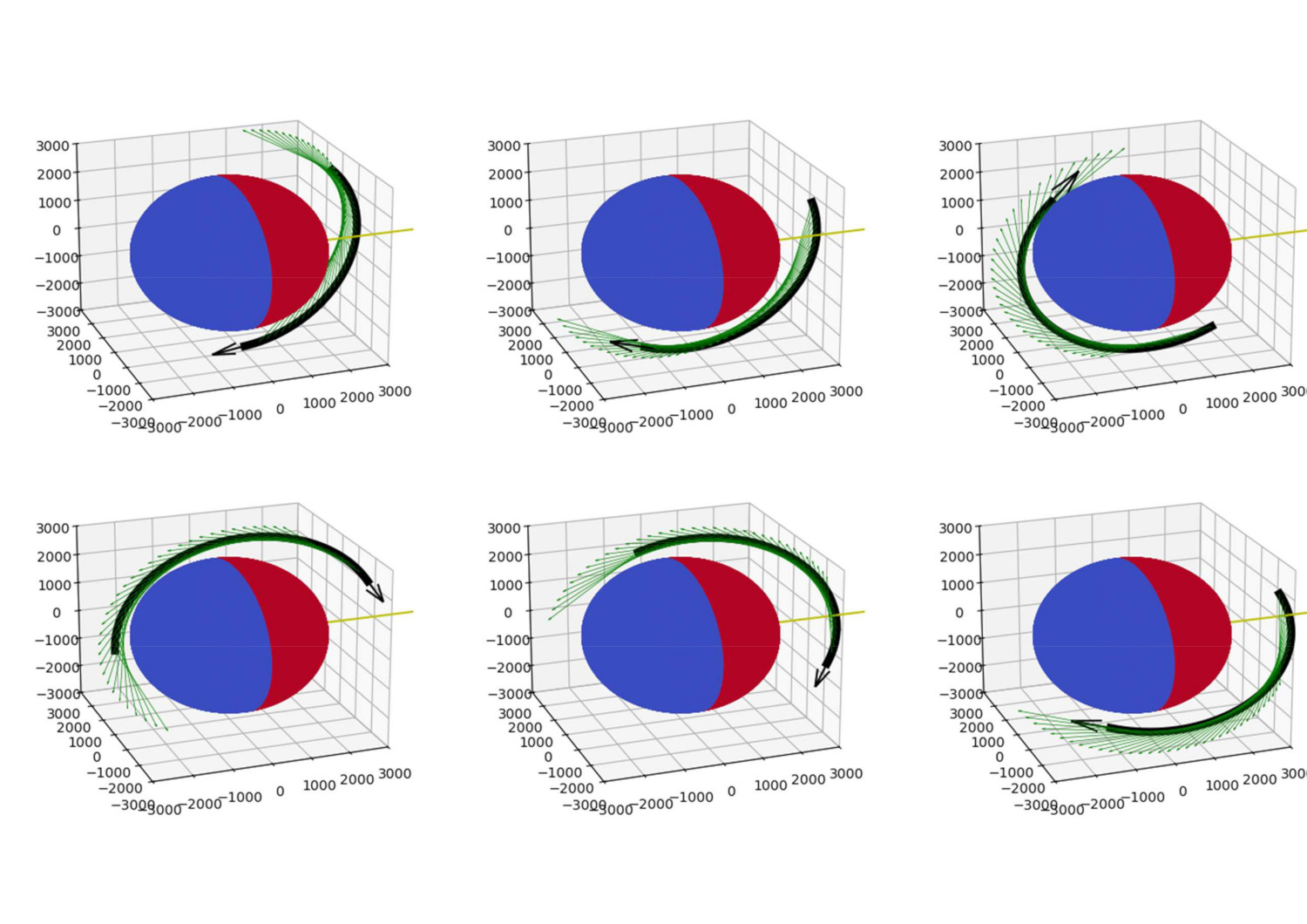
During MTP1 and MTP2, regular observations of the exosphere will be done from TAA ~ 170 – 30° to study the seasonal variations of the exosphere. Because of the numerous instrumental (illumination) and mission (e.g. telemetry) constraints, PHEBUS cannot operate all the time, and a careful study of the possibility of observations must be considered. We plan to perform one observation per orbit, i.e. ~ 10 observations per day (the orbital period of MPO is ~2.2 hours), including 8 observations dedicated to the exosphere and two other observations dedicated to star or interplanetary background. Only one channel (EUV or FUV) can be used during one observation with the two NUV channels. During one day, one observation is done with the EUV channel and seven observations with the FUV channel. However, the duration of one EUV observation is ~1 hour, while it is ~40 minutes with the FUV. The different observations are distributed along the orbit (Fig. 2) to have the best spatial coverage during one week. Examples of EUV observations during the short-term planning 8 (STP8) are shown on Fig. 2

Fig. 2 Example of 6 exospheric observations with the EUV channel during MTP2/STP8 (near Mercury’s perihelion. TAA between 340 and 23°). These observations cover the dayside (e.g. top left and middle panels), and partly the tail direction (top right, bottom left and right panels). The red color represents the dayside of Mercury, the blue surface the nightside. The sun direction is represented by the yellow arrow. The spacecraft orbit is represented by the black arrow and a few PHEBUS lines of sight during the observations are represented by the green arrows.

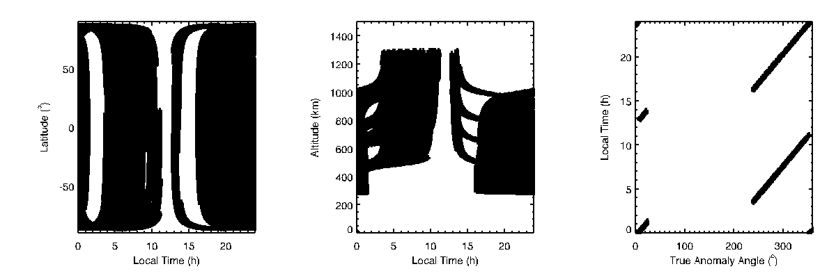
For each line of sight, we can define the altitude, local time and latitude of the tangent point. The expected coverage in local time and latitude during the medium-term planning 2 (MTP2: TAA 240°- 30°), assuming the current planification, is displayed on Fig. 3. This coverage can still be slightly modified due to changes in the planification. The predicted brightness of the different emissions, based on numerical model [7] will be also discussed during the presentation.

Fig. 3 Spatial and temporal coverage of the exospheric observations with the FUV detector during the MTP2. On the right panel, observations near the poles (latitude > 60°) are not considered.

Comparison with MESSENGER.

MESSENGER had a 12 hours periodic and highly elliptical orbit with its apoapsis (~15000 km) in the southern hemisphere and its periapsis (~200 km) near the north pole. Most of UVVS observations of the exosphere of Mercury occurred near apoapsis to have the largest coverage of altitudes (from ~ 200 to 2500 km) and local times but with a limited latitude coverage [8]. Due to the smaller orbit, PHEBUS/MPO altitude range will be reduced and limited to altitudes below ~ 1500 km. But PHEBUS will explore a larger range of latitude during one single observation at a fixed local time (Fig. 3 left). The local time coverage will be strongly dependent on the TAA, with observations near noon/midnight near Mercury’s perihelion and aphelion, and observations near terminator at TAA = 90 and 270° (Fig. 3 right). Therefore, the observations by PHEBUS will explore regions poorly sampled by MESSENGER/MASCS, offering the opportunity to distinguish between sputtering at high latitudes and dust impact or thermal desorption at mid and low latitudes.

References

[1] Chassefière, E. et al, Planet. Space Sci., 58, 201-223, (2010)

[2] Quémerais, E. et al., Space Sci. Rev., 216: 67, (2020)

[3] Quémerais, E., et al., J. Geophys. Res.: Planet, 128, e2023JE007743, (2023)

[4] Robidel, R., et al., , J. Geophys. Res. : Planets, 128, e2023JE007808, (2023)

[5] Suzuki, Y., et al., J. Geophys. Res.: Planets, e2024JE008524, (2024)

[6] Chaufray, J-Y., et al., J. Geophys. Res.: Planets, 128, e2022JE007669, (2023)

[7] Chaufray, J-Y, et al., Icarus, 384, 115081, (2022)

[8] McClintock, W.E., et al., Cambridge Planetary Science, Cambridge University Press, Cambride, 371-406., (2018)

How to cite: Chaufray, J.-Y., Quémerais, E., Koutroumpa, D., Robidel, R., Vontrat, A., Leblanc, F., Merusi, M., Laouisset, A., Yoshikawa, I., Yoshioka, K., Murakami, G., Suzuki, Y., Korablev, O., Belyaev, D., Ivanova, A., Pelizzo, M. G., and Corso, A.: Planification of the exospheric observations of Mercury by PHEBUS/BepiColombo during the first two months, Europlanet Science Congress 2026, The Hague, The Netherlands, 7–11 Sep 2026, EPSC2026-408, https://doi.org/10.5194/epsc2026-408, 2026.

EPSC2026-408

Download Close

Introduction

Next year, in 2027, the BepiColombo joint mission between the European Space Agency (ESA) and the Japan Aerospace Exploration Agency (JAXA) dedicated to the comprehensive exploration of the planet Mercury is set to enter its nominal phase. The SIMBIO-SYS instrument suite will act as the mission’s ‘eyes’, designed to provide comprehensive imaging and spectroscopic observations of the planet's surface through three independent optical channels.

The STereo imaging Channel (STC) is a core component for the SIMBIO-SYS suite objectives, designed specifically to achieve stereo global 3D mapping of Mercury and targeted color observations.  STC utilizes an innovative push-frame concept using a single detector but two separate optical paths, one tilted forward and one backwards, allowing stereo pairs to be captured by utilizing the movement of the satellite.  The instrument will generate a massive amount of data, in the order of hundreds of thousands of frames to complete the global mapping. This means that processing such large volumes of data for mosaicking and stereogrammetry will require a pipeline that is as robust and automated as possible, currently being developed by the INAF OAPd team.

Processing Pipeline Overview

Due to the orbital geometry and planning conditions, the frame footprints of the two channels will not align perfectly, so the mosaicking and stereometric processing will be carried out in blocks. This also has the advantage of simultaneously improving attitude and position information through bundle block adjustment, thereby mitigating artefacts caused by inaccuracies in kernels and surface models. In the pipeline, the Mercury’s surface will be dynamically tessellated into rectangles of approximately 5 x 5 frames, varying according to the geometric conditions, for each channel and with an appropriate lateral overlap to avoid geometric inconsistencies (such as gaps) and facilitate subsequent mosaicking. The pipeline will ingest the images after being radiometrically corrected, as well as the initial orbital pointing data expressed in the Mercury body-fixed Cartesian frame. Intrinsic camera parameters (focal length, principal point, distortion) are obtained from validated pre-flight calibration data.

The frames block is geometrically refined through a progressive “middle-out” bundle adjustment strategy. Starting from the central image and expanding outward bilaterally (both horizontally and vertically), successive adjacent frame pairs are matched using SIFT-based feature detection [3]. Corresponding image points are back-projected onto a reference Mercury global DTM (at 663 m/px) [4]  to establish absolute 3D tie-point coordinates, anchoring the adjustment to the hermean topography. A Ceres-based nonlinear least-squares solver [5] minimizes reprojection residuals jointly over the expanding set of image poses, while previously corrected frames are held fixed to prevent sequential drift. The resulting projection matrices define the rectified mosaics geometry.

Following the mosaicking process, a second alignment stage allows any residual errors between the two mosaics to be corrected. In this stage, the mosaic from the second channel is aligned with the first using a similar pre-alignment and bundle adjustment procedure as for the single frames.  

For an initial, coarse matching, a tile-based SIFT is used, whereby the mosaics are divided into subsets that are compared in parallel. This allows tie points to be defined as uniformly and evenly as possible across the images being processed. The stereo processing part is a direct evolution of the 3DPD software, which has been under active development since 2018 [1][2], for processing DTMs from the CaSSIS (Colour and Stereo Surface Imaging System) instrument aboard ESA’s Trace Gas Orbiter. The CaSSIS instrument, in fact, acquires stereo imagery using a similar push frame architecture, in which the two acquision of the stereo pair are read out during a single spacecraft overpass, yielding a forward/backward stereo pair using a rotation mechanism. 

In the 3DPD, the seed points information obtained with SIFT is expanded to the whole image using Delaunay triangulation, resulting in a TIN surface of parallaxes, represents the first sparse disparity maps used as initialization for the subsequent dense matching process. The dense matching phase employs multi-scale processing, utilizing image pyramids to implement a coarse-to-fine strategy. This approach effectively constrains search space and minimizes matching outliers (blunders) under the hypothesis that the target is continuous. The process begins at the coarsest pyramid level using Normalized Cross-Correlation (NCC) for initial matching. These results are then propagated to successively higher resolutions: at each stage, the disparities for new points are estimated through bilinear interpolation of their neighbors. This iterative refinement continues until the highest resolution level is reached, where Least-Squares Matching (LSM) is applied to achieve final sub-pixel precision [6].

Using the previously corrected projection matrices, the point cloud derived from dense matching can finally be projected into a chosen reference system, thereby refined in the post-processing and interpolated into a DTM and orthorectified image blocks.

Testing

Active development of the pipeline is facilitated by two different test datasets, which enable its effectiveness to be assessed and fine-tuning to be carried out before the arrival of STC data: synthetic images generated using the PLanetary Image Simulator (PLAS) [7]  and the images of Mars from the CaSSIS instrument. PLAS enables the creation of synthetic images that faithfully reproduce the format and characteristics of STC data. The images are generated by faithfully reproducing the lighting and attitude conditions derived from the SPICE kernels, using as the surface three-dimensional surface models of the Moon and Mercury. Furthermore, the simulated images allow for the controlled testing of pointing errors and noise, to quantify their impact. Regarding CaSSIS, although the target (Mars) and ground resolution differ by approximately an order of magnitude (approximately 4.5 m/px CaSSIS), the use of real data allows for the handling of unforeseen errors in the kernels and the presence of unexpected noise.

[1] Simioni, E., Re, C., Mudric, T., et al. (2021). PSS 198, 105165. https://doi.org/10.1016/j.pss.2021.105165

[2] Re, C., Fennema, A., Simioni, E., et al. (2022). PSS 219, 105515. https://doi.org/10.1016/j.pss.2022.105515

[3]  Lowe, D.G. (2004). IJCV 60, 91–110. https://doi.org/10.1023/B:VISI.0000029664.99615.94

[4]  Becker, K. J., Robinson, M. S., Becker, T. L et al. (2016). 47^th LPSC

[5] Agarwal, S., Mierle, K., & The Ceres Solver Team. (2023). Ceres Solver (Version 2.2). https://github.com/ceres-solver/ceres-solver

[6] Gruen (1985) S. Afr. J. Photogramm. Remote Sens. Cartogr. 14.3 175-187.

[7] Re, C., Tullo, A., La Grassa, R., et al. (2024). EPSC2024-851. https://doi.org/10.5194/epsc2024-851

How to cite: Tullo, A., Re, C., Simioni, E., and Cremonese, G.: Toward a Robust Pipeline for the 3D Reconstruction Of The Hermean Surface: The SIMBIO-SYS STC Automated Processing Framework, Europlanet Science Congress 2026, The Hague, The Netherlands, 7–11 Sep 2026, EPSC2026-585, https://doi.org/10.5194/epsc2026-585, 2026.

EPSC2026-585

Download Close

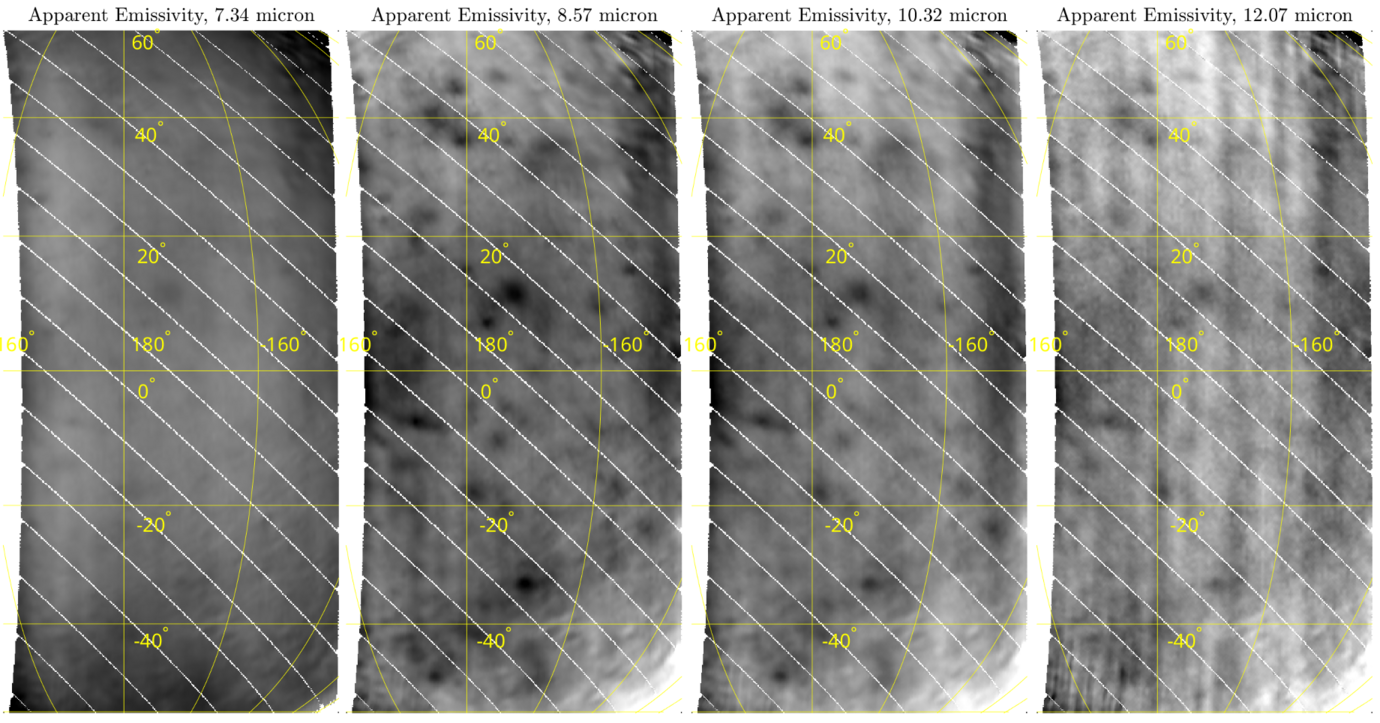
The Mercury Radiometer and Thermal Infrared Spectrometer (MERTIS) is part of the payload on the joint ESA/JAXA mission BepiColombo to Mercury. The onboard spectrometer will map the thermal emissivity of Mercury in the 7-14 µm wavelength range [1]. Understanding how Mercury's surface properties influence remote sensing data is essential for interpreting the data of MERTIS. Therefore, to support the interpretation of MERTIS data, various emissivity measurements already have been performed at the Planetary Spectroscopy Laboratory (PSL) at the German Aerospace Center (DLR) in Berlin [2]. This study aims to extend the knowledge acquired by systematically investigating the effect of grain size on emissivity and bidirectional reflectance spectra of Mercury analogue mixtures. 

Two endmembers, an enstatite and an anorthoclase, were prepared in three grain size fractions: 0–25 µm, 25–63 µm, and 125–250 µm. In addition to the pure endmembers, intimate mixtures of the two endmembers with ratios of 25:75, 50:50, and 75:25 were created, including both homogeneous and heterogeneous grain size combinations, resulting in a total of 33 samples.

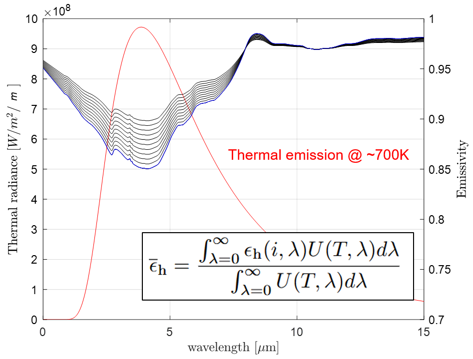
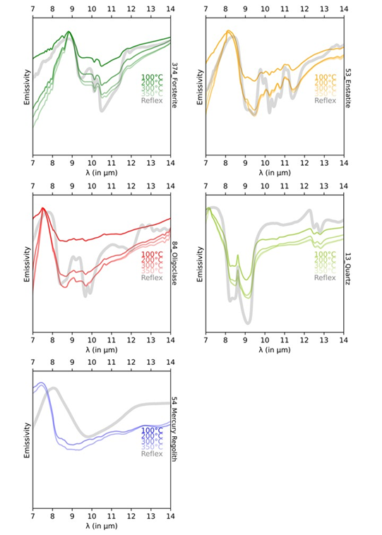
Mid-infrared emissivity spectra were acquired at 150 °C, 250 °C, 350 °C, and 450 °C under simulated Mercury pressure condition (0.7 mbar) in the DLR-built emissivity chamber at PSL. The sample spectra were calibrated using emissivity spectra of a graphite slab serving as approximation of a blackbody, and additional hemispherical reflectance spectra of the samples, which were taken under ambient temperature conditions (Fig. 1).

Figure 1: Sample measurements (thick lines) with approximated blackbody target measurements (color gradient) for data calibration.

In addition to the emissivity measurements, bidirectional reflectance spectra of the same samples were acquired across a wide spectral range (VIS to MIR). Spectra were taken before and after heating in the emissivity chamber to investigate the influence of heating upon the samples. Next to the chamber-heated samples, fresh sample of all mixtures were measured in a vacuum-oven under the same temperature and lower pressure condition as in the emissivity chamber. The oven-heated samples were used to additionally investigate the influence of sample preparation and sample handling on the spectra. Those samples are in fact directly heated in the vacuum oven inside their sample holders, while in the case of the sample measured in bidirectional reflectance after the emissivity measurements, those powders are scooped into the reflectance sample holder from the emissivity sample cup, this process altering the original layering inside the sample because of the thermal gradient inside the powdered samples heated in vacuum. All bidirectional reflectance spectra were merged, creating one full wavelength-range spectrum for each sample (Fig. 2).

Figure 2: Bidirectional reflectance spectra from UV to MIR before (left) and after (right) calibration.

The results show that grain size systematically influences spectral features, particularly the peak width of the Christiansen Feature and the occurrence of Transparency Feature in the emissivity measurements, as well as their maximum emissivity value. Spectral behavior is influenced by clinging fines, scattering regimes, and thermal gradients. In addition, both the emissivity and reflectance data show that spectral properties and trends are strongly related to relative grain size, and especially in the mixtures, the appearance of features is linked to the endmember with the smaller grain size (Fig. 3). Furthermore, oven-heated samples show more consistent results than chamber-heated samples, highlighting the importance of sample preparation and handling.

This study demonstrates systematic grain size effects and identifies robust grain size indicators in intimate mixtures. The findings of this study highlight the need to consider these grain size effects when interpreting remote sensing spectra of Mercury to contribute to a more reliable interpretation of spectral data from MERTIS and other spectral suites onboard the BepiColombo mission. Additionally, the results highlight the need for consistent sample handling in laboratory set-ups.

References:

[1]       H. Hiesinger and J. Helbert, “The Mercury Radiometer and Thermal Infrared Spectrometer (MERTIS) for the BepiColombo mission,” Planet. Space Sci., vol. 58, no. 1–2, pp. 144–165, Jan. 2010, doi: 10.1016/j.pss.2008.09.019.

[2]       A. Maturilli, J. Helbert, I. Varatharajan, and H. Hiesinger, “Emissivity Spectra of Analogue Materials at Mercury P-T Conditions,” presented at the 48th Annual Lunar and Planetary Science Conference, Mar. 2017, p. 1427. Accessed: Sep. 24, 2025. 

How to cite: Lamers, G., Maturilli, A., Alemanno, G., Van den Neucker, A., Adeli, S., and Harald, H.: Influence of Particle Size in Laboratory Emissivity of Mercury Analogue Material Mixtures under Simulated Mercury Conditions, Europlanet Science Congress 2026, The Hague, The Netherlands, 7–11 Sep 2026, EPSC2026-162, https://doi.org/10.5194/epsc2026-162, 2026.

EPSC2026-162

Download Close

Mercury's surface is classified into several units according to its geological (Denevi et al., 2013), compositional (Weider et al., 2015, Vander Kaaden et al., 2017, Peplowski et al., 2019), and spectral properties (Robinson et al., 2008, Denevi et al., 2009, Murchie et al., 2015). Units do not necessarily correlate, limiting our understanding of the geological history of the planet. Several processes act simultaneously to modify the spectral properties of Mercury, which complicates the identification of the origin of the spectral units. Isolating the contribution of each process requires laboratory experiments that aim to reproduce Mercury-like conditions as closely as possible. As an airless body, Mercury is subject to space weathering leading to modifications in the surface spectral properties. Laboratory spectral studies of space weathering effects on Mercury analogues are typically conducted under a single geometrical configuration (Caminiti et al., 2024), which limits direct comparison with remote sensing observations (Rubino et al., 2022). Remote sensing instruments onboard space missions frequently observe the same area at different local times and from varying angles (incidence, emission, and phase angles), resulting in measurements acquired under diverse geometrical conditions. Constraining the effects of the geometry of observation of the space-weathered surface of Mercury is particularly relevant in the context of the ESA-JAXA-BepiColombo mission (Benkhoff et al., 2021), which will reach Mercury's orbit in 2026. The Visible Infrared Hyperspectral Imager (VIHI) channel (Filacchione et al., 2023) from the Spectrometers and Imagers for MPO BepiColombo Integrated Observatory SYStem (SIMBIO-SYS) payload (Cremonese et al., 2020) will map the surface from the visible to near-infrared (400-2000 nm). SIMBIO-SYS will operate in nadir-pointing configuration with variations of the incidence angle and the possibility of off-pointing to measure specific targets of interest during the extended phase of the mission. These observational conditions differ significantly from the NASA-MESSENGER-MASCS instrument's measurements obtained at large phase angles (Izenberg et al., 2014). To compare both datasets and eventually observe changes at the surface of Mercury in the last decade, additional laboratory activities are required. This study presents the VISNIR spectral analysis of a Mercury simulant to understand the impact of space weathering and observation geometries on the spectral properties of Mercury surface.

We used the “Mercury mix” simulant combining aubrite material with natural and synthetic minerals to better reproduce the composition of Mercury's crust (Leon-Dasi et al., 2025). We performed ion irradiation using the SIDONIE electromagnetic isotope separator (IJCLab, France) (Chauvin et al., 2004) interfaced with the INGMAR (IrradiatioN de Glaces et Météorites Analysées par Réflectance VIS-IR, IAS, France) vacuum chamber (P ~10^-7 mBar) (Lantz et al., 2017). We used 20 keV He⁺ with fluence up to 10¹⁷ ions/cm². Bidirectional reflectance spectroscopy was performed at IPAG (France) using the SHADOWS spectro-gonio radiometer (Potin et al., 2018) to analyze the effect of the geometrical configuration. The illumination angle ranged from the nadir to grazing illumination (0°, 20°, 40°, and 60°). For each illumination angle, we acquired spectra with an observation angle of ~ -70° to +70°. Spectra were acquired at room temperature, in the visible to near-infrared (600-2000 nm).

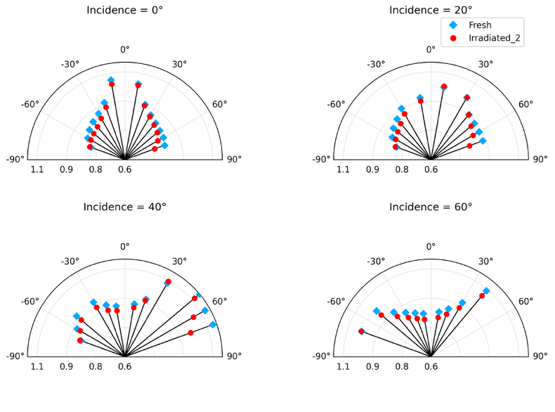
The BRDF shows an increase in reflectivity around the specular configuration (e~ i) with an angular width of about 20°, and towards e~-i for large incident angles (Figure 1). R750 and R1450 both decrease with increasing phase angle until ~70° (backscattering) and increases towards higher phase angles (forward scattering). The analog presents a darkening in the VIS (R750) which is limited in specular conditions (Figure 1), a reddening in the VISNIR (VISNIR_Slope) after 20° from specular conditions, and a possible brightening in the NIR (R1450) after ion irradiation. The effects of ion irradiation on the reflectance are stronger with increasing phase angle (Figure 1). Thus, we expect future SIMBIO-SYS data to be less sensitive to space weathering than MASCS data. The fresh sample shows few changes in spectral slope induced by the observation geometry. This supports the idea that slope changes are poorly affected by the emission angle compared to changes in reflectance (Leon-Dasi et al., 2025). However, the irradiated sample is more sensitive to variations in emission angle.

Overall, the measurements demonstrate that irradiation‑induced changes in spectral parameters are strongly dependent on observation geometry. Under certain geometries, fresh and weathered units can appear spectrally similar, while under others they diverge markedly. These results identify optimal viewing conditions to assess space‑weathering effects on Mercury’s surface, providing timely constraints on surface evolution and valuable guidance for BepiColombo science off‑pointings.

Figure 1: Evolution of the normalized reflectance at 750 nm under different optical geometries for fresh and He⁺-implanted pellets. Uncertainties are not visible; this indicates that they are smaller than the symbol.

References:
- Benkhoff et al., Space Sci. Rev. 217.8, 90 (2021).
- Caminiti et al., Icarus 420, 116191 (2024).
- Chauvin et al., Nucl. Instrum. Methods Phys. Res. A 521.1, 149–155 (2004).
- Cremonese et al., Space Sci. Rev. 216.5, 75 (2020).
- Denevi et al., JGR Planets 118.5, 891–907 (2013).
- Denevi et al., Science 324.5927, 613–618 (2009).
- Filacchione et al., IEEE Trans. Geosci. Remote Sens. 61, 1–12 (2023).
- Izenberg et al., Icarus 228, 364–374 (2014).
- Lantz et al., Icarus 285, 43–57 (2017).
- Leon-Dasi et al., Icarus 436, 116582 (2025).
- Murchie et al., Icarus 254, 287–305 (2015).
- Peplowski & Stockstill-Cahill, JGR Planets 124.9, 2414–2429 (2019).
- Potin et al., Appl. Opt. 57.28, 8279–8296 (2018).
- Robinson et al., Science 321.5885, 66–69 (2008).
- Rubino et al., Icarus 376, 114887 (2022).
- Vander Kaaden et al., Icarus 285, 155–168 (2017).
- Weider et al., Earth Planet. Sci. Lett. 416, 109–120 (2015).

How to cite: Caminiti, E., Leon-Dasi, M., Lantz, C., Brunetto, R., Beck, P., Besse, S., Cartier, C., Llado, L., Doressoundiram, A., and Benkhoff, J.: Effects of observation geometry on the visible to near-infrared spectra of a space-weathered Mercury simulant, Europlanet Science Congress 2026, The Hague, The Netherlands, 7–11 Sep 2026, EPSC2026-176, https://doi.org/10.5194/epsc2026-176, 2026.

EPSC2026-176

Download Close

How to cite: Verkercke, S., Hadid, L., Aizawa, S., Delcourt, D., Raines, J., Fränz, M., Saito, Y., Yokota, S., Rojo, M., Harada, Y., Fontaine, D., André, N., Katra, B., Verdeil, C., Modolo, R., Krupp, N., Leblanc, F., Fiethe, B., and Fischer, H.: Statistical Noise Removal Method for the Mass Spectrum Analyzer onboard BepiColombo/Mio, Europlanet Science Congress 2026, The Hague, The Netherlands, 7–11 Sep 2026, EPSC2026-327, https://doi.org/10.5194/epsc2026-327, 2026.

EPSC2026-327

Download Close

Mercury is the most chemically distinctive terrestrial planet in the Solar System. Its large metallic core, thin silicate shell, low-FeO surface composition, high sulfur content, and volatile-rich geochemistry are often discussed as separate anomalies (Cartier and Wood, 2019). Here, we test whether these properties are instead linked expressions of a single formation pathway: accretion and differentiation under highly reducing conditions. In this framework, Mercury is not an Earth-like planet with an unusually large core, but rather an end-member reduced planet and the Solar System benchmark for a broader class of rocky worlds, including possible exo-Mercuries.

Because no confirmed Mercury meteorites are available, several reduced precursor materials have been proposed as Mercury analogues, including aubrites and ultramafic reduced achondrites such as diopsidites (e.g., Malavergne et al., 2010; Cartier and Wood, 2019; Anzures et al., 2020; Steenstra and van Westrenen, 2020). In this work, these differentiated reduced meteorites are used as analogues for plausible inner-disk building blocks. Their pyroxene-dominated mineralogy, minor sulfides, and lack of plagioclase provide a natural starting point for testing reduced mantle compositions. Nucleosynthetic systematics further link these reduced planetesimals to an inner-disk reservoir relevant to Mercury, while Mg isotope constraints indicate that ²⁶Al alone was insufficient to drive widespread melting. Instead, extensive differentiation likely required protracted growth, impact heating, and gravitational energy release during the assembly of Moon- to Mercury-scale bodies.

After constraining the mineralogical and isotopic properties of these reduced precursor materials, and having shown through nucleosynthetic fingerprinting that they sample an inner-disk non-carbonaceous reservoir relevant to Mercury, we then used their bulk compositions as inputs for thermodynamic phase-equilibrium modelling. This step anchors the inferred interior mineralogy of Mercury to building blocks that plausibly formed in the innermost regions of the solar nebula, the likely accretion environment of the planet.

Thermodynamic phase-equilibrium modelling with Perple_X (Connolly, 1990) shows that reduced Mercury-like bulk compositions do not produce Earth-like peridotitic mantles. Across the investigated CH-like, aubrite-like, and reduced enstatite-like compositions, orthopyroxene plus clinopyroxene exceed olivine, yielding FeO-poor, sulfur-bearing, pyroxene-rich mantle assemblages, consistent with recent experimental findings (Boujibar et al., 2025). This result is central because it affects the planet’s density structure, solidus, melt productivity, viscosity, and thermal evolution (Cioria et al., 2024). Applying terrestrial olivine-controlled rheology to Mercury therefore introduces first-order inconsistencies: Mercury’s mantle is likely governed by a different compositional and rheological regime. The same framework predicts that melts extracted from reduced, pyroxene-rich mantles crystallize into crustal cumulates ranging from noritic to gabbroic compositions. These crustal products are FeO-poor, Mg-rich, and dominated by pyroxene and plagioclase, rather than resembling typical terrestrial basaltic crust.

Overall, this work supports a nebula-driven, selectively accreted reduced lineage for Mercury, in which the planet’s present-day structure reflects not only post-accretion differentiation, but also the geochemical nature of the materials from which it formed. In this framework, Mercury’s large core, FeO-poor silicate shell, sulfur-bearing mineralogy, and pyroxene-rich mantle are interpreted as inherited consequences of accretion from highly reduced inner-disk building blocks, rather than as features that must be produced exclusively by catastrophic mantle stripping (e.g., Benz et al., 1988). The predicted low-FeO, pyroxene-rich lithologies, systematic Mg/Si and Ca/Si domains, silica-rich components, and density contrasts provide testable targets for BepiColombo. More broadly, if comparable reducing environments existed in the inner regions of other planetary systems, the same meteorite-constrained thermodynamic workflow can be extended to rocky exoplanets that formed from similarly reduced reservoirs. In this sense, Mercury is not only an anomaly of the Solar System, but a local expression of a broader planetary outcome: rocky planet differentiation controlled by formation region, precursor chemistry, and redox state.

Acknowledgments: G.M. and C.C. acknowledge support from the Italian Space Agency (2022-16-HH.1-2024).

References:

Anzures, B. A., Parman, S. W., Milliken, R. E., Namur, O., Cartier, C., & Wang, S. (2020). Effect of sulfur speciation on chemical and physical properties of very reduced mercurian melts. Geochimica et Cosmochimica Acta, 286, 1–18. https://doi.org/10.1016/j.gca.2020.07.024

Benz, W., Slattery, W. L., & Cameron, A. G. W. (1988). Collisional stripping of Mercury's mantle. Icarus, 74(3), 516–528. doi: 10.1016/0019-1035(88)90118-2

Boujibar, A., Righter, K., Fontaine, E., Collinet, M., Lambart, S., Nittler, L. R., & Pando, K. M. (2025). A Pyroxenite mantle on Mercury? Experimental insights from enstatite chondrite melting at pressures up to 5 GPa. Icarus, 437, 116602. doi: 10.1016/j.icarus.2025.116602

Cartier, C., & Wood, B. J. (2019). The role of reducing conditions in building Mercury. Elements,15(1), 39-45.doi: 10.2138/gselements.15.1.39

Cioria, C., Mitri, G., Connolly, J. A. D., Perrillat, J.-P., & Saracino, F. (2024). Mantle mineralogy of reduced sub-Earths exoplanets and exo-Mercuries. Journal of Geophysical Research: Planets, 129(7), e2023JE008234. doi: 10.1029/2023JE008234

Connolly, J. A. D. (1990). Multivariable phase diagrams; an algorithm based on generalized thermodynamics. American Journal of Science, 290(6), 666–718. https://doi.org/10.2475/ajs.290.6.666

Malavergne, V., Toplis, M. J., Berthet, S., & Jones, J. (2010). Highly reducing conditions during core formation on Mercury: Implications for internal structure and the origin of a magnetic field. Icarus, 206(1), 199–209. https://doi.org/10.1016/j.icarus.2009.09.001

Steenstra, E. S., & Van Westrenen, W. (2020). Geochemical constraints on core-mantle differentiation in Mercury and the aubrite parent body. Icarus, 340, 113621. doi: 10.1016/j.icarus.2020.113621

How to cite: Cioria, C. and Mitri, G.: Mercury and exo-Mercury interiors constrained by reduced meteorite analyses and thermodynamic modelling, Europlanet Science Congress 2026, The Hague, The Netherlands, 7–11 Sep 2026, EPSC2026-376, https://doi.org/10.5194/epsc2026-376, 2026.

EPSC2026-376

Download Close

The forthcoming orbital phase of the ESA/JAXA mission BepiColombo is expected to provide new and updated constraints on Mercury’s interior structure and evolution, highlighting the need to reassess and strengthen existing thermal evolution models. Significant uncertainties remain regarding the thermal, transport and elastic properties of Mercury’s mantle and core. Notably, the mantle composition is poorly known. It could be composed of variable proportions of forsterite and enstatite [1], which exhibit markedly different thermal conductivities and rheological behavior [2, 3]. The core can be approximated as an Fe-Si alloy, although it likely also contains other light elements such as S and C. Yet, the core Si fraction is also uncertain and substantially impacts key properties such as density, liquidus, entropy, and thermal conductivity [4]. To restrict the range of uncertainties regarding these parameters, we conducted an extensive set of Monte-Carlo simulations of the coupled core-mantle thermal evolution of Mercury, filtering the results according to various combinations of observational constraints whose choice can significantly influence the number of successful models and their typical evolution.

We employed a 1D parameterized mantle convection model (TEMPURA [5]) in which we incorporated the influence of pressure- and temperature-dependent thermal conductivity, heat capacity, thermal expansivity, and density for forsterite, enstatite, and diopside, which we considered in variable proportions. We coupled this mantle model with an evolution model of the core simulating inner core crystallization and the development of a thermally stratified layer at the top of the liquid core [6] using  self-consistent Fe-Si thermodynamic properties.

We conducted Monte-Carlo simulations of Mercury’s thermal evolution, varying the following mantle parameters: initial temperature profile, forsterite over enstatite ratio, reference mantle viscosity, and crustal enrichment factor in heat-producing elements. Additionally, we varied some core parameters: starting core-mantle boundary (CMB) temperature, core radius, thermal conductivity, and melting entropy.

We filtered the models based on the following observational constraints: (1) final crust thickness between 15 and 60 km; (2) onset of global contraction within the first 500 Myr; (3) dynamo generation between 500 and 1000 Myr and at the present day; (4) bulk of the volcanic crust produced within the first   Gyr, and (5) contraction accumulating at a decreasing rate over the evolution.

Models that satisfy constraints (1), (2), and (3) exhibit a high reference viscosity (10²² Pa s), low initial CMB temperature (< 2000 K), a  core radius between 2000 and 2010 km, and require a high core melting entropy, and a low core thermal conductivity. The initial mantle temperature, mantle enstatite fraction, and crustal enrichment factor are less decisive. Upon including  the constraint (4) and (5), the results shift to lower reference viscosities (10²¹ Pa s) and large crustal enrichment factors (>7).

These discrepancies can be understood in terms of the competing thermal effects imposed by the different constraints. High reference viscosities inhibit efficient planetary cooling, which facilitates the maintenance of a convective layer in the core for 4.5 Gyr, a prerequisite for the current dynamo (3). However, higher reference viscosities (10²³ Pa s) also suppress melt production, leading to crustal thicknesses that are too small to satisfy the constraint (1), and may even produce early-stage expansion, inconsistent with constraint (2). Low initial CMB temperatures are essential for nucleating the inner core before 1 Gyr, which is an important driver for the ancient dynamo (3). Imposing the additional requirement that the bulk of the crust and contraction forms within the first Gyr (4-5) shifts the preferred solutions to  lower reference viscosities and higher enrichment factors, both of  which promote efficient mantle cooling.

In summary, the different observational constraints favor markedly different mantle and core properties, highlighting the challenge of  reproducing Mercury’s volcanic, tectonic, and magnetic evolution within a single thermal history model. 

Therefore, accurately characterizing Mercury’s interior evolution requires a careful assessment of which observations are most robust and how they should be incorporated into thermal evolution models.

[1] Saracino et al. (2025). Chem. Geol., 683, 122777, doi: 10.1016/j.chemgeo.2025.122777. [2] Zhang et al. (2019). Earth Planet. Sci. Lett., 519, 109-119, doi:10.1016/j.epsl.2019.04.048. [3] Guo et al. (2024). Geochem. Geophys. Geosyst., 25(6), e2023GC011419, doi:10.1029/2023GC011419. [4] Edmund et al. (2022). Nature Comm., 13, 387, doi:10.1038/s41467-022-27991-9. [5] Baumeister et al. (2023). A\&A, 675, A122, doi:10.1051/0004-6361/20224579. [6] Davies et al. (2024). Earth Planet. Sci. Lett., 641, 118812, doi:10.1016/j.epsl.2024.118812.

How to cite: Lécaille, M., Tosi, N., Rivoldini, A., Baumeister, P., Namur, O., and Charlier, B.: Disentangling the influence of observational constraints on Mercury's interior evolution, Europlanet Science Congress 2026, The Hague, The Netherlands, 7–11 Sep 2026, EPSC2026-648, https://doi.org/10.5194/epsc2026-648, 2026.

EPSC2026-648

Download Close

Due to MESSENGER’s elliptical orbit, Mercury's gravity field is unevenly known with resolution ranging from up to only about spherical harmonic degree 10 (∼1,500 km wavelength) in the southern hemisphere to degree 90 and up to 160 in the north (∼100–170 km; [1]). Such low-resolution gravity field represents a major obstacle to our understanding of the planet's interior structure and geodynamic history [2]. One objective of the BepiColombo mission is to improve Mercury's gravity field models using the Mercury Orbiter Radio Science Experiment (MORE) [3]. However, even after the extended mission, the gravity field is predicted to only reach about degree 40-50 globally. Some previous works have attempted to increase the resolution of the gravity field based on the expectation that, at sufficiently high harmonic degree, gravity should be correlated to topography [4]. Yet, at the measured wavelengths on Mercury, lithosphere deformations from geologic loads are expected to prominently affect the planet's gravity field, making gravity-from-topography models highly non-unique [2,4]. 

Before high-resolution gravity measurements were made available on the terrestrial planets, studies have commonly used elevation data and tectonic structures to investigate lithosphere deformations and the presence of subsurface loads [5]. Detailed characterization of subsurface loads and lithosphere deformations can in turn be used to break part of the non-uniqueness in the predicted, high-degree gravity, field.  In this work, we combine topography data and tectonic deformations [6,7] together with a lithosphere loading model [8] to provide high-resolution gravity field and interior structure models of Mercury.

Using a global tectonic catalog together with analysis of elevation profiles across tectonic landforms, our previous works have estimated lateral variations in tectonic strain [6,7]. The estimated average shortening reflects Mercury’s global contraction (with values of ranging from 6 to 8 km), while lateral variations have been attributed to local lithosphere deformations from geologic loads [7]. While lateral cooling efficiency due to crustal thickness or surface temperature variations can induce lateral variations in planetary contraction, these effects are expected to only moderately affect contraction [9] and would not fully explain the observed large variations. Here, we convert the estimated tectonic strain to membrane–flexural uplift and subsidence using a spectral transfer function similar to an admittance [7]. Lithosphere displacements are then used together with topography data to predict high-resolution gravity field models of Mercury. The models are patched to MESSENGER's observed gravity field based on the local degree-strength. A by-product of this inversion is the planet’s interior structure, consisting here of a crust with laterally variable thickness and mantle with laterally variable density.

The estimated gravity field and interior structure maps will be presented at the conference.

[1] Genova et al. (2023), Icarus, 10.1016/j.icarus.2022.115332.

[2] Broquet et al. (2025), JGR: Planets, 10.1029/2025JE009139.

[3] Iess et al. (2021), SSR, 10.1007/s11214-021-00800-3.

[4] Goossens et al. (2017), JGR: Planets, 10.1002/2017GL074172.

[5] Solomon & Head (1980), Rev. Geophys. 10.1029/RG018i001p00107.

[6] Broquet & Andrews-Hanna (2026a), JGR: Planets, 10.1029/2025JE009584.

[7] Broquet & Andrews-Hanna (2026b), JGR: Planets, 10.1029/2025JE009585.

[8] Broquet (2024). 10.5281/zenodo.10552129

[9] Büttner et al. (2026). EPSC26.

How to cite: Broquet, A., Cascioli, G., Genova, A., Hussmann, H., Iess, L., Thomas, N., and Wieczorek, M.: Mercury's gravity field as constrained by the tectonic record, Europlanet Science Congress 2026, The Hague, The Netherlands, 7–11 Sep 2026, EPSC2026-372, https://doi.org/10.5194/epsc2026-372, 2026.

EPSC2026-372

Download Close

Mercury’s geodynamic history has been characterized by global contraction due to planetary cooling and inner core growth. The planet likely experienced the largest radius change out of all Solar System bodies, with most occurring early in its thermal evolution (Watters, 2021, Peterson et al., 2021, Grott et al., 2011, Byrne et al., 2014). Such contraction has been recorded in tectonic landforms on the surface, which can be used to reconstruct radius changes from tectonic strain. However, estimates substantially vary between < 2 km (Watters, 2021) and up to 7 km (Byrne et al., 2014), depending on whether wrinkle ridges are taken into account as contributing to global contraction. A recent study by Broquet & Andrews-Hanna (2026) revisited Mercury’s tectonic record and found global contraction values of 8.3 ± 4.5 km, with a conservative range of 6.3 ± 3.2 km when considering only primary tectonic landforms. Contraction was found to substantially vary spatially, with some regions displaying a near‐zero record of contraction. The authors also propose high contraction rates of 0.02 – 0.04 km/Myr from 4.1 – 3.9 Ga, followed by significantly lower contraction rates during the later evolution. Additionally, an upcoming study by Nishiyama et al. (submitted) suggests that surface roughness can obscure tectonic features on the surface, leading to an underestimation of Mercury’s global contraction by up to 30 %.

Motivated by these new findings, this study uses 3D geodynamic simulations to model Mercury’s thermal evolution and estimate contraction on a global and local scale. Our geodynamic models build upon the work of Fleury et al. (2024) and use the finite-volume mantle convection code GAIA (Hüttig et al., 2013). GAIA solves the conservation equations of mass, momentum and energy from 4.5 Ga to present day under the assumption of homogeneous mantle composition, Newtonian rheology, and negligible inertia. In our models, we employ surface temperature variations caused by the combined effects of Mercury’s low obliquity and its 3:2 spin-orbit resonance (Vasavada et al., 1999), as well as crustal thickness variations, inverted from gravity and topography data (Broquet et al., 2024).  We account for a laterally variable crustal thermal conductivity considering crustal porosity variations (Broquet et al., 2024). We use two transfer models by Henke et al. (2016) to replicate the decrease of thermal conductivity with increasing porosity, and also consider an insulating megaregolith layer of 2 – 5 km thickness. Additionally, we investigate the effects of mantle melt extraction on regional contraction. While previous models (Peterson et al., 2021; Tosi et al., 2025) have considered only fully extrusive scenarios, we test both intrusive and extrusive cases, varying global and local intrusive to extrusive ratios between 0 and 1. We place magmatic intrusions either at a predefined depth within the lithosphere (i.e., varying between 45 and 140 km) or, for some cases, we place them at the base of the crust, which naturally leads to spatial variations of the intrusive melt depth. We compare our predictions for present-day global and local contraction to tectonic strain from Broquet & Andrews-Hanna (2026). 

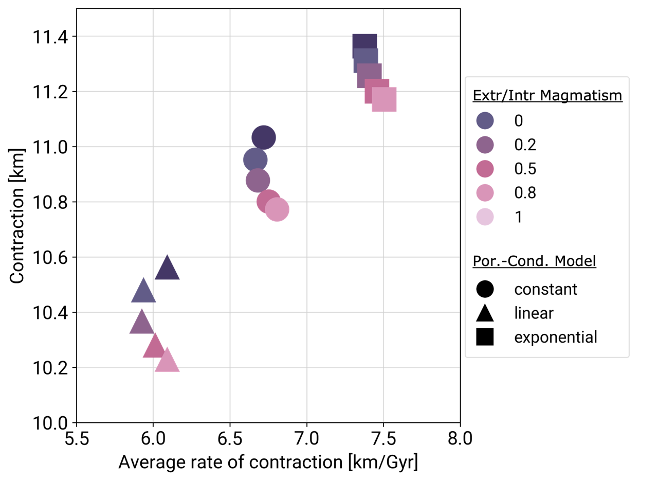
Our models predict between 7 – 12 km of global contraction between the end of crustal formation (3.8 Ga) and today, with an average of 9.8 ± 1.3 km. Although increasing the average crustal thickness strongly reduces the early contraction rate, it is found to have no significant impact on overall global contraction estimates. We find that regions insulated by a thick, porous crust, especially located around the two hot poles (60°S - 60°N), are warmer during early evolution, inducing higher and longer melt production. Melt extraction in these areas leads to more efficient cooling, therefore displaying lower amounts of contraction since 3.8 Ga than the rest of the planet. Assuming different megaregolith thicknesses up to 5 km, as well as a linear or exponential decrease of conductivity with increasing porosity, affects global contraction estimations by up to ± 1 km, and early contraction rates by up to ± 2.5 km/Gyr. Varying the ratio of extrusive to intrusive magmatism impacts global contraction up to ± 0.5 km, but has no significant effect on the early contraction rate (Figure 1).

Figure 1: Global contraction from 3.8 Ga until present day over the average rate of contraction in the first Gy.  Different colors represent the ratio of extrusive to intrusive magmatism in the simulations. The symbols represent three cases for treating thermal conductivity of the crust. In the “constant” case, a homogeneous crustal thermal conductivity is assumed. For the “linear” and “exponential” case, two transfer functions between porosity (Broquet et al., 2024) and thermal conductivity are used to assign a laterally variable thermal conductivity to the crust (Henke et al., 2016).

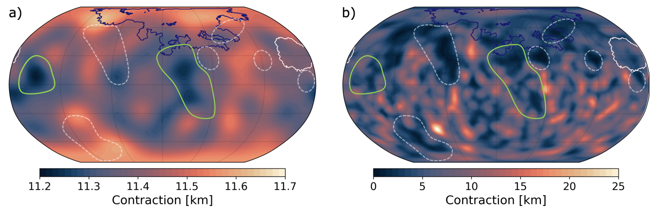
With our models, we are able to match the average global contraction estimates from observational constraints accounting for all tectonic landforms (>7 km; e.g., Byrne et al., 2014, Broquet & Andrews-Hanna, 2026), as well as a pattern of contraction dominated by surface temperature (Figure 2). While we can reproduce some regional patterns of low contraction, we are not able to replicate the large range of local contraction, as well as the regions that show no evidence of tectonic strain (Broquet & Andrews-Hanna, 2026). This implies that major processes, not captured in our geodynamics models, have affected Mercury’s contractional history. 

We show that planetary contraction is far from isotropic, which has implications for our understanding of Mercury’s tectonic record. More detailed comparisons of our planetary contraction estimates with those inferred from shortening landforms will provide important insights into the interior processes and cooling history of Mercury.

Figure 2: Comparison of a) our best-fit model contraction estimates since 3.8 Ga to b) contraction calculated from tectonic strain (Broquet & Andrews-Hanna, 2026). The Caloris basin (light pink) and a selected area of the smooth plains (dark blue) are outlined (Denevi et al., 2013). Green outlines show good agreements between model and observational estimates. White, dotted outlines represent low-contraction areas not explained by our model, which display high surface roughness (Nishiyama et al., submitted).

How to cite: Büttner, T., Broquet, A., Plesa, A.-C., Santangelo, S., Stark, A., and Hussmann, H.: Can Mercury’s heterogeneous tectonic record be explained by geodynamic models?, Europlanet Science Congress 2026, The Hague, The Netherlands, 7–11 Sep 2026, EPSC2026-1070, https://doi.org/10.5194/epsc2026-1070, 2026.

EPSC2026-1070

Download Close

Introduction

Mercury will soon be visited by the BepiColombo mission, whose scientific objectives span a wide range of topics in physics and planetary science. Investigating its interior and origin is crucial for understanding the formation and evolution of the Solar System. To this aim, the Mercury Orbiter Radio science Experiment (MORE) will enable the determination of the static gravity field and Mercury’s potential Love number k₂^[1], which quantifies the response of a planetary body’s gravity potential to tidal forcing.

In many cases, a static tide approximation is adopted, leading to the determination of a single k₂ value. For Mercury, previous geodetic studies have generally adopted this approximation, that effectively neglects any frequency dependence and phase lag in the tidal response. However, a more realistic description of planetary bodies would instead require viscoelastic rheological models, in which the material response depends on the frequency of the forcing^[4]. Since tidal forcing can be expressed as a Fourier sum of different tidal modes, each associated with a distinct frequency^[2], in this description the Love number emerges as a frequency-dependent quantity, k₂(ω_2mpq)^[3], acting on each tidal component according to its forcing frequency. 

For many Solar System bodies, especially those on low-eccentricity orbits and in a 1:1 spin-orbit resonance, the contribution of secondary modes is negligible compared with that of the mode associated with the orbital frequency. However, Mercury’s peculiar orbital and rotational dynamics characterized by its large eccentricity (e=0.2056) and 3:2 spin-orbit resonance, may provide a unique opportunity to measure the frequency-dependent dynamical Love number  k₂(ω_2mpq). Here, we explore the scientific return and the feasibility of measuring the dynamical Love number k₂ using future measurements from BepiColombo mission. The internal structure of Mercury is indeed widely debated^[5,6,8], and we suggest that the recovery of Mercury's frequency-dependent Love number would offer an opportunity to better understand its mantle relaxation timescales, over the range of periods characteristic of the tidal forcing.

Methods and Results

We first assess the expected accuracy of the Love number estimation by simulating range and Doppler measurements in Ka-band over the two-year extended orbital phase and processing them through a least-squares estimation to recover the spacecraft trajectory, gravity field, dynamical Love numbers, and rotational parameters. Once the accuracies are estimated, we generate a set of toy models and, using ALMA3^[7], we compute the Love number over the range of frequencies that compose the tidal forcing signal. These models span the range of interior architectures proposed in the current literature for Mercury, accounting for different polar moments of inertia, CMB radius, mantle configurations, and lithospheric rigiditis. They aim at providing a framework to assess whether the recovered dynamical Love number could discriminate between different interior scenarios.
Finally, our work shows that measurement of the dynamical Love number can significantly improve our understanding of Mercury’s mantle relaxation timescales, providing new and essential constraints on its internal structure. 

Acknowledments

A.C. and G. M. acknowledge support from the Italian Space Agency (2022-16-HH.1-2024)

Bibliography

[1] Luciano Iess, et al. Gravity, geodesy and fundamental physics with bepicolombo’s more investigation. Space Science Reviews, 217(1):21, 2021.

[2] William M. Kaula. Tidal dissipation by solid friction and the resulting orbital evolution. Reviews of geophysics, 2(4):661–685, 1964.

[3] Michael Efroimsky and Valeri V. Makarov. Tidal dissipation in a homogeneous spherical body. I. Methods. The Astrophysical Journal, 795(1):6, 2014.

[4] Sebastiano Padovan, et al. The tides of Mercury and possible implications for its interior structure. Journal of Geophysical Research: Planets, 119(4):850–866, 2014.

[5] Jean-Luc Margot, et al. Mercury’s Internal Structure. Cambridge Planetary Science. Cambridge University Press, 2018.

[6] Antonio Genova, et al. Geodesy, geophysics and fundamental physics investigations of the BepiColombo mission. Space Science Reviews, 217(2):31, 2021.

[7] Daniele Melini, Christelle Saliby, and Giorgio Spada. On computing viscoelastic Love numbers for general planetary models: the ALMA3 code. Geophysical Journal International, 231(3):1502–1517, 2022.

[8] Dunnigan, Abigail H., et al. Interior models of Mercury and conditions for iron snow formation in a Fe‐S‐Si core. Journal of Geophysical Research: Planets 131.4, 2026.

How to cite: Consorzi, A., Mitri, G., De Marchi, F., Zurria, A., Durante, D., Tartaglia, P., and Iess, L.: Mercury’s frequency-dependent k2 Love number from MORE: constraints on mantle relaxation timescales at tidal forcing frequencies, Europlanet Science Congress 2026, The Hague, The Netherlands, 7–11 Sep 2026, EPSC2026-563, https://doi.org/10.5194/epsc2026-563, 2026.

EPSC2026-563

Download Close

The BepiColombo Laser Altimeter (BELA) is a core scientific instrument of the BepiColombo mission for measuring Mercury’s global topographic characteristics and surface shape. Compared with the Mercury Laser Altimeter (MLA) onboard the MESSENGER spacecraft, BELA and MLA differ significantly in orbital configuration, spatial coverage, and observation geometry. As a result, the existing MLA laser altimetry products may not be directly suitable as comparison benchmarks or control references for subsequent BELA orbital observations. Therefore, it is necessary to establish a prior control method based on MLA data to support high-precision quality assessment, profile deviation diagnosis, and accuracy improvement for future BELA data.

Due to systematic errors related to ranging, timing, orbit determination, and pointing, MLA laser profiles often exhibit elevation inconsistencies at crossover locations. This study first uses the elevation differences at crossover as constraints to perform crossover adjustment and consistency correction of the MLA laser altimetry data, thereby producing an MLA dataset with improved internal consistency. On this basis, we propose an adjusted-MLA-driven partitioned prior-control and profile deviation diagnosis method to support future BELA laser altimetry applications. The adjusted MLA crossover network exhibits clear spatial variations in orbital coverage density, crossover density, and elevation-difference consistency, resulting in regionally variable prior-control quality. On this basis, we establish a spatially differentiated prior-confidence evaluation framework by integrating information on crossover density, interpolation stability within crossover neighborhoods, post-adjustment residual statistics, and local terrain complexity, through which the study area is divided into high-, medium-, and low-confidence regions. When a subsequent BELA laser profile passes through a corresponding region, the prior information of that partition can be directly invoked for targeted profile deviation diagnosis. In high-confidence regions, the adjusted MLA laser profiles are used as strong reference benchmarks to evaluate the consistency between BELA profiles and the existing MLA elevation reference, and to identify overall elevation offsets and long-wavelength along-track trend errors. In medium-confidence regions, the MLA control results provide weak constraints in the form of regional statistical ranges and error bounds, which are used to assess the degree of deviation of BELA profiles and to screen for anomalous residuals. In low-confidence regions, new BELA observations are used to reversely validate the existing control results.

The prior-control unit library constructed in this study can provide prior support for BELA profile quality assessment and error-source analysis after orbital insertion. It can also support rapid validation of early BELA data, subsequent global topographic recovery, and cross-mission joint laser altimetry applications.

How to cite: Yang, B., Xie, H., Liu, S., Xu, Q., Sun, Y., and Hou, Y.: Construction of partitioned prior-control units from crossover-adjusted MLA profiles for BELA applications, Europlanet Science Congress 2026, The Hague, The Netherlands, 7–11 Sep 2026, EPSC2026-395, https://doi.org/10.5194/epsc2026-395, 2026.

EPSC2026-395

Download Close

Introduction: Despite major advances from the MESSENGER mission, important questions remain regarding Mercury’s rotational state and internal structure. Independent analyses of Earth-based radar observations (Margot et al., 2007, 2012), radio tracking data (Mazarico et al., 2014; Verma and Margot, 2016; Genova et al., 2019; Konopliv et al., 2020), and laser altimetry (Stark et al., 2015; Bertone et al., 2021, Xiao et al., 2025) have yielded different estimates of Mercury's spin pole orientation. These orientation parameters can be combined with the gravity field under the assumption of the Cassini state to derive the polar moment of inertia C/MR² (Peale et al., 2002), widely used to constrain interior models (e.g. Genova et al., 2019; Goossens et al., 2022). However, measurements show that Mercury's spin pole deviates from the Cassini plane, suggesting that the exact Cassini state assumption is not fully consistent with observations. The observed offset thus represents an independent and meaningful constraint on Mercury's internal structure. MacPherson and Dumberry (2022) showed that the observed upper bound on the Cassini state offset implies a bulk mantle viscosity no smaller than approximately 10¹⁷ Pa s if a Maxwell rheology is assumed, a constraint that may be difficult to reconcile with the low mantle viscosities of 10¹⁶–10¹⁸ Pa s typically required to reproduce the observed k₂ values in the range 0.53–0.57 derived by Genova et al. (2019) and Konopliv et al. (2020). In this work, we incorporate the rotational model of MacPherson and Dumberry (2022) into a Markov Chain Monte Carlo (MCMC) framework to jointly use Mercury’s mass, 88-day libration amplitude, obliquity, Cassini state offset, and k₂ as observational constraints. This formulation replaces the moment of inertia of the planet, C/MR², derived under the Cassini state assumption, and the silicate-shell-to-planet moment of inertia, C_cr+m/C, with quantities directly tied to rotational and tidal measurements. We focus on the solutions of Genova et al. (2019) and Konopliv et al. (2020), which both provide k₂ estimates but differ significantly in their spin-pole orientation parameters, and assess the consistency between the geophysical observables and the corresponding interior models.

Methods: We develop a Bayesian inference framework for the interior structure inversion of Mercury based on a MCMC approach. The inversion jointly uses Mercury’s mass, obliquity, offset from the Cassini plane, libration amplitude, and tidal Love number k₂ as observational constraints for the planet. Mercury is modeled as a multi-layered body, with layer radii, densities, shear moduli, and viscosities treated as free parameters. These parameters are sampled iteratively using the Metropolis-Hastings algorithm, producing an ensemble of interior models consistent with the adopted prior distributions and observational uncertainties. After verifying the convergence of all chains, we compute the marginal posterior distributions of the model parameters, which constrain the range of internal structures consistent with the full set of geophysical observables.  

Mercury Interior Model Inversion: The internal structure of Mercury is constrained using geophysical parameters derived from MESSENGER mission data. In this work, we compare inferred interior structure models obtained from two sets of orientation parameters reflecting significantly different rotational states. The first set is from Genova et al. (2019), who estimated an obliquity of 1.968 ± 0.027 arcmin and a Cassini state offset of 0.004 ± 1.52 arcsec, placing Mercury nearly on the Cassini plane. The second set is from Konopliv et al. (2020), who report an obliquity of 2.04 ± 0.1 arcmin and an offset of 8.9 ± 4.49 arcsec, indicating a measurable departure from the exact Cassini state. Both studies also provide estimates of the tidal Love number k₂, obtaining values of 0.569 ± 0.025 and 0.53 ± 0.03, respectively. The 88-day libration amplitude is taken from Margot et al. (2012), who reported a forced libration of 38.5 ± 1.6 arcsec. Librations are modeled following the formulation of Van Hoolst et al. (2012), accounting for the effect of gravitational coupling with a solid inner core. Mercury's obliquity and spin-axis deviation from the Cassini plane are computed using the rotational model of MacPherson and Dumberry (2022). This model accounts for viscous and electromagnetic friction at the core-mantle boundary and inner core boundary, as well as deformations resulting from tidal forcing and differential rotation between internal layers.

Mercury is modeled as a four-layer body composed of a solid inner core, a fluid outer core, a mantle, and a crust. The radii of all layers are assumed as free parameters, while the mantle thickness is determined from the known planetary radius. The densities of all layers, the shear moduli, and viscosities of the solid regions are included as free parameters. Starting from a spherical description of the interior, the flattening of each internal interface is computed by imposing the observed surface flattening, gravitational equipotential surfaces at the inner- and outer-core boundaries, and consistency with the degree-2 gravity field coefficients C₂₀ and C₂₂.

Preliminary results suggest that the joint use of librations, obliquity, Cassini state offset, and k₂ as independent observational constraints reveals inconsistencies between the geophysical observables associated with the two rotational solutions. These inconsistencies are partly masked when the interior inversion relies only on the moment of inertia derivded under the Cassini state assumption.

How to cite: Ciambellini, M., Rivoldini, A., Van Hoolst, T., Gargiulo, A. M., and Genova, A.: Constraining Mercury’s interior structure by using rotational parameters in a Bayesian framework, Europlanet Science Congress 2026, The Hague, The Netherlands, 7–11 Sep 2026, EPSC2026-1323, https://doi.org/10.5194/epsc2026-1323, 2026.

EPSC2026-1323

Download Close

Introduction: Understanding the surface composition of Mercury remains one of the most challenging aspects related to the study of this planetary body. As of today, observations from the NASA MESSENGER mission show that most of Mercury’s surface does not exhibit distinctive absorption features in the visible and near-infrared range [1]. A notable exception is the presence of a 630 nm band, possibly coupled with a ~900-1000 nm inflection, associated with the enigmatic features known as hollows. Additionally, a feature at 830 nm was discovered in the relatively fresh material within the Praxiteles basin, including hollows in the early stage of their formation [2]. 

Hollows are a surface morphological expression unique to Mercury, consisting of bright and irregular flat-floored depressions and thought to form by loss of volatiles from the surface [3]. Indeed, their feature at 630 nm has been attributed to the presence of volatile sulfide and chloride species [4-6]. However, it has also been pointed out that low-iron mafic silicate minerals enriched in Cr, Ti and Ni could be partly responsible for the hollows’ spectral behavior [7]. The 830 nm feature is also suggested to be related to low-iron minerals [2]. Hence, hollows potentially represent a unique window on the planet’s extremely reducing crust. Given these premises, expanding on the range of investigated hollows is essential to study the extent of variability of their spectral features, providing constraints on their formation mechanism and on the nature of the bedrock on which they form. 

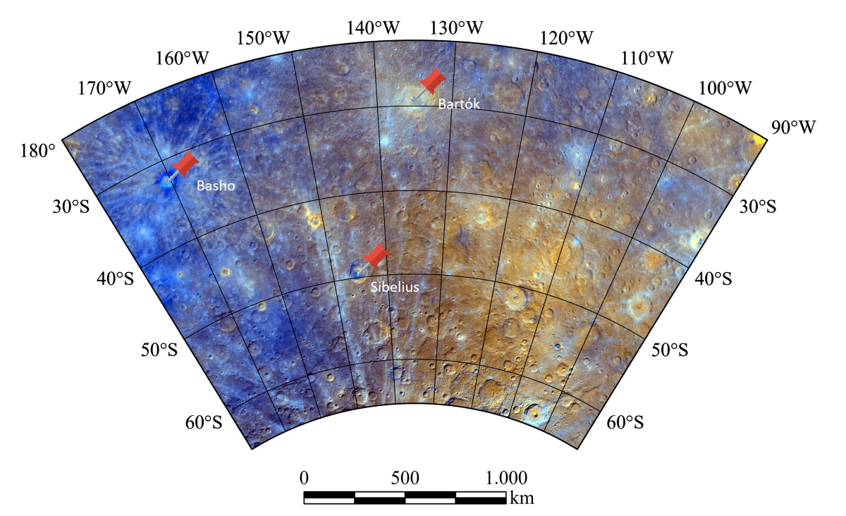
In this work we investigated the spectral variability of hollows in the Michelangelo quadrangle (H12, Figure 1) using unsupervised machine learning. Considering the current challenges of identifying spectral signatures on Mercury, such advanced methods can be particularly useful to identify patterns and subtle spectral changes. The selected region encompasses several areas where hollow fields are present. The Michelangelo quadrangle (lat. 22.5°S–65.0°S and lon. 180°E–270°E) has diverse terrains, offering a range of potential bedrock sources for hollow formation: morphologically, the area is dominated by intermediate plains, while intercrater plains are the second most widespread unit [8]; spectrally, the region is characterized by both dark-blue terrains and by bright reddish-yellow terrains (Figure 1).

Figure 1. MDIS enhanced mosaic of Michelangelo quadrangle. Selected areas for spectral analysis of hollows are pinpointed on the map.

Data and methods: Hollow fields were selected based on the global catalogs by [9, 10] and from the map of the Michelangelo quadrangle by [8]. This information was combined with the map by [11], which highlights the broad, shallow band near 600 nm that is observed in low reflectance materials (LRM) but often also found in hollow materials. Based on this, we identified large hollow fields with a strong 600 nm feature in Basho, Bartók, and Sibelius craters (Figure 1). 

For spectral analysis, we employed multispectral data (400-1000 nm) from the MESSENGER Mercury Dual Imaging System (MDIS) - WAC. EDR (Experiment Data Records) images were radiometrically and photometrically corrected following [12] and stacked to data cubes through the Integrated Software for Imagers and Spectrometers (ISIS). High-resolution MDIS-NAC images (panchromatic, 750 nm), radiometrically and photometrically corrected, are used for contextual and morphological analysis. MDIS-WAC data are clustered via unsupervised learning using a full covariance gaussian mixture model (GMM), a method which well suits spectral data analysis, being fast and capable of dealing with complex large datasets. 

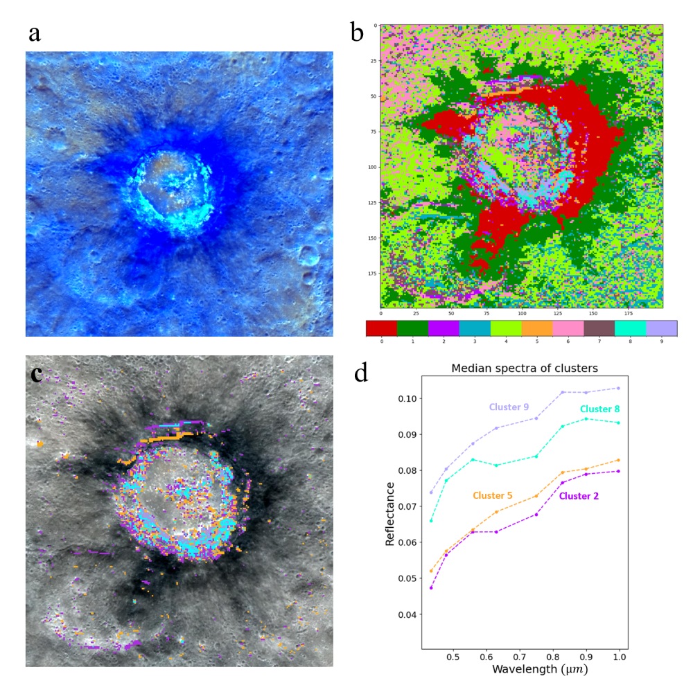
Results: We show results from Basho crater (Figure 2). The cluster analysis was performed on a portion of an 8 filter WAC image at 840 m/px resolution. Considering the color variability from the enhanced map (Figure 2a), 10 clusters were given as input to the algorithm (Figure 2b). Of these, 4 clusters correlate to areas with hollow fields and nearby terrains (clusters number 2, 5, 8, 9; Figure 2b and 2c). The average (median) spectral signatures of these clusters are shown in Figure 2d. 

Clusters 2 and 8 show a broad ~ 550-800 nm range absorption feature related to hollows with different average reflectance levels. Additionally, cluster 8 displays a deeper band in the 550-800 nm range, as well as an inflection towards 1000 nm. Clusters 5 and 9 do not show the 550-800 nm band, but highlight the presence of a shallow 900 nm band. Results from Bartòk, and Sibelius reveal a similar variability.

Figure 2.  (a) MDIS enhanced view of Basho crater. Hollows and surrounding materials appear in bright cyan colors; (b) spectral clusters obtained with a full covariance GMM; (c) clusters in (b) spatially correlating with hollows and surrounding materials; (d) median spectra of clusters from panel (c).

Summary and future perspectives: By means of unsupervised machine learning we provided evidence of high spectral variability among hollow-associated materials in the area of the Michelangelo quadrangle. Future characterization will include complementary analysis with spectral indices and correlation with morphology to better assess the origin and possible interpretation of the observed signatures. The results will represent an important pre-characterization of hollow materials in preparation for the observations by the SIMBIO-SYS/Visible Infrared Hyperspectral Imager Channel (VIHI) instrument onboard the ESA/JAXA BepiColombo mission. In particular, the Michelangelo quadrangle is scheduled to be imaged within the first six months of the primary mission phase, offering one of the earliest opportunities to directly compare new orbital hyperspectral observations with the spectral trends identified in this study.  

References: [1] Izenberg et al., 2014, Icarus, 228 (2014); [2] Galiano et al., 2026, Planet. Sci. J. 7, 27. [3] Blewett et al., 2011, Science, 333, 1856-1859; [4] Vilas et al., 2016, Geophys. Res. Lett., 43, 1450-1456. [5] Lucchetti et al., 2021, Icarus, 370, 114694; [6] Barraud et al., 2023, Science, 9(12), eadd6452; [7] Lucchetti et al., 2018, JGR: Planets, 123, 2365-2379; [8] Buoninfante et al., 2015, J. Maps, 21 (1); [9] De Toffoli et al., 2024, ESS, 11, 12; [10] Bickel et al., 2025, JGR: MLC, 2, e2024JH000431. [11] Klima et al., 2018, GRL, 45, 7. [12] Domingue et al., 2016, Icarus, 268, 172-203.

Acknowledgments: this study is supported by the ASI agreement n. 2024-18-HH.0

How to cite: Baschetti, B., Filacchione, G., Buoninfante, S., Carli, C., Galiano, A., Zambon, F., Munaretto, G., Tullo, A., Vergara Sassarini, N. A., Re, C., Tognon, G., Massironi, M., Giacomini, L., Galluzzi, V., Capaccioni, F., and Cremonese, G.: Spectral variability of hollows in the Michelangelo quadrangle of Mercury as revealed through unsupervised clustering methods., Europlanet Science Congress 2026, The Hague, The Netherlands, 7–11 Sep 2026, EPSC2026-790, https://doi.org/10.5194/epsc2026-790, 2026.

EPSC2026-790

Download Close

Introduction

On its cruise to Mercury, BepiColombo (ESA/JAXA) performed six flybys at the innermost planet. During the fifth flyby in December 2024, the onboard Mercury Radiometer and Thermal Infrared Spectrometer (MERTIS) [1,2] acquired the first spaceborne thermal infrared spectra of the planet (spectrometer wavelength range = 7-14 μm) [3]. These data are valuable because they provide new insights into Mercury’s surface and enable the MERTIS team to better prepare for BepiColombo’s orbit science phase starting in 2027. Furthermore, the flyby's unique geometry provides illumination and viewing conditions that will not be available during the main mission. This is especially important for adapting thermal models to Mercury's emission characteristics to retrieve thermophysical properties and emissivity spectra.

Preliminary results from the flyby indicate an overall spectrally homogeneous surface, though spotted with local variations [4]. Typically, these variations follow a lunar-like pattern in which fresh craters exhibit high visible brightness and bolometric albedo, leading to proportionally lower thermal infrared (TIR) radiance. However, we also identify anomalous regions where reduced visible radiance coincides with decreased TIR emission. This unexpected thermal behavior challenges standard thermophysical modeling, leading us to identify bolometric emissivity as a critical parameter in explaining these distinct regions.

Methods

Mercury’s rough surface leads to anisotropic thermal emission that cannot be adequately modeled by a simple blackbody assumption. We are currently investigating and comparing different thermal roughness models that utilize either bowl-shaped craters [5,6,7] or fractal surfaces [8,9]. In this work, we utilize the fractal roughness model of [9] to retrieve apparent emissivity maps. The three main model parameters are the bolometric directional-hemispherical albedo A_dh, the bolometric hemispherical emissivity ε_h, and surface roughness, characterized by the RMS slope θ. To highlight deviations in the thermal emission behavior, we fix A_dh = 0.08, derived from MESSENGER MDIS data [10]. We fit the remaining model parameters to the measured radiance assuming unit emissivity at the Christiansen feature. The apparent (unaccounted for spatially varying A_dh) spectral emissivity maps are computed by dividing the measured radiance by the model output (see Figure 1).

Figure 1: Measured (left) and modeled (right) radiance at 8.57 μm in orthographic projection on top of the MDIS WAC mosaic [10], center longitude = 180°.

Preliminary Results

Inverting the thermal model with Bayesian optimization yields a high surface roughness of θ ≈ 35°, consistent with lunar values (e.g. [5,9,11,12]) and a low bolometric emissivity of ε_h ≈ 0.75 – 0.85. The bolometric emissivity is lower compared to lunar values (ε_h ≈ 0.95 – 1.0). Bolometric emissivity represents the total spectral emissivity weighted across the blackbody emission curve. As Mercury’s high dayside temperatures shift this thermal emission peak to shorter wavelengths, it samples regions of lower spectral emissivity, driving down the overall ε_h (see Figure 2).

Figure 2: Simulated example silicate emissivity spectra (based on [14]) with different amounts of carbon and blackbody thermal emission at Hermean temperatures.

Figure 3 shows that the local emissivity variations appear nearly uniform across all observed wavelengths. Therefore, we focus on a single wavelength to characterize the variations. White arrows in Figure 4 highlight normal cases, where high reflectance in the visible spectrum corresponds to reduced thermal emission and thus reduced apparent emissivity. The dashed lines indicate thermal anomalies where this relationship does not hold. At Atget crater (A1 in Figure 4), reduced visible radiance coincides with decreased TIR emission, whereas Tolstoj basin (A2 in Figure 4) shows no comparable TIR response. These observations challenge standard thermophysical interpretations and instead point to variations in bolometric emissivity as the controlling factor. We investigated several possible causes of this behavior, including carbon, hypothesized to form LRM (Low Reflectance Material) [13], space weathering effects, and variations in grain size and roughness. Laboratory measurements and simulations show that adding carbon (graphite) to the mixture lowers the reflectance in the visible spectrum but has only a minimal effect on the spectral emissivity in the TIR. However, it leads to a significant increase in spectral emissivity in the 4-6 μm region (see Figure 2), thereby increasing the bolometric emissivity and decreasing thermal emission. These effects are nonlinear and might explain the different thermal anomalies.

Figure 3: Apparent emissivity maps at different wavelengths, colors scaled to enhance contrast. The spatial variations appear almost uniform across bands.

Figure 4: (Left) MDIS WAC enhanced color mosaic [10], projected to match the MERTIS observations. (Center) MERTIS apparent emissivity at 8.57 μm. (Right) MDIS WAC reflectance at 750 nm filtered to approximate the spatial resolution (≈ 30 km/pix) of MERTIS during the flyby. White arrows indicate the expected behavior, the dashed lines highlight thermal anomalies.

References

[1] Hiesinger, H., et al. 2010, Planet Space Sci. 58, 1-2, 144-165, https://doi.org/10.1016/j.pss.2008.09.019
[2] Hiesinger, H., et al. 2020, Space Sci. Rev., 216, 110
[3] Adeli, S., et al., 2025, LPSC #2501 (2025)
[4] Wohlfarth, K., et al. 2026, LPSC #1628 (2026)
[5] Jhoti, E. et al. 2026. Journal of Geophysical Research: Planets, 131, e2026JE009661. https://doi.org/10.1029/2026JE009661
[6] Powell, T., et al. 2025, LPSC #2317 (2025)
[7] Kührt, E. et al. 1992, Icarus, 96, 2, 213-218, https://doi.org/10.1016/0019-1035(92)90075-I
[8] Groussin, O. 2025, A&A, 694, A21, https://doi.org/10.1051/0004-6361/202452260
[9] Wohlfarth, K., et al. 2023, A&A, 674, A69, https://doi.org/10.1051/0004-6361/202245343
[10] B. W. Denevi et al. 2016, LPSC #1264 (2016).
[11] Bandfield, J.L et al. 2015, Icarus, 248, 357
[12] Rubanenko, L. et al. 2020, J. Geophys. Res. Planets, 125.
[13] Klima, R. L. et al. 2018, Geophysical Research Letters, 45, 2945–2953. https://doi.org/10.1002/2018GL077544
[14] RELAB Spectral Database, Brown University, 2014, https://sites.brown.edu/relab/

How to cite: Tenthoff, M., Wohlfarth, K., Knollenberg, J., Powell, T. M., Groussin, O., Kührt, E., Wöhler, C., Adeli, S., Barraud, O., Bauch, K. E., Benkhoff, J., Domaç, A., Greenhagen, B. T., Hamm, M., Helbert, J., Heyer, T., Hiesinger, H., Nishiyama, G., Pasckert, J. H., and Schmedemann, N. and the Hermean Emissivity and Thermophysics Working Group: MERTIS Reveals Thermal Anomalies on Mercury's Surface during BepiColombo’s Fifth Flyby, Europlanet Science Congress 2026, The Hague, The Netherlands, 7–11 Sep 2026, EPSC2026-907, https://doi.org/10.5194/epsc2026-907, 2026.

EPSC2026-907

Download Close

On December 1st, 2024, ESA/JAXA BepiColombo has become the 3rd spacecraft to observe the surface of Mercury, after Mariner 10’s flybys in 1974-75 and MESSENGER orbiting Mercury between 2011 and 2015. BepiColombo’s arrival is planned for November, 2026 - an 8 years journey which includes six flybys to guide the spacecraft into the orbit. The 5th flyby geometry has offered an exceptional and first-time opportunity for the MErcury Radiometer and Thermal Infrared Spectrometer (MERTIS) to observe the planet’s surface through its Space Port. MERTIS is composed of a spectrometer (TIS) operating in the spectral range of 7-14 µm and a radiometer (TIR) with two channels at 8-14 µm and 7-40 µm [1]. The 5th flyby has marked the first time that Mercury’s surface has been observed in the spectrally resolved mid-IR range by a spacecraft [2]. This spectral range allows to better understand Mercury’s surface composition, as it is sensitive to Si–O stretching vibrations and allows identification of feldspars, pyroxenes, olivines, sulfides, volcanic glasses, silica-rich materials, potentially graphite-bearing or reduced materials. The intrinsic lack of diagnostic absorption features in Mercury’s VNIR spectra has historically (e,g, MESSENGER mission data) masked the planet’s true mineralogical diversity .

This work focuses on (1) mapping the surface variations observed within the 5th flyby coverage of the MERTIS instrument in the mid-IR range; (2) investigating correlations with previously reported surface features and geological units; (3) studying the global (within the 5th flyby coverage) effect of various surface- and temperature-dependent parameters on the MERTIS mid-IR signal variations.

Data calibration: The data acquisition and processing architecture of the MERTIS instrument is described in detail in [3]. The MERTIS instrument is designed to observe at Mercury through its planet port. The Space Port is intended as a calibration target with „no emission”, observing deep space [1]. The MERTIS planet port view was characterized in the laboratory during a radiometric calibration campaign under space-like thermal-vacuum conditions [3, 4]. Since launch, there have been observation campaigns for the Moon [5] and Venus [6]. The instrument had to be reprogrammed to observe the targets through the Space Port, which had not been intended for scientific observations. The current calibration of the 5th flyby data of Mercury is based on the calibration methods developed during the cruise alongside Venus and the Moon.

Preliminary results and discussion: Impact basins and complex craters serve as primary thermal and compositional benchmarks within the radiance dataset of the 5th flyby. This is most likely due to the strong temperature differences they exhibit compared to their surroundings, which are likely a result of differences in composition and/or degree of space-weathering. One example is the Tolstoj basin under study in [7]. A larger dataset of central peaks is currently under investigation [8]. The impact crater Bashō is another location where we observe anomalies in the mid-IR data. Similarly, MESSENGER visible images show that Bashō crater exhibits both dark and bright material. Other anomalous regions were observed where reduced visible radiance (in MESSENGER data) coincides with decreased thermal IR emission of MERTIS data [9, 10].

The Christiansen Feature (CF) is one of the most important spectral parameters in the mid-IR range. The CF position shifts with various factors such as silica content, glass content, grain size, temperature, and bulk composition, e.g., felsic materials show a CF at shorter wavelengths whereas mafic/ultramafic materials tend to have a CF at longer wavelengths.

The mean CF value of all MERTIS observation of the 5^th BepiColombo flyby lies approximately between 8.2 and 9.0 μm, which implies rather mafic assemblages, low silica content and abundant pyroxene/olivine-like materials[1] . Glassy volcanic material may also be present on the surface.

Next steps:

• Analysis of CF shift as a proxy to Mercury’s bulk composition
• Refinement of the CF retrieval from the flyby dataset
• Comparison with visible and NIR data of MESSENGER
• Laboratory work and comparison with analogue samples for more detail, see [11, 12, 13, 14].

Reference

[1] Hiesinger et al., Earth and Planetary Sci. L., 2008. [2] Hiesinger et al., LPSC, 2025. [3] D’Amore, M. et al, Infr. Remote Sens. Instr, 2018. [4] Walter, I., et al., Infrared Remote Sensing and Instr, XXI, 2013. [5] Barraud et al. SPIE 2024. [6] Helbert et al. Nature Comm. 2023. [7] D’Amore et al., LPSC 2025. [8] Pasckert et al., LPSC 2025. [9] Wohlfarth et al., LPSC 2026. [10] Tenthoff et al., EPSC 2026. [11] Maturilli et al., LPSC 2025. [12] Morlok et al., EPSC-DPS 2025. [13] Van den Neucker et al., LPSC 2025 [14] Verma et al., EPSC 2026

How to cite: Adeli, S., Helbert, J., Maturilli, A., Wöhler, C., and Hiesinger, H. and the MERTIS Science Team: BepiColombo's 5th Flyby: MERTIS Observations of Mercury's Surface Variations – Preliminary results, Europlanet Science Congress 2026, The Hague, The Netherlands, 7–11 Sep 2026, EPSC2026-1194, https://doi.org/10.5194/epsc2026-1194, 2026.

EPSC2026-1194

Download Close

Tectonism, fault mechanics and global contraction are major areas of geologic research on Mercury. The Spectrometer and Imagers for MPO BepiColombo Integrated Observatory System (SIMBIO-SYS) instrument suite onboard BepiColombo has three channel observation capabilities, differing in resolution, observation area and frequency, which are poised to offer new insights to our understanding of mercurian tectonics. These channels include 1. the High-Resolution Imaging Channel (HRIC) which provides target oriented observations with panchromatic and color filters, 2. The Visibile-Infrared Hyperspectral Imager (VIHI) which provides global mapping, as well as higher resolution target oriented observations and 3. The Stereo Imaging Channel (STC) which provides global mapping and target oriented observations (Galluzzi et al., 2025). The relationships between local, regional and global tectonics, and the influence of crustal structure and thickness remain major aspects of tectonism on Mercury that are not fully understood (e.g. Galluzzi et al., 2019; Klimczak et al., 2025; Schmidt et al., 2026). These tectonic aspects are incorporated into the scientific objectives specific to SIMBIO-SYS,
which in tandem with gravity data from the Mercury Orbiter Radio Science Expirement (MORE) can be thoroughly addressed by BepiColombo.

There are upwards of 250 planned targets of tectonic interest specific to SIMBIO-SYS. These targets include structures and landforms such as thrusts (or rupes), "fresh" faults (e.g. Watters 2016), graben (e.g. Man et al., 2023), depressions and geological unit contacts, as well as various terrains. Further still are many other targets associated to volcanism and basins which have a shared scientific rationale to tectonism. The significance that these landforms have to our understanding of the geologic history of Mercury cannot be emphasized enough. Considering also that Mercury represents a planetary body that had extensive tectonic activity in its past, yet remained a stagnant lid, data from these targets has the potential to further our understanding of planet evolution and the Solar System in general.

In an effort to convey the scientific contribution that SIMBIO-SYS is prepared to deliver, here we discuss the objectives and importance of these targets, and present specific examples and how each plays a role in addressing scientific questions. The complex structural geology of Mercury stands to demonstrate to us many aspects of fault mechanics and planet evolution that can often go under appreciated when studying the geology of Earth. Thus, the planned targets of tectonic interest captured by SIMBIO-SYS represent a great opportunity to geological science.

Acknowledgments:

We gratefully acknowledge funding from the Italian Space Agency (ASI) under ASI-INAF agreement 2024-18-HH.0.

References:

Galluzzi, V., Palumbo, P., Capaccioni, F., Re, C., Filacchione, G., Cremonese, G., Agostini, L., Tubiana, C., Tullo, A., Zusi, M., Simioni, E., Doressoundiram, A., & Vincendon, M. (2025). BC-SIM-TN-017 SIMBIO-SYS Target-Oriented Observation Strategies (1.0). Zenodo. https://doi.org/10.5281/zenodo.15880226

Galluzzi, V., Ferranti, L., Massironi, M., Giacomini, L., Guzzetta, L., & Palumbo, P. (2019). Structural analysis of the Victoria quadrangle fault systems on Mercury: Timing, geometries, kinematics, and relationship with the high‐Mg region. Journal of Geophysical Research: Planets, 124(10), 2543-2562. https://doi.org/10.1029/2019JE005953

Klimczak, C., Crane, K. T., & Byrne, P. K. (2025). Mercury has multiple, superposed global tectonic patterns. Earth and Planetary Science Letters, 658, 119331. https://doi.org/10.1016/j.epsl.2025.119331

Man, B., Rothery, D. A., Balme, M. R., Conway, S. J., & Wright, J. (2023). Widespread small grabens consistent with recent tectonism on Mercury. Nature Geoscience, 16(10), 856-862. https://doi.org/10.1038/s41561-023-01281-5

Schmidt, G., Galluzzi, V., Sepe, A., Buoninfante, S., De Toffoli, B., Ferranti, L., & Palumbo, P. (2026). Origin of the bulge topography within Caloris basin, Mercury. Journal of Geophysical Research: Planets, 131(2), e2025JE009233. https://doi.org/10.1029/2025JE009233

Watters, T. R., Daud, K., Banks, M. E., Selvans, M. M., Chapman, C. R., & Ernst, C. M. (2016). Recent tectonic activity on Mercury revealed by small thrust fault scarps. Nature Geoscience, 9(10), 743-747. https://doi.org/10.1038/ngeo2814

How to cite: Schmidt, G. W., Galluzzi, V., Vergara, N. A., Buoninfante, S., Sepe, A., and Palumbo, P.: Structural targets of the SIMBIO-SYS instrument suite of BepiColombo: Objectives, categorization and tectonic signficance, Europlanet Science Congress 2026, The Hague, The Netherlands, 7–11 Sep 2026, EPSC2026-1163, https://doi.org/10.5194/epsc2026-1163, 2026.

EPSC2026-1163

Download Close

Towards Automated Identification and Characterization of Impact Craters on Mercury for Future BepiColombo BELA Observations

   Impact craters preserve key information about the geological evolution, surface age, and crustal structure of planetary bodies, making their identification and characterization an important objective in planetary remote sensing. On Mercury, interpretation of crater morphology is complicated by widespread volcanic resurfacing and modification, which can embay crater rims, infill interiors, and obscure older basin structures (Du et al., 2020; Bertoli et al., 2024; Golder et al., 2025). Laser altimetry from the MESSENGER Mercury Laser Altimeter (MLA) has provided the first detailed topographic view of Mercury’s northern hemisphere (Zuber et al., 2012) and enabled quantitative investigation of crater and basin morphology.

   Building on previous morphometric studies of Mercurian craters (Susorney et al., 2016) and our earlier work using RANSAC-based surface fitting and geomorphological analysis of laser-altimetry point clouds (Arghavanian et al., 2024; Arghavanian et al., 2025), this study investigates how crater-related topographic signatures can be identified directly from MLA-derived digital elevation models and point clouds. The analysis focuses on cross-sectional geometry (Arghavanian & Leloglu, 2024) e.g. diameter, D/H, curvature, elevation residuals, and roughness (Nishiyama et al., 2026) characteristics as diagnostic indicators for distinguishing large crater (>10 km) (Herrick et al., 2018) structures from surrounding terrain and for evaluating possible volcanic overprinting.

   The aim is to determine which topographic parameters are most effective for recognizing impact-crater morphology in Mercury altimetry data, and to establish a framework for identifying craters that may be especially suitable for future compositional and mineralogical investigation. In this way, crater detection is treated not only as a geomorphological problem, but also as a step toward identifying impact structures that may reveal distinctive subsurface materials or compositionally unusual units. Also, we are optimistic to automate the process potentially by combining these geomorphological features with machine-learning–based methods. This framework is intended as a preparatory step for application to higher-resolution observations from the BepiColombo Laser Altimeter (BELA) (Thomas et al., 2021), which will provide new opportunities to refine the identification and characterization of complex impact craters and to assess their relationships with volcanic resurfacing, composition, and other surface processes.

References

Azar Arghavanian, Oliver Stenzel, Martin Hilchenbach, 2024, Smooth Hermean surface extraction by Region Growing from MESSENGER Laser Altimeter Data, EPSC2024, Berlin, Germany.

Azar Arghavanian, Oliver Stenzel, Martin Hilchenbach, 2025, Hermean curvature-based geomorphic feature classification using Laser Altimetry data, EPSC2025, Helsinki, Finland.

Azar Arghavanian, Uğur Murat Leloğlu. 2024, Channel detection and tracking from LiDAR data in complicated terrain, Journal of Environmental modeling and software. Vol:171.

Silvia Bertoli, Alice Lucchetti, Maurizio Pajola, Elena Martellato, Matteo Massironi, Pamela Cambianica, Emanuele Simioni & Gabriele Cremonese, 2024, Geomorphology of craters located at Mercury’s north pole, Journal of Maps, Volume 20, Issue 1.

J Du, MA Wieczorek, W Fa, 2020, Thickness of lava flows within the northern smooth plains on Mercury as estimated by partially buried craters, Geophysical Research Letters, Wiley Online Library.

KB Golder, BJ Thomson, LR Ostrach, DM Burr, JP Emery, H Hiesinger, 2025, Source (s) of the Smooth Caloris Exterior Plains on Mercury: Mapping, Remote Analyses, and Scenarios for Future Testing with BepiColombo Data, Remote Sens. 2026, 18(1), 19.

R. Herrick, E. M. Bateman, W. G. Crumpacker, D. Bates, 2018, Observations From a Global Database of Impact Craters on Mercury With Diameters Greater than 5 km, Journal of Geophysical Research: Planets, 123, 2089–2109.

Nishiyama, F. Preusker, A. Broquet, A. Stark, H. Hussmann, E. Hauber, and N. Tosi, 2026, First Global Map of Mercury’s Surface Roughness Down to Kilometric Baselines: Implications for the Planet’s Geologic Evolution, Planet. Sci. J. 7, 59.

HCM Susorney, OS Barnouin, CM Ernst, CL Johnson, 2016, Morphometry of impact craters on Mercury from MESSENGER altimetry and imaging, Icarus, Volume 271, June 2016, Pages 180-193.

Thomas, H. Hussmann, T. Spohn, L. M. Lara, U. Christensen, M. Affolter, T. Bandy, T. Beck, S. Chakraborty, U. Geissbuehler, M. Gerber, K. Ghose, J. Gouman, S. Hosseini Arani, K. Kuske, A. Peteut, D. Piazza, M. Rieder, A. Servonet, C. Althaus, T. Behnke, K. Gwinner, C. Hüttig, R. Kallenbach, A. Lichopoj, K. Lingenauber, H.-G. Lötzke, F. Lüdicke, H. Michaelis, J. Oberst, R. Schrödter, A. Stark, G. Steinbrügge, S. del Togno, K. Wickhusen, J. M. Castro, M. Herranz, J. Rodrigo, H. Perplies, T. Weigel, S. Schulze-Walewski, S. Blum, A. Casciello, E. Rugi-Grond, W. Coppoolse, M. Rech, K. Weidlich, T. Leikert, R. Henkelmann, B. Trefzger & B. Metz, The BepiColombo Laser Altimeter, 2021, Space Science Reviews, Volume 217, article number 25.

Zuber, David E. Smith, Roger J. Phillips, Sean C. Solomon, Gregory A. Neumann, Steven A. Hauck II, Stanton J. Peale, Olivier S. Barnouin, James W. Head, Catherine L. Johnson, Frank G. Lemoine, Erwan Mazarico, Xiaoli Sun, Mark H. Torrence, Andrew M. Freed, Christian Klimczak, Jean-Luc Margot, Jürgen Oberst, Mark E. Perry, Ralph L. McNutt Jr., Jeffrey A. Balcerski, Nathalie Michel, Matthieu J. Talpe, Di Yang, 2012, Topography of the Northern Hemisphere of Mercury from MESSENGER Laser Altimetry Maria, Science 336, 217.

How to cite: Arghavanian, A., Stenzel, O., Renggli, C., Stark, A., Oberst, J., and Broquet, A.: Towards Automated Identification and Characterization of Impact Craters on Mercury for Future BepiColombo BELA Observations, Europlanet Science Congress 2026, The Hague, The Netherlands, 7–11 Sep 2026, EPSC2026-1132, https://doi.org/10.5194/epsc2026-1132, 2026.

EPSC2026-1132

Download Close

Introduction

Explosive volcanism produces diverse pyroclastic landforms, including scoria cones, which on Earth make up ~90% of subaerial volcanoes and form during Strombolian eruptions as steep edifices with slopes near the angle of repose (~30°). Similar features occur on Mars and the Moon but are less common and morphometrically distinct; Martian cones are broader with gentler slopes due to enhanced pyroclast dispersal [1,2].

On Mercury, such edifices were long thought absent, with explosive volcanism inferred mainly from diffuse deposits around irregular vents, consistent with models predicting wide dispersal under low gravity and near-vacuum conditions [3]. Two small candidate cones—the ~1.1 km Heaney cone and ~1.7 km NW Caloris cone—have been tentatively identified, but their origin remained uncertain [4].

Here, we identify a larger, breached pitted cone in NE Caloris Planitia (Fig. 1) and present the first morphometric analysis of all three structures using a new global high-resolution DTM. Their morphology is consistent with scoria cones, with the NE Caloris cone providing the strongest evidence.

Figure 1: (a) Physiographic overview of northeastern Caloris Planitia with the new 222 m/pixel DTM overlaid on the MDIS high-incidence global mosaic; key landforms are indicated (see legend). Black box outlines the location of Fig. 1b. (b) Slope map from the same DTM over the low-incidence MDIS mosaic. Dashed lines A–A′ and B–B′ mark the elevation and slope profiles shown on the right.

Methods

We analyzed MESSENGER topographic and image data, including a new global ~222 m/pixel stereo-DTM and derived slope maps. Previously published stereo-DTMs (DLR) were complemented with new quadrangles to produce a merged global model [5]. The DTM was combined with MDIS mosaics (166 m/pixel) and enhanced color data.

Our measurements (Table 1) included basal diameter, height, flank slopes, and volume, and assessed summit morphology and breach geometry using approaches comparable to terrestrial and Martian cone studies [2].

Results

The NE Caloris landform is a conical mountain with a breached flank and partially preserved summit, located ~60 km from the edge of Caloris Planitia within smooth plains and near vents, lobate scarps, and hollows. The NE Caloris cone is significantly larger than the Heaney and NW Caloris cones, with an average diameter of ~16.5 km and relief of ~1 km, yielding a volume of ~70–75 km³ (vs. ~15–20 km³ for the smaller cones) (Fig. 2). The central depression is unusually large (~6 km in diameter and ~0.7 km deep; ~35% of cone diameter). Flank slopes reach up to ~16°, well below the angle of repose (~30°), but comparable to or slightly lower than values reported for smaller cones (~13–19°). Compared to the two smaller, quasi-circular cones, the NE Caloris cone shows pronounced asymmetry and a breached flank. The northern summit of the NE Caloris cone hosts a ~2 km-wide light-blue anomaly associated with an irregular depression.

Figure 2: Perspective views of the NE Caloris cone (top) and the smaller Heaney and NW Caloris cones (center, bottom [4]), shown with enhanced color over the high-incidence MDIS mosaic and 6× vertically exaggerated elevation from the 222 m/pixel global DTM. The white arrow marks a small irregular depression with a light-blue anomaly on the NE Caloris cone summit.

Table 1: Comparison of morphometric and geographic parameters of the three pitted cones discussed here. 

Discussion

Opposite a volcanic edifice interpretation, we consider two alternative origins for the breached cone-like landform on NE Caloris Planitia:

Impact origin (degraded/ghost crater): Although Mercury hosts irregular, discontinuous craters, these typically have much lower rims than the observed cone. Even fresh craters of similar size have rims less than half as high. Ghost craters may appear breached, but their interiors are flat and level with surrounding plains, unlike the cone’s sloping floor ~200 m above the plains.

Caloris inner ring remnant: The cone has comparable relief and radial position to nearby inner ring massifs, but is less rugged and uniquely hosts a non-circular, non–bowl-shaped central depression. This feature is unlike impact craters or vents elsewhere in the region, with the vents typically lying  below surrounding plains and occurring adjacent to, not within, massifs.

We therefore favor an origin as a volcanic construct. Compared to the smaller, more symmetric Heaney and NW Caloris cones, the NE Caloris cone is larger, elongate, and breached, suggesting a higher eruptive volume, more complex evolution associated with flank instability (possibly caused by different lava rheologies), and/or structural control (Fig. 2). The small depression and light-blue anomaly on its northern summit may represent an early-stage hollow formed by volatile loss within the cone. All three mercurian cones discussed here occur near lobate scarps and hollows, suggesting structural control and the potential for volatile-enriched magmas. 

The cone’s size, asymmetry, and lack of visible lava flows supports an explosive emplacement scenario, possibly ballistic scoria deposition. This would be the largest scoria cone in the Solar System implying sustained, high-volume magma supply at low ejection speeds, which is unexpected under current models that predict widespread pyroclast dispersal on Mercury and not steep, kilometer-scale cones. On the Moon and Mars, diameters and reliefs of scoria cone-like landforms (e.g., Marius Hills and Ulysses Colles) reach ~40–70% of the NE Caloris cone values, while only ambiguous, less conical examples (e.g., the lunar Rümker or Gardner domes) achieve them [8,9]. On Earth, dimensions comparable to the NE Caloris cone are only achieved by stratovolcanoes breached by lateral eruptions, e.g., Mount St. Helens. For all three discussed cones, better DTMs, images, and hyperspectral data by BepiColombo will help to distinguish between basaltic or more evolved lavas and refine flank slopes, dimensions of central depressions, existences of associated lava flows, and the nature the potential hollow.  

References

[1] Brož et al., 2014, EPSL 406 [2] Brož et al., 2015, JGR-Planets 120 [3] Brož et al., 2018. GRL 45 [4] Wright et al., 2018, JGR-Planets 123 [5] Bernhardt et al., 2025, EPSC 2108 [6] Jozwiak, et al., 2025, LPSC 2193 [7] Bickel et al., 2025, JGR: Machine Learning and Computation 1. [8] Yin et al., 2025, JGR-Planets 129. [9] Brož et al., 2020, J. Volc. Geotherm. Res. 409

How to cite: Bernhardt, H. and Brož, P.: A breached cone-like mountain on Caloris Planitia, Mercury: A candidate scoria cone?, Europlanet Science Congress 2026, The Hague, The Netherlands, 7–11 Sep 2026, EPSC2026-31, https://doi.org/10.5194/epsc2026-31, 2026.

EPSC2026-31

Download Close

Mercury’s radar-bright polar deposits provide some of the strongest evidence for volatile accumulation on the innermost planet. Ground-based radar observations first identified highly reflective features associated with permanently shadowed regions, and MESSENGER later confirmed that many of these cold traps host water ice and other volatile-bearing materials. However, while recent work has shown that Mercury’s north polar deposits are heterogeneous at local scales, a comparable analysis of the south polar deposits has remained limited by the quality of available topographic, illumination, thermal, and radar data.

Here we present ongoing work focused on a selected set of Mercury’s south polar craters, combining newly recovered Arecibo S-band radar datasets with refined and enhanced local digital elevation models derived from MESSENGER MDIS NAC images. A key component of this effort is the recovery of individual same-circular and opposite-circular polarization images, enabling an analogous  analysis to recent north-polar work in which the two polarizations were used independently to characterize radar-bright deposits, scattering behavior, and local-scale heterogeneity. Additionally, high-resolution DEMs can now be used to measure the local radar incidence angle, allowing for radar scattering modeling that can be used to further constrain the properties of the deposits. 

A major challenge is the lack of MESSENGER altimetry at southern latitudes, leaving many scientifically important areas, including permanently shadowed regions, poorly sampled or unsampled. Rather than relying on simple interpolation, which can produce unrealistic crater morphologies, we apply inpainting techniques to recover plausible local topography while preserving consistency with the surrounding terrain. These enhanced DEMs support modeling of illumination, radar viewing geometry, and thermal environments, allowing us to examine how radar-bright deposits relate to local topography, incidence geometry, shadowing, and predicted temperatures, and to assess whether south polar deposits show spatial patterns comparable to those identified in the north.

This work also provides a timely framework for the BepiColombo era. The refined DEMs, recovered Arecibo radar products, and combined radar–illumination–thermal analysis developed here can provide local context for future BepiColombo observations of Mercury’s south polar cold traps. New BepiColombo measurements will also offer an opportunity to test, refine, and extend these methods, enabling more detailed characterization of Mercury’s polar volatile inventory and its relationship to surface geology, thermal environment, and volatile delivery or preservation processes.

How to cite: Bertone, S., Rivera-Valentín, E. G., Nolan, M. C., Meyer, H. M., Mazarico, E., Siegler, M., Martinez Camacho, J. M., and Chabot, N. L.: Characterizing Mercury’s South Polar Volatile Deposits with Arecibo Radar and Enhanced Topography, Europlanet Science Congress 2026, The Hague, The Netherlands, 7–11 Sep 2026, EPSC2026-571, https://doi.org/10.5194/epsc2026-571, 2026.

EPSC2026-571

Download Close

Mercury's lack of atmosphere allows magnetospheric and solar wind plasma direct access to the surface through precipitation, altering the surface and plasma composition. In this way, its space plasma environment interactions resemble that of the Moon. Lunar measurements show that such exposed surfaces are subject to electrostatic charging, where photoelectrons generated on the dayside creating a positive potential of a few V, while electron transport to the nightside induces a negative surface potential up to -100s V. Given Mercury's similar surface properties and long diurnal cycle, we expect a similar pattern in surface potential; indeed, the nightside potential is likely even more negative at Mercury than at the Moon due to high energy electron precipitation.

Lunar Prospector electron reflectrometry data indicates that this surface potential can be estimated remotely from pitch angle distributions of reflected particles, as the potential adds an energy-dependent term to the particle loss cone [1]. For positively charged ions and a negative surface potential, the size of the upward loss cone becomes inversely proportional to ion energy and can include all pitch angles < 90 degrees for sufficiently negative potentials. Thus, this effect has important implications for the ability of Mercury's magnetic field to trap particles on the nightside. We examine nightside pitch angle distributions from the Miniature Ion Precipitation Analyzer (MIPA) in the SERENA package from BepiColombo's second Mercury flyby for evidence of this loss cone energy dependence and find a noticeably visible effect for upward-going ions. Lunar surface potential analysis shows a strong dependence on electron temperature [2], so we use Mercury Electron Analyzer (MEA) electron temperature measurements from MFB2 [3] as a basis for fitting the loss cone and find good agreement with the MIPA data. This case study shows that estimation of surface potential from ion measurements is indeed possible, and promises interesting results to come from the BepiColombo orbital phase.

[1] Halekas, J. S., G. T. Delory, R. P. Lin, T. J. Stubbs, and W. M. Farrell. “Lunar Prospector Observations of the Electrostatic Potential of the Lunar Surface and Its Response to Incident Currents.” JGR: Space Physics 113, no. A9 (2008). https://doi.org/10.1029/2008JA013194.
[2] Stubbs, T. J., W. M. Farrell, J. S. Halekas, et al. “Dependence of Lunar Surface Charging on Solar Wind Plasma Conditions and Solar Irradiation.” P&SS 90 (January 2014): 10–27. https://doi.org/10.1016/j.pss.2013.07.008.
[3] Rojo, M., N. André, S. Aizawa, et al. “Structure and Dynamics of the Hermean Magnetosphere Revealed by Electron Observations from the Mercury Electron Analyzer after the First Three Mercury Flybys of BepiColombo.” A&A 687 (July 2024): A243. https://doi.org/10.1051/0004-6361/202449450.

How to cite: Williamson, H., Barabash, S., Rabia, J., Maynadie, T., Nilsson, H., Wieser, M., Futaana, Y., Rojo, M., and Milillo, A. and the MPO/SERENA team: The effect of surface potential on reflected ions at Mercury observed by BepiColombo SERENA/MIPA, Europlanet Science Congress 2026, The Hague, The Netherlands, 7–11 Sep 2026, EPSC2026-957, https://doi.org/10.5194/epsc2026-957, 2026.

EPSC2026-957

Download Close

The northern polar cap region of Mercury remains poorly explored, as the MESSENGER orbits were close to the surface. Moreover, this region appears to be
populated by tenuous plasma. The northern polar cap of Mercury was crossed twice during the 4th and 6th flybys of BepiColombo. The Mercury Electron Ana-
lyzer onboard BepiColombo allowed the probing of low-energy electrons for the first time in this region since the third flyby of Mariner 10. We show that the
northern polar cap is populated with dense and cold electrons. Simultaneously, the four ion sensors did not detect any particles. This lack of detection suggests the presence of very cold ions of exospheric origin. Such a measurement challenges current models of Mercury’s exosphere and could be compatible with a closure of Region 1 field aligned currents above the surface.

How to cite: Rojo, M., Dandouras, I., Aizawa, S., Dewey, R., Raines, J., Liu, Z.-Y., Le Liboux, T., Coustillet, C., Gonnet, A., Hadid, L., Harada, Y., Varsani, A., Williamson, H., Millilo, A., André, N., Saito, Y., and Murakami, G.: Evidence of a cold and dense plasma in the northern polar cap of Mercury, Europlanet Science Congress 2026, The Hague, The Netherlands, 7–11 Sep 2026, EPSC2026-896, https://doi.org/10.5194/epsc2026-896, 2026.

EPSC2026-896

Download Close

Even though it is the closest planet to the Sun, Mercury’s polar craters harbor large volatile deposits [1]. Observations of radar brightness [2], neutron absorption [3], and optical reflection [4] have led to the conclusion that the deposits are largely made up of water ice. Ultimately, a total water ice mass of 10¹³ – 10¹⁵ kg has been estimated [3].

Due to the low number of craters on the icy surfaces, it has been suggested that the ice has been deposited in the past few 100 million years [4], for example by a single cometary impact [5]. However, recent analysis of the ages of ice-filled craters indicates a significant correlation of crater age and water ice amount [6]. Such a behavior would rather point to a contribution from a steadily ongoing process. Previous work has discussed dust impacts and solar wind delivery as potential sources [7, 8]. Jones et al. [8] developed a model to quantify the accumulation of water in Mercury’s permanently shadowed regions (PSRs) following solar-wind H⁺ implantation. They estimate a small contribution on the order of 10¹³ kg to today’s deposits over the past billion years, assuming identical delivery rates as today.

However, observations of other stars have allowed us to constrain the behavior of the younger Sun and it has been established that it was much more active in the past. In particular, the mass loss rate via solar wind emission was orders of magnitude higher [9], which potentially provides a much-increased source of solar-wind implanted water. At the same time, the Sun’s Lyman alpha emission was much brighter [10], which increases the H₂O photodissociation rate and limits the efficiency of migration into Mercury’s PSRs. Several studies have also suggested that Mercury’s dynamo history has evolved significantly in the past, likely requiring a much stronger early dynamo to explain today’s remanent surface magnetization [11].

In this study, we aim to quantify the potential solar wind contribution to Mercury’s H₂O deposits by accounting for these different aspects. We perform hybrid simulations using the Amitis code [12] for a more intense young solar wind, considering a range of different dynamo strengths. Based on the results of solar wind H⁺ implantation, we calculate rates of water delivery into Mercury’s PSRs by accounting for the increased Lyman alpha strength in the past (up to a factor of 3).

When calculating the estimated total water amount accumulated over the past 3.7 billion years, we find that the result significantly depends on the assumptions regarding Mercury’s dynamo history. A gradual decrease of dynamo strength to today’s value typically leads to similar estimates as the original calculation from Jones et al. (2020) of a minor contribution of 10¹³ kg. However, if there were extensive time periods with a dynamo comparable to today’s strength or no dynamo at all, the calculated water deposits increase up to several 10¹⁴ kg, which would represent an important contribution to today’s ice deposits.

Our study thus further supports that solar wind implantation is a possible source of water ice in Mercury’s PSRs. The planet’s volatile deposits might also be closely connected to the history of the planet’s dynamo. Further characterization of Mercury’s PSRs with BepiColombo, as well as more detailed modeling and additional characterization of Mercury’s interior and its dynamo history will allow us to better understand the accumulation of water ice through solar-wind implantation.

References

[1]          A.N. Deutsch, et al., Icarus 280 (2016), 158.

[2]          J.K. Harmon, et al., Icarus 211 (2011), 37.

[3]          D.J. Lawrence, et al., Science 339 (2013), 292.

[4]          D.A. Paige, et al., Science 339 (2013), 300.

[5]          C.M. Ernst, et al., Journal of Geophysical Research: Planets 123 (2018), 2628.

[6]          S. Bertoli, et al., Planetary and Space Science 264 (2025), 106150.

[7]          K. Frantseva, et al., Icarus 383 (2022), 114980.

[8]          B.M. Jones, et al., The Astrophysical Journal Letters 891 (2020), L43.

[9]          V.S. Airapetian, et al., The Astrophysical Journal 916 (2021), 96.

[10]       I. Ribas, Proceedings of the International Astronomical Union 5 (2009), 3.

[11]       I.S. Narrett, et al., EPSC-DPS2025-1118.

[12]       S. Fatemi, et al., Journal of Physics: Conference Series 837.1 (2017).

How to cite: Szabo, P. S., Poppe, A. R., Airapetian, V. S., and Fatemi, S.: Estimating Contributions to Mercury’s Water Ice Deposits from the Young Solar Wind, Europlanet Science Congress 2026, The Hague, The Netherlands, 7–11 Sep 2026, EPSC2026-708, https://doi.org/10.5194/epsc2026-708, 2026.

EPSC2026-708

Download Close

How to cite: Waller, D., Fatemi, S., Milillo, A., Raines, J. M., and Shi, Z.: The Influence of a Conductive Core in Magnetosphere Topology and Surface Precipitation on Mercury Under Extreme Solar Wind Conditions , Europlanet Science Congress 2026, The Hague, The Netherlands, 7–11 Sep 2026, EPSC2026-304, https://doi.org/10.5194/epsc2026-304, 2026.

EPSC2026-304

Download Close

We present a global hybrid-particle simulation study of Mercury's magnetosphere and plasma environment during BepiColombo's first three Mercury flybys, or swing-bys, (MFB1–3). We use the high-performance simulation code RHybrid (paRallel Hybrid) to model the interaction between the solar wind and the Hermean magnetosphere[1-3]. In the hybrid approach, ions are treated as macroscopic particle clouds (macroparticles), resolving the kinetic motion of ions via the Lorentz force. Electrons are described implicitly as a charge-neutralising, inertialess fluid governed by Ohm's law and a polytropic (adiabatic) closure. The kinetic ion dynamics are coupled to the evolution of the magnetic field through Ampère's and Faraday's laws. This approach allows ion velocity distributions to evolve self-consistently, capturing wave-particle interactions, finite Larmor radius effects, and other ion-kinetic processes. Mercury's surface is modelled as a particle-absorbing inner boundary, while the crust–mantle region is represented as a resistive spherical shell atop an ideally conducting core. The planetary magnetic field is modelled as a dipole offset northward from the planet's centre. The solar wind ion species include protons and alpha particles, and Na+ ions are produced by photoionisation of a neutral sodium exosphere profile.

For each flyby, we perform a dedicated simulation run using stationary upstream solar wind, interplanetary magnetic field (IMF), and photoionisation conditions representative of the observed environment [3-9]. Mercury was near perihelion during MFB3, while MFB1 and MFB2 occurred when the planet was about halfway between perihelion and aphelion. Under the adopted conditions, the solar wind was densest and the IMF strongest during MFB3, the solar wind speed was highest during MFB2, and the Alfvén Mach number was highest during MFB1. From these simulations, we generate virtual spacecraft observations along the MFB1-3 trajectories and compare boundary crossings, particle populations, electric and magnetic field properties, and wave activity in different regions of Mercury's plasma environment. The study aims to investigate how variations in upstream solar wind and IMF conditions, and exospheric ion loading influence Mercury's magnetospheric structure across the three encounters. We will discuss the comparative analysis of the model runs with BepiColombo and MESSENGER observations, as well as other modelling efforts.

[1] https://github.com/fmihpc/rhybrid, https://planets.fmi.fi

[2] Jarvinen et al (2020), Ultra-low frequency waves in the ion foreshock of Mercury: A global hybrid modeling study, Mon. Notices Royal Astron. Soc., 491, 3, 4147-4161, doi:10.1093/mnras/stz3257

[3] Kallio et al. (2022), Ultra-low frequency waves in the Hermean magnetosphere: On the role of the morphology of the magnetic field and the foreshock, Geophys. Res. Lett. 49, 24, doi:10.1029/2022GL101850

[4] Alberti et al. (2023), High-energy particle enhancements in the solar wind upstream Mercury during the first BepiColombo flyby: SERENA/PICAM and MPO-MAG observations, A&A 669, A35, 10.1051/0004-6361/202244662

[5] Exner et al. (2020), Influence of Mercury's exosphere on the structure of the magnetosphere. Journal of Geophysical Research: Space Physics, 125, e2019JA027691, 10.1029/2019JA027691

[6] Orsini et al. (2022), Inner southern magnetosphere observation of Mercury via SERENA ion sensors in BepiColombo mission, Nat. Commun. 13:7390, 10.1038/s41467-022-34988-x

[7] Rojo et al. (2025), Characterization of the solar wind context during the third Mercury flyby of BepiColombo A&A, 698, A221, 10.1051/0004-6361/202553870

[8] Teubenbacher et al. (2024), Solar wind entry into Mercury’s magnetosphere: Simulation results for the second swingby of BepiColombo, A&A, 681, A98, 10.1051/0004-6361/202347789

[9] Teubenbacher et al. (2025), Hybrid modeling of Mercury’s magnetosphere: Assessing accuracy in ion counting statistics, A&A, 698, A12, 10.1051/0004-6361/202453452

How to cite: Jarvinen, R., Grant, S., Kallio, E., Edwards, L., Milillo, A., Varsani, A., Exner, W., Dewey, R., Raines, J., Honkonen, I., Phillips, D. N. H., Borg, M., and Dubyagin, S.: Global hybrid modelling of Mercury's plasma environment in light of BepiColombo's first three flybys, Europlanet Science Congress 2026, The Hague, The Netherlands, 7–11 Sep 2026, EPSC2026-892, https://doi.org/10.5194/epsc2026-892, 2026.

EPSC2026-892

Download Close

The precipitation of charged particles onto Mercury's surface is a key process in the Hermean system, as it is one of the main loss mechanisms for magnetospheric particles as well as results in surface sputtering, an important source of charged and neutral particles in the Hermean magnetosphere. These processes strongly depend on the properties of the precipitating particles, in particular their energy, which controls not only how they interact with the surface but also where precipitation occurs.

In this study, we use single-particle tracing numerical simulations to investigate the effect of the global magnetospheric electric field on precipitating particle properties. Ion measurements made by the Miniature Ion Precipitation Analyzer (MIPA) instrument onboard BepiColombo during its second Mercury flyby are used as inputs for our model.

Using these observed ion distributions, we show that the inclusion of an electric field in the simulations generates a dawn-dusk asymmetry in both the energies of the precipitated ions and the precipitating flux. Furthermore, we demonstrated that the presence of an electric field allows for increased dayside ion precipitation, created by low-energy ions transported towards the dayside by the E x B drift. This mechanism produces low-latitude and dayside precipitation regardless of upstream conditions, e.g. solar wind dynamic pressure or interplanetary magnetic field (IMF) orientation, which contrasts with results from hybrid simulations.

The charged particles traced in this work will eventually interact with Mercury's surface, inducing e.g. the release of Energetic Neutral Atom (ENA) stripped from the surface which could be monitored by the ENA instrument onboard BepiColombo. This study therefore illustrates that the combined analysis of ion and ENA measurements together with particle tracing simulations provides a powerful framework to better understand the plasma circulation in Mercury's magnetosphere.

How to cite: Rabia, J., Williamson, H., Futaana, Y., Barabash, S., Rojo, M., Wieser, M., Nilsson, H., Shimoyama, M., Milillo, A., Aronica, A., Orsini, S., Mangano, V., and Kazakov, A.: Magnetospheric electric field effects on ion precipitation at Mercury: BepiColombo/MIPA observations, Europlanet Science Congress 2026, The Hague, The Netherlands, 7–11 Sep 2026, EPSC2026-900, https://doi.org/10.5194/epsc2026-900, 2026.

EPSC2026-900

Download Close

How to cite: Exner, W.: What MPO and Mio observations could teach us about Mercury's deep Magnetotail, Europlanet Science Congress 2026, The Hague, The Netherlands, 7–11 Sep 2026, EPSC2026-485, https://doi.org/10.5194/epsc2026-485, 2026.

EPSC2026-485

Download Close

References

[1] – Boardsen, Scott A., et al. "Survey of coherent∼ 1 Hz waves in Mercury's inner magnetosphere from MESSENGER observations." Journal of Geophysical Research: Space Physics 117.A12 (2012), doi:10.1029/2012ja017822
[1] Mignone, A., Bodo, G., Massaglia, S., Matsakos, T., Tesileanu, O., Zanni, C., Ferrari, A.: PLUTO: A Numerical Code for Computational Astrophysics. The Astrophysical Journal Supplement Series 170(1), 228 (2007)
How to cite: Prencipe, F., Fränz, M., Exner, W., Hallebach, L., Holzkamp, H., Heyner, D., Krüger, H., Krupp, N., and Plaschke, F.: Modelling the Global Electric Field in the Hermean Magnetosphere with Hall MHD Simulations, Europlanet Science Congress 2026, The Hague, The Netherlands, 7–11 Sep 2026, EPSC2026-386, https://doi.org/10.5194/epsc2026-386, 2026.
Probing the deep interiors of planetary bodies relies on forward modelling that can be confronted with and constrained by space mission observations. In this regard, modelling global planetary deformation under tides raised by surrounding celestial objects is paramount. Planetary deformation and the associated changes in the gravity field are encoded in the Love numbers, which are directly comparable to observational data. Their computation rests on solving the same set of gravito-elastic equations relevant to normal-mode seismology. Accurate and efficient forward modelling of these quantities is one of the keystones of ongoing missions such as BepiColombo and JUICE, which will provide high-precision measurements of the tidal response of Mercury and the Galilean moons.
Classically, this has been achieved by integrating these equations as a system of ordinary differential equations (ODEs) from the centre outward — the so-called shooting method. A seed solution is prescribed at the centre of coordinates, numerical integration proceeds by iterating small radial steps, appropriate junction conditions are enforced at physical discontinuities such as the Core-Mantle Boundary, and the solution is finally checked for compatibility with surface boundary conditions. In case of mismatch, the process is repeated with adjusted initial conditions. While this approach has proven its validity over decades, the mathematical problem is more naturally cast as a boundary value problem rather than an initial value problem, and this reformulation opens the door to significantly more efficient numerical strategies.
Here we present SPROUTS (Symbolic Parser for ROUnd objecTS), a publicly available solver that exploits this perspective. SPROUTS implements an optimal spectral discretisation of the boundary value problem. This yields a system of sparse matrices that are computationally inexpensive to assemble and invert even on low-end computers. Beyond efficiency, the spectral formulation offers superior numerical accuracy and flexibility for handling physical discontinuities and boundary conditions.
We demonstrate the capabilities of SPROUTS by computing the free oscillation modes of interior models of the Earth and Mercury. The associated Love numbers are computed and benchmarked against state-of-the-art methods. We further discuss how SPROUTS is being developed with direct applications to the interpretation of tidal observations from BepiColombo and JUICE in mind, with the goal of better constraining the interior structure of Mercury and the icy Galilean moons.
How to cite: Rekier, J., Triana, S., and Barik, A.: SPROUTS: Spectral Modelling of Planetary Interiors for BepiColombo and JUICE, Europlanet Science Congress 2026, The Hague, The Netherlands, 7–11 Sep 2026, EPSC2026-388, https://doi.org/10.5194/epsc2026-388, 2026.
Gravity observations have proven highly effective in constraining the internal structure of terrestrial planets, from surface features to deep interiors. In the case of Mercury, several studies have used gravity data to infer properties of the crust–mantle interface, average crustal density, and crustal thickness. However, gravity data have so far been only marginally exploited to derive quantitative models of subsurface density variations.
In this study, we present a 3D density model of selected sectors of Mercury obtained through inversion of gravity data derived from the HgM009 gravity field model (Genova et al., 2023). To this end, we developed a 3D inversion algorithm specifically designed for Mercury and operating in spherical coordinates. The inversion procedure is constrained through model-weighting functions, including radial depth weighting (Liang et al., 2014) and compactness constraints (Last and Kubik, 2001; Maiolino et al., 2024), which reduce source spreading and produce geologically plausible subsurface models.
Specifically, the inversion minimizes the following objective function (Maiolino et al., 2024; Milano et al., 2026):
Buoninfante, S., et al. (2023). Gravity evidence for a heterogeneous crust of Mercury. Scientific Reports, 13(1), 19854.
Broquet, A. (2025). Data for On the crustal architecture of the terrestrial planets [Data set]. Zenodo.
Cella, F., Fedi, M., (2012). Inversion of potential field data using the structural index as weighting function rate decay. Geophys. Prospect. 60, 313–336. https://doi.org/10.1111/j.1365-2478.2011.00974.x
Galluzzi, V., et al. (2019). Structural analysis of the Victoria quadrangle fault systems on Mercury: Timing, geometries, kinematics, and relationship with the high‐Mg region. Journal of Geophysical Research: Planets, 124(10), 2543-2562.
Genova A. et al. (2023). Regional variations of Mercury's crustal density and porosity from MESSENGER gravity data. Icarus,391, 115332.
Liang, Q., Chen, C., Li, Y., (2014). 3‐D inversion of gravity data in spherical coordinates with application to the GRAIL data. J. Geophys. Res. Planets 119, 1359–1373. https://doi.org/10.1002/2014je004626
Maiolino, M., Florio G., & Fedi M. (2024). Extremely compact sources (ECS): a new potential field filtering method.Scientific Reports,14(1), 11950.
Milano, M., et al. (2026). Atomized inversion of 4D gravity data for risk management of CO2 leakage. Geophysics.
Uieda L., Barbosa V. C. & Braitenberg, C. (2016). Tesseroids: Forward-modeling gravitational fields in spherical coordinates. Geophysics,81(5), F41-F48.
How to cite: Milano, M., Buoninfante, S., and Fedi, M.: Constraining the internal structure of Mercury’s crust from gravity data inversion, Europlanet Science Congress 2026, The Hague, The Netherlands, 7–11 Sep 2026, EPSC2026-1160, https://doi.org/10.5194/epsc2026-1160, 2026.
Mercury likely formed under highly reducing conditions. In such an environment, silicon behaves as a siderophile element and partitions into the metallic phase during differentiation, leading to the formation of an Fe–Si-rich core (Steenstra and Van Westrenen, 2020). At the same time, the silicate mantle is expected to differ substantially from the olivine-dominated mantles of Earth, Venus, and Mars. Experimental petrology and geochemical studies suggest that Mercury’s mantle may contain significant pyroxene-rich rock assemblages (Cioria et al., 2024; Boujibar et al., 2025), with major implications for mantle viscosity, heat transport, and the long-term thermal evolution and coupling of the mantle-core system.
Here, we investigate the coupled thermal and structural evolution of a chemically reduced Mercury, focusing on the combined influence of an Fe-Si core, pyroxene-rich mantle rheology, radiogenic heat production, and present-day geodetic constraints. To this end, we developed a coupled mantle-core evolution model in which the thermal state of the planet is governed by the time evolution of the core-mantle boundary temperature through a global energy balance including mantle radiogenic heating, surface heat loss, core sensible heat, and the latent and gravitational energy released during inner-core crystallization. The mantle is modelled as a conductive or stagnant-lid convective shell depending on the convective regime, with heat transport controlled by a temperature-dependent, non-Newtonian rheology for an olivine-pyroxene assemblage.
The core is modelled as an adiabatic Fe-Si alloy, with Fe–9Si adopted for the liquid outer core and Fe-3.8Si for the solid inner core, consistent with experimentally inferred silicon partitioning under reducing conditions (Edmund et al., 2022). At each timestep, the evolving core-mantle boundary temperature is used to reconstruct self-consistently the radial temperature, density, pressure, and gravity structure of the core. The equilibrium inner-core radius is determined from the intersection between the core adiabat and the Fe-Si melting curve, allowing the progressive crystallization history of the core to be tracked through time. The resulting internal density structure is then used to compute Mercury’s total mass, normalized polar moment of inertia, and forced longitudinal libration amplitude, enabling direct comparison with present-day geodetic observations.
To identify physically plausible evolutionary histories, we explored the parameter space through a Monte Carlo analysis of coupled mantle-core evolution models. The investigated parameters include the thickness of the silicate shell, the pyroxene abundance within the mantle, the scaling of mantle radiogenic heating, perturbations to mantle and core densities, and uncertainties in the Fe-Si melting relation governing inner-core crystallization. Each realization was integrated over 4.6 Ga and evaluated against present-day geodetic observables, including Mercury’s mass, normalized polar moment of inertia, and forced longitudinal libration amplitude.
Our simulations indicate that the developed coupled mantle–core evolution model can place quantitative constraints not only on the present-day internal structure of Mercury, including the thickness of the silicate shell and the size of the inner core, but also on the planet’s long-term thermal evolution. In particular, by combining coupled thermal evolution modelling with present-day geodetic constraints, the model provides insight into the timing of inner-core nucleation, the persistence of a long-lived liquid outer core, and the coupled thermochemical evolution of Mercury as a chemically reduced terrestrial planet.
Acknowledgements
G.M. and C.C. acknowledge support from the Italian Space Agency (2022-16-HH.1-2024).
Andolfo et al., 2024. JGCD, 47(3), 518-530. Bertone et al., 2021. JGR: Planets, 126(4), e2020JE006683. Hussmann and Stark, 2020. EPJ ST, 229(8), 1379-1389. Konopliv et al., 2020. Icarus, 335, 113386. Rivoldini and Van Hoolst, 2013. EPSL, 377, 62-72. Rovira-Navarro et al., 2025. GRL, 52(11), e2025GL114708. Stark et al., 2015. GRL, 42(19), 7881-7889. Stenzel et al., 2025. Authorea Preprints. Xiao et al., 2025a. GRL, 52(7), e2024GL112266. Xiao et al., 2025b. EPSC-DPS2025-325.
How to cite: Briaud, A., Xiao, H., Rivoldini, A., Genova, A., Stark, A., Torrini, T., Tosi, N., Andolfo, S., Van Hoolst, T., Hussmann, H., Lara, L. M., and Gutiérrez, P. J.: Precise estimate of Mercury’s radial tidal deformation and its implications for the planet’s interior structure, Europlanet Science Congress 2026, The Hague, The Netherlands, 7–11 Sep 2026, EPSC2026-562, https://doi.org/10.5194/epsc2026-562, 2026.
Accurate spacecraft orbit reconstruction is essential for geodetic investigations of Mercury. MESSENGER-based estimates of key parameters, including Mercury’s spin-axis orientation, obliquity, and physical libration amplitude, have shown discrepancies between solutions derived from different datasets and analysis strategies [1,2]. Part of these differences may arise from the orbit solutions used to geolocate surface measurements. For instance, orbit errors can propagate into altimetric crossover residuals and into recovered orientation parameters.
Recent orbit-determination efforts have improved the modeling of non-gravitational accelerations acting on MESSENGER, reducing systematic errors in the reconstructed trajectory [3,4]. However, these solutions do not include orbits at low Sun–Probe–Earth angles, due to the strong effect of solar plasma noise on radiometric tracking data. This restriction ensures a good overall orbit quality but also limits temporal and spatial coverage, which in turn reduces the number and distribution of usable altimetric crossovers.
Here we present new MESSENGER orbit solutions obtained by jointly processing radiometric tracking data and Mercury Laser Altimeter observations. The altimetric component leverages high-resolution digital elevation models of Mercury to better constrain the spacecraft positioning to the surface. By carefully incorporating altimetry into the orbit-reconstruction process, we aim to improve the internal consistency of the trajectory solution while accounting for the practical limitations imposed by the available tracking geometry.
We assess the quality of these new orbits, e.g., through an altimetric crossover validation, and compare their performance with existing orbit solutions. Crossover residuals provide a sensitive diagnostic of orbit-dependent geolocation errors. These improved orbit solutions will support an updated determination of Mercury’s geodetic parameters. By reducing orbit-related systematic errors, they may help clarify the origin of discrepancies between geodetic solutions based on surface measurements and constraints from interior-structure studies. In the longer term, this validated approach to combined radiometric and altimetric processing will provide a useful framework for orbit determination and geodetic analyses of future Mercury datasets, including future joint exploitation of MESSENGER and BepiColombo observations.
[1] Genova et al. (2019) GRL, 46, 3625–3633. [2] Bertone et al. (2021) JGR-Planets, 126(4). [3] Andolfo et al. (2024) J. Guid. Control Dyn., 47(3), 518-530. [4] Zurria et al, private communication.
How to cite: Desprats, W., Bertone, S., Goossens, S., and Mazarico, E.: Joint Radiometric and Altimetric MESSENGER Orbit Solutions for Mercury Geodetic Applications, Europlanet Science Congress 2026, The Hague, The Netherlands, 7–11 Sep 2026, EPSC2026-603, https://doi.org/10.5194/epsc2026-603, 2026.
Mercury’s extremely low oxygen fugacity (~IW-3 to IW-7) produces silicate melts with anomalously high sulfur contents. These sulfur-rich melts exhibit significantly lower viscosities than sulfur-free melts of the same composition [1]. This has important implications for magmatic processes including magma ocean dynamics, crystal settling, and volcanic eruption style. However, a molecular/structural mechanism responsible for this viscosity reduction has not been fully characterized. The observation of Si-S bonds first identified in reduced mercurian melts by Pommier et al. [2] using 29Si nuclear magnetic resonance (NMR) presents an interesting target that suggests that changes in the Si network bonding environment might be a powerful control on the changes in transport properties of such melts. Here we build on this work with a systematic suite of experiments designed to isolate the effects of sulfur content and oxygen fugacity (fO2) on melt structure.
Experiments were synthesized at 1 GPa across two fO2 conditions (~IW-5.5 and IW-4) with varying sulfur contents, using a Na-rich composition approximating the Northern Smooth Plains. This design allows us to examine the effects of sulfur content and fO2 independently, providing a systematic view of the melt structure in highly reduced conditions.
29Si NMR spectra reveal a prominent peak near -93 ppm corresponding to Si-O bonds in silica tetrahedra units. The specific frequency indicates predominantly Q3 species (three bridging oxygens and one non-bridging oxygen). With increasing sulfur content, a broad shoulder near -56 ppm emerges and grows in intensity. This feature is consistent with the presence of Si-S bonding, arising from S2- substituting for O2- within the tetrahedral unit. The proportion of Si-S bonds scales with bulk sulfur content, suggesting that most or all dissolved sulfur in these melts is accommodated through bonding with Si rather than existing as a free metal sulfide phase.
Raman spectroscopy provides complementary constraints on sulfur speciation. Spectra identify multiple sulfide species within the melt, including evidence for Si-S bonding consistent with the NMR results. The distribution of sulfide species varies with both sulfur content and fO2. Comparison across the two fO2 suites allows us to disentangle the effects of sulfur abundance from those of redox states on the structural configuration of sulfur in the melt.
The structural implications of Si-S bond formation are significant. Elementally, the substitution of S2- for O2- in tetrahedral units is not radical, as such substitution is broadly recognized in solid state and materials chemistry [3]. However, one would not expect S2- to behave identically to O2-. Sulfur may favor forming complexes with network-modifying metals such as Mg, Ca, and Fe as readily as forming Si-S bonds. Where Si-S bonds do form, non-bridging configurations charge-balanced with these metals may be preferred over Si-S-Si bridging. This is supported by S K-edge XANES analyses on similar compositions, which show that at the relevant oxygen fugacities, sulfur preferentially forms complexes with Ca and Mg in the melt, favoring Si-S-Mg/Ca configurations [4]. In any case, any bond formed with S2- will be weaker than its O2- equivalent, and substituting S2- for O2- is therefore likely to have profound effects on transport properties such as viscosity.
The shift in NMR peak position from Si-O to Si-S environments is larger than would be expected from a simple change in bridging versus non-bridging oxygen speciation. This indicates that sulfur dissolution drives substantial reorganization of the melt network. Comparison between the IW-5.5 and IW-4 sample suites will test whether fO2 alone, independent of sulfur content, produces measurable changes in Si coordination, and whether higher fO2 suppresses Si-S bond formation even at equivalent bulk sulfur contents.
This work contributes to a broader understanding of how highly reducing planetary environments produce melts with distinct physical properties. Viscosity is a first-order control on magma transport and volcanic behavior, and characterizing the structural basis for reduced-melt viscosities is essential for interpreting Mercury’s volcanic history and the dynamics of its early magma ocean.
[1] Mouser, M. D. et al. (2021) JGRP, 126. [2] Pommier, A. et al. (2023) GCA, 363, 114-128. [3] Asahi, T. et al. (1999) Korean J. Ceramics, 5, 178-182. [4] Anzures, B. A. et al. (2020) GCA, 286, 1-18.
How to cite: Fischer, E., Parman, S., Cody, G., and Anzures, B.: Effect of sulfur on the melt structure of reduced melts, Europlanet Science Congress 2026, The Hague, The Netherlands, 7–11 Sep 2026, EPSC2026-697, https://doi.org/10.5194/epsc2026-697, 2026.
[1] Schlemm II et al., 2007, SSR, 131, 393–415.
[2] Namur et al., 2016, EPSL, 439, 117–128.
[3] Nishiyama et al., 2026, PSJ, 7(3), 59.
[4] Nittler et al., 2020, Icarus, 345, 113716.
[5] Amsden et al., 1980, Los Alamos National Laboratories Report, LA‐8095, (p. 101).
[6] Ivanov et al., 1997, International Journal of Impact Engineering, 20(1–5), 411–430.
[7] Wünnemann et al., 2006, Icarus, 180(2), 514–527.
[8] Marchi et al., 2013, Nature, 499, 59.
How to cite: Nishiyama, G. and Hirata, K.: Crater ejecta as a clue to investigating Mercury’s subsurface composition, Europlanet Science Congress 2026, The Hague, The Netherlands, 7–11 Sep 2026, EPSC2026-516, https://doi.org/10.5194/epsc2026-516, 2026.
[1] Denevi et al. (2009) Science, 324, 613–618.
[2] Goudge et al. (2014) J. Geophys. Res.: Planet, 119, 635–658.
[3] Hawkins et al. (2007) Space Sci. Rev. 131, 247–338.
[4] Preusker et al. (2018) Planetary Remote Sensing and Mapping (pp. 149-161)
[5] Zambon et al. (2022) J. Geophys. Res.: Planet, 127(3).
[6] Kinczyk et al. (2020) Icarus, 341, 113637.
[7] Jozwiak et al. (2018) Icarus, 302, 191–212.
[8] Rothery et al. (2020) Space Sci. Rev., 216, 66.
How to cite: Ianiri, M., Mitri, G., and Zambon, F.: Buried Bright, Spectrally Steep Materials on Mercury: A Possible Record of Ancient Explosive Volcanism, Europlanet Science Congress 2026, The Hague, The Netherlands, 7–11 Sep 2026, EPSC2026-486, https://doi.org/10.5194/epsc2026-486, 2026.
References:

D’Incecco, P., Helbert, J., D’Amore, M., Maturilli, A., Head, J. W., Klima, R. L., Izenberg, N. R., McClintock, W. E., Hiesinger, H., & Ferrari, S. (2015). Shallow crustal composition of Mercury as revealed by spectral properties and geological units of two impact craters. Planet. Space Sci, 119, 250–263. https://doi.org/10.1016/j.pss.2015.10.007
Acknowledgment
Acknowledgements: We want to acknowledge the GMAP, Europlanet RI 20-24 grant n.: 871149-GMAP and the Bepicolombo (SIMBIO-SYS) project, ASI-INAF agreement n.: 2024-18-HH.0.
How to cite: Carli, C., Giacomini, L., Zambon, F., Massironi, M., Galiano, A., Capaccioni, F., and Palumbo, P.: Kuiper crater, a break within Mercury crust, Europlanet Science Congress 2026, The Hague, The Netherlands, 7–11 Sep 2026, EPSC2026-393, https://doi.org/10.5194/epsc2026-393, 2026.
Galiano, A. et al., 2026. Spectral Evidence for Recent/Ongoing Activity in Mercury’s Praxiteles Basin. The Planetary Science Journal 7, 27. doi: 10.3847/PSJ/ae2fb9
Kerber, L., et al., 2009. Explosive volcanic eruptions on Mercury: Eruption conditions, magma volatile content, and implications for interior volatile abundances. Earth Planet. Sci. Lett. 285, 263–271. https://doi.org/10.1016/j.epsl.2009.04.037.
1. Galluzzi V. Multi-mapper Projects: Collaborative Mercury Mapping. In: Hargitai H, editor. Planetary Cartography and GIS. Springer International Publishing; 2019. p. 207–18.1.
2. Luna JW, et al. Planetary Geologic Maps: Essential Tools for Scientific Inquiry and Space Exploration. J Geophys Res Planets. 2024;129(10):e2024JE008442.
3. Galluzzi V, et al. Geology of the Victoria quadrangle (H02), Mercury. J Maps. 2016;12(sup1):227–38.
4. Wright J, et al. Geology of the Hokusai quadrangle (H05), Mercury. J Maps. 2019;15(2):509–20.
5. Giacomini L, et al. Geology of the Kuiper quadrangle (H06), Mercury. J Maps. 2022;18(2):246–57.
6. Giacomini L, et al. Geology of Tolstoj quadrangle (H08), Mercury. J Maps. 2024;20(1).
7. Benkhoff J, et al. BepiColombo—Mission Overview and Science Goals. Space Sci Rev. 2021;217(8):90.
8. Rothery DA, et al. Rationale for BepiColombo studies of Mercury's surface and composition. Space Sci Rev. 2020;216(4):66.
9. Rothery D, et al. Mercury's surface and composition to be studied by BepiColombo. Planet Space Sci. 2010;58(1–2):21–39.
10. Nass A, et al. 50 Years of Sensor-Based Planetary Cartography: Review and Perspectives. Proc ICA. 2021;4:1–8.
11. La Grassa R, et al. From the Moon to Mercury: Release of Global Crater Catalogs Using Multimodal Deep Learning for Crater Detection and Morphometric Analysis. Remote Sens. 2025;17(19):3287.
12. Deutsch AN, et al. Hollows on Mercury: Global Classification of Degradation States and Insight Into Hollow Evolution. J Geophys Res Planets. 2025;130(2):e2024JE008747.
13. Vergara Sassarini NA, et al. Explorative geological maps through unsupervised learning. EGU Gen Assem Conf Abstr. 2025;EGU25-19408.
14. Spina F, et al. Variational Graph Attention Autoencoders for dimensionality reduction in morphospectral mapping of planetary surfaces. In: Atti del XXI Congresso Nazionale di Scienze Planetarie. Modena, Italy; 2026.
15. Cremonese G, et al. SIMBIO-SYS: Scientific Cameras and Spectrometer for the BepiColombo Mission. Space Sci Rev. 2020;216(5):75.
How to cite: Vergara Sassarini, N. A., Spina, L., Re, C., La Grassa, R., Tullo, A., Massironi, M., Galluzzi, V., Zambon, F., Baschetti, B., and Cremonese, G.: Global morphospectral map of Mercury through unsupervised learning, Europlanet Science Congress 2026, The Hague, The Netherlands, 7–11 Sep 2026, EPSC2026-1002, https://doi.org/10.5194/epsc2026-1002, 2026.
Bernhardt, H., Clark, J. D., Crane, K. T., Preusker, F., Klimczak, C., Banks, M. E., & Watters, T. R. (2025). The Mercury catalog of shortening structures (MerCatSS): The Most complete and accurate tectonic map of Mercury (No. EPSC-DPS2025-2108). Copernicus Meetings.
Byrne, P. K. et al. Mercury’s global contraction much greater than earlier estimates. Nat. Geosci. 7, 301–307 (2014).
Galluzzi, V., Di Achille, G., Ferranti, L., Popa, C., & Palumbo, P. (2015). Faulted craters as indicators for thrust motions on Mercury. https://doi.org/10.1144/SP401.17
Galluzzi, V. (2019). Multi-mapper Projects: Collaborative Mercury Mapping. In H. Hargitai (Ed.), Planetary Cartography and GIS (pp. 207–218). Springer International Publishing.
La Grassa, R., Re, C., Martellato, E., Tullo, A., Bertoli, S., Cremonese, G., et al. (2025). From the Moon to Mercury: Release of Global Crater Catalogs Using Multimodal Deep Learning for Crater Detection and Morphometric Analysis. Remote Sensing, 17(19), 3287.
Man, B., Rothery, D. A., Balme, M. R., Conway, S. J., Wright, J., Pegg, D. L., et al. (2023). Geology of the Neruda quadrangle (H13), Mercury. Journal of Maps, 19(1).
Massironi, M. et al. Lateral ramps and strike-slip kinematics on Mercury. Geol. Soc. Lond. Spec. Publ. 401, 269–290 (2015). https://doi.org/10.1144/SP401.16
Preusker, F., Stark, A., Oberst, J., Matz, K. D., Gwinner, K., Roatsch, T., & Watters, T. R. (2017). Toward high-resolution global topography of Mercury from MESSENGER orbital stereo imaging: A prototype model for the H6 (Kuiper) quadrangle. Planetary and Space Science, 142, 26-37.
Watters, T. R. A case for limited global contraction of Mercury. Commun. Earth Environ. 2, 9 (2021).
How to cite: Vergara Sassarini, N. A., Galluzzi, V., Sepe, A., Re, C., Tullo, A., and La Grassa, R.: Global catalog of thrust-fault geometries on Mercury, Europlanet Science Congress 2026, The Hague, The Netherlands, 7–11 Sep 2026, EPSC2026-1095, https://doi.org/10.5194/epsc2026-1095, 2026.
The comparison of observations of Mercury acquired from space missions and ground-based facilities requires a consistent temporal framework. While such a standard exists for Mars in the form of Martian Years (e.g. Clancy et al., 2000; Piqueux et al., 2015), no equivalent system is currently adopted for Mercury. This limits the ability to intercompare datasets obtained at different epochs and from different observing platforms.
We propose the definition of a Mercury Year (MeY) numbering system based on a fixed reference epoch corresponding to a physically meaningful dynamical configuration. Specifically, we suggest defining the start of Mercury Year 1 (MeY1) as the instant when Mercury reached a mean true anomaly (MTA) of 0° prior to the first Mariner 10 flyby flyby of Mercury. This corresponds to 11 February 1974 at 01:40 UTC. This epoch provides a well-defined and historically anchored reference point associated with the beginning of the era of in situ exploration of Mercury.
Using this reference, Mercury years can be counted sequentially with a duration equal to Mercury’s orbital period around the Sun (TMercury≈87.9691 days). This approach enables consistent time tagging of observations, facilitates comparisons between datasets, and aligns spacecraft and ground-based observations within a common chronological framework.
As an illustration of this system, the first perihelion after orbit insertion of the BepiColombo mission (Benkhoff et al., 2021) will occur during the transition to Mercury Year 222 (MeY222). The establishment of a Mercury Year standard would align Mercury science practices with those of Mars and other planetary bodies, improving data interoperability and fostering coordinated analysis across the community.
- Clancy, R.T., Sandor, B.J., Moriarty-Schieven, G.H. (2000). A measurement of the 362 GHz absorption line of Mars atmospheric CO: Global, seasonal, and diurnal variations of CO, temperature, and winds. Icarus, 143, 212–227.
-
Piqueux, S., et al. (2015). Variability of the Martian water cycle from observations. Icarus, 251, 164–180.
Benkhoff, J., Murakami, G., Baumjohann, W., et al. (2021). BepiColombo – Mission Overview and Science Goals, Space Science Reviews, 217, 90.
How to cite: Besse, S., Leon-Dasi, M., and Turrion, P.: Towards a Standard Definition of Mercury Years, Europlanet Science Congress 2026, The Hague, The Netherlands, 7–11 Sep 2026, EPSC2026-1245, https://doi.org/10.5194/epsc2026-1245, 2026.
Please decide on your access
Please use the buttons below to download the supplementary material or to visit the external website where the presentation is linked. Regarding the external link, please note that Copernicus Meetings cannot accept any liability for the content and the website you will visit.
Forward to presentation link
You are going to open an external link to the presentation as indicated by the authors. Copernicus Meetings cannot accept any liability for the content and the website you will visit.
We are sorry, but presentations are only available for conference attendees. Please register for the conference first. Thank you.
You have already stored your personal programme. Please decide:
the present selections with my stored personal programmemy stored personal programme with the present selections
Forward to session asset
You are going to open an external link to the asset as indicated by the session. Copernicus Meetings cannot accept any liability for the content and the website you will visit.