Please decide on your access
Please use the buttons below to download the presentation materials or to visit the external website where the presentation is linked. Regarding the external link, please note that Copernicus Meetings cannot accept any liability for the content and the website you will visit.
Forward to presentation link
You are going to open an external link to the presentation as indicated by the authors. Copernicus Meetings cannot accept any liability for the content and the website you will visit.
We are sorry, but presentations are only available for users who registered for the conference. Thank you.
Oral and Poster presentations and abstracts
With the deployment of a seismometer on the surface of Mars as part of NASA’s InSight mission,
the Seismic Experiment for Interior Structure (SEIS) has been collecting continuous data since early 2019.
The primary goal of InSight is to improve our understanding of the internal structure and dynamics of Mars, in
particular crust, mantle, and core. Here we describe constraints on the structure of the mantle of Mars based
on inversion of seismic body wave arrivals from a number of low-frequency marsquakes.
We consider 8 of the largest (moment magnitude is estimated to be between 3 and 4) low-frequency events with
dominant energy below 1 Hz for which P- and S-waves are identifiable, enabling epicentral distance estimation.
The 8 events occur in the distance range 25-75 degrees. Body wave arrivals that include the main P- and S-waves,
surface reflections (PP, PPP, SS, SSS), and core reflections (ScS) are picked using a set of complimentary methods
that allows to check for consistency. The resultant set of differential travel times (PP-P, PPP-P, SS-S,...) are
subsequently inverted for radial profiles of seismic P- and S-wave velocity, core size and mean density, and epicentral
location of the events. To determine interior structure, we rely on independent methods as a means of assessing the
robustness of the results.
We present a radial velocity model for the upper mantle of Mars, with implications for the thermo-chemical evolution
of the planet that match a cooling, differentiated body, and a thick lithosphere. Based on the location of the events,
we are able to constrain structure to the core-mantle-boundary, including the size of the core and its mean
density that point to large liquid and relatively light core, implying a significant complement of light alloying
elements. Our estimate of the average crustal thickness as seen by all events is compatible with the local crustal
thickness at the InSight landing determined from observations of converted phases.
How to cite: Khan, A. and the the InSight team: Crust, mantle and core structure of Mars from InSight seismic data, Europlanet Science Congress 2021, online, 13–24 Sep 2021, EPSC2021-512, https://doi.org/10.5194/epsc2021-512, 2021.
The scattering of seismic waves is the signature of random heterogeneities, present in the lithospheric structure of a terrestrial planet. It is the result of refraction and reflection of the seismic waves generated by a quake, when they cross materials with different shear rigidity, bulk modulus, and density and therefore different seismic wave velocities, compared to the ambient space. On Earth, the seismic waves show relatively weak scattering, identified in later arriving coda waves that follow the main arrivals of body waves and decay with time. In contrast, seismic wave scattering is much more significant on the Moon, where the high heterogeneous structure of the lunar megaregolith, produced through millions of years of impact bombardment, is a structure that creates an extreme scattering environment.
The landing of the NASA InSight mission on Mars in 2018, which carried and deployed a seismometer for the first time on the Martian ground, offered a pristine dataset for the investigation and analysis of the characteristics of the scattering attenuation of the Martian crust and uppermost mantle which is important for understanding the structure of the Martian interior. Lognonné et al. (2020) used a methodology based on the radiative transfer model (Margerin et al., 1998) to offer the first constraints for the scattering and attenuation in the Martian crust. In this study, we performed a further examination based on more and newer events of the Martian Seismic Catalog (InSight Marsquake Service, 2021).
The Marsquake Catalog contains events that are categorized according to the frequency content of the seismic signal (Clinton et al., 2021). In this study, we used 19 events of 4 different families, namely the Low Frequency, Broadband, High Frequency, and Very High Frequency events, for our investigation. We focused our investigation on the characteristics of the S-coda waveforms and for this reason, we worked on the respective energy envelopes. We manually picked the envelopes, defining the time window of the S-coda waves, as well the frequency range for each event, directly from the spectrograms of the events' signals, using an appropriately developed visual tool.
We used a modeling approach (Dainty et al., 1974) that was developed for the computation of the energy envelopes of shallow events (Lunar impacts) and a diffusive, highly scattering layer, sitting over an elastic half-space. The energy envelope depends on the thickness of the diffusive layer, the range of the seismic ray, the diffusivity and the attenuation in the top layer, and the seismic wave velocity in the underneath elastic half-space. We analyzed all the tradeoffs between the terms of the modeling equation, namely the geometrical relationship of the velocity contrast between the diffusive layer and the elastic half-space with the seismic ray range and the diffusive layer thickness, the diffusivity with the diffusive layer thickness, and between the diffusivity and the velocity contrast of the two examined layers.
The presence of the aforementioned tradeoffs made the definition of a unique model a very hard task, as the information for the azimuthal characteristics of the signal is not available for the examined events. This is a limitation that exists in seismology only while working with one station, with the InSight seismometer being the only station on a planet, and the amplitude of the seismic signal is not big enough to perform a specific polarization analysis and derive the azimuthal origin of the recorded signal. For this reason, we reviewed the fit between the modeling and the data, depending on the frequency content of the events.
The Low Frequency and the Broadband events, which have a frequency content mainly below the tick noise detected at 1 Hz, could not satisfy the modeling approach of a simple diffusive layer. The spectral envelopes of the S-coda waves of these events are decaying very rapidly, which suggests an origin in a more elastic environment. This is in agreement with previous studies (Giardini et al., 2020) that suggest that these events are generated deeper in the Martian mantle. For this reason, we applied another approach to these signals, with an energy envelope equation designed for deep moonquakes (Dainty et al.,1974), but it was not either capable to fit the examined data envelopes, suggesting the absence of a very thick megaregolith structure on Mars.
Based on the results of the High Frequency (HF) and Very High Frequency (VF) events we observed a range of possible paths and diffusivities that can satisfy the data and we investigated the tradeoffs between the parameters of a modeling equation that control the shape of the energy envelope for the events. The analysis of these tradeoffs does not permit us to make any assumptions about the depth of the diffusive region in the Martian crust and the upper mantle as their azimuthal characteristics are unknown and therefore it is not feasible to tell if the difference in the result analysis reflects vertical or lateral variations of the uppermost diffusive layer in the Martian lithosphere.
The results of this study illustrate one of the challenges in working with single-station seismic data where event location information, including distance, azimuth, and depth are crucial for understanding the lateral variation in seismic properties of a planet. The existence of a seismic network on the planetary scale will improve the ability of phase peaking and location identification of the events and therefore it will give additional constraints for a similar analysis.
References
Clinton, J. F. et al. (2021). The Marsquake catalogue from InSight, sols 0–478.Phys Earth Planet In, 310:106595.
Dainty, A. M. et al. (1974). Seismic scattering and shallow structure of the Moon in Oceanus Procellarum.The Moon,9(1-2):11–29.
Giardini, D. et al. (2020). The seismicity of Mars.Nat Geosci, 13(3):205–212.InSight Marsquake Service (2021).
Mars Seismic Catalogue, InSight Mission; V5 2021-01-04.
Lognonné, P. et al. (2020). Constraints on the shallow elastic and anelastic structure of Mars from InSight seismic data.NatGeosci, 13(3):213–220.
Margerin, L. et al. (1998). Radiative transfer and diffusion of waves in a layered medium: new insight into coda Q.GeophysJ Int, 134(2):596–612.
How to cite: Karakostas, F., Schmerr, N., Maguire, R., Huang, Q., Kim, D., Lekić, V., Margerin, L., Nunn, C., Menina, S., Kawamura, T., Lognonné, P., Giardini, D., and Banerdt, B.: An analysis of the seismic scattering on Mars, using the InSight seismic data, Europlanet Science Congress 2021, online, 13–24 Sep 2021, EPSC2021-258, https://doi.org/10.5194/epsc2021-258, 2021.
Abstract
Radar data interpretation for subsurface analysis is based upon the comparison with simulations, to discriminate a subsurface echo from a surface reflector. Our goal is to detect subsurface ice at Mars’s midlatitudes — that have been shown to be present in the first tens of meters below the surface [1]—, using data from the SHAllow RADar (SHARAD) onboard Mars Reconnaissance Orbiter (MRO).
We are specifically interested in looking into the southern midlatitudes of Mars, a highly craterized area with a variety of structures on the surface. This is why we have to be extra careful in the radar data analysis with the simulations, and we are faced with issues that are not necessarily present for the study of the poles.
We will present a method that allows us to complete the simulations and helps us to resolve further ambiguities.
Sounding the close subsurface of Mars’s midlatitudes
The MARSIS and SHARAD Nadir-looking radars have been sounding the surface of Mars since respectively 2005 and 2006, at different frequencies — between 1.8 and 5 MHz for MARSIS, and 20 MHz for SHARAD [2]—. Their data have allowed us to better understand the composition and structure of the Martian subsurface.
On fathom radar profiles, echo coming from the subsurface from nadir could arrive with the same delay that surface echoes arriving from a slant direction. This ambiguity is classically resolved by simulation of the measurement from Digital Terrain Models (DTMs) as developed for MARSIS [3,4]: given a surface model and an orbitography, we can simulate the surface-related component of the signal. By comparing the radar data to the simulation, we can therefore — in theory — fully identify the subsurface reflectors.
The question is especially complex when the objective is to detect ice at Martian midlatitudes at depths lower than a few tens of meters. Furthermore, given that the radar signal mostly comes from the nadir and a limited area around, we will have a high sensibility for the variations in local slopes in the surface models used for the simulations.
In order to accurately simulate the surface component of the signal, the surface model resolution must be in the order of the wavelength or lower (15m for the case of SHARAD). This is why we will need higher resolution DTMs than the one mainly used for MARSIS simulations (MOLA). DTMs can be generated from different data types, but to have high resolution models, the privileged method is stereo photogrammetry [5]. As an example, with the CTX camera onboard MRO, we can reach a typical resolution of 12 meters, compared to the 463 meters of MOLA.
The area that we are focusing on is located in Terra Cimmeria, around (172°E ; 39°S), and shows a number of canal-like structures, along with numerous craters. Those structures are located a few degrees off-nadir, therefore very close to the main surface echo, complicating the analysis with the simulations. In fact, a slight variation of the model from the actual topography can change the result of the simulation, and the process of stereo photogrammetry introducing noise, we will necessarily be faced with some differences between simulations and radar data. Another issue is that on this specific area, only MOLA and HRSC DTMs are available, with a maximum resolution of 200m per pixel, far from the 15m of the wavelength.
With the aforementioned issues, we are left with ambiguities that we cannot resolve as is, so we must find a way to get around it. We will therefore present a method that allows to complete the simulation by resolving the remaining ambiguities. This method applied to the area discussed above allowed us to study in details the echoes analyzed by [6] and to revisit the results.
References
[1] C. M. Stuurman et al., « SHARAD detection and characterization of subsurface water ice deposits in Utopia Planitia, Mars: SHARAD DETECTION OF ICE UTOPIA PLANITIA », Geophys. Res. Lett., vol. 43, no 18, p. 9484‑9491, sept. 2016
[2] R. Seu et al., « SHARAD sounding radar on the Mars Reconnaissance Orbiter », J. Geophys. Res., vol. 112, no E5, p. E05S05, may 2007
[3] J. -. Nouvel, A. Herique, W. Kofman and A. Safaeinili, "Radar signal simulation: Surface modeling with the Facet Method," in Radio Science, vol. 39, no. 1, pp. 1-17, Feb. 2004
[4] Y. Berquin, A. Herique, W. Kofman, et E. Heggy, « Computing low-frequency radar surface echoes for planetary radar using Huygens-Fresnel’s principle: COMPUTING RADAR SURFACE ECHOES », Radio Sci., vol. 50, no 10, p. 1097‑1109, oct. 2015
[5] R. A. Beyer, O. Alexandrov, et S. McMichael, « The Ames Stereo Pipeline: NASA’s Open Source Software for Deriving and Processing Terrain Data », Earth and Space Science, vol. 5, no 9, p. 537‑548, sept. 2018
[6] S. Adeli, E. Hauber, G. G. Michael, P. Fawdon, I. B. Smith, et R. Jaumann, « Geomorphological Evidence of Localized Stagnant Ice Deposits in Terra Cimmeria, Mars », J. Geophys. Res. Planets, p. 2018JE005772, june 2019
How to cite: Desage, L., Herique, A., and Kofman, W.: The first tens of meters of the Martian midlatitude subsurface: How to analyze SHARAD signal?, Europlanet Science Congress 2021, online, 13–24 Sep 2021, EPSC2021-465, https://doi.org/10.5194/epsc2021-465, 2021.
Context On February 18th 2021, the Perseverance rover (NASA Mars 2020 mission) landed at Jezero crater, an ancient open-basin lake system measuring 50 Km in diameter. More precisely, the rover landed at the Octavia E. Butler Landing Site, which is located East of the delta in a dark crater floor unit, interpreted as the Undifferentiated Smooth Unit, between two distinct units: “Crater Floor Fractured 1” and “Crater Floor Fractured Rough” units. Since the landing, the rover has traveled around 40 m North and 60 m East from its initial location. From CRISM orbital data, this region is mainly pyroxene-bearing, with some olivine and hydrated minerals [1-3].
On-board the Perseverance rover, the SuperCam instrument [4-5] is being used as a remote-sensing facility to analyze rocks and soils targets. SuperCam is a suite of five coaligned techniques: just like ChemCam (onboard MSL/Curiosity rover on Mars since 2012), it uses the Laser Induced Breakdown Spectroscopy (LIBS) technique to determine the elementary composition of the targets, but it also uses Raman (for the first time in planetary science) and visible-infrared (VISIR - for the first time in situ) spectroscopic methods in order to access some mineralogical and structural information. A microphone gives access to some physical parameters of the sampled rocks (such as hardness [6]) as well as to some atmospheric parameters (wind direction [7]). These chemical and mineralogical analyses are contextualized thanks to a color remote micro-imager (RMI). In this study, we focus mainly on the LIBS results obtained so far.
Method We have used all the processed LIBS spectra acquired since the landing. Spectra have been processed with the following steps: denoise, background removal, wavelength calibration.
The SuperCam/LIBS technique can predict major elements such as SiO2, TiO2, Al2O3, FeO, MgO, CaO, Na2O, and K2O. The quantification of the LIBS data is achieved based on multivariate models, trained on more than 1000 spectra from 334 different known samples acquired in laboratory before launch [8-9]. Minor elements will be quantified in the future, and for now only peak areas are used. In this study we are using images from the SuperCam instrument [10] and from the MastCam-Z and Navcam cameras [11].
Results From the images, rocks in the workspace are presenting mainly two types of morphologies (Figure 1). Besides some float rocks, there are low-standing light-toned rocks called “pavers”, and high-standing dark-toned rocks. Pavers tend to have a more important dust cover, as they are in low-relief, compared to the high-standing rocks. The relation between the pavers and the high-standing rocks is not clear. Only a few images seem to show that the high standing rocks are directly related to the pavers, i-e that they correspond to the same material.
The LIBS elemental compositions are indeed essentially similar between these two types of morphologies (Figure 2). Some elements show extreme values, such as CaO, MgO and FeO, but these elevated values are observed in both morphologies and seem to be related to particular phases that have been sampled in both types of rocks.
One important observation concerns the point-to-point dispersion among each rock, whatever the rock type. This shows that the granulometry of these rocks is quite important, with grains of at least 300 microns (which is the LIBS spot size). Several grains have indeed been observed in the RMI and Watson images, consistent with this hypothesis.
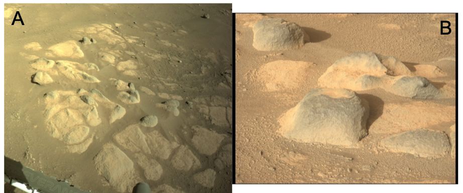
Figure 1: A. NavCam image of the workspace, sol 66 (N_LRGB_0066_RAS_0032208_CYP_S_STERONVJ01); B. MastCam image showing pavers and high standing dark-toned rocks (ZCAM03130). NASA/Caltech-JPL-MSSS/ASU.
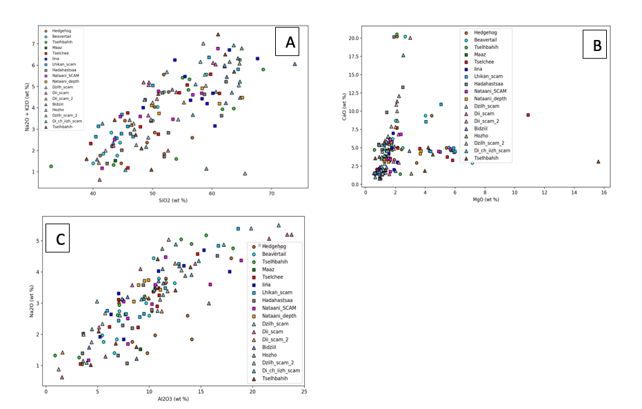
Figure 2: A. Na2O+K2O vs SiO2 content of the 19 rocks analyzed by SuperCam/LIBS. B. CaO vs MgO; C. Na2O vs Al2O3. Low standing rocks are shown as squares, High standing rocks as triangles, and float rocks as circles.
How to cite: Cousin, A., Anderson, R., Forni, O., Benzerara, K., Mangold, N., Beck, P., Dehouck, E., Ollila, A., Meslin, P.-Y., Gibbons, E., Gasnault, O., Beyssac, O., Lassue, J., Frydenvang, J., Vogt, D., Pilleri, P., Schröder, S., Clegg, S., Maurice, S., and Wiens, R.: Observations of Rocks in Jezero Landing Site: SuperCam/LIBS technique overview of results from the first six months of operations., Europlanet Science Congress 2021, online, 13–24 Sep 2021, EPSC2021-644, https://doi.org/10.5194/epsc2021-644, 2021.
Introduction: Meridiani Planum is a relatively plain area located at the Martian equator, south of Arabia Terra, approximately ranging from longitude 350°E to 10°E. Heavily cratered Noachian-aged terrains constitute the oldest geological unit in the region, where several channels and valley networks have left their imprint on the surface [1]. A series of younger terrains were then emplaced in some areas, likely during Late Noachian/Early Hesperian epochs [2].
Meridiani Planum shows signs of a diversified and complex history of aqueous activity in many locations. In addition to the evidence provided by the numerous valley networks, data from OMEGA and CRISM orbital spectrometers have revealed the presence of Fe/Mg phyllosilicates and sulfates throughout the area [3]. These hydrated minerals usually form by alteration in aqueous environments. Older, Noachian-aged, areas are generally characterized by the presence of Fe/Mg phyllosilicates, while younger capping units may display both phyllosilicates and sulfates. Regional differences in mineralogy, hydration, and morphology imply that the aqueous conditions probably varied over time.
Advancing our knowledge on the aqueous processes that left their imprint on this area could provide new insight on the past climate and habitability of Mars. Noachian terrains are of particular interest, as they date back to a period which is largely recognized as the most suitable for hosting habitable conditions on the planet.
Materials and method: We selected a small crater in the northern part of Meridiani Planum (figure 1), centred at 359.96°E, 2.45°N and approximately 20 km wide. The crater is part of the exposed Noachian-aged terrains of the region and is surrounded to the south and east by younger terrains, which overlie part of its ejecta.
Both mineralogical and geomorphological characteristics were investigated using MRO-based instruments CRISM, HiRISE and CTX. Infrared data (1.0-2.6 μm) from CRISM spectrometer was used to assess the mineralogical composition of the terrains inside the crater. This information was then integrated with HiRISE high-resolution camera data to identify and correlate with compositional information the different morphologies within the crater's area. Additionally, images from CTX camera were used to provide surrounding context.
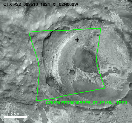
Figure 1: CTX image of the region of interest. The green lines trace CRISM footprint, showing the coverage of the spectral data analysed.
Results: Phyllosilicates, specifically Fe/Mg-rich smectite clays, are found in a wide area of the crater’s interior. The spectra obtained from CRISM are displayed in figure 2, they show absorption features near 1.4, 1.9, and 2.3 μm, with additional combination tones near 2.4 μm, and sometimes 2.5 μm. The exact position of some bands depends on the relative proportions of Fe and Mg: for example, the 2.3 μm band shifts to shorter wavelengths as Fe is exchanged for Mg [4].
We identify two distinct spectral classes for the smectites (Figure 2): the first is compatible with laboratory spectra of Fe-rich smectites, e.g. nontronite, while the second with the spectra of more Mg-rich smectites, such as saponite. The position and shape of the 2.3, 2.4 and 2.5 μm features are slightly different for the two classes. Figure 3 shows the absorption details for both CRISM and laboratory spectra.
Fe-rich smectites tend to be concentrated in limited areas of the crater, mostly close to its southern border. Further investigation is needed on this point to clarify the reasons for this specific distribution.

Figure 2: averaged spectra obtained for the areas which show the presence of Fe/Mg smectites: red is from predominantly Fe-rich smectite areas, green is from Mg-rich areas.
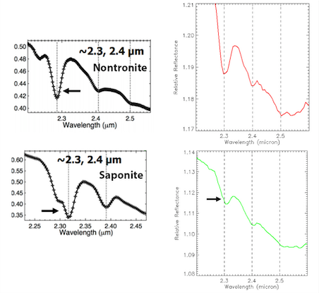
Figure 3: (left) Laboratory spectra of Nontronite (Fe-rich smectite) and Saponite (Mg-rich smectite). (right) Absorption details of the spectra from figure 2.
The spectral signature of the remaining terrains implies the presence of pyroxenes. Usually, these areas tend to be darker and dunes of a fine-grained material are frequently observed.
Terrains which retain signs of hydration show an interesting variety of morphologies, however, a common feature is that they all show polygonal fracture patterns to some extent (figure 4).
Figure 4: Cracking patterns on the crater’s hydrated terrains as observed with HiRISE. Approximate location is marked by a plus sign in figure 1.
Interpretation and discussion of the results: A possible explanation for the observed cracking patterns is related to desiccation. Desiccation is caused by water evaporation or migration: as a result of the water loss, the terrain shrinks and cracks.
Cracking patterns, correlating with the presence of sedimentary materials (e.g. clays or sulfates), are found in various Martian terrains and could be markers of ancient lacustrine environments [5]. The Noachian geologic setting, in association with terrains that show evidence of past aqueous activity, reinforces this hypothesis.
Noachian paleo-lakes are a top-priority setting for astrobiological research as they might have been suitable environments to support and preserve traces of microbial life [6]. Nevertheless, a different origin for these features is not ruled out and further investigation is required.
Conclusions: Meridiani Planum is undoubtedly an area which was subject to significant water alteration. Fe/Mg smectites detected in the northern Noachian-aged terrains of Meridiani Planum, in association with polygonal fracture patterns, could be related with the existence of ancient paleo-lake environments, making this area an interesting spot for astrobiological research. The information available on these areas is still limited: in order to provide context to MER Opportunity’s observations, previous studies mainly focused on the younger capping terrains lying south of the crater we examined. The results obtained here can be a worthwhile starting point for better understanding the evolutionary history of Meridiani Planum’s oldest terrains.
Acknowledgments: Featured camera images were obtained from NASA’s Planetary Data System (PDS).
References: [1] Williams et al. (2017) GRL, 44, 1669-1678. [2] Hynek et al. (2002) JGR, 107, 5088. [3] Flahaut et al. (2015) Icarus, 248, 269-288. [4] Viviano-Beck et al. (2014) JGR, 119, 1403-1431. [5] El-Maarry et al. (2014) Icarus, 241, 248-268. [6] Vago et al. (2017) Astrobiology, 17,471-510.
How to cite: Baschetti, B., Altieri, F., Carli, C., Frigeri, A., and Sgavetti, M.: Mineralogical and Geomorphological Characterisation of a 20-km-wide Crater in Older Meridiani Planum, Mars, Europlanet Science Congress 2021, online, 13–24 Sep 2021, EPSC2021-143, https://doi.org/10.5194/epsc2021-143, 2021.
Introduction
The recently landed Perseverance rover from the Mars2020 mission is the first rover to select samples with the future objective of taking them back to the Earth in the Mars Sample Return future mission. Until then, Martian meteorites are still the only samples that we have on Earth to study the composition and formation of Mars. Due to the scarce abundance and the importance of these samples, the development of non-destructive characterization methodologies is of great importance. In this case, the Martian Shergottite NWA1950, considered one of the less studied Martian meteorites, has been selected with the double objective of performing the characterization of its original and altered minerals and of contributing to ascertain the degradation reactions.
Experimental
Instead of using the classical methods of analysis, a non-destructive analytical methodology that make use of spectroscopic techniques has been used. This approach could also be employed to study other meteorites or even in the future returned samples from Mars. The analytical methodology proposed is mainly based on the effectiveness of Raman microscopy for the molecular characterization, assisted by Energy Dispersive X-Ray Fluorescence (ED-XRF) and Scanning Electron Microscopy with Energy Dispersive Spectroscopy (SEM-EDS) to clarify the distribution of elements in the sample. In addition, Raman microscopy and µ-ED-XRF imaging analyses also allows performing the characterization of the whole surface of the meteorite obtaining the molecular and elemental distributions maps respectively.
Results and Discussion
The applied methodology on the NWA1950 sample showed a main matrix composed of pyroxenes and olivines. The identification of pyroxenes showed the presence of both, ortopyroxenes (low in Ca) and clinopyroxenes (high in Ca). Different olivines with different proportions of fayalite (Fe2SiO4):forsterite (Mg2SiO4) were detected by Raman, specifically olivines varying from 63 to 77% of Mg content. The study of the olivines also showed different degradations on them. The most common degradation suffered by the olivines was the oxidation of part of the iron(II) resulting in the identification of hematite (Fe2O3) grains over olivines enriched in Mg content due to the partial Fe loss after its oxidation. In other cases, the oxidation of the iron present in the olivine lead to the formation of magnetite (Fe3O4). Both reactions should lead also to the formation of silica (SiO2) and this study has identified vitreous silica by Raman spectroscopy in the olivines with less than 69% Forsterire. This observation may indicate the initial oxidation of the olivine occurred on Mars and therefore the quartz was transformed into vitreous silica due to the high temperatures and pressures suffered by the meteorite after the shock.
Among the minor compounds, it is important to highlight the presence of ilmenite (FeTiO3). In this case, the Raman bands obtained for ilmenite are shifted to higher wavenumbers than the theoretical ones. This may be indicative of a shocked Ilmenite, subjected to the high pressures of the ejection, and therefore indicating its possible Martian origin. In addition, Ilmenite can be oxidized into TiO2 that can appear as different polymorphs, rutile and anatase mainly. In this case, the identified polymorph was anatase that is formed at low temperatures, indicating that anatase is not an alteration compound from Mars but rather a terrestrial alteration mineral formed after the oxidation of ilmenite once the meteorite was on Earth.
Merrillite (Ca9NaMg(PO4)7) was also detected as an important mineral phase in this meteorite. The elemental calcium and phosphorous ED-XRF distributions can be appreciated in Figure 1, showing the overlap between these two elements, matching perfectly with the molecular Raman distribution of merrillite in one of the faces of the meteorite.
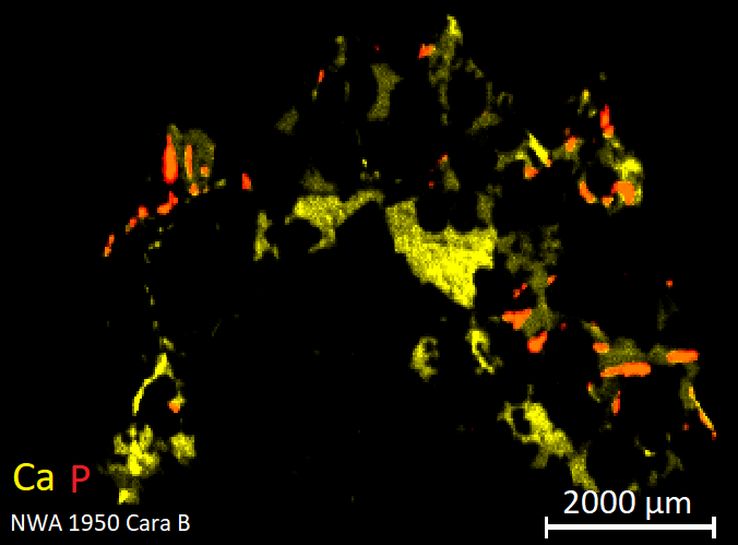
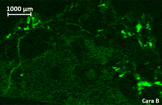
Figure 1. ED-XRF elemental distribution maps of Ca and P, showing in orange the overlaping of both elements (top) and the Raman image showing the molecular distribution of merrillite (down).
Iron chromites (FeCr2O4) were also detected, by means of Raman and SEM-EDS microscopic techniques, as abundant particles distributed all along the surface of the meteorite by means of Raman and SEM-EDS.
Two different calcites were identified by Raman microscopy. One of them is due to the presence of terrestrial calcite with its main characteristic band at 1086 cm-1. However, most were shocked calcites due to the shift of the main Raman band to higher wavenumbers (to 1088 and even to 1089 cm-1), suggesting again the effect of the pressure that suffered the meteorite and thus showing the Martian origin of these shocked calcites. The non-shocked calcites should be considered as terrestrial weathering compounds.
Finally, some sulfides were identified as chalcocite (Cu2S) and acanthite (β-Ag2S) by means of Raman and SEM-EDS microscopy. The origin of acanthite cannot be confirmed as Martian because if argentite (α-Ag2S), the high temperature stable phase of silver sulfide, was formed during the harsh conditions that suffered the meteorite during its ejection from Mars, the formation of argentite is reversible when the pressure ceases, and after the entrance in Earth atmosphere, the acanthite will be formed again.
Conclusions
As can be seen, the employed analytical methodology allowed us to characterize the original Martian mineral composition of the meteorite as well as the presence of alterations minerals originated in Mars but also after terrestrial weathering processes. In none of the analyses the sample was manipulated or treated chemically nor physically, all the measurements were performed over the surface of a thin section of the meteorite. Therefore, the same non-destructive analytical methodology could be followed for the characterization of other meteorites from other origins and also for the Mars samples when they are back on the Earth as first non-destructive characterization step that can lead to much information.
How to cite: Madariaga, J. M., Coloma, L., García-Florentino, C., Huidobro, J., Torre-Fdez, I., Aramendia, J., Castro, K., and Arana, G.: Characterization of original and altered mineral phases of the Martian shergottite NWA1950 by means of non-destructive analytical techniques. Implications for the analyses of future returned samples from Mars, Europlanet Science Congress 2021, online, 13–24 Sep 2021, EPSC2021-645, https://doi.org/10.5194/epsc2021-645, 2021.
There is a very significant body of evidence for a dense Martian atmosphere during the Noachian period, about 3.8 Ga ago. At that point in the evolution of the red planet water was present in the surface of Mars, and ancient surface features indicate that it flew through significant regions of its surface. We have studied Allan Hills 84001. an orthopiroxenite formed about 4.1 Ga ago. It is a meteorite widely known because [1] found microscopic structures that were suggested to be magnetotactic microbe fossils. In particular, in our CSIC laboratory I have studied with some of my PhD students the carbonate globules contained in this meteorite [2]. We discovered in a ALH84001,82 thin section (Fig. 1) that they were formed near the rock fractures, as consequence of the precipitation of Mg- and Fe-rich carbonates from an aqueous solution.
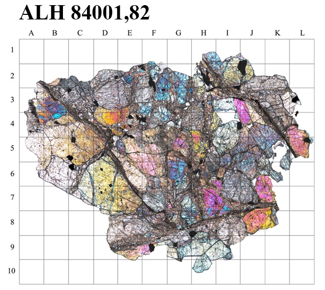
Figure 1. Thin section of ALH 84001. The square grid is mm-sized. This optical microscope transmitted light reveals the main minerals forming the rock and many fractures as consequence, at least, of two impacts while the rock formed part of Mars’ surface. Water penetrated into the fractures and produced the carbonate globules (see also Fig. 2)
Interestingly, we found distinctive layers in the walls of the carbonate globules. They indicate that the globules growth occurred under several flooding stages. As they exhibit differentiated elemental chemistry, it could reflect distinctive chemical solutes, being probably evidence of chemically-distinguishable fluids produced by environmental differences [3-4]. To explain liquid water presence at that time is challenging because the young Sun was less luminous than today: about was ~25% lower than nowadays. Consequently, being Mars about 1.5 times more distant from the Sun than the Earth, the solar energy available on Mars was ~1/3 of what gets the Earth today. Then we need to invoke an atmospheric greenhouse effect. Early Mars atmospheric composition is not well constrained, but it was probably mostly composed of CO2 with a surface pressure between a few hundreds of mbars to a few bars [5]. Large amounts of CO2 and H2O were probably released by the substantial Tharsis volcanism during the mid-Noachian. These species probably contributed, but other greenhouse gases have been proposed to solve the enigma (Fig. 3). Some of them are photochemically unstable and rapidly exhausted, unless continuously outgassed by volcanoes. The discovery of sulphate salts in Mars’ surface [5] have promoted the relevance of SO2 as greenhouse, and strength the possibility of an astrobiological catalytic environment in presence of water and N-bearing species [3-4]. The study at microscale of Martian meteorites (exemplified with the previous ALH84001 study) can be useful to understand the geological context and get new insight about the presence of biosignatures.
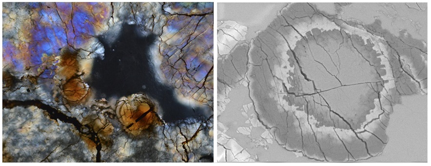
Figure 2. ALH 84001 carbonate globules. Left) Optical microscope transmitted light where the rounded globules appear in brown. Right) One of the globules emphasized with a EDX mapping to show the different Fe-content of the layering.
Concerning the presence of water in Mars’ surface and subsurface at different epochs, the evidence arrived from Martian meteorites indicates a progressive water depletion probably due to the evolving surface environment, finally reaching the current harsh conditions. For example, clear evidence for Amazonian acidic liquid water on Mars surface was found, producing aqueous alteration minerals [5]. A dense atmosphere associated with volcanic outgassing during the Noachian period could have promoted significant deceleration, and disruption of fragile chondritic asteroids. In such circumstances the arrival of meteorite powders was a way to promote catalytic reactions at the Martian surface. Given that the early Mars was subjected to a continuous rain of chondritic materials when it experienced significant hydrothermal activity, I identify a potential astrobiology environment
All this growing evidence about the role of the aqueous alteration and the formation of secondary minerals also supports the evidence for a wet Mars environment. The role of collisional gardening in the early stages of Mars' evolution is also out of doubt from the study of the oldest Martian meteorites [6]. In fact, new evidence for a massive water sequestration has been recently presented [7]. To search for the pathways of water towards the interior of Mars we should study impact fractures in the crust of Mars, and their role to host potential biota. Probably the transient nature of aquifers in Mars was restricting the regions to develop life, but future mission searches in depth could get new clues.
ACKNOWLEDGEMENTS
This research has been funded by PGC2018-097374-B-I00 (MCI-AEI-FEDER, UE). US Antarctic meteorites are recovered by the Antarctic Search for Meteorites (ANSMET) program funded by NSF and NASA, and characterized and curated by the Department of Mineral Sciences of the Smithsonian Institution and Astromaterials Acquisition and Curation Office at NASA Johnson Space Center.
REFERENCES
[1] McKay D. S. et al. (1996) Search for Past Life on Mars: Possible Relic Biogenic Activity in Martian Meteorite ALH 84001. Science 273, 924-930.
[2] Moyano-Cambero, C.E., Trigo-Rodríguez, J.M., Benito, M.I., et al. (2017) Petrographic and geochemical evidence for multiphase formation of carbonates in the Martian orthopyroxenite Allan Hills 84001, Meteoritics & Planetary Science 52, 1030-1047.
[3] Trigo-Rodriguez, J. M., Moyano-Cambero, C. E., Donoso, J. A., Benito-Moreno, M. I., Alonso-Azcárate, J. (2018) Clues on Past Climatic Environments and Subsurface Flow in Mars from Aqueous Alteration Minerals Found in Nakhla and Allan Hills 84001 Meteorites, 49th LPSC, LPI Contribution No. 2083, id.1448
[4] Trigo-Rodríguez, J. M., Moyano-Cambero, C. E., Benito-Moreno, M. I., Alonso-Azcárate, J. (2018) Growth of carbonate globules in ALH 84001 Martian orthopyroxenite by transient floods in a chemically variable environment. Proceedings of the Mars Science Workshop From Mars Express to ExoMars, held 27-28 February 2018 at ESAC, Madrid, Spain, id.71
[5] Fernández-Remolar D.C. et al., (2011) The environment of early Mars and the missing carbonates. Meteoritics & Planetary Science, Volume 46, 1447-1469.
[6] Humayun M. et al. (2013) Origin and age of the earliest Martian crust from meteorite NWA 7533. Nature 503, 513-516.
[7] Scheller, E. L., Ehlmann, B. L., Hu, Renyu, Adams, D. J., Yung, Y. L. (2021) Long-term drying of Mars by sequestration of ocean-scale volumes of water in the crust. Science 372, 56-62.
How to cite: Trigo-Rodríguez, J. M. and Trišić, J.: What can be learned from Allan Hills 84001 carbonate globules about aqueous alteration processes in the Martian crust?, Europlanet Science Congress 2021, online, 13–24 Sep 2021, EPSC2021-803, https://doi.org/10.5194/epsc2021-803, 2021.
1. Introduction
Olivine, (Mg, Fe)2SiO4, is a mineral composed of the two endmembers of its solid solution series: forsterite (Fo, Mg2SiO4) and fayalite (Fa, Fe2SiO4). It is a silicate mineral present in Mars usually alongside with plagioclase and pyroxene, as they are all present in basalts and igneous rocks. The forsterite and fayalite proportions in the olivine is a key factor in order to study this type of rocks.
Active and upcoming Mars missions will study areas of ancient Mars using, among others, Raman spectroscopy in the instrumental payload, being a relevant technique for space exploration. There are several papers proposing Raman spectroscopy to quantify the ratio Fo/Fa based on the wavenumbers of the two most intense bands. However, the proposed calibration models have an uncertainty of around 10 %, too high to obtain reliable conclusions form the studied samples. In this work a new model that greatly improves the accuracy and uncertainty is presented.
2. Data set
A collection of Raman spectra from olivines with a known composition was collected to develop a calibration model for the determination of the metallic content (Mg, Fe) of the mineral. The collection included 64 data points from 14 different research papers where different Raman instruments and acquisition parameters were used, which eliminates any possible bias that the instrumentation could introduce in the model. In addition to the set of olivines used for the calibration, a commercial pure olivine of known metallic concentration, Fo89.5±1.8Fa10.5±0.5, was used as the standard to validate the proposed models. This olivine was analyzed by WD-XRF and its mineral purity was checked by XRD. The Raman measurements were carried out with an Invia High Resolution micro-Raman spectrometer (Renishaw, UK) instrument, using a 532 nm excitation laser with a spectral resolution of 1 cm-1.
3. Results and Discussion
Two different regression curves were developed to characterize the olivine concentration ratio by Raman spectroscopy using their two main Raman features (OB1, 812-825 cm-1, and OB2, 837-857 cm-1). These regression curves with their residuals can be observed in Figure 1 and Figure 2 and their equations are shown in Equation 1 and 2, respectively. The two red lines depicted in the calibration curve plots represent the calculated confidence interval for all the data at a 95 % confidence level.
OB1 (cm-1) = 3.63·10-4·Fox2 + 0.0667·Fox + 814.2 (Equation 1)
OB2 (cm-1) = 3.00·10-4·Fox2 + 0.142·Fox + 839.6 (Equation 2)
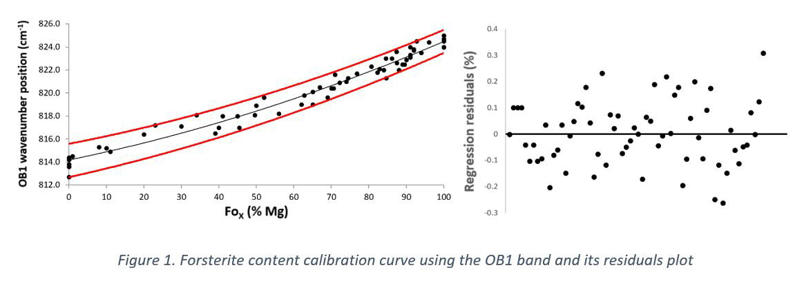
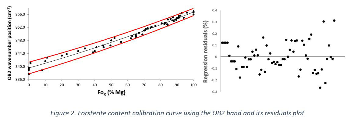
As can be observed, all the data used to develop both models fit inside the confidence interval, which implies that there are not outliers among the set of data used. Regarding its quality parameters, the determination coefficient (r2) obtained for the quadratic regression models expressed in Equation 1 and 2 are 0.970 and 0.984, with a typical error of ±0.61 and ±0.73, respectively. The uncertainties in both residual plots scattered randomly, without showing any trend. In addition, all the points are equally distributed around the zero horizontal line and all of them are at the same range of distance from it. All of these facts implies that the proposed models for the data set used are the correct ones and that the model’s predictions should be correct on average, rather than systematically too high or too low.
In order to check the accuracy of the two models, the standard commercial olivine described above was used (Fo89.5±1.8Fa10.5±0.5). The concentrations obtained using the OB1 and OB2 models can be observed in Table 1.
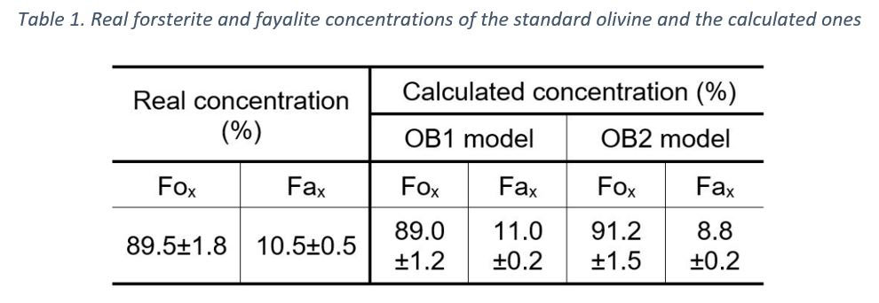
As observed, the OB1 and OB2 forsterite confidence interval results overlap perfectly with the real concentration confidence interval, which means that the predicted concentrations with these two models were correct. In addition to the standard olivine, the calibration models were tested using the 64 data values that were used for their development. The wavenumber position of OB1 and OB2 were introduced in the respective regression curves and the forsterite value corresponding to each value was calculated. On average, it was observed that the OB1 model had better accuracy for the forsterite rich olivines, while the OB2 model was better for the fayalite rich olivines. Thus, as a good compromise solution, the best alternative would be to always use both models and to average their result, independently on the forsterite and fayalite concentrations of the mineral. This method was tested with the standard olivine, obtaining an uncertainty of ±2.1 % for the forsterite content and of ±2.0 % for the fayalite one. Uncertainties given with the 95 % level of confidence using expanded uncertainty (k=2).
The proposed equations have been applied in the study of several Lunar and Martian meteorites where olivine is present. In the NWA 11273 Lunar meteorite olivine ranged from Fo56Fa44 to Fo83Fa17, a little bit broader than the values summarized in the Meteoritical Bulletin. In the NWA 10628 Martin shergottite, the Raman bands only showed the presence of fayalite, in agreement with the data from the Meteoritical Bulletin, while the Martian shergottites RBT 0462 gave a short range (Fo9.1±0.1Fa90.9±0.1), NWA 1950 a broader range (Fo60Fa40 to Fo80Fa20) and the DaG 735 the most extended range (Fo53Fa47 to Fo80Fa20).
4. Conclusions
The study of olivines by the active and upcoming Mars missions could provide very relevant information about the evolution of the geology of Mars. One of the key parameters of this mineral is its metallic content, in other words, the ratio of forsterite and fayalite that compose them. In this work, a method to calculate that ratio by averaging the results of two calibration models that use the two main Raman bands of the mineral is proposed. With this method, an uncertainty of only 2 % is achieved, which is a significant improvement over the models already developed in literature, which have an uncertainty of around 10 %. With this model, it should be possible to provide an accurate olivine metallic characterization for the olivine Raman spectra that are found on Mars.
How to cite: Torre-Fdez, I., Garcia-Florentino, C., Huidobro, J., Coloma, L., Ruiz-Galende, P., Aramendia, J., Castro, K., Arana, G., and Madariaga, J. M.: Characterization of olivines and their metallic composition: Raman spectroscopy could provide an accurate solution for the active and future Mars missions, Europlanet Science Congress 2021, online, 13–24 Sep 2021, EPSC2021-586, https://doi.org/10.5194/epsc2021-586, 2021.
Serpentinization and carbonation have affected ultramafic rocks on Noachian Mars in several places called here serpentinization-carbonation systems (SCS). Among the most prominent SCS revealing mineral assemblages characteristic of serpentinization/carbonation is the Nili Fossae region [1]. Jezero crater – the target of the Mars 2020 rover –hosted a paleolake which constitutes a sink for sediments from Nili Fossae [1]. Thanks to the near infrared spectrometer onboard Mars2020 [2], the mission has the potential to offer ground truth measurement for other putative serpentinization/carbonation system documented on Mars. Several important aspects that may be addressed are: Do carbonates result from primary alteration of olivine-rich lithologies or are they derived by reprocessing of previous alteration minerals [3]? What is the composition? and nature of the protolith, which appear to be constituted of considerable amounts of olivine [4]? To reveal critical information regarding the conditions of serpentinization/carbonation, accessory minerals need detailed studies [1; 5]. In case of Jezero Crater, and serpentinization on Mars in general, the main alteration minerals are identified, but little is known about the accessory minerals.
The Nili Fossae-Jezero system has potential analogues in terrestrial serpentinized and carbonated rocks, such as the Leka Ophiolite Complex, Norway (PTAL collection, https://www.ptal.eu). Here, distinct mineral assemblages record different stages of hydration and carbonation of ultramafic rocks [6].
We perform petrological and mineralogical analyses on thin sections to characterize the major and trace minerals and combine with Near Infrared (NIR) spectroscopy measurements. A set of spectral parameters are defined and compare to spectral parameters previously used on CRISM and OMEGA data [1, 4, 7, 8]. We study the significance of the mineralogical assemblages including nature of accessory minerals. Effect of the presence of accessory minerals on the NIR signal is investigated and their potential incidence on the amount of H2/CH4 production in mafic or ultramafic system is discussed [5].
We started to apply the newly defined spectral parameters on several SCS on Mars. Results confirm local carbonation of earlier serpentinized rocks and suggest that different protoliths could have led to diversity of mineralogical associations in SCS on Mars. Multiple detection of brucite are also suggested for the first time on Mars. Altogether our results help to better describe key geochemical conditions of the SCS on Mars for habitability potential of the martian crust and Mars’s evolution.
References:
- Brown, A. J., et al. EPSL1-2 (2010): 174-182.
- Wiens, R.C., et al. Space Sci Rev217, 4 (2021).
- Horgan, B., et al. Second International Mars Sample Return. Vol. 2071. 2018.
- Ody, A., et al. JGR: Planets2 (2013): 234-262.
- Klein, F., et al. Lithos178 (2013): 55-69.
- Bjerga, A., et al. Lithos227 (2015): 21-36.
- Viviano-Beck et al, JGR: Planets 118.9 (2013)
- Viviano-Beck et al, JGR: Planets 119.6 (2014)
How to cite: bultel, B., Krzesinska, A. M., Loizeau, D., Poulet, F., Astrheim, H. O., Bjerga, A., Harrington, E. M., Viennet, J.-C., Dypvik, H., and Werner, S. C.: Leka Ophiolite Complex as analogy to the serpentinization-carbonation system on Mars., Europlanet Science Congress 2021, online, 13–24 Sep 2021, EPSC2021-230, https://doi.org/10.5194/epsc2021-230, 2021.
The mineralogy of paleolake sediment strata at the high elevation (~4300 m) Lejía depression in the Altiplano region of Chile reflect evolution of the lake geochemistry over time. This mineralogical study is part of a larger project characterizing the geochemistry and biology of several samples from a paleo terrace of the Lejía lake region. Visible/near-infrared (VNIR) reflectance measurements of several samples reveal variations in gypsum, carbonate, clays, iron oxides/hydroxides, and halite with depth. The spectral features are also consistent with abundant allophane or related poorly crystalline clay phases. Mg-calcite, gypsum, and poorly crystalline clays dominate the surface materials, while each of these components varies with depth at our study site. Sediments at Gale crater on Mars also include abundant poorly crystalline phases, phyllosilicates, gypsum, halite, and iron oxides/hydroxides. Thus, characterizing the spectral properties of paleolake sediments from the Lejía region may help constrain the spectral signatures of Gale crater sediments and other sites measured from orbit.
Study Site. The broader Altiplano region of Chile provides an analog for Mars due to its extremely dry and salty conditions and this study was carried out as part of the SETI Institute team’s NASA Astrobiology Institute project (Cabrol et al., 2017). The Lejía region differs from others in the Chlean Altiplano due to its higher pH environment and the presence of clay minerals and carbonates in addition to the ubiquitous gypsum and halite otherwise characteristic of the Atacama region. Laguna Lejía is a shallow, salty lake spanning ~1 km in a depression between Láscar and other volcanoes in northern Chile where a larger glacial lake (10-15 km across) once stood (Grosjean et al., 1995). This high altitude basin is battered by winds and receives only limited precipitation, mostly from melting snow and ice from the surrounding mountains. Despite limited water, high UV radiation, and cold temperatures, zooplankton communities are present at Laguna Lejía (Muñoz-Pedreros et al., 2013). Further, genome-resolved metagenomics investigations are currently being developed to characterize the communities of microorganisms and their metabolisms in the paleo sediments of the Lejía lake (Lezcano et al., in preparation).
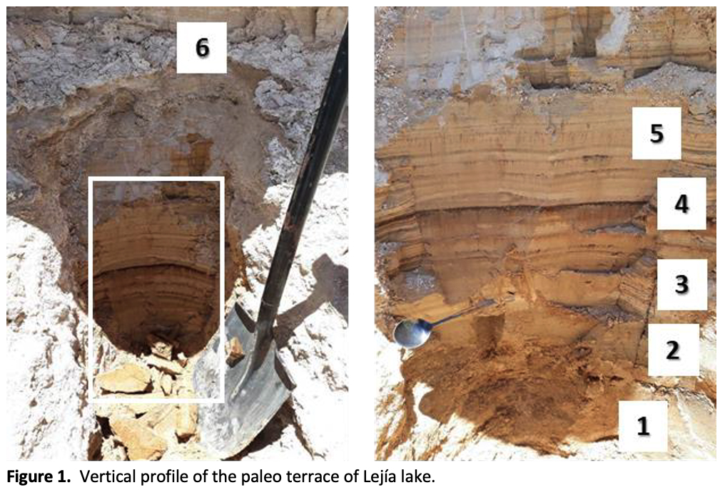
Samples. The paleolake sediments investigated here were collected in 2018 from the upper 1 m of a lake terrace (Figure 1) adjacent to the current Lejía lake. The samples were kept frozen until studied. Extensive analyses are underway including X-ray diffraction (XRD), major element analyses, δ13C and δ15N isotope analyses, metagenomics, and lipid analyses (Lezcano et al., in preparation). XRD analyses determined the presence of albite, anorthite, Mg-calcite, gypsum, halite, andesine, muscovite, and quartz in many of these samples. Aliquots of 6 samples collected from different horizons were thawed, then air dried in the lab, gently crushed and dry sieved to <125 µm, 125-250 µm, and 250-1000 µm size fractions. For this study, we are focusing on the mineralogy and spectral properties of these samples in order to ground truth observations of similar materials on Mars via the CRISM VNIR spectrometer (Murchie et al., 2009).
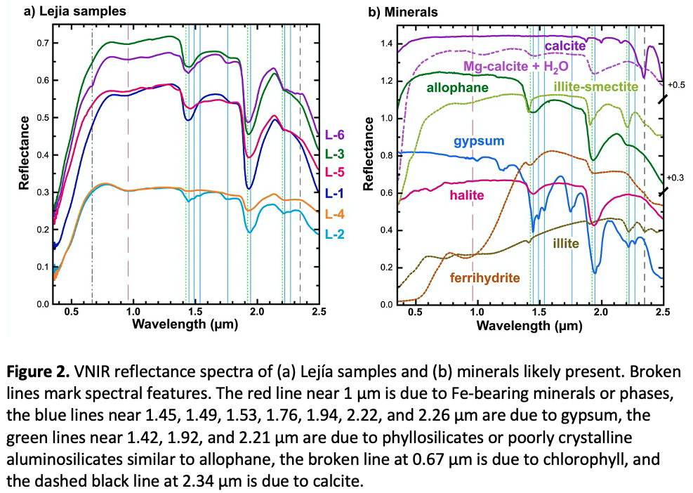
Spectroscopic Analyses. Reflectance spectra of bulk sample materials and size fractions from each strata were measured using a FieldSpecPro ASD spectrometer from 0.35-2.5 µm relative to Spectralon. Spectra in this range include bands and features due to phyllosilicates, sulfates, carbonates, hydrous phases, and Fe-bearing minerals (e.g., Bishop, 2019).
Results. VNIR spectra of the Lejía samples (Figure 2) exhibit changes with depth (Figure 1). Samples L-1, L-3, L-5, and L-6 are brighter overall and have stronger bands near 1.4 and 1.9 µm due to bound or adsorbed H2O in the samples (Figure 2a). These broad bands are most consistent with poorly crystalline aluminosilicates similar to allophane or to halite (NaCl) (Figure 2b). Mg-calcite is also present in some samples and would contribute a band near 2.34 µm. Some samples also contain feldspar and quartz, which would increase the spectral brightness but do not have spectral features in this range. Samples L-2 and L-4 have darker spectra, stronger bands near 0.97 µm due to Fe-bearing phases, and weaker water bands. Sample L-2 has the strongest bands due to gypsum, which is consistent with the XRD results. Sample L-6 also has some features due to gypsum. Compositional changes with depth highlight episodic variations in inputs to the lake over time.
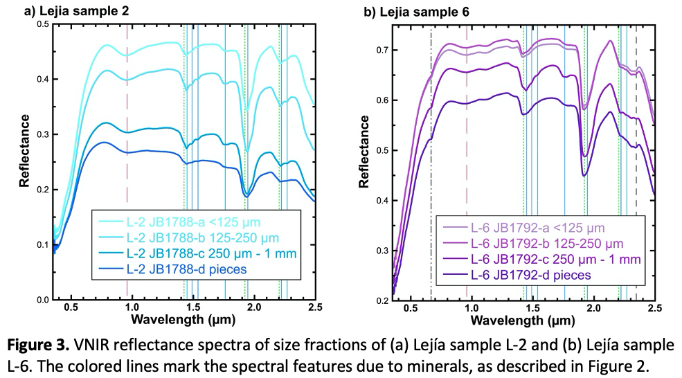
VNIR spectra for multiple size fractions of samples L-2 and L-6 document increases in spectral brightness typical for smaller particles as expected (Figure 3). Other small changes in the spectral properties are due to compositional variations associated with particle size. The VNIR spectra of L-2 are dominated by gypsum features at 1.45, 1.49, 1.53, 1.76, 1.94, 2.22, and 2.26 µm, but the coarse-grained samples include shifts in the bands near 1.4 and 1.9 µm towards shorter wavelengths, which is more consistent with phyllosilicates or allophane. The VNIR spectra of L-6 exhibit more variations with particle size due to the heterogeneous nature of this sample.
This VNIR spectroscopy study of paleolake samples from Lejía demonstrates detection of alteration minerals in these sediments that can be used for interpretation of the martian orbital spectra at Gale crater and related sites on Mars and subsequently for constraining the aqueous geochemical environment on Mars.
References:
Bishop, J. L. (2019) Visible and near-infrared reflectance spectroscopy of geologic materials. In: Remote Compositional Analysis: Techniques for Understanding Spectroscopy, Mineralogy, and Geochemistry of Planetary Surfaces. Cambridge University Press. 68-101.
Cabrol, N. A. and the SETI NAI Team (2017) From habitability to habitat – The current knowledge leaps and gaps in the search for biosignatures on Mars. AbSciCon, Mesa, Arizona. Abstract #3033.
Grosjean, M., Geyh, M. A., Messerli, B. & Schotterer, U. (1995) Late-glacial and early Holocene lake sediments, ground-water formation and climate in the Atacama Altiplano 22–24°S. J.Paleolimnology, 14, 241-252.
Muñoz-Pedreros, A., De los Ríos, P. & Möller, P. (2013) Zooplankton in Laguna Lejía, a high-altitude Andean shallow lake of the Puna in northern Chile. Crustaceana, 86, 1634-1643.
Murchie, S. L., et al. (2009) The Compact Reconnaissance Imaging Spectrometer for Mars investigation and data set from the Mars Reconnaissance Orbiter's primary science phase. JGR, 114, E00D07.
How to cite: Bishop, J. L., Lezcano Vega, M. Á., Parro, V., Cabrol, N. A., Sánchez-García, L., Warren Rhodes, K., and Hinman, N. W.: VNIR Spectral Analyses of Paleolake sediments at Lejía in the Altiplano region of Chile, Europlanet Science Congress 2021, online, 13–24 Sep 2021, EPSC2021-453, https://doi.org/10.5194/epsc2021-453, 2021.
Abstract
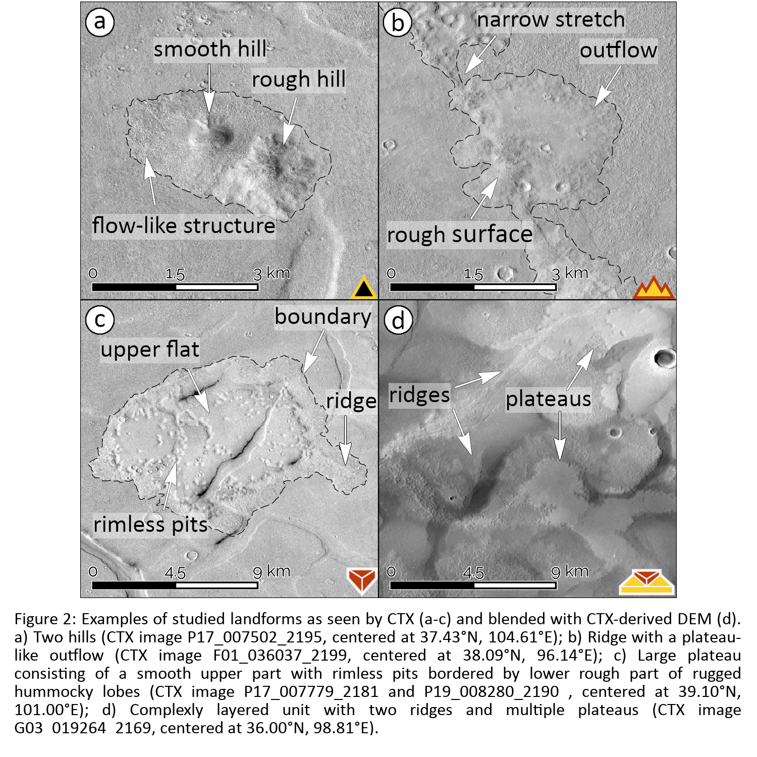
Here we present the results of our mapping of a large field of landforms characterized by flow-like morphology in the southwestern part of Utopia Planitia. They have been previously interpreted as mud flows associated with a partly frozen muddy ocean [1,2]. We find that these features can be grouped into four separate classes with distinct shapes and sizes and a clear evolutionary sequence among them. This suggests that all 205 studied features spread across the 500 × 1300 km large area were formed by the same basic process and that the material likely originated from the same source.
Introduction
The deepest parts of Utopia Planitia served as depocenters or sinks since early in the Martian history [2,3] and would be the final destination for any material released during Hesperian catastrophic floods [4]. Consequently, it was proposed that a large body of water might once or repetitively have been present there [1,5]. However, such hypothesis is still controversial due to the lack of unambiguous morphological evidence [6]. A promising area to search for such evidence is Adamas Labyrinthus, where the presence of putative mud flows has been previously reported [2,5].
Data and Methods
Our mapping is based on the global CTX Mosaic (5m/pixel) [7] which served as the base map for delineation of the observed features. The features were marked as point, linear, and polygonal features in a QGIS environment. HiRISE (0.3 m/pixel) and CTX stereo pairs were processed using the MarsSI service [8] to produce digital elevation models (DEM) for some studied landforms. This enabled us to calculate their basic morphometric characteristics, height and volume, but also to reveal the relative stratigraphy among them and their surroundings.
Results
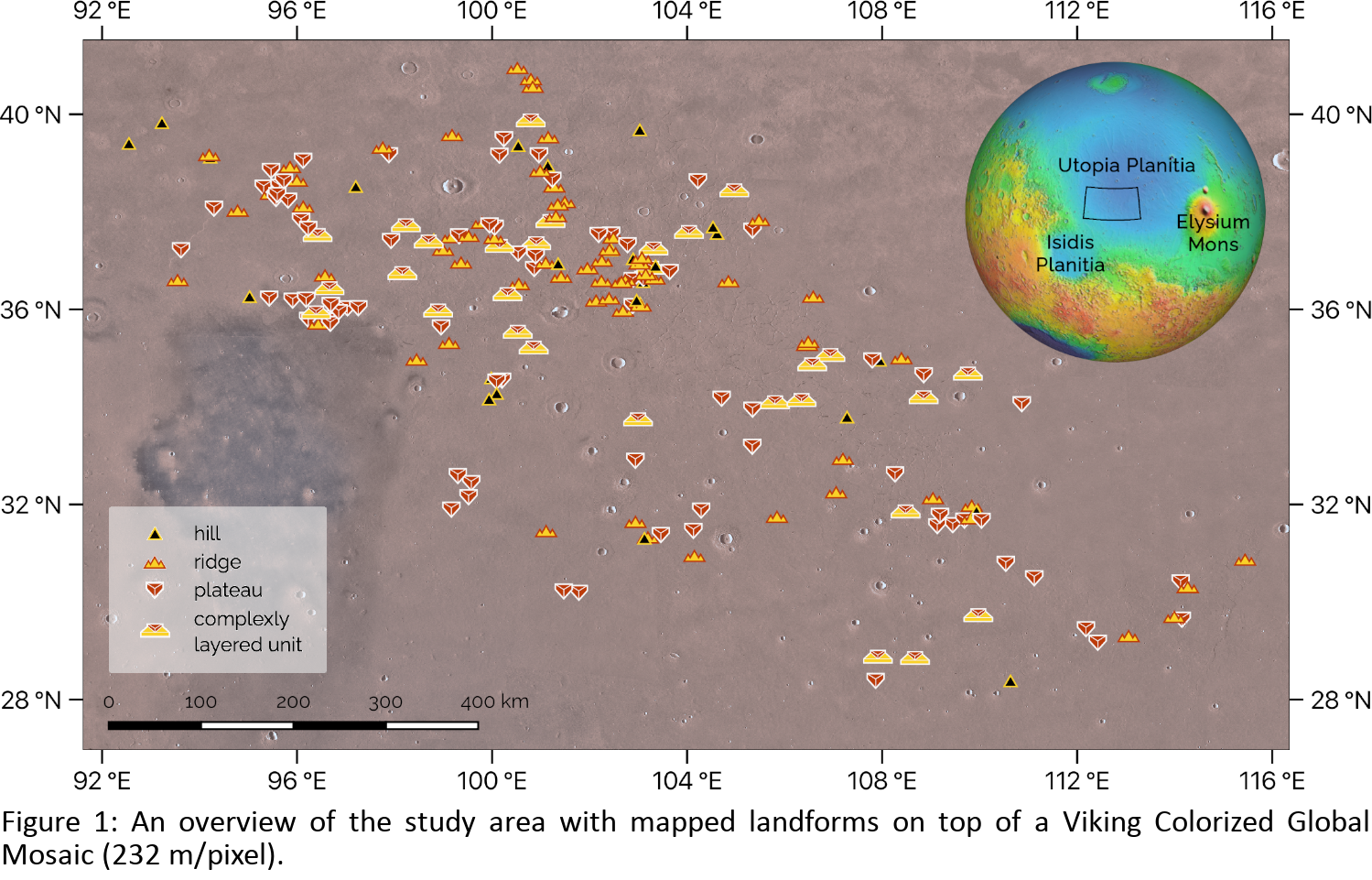
We found and mapped 205 features with positive topography characterized by flow-like appearance (Fig. 1). We classified them into four groups based on their extent, shape, and morphological properties (e.g., surface roughness). The resulting classes are ‘hills’ (Fig. 2a), ‘ridges’ (Fig. 2b), ‘plateaus’ (Fig. 2c), and ‘complexly layered units’ (CLUs, Fig. 2d), but we note that landforms commonly show transitional stages, hence share characteristics of multiple classes (such as in Fig. 2b).
Hills are the smallest studied features. They are characterized by circular plan-map appearance. Their surface texture can be either smooth or rough with flow-like structures extending beyond their bases (Fig. 2a). Hills can be solitary features or be associated with fractures, in which case they form hill chains. Ridges are elongated features with rough surface. They vary in width from narrow sub-kilometer stretches to wide and elevated smooth plateau-like features (see Fig. 2b) surrounded by hummocky rims. Plateaus (referred to in [2] as “etched flows”) are kilometer-sized features characterized by a smooth central uplifted unit usually surrounded by a rough boundary (Fig. 2c). The smooth unit often contains rimless pits. Plateaus sometimes superpose the polygonal throughs typical for Adamas Labyrinthus. The final type are CLUs represented by extensive and often chaotic combination of overlapping landforms mentioned above (Fig. 2d). Their relative stratigraphy is decipherable only with the use of DEMs.
Discussion
Previously, many flow-like features have been described elsewhere on Mars as lava flows [9,10]. At the first glance this might seem like a plausible scenario even here as the studied features bear many morphological similarities with terrestrial and martian lava flows. However, our survey did not reveal signs of subsidence or explosive excavation associated with studied features, which are commonly accompanying volcanic eruptions [e.g. 9,10]. We also did not find evidence of lava-water interactions (e.g., rootless cones) which would have favorable conditions to occur at this location as the studied features are superposed on terrain enriched in volatiles as documented by polygonal troughs, ghost craters and pedestal craters [2].
Instead, the morphological characteristics of the mapped features, transitions between their categories and the spatial context of the study suggest that the landforms are of sedimentary (mud) volcanic origin. Recently, Brož et al. [11] showed experimentally that low viscosity mud effusively emplaced onto the cold martian surface under the low atmospheric pressure of 7 mbar would behave similar to pahoehoe lava, and resulting landforms might have similar appearance. This is because the evaporative cooling of water would cause the formation of an icy crust on the surface of the mud flow, analogous to a solidified lava crust. This process might explain the observed shapes of the studied features.
Conclusions
We propose that the studied features were formed due to the expulsion of mud from a gradually freezing muddy body. Because of the climatic conditions on Mars such body would be freezing from the top down, causing an increase in the internal pressure of the still liquid mixture underneath. This would trigger the ascent of the mud towards the surface via cracks in the frozen crust and subsequent effusive eruptions. Once the mud would be exposed to the surface, it would spread by flowing over the surface, while freezing at the same time. This would limit its ability to flow but cause the resulting outflow to have an appearance similar to terrestrial lava flows. This process gave rise to the observed hills, ridges, plateaus and complexly layered units. Emergent landforms degraded over time as the volatile part of the compound sublimed away eventually leading to the characteristic morphology we observe today.
Acknowledgements:
VC, PB & YM were supported by Czech Science Foundation (#20-27624Y).
References:
[1] Jöns (1985), Lunar Planet. Sci. 16, 414–415; [2] Ivanov et al. (2014), Icarus 228, 121-140; [3] Frey et al. (2002), Geophysical Research Letters 29, no. 10, 22-1-22-4; [4] Carr (1996), Planetary and Space Science 44, 1411-1423; [5] Ivanov et al. (2015), Icarus 248, 383-391; [6] Sholes et al. (2021), Journal of Geophysical Research: Planets 126, no. 5; [7] Dickson et al. (2018), 49th Lunar and Planetary Science Conference 2018, LPI Contrib. No. 2083 ; [8] Quantin-Nataf et al. (2018), Planetary and Space Science 150, 157-170; [9] Hodges & Moore (1994), Atlas of volcanic features on Mars; [10] Hauber et al. (2009), JVGR 185, 69-95; [11] Brož et al. (2020), Nat. Geo. 13, 403-407
How to cite: Cuřín, V., Brož, P., Hauber, E., and Markonis, Y.: Mud flows in the Southwestern Utopia Planitia, Mars, Europlanet Science Congress 2021, online, 13–24 Sep 2021, EPSC2021-382, https://doi.org/10.5194/epsc2021-382, 2021.
Introduction: High-resolution images show the presence of kilometer-sized flows (KSFs) on Mars. Most of KSFs are associated with well-known volcanic centers, hence they have been interpreted as lava flows [1,2]. However, some KSFs occur in regions where such link is not obvious and processes related to sedimentary volcanism have been proposed as an alternative [3-7]. A remarkable example of such KSF was reported by Komatsu et al. [6,8] at the southern margin of Chryse Planitia (19.16°N; 322.71°E). Later thirty-five similar KSFs (e.g., Fig. 1a) have been observed in the region [7]. KSFs typically feature three morphological elements: a) a central depression from which channel(s) originate(s), b) leveed channel(s), c) a distal portion of the fading channel where the material is deposited forming terminal lobes.
Brož et al. [7] proposed that the KSFs resulted from low viscosity mud extrusions that propagate through extensive networks of channels that gradually lose their transport energy. As initial studies were based on Context Camera (CTX) images (~5-6 m/px, [9]) and HiRISE images (~30 cm/px; [10]), they lacked topographic resolution to support these hypotheses. Currently, six KSFs are covered by HiRISE stereo pairs. Using established methods [11], we generated seven Digital Elevation Models (DEMs) with a ground sampling of 1-2 m/px to obtain additional insights about their origin.
Observations: Studied KSFs show a topographically well-defined “source” area displaying circular, semicircular or elongated map-view outline (Figs. 1, 2a). Three source areas are situated on relatively flat plains and are surrounded by ~hundred(s) of meter-wide elevated rims (Fig. 2a). The other source areas are superposed on higher elevation/inclined pre-existing surfaces with laterally less extensive rims (Fig. 1). The elevation difference between source area floors and the rims ranges from 10 to 20 m. The elevation of the source area floors is the same as that of the flat plains beyond the elevated margins on which KSFs are superposed. The margins of all studied source areas are breached, enabling any extruded fluid to flow out. The presence of elevated mounds (<10 m high), or linear ridges (e.g. Fig. 1b) was observed inside the three source areas superposed on the inclined surfaces. There are two distinct types of margin. One type is characterized by scarps several meters-high (Fig. 2a), whereas the other type has a smooth topographic transition into the surroundings, yet a distinct albedo contrast in visible data (on Fig. 2b marked as bright units).
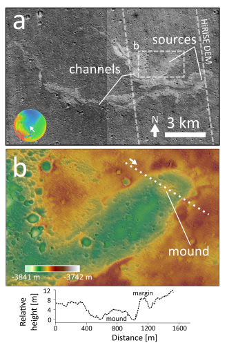
Figure 1: a) Example of studied KSF with position of HiRISE DEM marked. Base map: CTX mosaic (20.22°N and 324.06°E). b) Topography of the source area with position of the central mound and cross-profile marked (HiRISE DEM). North is up. Bottom: topographic cross profile across the source area in b.
Discussion: Our observations support the previous notions [6,7] that KSFs are aggradational, not degradational features. The inclination of the surface as well as the shape of source areas are in agreement with the suggestion that liquid material has been released from the source directly onto the pre-existing surface [7]. No signs of subsidence or explosive excavation were observed, which might be expected if these features were formed by volcanism [e.g., 12]. The mounds inside the source areas are not morphologically consistent with collapse of the rim of the source area, but could be the site where extruded material emerged at the surface and hence could mark the position of feeding conduits.
Our observations also reveal that the margins surrounding the channels are not continuous. Instead they are cut by channels joining the main channel to the bright units (Fig. 2b). No significant deposits were observed in these areas of distinct brightness, which would be expected in case of igneous eruptions (even in the case of very low viscosity lavas). This suggests that the liquid medium was capable of a dual behavior; forming elevated margins and propagating into the surroundings without displaying defined topographical boundaries at the surface.
We therefore propose a scenario that involves the release of water-rich sediments capable of both depositing onto the surface, and then spreading laterally over a wide area. During transport, levees formed on the margins of the channels. However, when the water-saturated sediments became unconfined, they spread laterally and thinned. The mixture then froze and later the ice sublimated away without leaving a detectable topographic expression, but instead changing the brightness of the surface.
Conclusions: Our study reveals that the morphology of KSFs in Chryse Planitia is consistent with the movement of low-viscosity mud across the surface during which the deposition of sediment caused the formation of leveed flow margins. The subsequent sublimation of ice removed substantial volume from the terminal parts of the flows. This supports the hypothesis proposed by [6,7] that these features are martian mud flows, formed by subsurface sediment mobilization. These features represent a window into the subsurface and an interesting target for in-situ investigation [14].
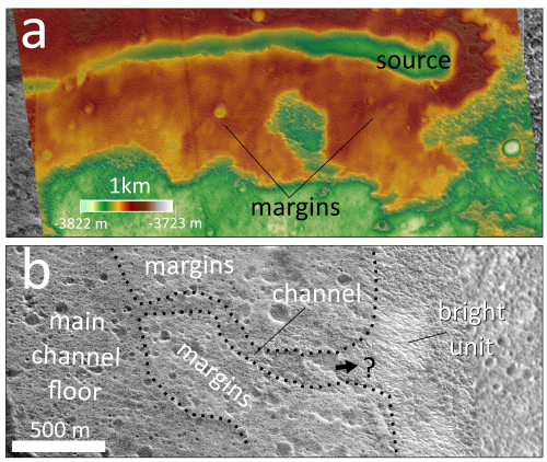
Fig. 2: Details of margins of two different KSFs in the area of interest. a) A source area superposed on relatively flat plain surrounded by km-wide margins, 19.36°N, 323.96°E (HiRISE DEM). b) Channel transitioning into a bright unit towards East (HiRISE image, 19.11°N, 322.735°E). North is up.
Acknowledgments: PB & YM were supported by Czech Science Foundation (#20-27624Y). SJC & AN are supported by the French Space Agency CNES for their HiRISE related work. AM is supported by the Research Council of Norway (#223272-288299).
References: [1] Hodges & Moore, 1994. Atlas of volcanic features on Mars. [2] Hauber et al., 2009. JVGR 185, 69-95. [3] Skinner & Tanaka, 2007. Icarus 186, 41-59. [4] Wilson & Mouginis-Mark, 2014. Icarus 233, 268-280. [5] Okubo, 2016. Icarus 269, 23-37. [6] Komatsu et al., 2016. Icarus 268, 56-75. [7] Brož et al., 2019. JGR-P 124,703-720. [8] Komatsu et al., 2011. Planet. Space Sci. 59, 169-181. [9] Malin et al., 2007. JGR 112, E05S04. [10] McEwen et al., 2007. JGR 112, E05S02. [11] Moratto et al., 2010. LPSC 41 #2364. [12] Brož & Hauber, 2013. JGR-P. 118, 1656-1675. [13] Brož et al., 2020. Nat. Geo. 13, 403-407. [14] Komatsu & Brož, LPSC2021 #1164.
How to cite: Brož, P., Hauber, E., Conway, S. J., Luzzi, E., Mazzini, A., Noblet, A., Jaroš, J., and Markonis, Y.: The Formation of the Kilometer-sized Flows in Chryse Planitia (Mars), Europlanet Science Congress 2021, online, 13–24 Sep 2021, EPSC2021-77, https://doi.org/10.5194/epsc2021-77, 2021.
Introduction
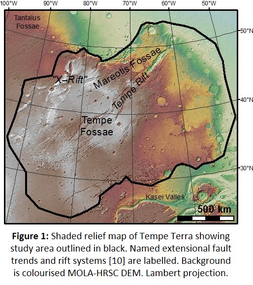
The structurally complex region of Tempe Terra, at the north-eastern edge of the Tharsis Rise, is of substantial interest for understanding the tectonic history of Tharsis, and Mars more broadly. Tempe Terra is a plateau consisting largely of Noachian to Hesperian volcanic and highland units [1], and it preserves evidence of tectonic activity across the lifespan of the Tharsis complex, from faulting of ancient Noachian crust to volcanic and tectonic activity through the Amazonian [2]. Fundamental work on the structural evolution of Tempe Terra [e.g. 2–5] was done with Viking Orbiter imagery and the 1986 geological map of Scott and Tanaka [6]. But in light of revised geological unit ages [1] and the higher-resolution image data now available, that structural evolution requires revisiting.
We present an updated inventory of structures in the Tempe Terra region, based on interpretation of recent, high resolution data. We utilised a detailed mapping approach at a regional scale to capture the area’s full tectonic complexity. Our work includes qualitative analysis of the regional structural trends, revised groupings and chronologies of constituent tectonic structures, and statistical characterisation of the fault populations present. First analysis shows that the total population of fault lengths is best described by a lognormal distribution, potentially indicating the impact of geological layering on development of the system. This work will lead to a revised structural history and assessment of stress regime evolution for Tempe Terra.
Methods
We undertook photogeological mapping at a scale of 1:300,000 across a study area 2.3 million km2 in extent (Fig. 1), primarily using High Resolution Stereo Camera (HRSC) images (of resolution 12–25 m/pixel, Mars Express). Thermal Emission Imaging System (THEMIS) image mosaics (at 100 m/pixel, Mars Odyssey) were used to aid mapping interpretation in areas of poor HRSC data quality. The focus of the mapping was normal faults, although other features including pit crater chains, wrinkle ridges, and chasms were also identified (but are not further discussed here). We mapped faults in a direction consistent with the right-hand rule for fault dip (i.e. 45° strike for a SE-dipping fault, 225° strike for a NW-dipping fault). Faults were grouped into sets, taking into consideration their orientation, morphology, crosscutting relations, absolute model age from associated geological units, and genetic relations (e.g. circumferential faults around volcanic centres). Erosional processes have affected existing structures at the plateau edges to the north and south, making some landforms ambiguous and their interpretation challenging.
Each mapped fault was assigned values for strike, length, and inferred dip direction (taken as 90° to the right of the fault strike), to help quantitatively characterise each fault set. We also assessed fault scaling properties by comparing functions for the cumulative frequency distribution of fault lengths with the Maximum Likelihood Estimators (MLE) function of the FracPaQ toolkit in MATLAB [7, 8]. Such analyses can help establish the mechanical properties of faulted rock, with power-law (fractal) distributions of fault lengths commonly described for deeply penetrating structures, and exponential distributions for faults in a brittle layer of restricted thickness [9].
Results
We mapped ~27,000 faults across the study area, allowing for detailed characterisation of the structural complexity of Tempe Terra. The dominant regional fault orientations are NE to ENE (Fig. 2), broadly similar to the long-recognised Tempe Fossae and Mareotis Fossae fault systems (Fig. 1), respectively [6]. We classified the total fault population we mapped into 20 separate fault sets, some of which are regionally extensive whereas others are locally confined. The bulk of extensional structures are concentrated through the centre of the region in a wide NE-trending zone; with few faults visible to the south-west, where crustal shortening structures (dominantly wrinkle ridges) are the principal feature, and to the north-west, likely because of burial by more recent lava flows.

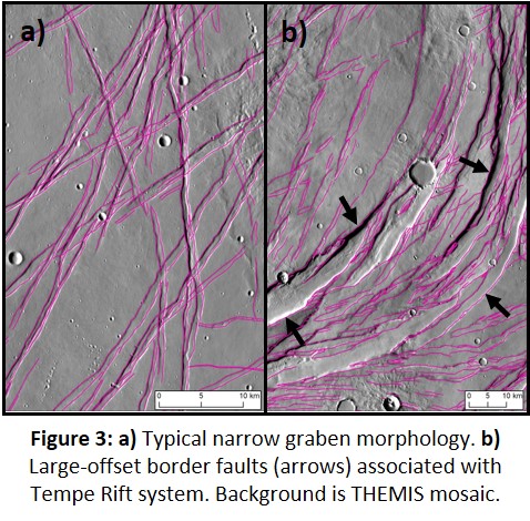
Normal faults across Tempe Terra occur as clearly defined graben (Fig. 3a), which are typically long and narrow (1–2 km wide on average), with segmented bounding faults. The exception to this trend is extensional faulting associated with the Tempe Rift and ‘X-Rift’ systems (Fig. 1, [10]), which in places form wider and deeper rift graben with multiple larger-offset (up to 3 km throw) border faults linked by relay ramps (Fig. 3b). This dominance of full-graben geometry across the region is also reflected by the bimodal distribution of fault orientations.
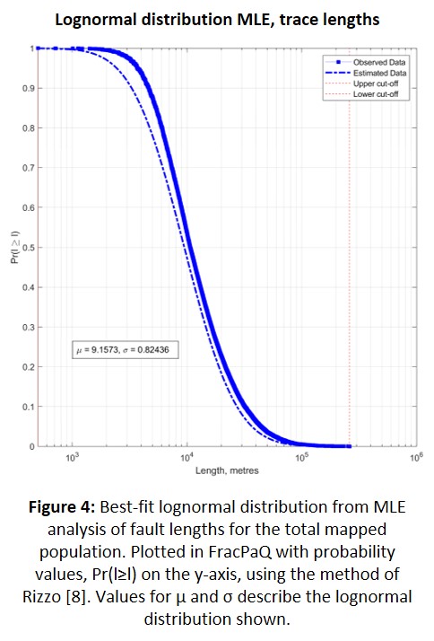
Mapped fault lengths range from 800 m to 202 km, although only 34% of the faults are ≥10 km long. MLE analysis of all fault lengths indicates the total population is not well described by an exponential distribution, nor by a power-law distribution without significant truncation of the small size fraction of the data. The best fit is a lognormal distribution (Fig. 4), which indicates either a truncated power-law population with underrepresentation of very small faults due to mapping resolution bias, or a true representation of the system with the observed length scale resulting from geological layering [9, 11].
Summary
Detailed fault mapping has allowed us to begin to characterise the full complexity of structures at, and geological evolution of, Tempe Terra. Ongoing analysis will lead to a new, comprehensive understanding of the history of this region, including an assessment of how regional and local stress regimes have evolved and interacted through time.
References
[1] Tanaka K.L. et al. (2014) USGS Scientific Investigtions Map 3292.
[2] Scott D.H and Dohm J.M. (1990) LPSC XX pp. 503-513.
[3] Fernández C. and Anguita F. (2007) JGR: Planets Vol 112(E9).
[4] Golombek M. et al. (1996) JGR: Planets Vol 101(E11) pp. 26119-26130.
[5] Hauber E. and Kronberg P. (2001) JGR: Planets Vol 106(E9) pp. 20.587-20602.
[6] Scott D.H. and Tanaka K.L. (1986) USGS I-Map 1802-A.
[7] Healy D. et al. (2017) JSG Vol 95 pp. 1-16.
[8] Rizzo R.E. et. Al. (2017) JSG Vol 95 pp. 17-31.
[9] Schultz R.A. et al. (2010) JSG Vol 32(6) pp. 855-875.
[10] Hauber E. et al. (2010) EPSL Vol 294 pp. 393-410.
[11] Bonnet E. et al. (2001) Reviews of Geophysics Vol 39(3) pp. 347-383.
How to cite: Orlov, C., Bramham, E., Thomas, M., Byrne, P. K., Mortimer, E., and Piazolo, S.: Detailed structural mapping of the Tempe Terra region, Mars, Europlanet Science Congress 2021, online, 13–24 Sep 2021, EPSC2021-315, https://doi.org/10.5194/epsc2021-315, 2021.
The Martian crustal dichotomy is the main physiographic feature at planetary scale on Mars and marks the topographic and geological boundary between the northern Lowlands and the southern Highlands. It can be easily followed over the entire surface of Mars except for the Tharsis volcanic region that is presumably superimposed. Concerning the formation of the crustal dichotomy there is not a widely accepted model from the scientific community and at present three main hypotheses have been proposed: i) endogenous/geodynamic origin driven by mantle convection (Wise et al., 1979; Sleep, 1994; Wenzel et al., 2004); ii) exogenous origin, related to a giant impact (Wilhelms & Squyres, 1984; Andrews-Hanna et al., 2008; Nimmo et al., 2008) or multiple large impacts (Frey & Schultz, 1988, 1990); iii) a combination of them (Yin, 2012). None of these hypotheses can totally exclude the others and so the process or processes that led to the development of this planetary structure are still matter of debate. We aim at better understanding the Martian crustal dichotomy especially in an historical moment when the current paradigm of Mars as a tectonically dead planet is weakened by the new important seismic data from the NASA’s InSight mission (Banerdt et al., 2020; Dahmen et al., 2020;
Giardini et al., 2020; van Driel et al., 2021).
In order to give a contribution to this open question, here we present a study of the morphotectonic structures at regional and global scale outcropping over the surface of Mars between 60°N and 60°S. We map and analyze tectonic structures with lithospheric relevance at global and regional scale (length exceeding one order of magnitude the average crustal thickness (Neumann et al., 2004, L ≥ 450 km) using low spatial resolution satellite images from multiple datasets. This allows us to restrict the mapping only to the linear-to-curvilinear morphotectonic elements that are detectable on satellite image mosaic representing both the topography (e.g. Viking dataset and Mars Orbiter Laser Altimeter (MOLA) DEM with multiple
lighting conditions and spatial resolution of 200mpp) and alignments of thermo-physical properties of the outcropping lithologies (e.g. night and day thermal infrared - Thermal Emission Imaging System (THEMIS) dataset with spatial resolution of 100mpp). Image processing, including luminosity contrast stretching and convolution filtering for edge enhancement, supported the photo-geologic interpretation for the manual mapping of the
identified morphotectonic structures. Image processing is performed with the software Envi 5.6 and the mapping is conducted in GIS environment (software used: QGIS 3.16_Hannover). The analysis of multiple satellite dataset strengthens the reliability of the mapped structures by reducing the possible bias of the operator subjectivity.
The mapped structures are statistically analyzed with the freeware Daisy3 software (http://host.uniroma3.it/progetti/fralab/) in order to explore their clustering in azimuthal family sets. Following Wise et al. (1985) we refer to these azimuthal families as swarm. Each swarm is described in terms of spatial distribution, mean length of the tectonic structures, spacing, sinuosity and self-similar clustering. These properties allow to describe the geological properties of the region where they develop (e.g. spatial variation of the elastic lithospheric thickness). In this contest, the main geological relevance is given to the swarm and not to the single structure, in fact the inclusion, omission, or distortion of few structures will not affect the geologic/tectonic/geodynamic properties and meaning of a swarm.
We have started our work, that is still in progress, from the Cerberus Fossae where we are mapping extensional morpho-tectonic structures with en-echelon patterns. They exceed 1000-1200 km of length and are aligned along a NW-SE trend representing a single swarm. These structures are described in literature and are generating a lot of interest in the scientific community for the possibly associated recent volcanic, tectonic and seismic activity (Berman & Hartmann, 2002; Plescia, 2003; Giardini et al., 2020; Horvath et al., 2021 ). Similar morphotectonic structures outcrop approximately at the same longitude but more to the south, at the boundary between Cimmeria and Sirenum Terrae (see also Tanaka et al., 2014). They affect the Highlands for thousands of kilometers reaching Daedalia Planum, Tharsis and Thaumasia Highlands. From the mapping these structures seem similar compared to the previous cited one in Cerberus Fossae with extensional features and en-echelon patterns that lead us to think that strike-slips movements and so the horizontal component over the surface of Mars may have played an important role in the geologic history of the planet. The azimuthal trend of this swarm varies from about W-E in Sirenum Terra to SW- NE approximately in the Daedalia Planum, roughly parallel to the alignment of Arsia, Pavonis and Ascraeus volcanos in the Tharsis rise. Along the Thaumasia Highlands, in particular, we identify three swarms with different azimuthal trends. Some authors ascribe the structures in this region to a possible rift-like system (Dohm & Tanaka, 1998 Hauber & Kronberg, 2005; Grott et al., 2007; Nahm & Schulz, 2010). We will further map and analyze these structures and swarm(s) to highlight their mutual relationships also to frame them into an evolutionary model.
If the tectonic origin of the mapped swarms will be confirmed this will be fundamental to investigate the tectonic styles (stagnant lid, fragmented lid, a contribution of both?) that affected or have been affecting Mars since the formation of the lithosphere-asthenosphere system. Furthermore, this will also allow to further constrain the role of tectonic processes on rocky or icy bodies with rigid outer shell. A better comprehension of their formation and evolution can in addition provide important clues for similar rocky exoplanets.
How to cite: Balbi, E., Cianfarra, P., Ferretti, G., Crispini, L., and Tosi, S.: Analysis of tectonic structures on the Martian surface: a contribution to the understanding of the crustal dichotomy, Europlanet Science Congress 2021, online, 13–24 Sep 2021, EPSC2021-838, https://doi.org/10.5194/epsc2021-838, 2021.
Abstract
We mapped and analyzed the morphology and strike of a large population of faults observed in Ulysses Fossae, Mars, to determine the sequence and character of deformation in the area. Preliminary results based on distinct fault populations suggest a structural history of Ulysses Fossae featuring activity at several different volcanic centers, regional extension, and later reactivation of older fault populations.
1. Introduction
The heavily faulted terrain of Ulysses Fossae lies at 10°N, 123°W, amongst the volcanoes of the Tharsis Rise (Figure 1). Olympus Mons is situated ~800 km to the west, the Tharsis Montes to the east, and the Ulysses Patera volcano immediately to the south. Ulysses Fossae has been the target of only a few dedicated studies [e.g., 1, 2], but is a distinct location in that it displays faults which appear radial to Olympus Mons. Further investigation of this area is therefore expected to help illuminate the complex volcano-tectonic history of the Olympus Mons volcano and the Tharsis volcanic province more generally.
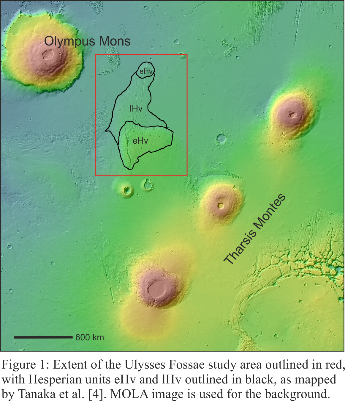
2. Methods
We used Context Camera (CTX) images, with a resolution of 6 m/pixel [3], to map all the faults in the Ulysses Fossae study site at a scale of ~1:250,000; mapping from Tanaka et al. [4] providing outlines for the three Hesperian geological units in the study area. Mars Orbiter Laser Altimeter (MOLA) data were used to create topographic profiles of select areas in Ulysses Fossae. The MOLA data was complemented by images from the High-Resolution Stereo Camera (HRSC), creating a Digital Elevation Model (DEM) with a resolution of 200 m/px [5]. Crater statistics derived from these three units with the “Cratertools” ArcMap tool and the Craterstats v.2 program [6, 7] were used to calculate absolute model ages.
3. Preliminary Results and Discussion
In total, we mapped 5,165 faults in Ulysses Fossae (Figure 2), with fault patterns ranging from linear to curved. Detailed analysis of the mapped faults, including investigating cross-cutting relationships, morphology, and azimuths, allowed us to divide the faults to into eight main fault populations (see Table 1). On the basis of strike, the majority of these populations reflect influence from local volcanic centers, as they display radial fault patterns to Olympus Mons, Pavonis Mons, and Ulysses Patera. One of the older populations, Population 2 (Table 1), dated to be Early Hesperian, appears to solely be the result of regional extension associated with the growth of Tharsis. The youngest fault population, Population 7, from the late Hesperian, consists of slightly curved grabens with a sigmoidal geometry and en echelon patterns, and appears to have formed by reactivation of the two oldest mapped fault populations.
Additionally, we acquired crater statistics for the geological units in the study area to calculate absolute model ages to aid in our understanding of the geological history of Ulysses Fossae. This analysis resulted in giving two of the units a potentially significantly younger, Amazonian age, than previously determined [4] see Fig. 2.

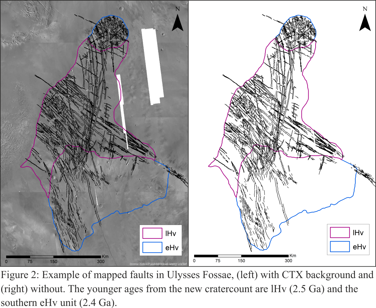
4. Summary and Conclusions
Our mapping resulted in the recognition and analysis of eight fault populations, which together suggest several stages of structural activity in the Ulysses Fossae region. Results from relative and absolute model age analysis so far indicate a complex history involving radial fault growth from the several surrounding proximal volcanoes (Olympus Mons, Pavonis Mons, and Ulysses Patera), later reactivation of pre-existing fault populations and some influence from the regional extension of the Tharsis rise.
Further investigations based on this initial work will include measuring extensional strain for the eight fault populations, and maximum displacement/length (Dmax/L) relationships for select study faults, with the data ultimately being intended to help in comparisons to other volcanic areas on Mars and other terrestrial planets.
Acknowledgements
To NASA for providing CTX and MOLA data, and ESA for HRSC data. Funding for this project was provided by the UK Research and Innovation (UKRI) Natural Environment Research Council’s (NERC) Doctoral Training Programme.
References
[1] Scott, D. H., & Dohm, J. M. (1990). Faults and ridges—Historical development in Tempe Terra and Ulysses Patera regions of Mars. Proceedings of the Lunar and Planetary Science Conference, 20, 503–513
[2] Fernández, C., & Ramírez-Caballero, I. (2019). Evaluating transtension on Mars: The case of Ulysses Fossae, Tharsis. Journal of Structural Geology, 125, 325–333.
[3] Malin, M, et al. 2007. Context Camera Investigation on board the Mars Reconnaissance Orbiter. Journal of Geophysical Research. 2007, Vol. 112.
[4] Tanaka, K. L., Skinner Jr., J. A., Dohm, J. M., Irwin, III, R. P., Kolb, E. J., Fortezzo, C. M., Platz, T., Michael, G. G., & Hare, T. M. (2014). Geologic Map of Mars (Scientific Investigations Map)
[5] Fergason, R. L., Hare, T. M., & Laura, J. (2018). HRSC and MOLA Blended Digital Elevation Model at 200m v2. [Map]. Astrogeology PDS Annex, U.S. Geological Survey.
[6] Michael, G.G. 2013. Planetary surface dating from crater size–frequency distribution measurements: Multiple resurfacing episodes and differential isochron fitting. Icarus. 2013
[7] Michael, G. G and Neukum, G. 2010. Planetary surface dating from crater size–frequency distribution measurements: Partial resurfacing events and statistical age uncertainty. Earth and Planetary Science Letters. 2010.
[8] Hartmann, W. K., & Daubar, I. J. (2016). Martian cratering 11. Utilizing decameter scale crater populations to study Martian history. Meteoritics & Planetary Science, 52, 493–510. https://doi.org/10.1111/maps.12807
[9] Michael, G. G., Kneissl, T., & Neesermann, A. (2016). Planetary surface dating from crater size‐frequency distribution measurements: Poisson timing analysis. Icarus, 277, 279–285. https://doi.org/10.1016/j.icarus.2016.05.019
How to cite: Shahrzad, S., Bramham, E., Thomas, M., Byrne, P. K., Mortimer, E., and Piazolo, S.: Deciphering the deformation history of Ulysses Fossae, Mars, using fault pattern analysis, Europlanet Science Congress 2021, online, 13–24 Sep 2021, EPSC2021-782, https://doi.org/10.5194/epsc2021-782, 2021.
Summary. We analyzed a global database of constraints on Mars paleolake size relative to topographic catchment area (aridity index) and found evidence for climate zonation during the late-stage river-forming climates. Aridity increased over time in southern midlatitudes, but wetter climates (semiarid to arid) persisted near the equator and in the northern midlatitudes.
1. Introduction. Mars’ geology records multiple eras of precipitation-fed water runoff (e.g. [1,2]). Regionally integrated Valley Networks (VNs) formed early, ~3.6 Ga. Later, river-forming climates created deltas and alluvial fans up to 1.1 km thick [3,4]. This late-stage river-forming era consisted of multiple, intermittent, river-forming climates [5]. Within craters, most of the fluvial sediment transport was driven by runoff from crater sidewalls. Crater-lake levels could also have been maintained by water conveyed from crater sidewalls (by overland flow or shallow groundwater flow) or alternatively, by deep sourced groundwater sourced from rain/melt recharge at ~102-103-km scales.
2. Results. To constrain late-stage river-forming climates, we carried out a global survey within large, young impact craters (n = 212; from [6]) for geologic constraints on crater lake size (i.e., aridity index) and lifetime. Survey results (Figs. 1-4) disfavor the hypothesis that late-stage lakes were caused by individually brief (<10 yr duration) wet events (for example, driven by impact kinetic energy). For example, we found 12 prefluvial/synfluvial impact craters. To accumulate so many prefluvial/synfluvial craters would have required ≥0.2 Gyr. 0.2 Gyr is far too long for river formation by localized impact-induced effects (consistent with [5]). We also surveyed constraints on late-stage lake area, A, and topographic catchment area, D (finding n = 118 basins with useful constraints). To constrain paleolake area A, we used flat crater-bottom deposits matching expectations for lake deposits, as well as the elevations of the following features: alluvial fan toes, scarp-fronted deposits interpreted as deltas, and channel-stop elevations, internal spillways, and a candidate shoreline. D/A – 1 (equal to the hydrologic X-ratio, XH ) is approximately equal in closed-basin hydrological steady state to the Aridity Index (AI) (ratio of potential evaporation to water discharge, neglecting runoff production on the lake and net of infiltration) [7,8]. Low XH corresponds to relatively large lakes and a wetter climate. If wet climates were brief, then because small sinks fill quicker than big sinks, XH should be higher for bigger craters (XH ∝ Rcrater2/3). To the contrary, our data indicate lower XH for bigger craters (Fig. 2a), with XH < 10 found mainly in large craters. This disfavors the scenario in which late-stage river-forming climates were powered by the greenhouse forcing from a single volcanic eruption, or the energy of a distant impact. Our results provide additional support for the inference (e.g., [3]) that an arid but essentially Earth-like hydrologic cycle fueled late-stage rivers.
Our aridity analysis shows that late-stage XH < 10 is less common S of 10°S (Fig. 2). This late-stage climate zonation might be caused by the effect on the global circulation and/or water cycle of latitudinal gradients in elevation. Elevation control on late-stage river abundance is consistent with elevation control on paleolake levels and on climate zonation. Climate zonation helps to understand the changes over Gyr timescales (that are revealed by our database) in the aridity index of paleolake basins. For early-stage Valley-Network era (~3.6 Ga), the typical XH reported lakes is XH,ancient = 5±2 ([7]; consistent with ref. [8]; but see also [9]). Late-stage XH was 7-38 (median fan toe constraint to median lake deposit constraint), corresponding to arid-to-hyperarid conditions, with deltas and overspill channels recording semi-arid conditions (median XH=4). These data indicate a climate trend, to more arid climate (our preferred explanation), or alternatively toward briefer wet events (not ruled out by our data), on global average. This global trend can be decomposed, taking account of climate zonation, into a shift where southern midlatitudes show a shift towards smaller lakes over time, but intermittent wet climates (semiarid to arid) persisted in the equatorial region and the northern midlatitudes.
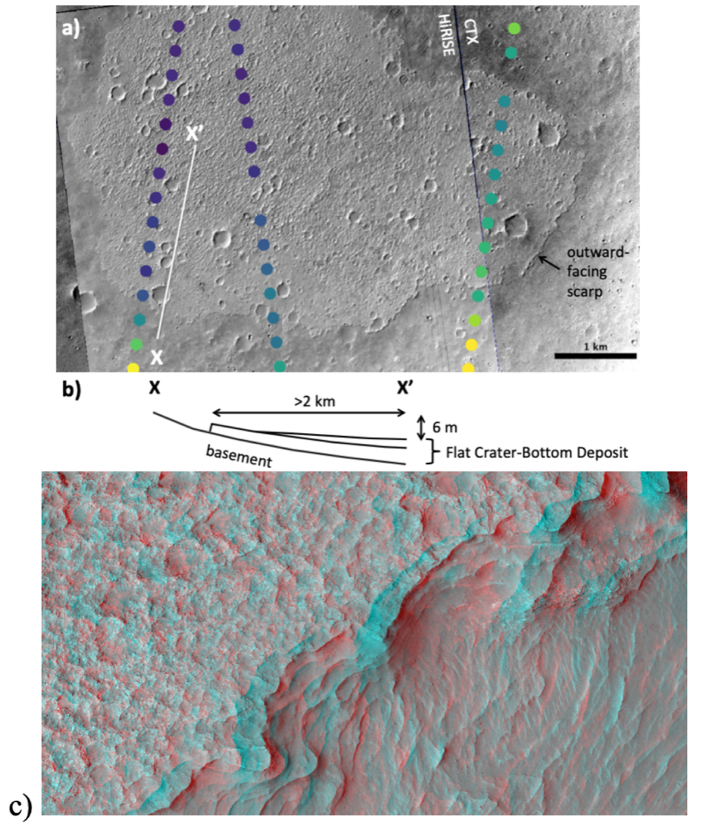
Fig. 1. (a) Example of a flat crater-bottom deposit (interpreted as a lake deposit). ESP_062496_1880. Color scale (MOLA) runs from -180 m (yellow) to ‑220 m (deep blue). (b) Sketch cross-section of profile X‑X’ in (a). (c) Anaglyph of the margin of a flat crater-bottom deposit (ESP_065480_1495), showing nearly-horizontal mid-toned layers exposed beneath the lighter-toned erosionally-resistant cap. 920 m across.
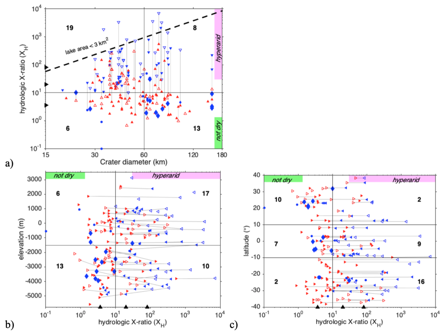
Fig. 2. Late-stage aridity constraints: (a) XH vs. crater diameter. Blue triangles=flat crater-bottom deposits (interpreted as lake deposits) (unfilled=candidate), blue diamonds = deltas/shorelines, blue circles = internal spillways, red filled triangles = alluvial fan toes, and red unfilled triangles = channel-stops. Numbers: # of constraints lying entirely inside a rectangular region. Gray lines connect lowest and highest constraint for a single basin. Black triangles correspond to aridity indices (from ref. [7]) for (from wet to dry) Great Basin wet period; Nevada, present; Death Valley, present. (b) XH vs. elevation. (c) XH vs latitude.
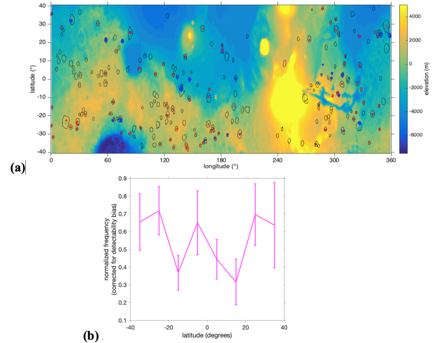
Fig. 3. (a) Survey map. Black contours outline the young geologic units (“AHi” from [6]) that were inspected for paleohydrology constraints. Symbols: as in Fig. 2. (b) Distribution of craters with paleohydrologic evidence with latitude (expressed as a fraction of the number of surveyed craters in that latitude band).
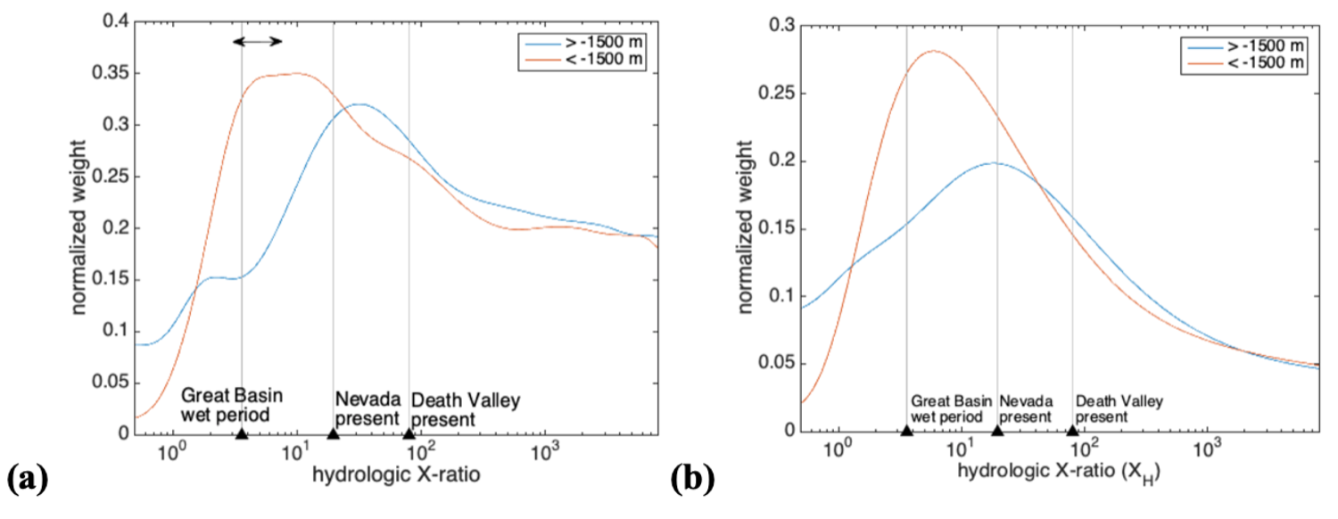
Fig. 4. (a) Kernel density estimate of late-stage XH changes with elevation. Double‑headed arrow corresponds to estimate for early-stage rivers (XH ,ancient = 5±2) from [7]. The modern-Earth aridity values shown by black triangles here are also from [7]. Log‑uniform prior on XH = {0.1, 104}. (b) As (a), but with a log-uniform prior on XH = {0.1, 1014}.
References:[1] Grant & Wilson, GRL 38, CiteID L08201 (2011).[2] Kite, Space Sci. Rev., 215:10 (2019).[3] Irwin et al., Geomorphology, https://doi.org/10.1016/j.geomorph.2014.10.012 (2015).[4] Kite et al., GRL 44, 3991-3999 (2017).[5] Kite et al., Science Advances, 5(3), eaav7710 (2019). [6] Tanaka et al., Geologic map of Mars:USGS Scientific Investigations Map 3292 (2014).[7] Matsubara et al., JGR 116, E4, E04001 (2011).[8] Stucky de Quay et al., Geology 48 (12): 1189–1193 (2020).[9] Fassett & Head, Icarus 198(1), 37–56 (2008).
Grants:NASA(80NSSC20K0144+80NSSC18K1476).
How to cite: Kite, E.: Billion-year trends in the aridity of river-forming climates on Mars, Europlanet Science Congress 2021, online, 13–24 Sep 2021, EPSC2021-345, https://doi.org/10.5194/epsc2021-345, 2021.
Introduction: What key processes modify “out of equilibrium” landforms (impact craters) on Mars and how do we model them quantitatively [1-8]? Amazonian-Late Hesperian craters display generally fresh and pristine morphologies. Noachian-Early Hesperian craters show fundamental morphological differences (e.g., general absence/subdued nature ejecta, elevated crater rim-crests being low or missing, shallower flat floors, missing central peaks, and often textured/grooved walls). These differences were interpreted to be due to relatively higher Noachian erosion rates attributed to landform degradation by rainfall (pluvial activity), in a warmer/wetter climate with a LN “climate optimum” resulting in fluvial erosion/VN [1-8]. Indeed, “Degraded craters are one of the main lines of evidence for a warmer climate on early Mars” [9]. Further analysis of 281 >20 km craters in two highland regions [9] confirmed earlier findings, revealing three classes: Type III: Fresh craters with ejecta/central peaks; Type II: Gently degraded with fluvial landforms/alluvial fans; Type I: Strongly degraded, without ejecta/central peak, with fluvial erosion. Type I were formed/degraded during the Noachian, Type II between EH-EA, and Type III formed subsequently. A sharp transition is seen between Types I/II, interpreted to indicate a rapid change in climate conditions [9]. New missions, discoveries, models and data analysis make it opportune to revisit/xplore Mars crater degradation and landscape evolution.
Perspectives on Noachian Geologic Sequence and History: A synthesis of sequence/timing of conditions on early Mars [10] showed 1) distinctive separation of EN basin-forming period from MN-LN during which no basins formed, 2) LN-EH when valley networks (VN) formed [11], unrelated to basins [12], 3) lack of correlation between phyllosilicates/VN formation.
Role and Legacy of Impact Basin Formation: Recent studies of impact basin effects on climate and EN surface modification show that the threshold diameter for radical atmosphere effects is in the basin-size range [13-14]; collective effects of basin-scale atmospheric/surface effects (ICASE) are: 1) globally distributed very high temperature rainfall; 2) extremely high (~2m/yr) rainfall/runoff rates; 3) significant degradation of crater rims, filling of interiors, regional smoothing; 4) significant influence on mineralogical alteration of the crust [14]. These major events impart a global legacy into the surface nature/morphology.
Models of Noachian Climate: Atmospheric general circulation models [15-16] suggest ~225K mean annual temperature (MAT), a distinctive alternative to the generally warm/wet/arid pluvial climate [1-8] implied by earlier models [1-8]; an adiabatic cooling effect predicts a “cold and icy highlands” [16] with snow/ice accumulating above ~+1km. VN, open/closed basin-lakes are attributed to transient heating/melting of snow and ice in the “icy highlands” [17-18]. The influence of substrate snow/ice on cratering and degradation [19-20] includes: 1) Amazonian-like double-layered ejecta/pedestal craters; 2) shallower underlying target-rock cavities in the, lower post-ice rims; 3) modification by rim-crest backwasting, ice melting and fluvial erosion. Removal of surface snow/ice could eliminate smaller craters, drastically modifying size-frequency distributions.
GCMs of a “warm/wet” climate (MAT ~275K)[21]: rainfall is limited in abundance/areal distribution, precipitation is snowfall-dominated, and highlands are <273K for most of the year. Thus: 1) VN/lakes should not form through rainfall-related erosion, 2) rainsplash/runoff crater degradation is not predicted, and 3) a northern ocean is improbable.
New Observational Data: Global crater-wall steepest-slope distribution was used to assess magnitudes of degradational processes with latitude/altitude/time [22]: total LN crater-wall degradation is very small, interpreted to mean that LN climate was not characterized by persistent/continuous warm/wet conditions. MRO-CTX [23] reveals evidence for crater-wall cold-based glaciation, top-down glacial melting, fluvial crater floor meltwater drainage/endorheic crater-floor lake.
Outstanding Questions: A full understanding of Noachian crater degradation clearly requires addressing the following questions: 1) What is the magnitude of the role of the impact flux and its effect on crater degradation and diffusional processes, and how does this change with atmospheric pressure? 2) In a warm and wet/arid climate, what was the intensity of the rainfall required for infiltration and what is the rate transition to runoff? How does this vary with atmospheric pressure and substrate? 3) What causes the abrupt change from highly degraded craters to much less degraded craters at the end of the Noachian? 4) What role do EN basin-related torrential rainfall processes have [24] on setting the stage for LN crater formation and degradation? 5) What role do explosive [25] and effusive [26] volcanism play in the resurface of craters and filling of crater floors? 6) How widespread is the evidence for Noachian glaciation [23] and what are the implications for crater modification and degradation state? 7) How do eolian processes vary with atmospheric pressure and how does this influence crater degradation with time? 8) Can the observed fluvial activity and open and closed-basin lake degradation and filling be explained by transient heating phenomena in an otherwise cold and icy climate?
References: 1. Craddock&Maxwell, 1990, JGR95, 14625; 2. Ibid, 1993, JGR98, 3452; 3. Craddock et al., 1997, JGR102, 13321; 4. Craddock&Howard, 2002, JGR107, 5111; 5. Forsberg-Taylor et al., 2004, JGR109, E05002; 6. Howard et al., 2005, JGR 110, E12S14; 7. Irwin et al. 2005, JGR110, E12S15; 8. Howard, 2007, Geomorphology91, 322; 9. Mangold et al., 2012. JGR117, E04003; 10. Fassett&Head, 2011, Icarus211, 1204; 11. Ibid., 2008, Icarus195, 61; 12. Toon et al., 2010, Ann Rev38, 303; 13. Turbet et al., 2019, Icarus335, 113419; 14. Palumbo&Head, 2018, MAPS53, 687; 15. Forget et al., 2013, Icarus222, 81; 16. Wordsworth et al., 2015, Icarus222, 1; 17. Head&Marchant, 2014, Antarctic Science26, 774; Fastook&Head, 2015, Icarus106, 82; 18. Palumbo et al., Icarus300, 261; 19. Weiss&Head, 2015, PSS117, 401; 20. Ibid., 2016, Icarus280, 205; 21. Palumbo&Head, 2018, GRL45, 10249; 22. Kreslavsky&Head, 2018, GRL45, 751; 23. Boatwright&Head, 2021, PSJ2, 1; 24. Palumbo&Head, this volume; 25. Kerber et al., 2013, Icarus 223, 149; 26. Whitten&Head, 2013, PSS 85, 24.
How to cite: Head, J. and Boatwright, B.: Revisiting Noachian-Hesperian Crater Degradation Processes and Potential Climate Effects, Europlanet Science Congress 2021, online, 13–24 Sep 2021, EPSC2021-426, https://doi.org/10.5194/epsc2021-426, 2021.
The Odd Lengthy Valleys of the Early Hesperian Volcanic Unit Mars. R. S. Bahia1, 1European Space Agency (rickbir.bahia@esa.int)
Introduction: Martian valley networks are evidence for surface run-off and past water cycles on ancient Mars [e.g. 1–3]. There is still great uncertainty in the duration, intensity and surface conditions that led to valley formation. However it is generally agreed that most formed as a result of precipitation-fed (most likely snowfall) fluvial [4] and subglacial melt water incision [5], with some forming via sapping erosion. Precipitation-fed networks have characteristics that resemble terrestrial systems; e.g., the valleys generally originate at or adjacent to drainage divides [6], some of which have numerous tributaries with drainage densities comparable to low-order terrestrial valley systems [3]. Subglacial valleys have large width-to-depth ratios and undulating long. profiles [e.g., 7]. Qualitative observational characteristics typical for subglacial channels are an abrupt source and termination, stepped long. profiles, a semi-uniform width and no meter scaled tributaries [e.g., 7].
Most valleys incise Noachian to Early Hesperian aged surface [e.g., 3], indicating this was the period of peak fluvial activity. The morphology of these valleys likely reflects the intensity and duration of fluvial activity at their time of formation, with Early Noachian to Mid-Noachian (4.15 – 3.85 Ga) networks draining into local lows and being relatively short (≤100 km long) and Late Noachian/Early Hesperian surfaces displaying regionally-integrated valley networks across the Southern Highlands, likely indicative of a peak in fluvial activity [e.g., 4].
In a recent valley mapping effort using High/Super Resolution Stereo Colour Imager (HRSC) images (~ 25 m per pixel), a small number of lengthy single-thread valleys, that a morphologically dissimilar than the majority of valley networks, were identified. This study aims to perform detailed morphological analysis of these valleys in order to better understand their origin. Here I present the initial observations of these valleys.
Data and Methods: Valley were identified in ESA Mars Express Orbiter – High/Super Resolution Stereo Colour Imager (HRSC) images (~ 25 m per pixel) and manually mapped using the polyline function within ArcMap 10.2.1, defined under analogous characteristics as those of previous studies [e.g., 3, 8]; i.e., sublinear features dividing into small branches upslope and become singular downstream whilst slightly increasing in size. CTX (Context Camera – ~5m per pixel) images were used to perform detailed morphological analysis. Drainage density was determined as the total length of valleys within a set radius of 235 km for each output raster cell (in accordance with [3]) using the ArcMap Spatial Analyst - Line Density tool.
A combination of HRSC digital elevation models (DEM) and the Mars MGS MOLA - MEX HRSC Blended DEM Global 200m v2 [9] was used to obtain elevation data. In order to determine the relative ages and geological settings of the mapped valleys, the Tanaka et al. (2014) digital global map of Mars was used [10]. The ages for these surfaces are determined from crater density counts.
Results: At present these valleys have been predominantly identified incising Early Hesperian aged units, specifically those with volcanic origins. The source and termination of these valleys is generally abrupt. They have almost no tributaries and are essentially comprised of one lengthy main valley. For example, the valley presented in Figure 1 has a main valley length of 332.2 km, a total valley length of 674.9 km, and very low drainage densities (max. 0.004 km-1). The branches of valleys that add to the main valley length (resulting in a higher total valley length) do not appear to be tributaries, but areas in which the main valley has become anastomosed and disconnected in areas due to ejecta blanket coverage and erosion. The width of this valley is relatively uniform down its profile (0.5 – 0.7 km), which is consistent for all valleys of this type. Additionally, reaches of the valley become inverted in topography, causing it to protrude from the surface when compared to the surrounding region. The valleys appear to divert around topographic features (e.g., craters).
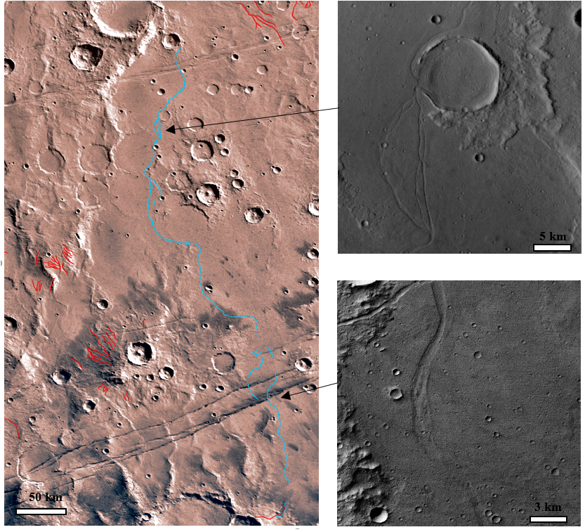
Figure 1. Example of lengthy valley (blue line) overlaid on Mars_Viking_MDIM21_ClrMosaic_global_232m. The red lines are those valleys mapped by Hynek et al. [2010]. In HRSC it can be seen that the valley is anastomose in regions and has areas where the valley is comparatively positive in relief compared to the surrounding material.
Discussion: At present the origin of these valleys is unclear. However, based on the fact that the valleys seem to flow around topographic features, e.g., craters, it would seem that they were formed by incision of a fluid. Whether this fluid was water (i.e., fluvial/subglacial) or lava cannot be confirmed at present. Additionally, these valleys are almost exclusively presence only in Early Hesperian volcanic units, indicating their origin or preservation is related to this unit. Examining these valleys in more detail will aid in determining the origin of these valley networks and gain insight into the surrounding conditions at their time of formation.
References: [1] Milton D. J. (1973) JGR, 78, 4037–4047. [2] Carr M. H. (1995) JGR, 100, 7479–7507. [3] Hynek B. M. et al. (2010) JGR, 115, 1–14. [4] Kite, E. S. (2019) Space Sci Rev., 215:10. [5] Galofre et al. (2020), Nature Geoscience, 13 (10). [6] Craddock R. A. and Howard A. D. (2002) JGR, 107, 1–31. [7] Galofre et al. (2018), Cryosphere, 12, 1461-1478. [8] Bahia R. S. & Jones. M (2020) Earth, Moons and Planets, 123, 45–59. [9] Fergason et al. (2017), LPSC XLVIII, Abstract 1563. [10] Tanaka et al. (2014), Planet. Space Sci., 95, 11–24.
How to cite: Bahia, R.: The Odd Lengthy Valleys of the Early Hesperian Volcanic Unit Mars, Europlanet Science Congress 2021, online, 13–24 Sep 2021, EPSC2021-784, https://doi.org/10.5194/epsc2021-784, 2021.
Most of the Martian fluvial valleys formed in the early period (around the Noachian-Hesperian boundary or before), but the formation durations are not well determined, however it would be important to understand as it is related to the climatic history and the reason for specific morphology of the Red Planet’s valleys. We estimated the formation duration for a hundred different sections of a small (~81 km long) Martian valley (called Tinto B, which is East of Palos crater and Tinro Vallis), using ArcMap and Excel software. We used the HRSC DTM (Digital Terrain Model), which was resampled from the resolution of 50 m/px to 100 m/px, because the used THEMIS TI dataset (used for grain size estimation) has a 100 m/px resolution. The visual morphological analysis we used the CTX images. For the calculation we considered the cross-sectional profile of the valley as a trapezoid shape and calculated the hydraulic radius for it and used several hydraulic variables, like average flow velocity, bedload transport rate, sediment and flow discharge [1], slope of energy grade line. For the formation timescale calculation the Meyer-Peter and Muller bedload transport equation [2] was used. For the sediment grain size estimation we used the THEMIS TI dataset and calculated the shear stress and the Shield parameter from it [3]. The bed of the valley is covered with aeolic sand, which does not represent the grain size of the eroded bedrock, which probably took part in the original formation process. For this reason we sampled the grain size from exposures on both sides of the valley walls, where the original bedrock represented to the best approximation and continuously. The main aim of the work is to compare the different sections of the analysed valley by the final assumed age and different variables and morphology. The detailed morphology analísation comes from the previously made erosion-accumulation results [4] and the visual analysis of the valley. From the given section results the median formation time scale of the valley can be calculated also. With this method the Martian valleys can be comparable with the terrestrial mars-analog valleys after the same calculations. The estimated formation timescale of the whole valley will be compared with the result of the crater size frequency distribution based statistically estimated age of the valley bed.
References:
[1] - M. R.T. Hoke, B. M. Hynek, G. E. Tucker, Formation timescales of large Martian valley networks, Earth and Planetary Science Letters, 2011, Volume 312, Issues 1–2
[2] - M. Wong, G. Parker, Reanalysis and correction of bed-load relation of Meyer-Peter and Muller using their own database, J. Hyrdaul. Eng, 2006, pp. 1159-1168
[3] - L. K. Fenton, J. L. Bandfield, A. W. Ward, Aeolian process on Mars: atmospheric modeling and GIS analysis, Journal of Geophysical Research, 2003
[4] - V. Steinmann, Á. Kereszturi, L. Mari, Geomorphological analysis of Tinto-B Vallis on Mars, Hungarian Geographical Bulletin, 2020, pp 333-348
How to cite: Steinmann, V. and Kereszturi, Á.: Formation timescale model for a small sized Martian fluvial valley, Europlanet Science Congress 2021, online, 13–24 Sep 2021, EPSC2021-212, https://doi.org/10.5194/epsc2021-212, 2021.
1. INTRODUCTION
The purpose of this work is to analyze the formation process of a steep fan-shaped deposit in the Coprates Catena region, using a depth-integrated model. The origin of this fan is however uncertain. Probably a clay-water mixture flowed along a long valley and entered a deep trough giving rise to a stepped fan. According to local morphotectonics [3,7] groundwater-related processes could have been active from Hesperian to early Amazonian, thus implying favorable environmental conditions for the mudflow occurrence during that period.
These types of phenomena are very sensitive to topography, geological and environmental conditions. In absence of erosion and other weathering factors, and once the deposits are formed, they may remain unaltered during millions of years. Therefore, the analysis of these depositional processes may assist us in better understanding the geological and climatological history of Mars.
2. METHODOLOGY
The regional morphology at Coprates Catena has been widely studied and it is geologically well characterized, thus allowing the topographic reconstruction of the area. Some previous works [1,3,8] suggested that the stepped fan-like-structure formation was probably carried out in several phases, with a time-lapse in between. Our study focuses on the last phase of this discontinuous event, when the upper part of the fan was deposited.
The methodology proposed herein consists of: (i) Reconstruction of the channel-fan formation by means of an iterative process using both mapping and mechanical modeling [4], and (ii) back-analysis of the alluvial fan depositional process using a numerical model.
In order to carry out the numerical study of the aforementioned depositional process, the authors propose the use of the depth-integrated model described in [5] based on the depth-integrated Navier-Stokes equations, also known in some disciplines as the Shallow Water Equations. These equations are integrated in space using the Finite Element Method [9] and in time using the two-steps Taylor-Galerkin algorithm [2,6]. The resulting model allows the dynamic simulation of landslides and flowslides, such as granular flows, debris flows or mudflows, providing the arrival time and run-out of the flow, as well as its final depositional volume and shape. The model includes some constitutive models, such as newtonian fluids (laminar and turbulent), Bingham fluids and frictional fluids as well as different bottom-friction laws.
The proposed model requires the following information as input:
(a) Reconstructed topography:
Before running the numerical model over real surficial data, it is necessary to reconstruct the shape of the terrain to a previous state, before the alluvial fan was formed. In order to do that, an iterative process is proposed [4]. Running the model [5] on an initial reshaped surface (with the channel filling volume as the starting condition), new information is obtained to enhance the reconstruction, thus starting an iterative process: alternation between reshaping the topography and running the model is performed until the result of the latter fits the shape and characteristics found in the initial unaltered topography, before the depositional fan-like structure was formed. This reconstructed topography is then interpolated in a non-structured computational mesh of 206702 linear triangles and 103487 nodes (Figure 1).
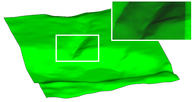
Figure 1: Reconstructed topography and detailed view of the computational mesh
(b) Mobilized mass:
After topographic reconstruction, the mobilized mass of material must be determined. In order to do that, and, based on what can be identified in the imagery, the channel is filled by the fan-equivalent volume up to a knickpoint (Figure 2).
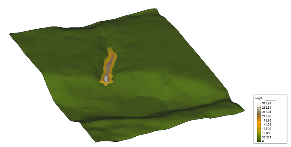
Figure 2: Mobilized mass (initial condition for t = 0 s)
(c) Type of material:
The type of material involved in the process is given by the parameters of the considered rheological law. These parameters must be determined using a back-analysis technique and thus comparing the final deposited volume, shape, slope and flooding area with the observational data.
3. RESULTS
In the present study a set of simulations have been accomplished using different rheological laws (newtonian, frictional and Bingham fluids) getting the most suitable result according to the current observations of the area for a Bingham fluid of density 1747 kg/m3, viscosity 0.118 Pa s and yield stress of 3 MPa. This result is compatible with a mudflow, probably a clay-water mixture of kaolinite type with a water content of about 53%. The final depositional material is shown in Figures 3 and 4.
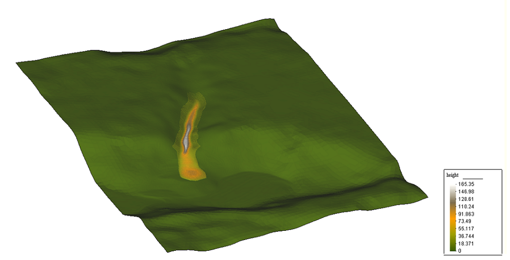
Figure 3: Final state of the sliding mass ( t = 21500 s = 5.97 hours)
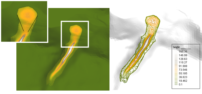
Figure 4: Plan view and detailed fan-like structure
4. CONCLUSIONS
We have proposed and applied a methodology for the reconstruction of a depositional process in ancient Mars to the particular case of an alluvial fan at Coprates Catena in Valles Marineris. Geomorphological reconstruction of the area of study has been accurately accomplished so that the initial conditions for the triggering event have been determined. A depth-integrated model using the Finite Element Method has been used in order to carry out a back-analysis of the event. The obtained results are in agreement with the observational data and are consistent with the geological characterization of the surrounding area. Therefore, numerical modeling of these processes is proposed as a powerful tool providing a better understanding of the geological and environmental conditions of ancient Mars.
ACKNOWLEDGEMENTS
A.M. is funded by the Project "MarsFirstWater", European Research Council Consolidator Grant no. 818602. T.M. was founded by the grant JAEIntro-2020-CAB-03. The authors thank the Agencia Estatal de Investigación (AEI) project no. MDM-2017-0737.
REFERENCES
[1] Di Achille et al. (2006). Geophysical research letters, 33(7).
[2] Donea (1984). Inter. J. Numer. Methods Eng. 20(1): 101-119.
[3] Grindrod et al. (2018). Icarus, 307, 260-280.
[4] Molina, Herreros, Martínez-Pérez et al. (2021). EPSC2021-129.
[5] Pastor, Herreros et al. (2009). Engineering Geology, 109(1–2): 124-134.
[6] Peraire et al. (1986). Inter. J. Numer. Methods Eng., 22: 547–574.
[7] Salese et al. (2019). Journal of Geophysical Research: Planets, 124(2), 374-395.
[8] Weitz et al. (2006). Icarus, 184(2), 436-451.
[9] Zienkiewicz et al. (2005). The Finite Element Method. Vol. 1-3. 6th Ed. Butterworth-Heinemann.
How to cite: Herreros, I., Molina, A., Martínez-Pérez, T., Bacallado, A., Mata, S., and Gómez, B.: Alluvial fan at Coprates Catena in Valles Marineris, Mars: new modeling insights., Europlanet Science Congress 2021, online, 13–24 Sep 2021, EPSC2021-116, https://doi.org/10.5194/epsc2021-116, 2021.
Introduction: Inverted channel belts have been recognized on Mars [1,2]. A channel belt represents an extensive fluvial package of sediments which usually formed from lateral migration and aggradation of a river over time [3]. An inverted channel belt is created because the sediment package developed an inversion of relief as some sections were infilled by, or formed from, a more resistant material than the neighboring terrains. The surrounding terrains, less resistant to the erosion were removed, leaving the more resistant sediments upstanding [3] and often organized into characteristic sinuous ridges. This process implies that the fluvial system that deposited the material associated with the channel belt structure must have been active and stable for a long time (about 105-107 years [1]), and then a major change occurred, moving from a period of deposition to a period of erosion. The discovery of these features on Mars could have a major role for the dry-cold versus warm-wet climate debate [4]. Here, we present results from a mapping study in support of an inverted channel belt system developed within the degraded and partially buried Arago crater,in south-east Arabia Terra.
Methodology: HRSC-MOLA DEM [5] and CTX mosaic [6,7] data were ingested into ArcGIS software to study the general context of the study area, and to assist analysis of stratigraphy. A digital morphostratigraphic map (scale 1:10,000) was constructed using the available HiRISE [8] image and represents our interpretation of the area. Units are divided into three main groups:(i) The ‘Ridge formation‘ (units with strong correlation to the main ridges and likely represent fluvially-deposited material), (ii) ‘Basal units, (terrains stratigraphically below the inverted systems, or unrelated to them), (iii) ‘Miscellaneous units’ (heterogeneous materials, erosional remnants). The focus of the mapping was to determine the relationships between the sinuous ridge segments and the proximal surrounding terrains.
Observations: Arago crater is in Middle Noachian [9] terrains, and is bordered by valley networks [10] at north and south, suggesting that the area was influenced by fluvial processes. Water probably filled Arago crater and the surrounding topographic lows, evolving into temporary paleo-lakes or basins. The studied system is found at the south-west of Arago crater and here we refer to it informally as Arago Dorsum. Arago Dorsum is a continuous, branched, inverted network. Each branch of the system presents a variation in cross section style, expressing a different erosional stage[11]. The branches present smooth or cratered upper surfaces, and the longest segments are connected to smaller, secondary ridges. The Arago Dorsum ridges are upstanding and set within a low-reliefelevated material, demonstrating that they are resistant to erosion. The ridges are both laterally and vertically separated, organised in a multilevel structure.
Results: In the Ridge Formation sequence (Fig. 1), the main mapped ridges units (Urf 1-2, Srf 1-2, Lrf 1-2-3) are set at different stratigraphical levels and distributed within both Marginal units (Mrf 1-2) and the lower Transitional units (Trf 1-2-3), which correspond to ~65 m of vertical deposits (Fig. 2). Mapping allowed the recognition of other fine-scale features including: (i) more resistant thin layers visible at the flanks of the main ridges, or distributed in the Marginal units, (ii) the presence of smaller and secondary sinuous ridges which connect and disconnect at different stratigraphical levels, (iii) the presence of polygonal networks, possibly connected with secondary groundwater infilling, (iv) boulders and mass wasting falling from the ridges.
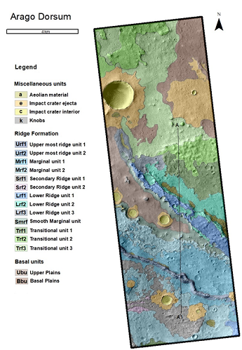
Figure 1: Gemorphic map of the “Arago Dorsum” system. The track A-A1 is presented in Fig. 2.
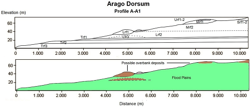
Figure 2: Morphostratigraphic profiles(vertical exaggeration x 20) presenting the main mapped units (indicated with labels on the top) and the interpretation (bottom). The cross-section A-A1 track is indicated in Fig. 1.
Interpretation: Based on the recognised fine-scale features, ridge morphologies, distribution and relationship of the mapped units, we interpret Arago Dorsum to represent the expression of an aggrading fluvial system, now preserved as an inverted channel belt. Specifically, the alternation of more resistant (ridges and layers) and the less resistant (Marginal-Transitional) units is in line with a flood plain sequence with preserved overbank deposits and discrete or stacked channel bodies. The three main ridges identified in the mapping area represent three periods of deposition. As other ridges have been recognised at CTX observation scale, the sequences reported here include only part of the Arago Dorsum stratigraphy, which may be even more complex, and probably even more long lived.
Conclusions: We interpret the Arago ridge system to be fluvial in origin, preserved in positive relief and now modified by differential erosion. Our observations and mapping reveal the inverted channel candidate to be the sedimentary deposits of an extensive aggradational fluvial channel-belt system, probably active in the Mid-Noachian. Valley networks inflowing Arago crater possibly supplied the channel-belt. There is a succession with at least 65 m vertical thickness of fluvial sediments here. Aram Dorsum, in western Arabia Terra (over 2000 km distance and over 1500 m elevation difference from Arago) presents very similar characteristics, including (i) age, (ii) morphology, (iii) vertical thicknesses of sediments, and (iv) the presence of polygonal networks developed in the units associated with the ridge development. These similarities suggest that similar thicknesses, volumes, and secondary processes (burial, erosion, groundwater alteration) of mid-Noachian fluvial sediments may be extensive and common in Arabia Terra. The presence of two (probably more) inverted channel belts, dated to the Mid-Noachian provide supports a past climate with widespread precipitation across Arabia Terra during this period.
References:[1] Balme et al.,(2020), JGR Planets,https://doi.org/10.1029/2019JE006244. [2] Liu et al.,(2020), Earth and Planetary Science Letters, https://doi.org/10.1016/j.epsl.2021.116854. [3] Hayden et al.,(2019), Icarus, https://doi.org/10.1016/j.icarus.2019.04.019.[4] Wordsworth et al.,(2016), Annual Review of Earth and Planetary Sciences, 10.1146/annurev-earth-060115-01235.[5] Fergason et al.,(2018), Astrogeology PDS Annex, U.S. Geological Survey. http://bit.ly/HRSC_MOLA_Blend_v0. [6] Dickson et al.,(2018), LPSC, 2480. [7] Malin et al., (2007), JGR Planets10.1029/2006JE002808. [8] McEwen et al.,(2007), JGR Planets, https://doi.org/10.1029/2005JE002605. [9] Tanaka et al.,(2014), GeologicMap of Mars: USGS Scientific Investigations SeriesMap 3292, scale 1:20,000,000, pamphlet 43 p. [10] Hynek et al.,(2010), Journal of Geophysical Research, https://doi.org/10.1029/2009JE003548. [11] Mirino et al.,(2020), LPSC, 1500. [10] Mirino et al.,(2020), LPSC 1492.
How to cite: Mirino, M., Balme, M., Fawdon, P., and Grindrod, P.: Evidence for a channel belt development within the Arago crater on Mars., Europlanet Science Congress 2021, online, 13–24 Sep 2021, EPSC2021-311, https://doi.org/10.5194/epsc2021-311, 2021.
- INTRODUCTION
Mars’ surface shows evidence of a decreasing geological activity over the years, leaving some geologic structures almost intact during the Amazonian era. This geologic age is characterized by the dry and inert conditions that can be found today. However, water-related features like channels and deltas prove that Mars was wetter and more active in previous eras, at least for brief periods. The study of surficial images and topographic data compared with analog structures on Earth allows us to infer the nature of these events. However, some processes are difficult to constrain and observations are not enough to answer some fundamental questions. Mechanical modeling applied to geological processes emulation is becoming increasingly powerful with the development of technology and new numerical solutions. Here we propose the iterative combination of both techniques, topographic reconstruction by mapping and mechanical modeling (detailed in [3]), to provide a better constraint for past surficial processes on Mars.
- METHODOLOGY
Before running numerical modeling over real surficial data, it is necessary to reconstruct the previous shape of the terrain. Even with a profound knowledge of the geologic history of the study area, some assumptions have to be made. Although the general shape of ancient features on Mars is still preserved, ulterior modifications may hinder proper modeling. Impact, tectonic, and gravitational processes alter original stream beds; aeolian deposits hide these channels’ original depth and shape.
We start reshaping the contours to reverse the terrain mobilized by the process to be studied, helped by what can be identified in the imagery. In this case, we remove the fan and fill the channel until a knickpoint [4]. To support the assumption that both the fan and knickpoint are coetaneous, we compare the volume of material of both reshapings. Running the model [3, 5] on the reshaped surface (with the channel filling volume as the starting condition), new information is obtained to enhance the reconstruction, starting an iterative process. The alternation between reshaping the topography and running the model until the result of the latter fits the shape and characteristics found in the initial unaltered topography allows tuning the topography. More than one hypothesis can be tested, providing insights during the iteration process itself.
Our testing case is a fan system found in Coprates Catena (14º 59’ S; 60º 15’ W) [1, 2, 4]. This structure shows more than one differentiated formation stage, according to slope variations, which was supported by previous studies (e.g., [2]). We hypothesize that initially, the material was deposited over a water body, producing a flat and extensive delta. The much steeper and concealed remaining fan was produced during a later episode(s), flowing this time into a dry surface on top of the previous delta. The channel and the outflow’s surface displayed a few modifications. The tectonics related to the Coprates horst/graben system acted after the channel/fan creation, producing several shrinks and faults that alter their shape. The reconstruction of those features has to be done without overly altering the original shape of the surface in order to provide a valid input for the mechanical modeling.
- RESULTS
The first step was to remove the upper part of the fan and fill the channel for the starting condition for the model (Figure 1B and 1C). When it was first run, the material flowed into a shrink instead of accumulating where the fan was. Those collapses likely postdate the fan deposition, as were identified in the images (Figure 1A). In later runs, the fluid found other obstacles identified in the imagery, as landslides along the channel. When all those flow impediments were removed, a fan with a resemblance to the observed one was obtained (Figure 1D, [3]). We tested different materials, water contents, and slopes; finding that this upper part of the fan is compatible with a kaolinite mudflow, with a water content of about 53% [3].
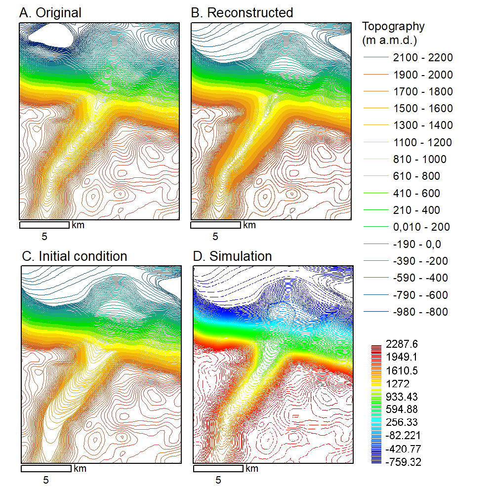
Figure 1. (A) HRSC derived topography (20m contours) of the fan (14º 59’ S; 60º 15’ W), (B) reconstructed topography previous fan formation, (C) reconstructed initial condition, and (D) result of the numerical model simulation [3].
- CONCLUSIONS
This workflow, through reconstruction of real data and application of a mechanical modeling, proved effective to simulate and constrain the formation of a channel-fan system on Mars. Our next step is to simulate the delta phase beneath this structure, and test if it is compatible with the deposition over a water body. This will allow us to refine this iterative process and test its capabilities for later application to other examples.
- ACKNOWLEDGEMENTS
A.M. is funded by the Project ‘MarsFirstWater’, European Research Council Consolidator Grant no. 818602. T.M. was founded by the grant JAEIntro-2020-CAB-03. The authors thank the Agencia Estatal de Investigación (AEI) project no. MDM-2017-0737 Unidad de Excelencia ‘María de Maeztu’.
- REFERENCES
[1] Di Achille, G., Ori, G. G., Reiss, D., Hauber, E., Gwinner, K., Michael, G., & Neukum, G. (2006). A steep fan at Coprates Catena, Valles Marineris, Mars, as seen by HRSC data. Geophysical research letters, 33(7).
[2] Grindrod, P. M., Warner, N. H., Hobley, D. E. J., Schwartz, C., & Gupta, S. (2018). Stepped fans and facies-equivalent phyllosilicates in Coprates Catena, Mars. Icarus, 307, 260-280.
[3] Herreros, M.I., Molina, A., Martínez-Pérez, T., Bacallado, A., Mata, S., Gómez, B. (2021). Alluvial fan at Coprates Catena in Valles Marineris, Mars: new modeling insights. EPSC2021-116.
[4] Weitz, C. M., Irwin III, R. P., Chuang, F. C., Bourke, M. C., & Crown, D. A. (2006). Formation of a terraced fan deposit in Coprates Catena, Mars. Icarus, 184(2), 436-451.
[5] Pastor, M., Herreros, I., Fernández Merodo, J.A., Mira, P., Haddad, B., Quecedo, M., González, E., Alvarez-Cedrón, C., Drempetic, V. (2009). Modelling of fast catastrophic landslides and impulse waves induced by them in fjords, lakes and reservoirs. Engineering Geology, 109(1–2): 124-134.
How to cite: Molina, A., Herreros, I., Martínez-Pérez, T., Mata, S., and Gómez, B.: Reconstructing a Martian channel-fan formation iteratively with mapping and mechanical modeling, Europlanet Science Congress 2021, online, 13–24 Sep 2021, EPSC2021-129, https://doi.org/10.5194/epsc2021-129, 2021.
Deltas are important landforms in planetary research and exploration because they indicate past fluvial activity, contain a sedimentary-record amenable to study, and have the potential to store past signs of life. As exploration missions are searching for (ancient) biomarkers, deltas are targets of interest. Therefore, it is important to understand the differences between deltas on Earth and Mars, so we can adjust our expectations of the past conditions and stratigraphy that we derive from the visible morphology. Furthermore, enhanced understanding of the effects of gravity can improve our estimations about past flow conditions and the duration of fluvial activity in certain areas. This eventually leads to a better understanding of the fluvial history of Mars and improved selection of target locations with the highest probability of preserved biosignatures.
To research the effect of gravity on deltas, we use a 2D hydro-morphodynamic numerical model that simulates the flow of water, transport and deposition of sediment, and the evolution of topography. We use the software Delft3D, developed by Deltares research institute (the Netherlands). This software is typically used for river and coastal systems on Earth, but we adapted the software by identifying all explicit and implicit dependencies on gravity, so it can also be used for deltas on Mars. The model set-up consists of a straight channel flowing into a sloping basin. The inflow channel is 200 m wide and the water depth is 3 to 10 m, depending on the model scenario. This results in discharges of about 1000 to 2500 m3/s. We impose two different grain sizes, namely a coarse fraction, transported as bedload, and a fine fraction, transported in suspension.
Our preliminary results show that gravity affects fine sediments stronger than coarse sediments, because of the difference in transport mode. For example, reduced gravity significantly slows down suspended sediment settling, while bedload transport is affected less. We expect that this will result in a different delta stratigraphy. This process is in addition to the effect that gravity has on water and sediment fluxes; lower gravity results in a smaller water discharge, while sediment transport is enhanced, with all else held equal. With our modelling efforts, we aim to further investigate the morphological results of these effects.
How to cite: Braat, L. and Lamb, M.: Effects of Gravity on Delta Morphology and Stratigraphy, Europlanet Science Congress 2021, online, 13–24 Sep 2021, EPSC2021-539, https://doi.org/10.5194/epsc2021-539, 2021.
Introduction: Numerous inverted fluvial channels occur on the surface of Mars [e.g. 1, 2, 3], and are found mainly in Late Noachian-Early Hesperian terrains [e.g. 6], and often within Arabia Terra [e.g. 1, 3]. A well-studied example is Aram Dorsum, a sinuous branched ridge interpreted as an inverted channel belt [7]. Sub-units within Aram Dorsum present a strong association with different types of decameter-scale, polygonally-patterned terrains:(i) Narrow-Fracture polygons, (ii) Wide-Fracture polygons, (iii) Narrow-Ridge polygons, (iv) Vein-like ridges, and (v) “meter-scale” polygons [7]. The mapping of the Aram Dorsum system shows that these types of polygons present both a distinct spatial distribution and a consistent stratigraphic pattern[7]. Developing a better understanding of the possible causes (local or regional) and formation processes of these polygonal terrains may offer an opportunity for a deeper understanding of the processes involved in inverted channel formation and development. We performed a regional survey within Arabia Terra to identify similar polygonal terrains and morphologies associated with other inverted systems. The main focus was on determining whether these polygon types are present within other terrains associated with inverted channels on Mars, and determine if the spatial/stratigraphic distribution observed in Aram Dorsum is consistent across the region.
Method: A database of inverted channels systems in Arabia Terra [8]was compared with HiRISE (25 cm/pixel, [9]) and CTX (6 m/pixel, [10]) image coverage using ArcGIS software. 205 HiRISE images were used for the identification of the polygonised terrains (observation-scale 1:2000). The observations have been made for all the inverted channels which were covered by at least one HiRISE image (Fig.1a). The result of the survey was a new database of polygonal terrain types associated with inverted channels, to which a simplified Aram-like morphological classification division was also applied (Fig.1b).
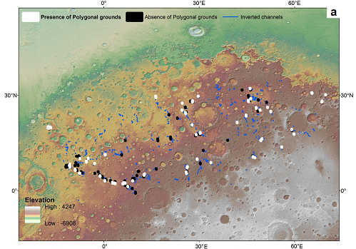
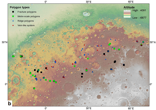
Figure 1: a-Studied HiRISE images which cover part of inverted channels(blue lines [8]). White colours indicate presence of polygonal-grounds. Black colours indicate absence of polygonal-grounds. b-Distribution of Aram Dorsum-like polygonal terrains.
Results: From the regional survey, Aram Dorsum-like polygons have been observed in association with many of inverted channels covered by HiRISE images found in Arabia Terra (Fig.2). 100 HiRISE images (out of 205 observed) have shown at least one polygonal type. The polygons have been found mainly associated with the main ridge itself or with the surrounding material adjacent to the inverted feature. Some materials close to the inverted channels may be characterised by only one type of polygonal morphology, and in this case fracture polygons or narrow ridge polygons are the most common types. Some examples of inverted channel deposits contain several types of polygonal features and it is difficult to define when a given type of polygon ends and another type begins. From the regional survey it was difficult to define a unique stratigraphic relationship between the polygonal terrains, and several inverted channels in Arabia Terra present unique morphologies and stratigraphy. However, a trend has been observed: fracture polygon types with clear morphology are usually found on top of the inverted channel, within erosional windows where the ‘capping unit’ has been removed, or on the closest associated materials. Narrow ridges or Vein-like polygons are usually developed within surrounding materials or sometimes in the lower parts of the main ridge (where exposed).Meter-scale polygons, or densely polygonal terrains, were found in proximity of craters linked to the inverted channels, or they have been observed between other polygonal fractures and between the narrow ridges polygons.
Interpretation: The Polygonal terrains have been observed in proximity to inverted channel features, on top of the ridge, along the flanks and within ridge-related materials (sometimes interpreted to be overbank deposits [7]) which could be distributed within the inverted channels in erosional windows. The identification of the same types of Aram Dorsum-like polygonal features in so many areas in Arabia Terra suggest that a common phenomenon could be found to explain their formation and development within these fluvial deposits. The persistence of the spatial distribution and a regional stratigraphical trend suggest a connection with the physical proprieties (e.g. grain size, induration, thickness) of the inverted channel deposited materials (fluvial origin) and their response to either (i) a regional stress, if the polygons formed underground as joints, or (ii) a surface process such as desiccation, thermal contraction or possibly a combination of the two. HiRISE images, selected in other areas with no inverted channels have been also checked to evaluate if such a fine-scale polygonal features could be distributed also somewhere else not in association with the inverted channel bodies. Based on preliminary observations on 10 HiRISE samples (randomly chosen) we have not been able to identify these small-scale polygonal terrains. However, since dust and impact materials were present, the survey will be expanded in future studies.
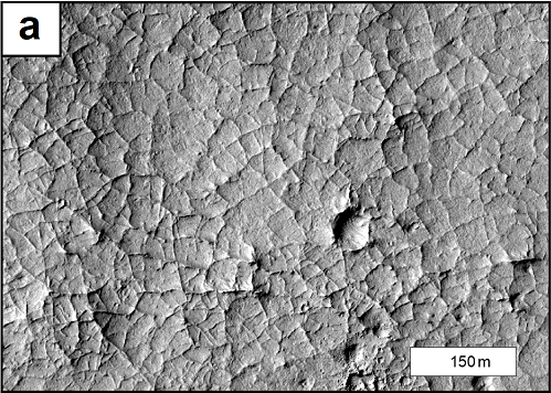
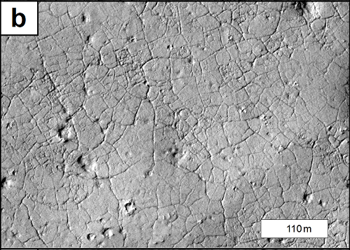
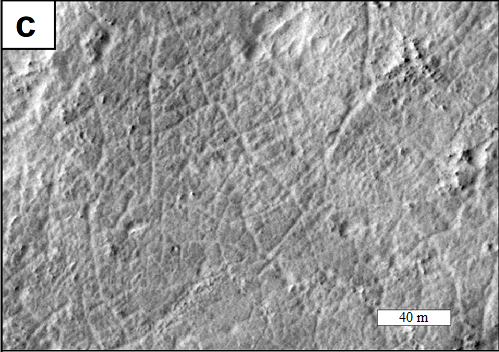
Figure 2: Example of Aram Dorsum-like polygonal terrains found in Arabia Terra region. a- Narrow ridge polygons, b- Wide fracture polygons, c- Meter-scale polygons (small domes) and Narrow fractures polygons.
Conclusions: Many other Aram Dorsum-like polygonal terrains have been observed and mapped in and around inverted channels in Arabia Terra, suggesting that inverted channels are likely to be observed associated with this type of polygonised terrains. A general spatial-stratigraphical trend has been observed, but deeper studies on selected candidates are necessary to confirm this. We will therefore perform more detailed morphological mapping choosing the a variety of inverted channel candidates in the area to further explore this possibility. More HiRISE images not associated to inverted channel bodies are also going to be controlled.
References: [1]Davis et al.,(2016), Geology, G38247.1. [2]Williams et al.,(2013), Icarus 225:308- 324. [3]Chuang & Williams,(2018), Journal of Maps, 14:2, 652-660. [4]Williams et al.,(2013), Icarus 225:308-324. [5]Williams et al.,(2007), Utah Geological Association, pp. 221-235. Salt Lake City, Publication, 36. [6]Tanaka et al.,(2014), Geologic Map of Mars: USGS Scientific Investigations Series Map 3292, scale 1:20,000,000, pamphlet 43 p. [7]Balme et al.,(2020), JGR Planets, https://doi.org/10.1029/2019JE006244. [8]Mirino et al.,(2020), LPSC 1492. [9]McEwen et al.,(2007), JGR Planets,https://doi.org/10.1029/2005JE002605. [10]Malin et al.,(2007), JGR Planets, 10.1029/2006JE002808.
How to cite: Mirino, M., Balme, M., Fawdon, P., and Grindrod, P.: Polygonal terrains associated with inverted channels in Arabia Terra, Mars., Europlanet Science Congress 2021, online, 13–24 Sep 2021, EPSC2021-332, https://doi.org/10.5194/epsc2021-332, 2021.
Abstract: The Medusae Fossae Formation (MFF) is an enigmatic sedimentary unit in the equatorial region of Mars with an uncertain formation process and age [1, 2]. Due to the heavily wind-eroded surface, it is difficult to determine the age of the MFF using existing crater count data and a one-parameter model based on the crater size-frequency distribution function [2, 3]. In our study, we used Context Camera (CTX) crater counts of 14 sites near the Medusae Fossae Formation, and other young equatorial units, to create a new two-parameter probabilistic model that estimates both age and erosion rate (β) by treating cratering as a random Poisson process. Our model predicts that the Central Medusae Fossae Formation and the top of Aeolis Mons (otherwise known as Upper Mount Sharp) have older ages (>1.40 Ga) and lower erosion rates (<650 nm/a), whereas East Medusae Fossae, Far East Medusae Fossae, Aeolis Planum, and Eastern Candor have younger ages (<0.740 Ga) and higher erosion rates (>740 nm/a). In addition to estimating ages consistent with previous studies, our new model also provides a better picture of how locations with higher rates of erosion are predicted to have younger best fit ages, and MFF locations with lower rates of erosion are predicted to have older best fit ages.
Methods and Results:
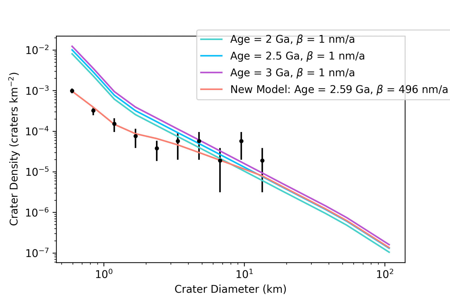
Fig 1. Crater density distribution (black points) corresponds to site 4B: Central Medusae Fossae 2B. On the left, we see that all three lines with negligible rates of erosion (β = 1 nm/a) overestimate the crater density for bins with small crater diameters, whereas including erosion rate in our new two-parameter model allows for a better fit.
We developed a new two-parameter model that uses crater count data to estimate a best fit erosion rate and age for each site. For sedimentary rocks on Mars, one-parameter (age-only) models typically predict an overabundance of small craters [4], as seen in Fig. 1. Our study region included 14 sites with boundaries based on USGS geologic map [5] and radargrams [6] (Fig. 2). We used manually counted craters within each of the 14 sites and divided the craters into 16 bins with crater diameters 0.5-128 km (based on [7]).
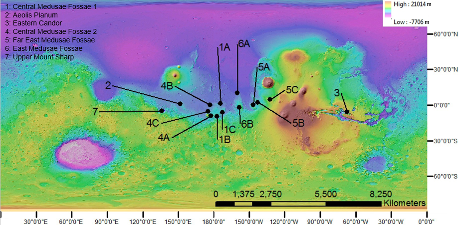
Fig. 2 Location of all 14 sites including Medusae Fossae Formation, Upper Mount Sharp, and Eastern Candor. Colors indicate MOLA topography in meters.
By contrast to [8], who created a two-parameter model using a Monte Carlo method, we treat cratering as a random Poisson process in order to apply a probabilistic model to find the best fit age and erosion rate β. This model considers each region’s surface area and crater size-frequency distribution to fit an expected number of craters μ, with erosion and without erosion, to find the most probable age and erosion rate.
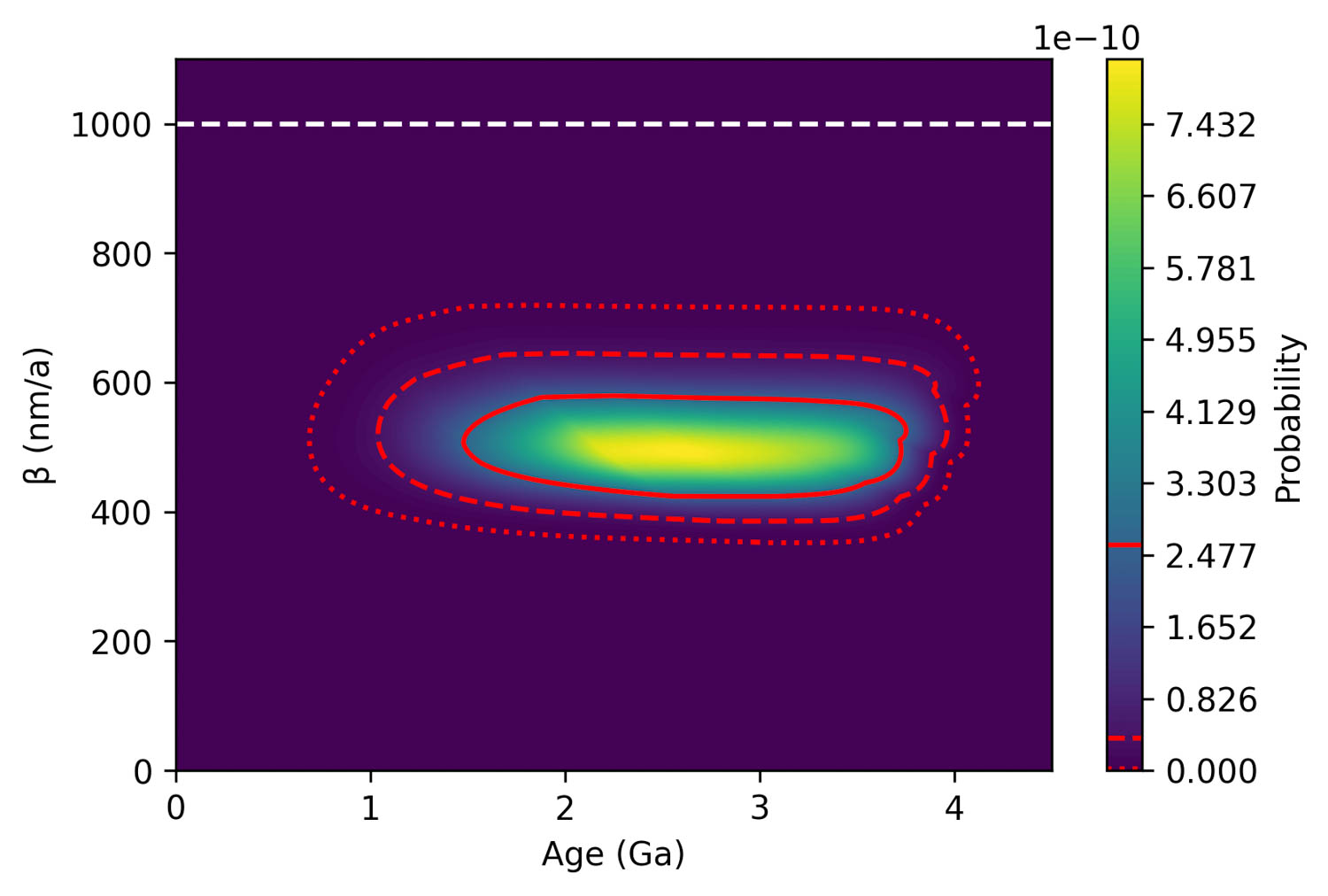
Fig. 3 Probability contour plot for site 4B Central Medusae Fossae 2B. The red solid, dashed, and dotted lines represent the 1σ, 2σ uncertainty region, and 3σ uncertainty regions. The dashed white line at 1000 nm/a indicates the minimum erosion rate needed for metastable water ice at depths shallow enough to be detected by Gamma Ray Spectroscopy (GRS) or Neutron Spectroscopy (NS). The value of 1000 nm/a is based on Figure 12 from [11].
Taking the model’s predicted best fit age and erosion rate multiplied by each site’s area, we found maximum volume and plotted a simple perspective on each site’s volume history (Fig. 4). To do this, we used the global sedimentation rate compilation of [10], who infer sedimentation rates of 10–100 µm/a for young sedimentary rocks. This is >10 times faster than our model-fit erosion rates, so we approximate sedimentation rate as instantaneous and treat deposition as one continuous interval before erosion occurs in a following continuous interval to reach present-day volume for each site.
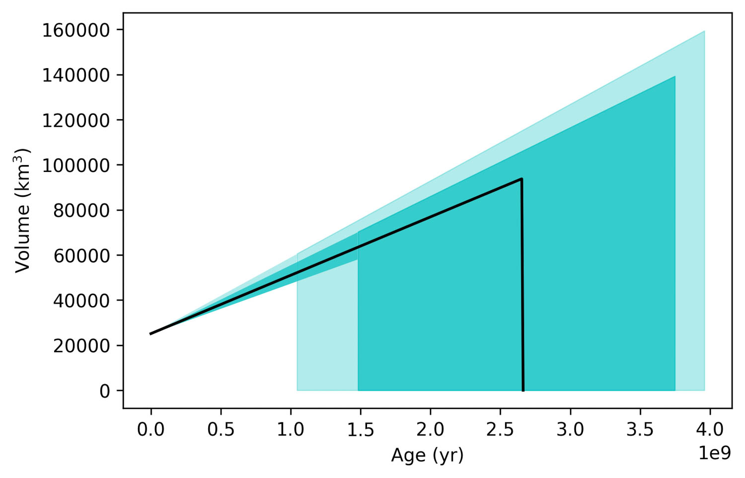
Fig. 4 Mound volume history for site 4B: Central Medusae Fossae 2B. The black line in each plot represents the cumulative best fit volume (km3) for each region. The lighter colored cyan section represents the 2σ region and the darker cyan section represents the 1σ region.
Discussion and Conclusions:
As seen in Fig. 5, while Central Medusae Fossae and Upper Mt. Sharp had best fit older ages (>1.40 Ga) and best fit lower erosion rates (<650 nm/a), East Medusae Fossae, Far East Medusae Fossae, Aeolis Planum, and Eastern Candor all had younger ages (<0.740 Ga) and higher erosion rates (>740 nm/a).
The regions with less well-defined β fits (with wider error regions) were Aeolis Planum, Eastern Candor, Far East Medusae Fossae A and C, and East Medusae Fossae B. However, four out of five of these regions had β error regions predominantly above 1000 nm/a (excluding Eastern Candor) and thus have the highest likelihood for water ice detection by GRS/NS. As a result, we recommend further investigation of these four sites due to their potential implications for in-situ resource utilization (ISRU).
Our two-parameter model using crater counts offers a more detailed understanding of sedimentary Martian surfaces with both age and β estimates compared to prior models. While the model estimates age and β values consistent with previous studies, the model estimated a much more precise β than age. Future work should focus on methods for better constraining age. As the Curiosity rover approaches Upper Mount Sharp, we will also have an opportunity to better evaluate our age and erosion rate estimations.
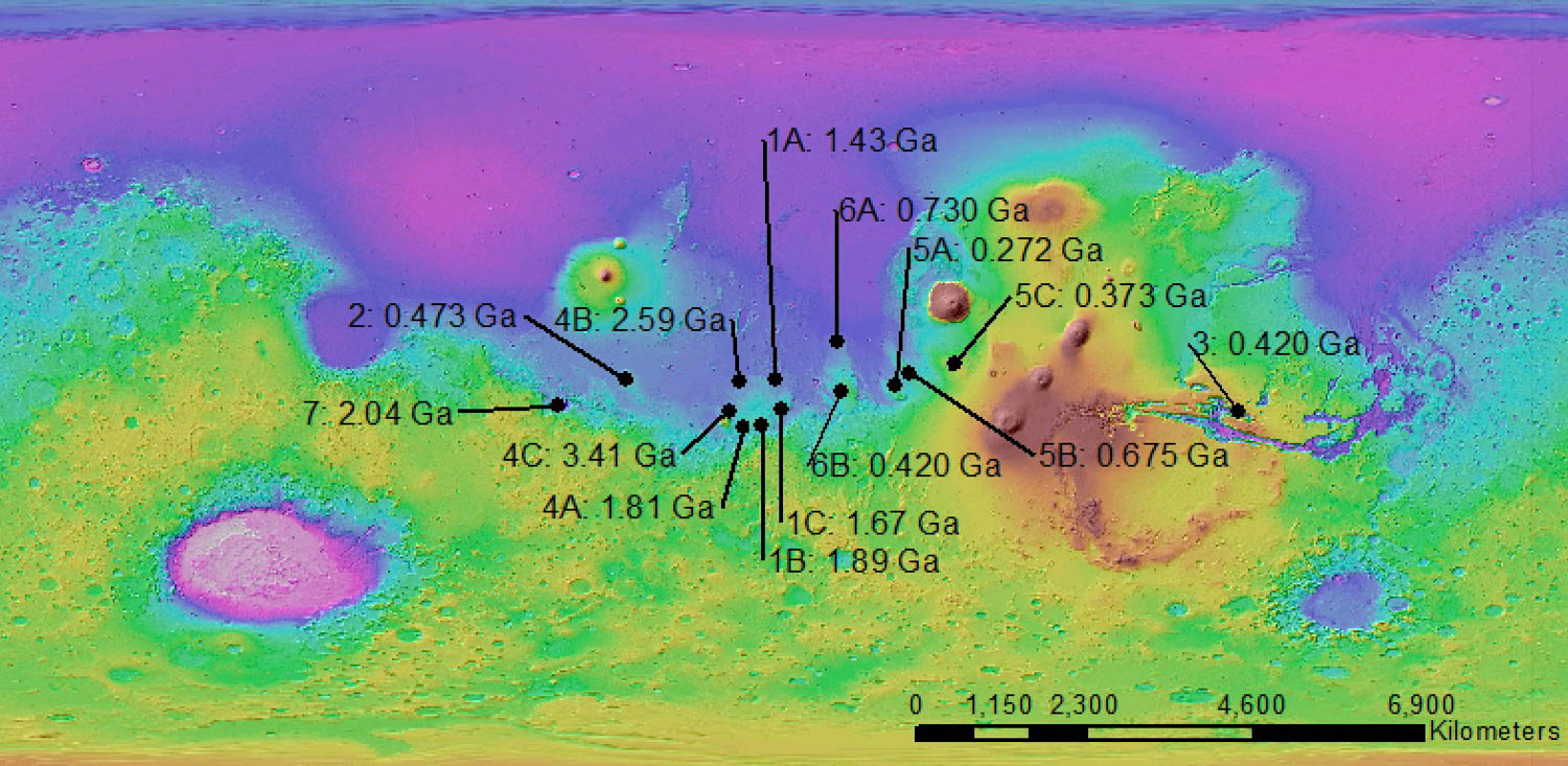
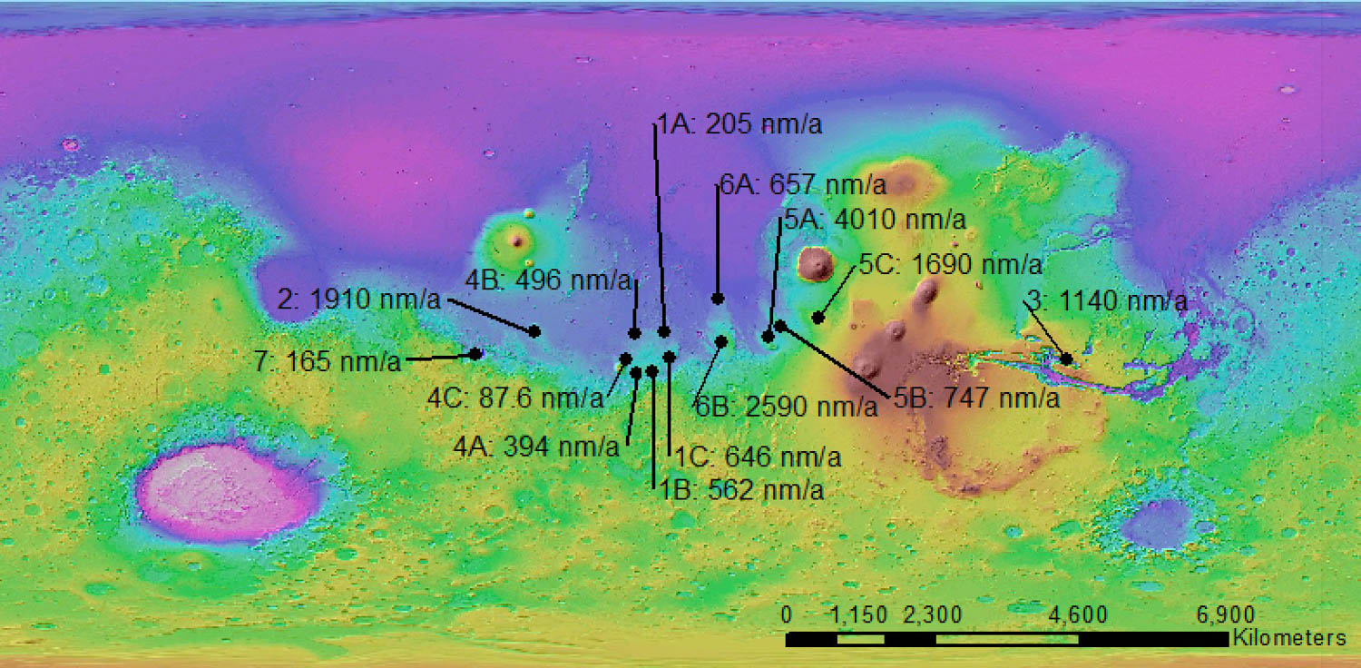
Fig. 5. Global maps of Mars with 14 study sites labeled with the model's best fit ages and β values.
Acknowledgments: We thank Katarina Keating for crater count data, as well as Daniel Fabrycky and Michael Foote for discussions.
References: [1] Kerber & Head 2010 Icarus. [2] Kerber et al. 2011 Icarus. [3] Tanaka et al. 2000 Icarus. [4] Kite and Mayer 2017 Icarus. [5] Tanaka et al. 2014 USGS SI Map 3292. [6] Orosei et al. 2017 JGR: Planets. [7] Michael 2013 Icarus. [8] Palucis et al. 2020 Icarus. [9] [10] Lewis and Aharonson 2014 JGR: Planets. [11] Hudson et al. 2007 JGR: Planets.
How to cite: Li, A. and Kite, E.: A New Probabilistic Model to Evaluate the Age and Erosion Rate of Young Sedimentary Rock on Mars, Europlanet Science Congress 2021, online, 13–24 Sep 2021, EPSC2021-462, https://doi.org/10.5194/epsc2021-462, 2021.
Gale crater on Mars records a large section of sedimentary rocks, mainly represented by the 5-km-thick sequence of Mount Sharp (Aeolis Mons). The lower part of this sequence has been explored by the Curiosity rover of the Mars Science Laboratory (MSL) mission, revealing lacustrine to fluvial depositional sequences [e.g., 1] bearing clay minerals [2]. Orbital observations highlighted the presence of clay minerals at the base of Mt Sharp but also hint at a major wet to dry environmental change with clay-bearing rocks giving way to several hundred of meters of sulfate-bearing strata [3, 4]. Orbital data coupled with rover-based observations revealed that the sulfate-bearing unit record coincides with a major change of depositional environment followed by alternation of wetter and drier conditions rather than a monotonous aridification during the Hesperian epoch [5].
Before Curiosity reached this part of Gale crater, those observations were supported using long-distance imaging capabilities of the Remote Micro-Imager (RMI) sub-system of the ChemCam instrument [6]. With a focal length of 700 mm, the RMI telescope complements the color Mastcam imagers with higher spatial resolution views of sedimentary structures and textures of rocks outcropping several hundred meters up to a few kilometers away from the rover (a ~60 km-record observation having recently been achieved, [7]). This capacity is therefore used by the MSL team both to plan future guidance of the rover and to observe geologic features from a distance. These long-distance observations pointed at the sulfate-bearing unit reveal the presence of sub-metric-scale cross-stratifications and deflation surfaces as well as diagenetic features (e.g., “satin spar”; Fig. 1). While their size allows for long-range remote observation (i.e., several hundred meters away using imagers onboard the rover, Mastcam and RMI), the resulting images lacks depth due to the distance. Yet, such 3D information can be critical in characterizing and understanding the sedimentary processes behind the setting of these structures.
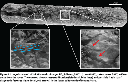
To improve our observations, we are conducting an imaging experiment to reconstruct the 3D shape of the sulfate-bearing unit outcrops with Structure-from-Motion photogrammetry using ChemCam’s RMI frames. This method is usually performed on close-range geologic features observed with other imagers onboard the rover (MAHLI, Mastcam, Navcam, [8]), but such an approach had never been applied to long-distance RMI frames. Here, we apply photogrammetric treatment to specific sets of repeated long-distance observations on the sulfate-bearing unit. To cope with the high distance of the target, we use a several-hundred meters “virtual baseline” represented by successive positions of the rover along its traverse. Figure 1 shows one of the two long-distance (1x12) RMI mosaics (ccam04947, taken on Sol 2947, cf. Fig. 2) which served as input in the stereoscopic test. This mosaic illustrates an outcrop of the sulfate-bearing unit situated ~650 meters away from the rover at that time (Fig. 2). A second similar mosaic pointed at the same target was taken on Sol 2962 (2x16 RMI mosaic, ccam04962) after the rover drove about 200 meters southeastwards (Fig. 2).
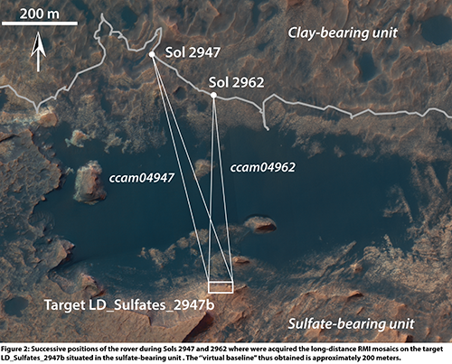
By combining the individual frames of these two mosaics in the photogrammetric chain, we were able to reconstruct the shape of the outcrop. The resulting 3D model presented in Figure 3 reveals the actual 3D shape of the imaged outcrop situated several hundred meters away from the rover, as well as displaying with improved accuracy the spatial distribution of the sedimentary and/or diagenetic structures. The use of this technique to produce long-distance 3D models will have critical implication in helping to assess and to characterize the depositional conditions related to the sulfate-bearing unit, a key objective of the Curiosity rover. The use of these models could also serve to help planning the upcoming exploration of this interval by designating high-interest targets. We also look forward to applying this method to long-distance color images obtained with the more advanced color RMI subsystem of the SuperCam instrument onboard the Perseverance rover currently operating in Jezero crater [9, 10].
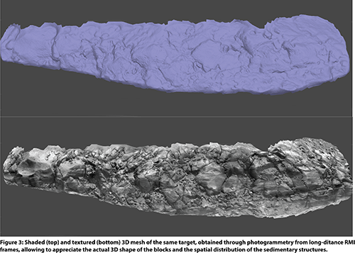
References:
[1] Caravaca et al., 2021 LSPC, abstract #1455; [2] Thorpe M. T. et al., 2021, LPSC, Abstract #1519; [3] Miliken et al., 2010, Geophys. Res. Lett. 37, L04201; [4] Fraeman A. A. et al., 2016, J. Geophys. Res. Planets 121, 1713–1736; [5] Rapin et al., 2021, Geology 49; [6] Le Mouélic et al., 2015, Icarus 249, 93-107; [7] Le Mouélic et al., 2021, LPSC Abstract #1408; [8] Caravaca et al., 2020, Planet. Space Science 182, 104808; [9] Gasnault et al., 2021, LPSC Abstract #2248; [10] Gasnault et al., 2021, EGU Abstract #EGU21-16461.
How to cite: Caravaca, G., Le Mouélic, S., Rapin, W., Dromart, G., Fau, A., Mangold, N., Le Deit, L., Gasnault, O., Wiens, R. C., and Lanza, N. L.: Reconstructing the 3D shape of sulfate unit outcrops (Gale crater, Mars) using ChemCam’s Remote Micro Imager onboard the Curiosity rover., Europlanet Science Congress 2021, online, 13–24 Sep 2021, EPSC2021-164, https://doi.org/10.5194/epsc2021-164, 2021.
1. Introduction
The north polar region of Mars is one of the most active places of the planet with avalanches[1] and ice block falls[2] being observed every year on High Resolution Imaging Science Experiment (HiRISE) data. Both phenomena originate at the steep icy scarps surrounding the north polar plateau, Planum Boreum. The exposed layers of ice and dust contain important information about the climate cycles of the planet[3]. We are interested in monitoring how the current scarp erosion rate (quantified through analysing block falls) is linked to these periodic changes in temperature. The large scale of the region of interest, combined with a growing amount of available satellite data makes automation key for this project. Our goal is to monitor robustly the whole north polar region for ice block falls throughout the entire Mars Reconnaissance Orbiter (MRO) mission. The active scarps of the north polar region contain two main geological units, the older and darker Planum Boreum Cavi unit, also called Basal Unit (BU) and the younger and brighter Planum Boreum 1 unit, which is a part of the so called North Polar Layered Deposits (NPLD)[4]. These geologic units are mapped by Tanaka et al. (2012), however the scale of this map is not sufficient for our work, as it is based on coarse resolution data. For our project it is important to segment the HiRISE images of the steep scarps in NPLD and BU regions with high precision, both to restrict the area where the algorithm will look for fallen blocks and to differentiate between the activity originating in the NPLD[5] from that originating in the BU. Here we present our algorithm for automated scarp mapping – the first completed step towards a fully streamlined monitoring pipeline.
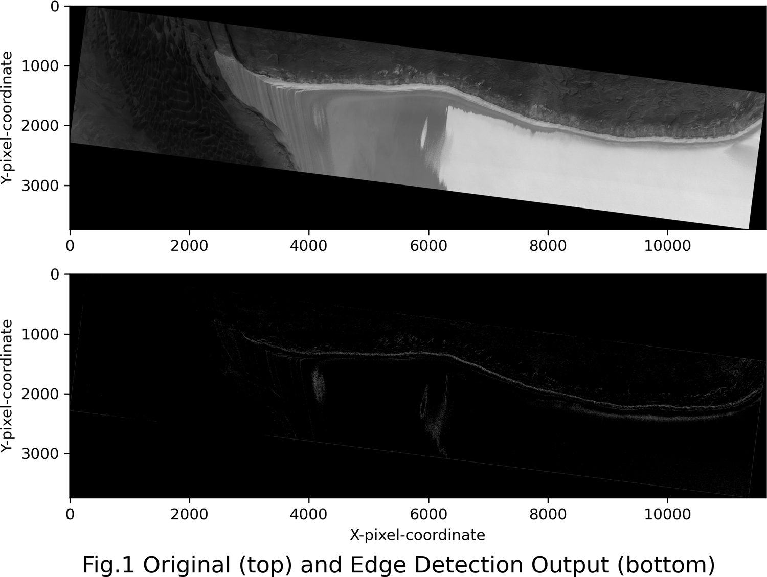
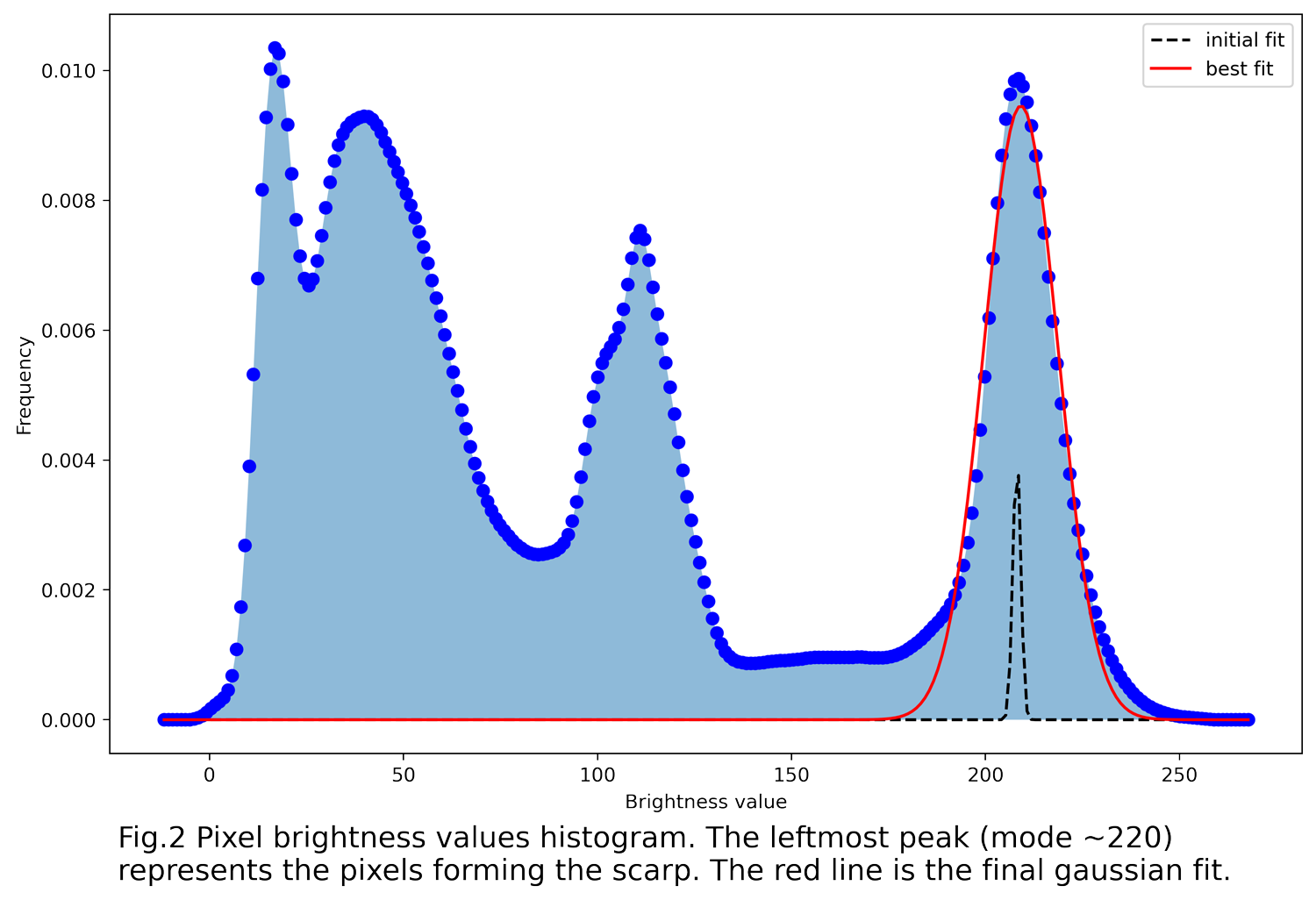
2. Methods and Results
First the original high-resolution images have to be downscaled by 90% in both dimensions. Given the initial 0.3 m/pixel precision, this procedure increases the delineation error margin to about 3 meters. This tradeoff is required to achieve greater computational efficiency during the subsequent pre-processing steps. OpenCV canny edge detection (CED) algorithm can then be applied to the downscaled result, yielding a binary contour map (Fig.1). Two parameters have to be specified when running edge detection, namely: min and max thresholding values. These are used by the algorithm to decide whether an edge is to be kept or to be discarded. We propose a fully automated method for choosing the optimal constraints. Our approach relies on the fact that the exposed scarp produces a spike in the histogram of pixel brightness values. We utilize kernel density estimation (KDE) to fit a gaussian distribution to this area of the histogram and then select its 5th percentile and mode as minVal and maxVal respectively (Fig.2). The CED output contains both the scarp trace and the noise resulting from numerous other objects present in the FOV (Fig.3 bottom left). To filter out the unnecessary detail, we roll a sliding window across the image, tracking areas containing many pixels with high edge responses. The y-coordinate of every new box in a sequence is adjusted to follow the underlying bright pixels as tightly as possible. The longest of the sequences is expected to contain the scarp and therefore only its content is retrieved (Fig.3 top). Since CED struggles to connect all the separate edges at such a large scale, the boundary of the scarp is delineated by a collection of disjointed lines (Fig.3 bottom left). Before we can derive a continuous polynomial that can bridge the gaps in between these lines, an even more rigorous de-noising is required. We propose a two-stage procedure based on density clustering[6]. The whole length of the scarp is first divided into overlapping segments. HDBCSAN is then applied to each segment independently, yielding numerous clusters of varying size (Fig.3 bottom right). We proceed by linking these clusters through sets of shared points located in the overlap areas. As a result, the scarp trace is represented by the largest grouping of pixel co-ordinates and all the smaller clusters are discarded. Upon tightening the parameters of HDBSCAN to filter out the finer noise ignored by the previous crude sweep, we obtain the final scarp outline. This preprocessed contour map is then subjected to a custom data boundary fitting algorithm, which uses cubic splines to connect the adjacent edges[7] (Fig.4). Since the resolution, sliding window sizes and scarp segmentation schemes are kept constant between the images, most of the internal parameters can be set to sensible defaults, thus minimizing the user input.
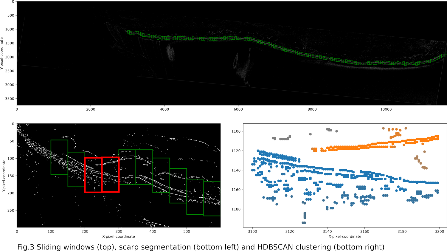
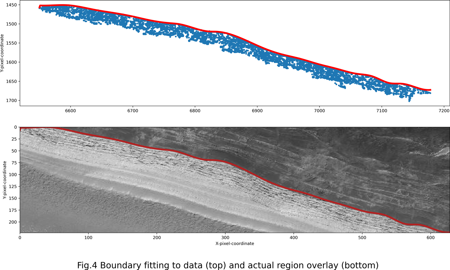
3. Conclusions and future projects
Our first step towards fully monitoring the activity of the north polar region resulted in a detailed and automatically produced map of the boundary between BU and the NPLD based on the significant difference in intensity between them. Fanara et al. (2020a) already used traditional machine learning techniques to detect newly appeared ice blocks, achieving a good performance and estimating the current erosion rate of a steep scarp[8]. We are now planning to complement this study with our scarp mapping algorithm. This should allow to further extend the training dataset, hopefully generating enough input for a computer vision model based on convolutional neural networks. The NPLD remains our primary area of interest due to its high levels of activity and good image density, yet we also plan to apply our pipeline to different surface changes and Martian regions as well as other celestial objects.
References
1. Russell P., Thomas, N. Byrne, S. Herkenhoff, K. Fishbaugh, K. Bridges, N. Okubo, C. Milazzo, M. Daubar, I. Hansen. Seasonally active frost-dust avalanches on a north polar scarp of Mars captured by HiRISE, Geophys. Res. Lett. 35, L23204, 2008.
2. L. Fanara, K. Gwinner, E. Hauber, J. Oberst. Present-day erosion rate of north polar scarps on Mars due to active mass wasting, Icarus, Volume 342, 2020,113434, ISSN 0019-1035.
3. Smith I.B., Putzig N.E., Holt J.W. and Phillips R.J. An ice age recorded in the polar deposits of Mars, Science, 352, 1075–1078, 2016.
4. Tanaka, K.L., and Fortezzo, C.M., 2012, Geologic map of the north polar region of Mars: U.S. Geological Survey Scientific Investigations Map 3177, pamphlet 11 p., 1 sheet, scale 1:2,000,000.
5. Su, S., Fanara, L., Zhang, X., Gwinner, K., Hauber, E., and Oberst, J.: Sources of ice block falls at the Martian north polar scarps: detection from multi-temporal HiRISE image sets, EGU General Assembly 2021, online, 19–30 Apr 2021, EGU21-7489.
6. Leland McInnes1, John Healy1, and Steve Astels2. HDBSCAN: Hierarchical density-based clustering. (1) Tutte Institute for Mathematics and Computing, (2) Shopify.
7. N. Cardiel. Data boundary fitting using a generalized least-squares method; Mon. Not. R. Astron. Soc. 396, 2009, ISSN 680–695.
8. L. Fanara, K. Gwinner, E. Hauber, J. Oberst. Automated detection of block falls in the north polar region of Mars, Planetary and Space Science, Volume 180, 2020, 104733, ISSN 0032-0633.
How to cite: Martynchuk, O., Fanara, L., Gwinner, K., Hauber, E., and Oberst, J.: Automated NPLD scarp mapping for the block falls monitoring pipeline, Europlanet Science Congress 2021, online, 13–24 Sep 2021, EPSC2021-712, https://doi.org/10.5194/epsc2021-712, 2021.
Abstract
Previously, we have proposed and validated the co-registration of local dynamic Mars Orbiter Laser Altimeter (MOLA) profile segments to static Digital Terrain Models (DTMs) as an approach for obtaining seasonal CO2 ice cover height variations on Mars. Building upon this, we introduce a post-correction procedure called “bi-RPCA” to further lower residual errors in the profiles and improve the precision of the height variation measurements. The ultimate goal is to apply this method to MOLA, SHAllow RADar (SHARAD) radar altimetry to generate long-term seasonal height change time series at the Martian poles with high spatial and temporal resolution.
1. Introduction
The dynamic growth and retreat of Martian polar CO2 ice/frost caps is one of the most important themes for the Red Planet’s climate [1, 2]. Accurate measurements of seasonal height and volume changes of snow and ice can serve as important constraints for models of Mars climate and the long-term evolution of the southern residual ice cap. Previously, we have proposed and validated the local co-registration between laser profile segments and high static resolution DTMs in obtaining the temporal height variations at local scale [3]. Building upon that, we now propose a post-correction procedure called “bi-RPCA” to further improve the precision of the obtained height variation time series.
2. Data
The Mars Orbiter Laser Altimeter (MOLA) Precision Experimental Data Record (PEDR) dataset includes a total of 8505 profiles, acquired in the mapping and extended phases of Mars Global Surveyor (MGS) from February, 1999 to May, 2001, which spanned approximately a full Martian year [1]. The PEDR dataset was processed using a MGS orbit trajectory- and a Mars rotational model by GSFC dating back to 2003. Therefore, we reprocessed the MOLA data, incorporating a refined orbit model from [4] and the IAU2015 Mars rotational model [5] for new MOLA geolocations. To account for the special relativity effect, a pointing aberration correction has also been applied in the reprocessing [6].
3. Methods
3.1. Self-registration technique
To build coherent reference DTMs of the average Martian surface at South Pole [78°S, 87°S] and an annulus centered at 50°S ([44°S, 56°S]), we resort to the self-registration of the reprocessed MOLA profiles [7, 8].
3.2. Localized co-registration
In order to obtain the height change series, the following steps are performed. First, small segments of the MOLA profiles consisting of a few hundred footprints are co-registered to the reference DTM. In this step we use a window, which is moved along the footprints. The obtained height corrections are assigned to the central footprint within the window. Hence, one obtains an individual height correction for every footprint within the MOLA profile and observation epoch. Finally, the CO2 height change time series are obtained by median-binning those temporal height differences with the precision quantified by scaled median absolute deviation. We name this method “F_LC” [3], where “F” stands for footprints and “LC” the local co-registration.
3.3. Post-correction by regional pseudo cross-over adjustment
The regional crossover adjustment (RCA) over a relatively small & non-dynamic areas has been extensively used to improve the internal consistency of biased altimetry profiles on Earth [9]. Here, we adopt the DTM-based pseudo cross-overs acquired within 5 Earth days instead of the traditional cross-overs in the process as the regional pseudo cross-over adjustment (RPCA) for post-correction purposes. Pseudo cross-overs are formed by two profile segments that do not necessarily intersect. However, the connection between the profiles is established by a DTM overlapping with both profiles. Hence, the height difference between these (not necessarily crossing) profiles is obtained by the difference of their height corrections with respect to the self-registered DTM. Due to the inclusion of these pseudo cross-overs the number of “cross-overs” is increasing significantly [10]. The height correction is assumed to be constant for each profile segment. “Bi-RPCA” consists of two consecutive RPCA processes. By performing the RCPA at 50°S annulus, where no seasonal effects are expected, we obtain corrections for a systematic temporal bias within the MOLA data [2]. By assuming that the correction for a specific profile does not change from 50°S to the polar area, we apply the same corrections for profiles at the polar regions. The second RPCA step is carried out in the polar region to obtain height corrections to improve the self-consistency of the profiles, and hence the precision of the obtained temporal height variation using "F_LC".
4. Results
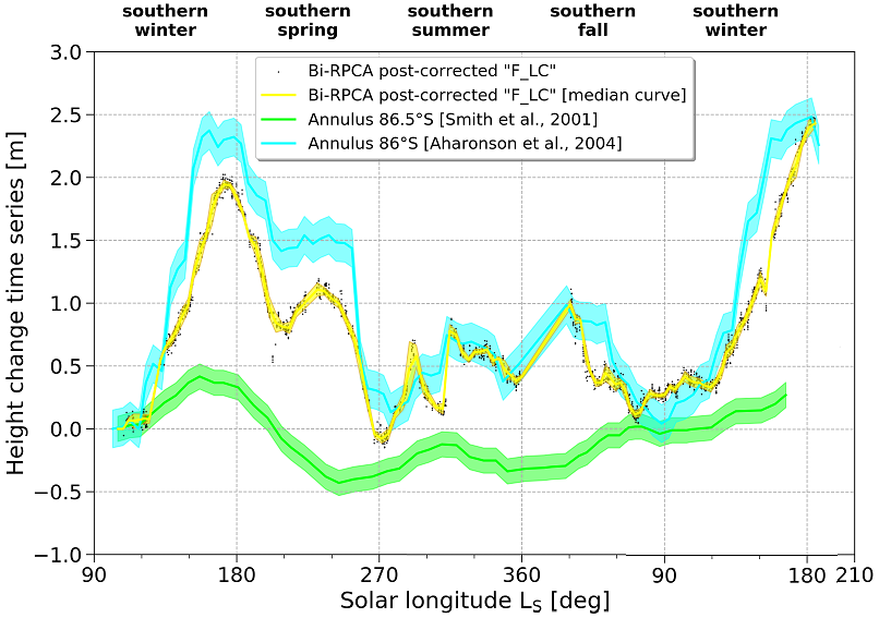
Figure 1: Temporal height variation for a polar region along 86°S ([85.75°S, 86.25°S, 270°E, 280°E]) by our “F_LC” & bi-RPCA approach in comparison with results for an annulus at 86.5°S [1] and 86°S [2].
An example of the obtained temporal height variation in study region on the residual ice cap using “F_LC” and post-corrected by “bi-RPCA” is shown in Figure 1. The peak-to-peak height variation is ~2.5 m, similar to that of [2]. However, the peak height in MY25 is ~0.5 m higher than that of MY24, indicating annual variations. The off-season accumulation in southern summer and fall resolved in [2] are clearly visible in our result. The precision quantified by scaled median absolute deviation (the yellow shade in Figure 1) is ~4 cm, much improved over the ~50 cm of the “F_LC” result without the “bi-RPCA” post-correction [3].
5. Summary
We propose the “bi-RPCA” post-correction procedure to simultaneously compensate for systematic temporal bias and remove residual errors in the reprocessed MOLA profiles. The obtained height variation time series at the study region is reaching a high precision of ~4 cm. Thus, in future work the combination of “F_LC” & “bi-RPCA” will be applied to the entire polar regions to map the spatial distribution of the varying depth of the seasonal ice caps.
Acknowledgements
H. Xiao thanks China Scholarship Council (CSC) for financial support of his study in Germany. Part of this research was carried out within the framework of the DLR BigData Querschnittsplattform.We acknowledge the work by the MOLA instrument and science teams.
References
[1] Smith et al., Science, 2001, 294, 2141-2146. [2] Aharonson et al., JGR Planets, 2004, 109(E5). [3] Xiao et al., EPSC2020, vol.14, No. 181. [4] Konopliv et al., Icarus, 2006, 182, 23-50. [5] Konopliv et al., Icarus, 2016, 274, 253-260. [6] Xiao et al., JoG, 2021, 95(2), 1-23. [7] Stark et al., EPSC2018, Contrib. No. 890. [8] Stark et al., GRL, 2015, 429, 7881-7889. [9] Ewert et al., J. Geodyn., 2012, 59-60, 111-123 [10] Barker et al., Icarus, 2016, 273, 346-355.
How to cite: Xiao, H., Stark, A., Steinbrügge, G., Thor, R., Schmidt, F., and Oberst, J.: Mapping height variations of seasonal ice cover at the Martian South Pole, Europlanet Science Congress 2021, online, 13–24 Sep 2021, EPSC2021-428, https://doi.org/10.5194/epsc2021-428, 2021.
Introduction: Recurring Slope Lineae (RSL) are narrow dark streaks that incrementally lengthen down Martian warm steep slopes [1]. On first approximation, they appear during the Martian summer, disappear in winter and recur annually. This temperature dependence suggested that RSL may be related to flows of liquid water or brines [1-5], possibly fed by groundwater sources [6, 7] or from the deliquescence of hygroscopic salts [8]. Alternatively, RSL have been interpreted as dry granular flows [9, 10, 11, 12], possibly related to aeolian processes [13, 14]. Although a detailed explanation of the RSL nature and formation mechanism is still not complete, the latest evidence points further toward a dry mechanism [15].
Here, we provide further evidence for a dry origin of RSL by investigating their colour properties through multiband photometry obtained from 4-filter Colour and Surface Science Imaging System (CaSSIS, [16]) observations at Horowitz crater, Mars. We compare it with multiband photometry of dark tracks left by the passage dust-devils (DDTs), which are dark marks left by the passage of whirlwinds, and regions where surface dust has been partially removed (“dust poor” regions, DPs). Since DDTs and DPs are being formed by ferric dust removal and the exposure of underlying, typically ferrous material, the comparative multiband photometry provided by CaSSIS may help us understand whether RSL are consistent with being formed by the removal of dust. This would contribute to show that RSLs are indeed dry flows of dust and sand. Our comparative photometry is then supported by a photometric modeling approach.
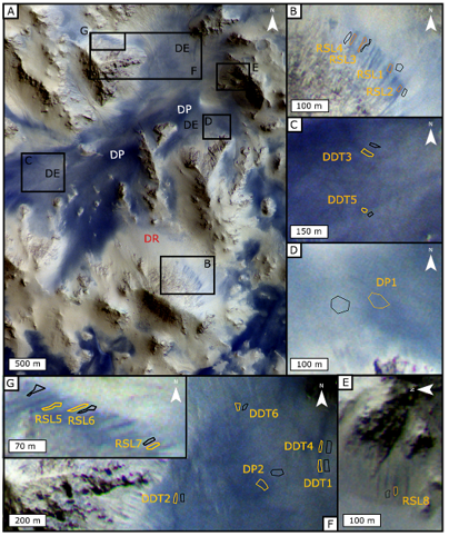
Figure 1 CaSSIS NPB (i.e., NIR PAN, BLU) colour composite showing the central peak of Horowitz crater and the location of the RSL, DDTs and “dust-poor” (DP) ROIs. “DR” indicate dust rich regions, “DE” indicate “dust-enriched” regions (i.e., with an intermediate dust content between DP and DR)
Methodology: We adapted the technique of [11,12] to compute the relative reflectance of RSL in the NIR (936.7 nm), RED (836.2 nm), PAN (675.0 nm) and BLU (499.9 nm) BLU CaSSIS filters. To do this, we select several regions of interest (ROIs) within RSLs, DDTs and DPs at Horowitz crater. The considered ROIs are shown in Fig. 1. We compute for each filter the RSL relative reflectance as in [11,12] and we repeat the procedure for DDTs and DPs. In our calculations, we apply a first order atmospheric correction by subtracting the I/F of the darkest pixel of each filter before computing the relative reflectance [16,17,18]. The relative albedo profiles are then compared with photometric models of dust deposition derived from the laboratory experiments of [19] and with mixtures of wet and dry martian terrain simulants derived from [20].

Figure 2. Relative albedo of A) RSL B) DDTs and C) DP ROIs with respect to nearby materials and D) corresponding average profile
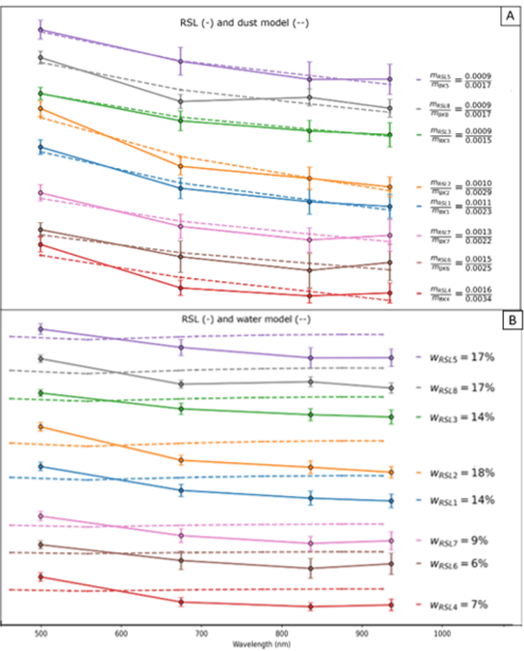
Figure 3. A) RSL and best-fit dust models. The legend reports the estimated dust content for the RSL (numerator) and corresponding nearby material (denominator). B) RSL and best-fit water models. The legend reports the best-fit water content
Results: RSL, DDTs and DPs have similar relative reflectance profiles (Figure 2) within errors, i.e., they are all brighter in the BLU than in the PAN, RED and NIR filters. While there is some variability, there are no significant spectral features that characterize either RSL or DDTs or DPs in the latter three bands, where all show an approximately constant relative reflectance. In addition, photometric models of dust fallout provide significantly better fits than mixtures of dry and wet martian terrain simulants.
Discussion and conclusions: The comparison between relative photometry of RSLs, DDTs and DPs in the 4 CaSSIS filters show that these features have a quite similar relative reflectance profile, suggesting that they may have a similar origin. In particular, the higher BLU with respect to PAN, RED and NIR relative reflectance may suggest that the reflectance profiles of both features could be consistent with a ratio between a ferrous material (numerator), exposed by the removal of a ferric surface material such as the Martian dust (denominator). This picture is supported by comparison with photometric model of dust fallout, that consistently provide better fits to the observed relative reflectances than mixtures of dry and wet martian soils.
Acknowledgments: The authors wish to thank the spacecraft and instrument engineering teams for the successful completion of the instrument. CaSSIS is a project of the University of Bern and funded through the Swiss Space Office via ESA’s PRODEX programme. The instrument hardware development was also supported by the Italian Space Agency (ASI) (ASI – INAF agreement no. I/018/12/0), INAF/Astronomical Observatory of Padova, and the Space Research Center (CBK) in Warsaw. Support from SGF (Budapest), the University of Arizona (Lunar and Planetary Lab.) and NASA are also gratefully acknowledged. The study has been supported by the Italian Space Agency (ASI-INAF agreement no. 2020-17-HH.0).
References: [1] A. S. McEwen et al. (2011), Science (6043), 740–743 [2] Levy, J et al. (2012), Icarus, 219, (1), 1-4 [3] McEwen et al. (2014), Nat. Geosci. 7 (1), 53–58 [4] Stillman et al. (2014), Icarus 233, 328–341 [5] Huber et al., (2020) Icarus 335, 113385. [6] Stilllman et al. (2016), Icarus 265, 125–138. [7] Abotalib and Heggy (2019) ,Nat. Geosci. 12, 235–241 [8] Wang et al. (2020), Icarus 333, 464–480 [9] Dundas et al. (2017), Nat. Geosci. 10 (12), 903–907 [10] Schmidt et al. (2017), Nat. Geosci. 10 (4), 270–273 [11] Schaefer et al. (2019), Icarus 317, 621–648 [12] Munaretto et al. (2020), PSS 187, (2020), 104947 [13] Vincendon et al. (2019), Icarus 325, 115–127 [14] Dundas et al. (2020), Icarus 343, 2020, 113681 [15] McEwen, A. S. et al. (2021), JGR-Planets, in press. [16] Thomas et al. (2017) Space Sci. Rev. 212 (3–4), 1897–1944[17] Chavez Jr, P. S. (1988) .Remote sensing of environment, 24(3), 459-479. [18] Tornabene et al. 2018, SSR,214(1),18 [19] Wells et al., 1984, Icarus 58, 3, 331-338 [20] Gunderson et al 2007, PSS, 55, 10, 1272-1282
How to cite: Munaretto, G., Pajola, M., Lucchetti, A., Cremonese, G., Simioni, E., Re, C., Bertoli, S., Tornabene, L., McEwen, A. S., Becerra, P., Rangarajan, V. G., Valantinas, A., Pommerol, A., Thomas, N., and Portyankina, G.: Multiband photometry of Martian Recurring Slope Lineae (RSL) and dust-removed features at Horowitz crater, Mars from TGO/CaSSIS color observations, Europlanet Science Congress 2021, online, 13–24 Sep 2021, EPSC2021-379, https://doi.org/10.5194/epsc2021-379, 2021.
Introduction: Martian meteorites are the only samples from the Red Planet available for in-depth laboratory analyses. More than 280 pieces of 152 unique samples, originating from at least 11 source craters, are curated in the world’s collections [1]. Ejection ages, based on cosmic ray exposure (CRE), vary from 0.7 to 20 Myr [2-4]. The ejection sites are still unknown, despite several previous propositions [5-7], motivated by the significance of establishing a link between the crystallization ages, and the chemical and mineralogical properties of these samples with surface geology.
Secondary impact craters, the key to identify the meteorites ejection sites: The formation of an impact crater generates debris ejected with speeds above and below the escape velocity on Mars (5 km/s). The fraction of ejecta material with a velocity higher than the escape velocity may get through the Martian atmosphere and into the interplanetary space. Numerical simulations suggest that impact events capable of producing such fragments would form craters larger than ~3 km in diameter on the Martian surface [8-9]. Material with a velocity lower than 5 km/s falls back to the surface in a radial pattern or rays around the primary source crater and forms secondary craters with a maximum size of about 2 to 5% of the primary crater diameter [10-12]. These secondaries are shallower than those formed by primary impacts and are rapidly eroded. Typically, a secondary crater of 100 m in diameter would be completely erased in about 50 Myr. Therefore, the occurrence of radial patterns of small secondaries is a diagnostic feature of young primary craters [6,13-14]. The use of high-resolution imagery would allow the identification of such small craters, but manual mapping of the tens of millions of secondary impact craters constellating the surface of Mars is not feasible.
Machine learning approach to identify small craters on high-resolution images: We adapted an automated Crater Detection Algorithm (CDA) [15] to identify craters smaller than 1 km in diameter across the entire surface of Mars. The algorithm was trained using High-Resolution Imagery System Experiment (HiRISE) images (25 cm/pixel) and applied on the global Context Camera (CTX) mosaic [16] (6 m/pixel), thus generating a database of more than 90 million detections (Figure 1).

Figure 1: Crater Size-Frequency Distribution of the automatic crater database (in red) compared to the manual catalogue (in blue) from [11-12].
We evaluated the performance of our model against ~1000 impact craters >60 m (10 pixels in diameter on CTX imagery) manually mapped on 6 different geological units, thus constituting the ground truth (GT). For craters > 100 m in diameter, it results in an average true positive detection rate (or recall) of more than 80% and an average precision of 96%. The diameter estimation derived from our model is within 25% of uncertainty compared to our ground truth (Figure 2), which is within the expected human performance [17].

Figure 2: Comparison between the difference in the diameter of craters estimated by the CDA and the ground truth (black crosses). The kernel density estimator shows that detections larger than 100m are estimated within 25% of uncertainties compared to manually identified impact craters.
The ejection site of a group of Martian meteorites: We analyzed the spatial and size distribution of craters smaller than 300 m by computing a crater density map from this dataset. The figure 3 presents the results obtained by combining three density maps with red, green, and blue channels corresponding to local crater density (in a 0.05° grid) for three diameter size ranges, in order of decreasing range of diameter, respectively 150 < D < 300 m, 75 < D < 150 m and < 75 m. Using this map, we identified 19 secondary ray systems associated with large and recent primary craters (Figure 3).

Figure 3: Density map of craters < 300 m in diameter (89,054,458 entries). Colors indicate crater densities of specific diameter ranges (see text for details).
Using crater counts on the ejecta blanket of each of those 19 impact craters and their surrounding terrains, we derived respectively the model age of those impacts and the age of the impacted material. Those results are compared with the ejection age of Martian meteorites as well as their crystallization ages. We found that two craters, both located in the Tharsis volcanic province, are the most likely source of depleted Shergottites launched ~1 Myr ago [3]. Considering the magmatic ages and the petrogenesis of these samples, this implies that a major thermal anomaly deeply rooted in the mantle under Tharsis was active over most of the geological history of the planet, and has sampled a depleted mantle that has retained geochemical signatures of Mars’ early history.
References: [1] https://www.lpi.usra.edu/meteor/metbull.php. [2] Herzog, G.F., & Caffee, M.W. Treatise on Geochemistry, 1, 419-454 (2014). [3] Lapen, T.J., et al. Sci. Adv., 3(2), e1600922 (2017). [4] Udry, A., et al. J. Geophys. Res., 25, e2020JE006523 (2020). [5] Werner, S. C., et al., Science, 343, 1343–1346 (2014). [6] McEwen, A.S., et al. Icarus, 176, pp. 351-381 (2005). [7] Mouginis-Mark, P.J. & Boyce, J.M. Chemie der Erde - Geochemistry, 72, 1-23 (2012). [8] Artemieva, N., & Ivanov, B.A. Icarus, 1, 84-101 (2004). [9] Head, J.N., et al., Science, 298, 1752-1756 (2002). [10] Lagain, A., et al., in Reimold, W.U., and Koeberl, C., eds., Large Meteorite Impacts and Planetary Evolution VI, 550, p. 1-16 (2021). [11] Robbins, S.J., & Hynek, B.M. J. Geophys. Res., 117, E05004, (2012). [12] Robbins, S.J. & Hynek, B.M. J. Geophys. Res., 116, E10003 (2011). [13] Hartmann, W.K., et al., Icarus, 208, 621-635 (2010). [14] Tornabene, L.L., et al. J. Geophys. Res., 111, 1-25 (2006). [15] Benedix, G.K., et al. Earth. Sp. Sci., 7, e2019EA001005 (2020). [16] Dickson, J.L., et al., 49th Lunar and Plan. Sci. Conf. (2019). [17] Robbins, S.J., et al. Icarus, 234, 109–131 (2014).
How to cite: Lagain, A., Benedix, G., Servis, K., Baratoux, D., Doucet, L.-S., Rajšic, A., Devillepoix, H., Bland, P., Towner, M., Sansom, E., and Miljković, K.: Counting 90 million craters on Mars to find the source of meteorites, Europlanet Science Congress 2021, online, 13–24 Sep 2021, EPSC2021-12, https://doi.org/10.5194/epsc2021-12, 2021.
Over 20% of organic carbon in sediments on Earth are bound to reactive Fe mineral phases [1]. These reactive Fe phases are generally Fe (oxyhydr)oxides, often associated with clay minerals. It is important to note that they occur as nanoparticulate and X-ray amorphous phases that are challenging to identify. On Earth, proxy methods such as chemical sequential extractions are often used but they can produce misleading results when used for mineral identification [2,3]. We develop and use Mössbauer spectroscopy applications to identify these phase [2-4] and compare these to Raman spectroscopy because the Mars 2020 Perseverance rover and the ExoMars 2022 Rosalind Franklin rover use Raman spectrometers for mineralogical identification.
Reactive Fe phases are abundant on Mars. It is important to note that they are not the well-crystalline expression of Fe (oxyhydr)oxides such as hematite and goethite that have been observed from orbit and with a variety of rover-based instruments. Instead, reactive Fe phases are represented by as yet unidentified Fe phases: Aqueously altered rocks and soils in Gusev crater and at Meridiani Planum (including the Burns formation) contain large amounts of nanophase iron oxides (npOx and Fe3D3) [5]; and 20-60 wt% of minerals in fluvio-lacustrine deposits in Gale crater are X-ray amorphous and this amorphous phase is rich in iron [6]. Mineralogical interpretation of CRISM data of Rosalind Franklin's landing site at Oxia Planum also suggest the presence of these phase. These reactive Fe phases can be any combination of a number of minerals including ferrihydrite, lepidocrocite, akaganèite, hissingerite, schwertmannite, and superparamagnetic (i.e. nanoparticulate) hematite and goethite [5].
The preservation of organic compounds by reactive Fe species is effective over hundreds of thousands of years in Earth sediments [1]. In return, organic compounds slow down the transformation of reactive Fe species such as ferrihydrite into the more crystalline and thermodynamically stable Fe (oxyhydr)oxides hematite or goethite during diagenetic processes. With temperature and pressure rising further during diagenesis, however, organic compounds are oxidized and destroyed through the reduction of Fe (resulting in the diagenetic formation of the Fe carbonate siderite, for example), and the non-reduced Fe species are transformed into thermodynamically stable minerals. Thus, the presence of reactive Fe species in Martian sediments/sedimentary rocks indicates only little diagenetic overprinting and therefore a high preservation potential of organic compounds. Such samples will be of high priority for analysis with MOMA. However, the presence of Fe species during pyrolysis can reduce the detectability of certain organic compounds. This effect depends on the specific Fe species present and is mitigated in the presence of clay minerals [7,8].
We will present Mössbauer and Raman spectrocopy investigations of reactive Fe phases in various sedimenatry settings and compare these results into the context of rover landing sites on Mars.
References:
[1] Lalonde et al (2012) Nature 483, 198-200. [2] Schröder et al (2016) Hyperfine Interact 237, 85. [3] Hebpburn et al (2020) Chem Geol 543, 119584. [4] Klingelhöfer et al (2003) J Geophys Res 108(E12), 8067. [5] Morris et al (2019) in Remote Compositional Analysis: Techniques for Understanding Spectroscopy, Mineralogy, and Geochemistry of Planetary Surfaces, pp. 538-554, Cambridge University Press. [6] Rampe et al (2017) Earth Planet Sci Lett 471, 172–185. [7] Tan et al (2021) Astrobiology 21, 199-218. [8] Royle et al (2021) Astrobiology in press.
How to cite: Schröder, C. and Bonsall, E.: Preservation of organic compounds and constraints on diagenetic processes by reactive iron phases on Mars, Europlanet Science Congress 2021, online, 13–24 Sep 2021, EPSC2021-771, https://doi.org/10.5194/epsc2021-771, 2021.
Introduction: The Mars Odyssey (MO) mission is the longest-lasting spacecraft on Mars. Launched in 2001, the orbiter has provided an unprecedented temporal coverage ranging from Martian Year (MY) 25 (Feb 2002) to current MY 36 [1]. The Neutron Spectrometer (NS) is one of the instruments onboard MO, and it has been surveying the shallow (~first meter) subsurface of Mars for hydrogen to map its amount and global distribution [2]. MO/NS measurements have been used to locate the main reservoirs of hydrogen content on Mars (Fig. 1) [3].
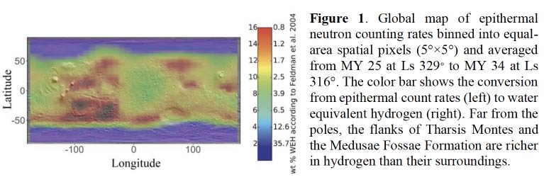
The flux of neutrons leaking from Mars’ surface is inversely related to the hydrogen content of the soil. This is because hydrogen is especially effective at moderating neutrons generated through collisions between cosmic rays and atoms in the Martian soil. Based on this principle, MO/NS collects neutron fluxes in three consecutive energy bands: thermal (0-0.3 eV), epithermal (0.3 eV-700 keV) (ECR), and fast (0.7-5 MeV) neutron ranges. Among these, epithermal neutrons are more useful in interpreting hydrogen abundance, as they are less sensitive to variations in the soil’s amount of heavy elements.
MO/NS measurements are sensitive to the hydrogen content of the soil, but not to the type of molecular association of such hydrogen. Potential hydrogen carriers in the Martian soil include: (1) buried water ice, (2) structural water bound in salts (chemisorbed water), and (3) water molecules adsorbed on the surface of soil grains and minerals (physisorbed water) [4]. Potential shallow subsurface water ice reservoirs far from the poles are of special interest, because they may constitute an important source for future In-Situ-Resource-Utilization (ISRU).
Objective: Here, we look for shallow subsurface water ice from mid to equatorial latitudes by analyzing variations in epithermal count rates (ECRs) at seasonal and sub-seasonal timescales. The magnitude and the timescale of these variations can be helpful to identify the molecular association of the hydrogen present in the shallow subsurface.
Methodology: We retrieved the MO/NS data set available in NASA's PDS and stored it in a No-SQL local database to simplify analyses. Using 5° × 5° bins, we calculated the climatological (C) averages of ECRs for the entire duration of the mission, and the sub-seasonal (Sx) averages of ECRs for different periods (x) of solar longitude (Ls). In each case, we discarded measurements affected by the presence of CO2 frost. Then, we defined the relative sub-seasonal variation in each bin as RVx = (Sx-C)/C. Finally, we calculated T-test p-values corresponding to each bin and the rest of the domain considered here (-55° and 55°). Only when the returned p-value was lower than 0.05, the variation in ECRs was considered statistically robust.
Preliminary Results: Fig. 2 shows areas with significant seasonal variations in ECRs during Ls periods 0° – 90° (top) and 180° – 270° (bottom). The areas highlighted in orange are Hellas Planitia in the southern hemisphere, and Utopia Rupes in the northern hemisphere. These are the only regions in which multiple, adjacent bins undergo a significant variation throughout the year. Similar results have been obtained using different bin sizes and Ls periods for which statistically-robust analyses could be performed.
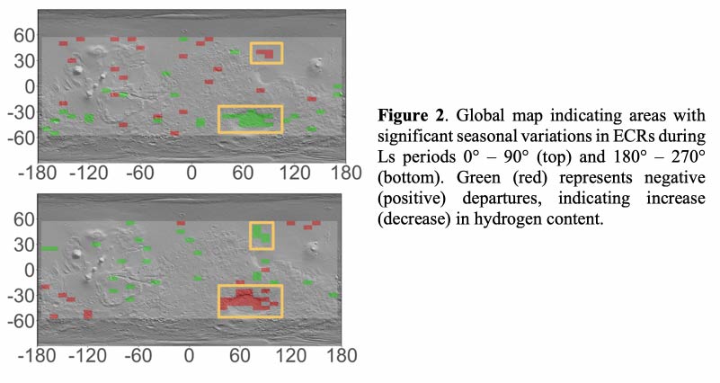
The relation between the seasonal variation in ECRs and the ground temperature retrieved from TES and THEMIS at Hellas Planitia and Utopia Rupes (not shown here) indicates that the coldest ground temperatures occur at the same time as the largest increase in hydrogen content is observed (and vice versa), suggesting that water ice might form in the shallow subsurface of these regions during the cold season, and then sublimating during the warm season of each hemisphere. Using modeling and satellite observations, we plan to investigate whether the magnitude and timescale of the observed seasonal changes in ECRs are consistent with changes in water ice, chemisorbed water, or physisorbed water.
Conclusions and Significance: Only Hellas Planitia and Utopia Rupes (Fig. 2) undergo a statistically-significant variation in ECRs (and therefore in the hydrogen content in the first meter of their subsurface). This variation is correlated with temperature in both regions, supporting the hypothesis that shallow subsurface water ice might form and sublimate during the cold and warm seasons of each hemisphere. These results are potentially important for future human exploration of Mars, as shallow subsurface water ice far from the poles is key for ISRU.
References: [1] Mesick, K. E., et al., Icarus 335 (2020): 113397. [2] Feldman, W. C., et al., J. Geophys. Res.: Planets 109.E9 (2004). [3] Wilson, J. T., et al., Icarus 299 (2018): 148-160. [4] Jakosky, B. M., et al., Icarus 175.1 (2005): 58-67.
How to cite: Martinez, G., Segura, A., Smith, M. D., Fischer, E., and Renno, N. O.: Looking for Non-Polar Shallow Subsurface Water Ice in Preparation for Future Human Exploration of Mars , Europlanet Science Congress 2021, online, 13–24 Sep 2021, EPSC2021-443, https://doi.org/10.5194/epsc2021-443, 2021.
Liquid water is one of the most important component in the search for potential extraterrestrial life, with Mars being a high priority target. However, the present martian conditions do not allow large scale pure liquid water formation on its surface (Haberle et al., 2001); most of the studies point to ephemeral emergence (e.g. Brass et al., 1980; Knauth et al.; 2002; Mellon et al., 2000; Kereszturi et al., 2009}, but there are theoretical studies proposing a longer presence (e.g. Clow et al., 1987; Hecht et al., 2002). Transient formation of salty brines is a feasible candidate for water formation, as multiple martian rovers have already identified perchlorate salts on Mars (Hecht et al., 2009; Navarro et al., 2010; Leshin et al., 2013; Ming et al., 2014). Since perchlorates are hygroscopic, they can form aqueous solutions if the temperature and relative humidity is suitable through a process called deliquescence (Gough et al., 2011; Gough et al., 2014; Fischer et al., 2014; Nuding et al., 2014; Zorzano et al., 2009).
The relative humidity was calculated with surface temperature, atmospheric pressure and water vapor volume mixing ratio data from Laboratoire de Météorologie Dynamique Mars General Circulation Model (LMDZ GCM) version 5. This climate model is detailed in Hourdin et al. (2006) the second generation of the model described in the works of Sadourny et al. (1984) and Forget et al., (1999). The data were simulated for the Mars year 29. To derive the relative humidity with respect to ice and with respect to liquid, the saturation water vapor volume mixing ratio was calculated with an equation based on the Goff-Gratch equation (Goff & Gratch, 1946; List,1984). For the detailed calculations please refer to the methods section of Pál et al. (2020).
Consider the instances, when every necessary circumstances were met except for one. Summing these cases up and taking a look at the statistics, we can get a clearer picture of the limiting circumstances according to time and location (Fig. 1, Fig. 2). The local times taken into consideration were between 9 PM and 5 AM. The reason for this is that outside this time frame, the chance for deliquescence is considerably lower. The percentages are calculated with respect to every single location between 80°N - 80°S and time; for example 35 % of dry scenarios mean that compared to all instances (43 latitude gridpoints, 65 longitude gridpoints and 669 sols totaling 1 869 855 cases), 35 % of them (approximately 654 449) fell into the dry scenario.
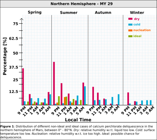
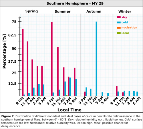
If we examine the Mars year 29 and separate the data by hemispheres and by seasons, the data suggests that most of the time relative humidity is the primary limiting factor. Even though the temperature is above the necessary eutectic temperature, the relative humidity remains too low (dry scenario). This is a substantially more frequent case, than the instances, when either the relative humidity with respect to liquid is high enough with too low temperatures (cold scenario), or the relative humidity with respect to ice is too high, favoring nucleation instead of deliquescence (nucleation scenario).
Separating by seasons, the local spring and summer show much higher percentages of being too dry with sufficient temperatures. Besides, the local spring and summer in the northern hemisphere show the highest chance for deliquescence (ideal scenario) between 9 PM and 3 AM. There is a similar trend in the southern hemisphere, but with overall lower percentages and mostly between 11 PM and 3 AM. In the southern hemisphere between 1 AM and 5 AM the instances for too cold scenarios also increase, resulting in a 8-15 % chance.
There is one particularly interesting time, which is 1 AM in the southern hemisphere, during the local autumn. At this time the percentage for too cold scenarios is 74.6 %, an obvious outlier compared to all the other cold cases. If we take a look at a close-up between sol 1 and sol 194 at the southern hemisphere at 60°S, 1 AM local time, the relative humidity is elevated between sol 1 and sol 80, the beginning of the local autumn (Fig. 3). This elevation is visible at all latitudes, 60°S was selected as an illustration. Comparing the 1 AM data with 11 PM and 3 AM data, in the latter cases the relative humidity is still elevated at the beginning of the year, but not enough to stay above the necessary minimum level for calcium perchlorate. At the same time, the surface temperature remains strictly below the eutectic temperature (Fig. 4), thus we arrive at the 74.6 % of cold scenarios.
Overall the data suggests that relative humidity is the main limiting factor to deliquescence during local spring and summer in both hemispheres. The percentages, where surface temperature was high enough with relative humidity w.r.t. ice still low enough is considerably higher, than the other scenarios (too cold or nucleation). The northern hemisphere seems more favourable between 9 PM and 3 AM, while in the southern hemisphere between 1 AM and 3 AM are suggested as more ideal times. From the hemispherically and seasonally averaged data we can conclude, that the overall chance for ideal periods is still rather low, but usually not zero. Reviewing local “hot spots for deliquescence” might be a good follow up to these results.
How to cite: Pál, B. D. and Kereszturi, Á.: Trends and key limiting factors of calcium perchlorate deliquescence on the surface of Mars, Europlanet Science Congress 2021, online, 13–24 Sep 2021, EPSC2021-162, https://doi.org/10.5194/epsc2021-162, 2021.
- Introduction:
Small cones are common on Mars. Many cones form chains several kilometers in length. The mechanisms of their formation are not explained. Cycloid forms are observed in a few places. Their origin is also unknown.
We consider a small region in Chryse Planitia where several chains of cones are found – Figs. 1, 2, 3. The cones height are ~20 m. The considered region is at the boundary of smooth plain on west (AHcs) and complex unit (AHcc) on east. The small region (HNck) in north-west corner of figure is the “older knobby material” – [1]. AH means Amazonian-Hesperian and HN - Hesperian-Noachian. The region is covered by lacustrine deposits. Some volcanic activity was possible in HNck.

Fig. 1. Our region in Chryse Planitia. Its part is presented in map at Fig. 2 (white rectangular, bold dashed line). The region is at the boundary of smooth plain (AHcs) and complex unit (AHcc) – Rotto and Tanaka (1995). The dotted black arrow a3 indicates structure presented in Fig. 4. The cycloid arcs are marked with letters c.
- Our hypothesis of cones origin:
Generally we consider 3 mechanisms of these cones formation: (i) a grains’ ejection, (ii) from mud or fluidized sand and (iii) explosive formation. Of course, the cones may be formed by several processes.

Fig. 2. Topography of the region shown in the dashed rectangle in Fig. 1. Topography is based on MOLA/HRSC Blended Digital Elevation Model 200 m on THEMIS Day IR layer. Data resolution is rather low, therefore, some smaller structures may not be visible on the map and non-existent artifacts may be found.
The chains labeled 1, 2, 3, 4, 5 are probably formed along outcrops of aquifers. The chains 7 and 8 of cones follow the course of valleys quite well. Therefore, it is difficult to expect that these cones are of igneous volcanism. Our hypothesis predicts the following scenario: (i) the regolith at the valley floor contained significant amounts of water left over from the floods. (ii) In the next stage, there was an overflow of lava in the vicinity of the area (HNck). This lava flowed into the valley creating a series of rootless cones. The material ejected by the explosion covered the valley and the slopes of the neighboring hills. (iii) Later, the lower structures (including the valley floor) were covered with fine aeolian sediments. This scenario is confirmed by thermal inertia observations.
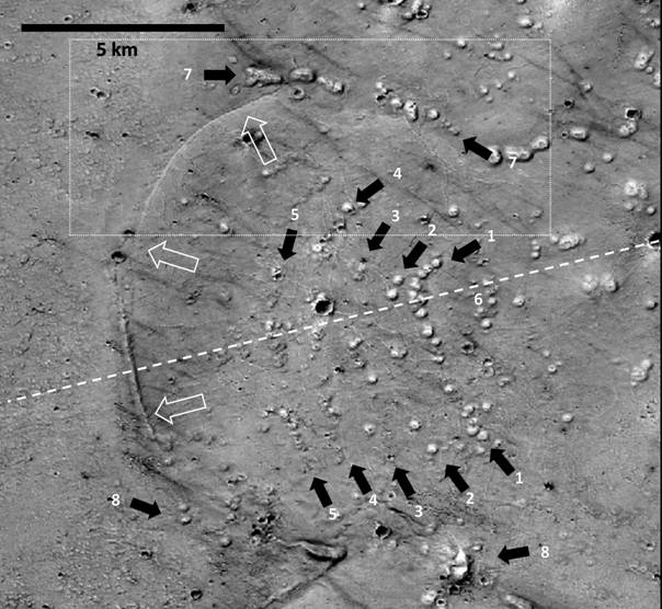
Fig. 3. The part of considered region (see Fig. 1). The chains of cones are indicated by solid black arrows and labeled by numbers 1, 2, 3, 4, 5. According to one of our hypotheses, some of these chains were formed along the outcrops of sediments with high content of volatiles. The chains of cones 7 and 8 may have been formed as rootless cones at the bottom of the valleys (side channels). The open arrows indicate the part of cycloid. NASA, P22_009485_2187_XN_38N040W.
- The cycloid
Consider now the structure extending north of the impact crater marked C1 in Fig. 1. It is a cycloid-like structure. It is marked by letters 'c'. It runs mostly on the western slopes of the hills - Fig. 2.
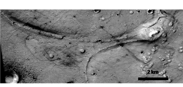
Fig. 4. The place where two cycloids meet. Note small cones on both arcs and the fact that both arcs run at the same height. This is an enlargement of part of Fig. 1 (arrow a3). NASA, CTX image P22_009485_2187_XN_38N040W.
Most cycloid arcs do not touch each other because they are separated by the side channels.
Let us consider Fig. 3. In the southern part of the hill there is no well-defined cycloid. One can see only several cones placed at the foot of the hill. This may be a result of the destruction of the original structure of cycloid during formation of cones. In the middle part, we observe a narrow embankment on the slope that is running approximately at halfway up the hill. The best preserved cycloidal structure is seen (as a belt of ~100 m wide) only since the end of the embankment (i.e., on northern part of Fig. 3). The belt runs approximately horizontally along the contour of the hill. The cycloidal arcs may be outcrops of a layer making up parts of the adjacent hills.
This possibility is supported by morphology seen in Fig. 4. It shows the confluence of adjacent arcs of cycloid. Both arcs are covered with small cones and extend at the same height. They could be outcrops of the same layer.
Also note that the cycloid arc on the hill shown in Fig. 3 lies at the same height as chain of cones 1. So maybe the cycloid arc and the chain 1 lay along outcrops of the same layer. Arc of cycloid is an outcrop on the west slope, while chain 1 marks an outcrop on the east slope of the hill. The lack of larger cones on the arc of cycloid could be a result of less intensive heating or lower amount of volatiles in western part of the layer comparing to eastern part.
The arcs marked with 'd' in Fig. 1 seem to be similar to the cycloid arcs discussed above. However, the topography of the area along the 'd' arcs is significantly different, so we conclude that such statement is premature.
- Conclusions;
Two different origins of cones we suggest: along outcrops of aquifers and as rootless cones [2]. The cycloid could be also a result of activity along outcrops of aquifers.
Acknowledgments: This study was supported by statutory project of Institute of Geophysics of University of Warsaw. We are also grateful to prof. W. Kofman and dr. J. Ciążela for their remarks.
References
[1] Rotto, S., Tanaka, K. L. (1995) Geologic/ geomorphologic map of the Chryse Planitia: region of Mars. USGS. [2] Czechowski L., et al. (2020), Cones chains in Chryse Planitia and some thermodynamic aspects of their formations. submitted.
How to cite: Czechowski, L., Zalewska, N., Zambrowska, A., Ciazela, M., Witek, P., and Kotlarz, J.: Chains of small cones and a cycloid form at Chryse Planitia on Mars, Europlanet Science Congress 2021, online, 13–24 Sep 2021, EPSC2021-434, https://doi.org/10.5194/epsc2021-434, 2021.
Introduction: There are thousands of small cones on Isidis Planitia on Mars. The cones have diameters of 300–500 m and heights of ~30 m. Many cones form subparallel chains several kilometers in length. Their origin is discussed in many papers [1,2,4,5] however, the mechanism of their formation is not explained, nor the reason for their arrangement in subparallel chains. The cones may be: rootless cones, cinder cones, tuff cones, pingos, mud volcanoes etc. [5]. Some of chains have a characteristic furrow suggesting possibility of fissure volcanism.
The prevalence of these chains indicates that large-scale processes are responsible for their formation. Their proper classification can help identify their origin and explain other large-scale processes on Isidis Planitia. There are a few works about statistics of cones on Isidis Planitia e.g. [1,2,3]. However, we approached the problem in a different way.
Considered region: Our analysis indicates that the cones can be grouped in larger systems. We divided Isidis Planitia into several characteristic regions (Fig.1). There may be several types of cones in one of the distinguished regions. Our division is based on the following structures (Fig. 2):
1. Chains of separate cones,
2. Chains of cones connected with each other,
3a. Chains of cones connected to the furrow through the center,
3b. Chains of cones connected to the furrow through the center with elongated, elliptical cones
4. Chains of cones with the traces of flows,
5. Chains of irregular cones without calderas with a depression around the cones,
6a. Ridge arches without cones,
6b. Chains of cones on the ridges.
In the division of Isidis Planitia shown in Fig. 1, we also paid attention to the orientation of the chains of cones (Fig. 2). The sense of black arrows in regions is explained in Fig. 3 and in the text below. In most of our regions there are also groups of cones that do not form linear chains. Such group are named as "field of cones".
Our current Isidis Planitia division includes 36 regions. We distinguished 11 regions with the predominant arrangement of arcs in the directions between ENE and ESE outlined in yellow (see Fig. 1 for notation of directions), 5 regions with the directions between WNW and WSW outlined in orange, 2 regions with the directions between NNE and NNW outlined in magenta and 15 areas with the directions between SSE and SSW, outlined in purple. 3 regions where the arcs of the cones are concentric (chains have common centers) are outlined in red. These 36 regions cover substantial part of the Isidis Planitia. In the rest of our regions there almost are not chains of cones.
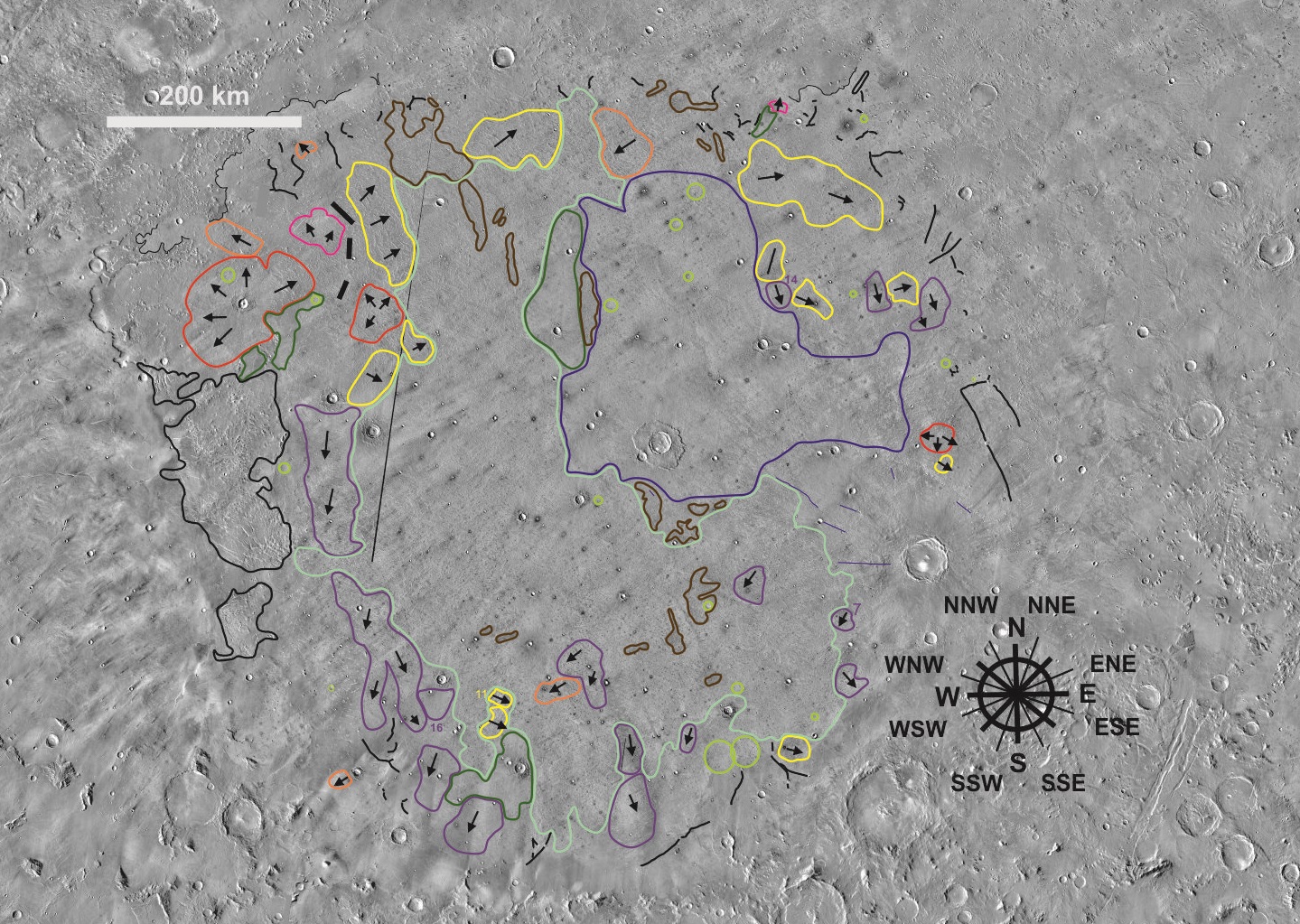
Fig.1. Regional division of the Isidis Planitia (THEMIS background) based the predominant direction of cones chains. Description of the regions in the text.
Except for the regional analyses, we have also mapped sinuous ridges (marked black, winding lines), cracks and serial depressions, occurring near craters (marked blue lines), fields with polygonally cracked surface (outlined in black line), areas with a large number of small craters (outlined in brown ), areas with few or no cones (outline in green) and quasi-circular depressions sQCDs called ghost craters [5] (marked light green circle) (Fig. 1).
In addition, we distinguished a large area without subparallel arcs with chaotic chains (outlined in cyan) and another large area with groups of cones creating fields, not forming chains, (outlined in navy blue).
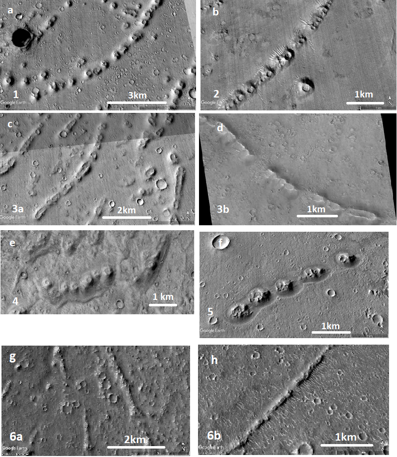
Fig.2. Various sets of cones in the Isidis Planitia: a) Chains of separate cones, b) Chains of cones connected with each other, c) Chains of cones connected to the furrow through the center, d) Chains of cones connected to the furrow through the center with elongated elliptical cones, e) Chains of cones with the traces of flows, f) Chains of irregular cones without calderas with a depression around the cones, g) Ridge arches without cones, h) Chains of cones on the ridges. The images are mosaic CTX except for d) which is based on HiRISE, ESP_013054_1900.
Analysis of terrestrial analogues: We consider terrestrial analogues, hoping that they will show us possible mechanisms of the formation of cone chains on Mars. We chose such following analogues: glacial eskers [1], cinder cones, submarine volcanoes and rootless cones (Fig.3). Isidis cones are currently studied for the genesis of individual types of cones. We believe that volcanic origin (the result of lava flows) or phreatic origin (cones are form by solid pyroclastic material) are probable. Characteristic furrows in some chains suggest fissure volcanism.
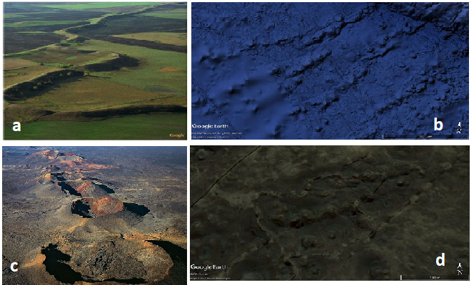
Fig.3. Selected terrestrial analoues of linear structures: a) eskers at Mc Donald Lakes, British Columbia, Canada, b) submarine volcanic cones in the Middle America Trench and the Tehuantepec Transform/Ridge, c) cinder cones on Lanzarote, Timanfaya National Park, www.lowcosttourslanzarote.com/blog/lanzarote-highlights/1-national-park-of-timanfaya, d) rootless cones on in the Landbrot, Iceland.
Conclusions: Our division is made according to consistent characteristic morphological features. The next stage of the work will be to explain the mechanism of the formation of these forms, based on known geological phenomena but in relation to Mars. We want to clarify whether the designated areas were created in the same geological processes, or whether a different mechanism is responsible for the differences in these forms. We suspect that the chains 1, 2, 3a and 3b were created in a similar way but with different intensity of the processes. On the other hand, the chains 6a, 6b and 4 and 5 could have arisen in a different geological process.
References:
[1] Guidat, T., et al., (2015) Earth and Planet. Sci. Let . 411, 253-267. [2] Souček, O., et al., (2015) Earth and Planet. Sci. Let 426, 176-190. [3] Hiesinger H., et al., (2009) 47th Lunar and Planet. Sci. Conf. 2767. [4] Gallinger, C.L. and Ghent, R.R,. (2016) 40th Lunar and Planet. Sci. Conf. 1953. [5] Ghent, R. R., et al., (2012) Icarus 217, 1169-183.
How to cite: Zalewska, N., Czechowski, L., Ciążela, J., and Kuzaj, M.: Regional and local geological characteristics of Isidis Planitia on Mars and analysis of terrestrial analogues., Europlanet Science Congress 2021, online, 13–24 Sep 2021, EPSC2021-446, https://doi.org/10.5194/epsc2021-446, 2021.
The last two decades have seen a growing number of Martian orbital missions with optical cameras of a various range of resolution. The topographic context of these images is crucial to decipher Martian surface processes. Thanks to stereo-photogrammetry, digital elevation models (DEM) can be produced from couple of images taken from different view angles.
MarsSI [1] is a french Research Infrastructure that allows the users to easily and rapidly select observations, to process raw data via proposed automatic pipelines and to get back final products which can be visualized under Geographic Information Systems. MarsSI provide automated DEM generation based on the Ames Stereopipeline software (ASP) [2].
DEM generation
The previously used workflow, which was used until the 1st of may, 2020, of MarsSI DEM pipeline was a straightforward use of ASP to create a DEM that would be fitted against the global MOLA DEM dataset to account for orbital imprecision in elevation and referencement. We were however not satisfied with the alignment results and artefact levels in the results.

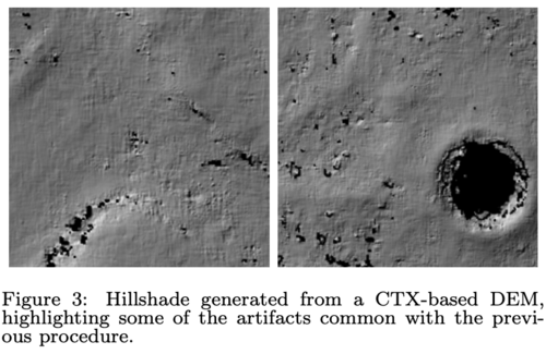
To optimize the pipeline, we first enable a bundle adjustment phase to improve future correlation between left/right image. We then consider our correlation options. Recent versions of ASP allowed to use the semiglobal matching (SGM) and derived correlators. Mars often present smooth and featureless areas that yield poor results for the traditional correlator function. The SGM correlator is a relevant way to address this issue, being able to find a correlation solution with smaller window size, which also improve computational times.
Camera models and correction are provided within ASP, as well as images reprojection using an existing DEM to account for the topography. We consider using the MOLA dataset as the reference, but approximate orbital positions means that we will not match inputs to their exact position (sometimes by a few thousand meters) and introduce errors. One solution in that case is to first create a low resolution DEM with the input images we intend to use. Since at the beginning of the DEM creation, we match and align input images, this DEM fit them well despite having an approximate map-projection. Outputting this DEM at lower resolution minimize the correlation errors. We also enable missing data filling at this point by applying large maximum search distance method, to avoid loosing data from input images. This give us a result of enough quality to correct topography in the input images. We can then use these corrected images to create the high resolution DEM. During this phase, we decrease the filtering parameters compared to the first step. The result is a less smoothed DEM having sill few artefacts.


We also aim to improve the alignment of the produced DEM to the MOLA dataset. This step can be accomplished by ASP’s pc_align tool. One of the first issue we have is the resolution gap between MOLA and our DEM so that alignment is a challenge. To mitigate this aspect, we switch our reference from pure MOLA reference data to the blended HRSC+MOLA dataset (200m/px). We also highligth that pc_align works best when outlier measurements can be filtered. This is usually done by invalidating points that have a distance above a threshold between the dataset and the reference. Since our orbital-based georeferencing error is quite limited, by simply vertically prealign the data and using the fast global registration algorithm , the result is improved. Using fast global registration would also mean that even if the alignement fails, it would still prevent large errors to be introduced at this step.
With only minor parametrization differences, we applied the same workflow for both CTX and HiRISE imagery. Most notably, we applied stricter alignment maximum distance replacement.
Oxia Planum mosaics
Aside improving the overall quality of individual products, we also designed this new workflow having in mind to create mosaic of consistant, properly aligned to a common reference, datasets.
We proceed to apply this method to 32 pairs of HiRISE imagery located on the ESA ExoMars2022 landing site, 24 of which were successfully generated. Alongside the DEM, we use ASP functions to generated a corresponding reprojection of the left image with the aim to produce both a DEM and an orthorectified imagery mosaics.
However, while we find our alignment procedure to have a precision good enough for CTX scalemosaicking of products, automated HiRISE products alignements did not achieve an acceptable level. In addition to the previous workflow, we first coregistered a CTX mosaic at 10m/px against a HRSC mosaic processed and provided by the DLR[9]. This CTX mosaic was used t o align the HiRISE products whom coregistration was then refined again, manually, using ground control points against the corresponding orthorectified HRSC imagery corresponding to the DEM.


This data was used in the context of the geological mapping exercice conducted by ESA in the summer of 2020 for the Exomars2022 mission and was the primary high-resolution layer used in the MMGIS environment deployed by ESA.
Conclusion
This work allows the MarsSI infrastructure to produce DEM of greater quality that will also fit better in GIS environments, while requiring no user input. We now can also consider the automated production of mosaics using CTX data, and with user input for HiRISE data. While more time-consuming, this allowed us to provide a useful hi-resolution dataset for the mapping exercise of the Exomars2022 project.
Data DOIS
10.48326/IDOC.PSUP.MARSSI.CTX.OXIA
10.48326/IDOC.PSUP.MARSSI.HIRISE.OXIA
References
-
C. Quantin-Nataf, L. Lozac’h, P. Thollot, D. Loizeau, B. Bultel, J. Fernando, P. Allemand, F. Dubuf- fet, F. Poulet, A. Ody, H. Clenet, C. Leyrat, S. Harrisson, MarsSI: Martian surface data process- ing information system, Planetary and Space Sci- ence 150 (2018) 157 – 170, ISSN 0032-0633, doi: https://doi.org/10.1016/j.pss.2017.09.014.
- R. A. Beyer, O. Alexandrov, S. McMichael, The Ames Stereo Pipeline: NASA’s open source software for deriv- ing and processing terrain data, Earth and Space Science 5 (9) (2018) 537–548.
How to cite: Volat, M., Quantin-Nataf, C., and Dehecq, A.: An overview of MarsSI new DEM workflow and resulting Oxia Planum mosaics, Europlanet Science Congress 2021, online, 13–24 Sep 2021, EPSC2021-163, https://doi.org/10.5194/epsc2021-163, 2021.
Geological investigations of planetary surfaces require the combination of orbital datasets. Missions being often multiple-instruments platforms from multiple space agencies, the quantity of data available increased quickly.
MarsSI [3] is a platform designed to explore, calibrate, process and retrieve Mars orbital data. It was certified in 2017 as french national Research Infras- tructure by the Centre National de la Recherche Scientifique (CNRS) as part of the Planetary Surface Portal (PSUP) [2].
As of 2021, it indexes the optical (visible, multi and hyper-spectral) data from the recent orbiter missions, and allow to request the creation of Digital Elevation Models on demand. The focus, as highlighted by figure 1 is to allow the user to browse and request ”ready-to-use” products in regards of calibration, refinements and georeferencing. The user will be able to visualize and interpret the data in GIS or remote sensing software.
We are now presenting the new web interface that was introduced in a beta phase to the users in may 2021.
Overview
MarsSI original web interface was based on Geomajas (www.geomajas. org), a free and open source GIS toolkit. This allowed us to build an interface consisting in a map view to display and select products to be added to a workspace. A seperatate view would allow to request actions regarding the products in the workspace, such as “download”, “process”, “copy”.
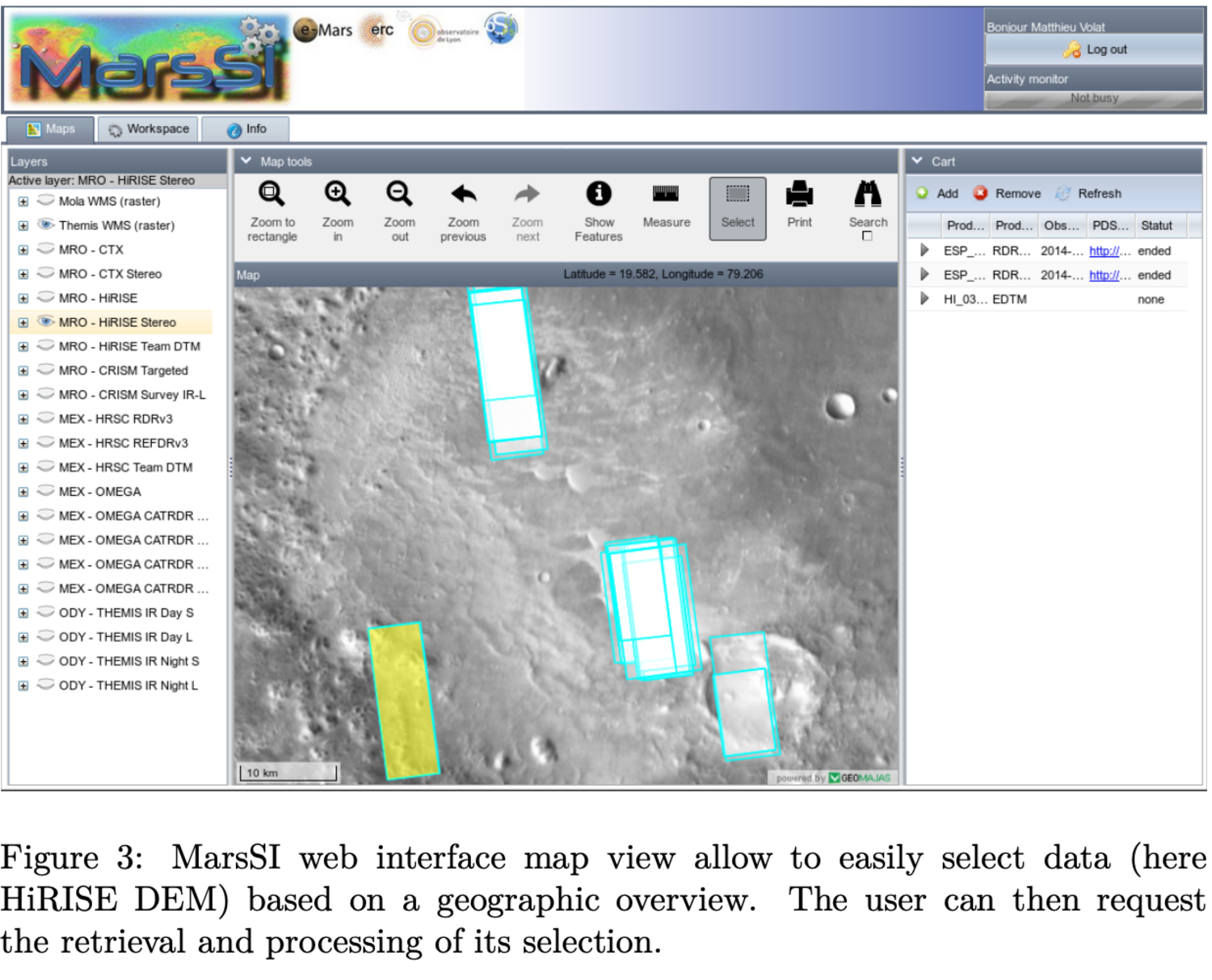
With time, we however have recognized the limitation of this toolkit. Developpement slowed down on the upstream project, and we found very hard to continue coding the whole project in Java. Client-side code was proving to be less and less compatible with web browsers, and did not allow use to natively use newer features that would either ease coding or improve user experience. Server-side code was very ressource-consuming, hard to debug and support for newer java version was inexistant for certain libraries.
New version
We selected to rely on the Python Django framework (www.djangoproject.com) to build our new web interface. This choice was motivated by the maturity of the project, the ease of developpement, configuration and deployment and safe dependency management. The design was based to use just the Javascript code necessary and not more : we elected to rely on the Leaflet framework to provide WebGIS functionnality due to being able to use our already-existing OGC backends. As of 2019, it was only the only framework we found to be able to use custom projections, something needed for planetary GIS.
Design-wise, we chose a simplified view, but kept a lot of the functionnal concepts of the previous version that were still relevant. We kept a system of tabs to switch between a Map view, a Workspace view and a Job view.
Our new map view maximise the space allocated to the map. We also created a new, better background layer of composite THEMIS/MOLA. The Murray Lab global CTX mosaic was also added as a background layer, as well as a nomenclature layer to display the IAU labels. Users will be able, as before, to display, select and add footprint to their workspace from there. We elected not to duplicate the workspace view in this tab.
 `
`
The search view is still a work in progress: we separated this functionnality in a tab that allow freetext search to return results. Footprints can be previewed from there, and product can also be added to provide minimal functionnality, but we expect to work more on this part in the near future.
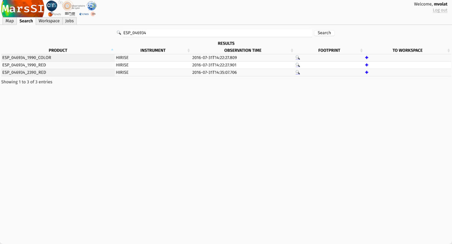
The workspace view is a consolidated view of the product selection. We present a table allowing to display some informations on the datasets, a footprint overwiew, some basic facilities to sort and search the entries. Products availability is displayed with a color code indicating the availability of the subproducts of an entry (for exemple, for an image: the raw EDR data, calibrated RDR, projected MRDR, etc). It is also from the workspace the user will select and request data processing or copy to its SFTP directory.
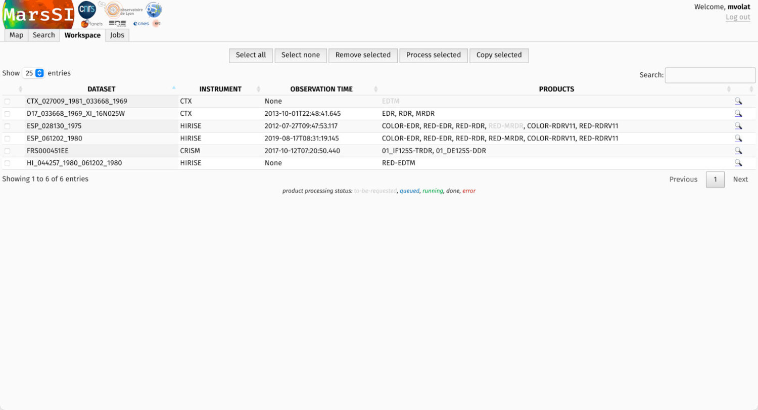
The job view allow to concentrate on the requests the user specified. Using the REST interface provided by our cluster batch management system, OAR (https://oar.imag.fr), it is a close view of MarsSI computationnal facilities. We also hope to develop this view to help understand better product processing.
We chose to not to try to integrate the wiki that can still be accessed as a separate page. A “getting started” page explain the basics of the new interface, other specific pages will be updated when this new “Django” version is MarsSI default web interface.
Conclusion and perspectives
We built a new interface to display and browse MarsSI catalog, request dataset processing and copies. This new interface make use of both web and cartographic standards to provide an elegeant and reliable service that also paves the way for more improvements.
We plan to improve usability both in map and search view, espcially when there is a great number of products to display. We are also already working on “context” views to present Mars polar view and display other planetary surfaces, and extend our facility beyond Mars.
How to cite: Volat, M. and Quantin-Nataf, C.: Presentation of the new web interface of MarsSI, the martian surface data service, Europlanet Science Congress 2021, online, 13–24 Sep 2021, EPSC2021-186, https://doi.org/10.5194/epsc2021-186, 2021.
Please decide on your access
Please use the buttons below to download the presentation materials or to visit the external website where the presentation is linked. Regarding the external link, please note that Copernicus Meetings cannot accept any liability for the content and the website you will visit.
Forward to presentation link
You are going to open an external link to the presentation as indicated by the authors. Copernicus Meetings cannot accept any liability for the content and the website you will visit.
We are sorry, but presentations are only available for users who registered for the conference. Thank you.
Please decide on your access
Please use the buttons below to download the presentation materials or to visit the external website where the presentation is linked. Regarding the external link, please note that Copernicus Meetings cannot accept any liability for the content and the website you will visit.
Forward to session asset
You are going to open an external link to the asset as indicated by the session. Copernicus Meetings cannot accept any liability for the content and the website you will visit.
We are sorry, but presentations are only available for users who registered for the conference. Thank you.