OPC applications
TP1 | Atmospheres and Exospheres of Terrestrial Bodies
EPSC2024-231 | ECP | Posters | TP1
Validation of Martian dust storm trajectories in the Mars PCM using observational datasetsMon, 09 Sep, 14:30–16:00 (CEST) | Poster area Level 2 – Galerie | P1
TP2 | Mars Surface and Interior
EPSC2024-748 | ECP | Posters | TP2 | OPC: evaluations required
Water and Sediment Transport Processes in Jezero CraterWed, 11 Sep, 10:30–12:00 (CEST) | Poster area Level 2 – Galerie | P7
EPSC2024-777 | ECP | Posters | TP2
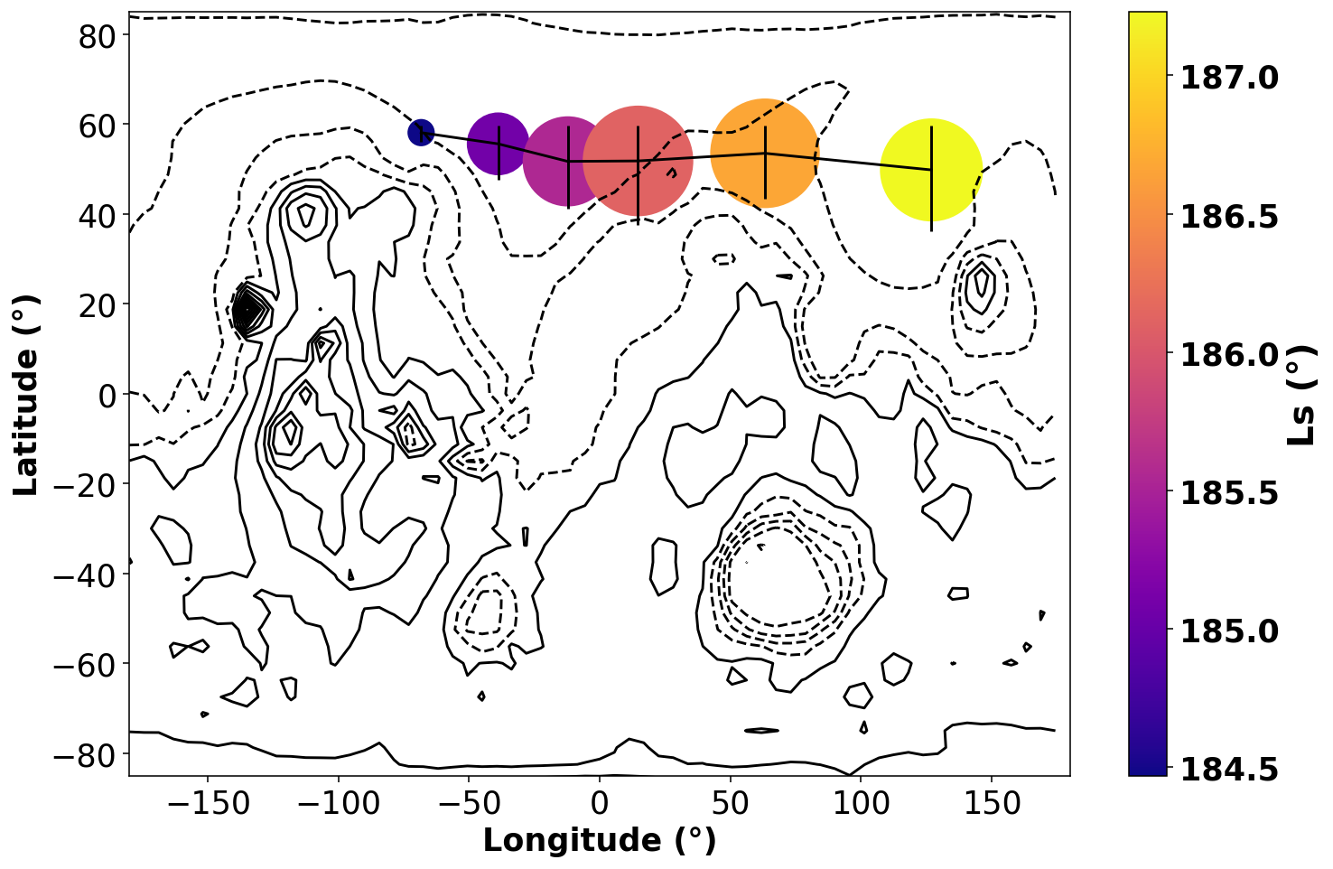
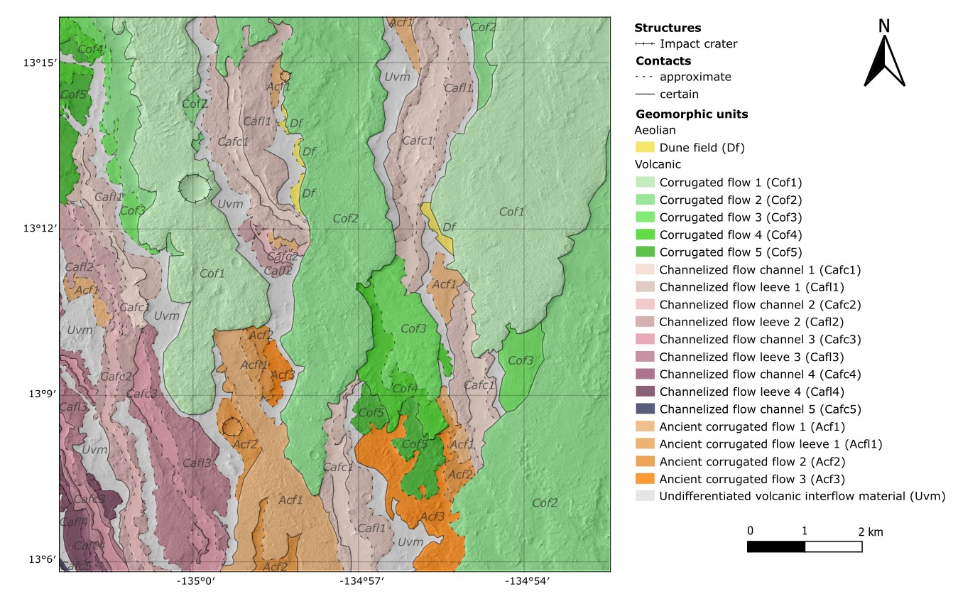
Polyphase Amazonian floods in the Olympica – Jovis Fossae channel system.Wed, 11 Sep, 10:30–12:00 (CEST) | Poster area Level 2 – Galerie | P14
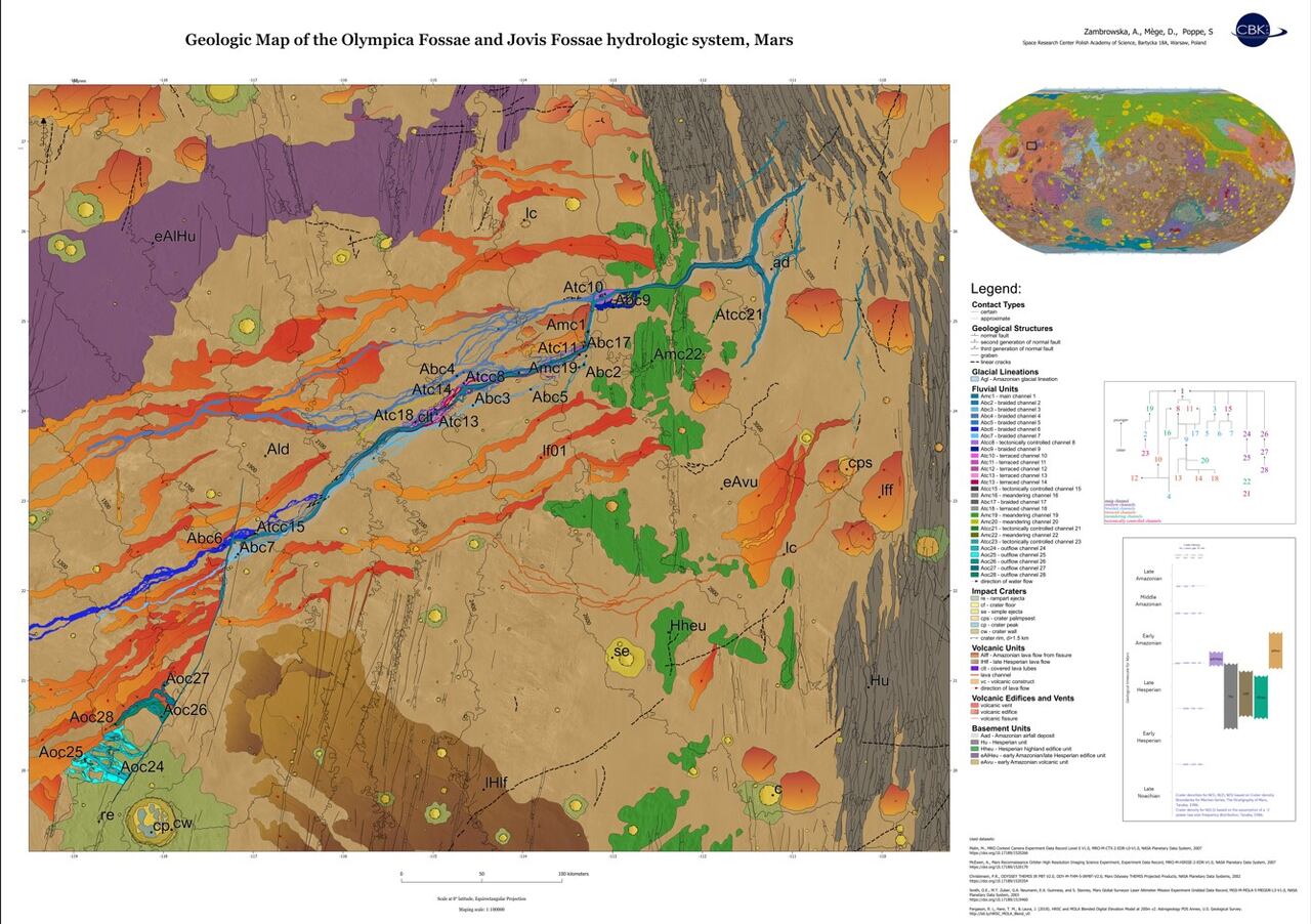
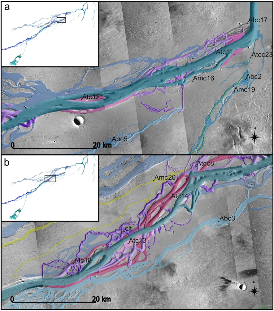
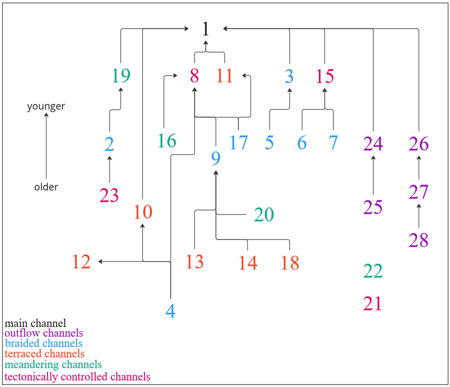
EPSC2024-1077 | ECP | Posters | TP2
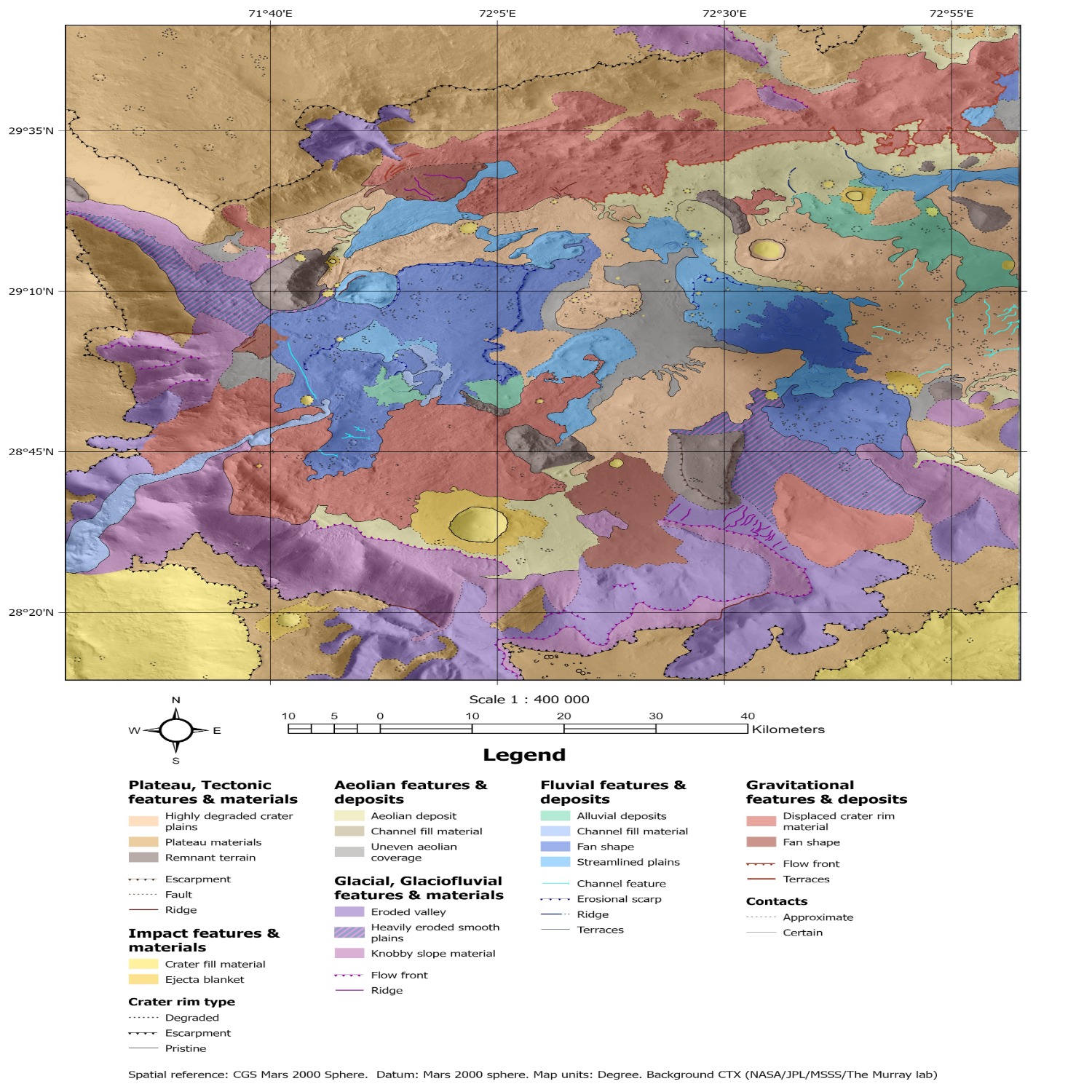
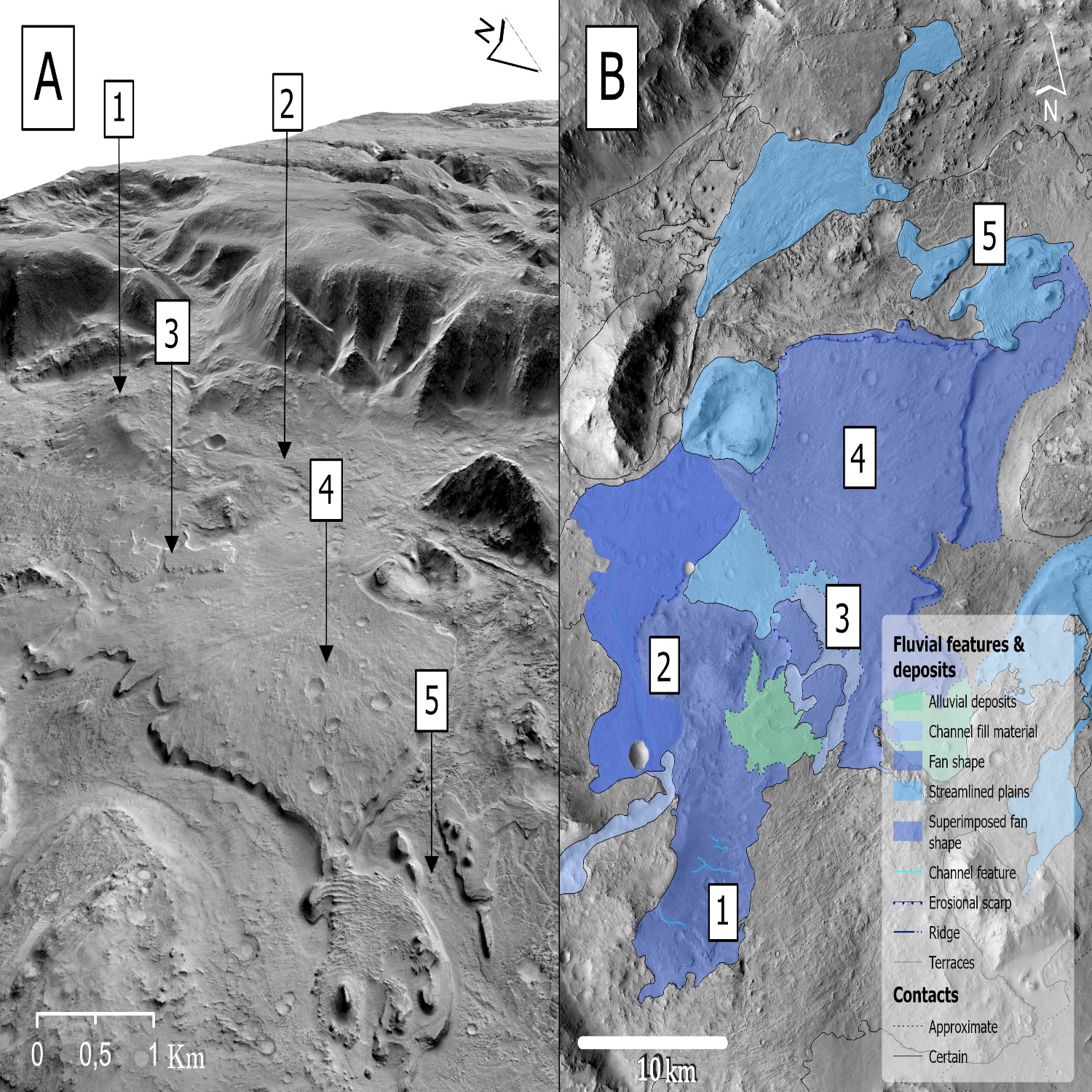
Evolution of fluvial, and possible lacustrine or marine activity in Nilosyrtis, Mars - A geomorphological & chronostratigraphic analysis.Wed, 11 Sep, 10:30–12:00 (CEST) | Poster area Level 2 – Galerie | P12
EPSC2024-1115 | Posters | TP2 | OPC: evaluations required
Exploring Polygonal Patterned Grounds in the Hyper-arid Atacama Desert: Insights into Formation Mechanisms and Implications for Martian AnaloguesWed, 11 Sep, 10:30–12:00 (CEST) | Poster area Level 2 – Galerie | P18
EPSC2024-1355 | ECP | Posters | TP2 | OPC: evaluations required
Spatiotemporal development of two stepped fans in Xanthe Terra and Terra Sirenum, MarsWed, 11 Sep, 10:30–12:00 (CEST) | Poster area Level 2 – Galerie | P9
TP3 | Planetary field analogues for Space Research
EPSC2024-124 | ECP | Posters | TP3 | OPC: evaluations required
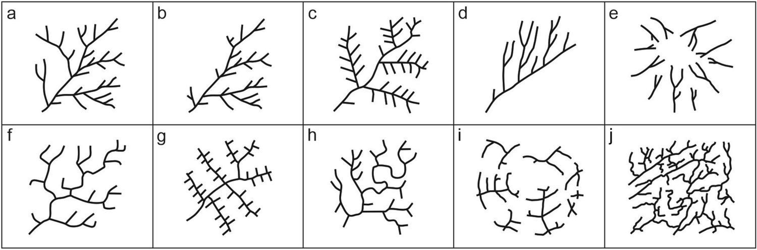
Rivers' classification: integrating Deep Learning and statistical techniques for terrestrial and extraterrestrial drainage networks analysisTue, 10 Sep, 10:30–12:00 (CEST) | Poster area Level 2 – Galerie | P10
EPSC2024-695 | ECP | Posters | TP3 | OPC: evaluations required
Mapping of Martian geomorphologies as a contribution to construct the first artificial analog in ColombiaTue, 10 Sep, 10:30–12:00 (CEST) | Poster area Level 2 – Galerie | P2
EPSC2024-914 | ECP | Posters | TP3 | OPC: evaluations required
Towards Low Earth Orbit Exposure Experiments on the ISS -Designing a Simulation Setup for Mars Like ConditionsTue, 10 Sep, 10:30–12:00 (CEST) | Poster area Level 2 – Galerie | P12
EPSC2024-982 | ECP | Posters | TP3
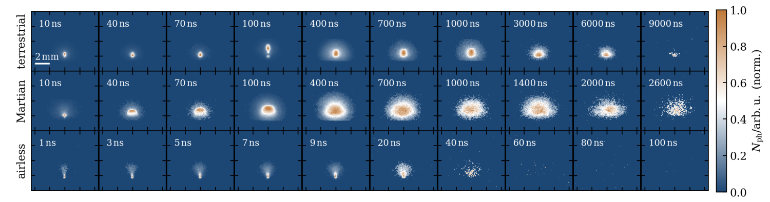
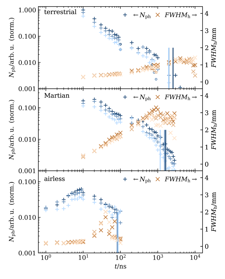
Charge Distribution of Ejected Particles after Impact Splash on Mars: A Laboratory ApproachTue, 10 Sep, 10:30–12:00 (CEST) | Poster area Level 2 – Galerie | P4
TP4 | Planetary Dynamics: Shape, Gravity, Orbit, Tides, and Rotation from Observations and Models
EPSC2024-952 | ECP | Posters | TP4 | OPC: evaluations required
Satellite gravity-rate observations to uncover Martian plume-lithosphere dynamicsWed, 11 Sep, 14:30–16:00 (CEST) | Poster area Level 2 – Galerie | P26
TP5 | Ionospheres of unmagnetized or weakly magnetized bodies
EPSC2024-34 | Posters | TP5 | OPC: evaluations required
Gravity Wave-Induced Ionospheric Irregularities in the Martian AtmosphereTue, 10 Sep, 14:30–16:00 (CEST) | Poster area Level 2 – Galerie | P23
EPSC2024-219 | ECP | Posters | TP5
Evolution of the ion dynamics at comet 67P during the escort phaseTue, 10 Sep, 14:30–16:00 (CEST) | Poster area Level 2 – Galerie | P27
EPSC2024-1287 | ECP | Posters | TP5 | OPC: evaluations required
Preliminary Results of the Categorizing and Statistical Survey of Martian Ionospheric IrregularitiesTue, 10 Sep, 14:30–16:00 (CEST) | Poster area Level 2 – Galerie | P26
TP6 | Late accretion and early differentiation of rocky planetary bodies, from planetesimals to super-Earths
EPSC2024-763 | ECP | Posters | TP6
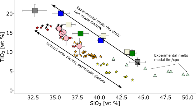
Resolving the origin of lunar high-Ti basalts by petrologic experimentsWed, 11 Sep, 10:30–12:00 (CEST) | Poster area Level 2 – Galerie | P35
EPSC2024-1006 | ECP | Posters | TP6 | OPC: evaluations required
1D Modeling of the Magma Ocean Stage of Rocky PlanetsWed, 11 Sep, 10:30–12:00 (CEST) | Poster area Level 2 – Galerie | P31
TP7 | Planetary volcanism, tectonics, and seismicity
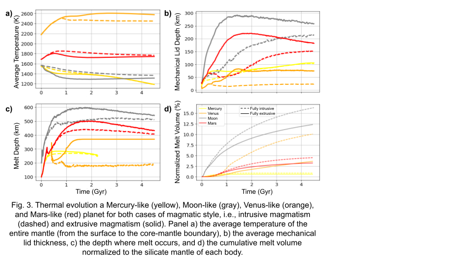
EPSC2024-650 | ECP | Posters | TP7 | OPC: evaluations required
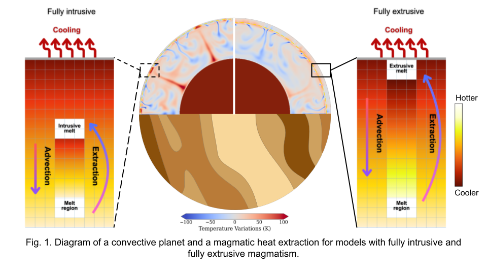
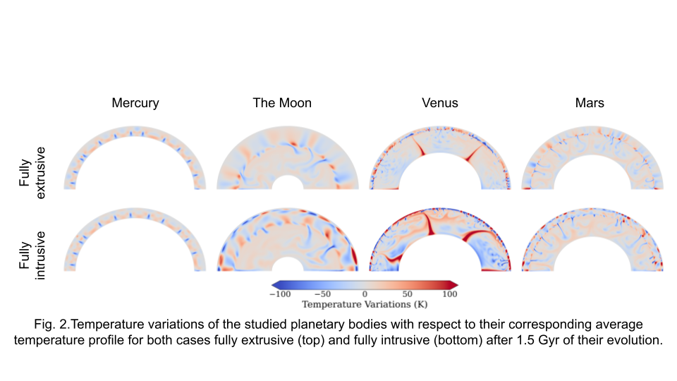
Effects of magmatic styles on the thermal evolution of planetary interiorsWed, 11 Sep, 10:30–12:00 (CEST) | Poster area Level 2 – Galerie | P44
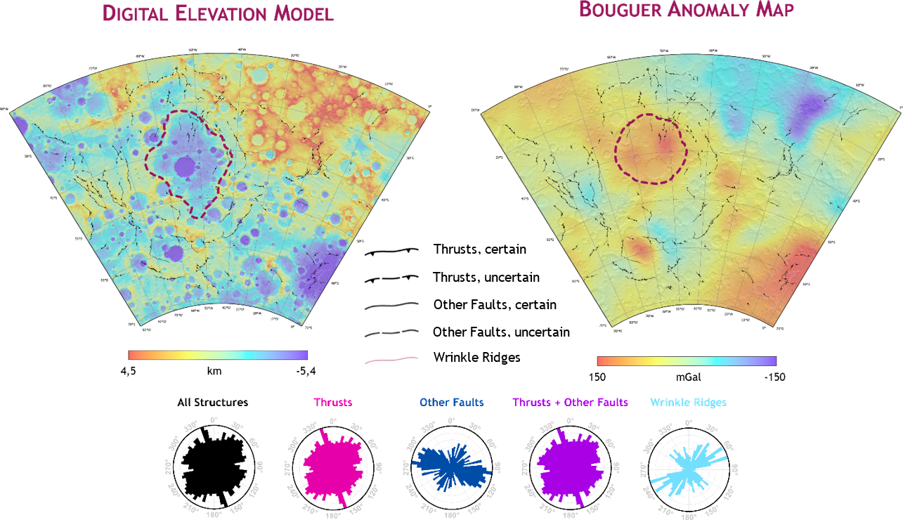
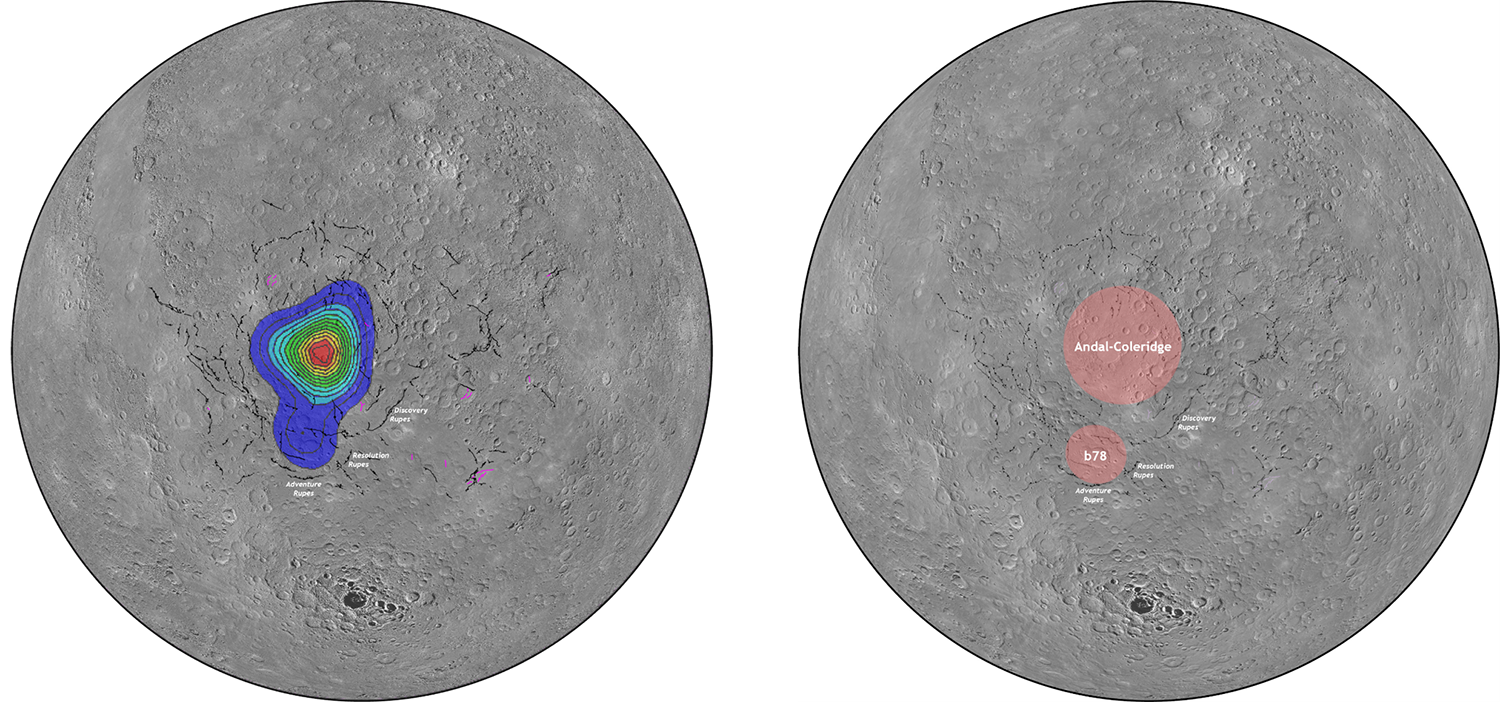
EPSC2024-1106 | ECP | Posters | TP7
Tectonic influence of multi-ring basins: The case of Mercury’s Discovery Quadrangle and the Andal-Coleridge basin.Wed, 11 Sep, 10:30–12:00 (CEST) | Poster area Level 2 – Galerie | P47

TP9 | Impact Processes in the Solar System
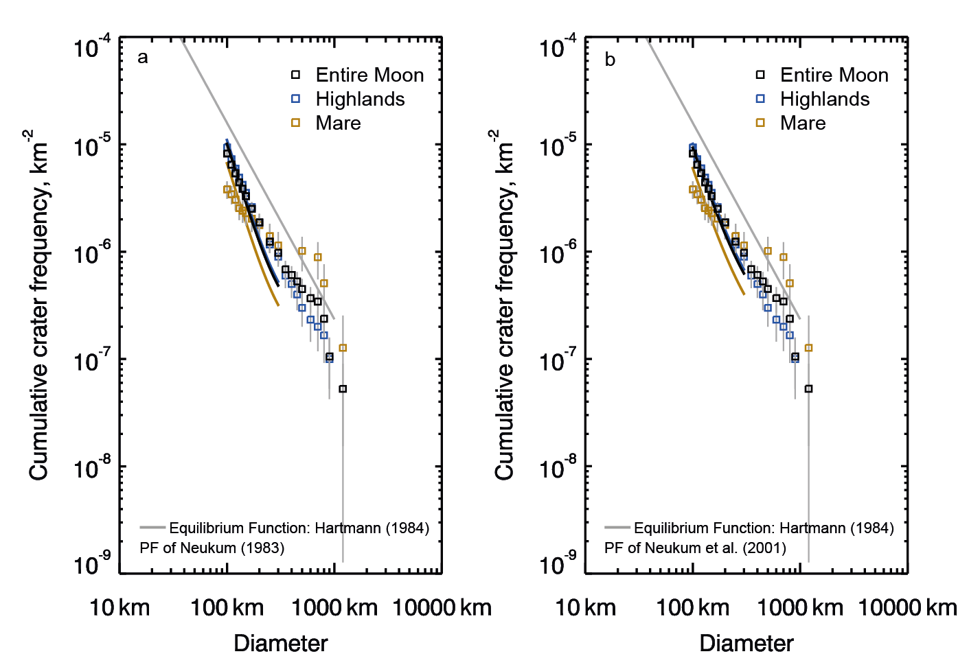
EPSC2024-372 | ECP | Posters | TP9 | OPC: evaluations required
Evaluation of large craters and basins for lunar production functionsThu, 12 Sep, 14:30–16:00 (CEST) | Poster area Level 2 – Galerie | P9
EPSC2024-437 | ECP | Posters | TP9 | OPC: evaluations required
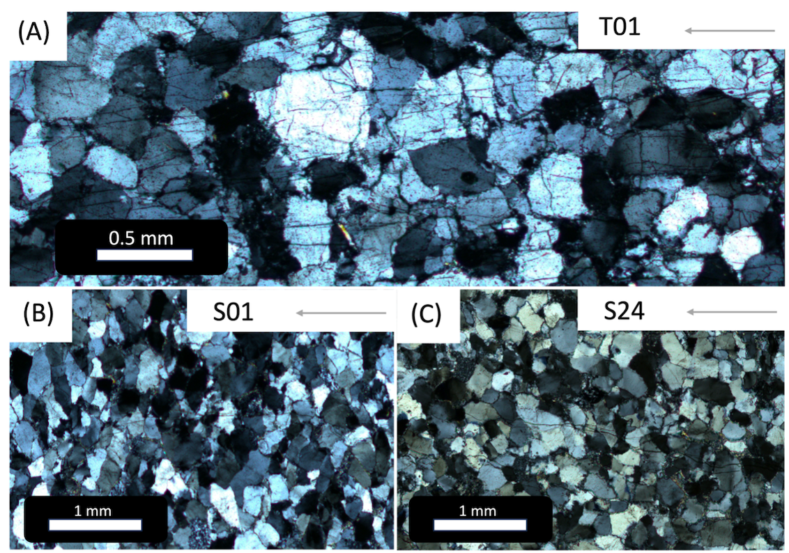
Efficacy of classical and spectroscopic techniques for strain quantification in weakly shocked rocks: Results from experimentally impacted Taunus quartziteThu, 12 Sep, 14:30–16:00 (CEST) | Poster area Level 2 – Galerie | P13
EPSC2024-560 | ECP | Posters | TP9 | OPC: evaluations required
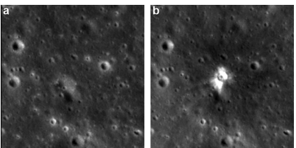
Modelling Lunar Impact Flashes from Molten EjectaThu, 12 Sep, 14:30–16:00 (CEST) | Poster area Level 2 – Galerie | P6

EPSC2024-956 | ECP | Posters | TP9 | OPC: evaluations required
From Debris to Resource: Simulating High-Velocity Impacts of Space Debris on the MoonThu, 12 Sep, 14:30–16:00 (CEST) | Poster area Level 2 – Galerie | P7
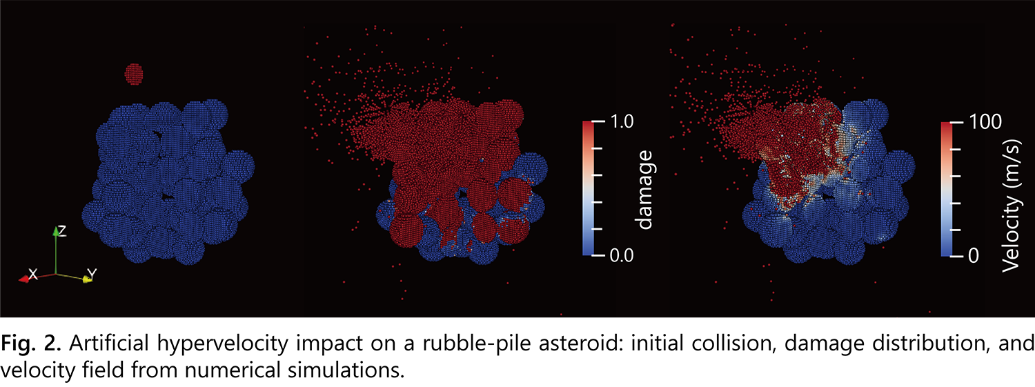
EPSC2024-1111 | ECP | Posters | TP9 | OPC: evaluations required
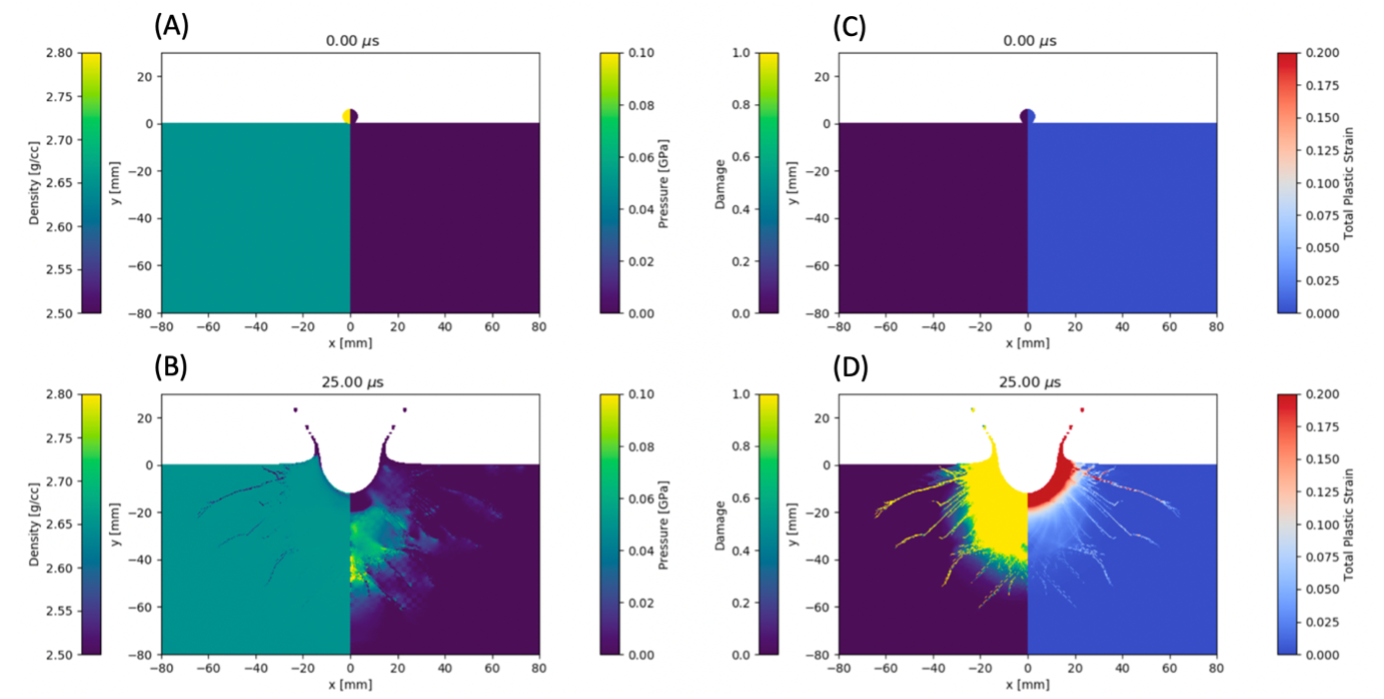
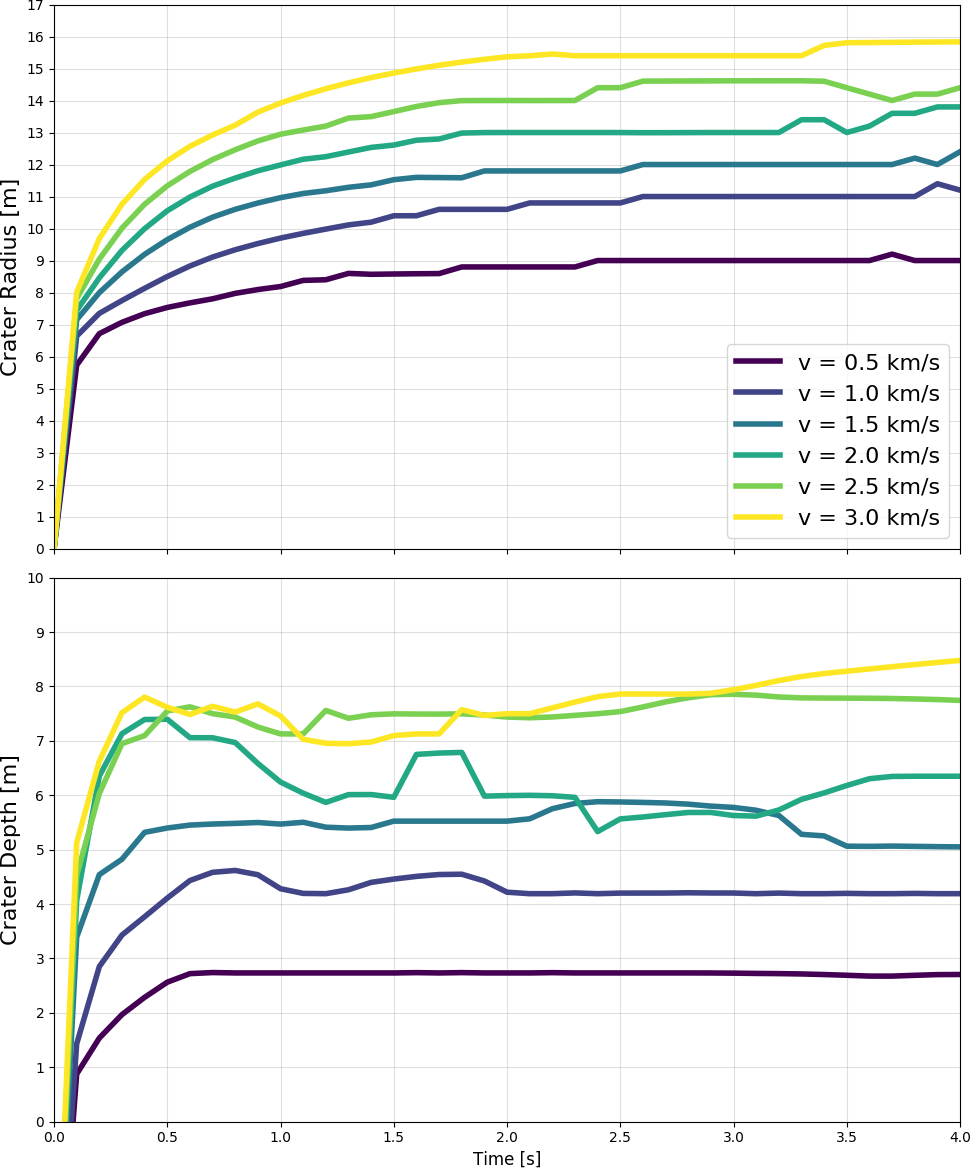
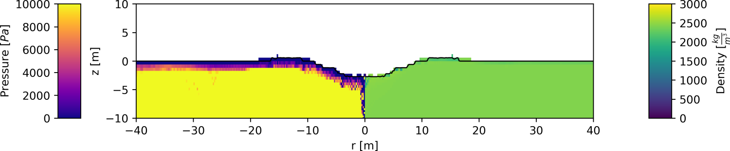
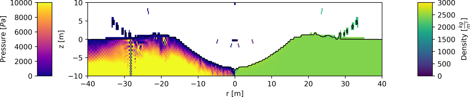
Quantifying the effect of asteroid structure on hypervelocity impact outcomes with the Material Point MethodThu, 12 Sep, 14:30–16:00 (CEST) | Poster area Level 2 – Galerie | P8
TP10 | Exploring Mercury and its environment
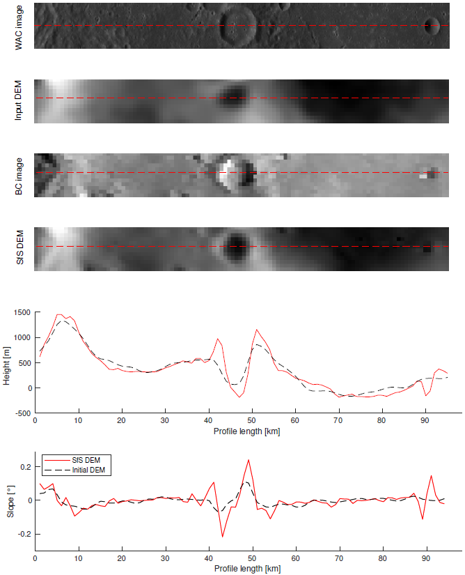
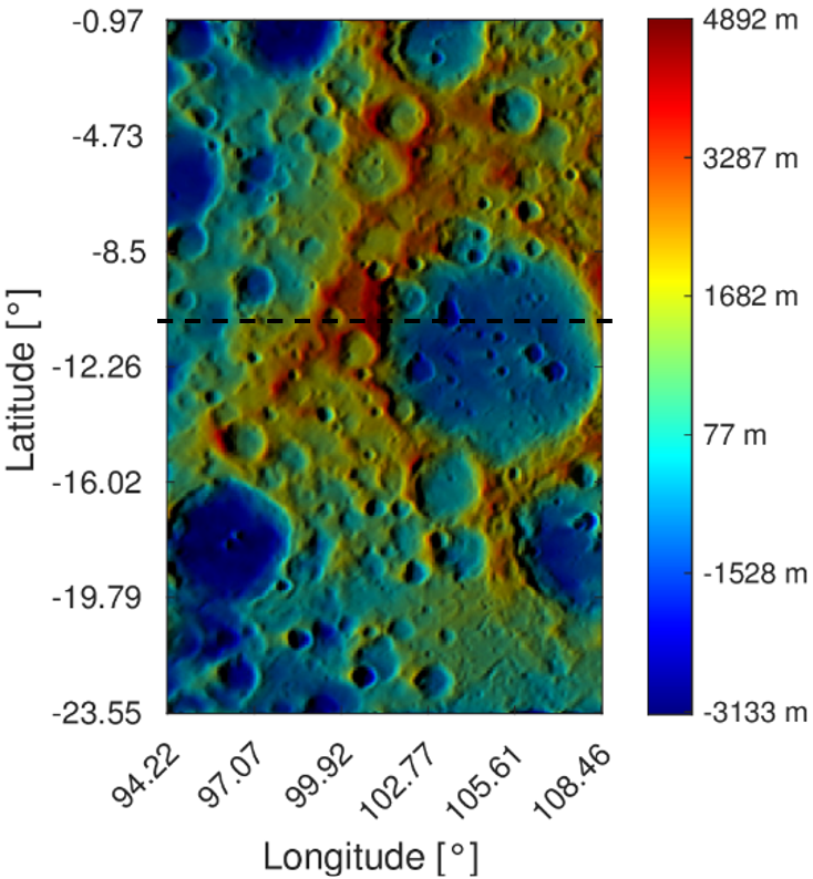
EPSC2024-247 | ECP | Posters | TP10 | OPC: evaluations required
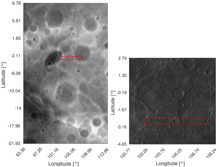
Shape and Albedo from Shading with Planetary Flyby Images of Mercury and the MoonThu, 12 Sep, 10:30–12:00 (CEST) | Poster area Level 2 – Galerie | P26
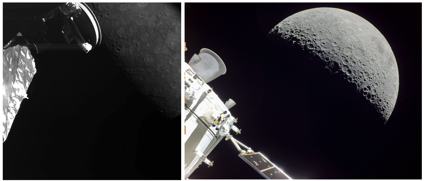 Figure 1. Left: Flyby image from the BepiColombo mission [10]. Right: Flyby image from the Artemis I mission [11].
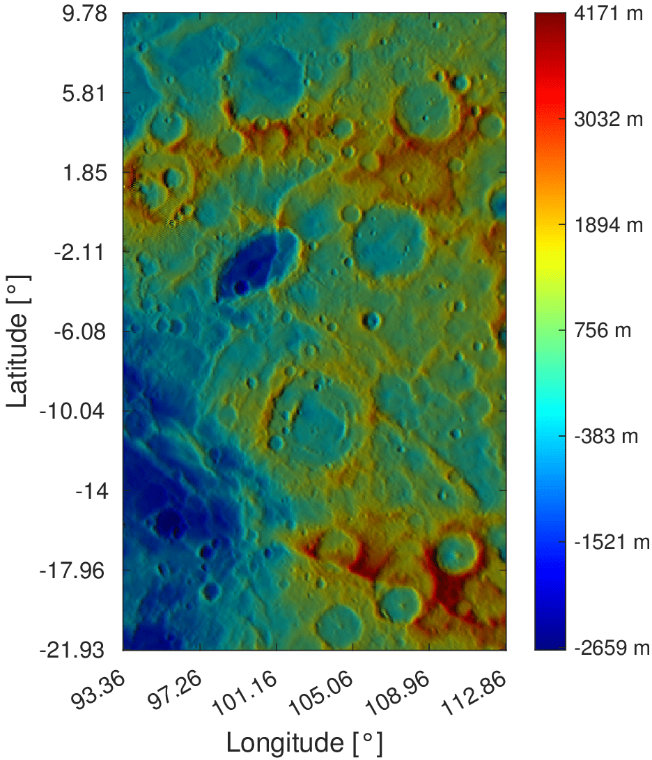

EPSC2024-646 | ECP | Posters | TP10 | OPC: evaluations required
Spectral properties of pyroclastic deposits on Mercury over space and timeThu, 12 Sep, 10:30–12:00 (CEST) | Poster area Level 2 – Galerie | P34
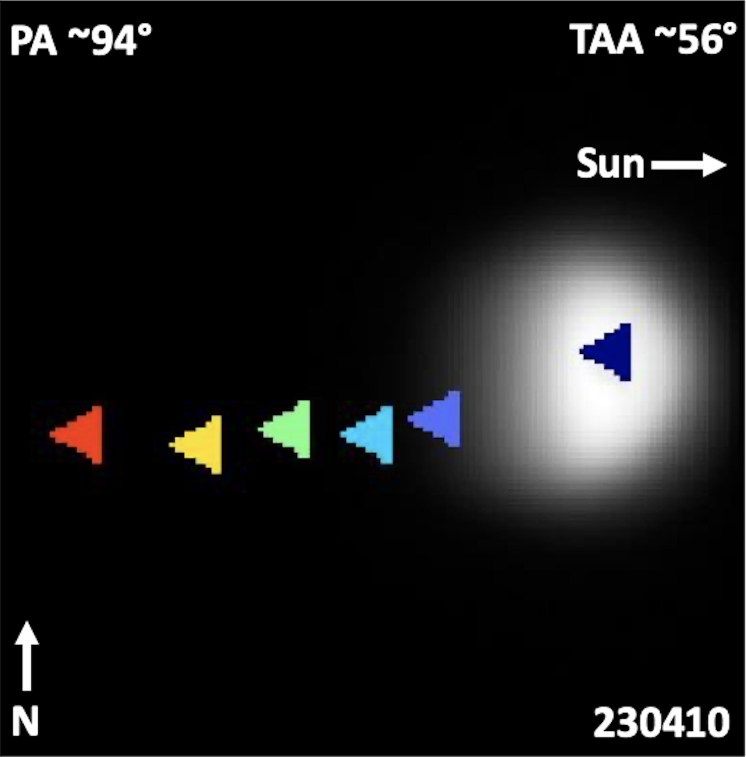
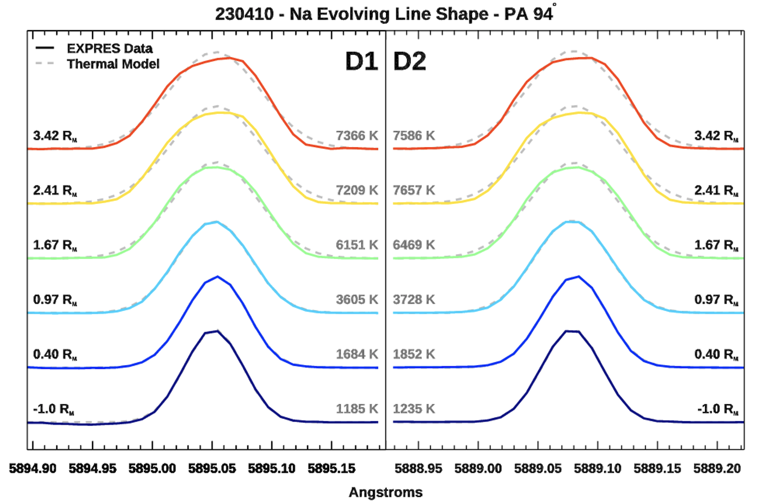
EPSC2024-757 | ECP | Posters | TP10 | OPC: evaluations required
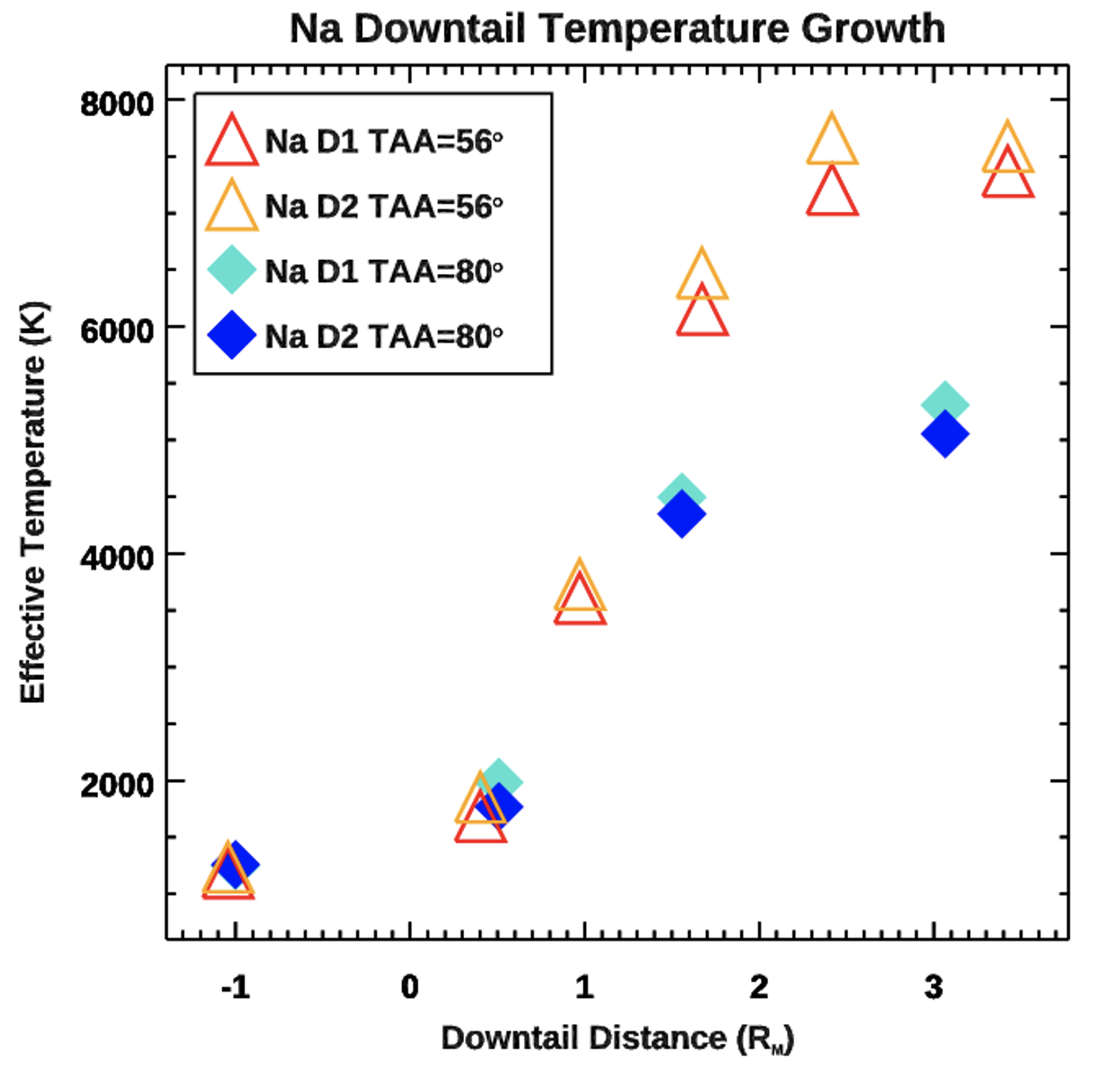
Linewidth Measurements of Mercury's Alkali ExosphereThu, 12 Sep, 10:30–12:00 (CEST) | Poster area Level 2 – Galerie | P17
EPSC2024-828 | Posters | TP10
Preliminary temperature analysis of the Region of Interest using MERTIS onboard BepiColombo for the upcoming Mercury's 5th Flyby.Thu, 12 Sep, 10:30–12:00 (CEST) | Poster area Level 2 – Galerie | P37

EPSC2024-1011 | ECP | Posters | TP10 | OPC: evaluations required
Mineralogy of the mantles in sub- Earths and exo- MercuriesThu, 12 Sep, 10:30–12:00 (CEST) | Poster area Level 2 – Galerie | P15
TP11 | Unveiling Venus from atmosphere to core
EPSC2024-836 | ECP | Posters | TP11
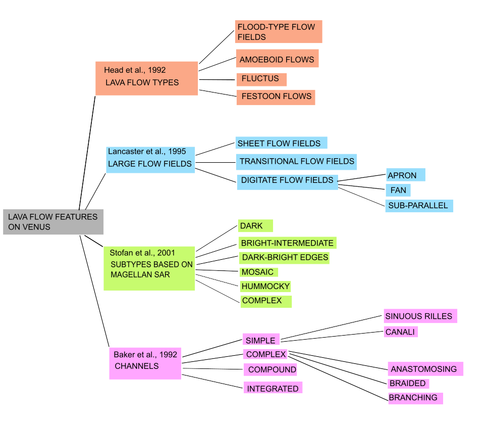
Analysis of lava flow features on Venus for radar sounder simulationsThu, 12 Sep, 10:30–12:00 (CEST) | Poster area Level 2 – Galerie | P41
EPSC2024-1042 | ECP | Posters | TP11
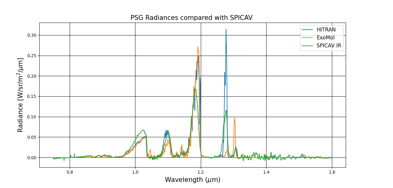
Searching for a near-surface particulate layer using near-IR spacecraft observationsThu, 12 Sep, 14:30–16:00 (CEST) | Poster area Level 2 – Galerie | P63
EPSC2024-1078 | ECP | Posters | TP11 | OPC: evaluations required
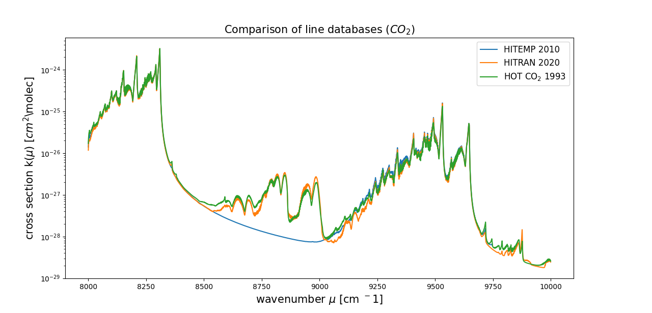
Radiative Transfer Modelling of Venus – A comparison of line databasesThu, 12 Sep, 14:30–16:00 (CEST) | Poster area Level 2 – Galerie | P64
EPSC2024-1152 | ECP | Posters | TP11
Remote Sensing Investigation of Recent Volcanic Activity on Reykjanes Peninsula, Iceland, as an Analog for VenusThu, 12 Sep, 10:30–12:00 (CEST) | Poster area Level 2 – Galerie | P46
TP12 | Lunar Science and Exploration Open Session
EPSC2024-87 | ECP | Posters | TP12 | OPC: evaluations required
In-situ extraction and purification of water on the moon – the LUWEX projectTue, 10 Sep, 14:30–16:00 (CEST) | Poster area Level 2 – Galerie | P30
EPSC2024-196 | Posters | TP12
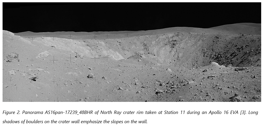
Astronaut experiences on the slopes along Apollo EVAsTue, 10 Sep, 14:30–16:00 (CEST) | Poster area Level 2 – Galerie | P45
EPSC2024-299 | ECP | Posters | TP12
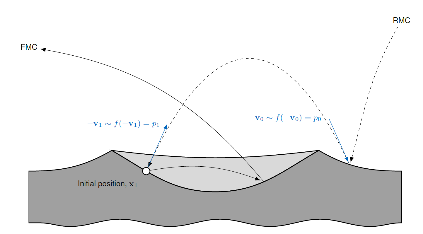
A Reverse Monte Carlo Method to Investigate the Topography Interaction with the Lunar ExosphereTue, 10 Sep, 14:30–16:00 (CEST) | Poster area Level 2 – Galerie | P32


EPSC2024-1070 | ECP | Posters | TP12 | OPC: evaluations required
Simulating the 6.5 days surface Artemis 3 mission with a first woman and man: EMMPOL20 4Artemis3 EuroMoonMarsPoland May 2024 Analog Astronaut CampaignTue, 10 Sep, 14:30–16:00 (CEST) | Poster area Level 2 – Galerie | P46
TP14 | Mars Science and Exploration
EPSC2024-877 | ECP | Posters | TP14 | OPC: evaluations required
Study of Mars mesosphere longitudinal temperature variations from NOMAD-SO onboard ESA’s TGO.Wed, 11 Sep, 10:30–12:00 (CEST) | Poster area Level 2 – Galerie | P60
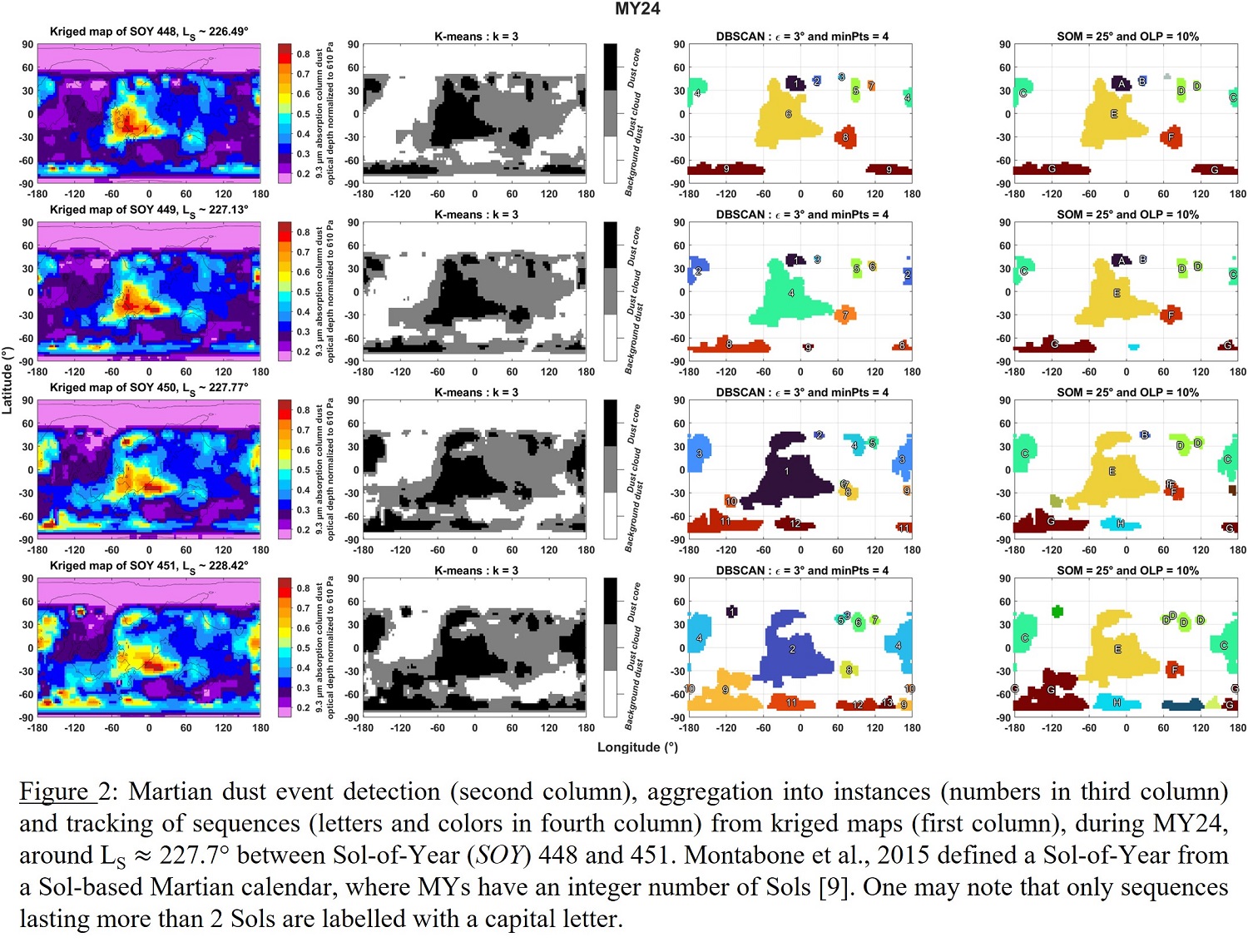
EPSC2024-1334 | ECP | Posters | TP14
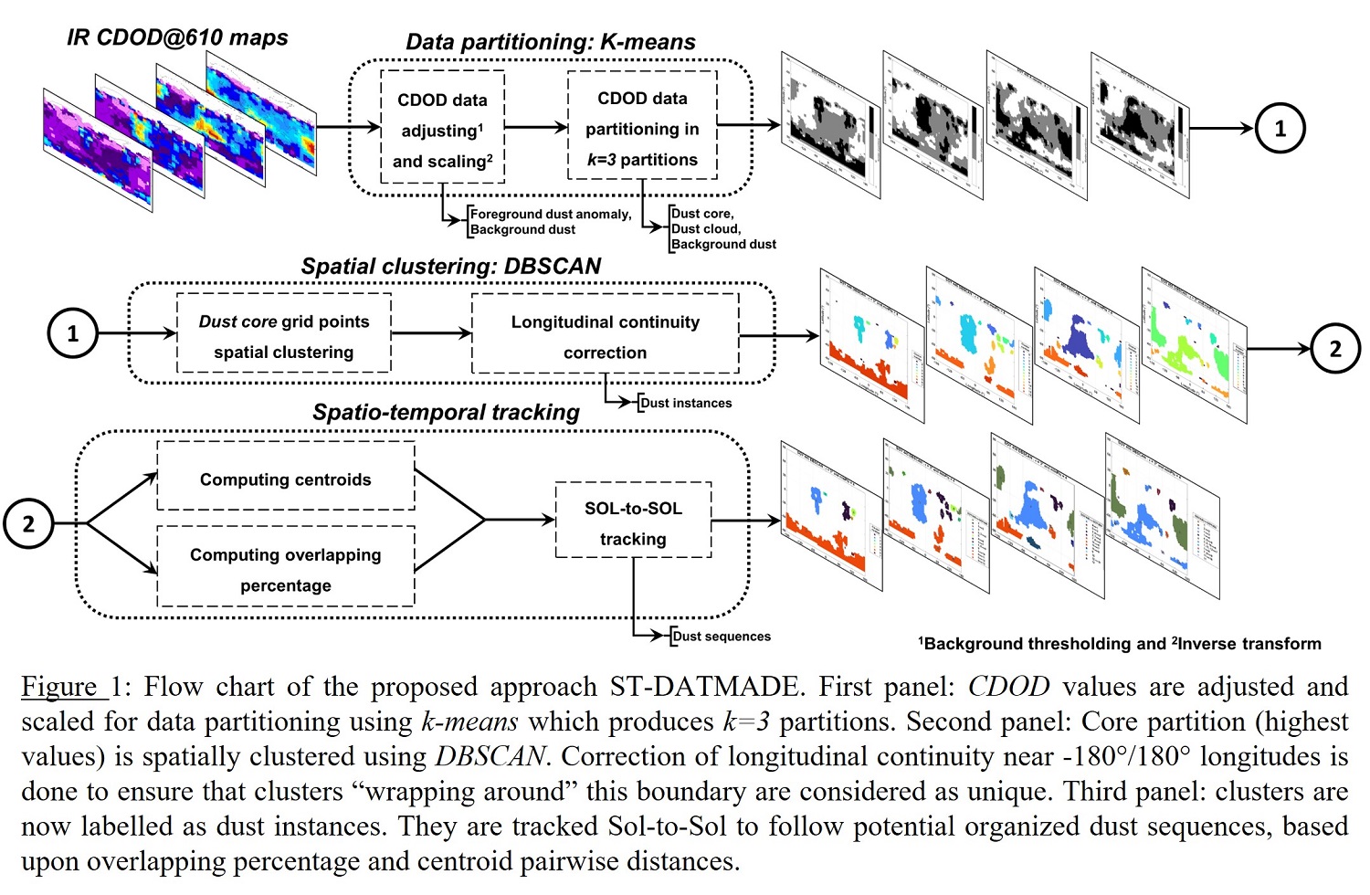
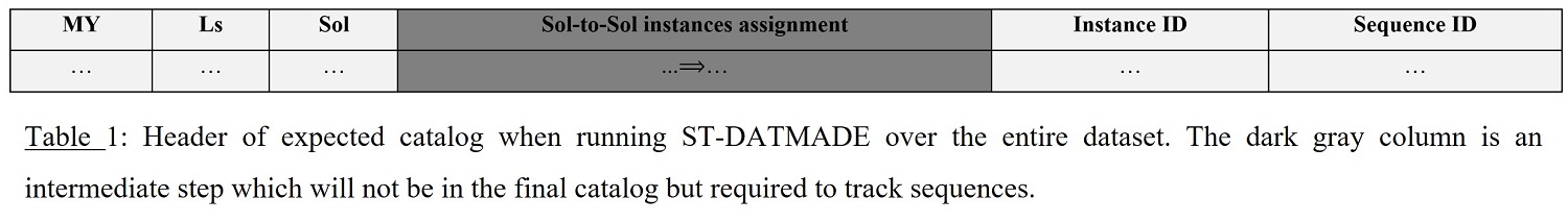
Spatio-Temporal Detection, Aggregation and Tracking of Martian Large-Scale Dust EventsWed, 11 Sep, 10:30–12:00 (CEST) | Poster area Level 2 – Galerie | P67

OPS1 | Broadening our understanding of Jupiter’s icy moons and their environment
EPSC2024-17 | Posters | OPS1 | OPC: evaluations required
Global morphology of ENA emissions from the atmosphere-magnetosphere interactions at Europa and CallistoMon, 09 Sep, 10:30–12:00 (CEST) | Poster area Level 2 – Galerie | P23
EPSC2024-75 | ECP | Posters | OPS1 | OPC: evaluations required
Non-thermal atmospheric escape of sulfur and oxygen on Io driven by photochemistry and atmospheric sputteringMon, 09 Sep, 14:30–16:00 (CEST) | Poster area Level 2 – Galerie | P31
EPSC2024-323 | ECP | Posters | OPS1 | OPC: evaluations required
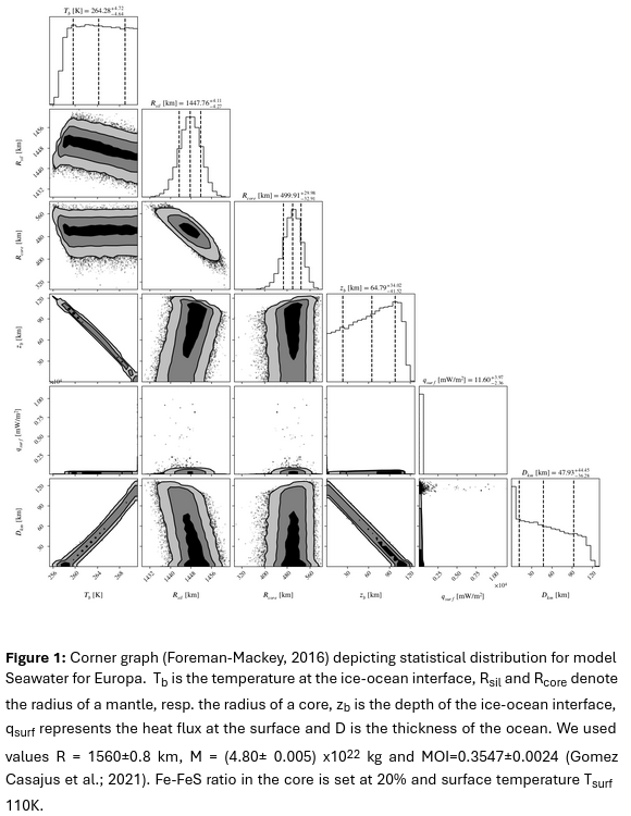
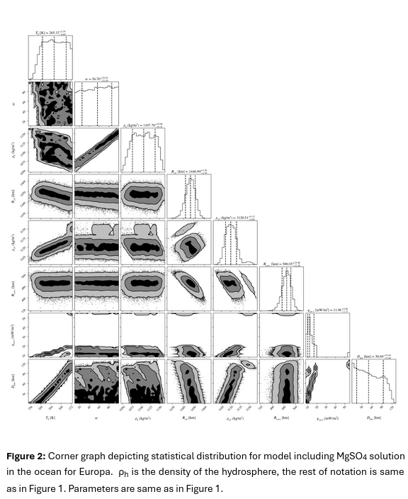
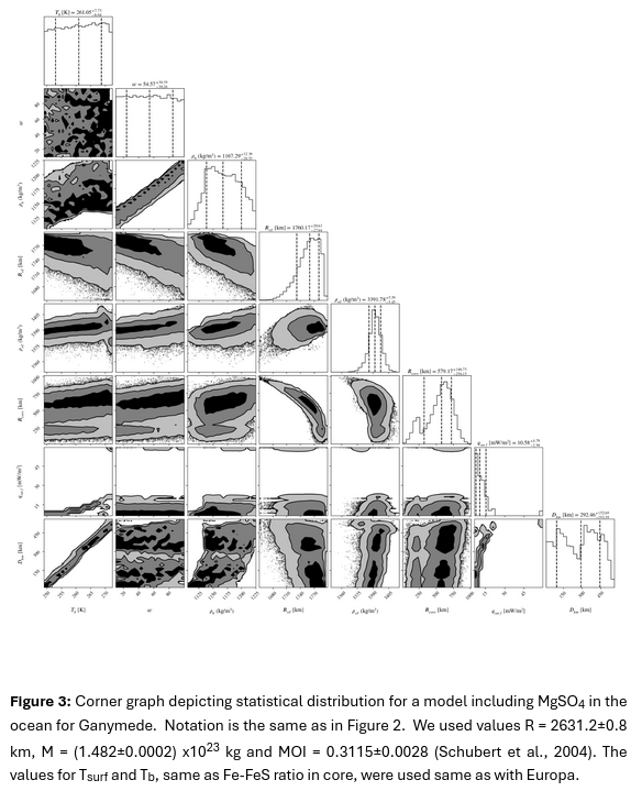
Exploring Europa and Ganymede's Internal Structure: A Statistical PerspectiveMon, 09 Sep, 14:30–16:00 (CEST) | Poster area Level 2 – Galerie | P28
EPSC2024-933 | ECP | Posters | OPS1 | OPC: evaluations required
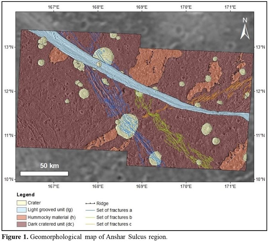
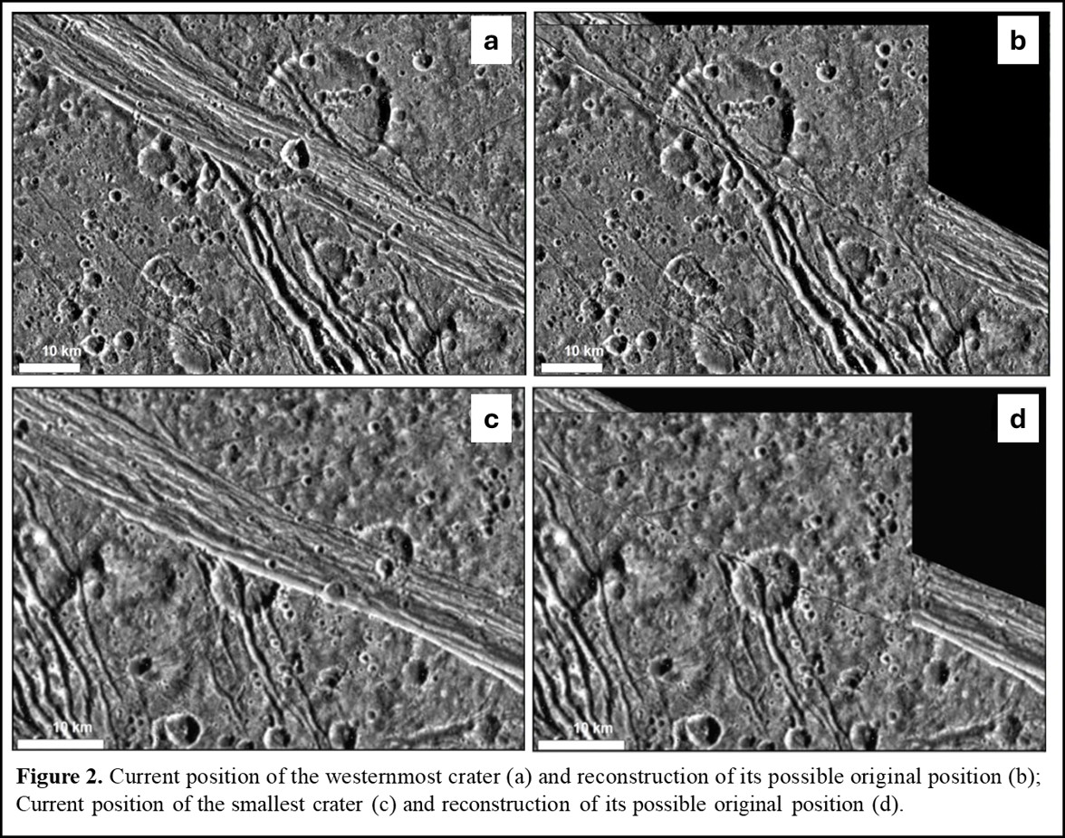
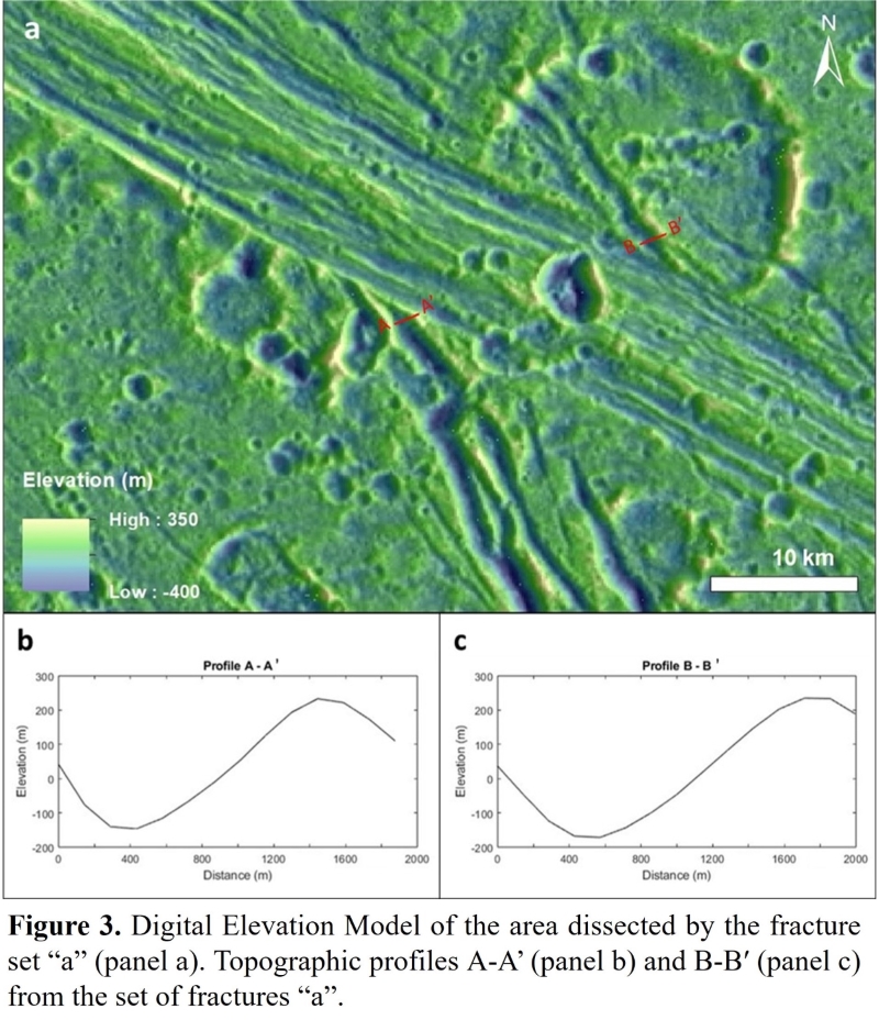
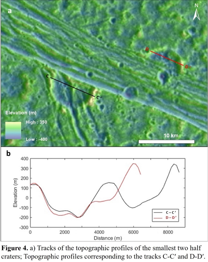
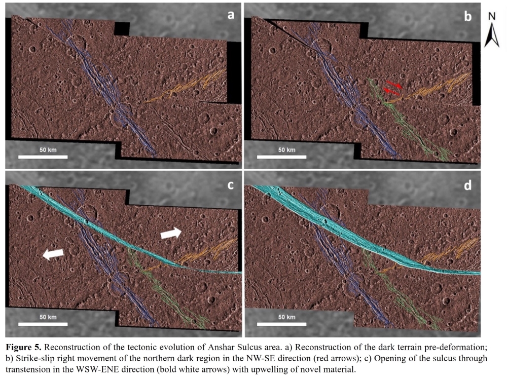
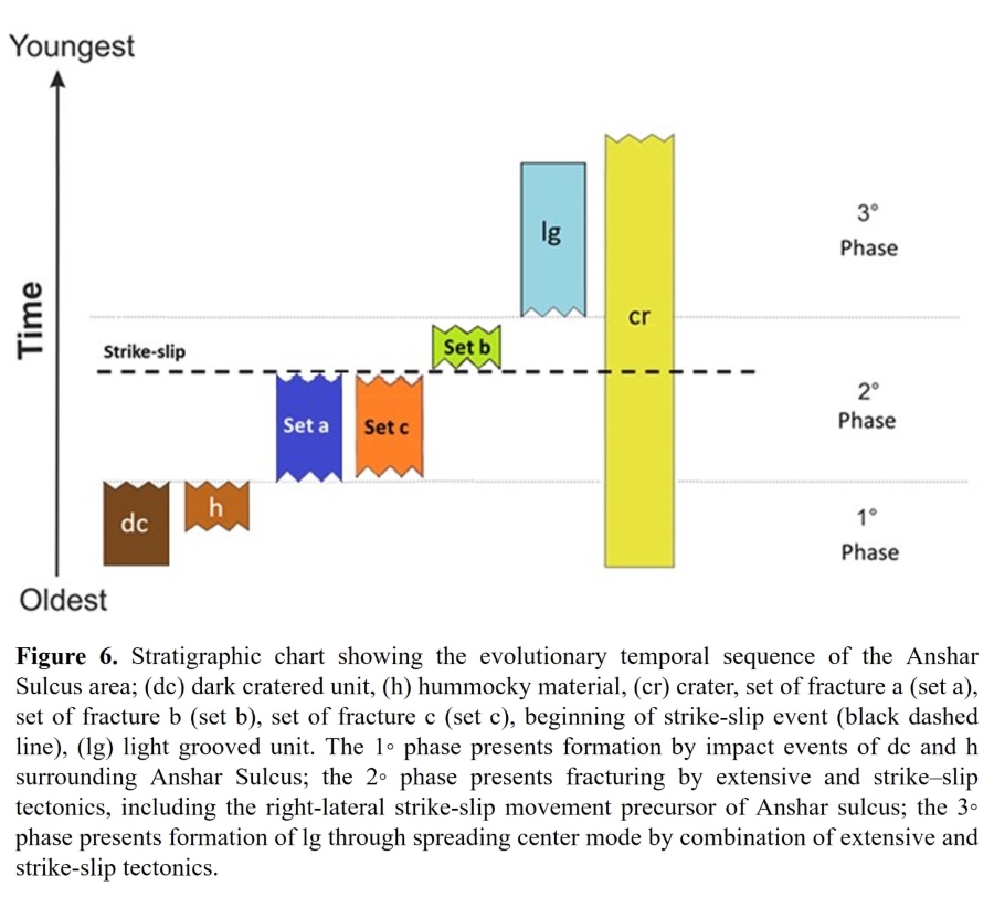
Strike-slip tectonics as a precursor to crustal spreading in Anshar Sulcus, Ganymede: Implications for grooved terrain formationMon, 09 Sep, 14:30–16:00 (CEST) | Poster area Level 2 – Galerie | P35
EPSC2024-1021 | ECP | Posters | OPS1 | OPC: evaluations required
Rayleigh-Bénard convection in the subsurface ocean of Ganymede.Mon, 09 Sep, 14:30–16:00 (CEST) | Poster area Level 2 – Galerie | P26
EPSC2024-1100 | ECP | Posters | OPS1 | OPC: evaluations required
Hiding in Plain Sight: Searching for Evidence of Subduction on Europa's Icy ShellMon, 09 Sep, 14:30–16:00 (CEST) | Poster area Level 2 – Galerie | P36
OPS2 | Jupiter and Giant Planet Systems: Juno Results
EPSC2024-496 | ECP | Posters | OPS2 | OPC: evaluations required
A long-term study of the Jovian equatorial atmosphere at the upper troposphere-lower stratosphere from HST observations in the 890-nm methane absorption bandTue, 10 Sep, 10:30–12:00 (CEST) | Poster area Level 2 – Galerie | P52
EPSC2024-669 | ECP | Posters | OPS2 | OPC: evaluations required
Latitudinal Variation in Internal Heat Flux in Jupiter's Atmosphere: Effect on Weather Layer DynamicsTue, 10 Sep, 10:30–12:00 (CEST) | Poster area Level 2 – Galerie | P53
OPS4 | The Mysterious Saturn System
EPSC2024-347 | ECP | Posters | OPS4 | OPC: evaluations required
Pick-up ion distributions in the inner and middle Saturnian MagnetosphereWed, 11 Sep, 14:30–16:00 (CEST) | Poster area Level 2 – Galerie | P69
OPS5 | Exploration of Titan
EPSC2024-226 | Posters | OPS5 | OPC: evaluations required
On the evolution of the primordial hydrosphere of TitanTue, 10 Sep, 14:30–16:00 (CEST) | Poster area Level 2 – Galerie | P69
EPSC2024-428 | ECP | Posters | OPS5 | OPC: evaluations required
Seasonal variation of Titan’s stratospheric tiltTue, 10 Sep, 14:30–16:00 (CEST) | Poster area Level 2 – Galerie | P65
OPS7 | Aerosols and clouds in planetary atmospheres
EPSC2024-294 | ECP | Posters | OPS7 | OPC: evaluations required
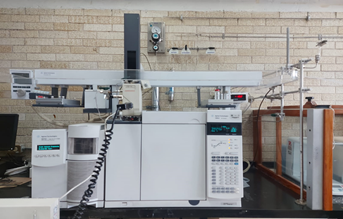
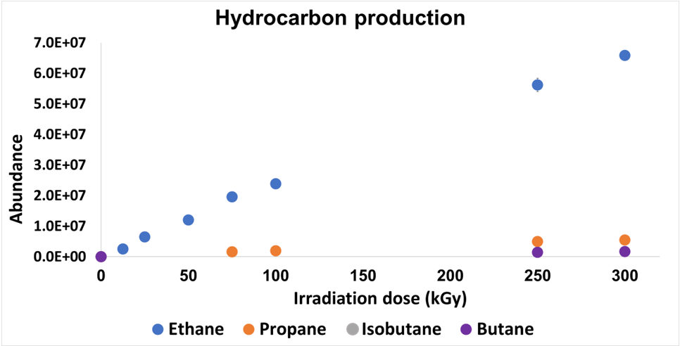
Study of the incidence of gamma radiation on a simulated atmosphere of Titan: An experimental approachMon, 09 Sep, 10:30–12:00 (CEST) | Poster area Level 2 – Galerie | P41


EPSC2024-429 | Posters | OPS7 | OPC: evaluations required
One-dimensional Microphysics Model of Venusian Clouds from 40 to 100 km: Impact of the Middle-atmosphere Eddy Transport and SOIR Temperature Profile on the Cloud StructureMon, 09 Sep, 10:30–12:00 (CEST) | Poster area Level 2 – Galerie | P37
MITM1 | Planetary Missions, Instrumentations, and mission concepts: new opportunities for planetary exploration
EPSC2024-707 | ECP | Posters | MITM1
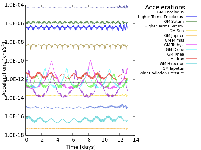
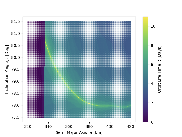
Numerical analysis of polar orbits for future Enceladus missionsMon, 09 Sep, 14:30–16:00 (CEST) | Poster area Level 2 – Galerie | P54
EPSC2024-881 | ECP | Posters | MITM1 | OPC: evaluations required
CHirality Analyzer In-Situ (CHAIS) - A Novel Approach to Planetary Surface CharacterisationMon, 09 Sep, 14:30–16:00 (CEST) | Poster area Level 2 – Galerie | P60

MITM3 | Artificial Intelligence and Machine Learning in Planetary Science
EPSC2024-318 | ECP | Posters | MITM3 | OPC: evaluations required
Artificial intelligence at the service of space astrometry: a new way to explore the solar systemTue, 10 Sep, 10:30–12:00 (CEST) | Poster area Level 1 – Intermezzo | I1
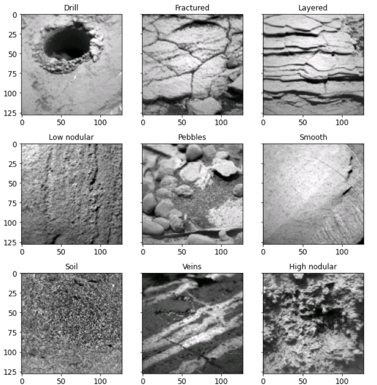
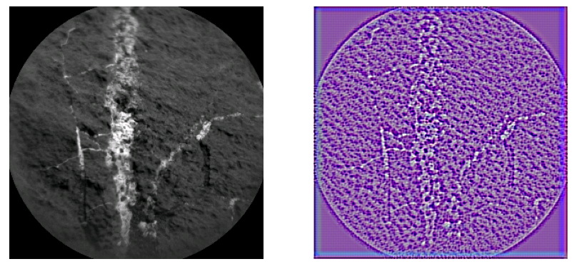
EPSC2024-780 | Posters | MITM3 | OPC: evaluations required
ChemCam rock classification using explainable AITue, 10 Sep, 10:30–12:00 (CEST) | Poster area Level 1 – Intermezzo | I8
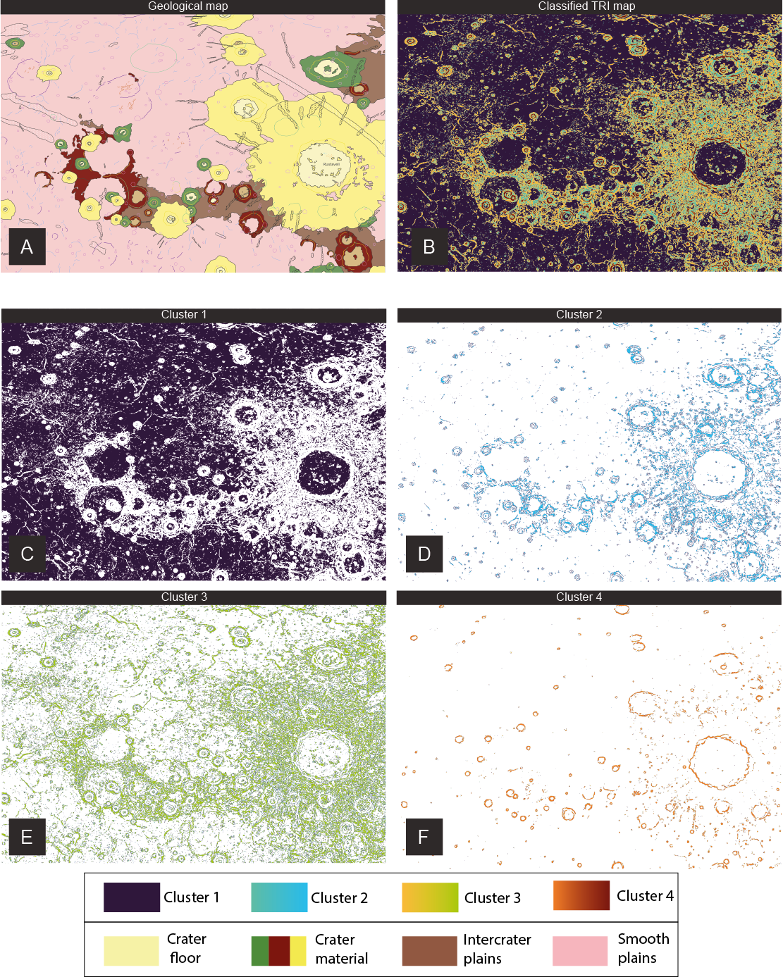
EPSC2024-934 | ECP | Posters | MITM3 | OPC: evaluations required
Unsupervised classification of Mercury’s surface to aid the reconstruction of explorative geological maps.Tue, 10 Sep, 10:30–12:00 (CEST) | Poster area Level 1 – Intermezzo | I6
MITM5 | In-situ planetary measurements
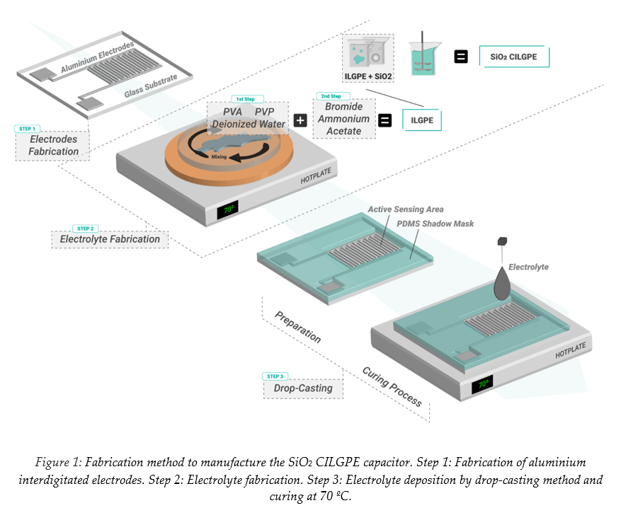
EPSC2024-936 | ECP | Posters | MITM5
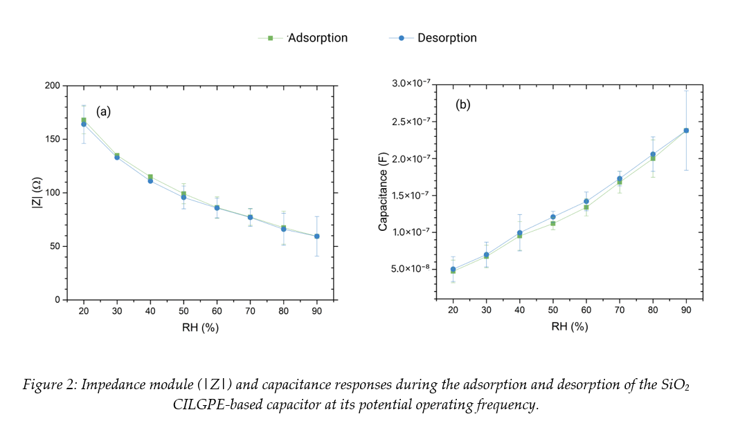
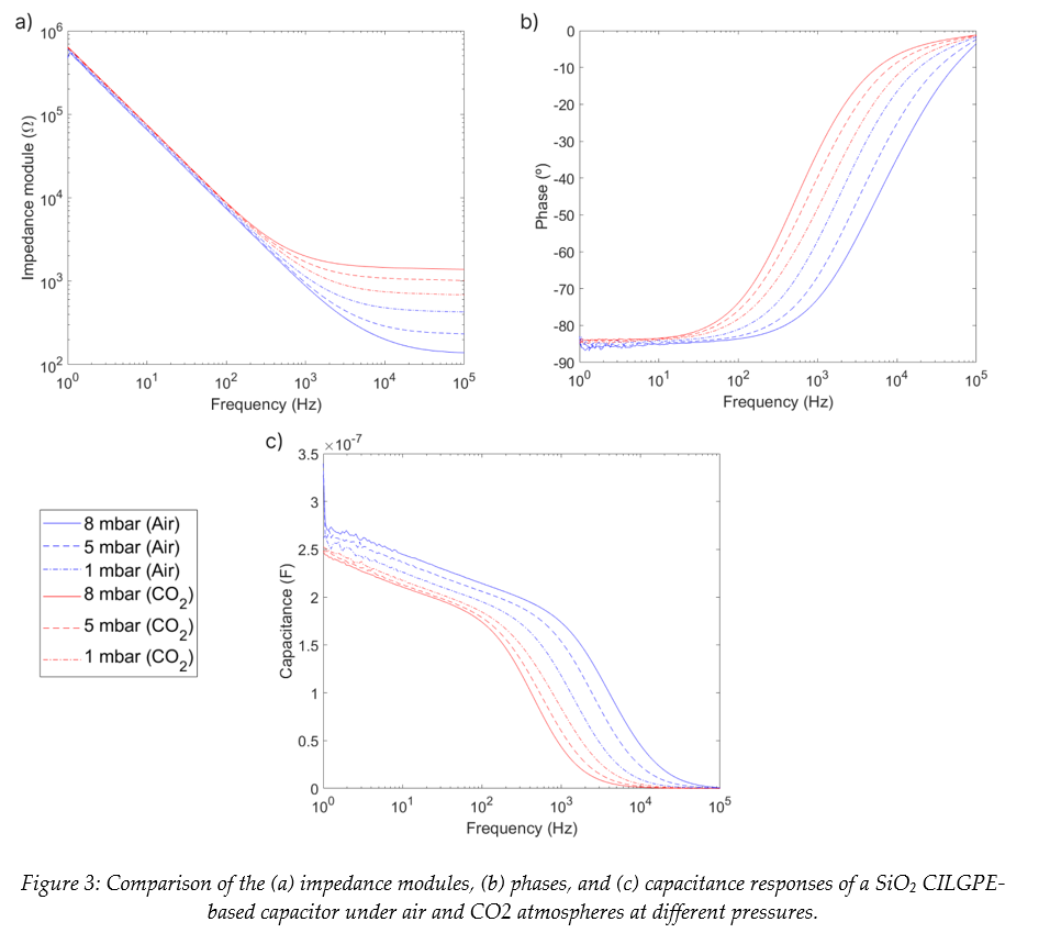
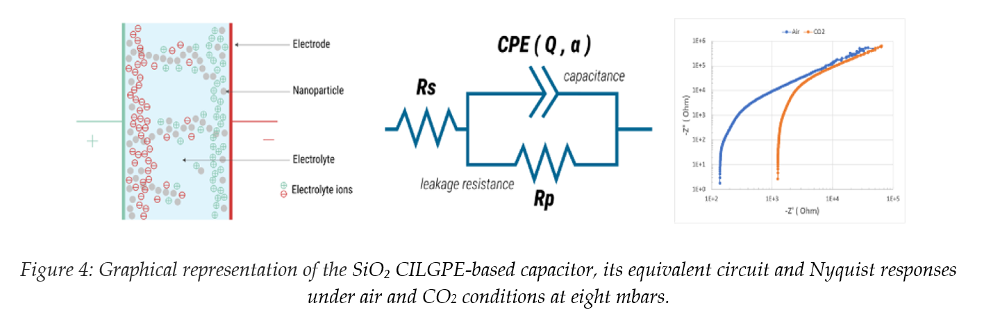
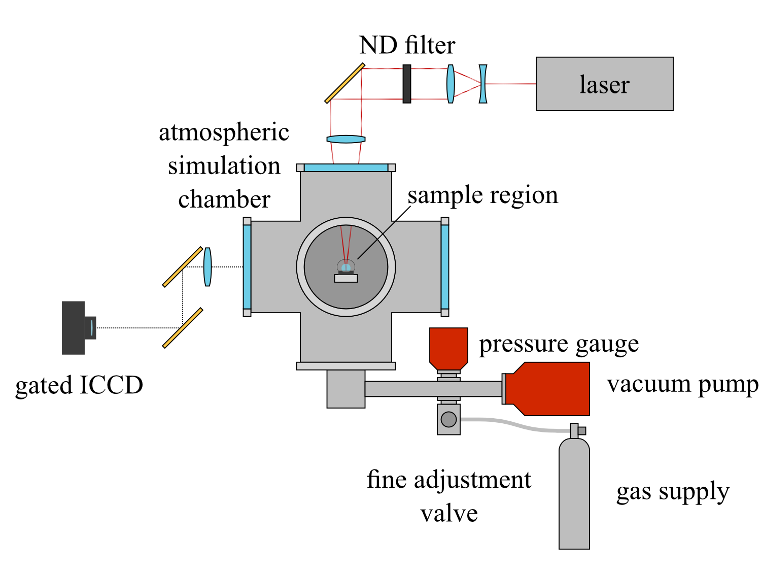
Electrochemical impedance spectroscopy analysis of a SiO2 submicron-particles-based relative humidity sensor for planetary research applicationsFri, 13 Sep, 14:30–16:00 (CEST) | Poster area Level 1 – Intermezzo | I24
MITM6 | Laboratory experiments in support of ground observations and space missions (sample return, analogs, analytical workflow etc.).
EPSC2024-232 | Posters | MITM6 | OPC: evaluations required
Evolution of Laser-Induced Plasmas for In-Situ Analysis on Planetary BodiesThu, 12 Sep, 14:30–16:00 (CEST) | Poster area Level 1 – Intermezzo | I9
EPSC2024-867 | ECP | Posters | MITM6
Laboratory hyperspectral analysis of icy mixtures with Martian SimulantsThu, 12 Sep, 14:30–16:00 (CEST) | Poster area Level 1 – Intermezzo | I4
EPSC2024-1299 | ECP | Posters | MITM6 | OPC: evaluations required
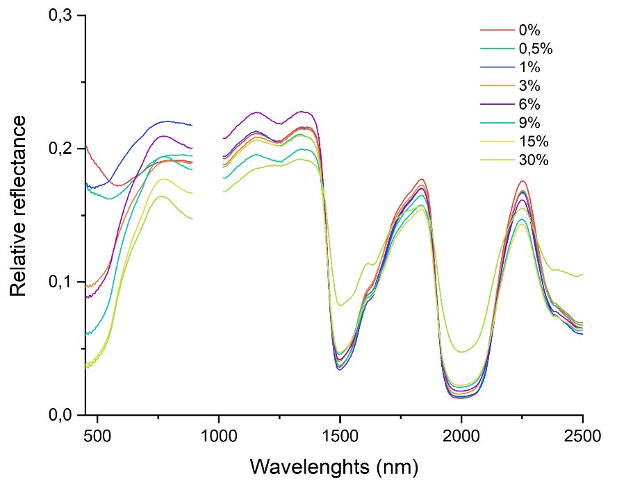
Dimensionality reduction on MIR spectra of powdered silicate glasses as analogues for volcanic ashesThu, 12 Sep, 14:30–16:00 (CEST) | Poster area Level 1 – Intermezzo | I14
MITM8 | Future and current instruments to detect and characterise extrasolar planets and their environment
EPSC2024-620 | ECP | Posters | MITM8
EXODUS: A mission to explore exoplanet evolution through understanding atmospheric escapeThu, 12 Sep, 10:30–12:00 (CEST) | Poster area Level 1 – Intermezzo | I22
EPSC2024-1202 | ECP | Posters | MITM8 | OPC: evaluations required
Designing new Stellar Activity Metrics for use with Exoplanet Transmission Spectra Obtained with both Current and Future MissionsThu, 12 Sep, 10:30–12:00 (CEST) | Poster area Level 1 – Intermezzo | I24
SB2 | Beyond the Surveys: Observations, Modelling and Follow-up of Asteroids from Ground
EPSC2024-188 | ECP | Posters | SB2 | OPC: evaluations required
Analysis of photocentre offset from Gaia astrometry on selected asteroids and planetary satellitesMon, 09 Sep, 14:30–16:00 (CEST) | Poster area Level 1 – Intermezzo | I3
EPSC2024-640 | ECP | Posters | SB2 | OPC: evaluations required
AsteroiDB: The Asteroid Legacy Archive of the Canary Islands ObservatoriesMon, 09 Sep, 14:30–16:00 (CEST) | Poster area Level 1 – Intermezzo | I15
EPSC2024-1143 | ECP | Posters | SB2
Thermophysical Modeling and Parameter Estimation for 3375 AsteroidsMon, 09 Sep, 14:30–16:00 (CEST) | Poster area Level 1 – Intermezzo | I12
SB3 | Small Body Surfaces: Windows into Geological Space and Time
EPSC2024-566 | ECP | Posters | SB3
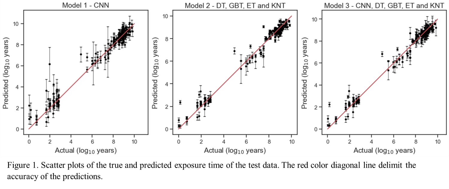
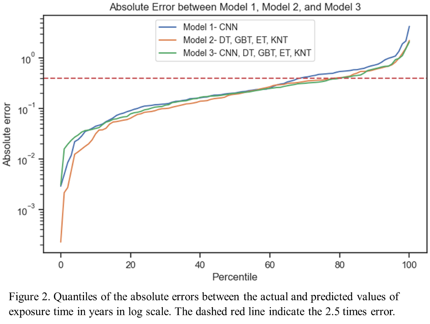
Predicting the surface exposure time of asteroids using the space weathering features in reflectance spectra: small data machine learning.Wed, 11 Sep, 14:30–16:00 (CEST) | Poster area Level 1 – Intermezzo | I7
EPSC2024-617 | ECP | Posters | SB3 | OPC: evaluations required
Radiance Morphological Mapping for Small Body Surface InvestigationsWed, 11 Sep, 14:30–16:00 (CEST) | Poster area Level 1 – Intermezzo | I4
SB6 | Surface and interiors of small bodies, meteorite parent bodies, and icy moons: thermal properties, evolution, and structure
EPSC2024-467 | ECP | Posters | SB6
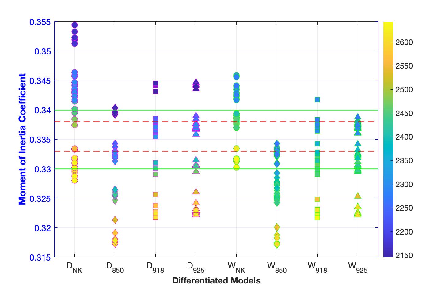
Exploring Enceladus: Internal Structure Models and Moment of InertiaMon, 09 Sep, 10:30–12:00 (CEST) | Poster area Level 1 – Intermezzo | I17
EPSC2024-499 | ECP | Posters | SB6 | OPC: evaluations required
Experimental results from the CoPhyLab -Detection of the influences of surface structureson particle ejection in comet-simulationexperimentsMon, 09 Sep, 10:30–12:00 (CEST) | Poster area Level 1 – Intermezzo | I24

EPSC2024-557 | ECP | Posters | SB6 | OPC: evaluations required
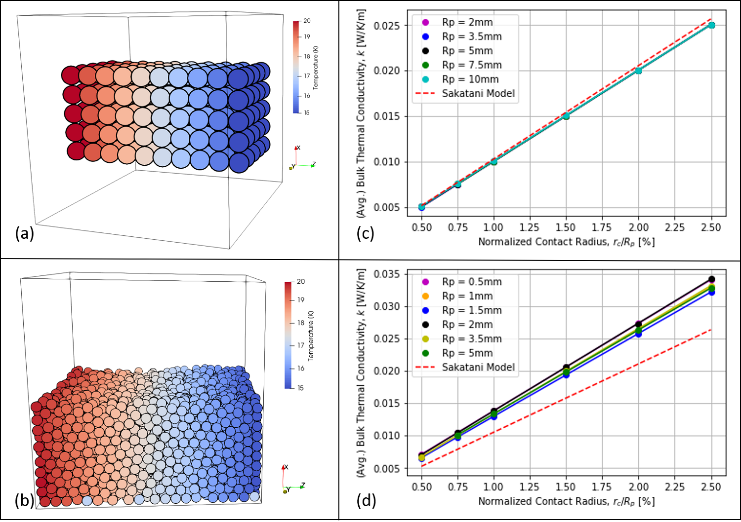
A numerical method to determine bulk thermal conductivity of randomly packed particle bedsMon, 09 Sep, 10:30–12:00 (CEST) | Poster area Level 1 – Intermezzo | I26
EPSC2024-614 | ECP | Posters | SB6 | OPC: evaluations required
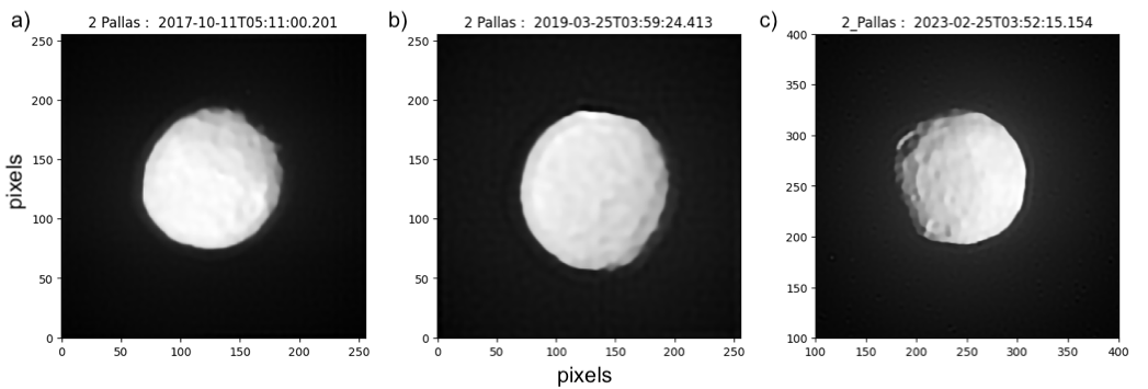
Asteroid (2) Pallas: a trip from the limbs profiles to the interiorMon, 09 Sep, 10:30–12:00 (CEST) | Poster area Level 1 – Intermezzo | I18
SB12 | Centaurs and Trans-Neptunian objects
EPSC2024-472 | ECP | Posters | SB12 | OPC: evaluations required
Analysis of a double star occultation by TNO (470316) 2007 OC10Tue, 10 Sep, 14:30–16:00 (CEST) | Poster area Level 1 – Intermezzo | I22
SB13 | Icy Ocean Worlds, Comets and Asteroids in the Laboratory
EPSC2024-973 | ECP | Posters | SB13
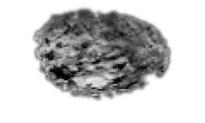
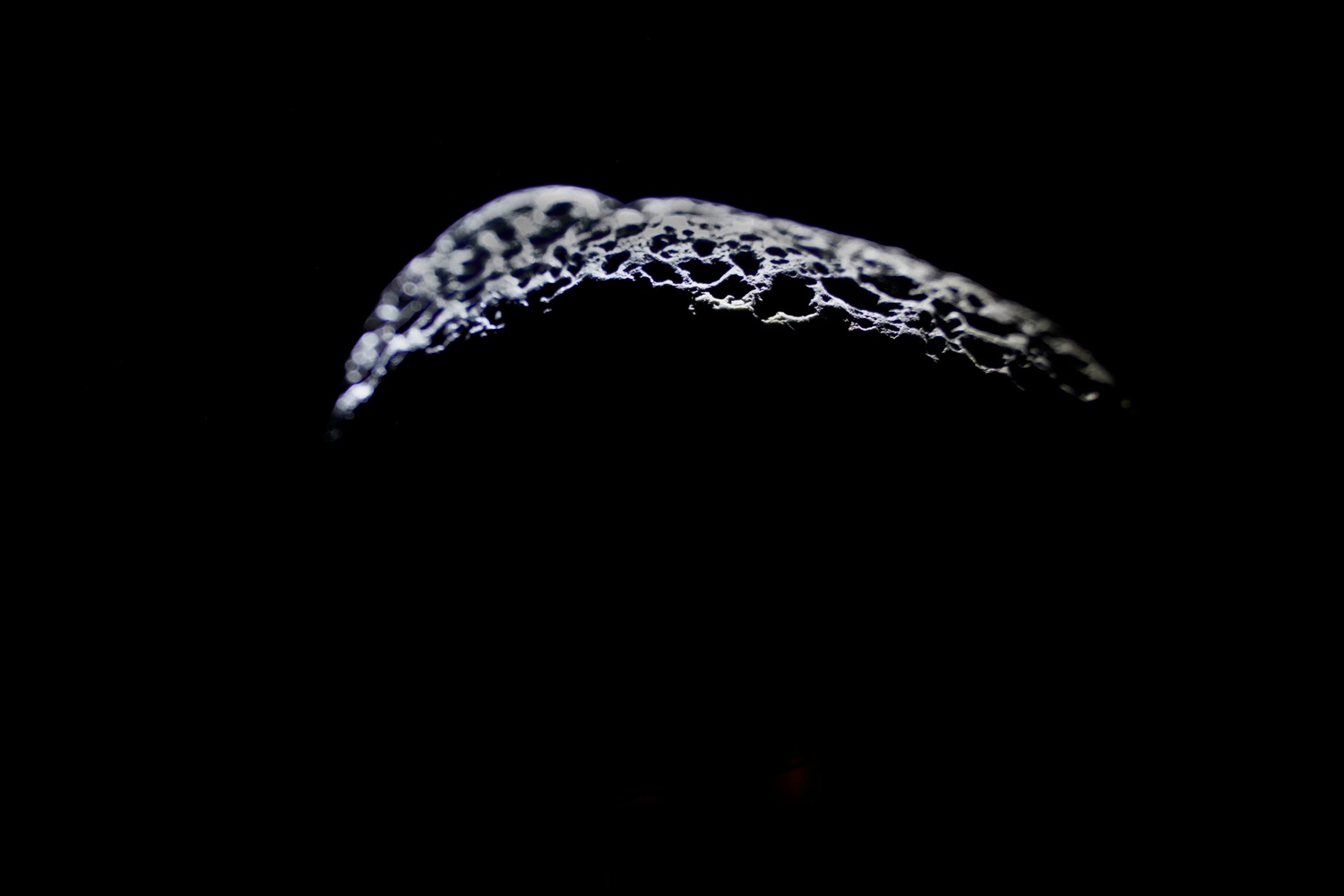
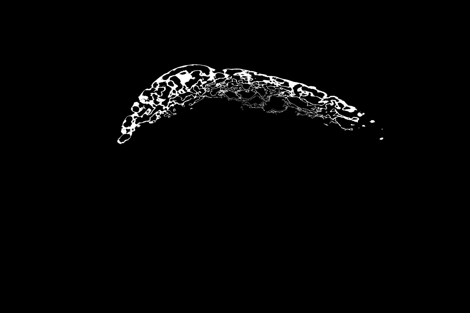
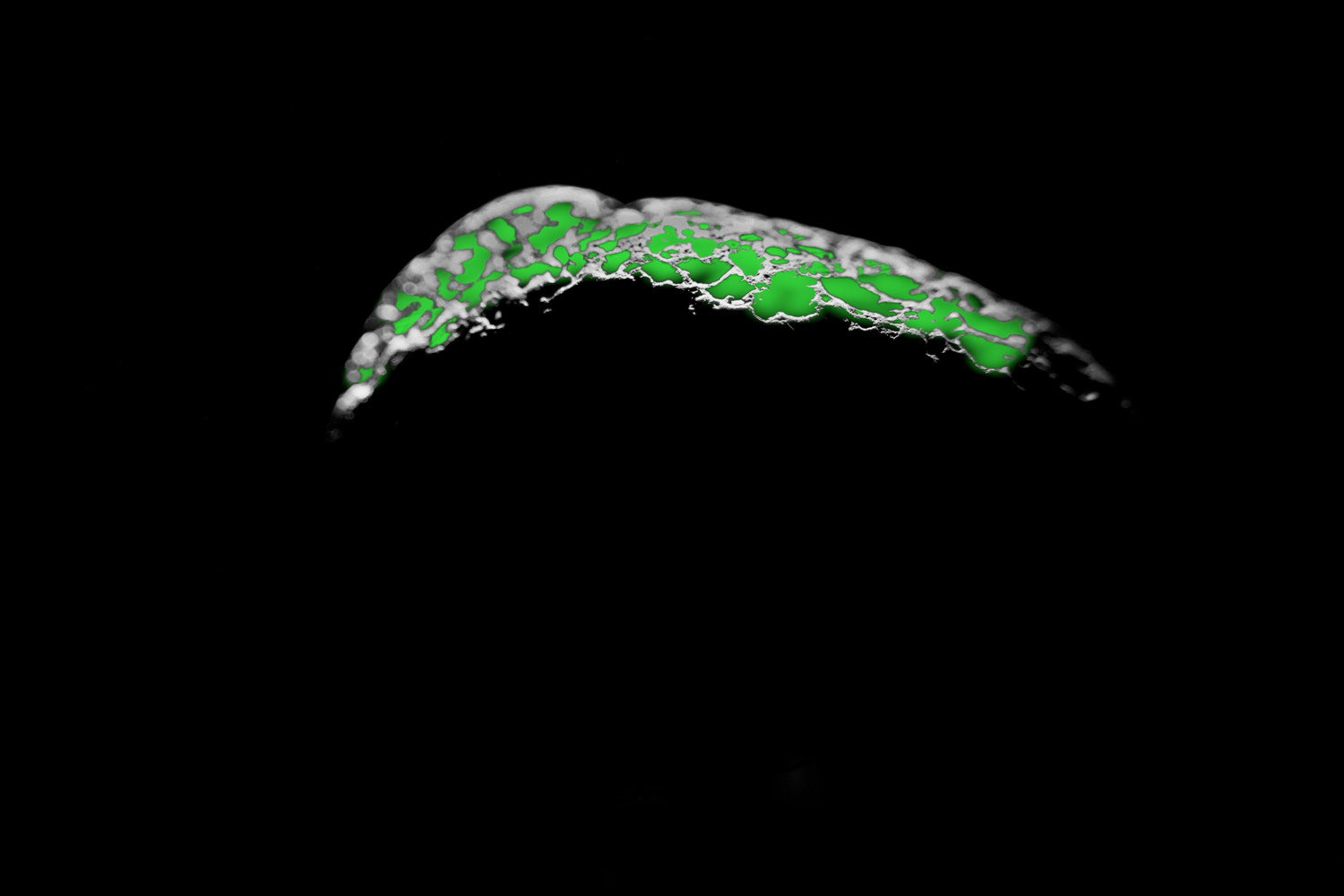
Growing a putative inhabitant of Enceladus’ ocean surfaceThu, 12 Sep, 10:30–12:00 (CEST) | Poster area Level 1 – Intermezzo | I35
EPSC2024-1081 | Posters | SB13 | OPC: evaluations required
Detecting cellular biosignatures from single salt-rich ice grains emitted from Enceladus or EuropaThu, 12 Sep, 10:30–12:00 (CEST) | Poster area Level 1 – Intermezzo | I36
EPSC2024-1314 | ECP | Posters | SB13
Measuring Exsolution Rates of Gases in a Laboratory Analog for Enceladus Plume FormationThu, 12 Sep, 10:30–12:00 (CEST) | Poster area Level 1 – Intermezzo | I38
EXOA1 | Towards a better understanding of planets' and planetary systems' diversity
EPSC2024-649 | ECP | Posters | EXOA1 | OPC: evaluations required
Reflectance and Emission Modelling of Airless ExoplanetsMon, 09 Sep, 14:30–16:00 (CEST) | Poster area Level 1 – Intermezzo | I38
EPSC2024-908 | ECP | Posters | EXOA1 | OPC: evaluations required
Confirmation of the long-period Exoplanet TOI-4409 bMon, 09 Sep, 14:30–16:00 (CEST) | Poster area Level 1 – Intermezzo | I36


EXOA2 | Characterizing the diversity of exoplanetary atmospheres
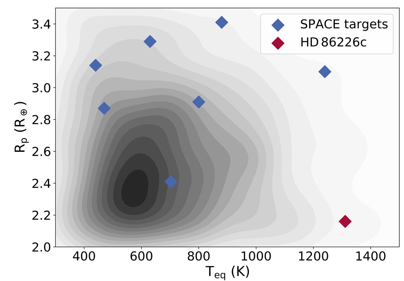
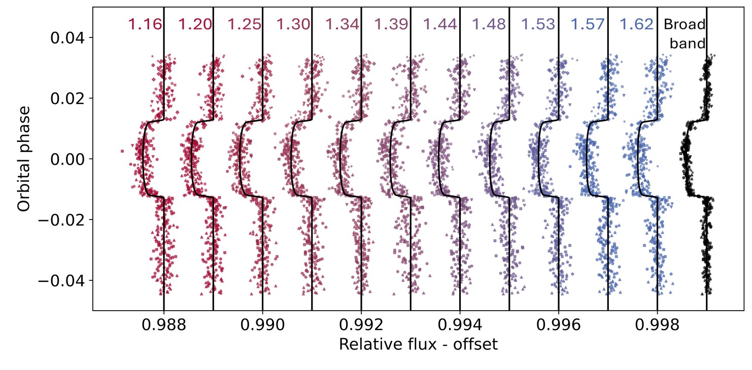
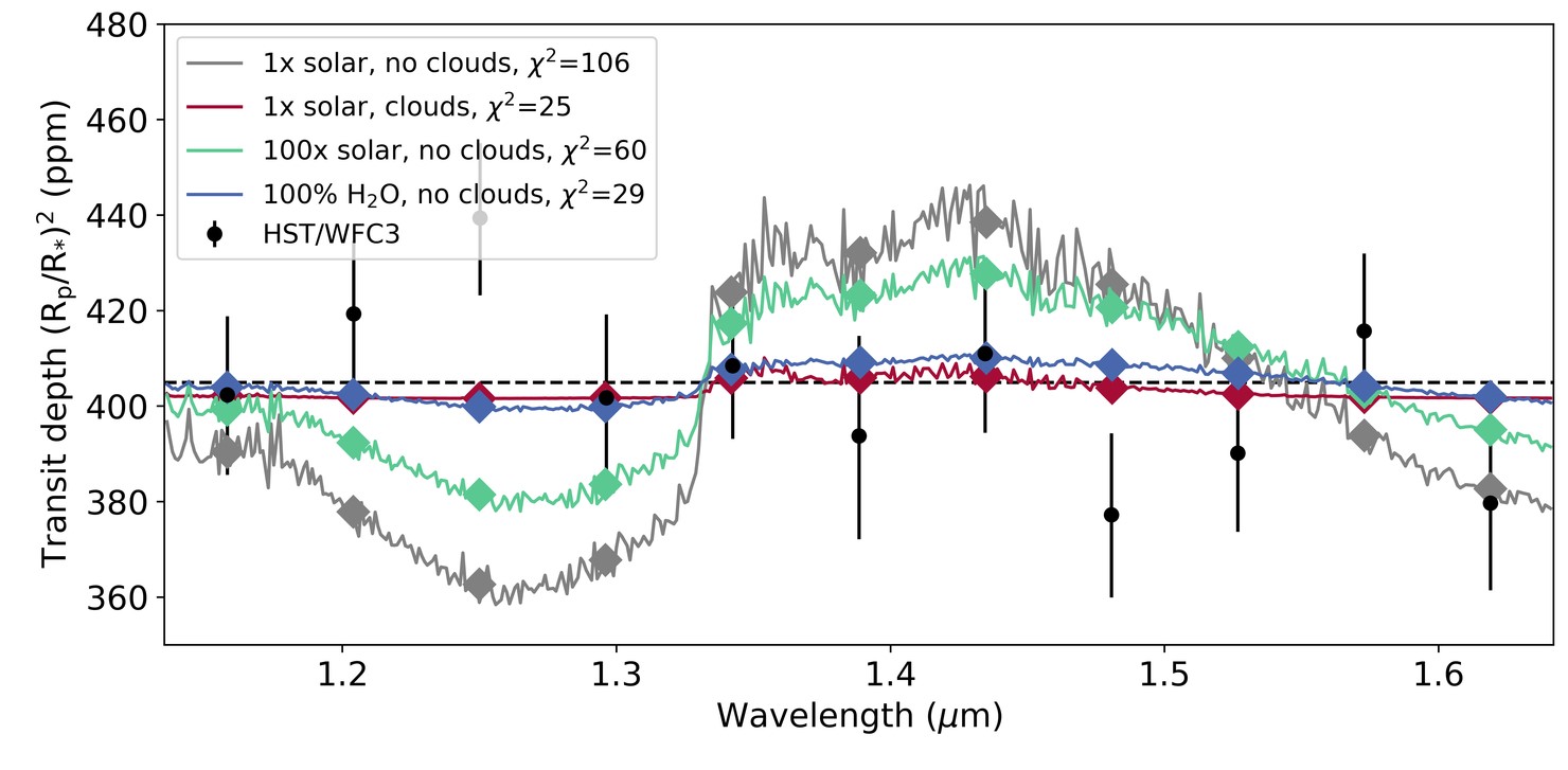
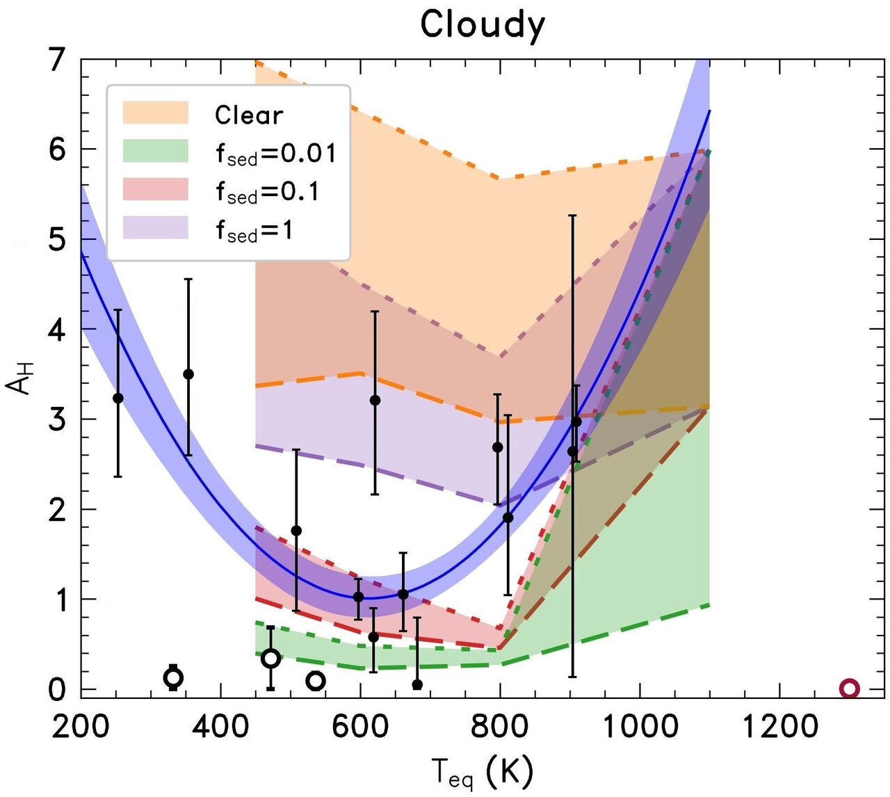
EPSC2024-627 | ECP | Posters | EXOA2
First results of the SPACE Program: The surprisingly featureless spectrum of hot sub-Neptune HD 86226cWed, 11 Sep, 14:30–16:00 (CEST) | Poster area Level 1 – Intermezzo | I10
EPSC2024-1102 | ECP | Posters | EXOA2
Convective mixing in giant planets: When does the atmospheric composition represent the planetary bulk composition?Wed, 11 Sep, 14:30–16:00 (CEST) | Poster area Level 1 – Intermezzo | I12
EXOA3 | Molecular complexity in space: from the interstellar medium to the Solar System
EPSC2024-1035 | ECP | Posters | EXOA3 | OPC: evaluations required
Unveiling the Si+ chemistry in the Interstellar Medium: an ionic reaction pathway to SiSWed, 11 Sep, 10:30–12:00 (CEST) | Poster area Level 1 – Intermezzo | I15
EXOA4 | Astrobiology and Origins
EPSC2024-12 | ECP | Posters | EXOA4
A novel metric for assessing planetary surface habitabilityWed, 11 Sep, 10:30–12:00 (CEST) | Poster area Level 1 – Intermezzo | I24
EPSC2024-469 | ECP | Posters | EXOA4
Estimating detectability of phosphine in the Venusian atmosphere using spectral modelingWed, 11 Sep, 10:30–12:00 (CEST) | Poster area Level 1 – Intermezzo | I21
EPSC2024-1150 | ECP | Posters | EXOA4 | OPC: evaluations required
Survival of microorganisms in Europa-relevant brines and conditionsWed, 11 Sep, 10:30–12:00 (CEST) | Poster area Level 1 – Intermezzo | I19
EXOA5 | Mineral surfaces in the origin and detection of Life on Earth and beyond
EPSC2024-253 | ECP | Posters | EXOA5 | OPC: evaluations required
Pellet-grown chemical gardens in horizontal planar confined geometry : Diffusion-controlled growth and osmotic fractureThu, 12 Sep, 10:30–12:00 (CEST) | Poster area Level 2 – Galerie | P75
EXOA6 | Planetary Atmospheres: a key to the evolution of planets
EPSC2024-209 | Posters | EXOA6 | OPC: evaluations required
Atmospheric compositional variations due to changes in mantle redox stateTue, 10 Sep, 10:30–12:00 (CEST) | Poster area Level 1 – Intermezzo | I33
EPSC2024-1014 | ECP | Posters | EXOA6 | OPC: evaluations required
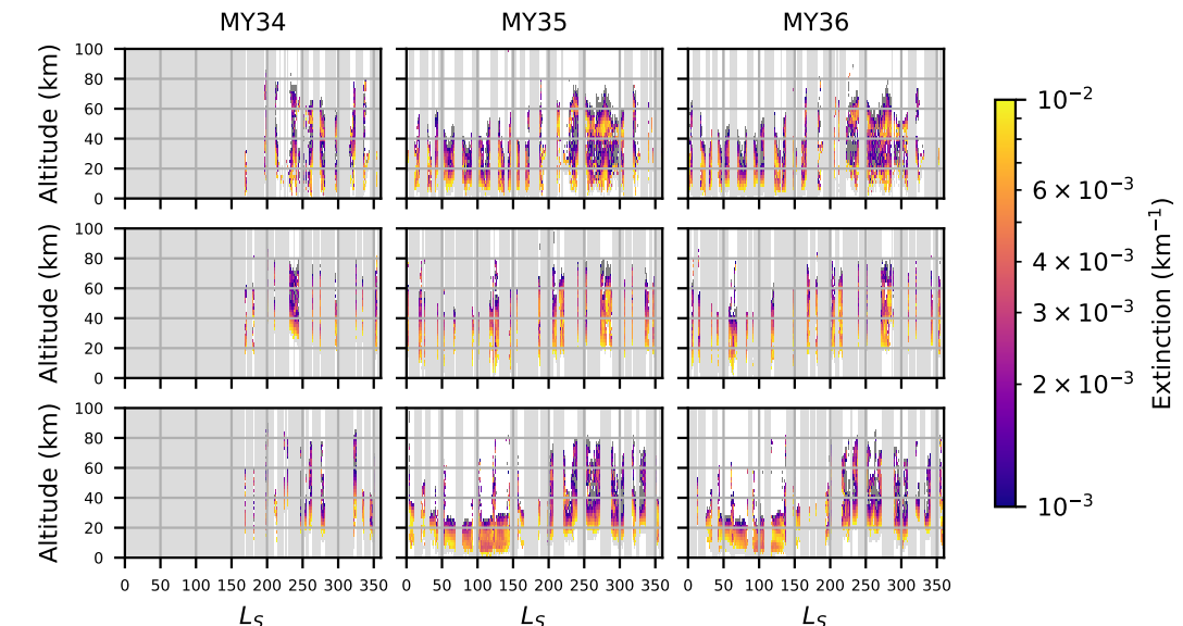
Aerosol Climatology on Mars as Observed by NOMAD UVIS/SO on ExoMars TGOTue, 10 Sep, 10:30–12:00 (CEST) | Poster area Level 1 – Intermezzo | I31

EXOA8 | Exoplanet characterization of (super-)Earths and sub-Neptunes
EPSC2024-1017 | ECP | Posters | EXOA8 | OPC: evaluations required
The influence of external factors on surface regimes of terrestrial planetsFri, 13 Sep, 14:30–16:00 (CEST) | Poster area Level 2 – Galerie | P46
EPSC2024-1088 | ECP | Posters | EXOA8 | OPC: evaluations required
Advancing Exoplanet Transit Characterization through Machine LearningFri, 13 Sep, 14:30–16:00 (CEST) | Poster area Level 2 – Galerie | P44
EPSC2024-1154 | ECP | Posters | EXOA8 | OPC: evaluations required
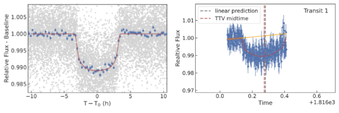
Compositional variations within the TRAPPIST-1 planetsFri, 13 Sep, 14:30–16:00 (CEST) | Poster area Level 2 – Galerie | P47
EXOA12 | Protoplanetary disks and planetesimal formation
EPSC2024-953 | Posters | EXOA12 | OPC: evaluations required
Comparative analysis of a binary system HD 135344 with a protoplanetary diskFri, 13 Sep, 10:30–12:00 (CEST) | Poster area Level 2 – Galerie | P52
EPSC2024-1112 | Posters | EXOA12 | OPC: evaluations required
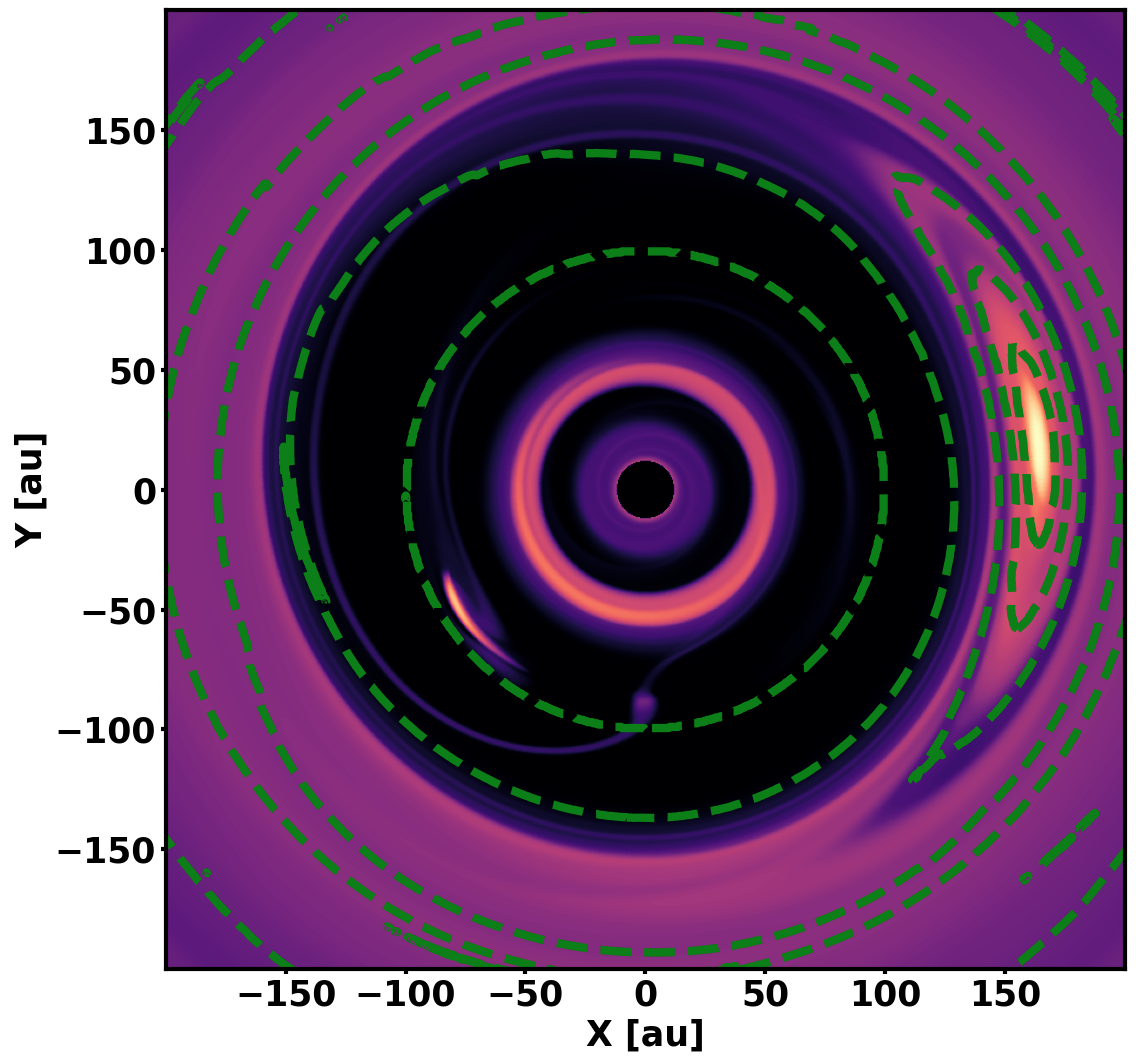
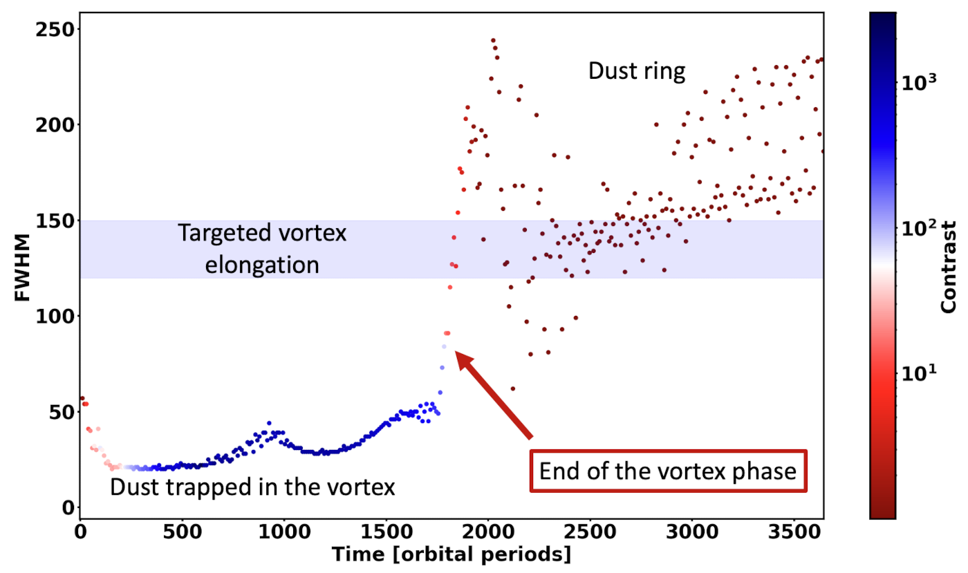
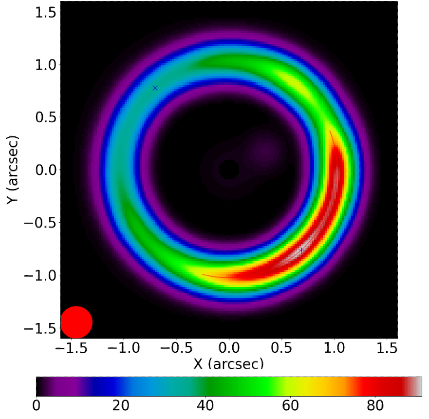
Planet-disk interactions in the AB Aurigae system: revisiting the hypothetical vortexFri, 13 Sep, 10:30–12:00 (CEST) | Poster area Level 2 – Galerie | P56
EPSC2024-1204 | ECP | Posters | EXOA12 | OPC: evaluations required
Radiation hydrodynamics of protoplanetary disks with frequency-dependent dust opacitiesFri, 13 Sep, 10:30–12:00 (CEST) | Poster area Level 2 – Galerie | P53