OPC applications
TP0 | General Session of TP
EPSC-DPS2025-1808 | Posters | TP0 | OPC: evaluations required
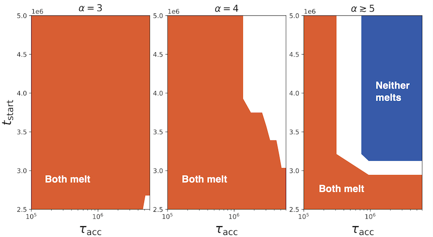
Consequences of imperfect accretion in the early giant planet instabilitymodelThu, 11 Sep, 18:00–19:30 (EEST) Finlandia Hall foyer | F4

TP1 | Mars Surface and Interior
EPSC-DPS2025-105 | ECP | Posters | TP1 | OPC: evaluations required
Dielectric Properties of Magnesium and Calcium Perchlorate Solutions: Implications for Subglacial Liquid Water on MarsThu, 11 Sep, 18:00–19:30 (EEST) Finlandia Hall foyer | F6


EPSC-DPS2025-398 | ECP | Posters | TP1
Preliminary analysis of aeolian bedforms present in the Eberswalde preserved delta, MarsThu, 11 Sep, 18:00–19:30 (EEST) Finlandia Hall foyer | F13
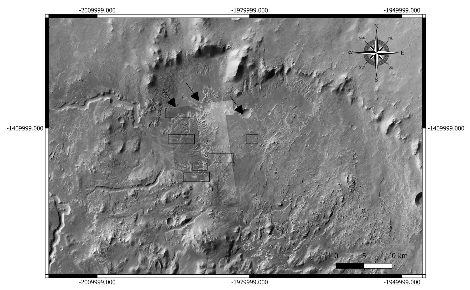
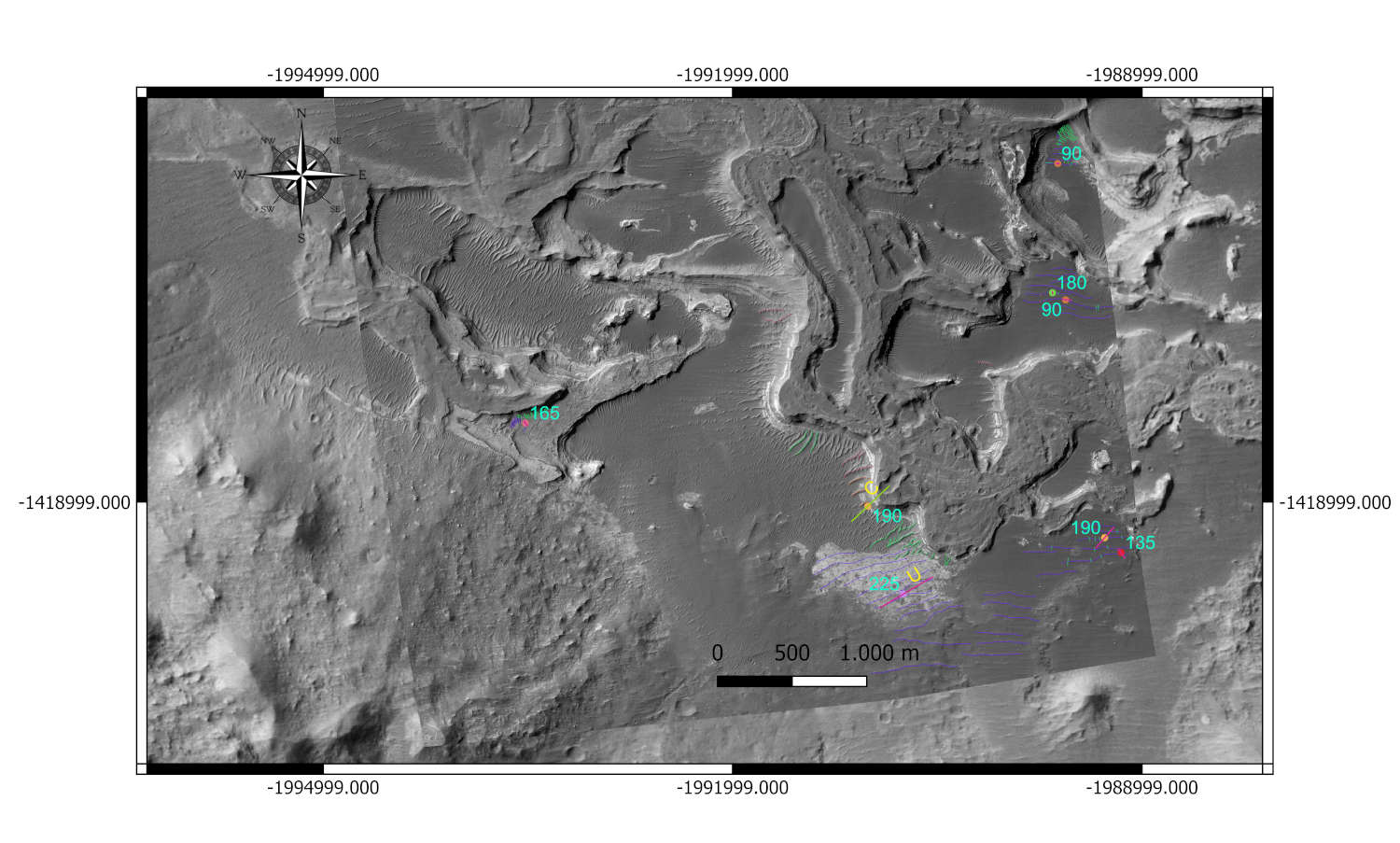
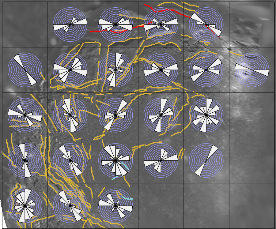
 Figure 2. Overview showing principal parameters across multiple areas, C= certain, U=uncertain,?= indefinite. Numerical values in degrees (°). (HiRISE DEM + CTX).
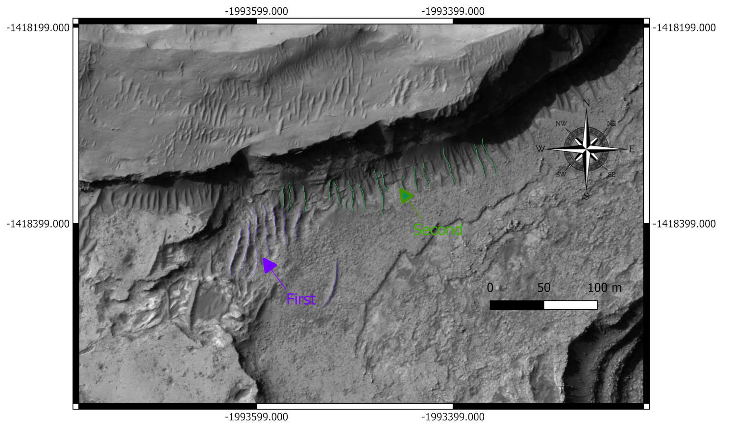
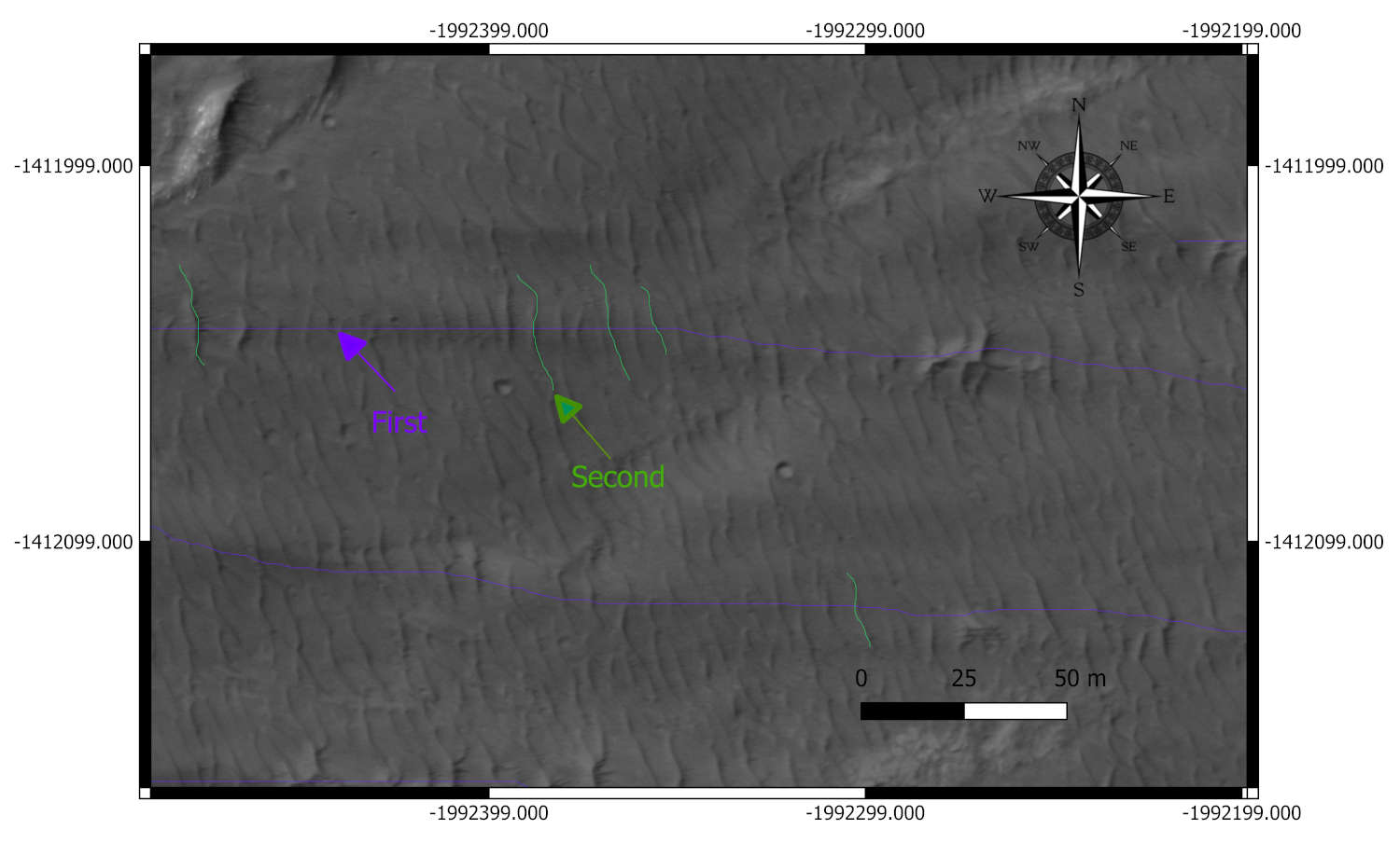
 Figure 3. The coexistence of first bedforms and second. HiRISE DEM.
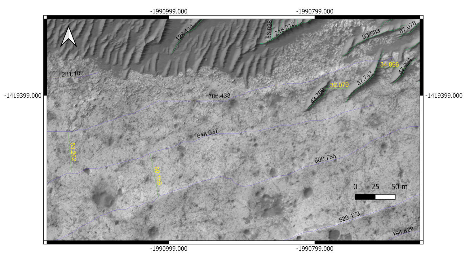
 Figure 4. Detailed view with measured crest lengths (black) and wavelengths (yellow). HiRISE DEM.
EPSC-DPS2025-1469 | Posters | TP1 | OPC: evaluations required
Controlled DTM and orthoimages mosaics from ExoMars TGO CaSSIS stereo-pairsThu, 11 Sep, 18:00–19:30 (EEST) Finlandia Hall foyer | F26
TP2 | Atmospheres and Exospheres of Terrestrial Bodies
EPSC-DPS2025-551 | ECP | Posters | TP2
Investigating the Reactivity of Excited State Sulfur Dioxide in the Atmosphere of VenusTue, 09 Sep, 18:00–19:30 (EEST) Finlandia Hall foyer | F2
EPSC-DPS2025-755 | ECP | Posters | TP2 | OPC: evaluations required
Exploring the variability of the meteoric metal layers in the Venusian atmosphereTue, 09 Sep, 18:00–19:30 (EEST) Finlandia Hall foyer | F12
EPSC-DPS2025-794 | ECP | Posters | TP2 | OPC: evaluations required
Investigating Martian Meteoric Metal Variability Through the Intercomparison of MAVEN/NGIMS Deep Dip Data and PCM-Mars Simulations.Tue, 09 Sep, 18:00–19:30 (EEST) Finlandia Hall foyer | F11
EPSC-DPS2025-1332 | ECP | Posters | TP2
Impact of water supply from interplanetary dust particles on the vertical D/H ratio profile of the Martian atmosphereTue, 09 Sep, 18:00–19:30 (EEST) Finlandia Hall foyer | F15
TP3 | Impact processes in the Solar System
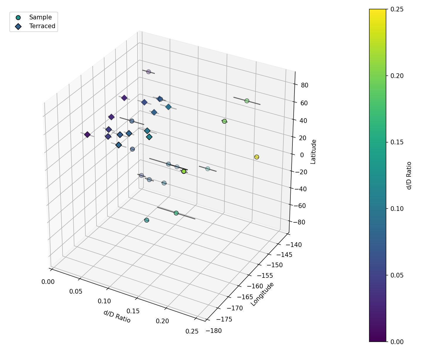
EPSC-DPS2025-729 | ECP | Posters | TP3 | OPC: evaluations required
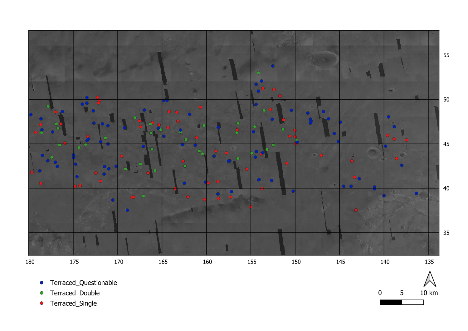
Analysis of terraced craters in Arcadia PlanitiaMon, 08 Sep, 18:00–19:30 (EEST) Finlandia Hall foyer | F8
EPSC-DPS2025-1580 | ECP | Posters | TP3
Experimental ice:silicate craters and their application to MarsMon, 08 Sep, 18:00–19:30 (EEST) Finlandia Hall foyer | F7


TP4 | Exploring Venus: Unveiling Mysteries of Earth’s Twin from Core to Atmosphere
EPSC-DPS2025-148 | Posters | TP4 | OPC: evaluations required
Investigating the Origin of Venus’ Clouds Using a Cloud Microphysics ModelMon, 08 Sep, 18:00–19:30 (EEST) Finlandia Hall foyer | F28

EPSC-DPS2025-679 | ECP | Posters | TP4
Reduced water loss due to atmospheric photochemistry under a runaway greenhouse condition on VenusMon, 08 Sep, 18:00–19:30 (EEST) Finlandia Hall foyer | F26
EPSC-DPS2025-718 | ECP | Posters | TP4 | OPC: evaluations required
Measurement of the spin of Venus using radio tracking data from Venus Express and expected outcomes from EnVisionMon, 08 Sep, 18:00–19:30 (EEST) Finlandia Hall foyer | F49

EPSC-DPS2025-1241 | ECP | Posters | TP4 | OPC: evaluations required
Thermal anomaly on Venus’s mesosphereMon, 08 Sep, 18:00–19:30 (EEST) Finlandia Hall foyer | F22
EPSC-DPS2025-1518 | ECP | Posters | TP4
Tesserae extension estimation and comparison with crustal plateau thickness, VenusMon, 08 Sep, 18:00–19:30 (EEST) Finlandia Hall foyer | F41
EPSC-DPS2025-1946 | ECP | Posters | TP4 | OPC: evaluations required
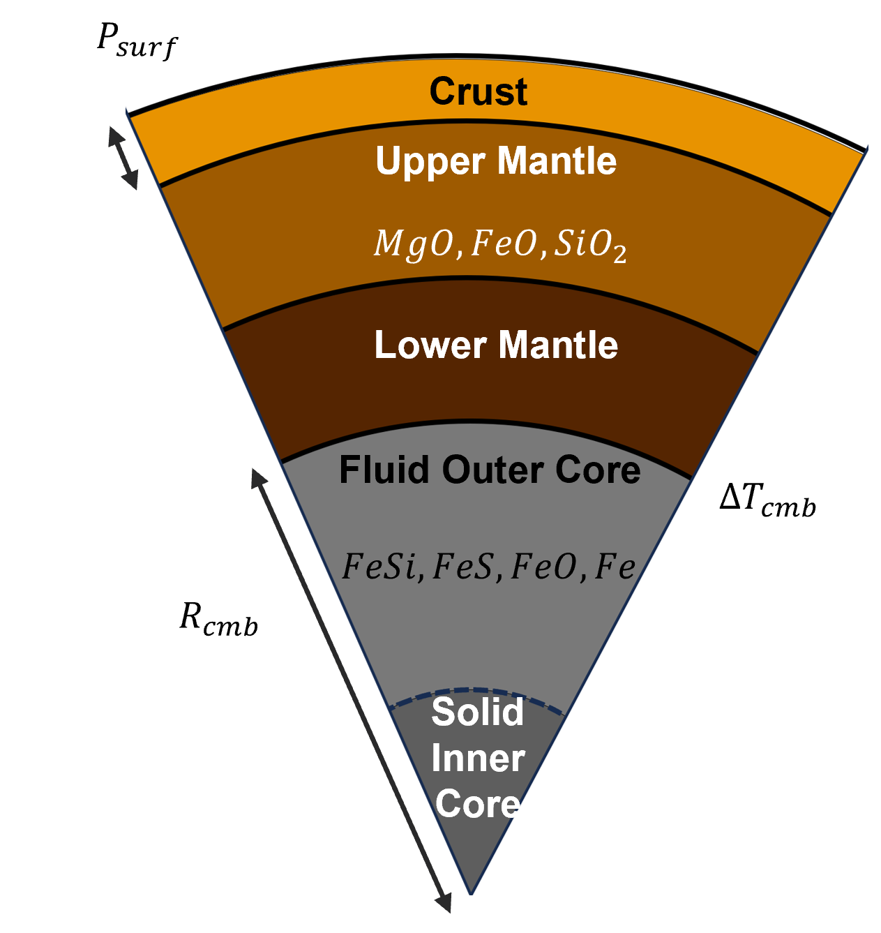
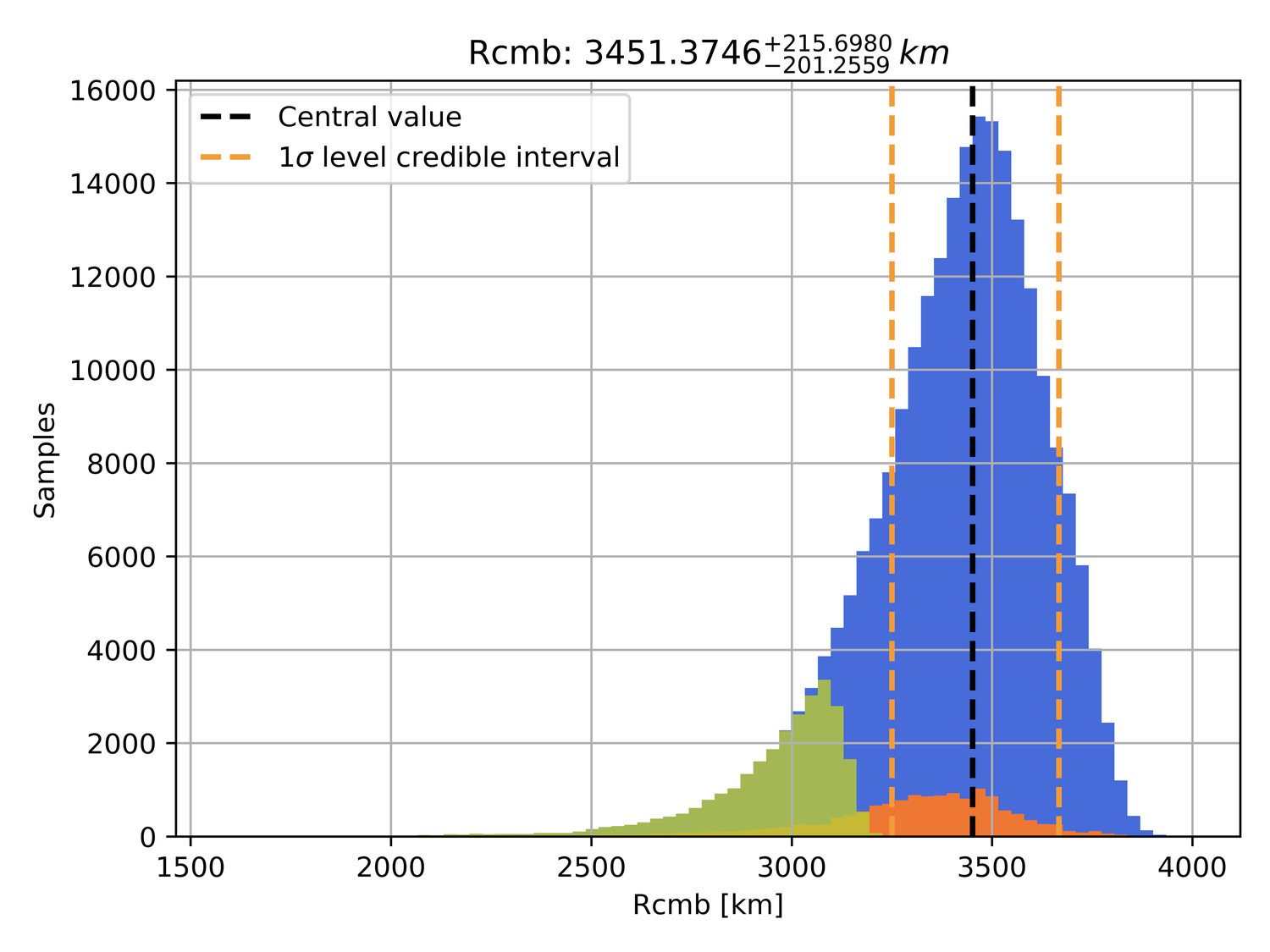
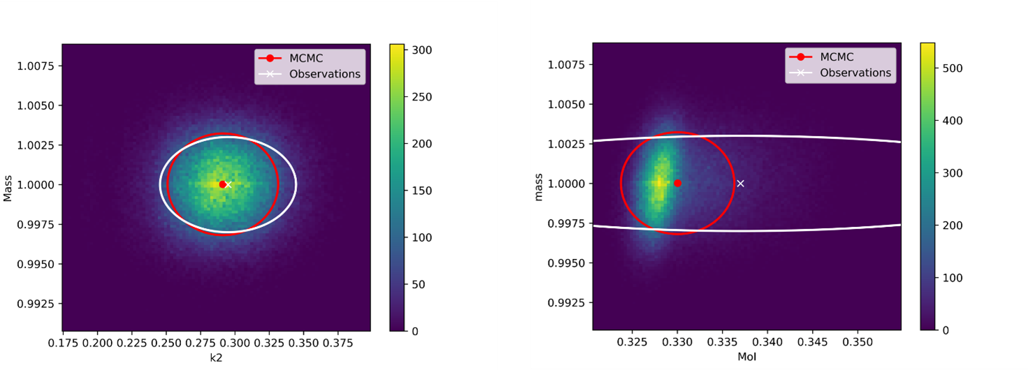
Inferring Venus interior structure based on present geophysical constraintsMon, 08 Sep, 18:00–19:30 (EEST) Finlandia Hall foyer | F48
TP5 | Planetary volcanism, tectonics, and seismicity
EPSC-DPS2025-474 | ECP | Posters | TP5
Hectometric-scale mounds on Mars: insights from Bernard Crater and surrounding terrains in Terra Sirenum, MarsTue, 09 Sep, 18:00–19:30 (EEST) Finlandia Hall foyer | F39
EPSC-DPS2025-1726 | ECP | Posters | TP5
Reconstructing Displacement Histories at Fault–Crater Intersections on Mercury.Tue, 09 Sep, 18:00–19:30 (EEST) Finlandia Hall foyer | F42
TP6 | Past, present and future landed missions on Mars and its satellites
EPSC-DPS2025-613 | ECP | Posters | TP6 | OPC: evaluations required
Gas mixing at Martian atmospheric conditions through a Smoothed Particle Hydrodynamics approachThu, 11 Sep, 18:00–19:30 (EEST) Finlandia Hall foyer | F31


EPSC-DPS2025-1752 | ECP | Posters | TP6 | OPC: evaluations required
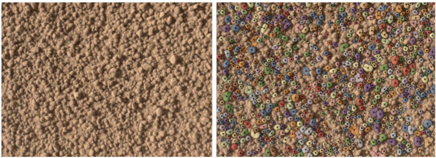
From Imagery to Insight: Machine Learning for Grain-Scale Sediment Analysis on MarsThu, 11 Sep, 18:00–19:30 (EEST) Finlandia Hall foyer | F38
EPSC-DPS2025-1775 | ECP | Posters | TP6 | OPC: evaluations required
Preliminary Feasibility Assessment of the Tumbleweed Rover Platform and Mission using the AU Planetary Environment FacilityThu, 11 Sep, 18:00–19:30 (EEST) Finlandia Hall foyer | F45
TP7 | Ionospheres of unmagnetized or weakly magnetized bodies
EPSC-DPS2025-214 | ECP | Posters | TP7
Statistical Study on the Solar Wind Turbulence Spectra upstream of MarsMon, 08 Sep, 18:00–19:30 (EEST) Finlandia Hall foyer | F62
EPSC-DPS2025-572 | ECP | Posters | TP7 | OPC: evaluations required
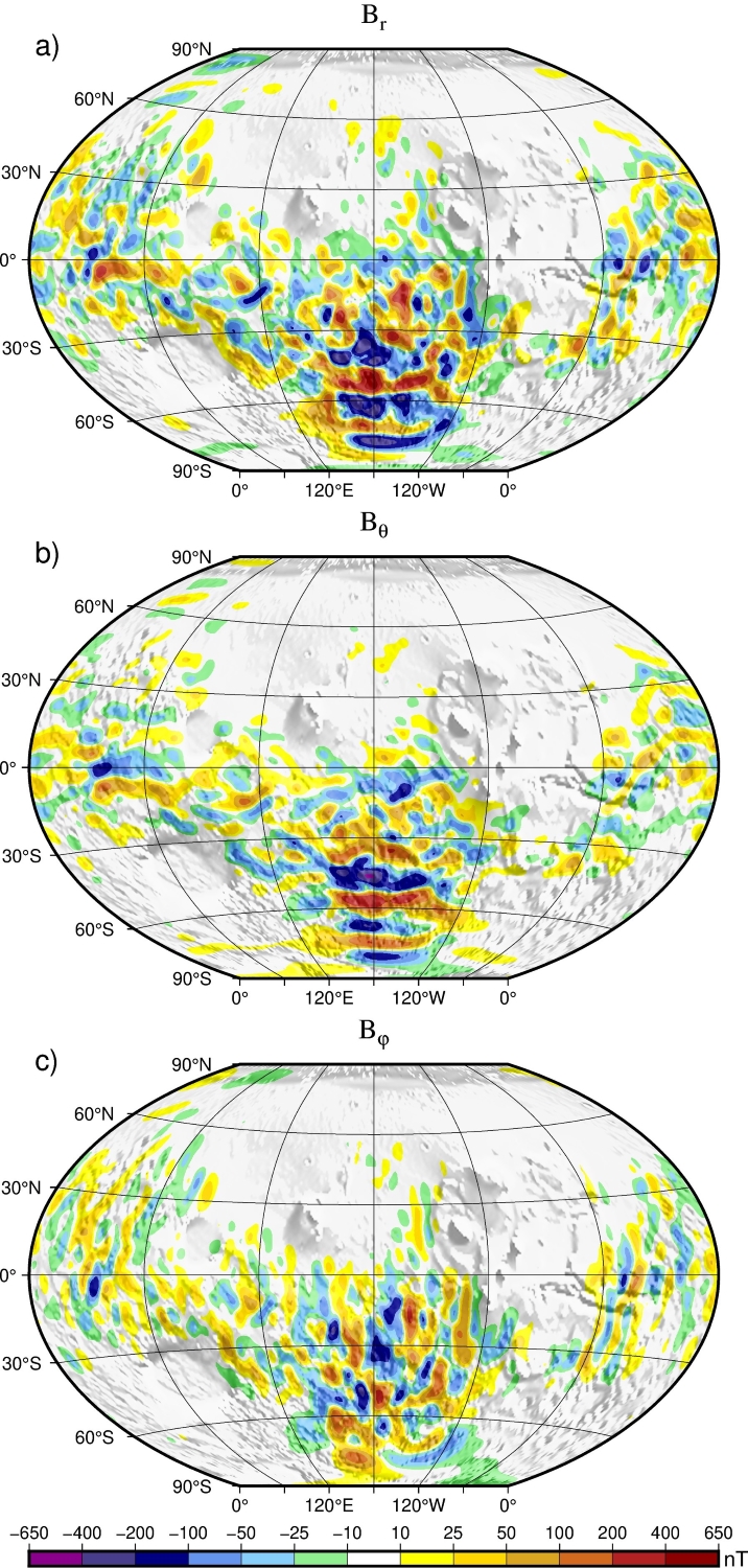
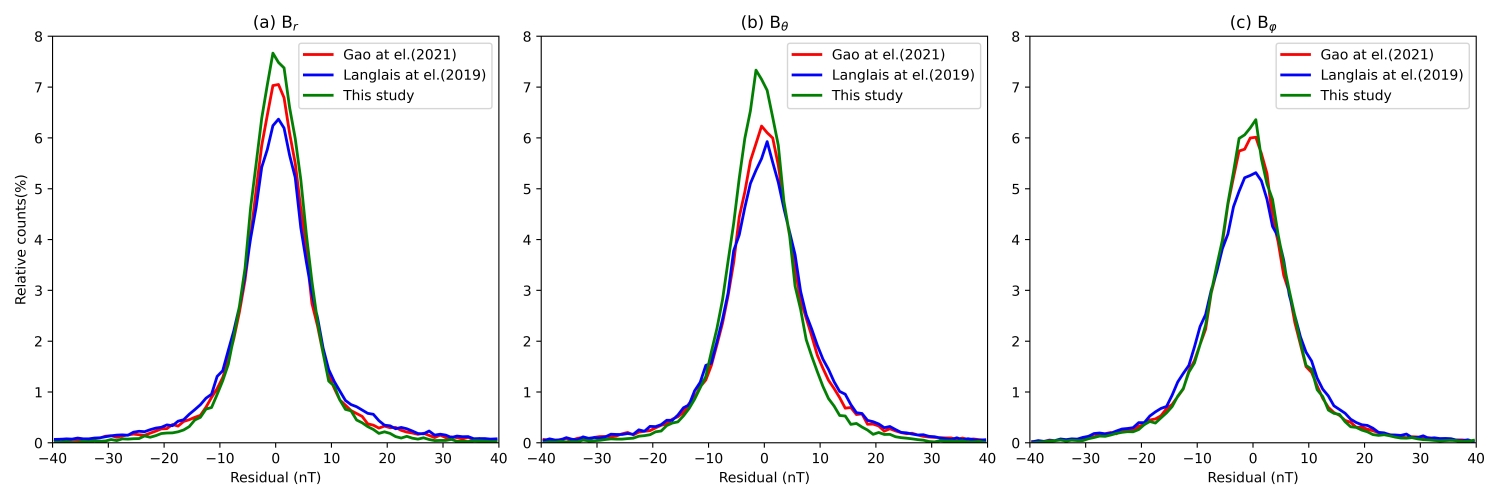
Modeling the Martian Crustal Magnetic Field Using Data from MGS, MAVEN, and Tianwen-1Mon, 08 Sep, 18:00–19:30 (EEST) Finlandia Hall foyer | F55
EPSC-DPS2025-832 | ECP | Posters | TP7 | OPC: evaluations required
Photoionization and photodissociation rates across a solar cycleMon, 08 Sep, 18:00–19:30 (EEST) Finlandia Hall foyer | F66
TP8 | The Multi-Scale Physics of Surface-Bounded Exosphere and Surface Interactions
EPSC-DPS2025-748 | Posters | TP8 | OPC: evaluations required
Atomic Scale Modelling of Icy Surfaces: A Best Practice for Validating Interatomic Potentials and Ice Substrates in Extreme EnvironmentsMon, 08 Sep, 18:00–19:30 (EEST) Finlandia Hall foyer | F74
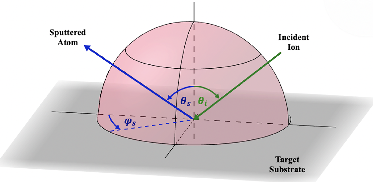
EPSC-DPS2025-1193 | ECP | Posters | TP8 | OPC: evaluations required
Solar Wind-Induced Sputtering: Investigating Anisotropy in the Angular Distribution of Ejecta using SDTrimSPMon, 08 Sep, 18:00–19:30 (EEST) Finlandia Hall foyer | F75
EPSC-DPS2025-1690 | ECP | Posters | TP8
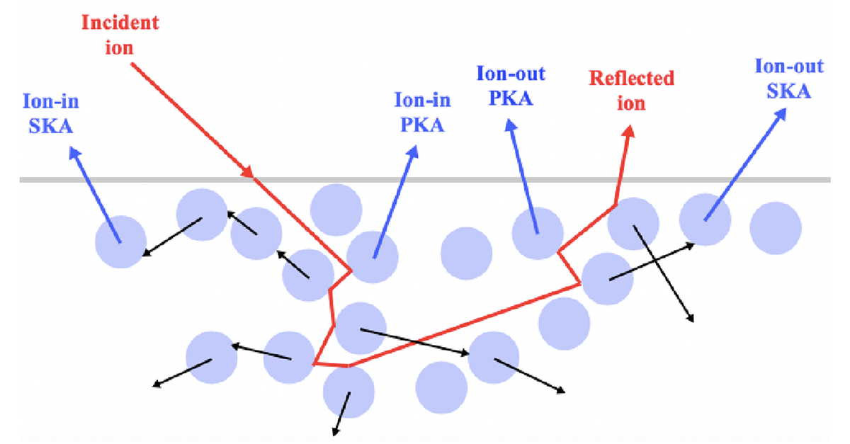
Understanding the energy spectra of scattered solar wind ions using low energy ion scatteringMon, 08 Sep, 18:00–19:30 (EEST) Finlandia Hall foyer | F71
TP9 | On the Quest to Solve Mercury's Secrets
EPSC-DPS2025-256 | ECP | Posters | TP9
Deep learning map of fresh crater ejecta on Mercury: a resource for space weathering studiesThu, 11 Sep, 18:00–19:30 (EEST) Finlandia Hall foyer | F60
EPSC-DPS2025-687 | ECP | Posters | TP9
Status Update on Strofio: Recovery and Performance Advancements Post-Launch AnomalyThu, 11 Sep, 18:00–19:30 (EEST) Finlandia Hall foyer | F62
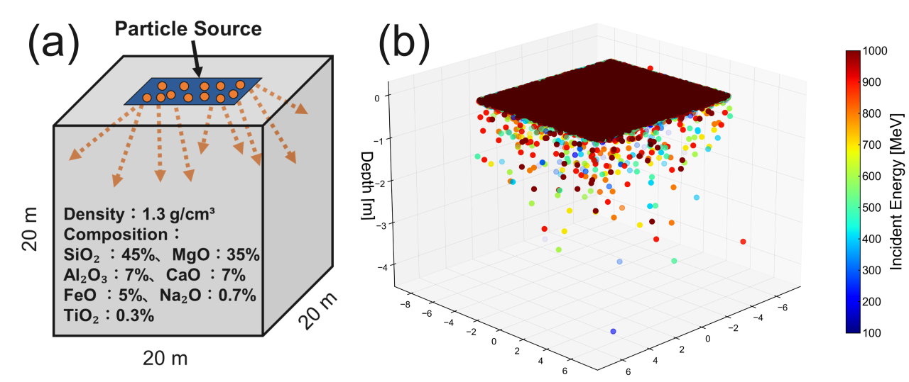
EPSC-DPS2025-712 | ECP | Posters | TP9
Assessment of Cosmic-Ray-Induced Space Weathering on Mercury’s Surface Using Geant4 SimulationsThu, 11 Sep, 18:00–19:30 (EEST) Finlandia Hall foyer | F61
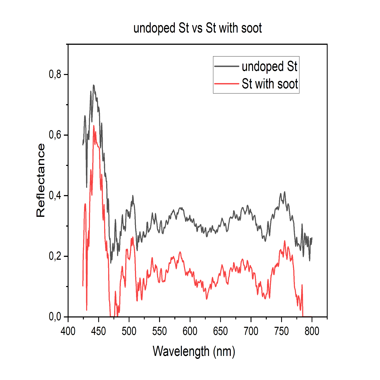
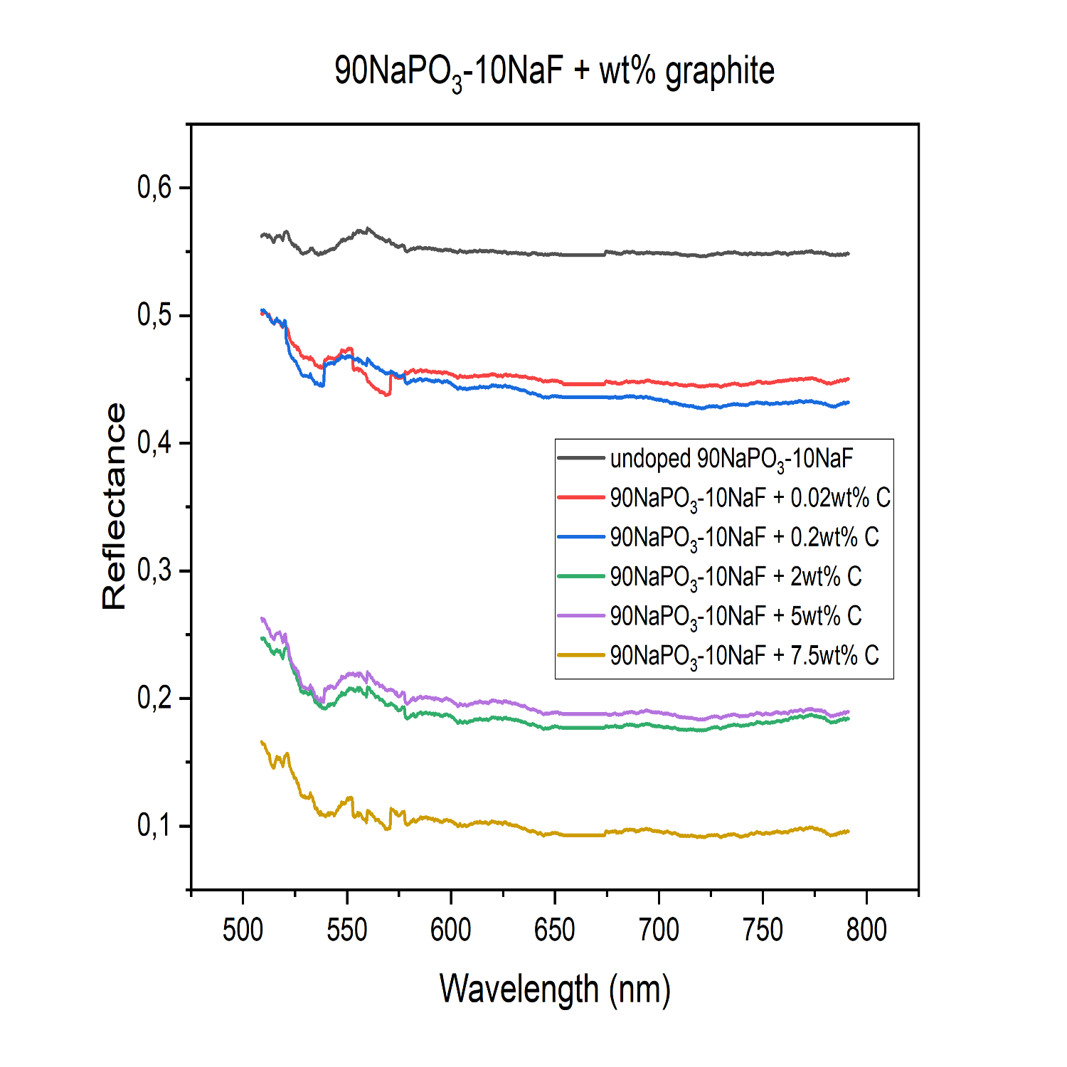
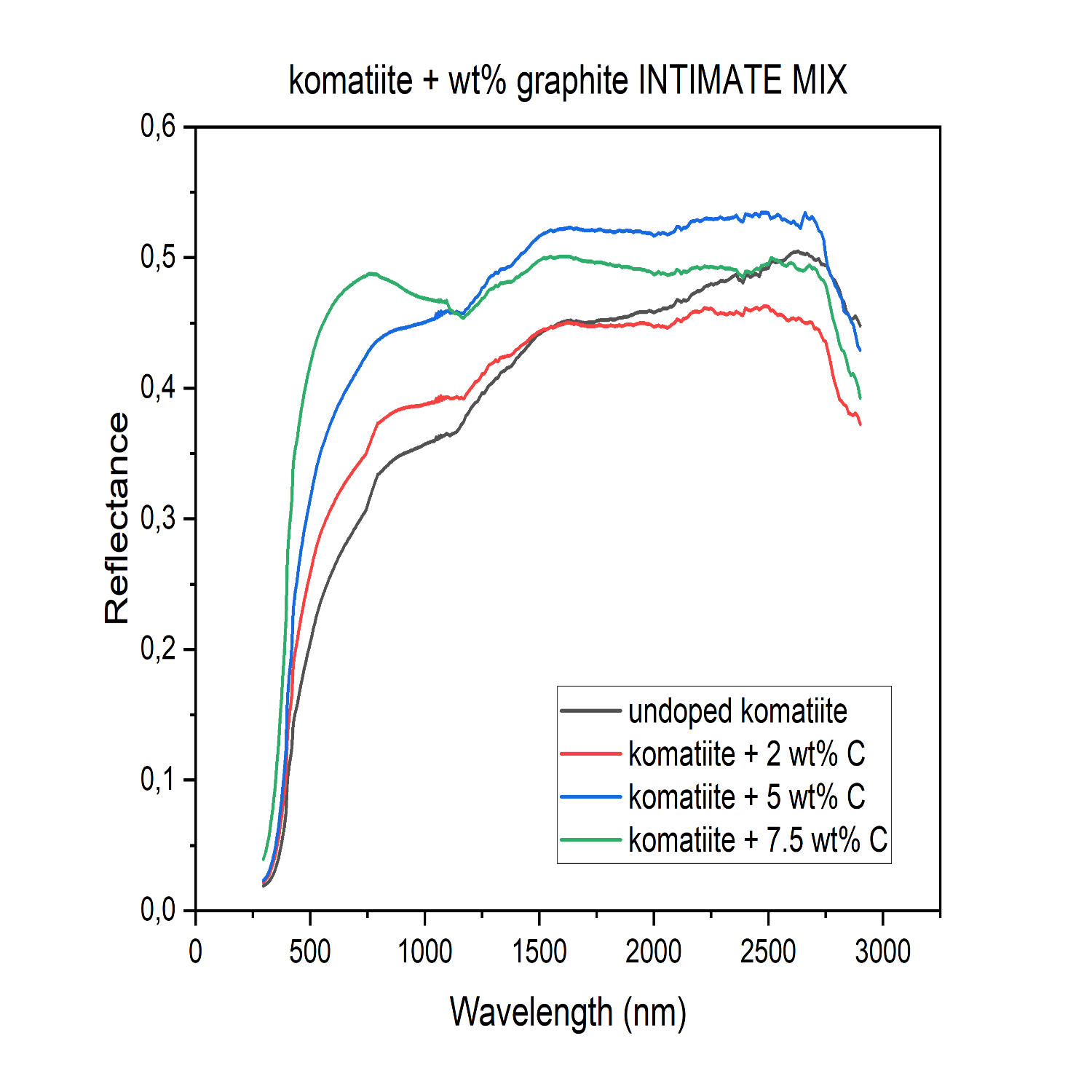
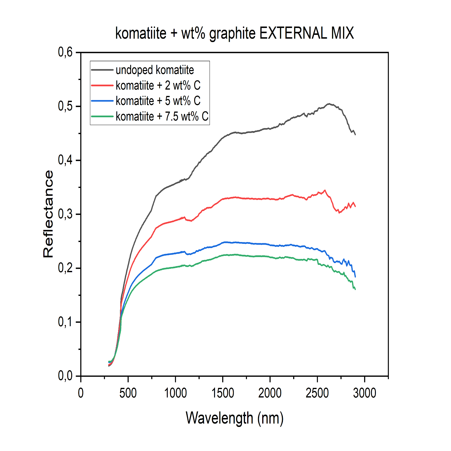
EPSC-DPS2025-1361 | Posters | TP9
Mercury surface UV-Vis-NIR spectral reflectance: Role of GraphiteThu, 11 Sep, 18:00–19:30 (EEST) Finlandia Hall foyer | F51
EPSC-DPS2025-1516 | ECP | Posters | TP9
Spectral fingerprints of pure and mixed minerals: Laboratory characterization and ML IntegrationThu, 11 Sep, 18:00–19:30 (EEST) Finlandia Hall foyer | F50
TP10 | Planetary Cryospheres: Ices in the Solar System
EPSC-DPS2025-301 | ECP | Posters | TP10
Low-temperature hyper-spectral acquisitions of slabs with water ice and Martian simulant MGS-1.Tue, 09 Sep, 18:00–19:30 (EEST) Finlandia Hall foyer | F45
TP11 | Lunar Space Environment
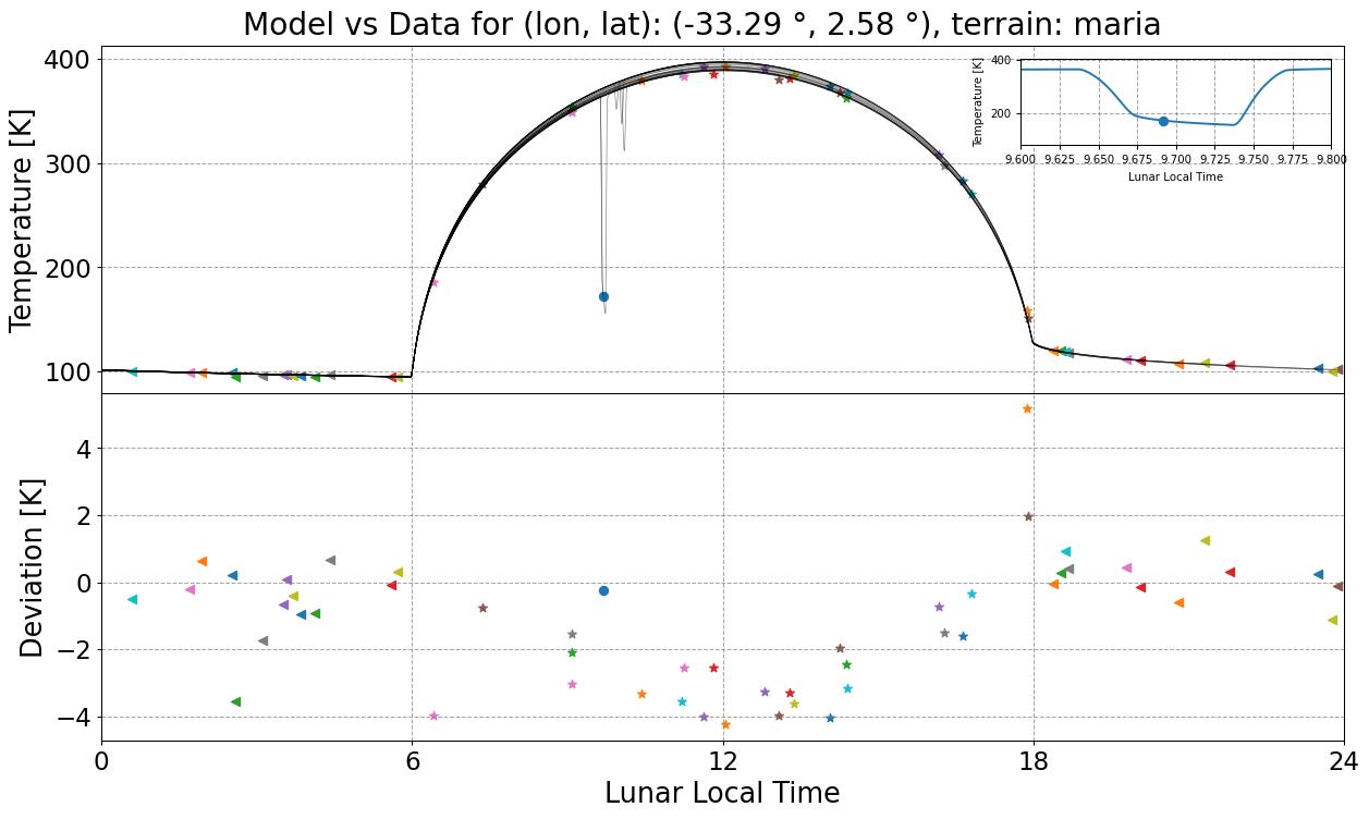
EPSC-DPS2025-1060 | ECP | Posters | TP11 | OPC: evaluations required
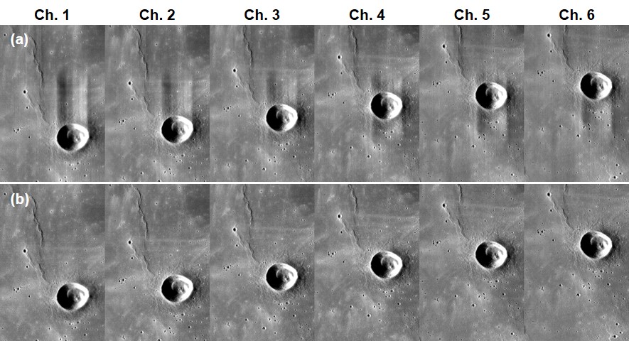
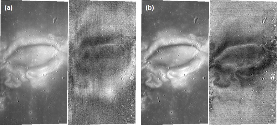
Refining a Thermophysical Model of the Lunar Surface using EclipsesThu, 11 Sep, 18:00–19:30 (EEST) Finlandia Hall foyer | F79
TP13 | Planetary Dynamics: Shape, Gravity, Orbit, Tides, and Rotation from Observations and Models
EPSC-DPS2025-1502 | ECP | Posters | TP13
High-resolution Shape Modeling of Ryugu from an Improved Neural Implicit MethodTue, 09 Sep, 18:00–19:30 (EEST) Finlandia Hall foyer | F64
OPS1 | Unveiling the Jovian Moons: Juno’s view of Io, Europa, and Ganymede
EPSC-DPS2025-996 | ECP | Posters | OPS1 | OPC: evaluations required
Evaluating Multi-Spacecraft Stereo Imaging for DEM Generation on GanymedeTue, 09 Sep, 18:00–19:30 (EEST) Lämpiö foyer | L2
EPSC-DPS2025-999 | ECP | Posters | OPS1 | OPC: evaluations required
Europa's Variable Alkali Exosphere After the Juno 2022 FlybyTue, 09 Sep, 18:00–19:30 (EEST) Lämpiö foyer | L3
OPS2 | Icy Moons and Ocean Worlds in the Era of Juice and Europa Clipper
EPSC-DPS2025-90 | ECP | Posters | OPS2 | OPC: evaluations required
Ray Tracing for Titan’s Ionospheric Occultation of Saturn Radio Emissions: Implications for JUICE MissionMon, 08 Sep, 18:00–19:30 (EEST) Lämpiö foyer | L28
EPSC-DPS2025-94 | ECP | Posters | OPS2
Role of carbon in the interior structure of Jupiter’s moons Europa and IoMon, 08 Sep, 18:00–19:30 (EEST) Lämpiö foyer | L1
EPSC-DPS2025-601 | ECP | Posters | OPS2 | OPC: evaluations required
Thermal Surface Measurements of Europa using Galileo PPR: Searching for Temperature AnomaliesMon, 08 Sep, 18:00–19:30 (EEST) Lämpiö foyer | L11
EPSC-DPS2025-646 | ECP | Posters | OPS2 | OPC: evaluations required
Carbon-rich interiors of Ganymede and Titan: application of a kinetic model of carbonaceous organic matter transformationMon, 08 Sep, 18:00–19:30 (EEST) Lämpiö foyer | L10
EPSC-DPS2025-656 | ECP | Posters | OPS2 | OPC: evaluations required
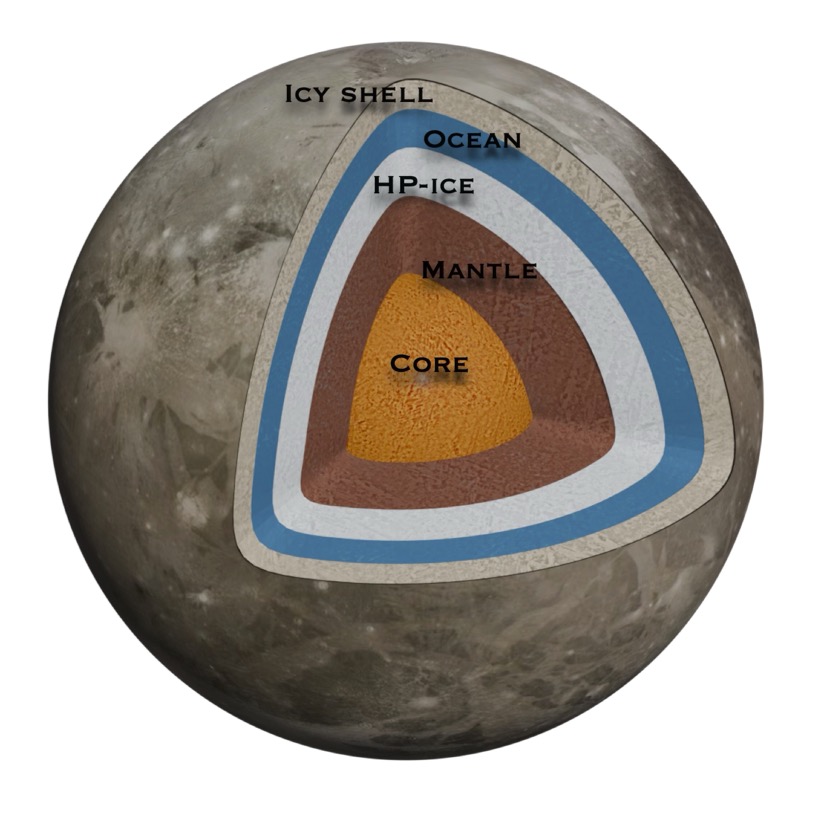
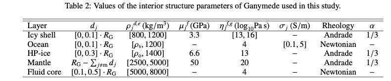
Interior structure models and tidal Love numbers of Ganymede, Callisto and Titan: A prospective study for JUICE and DragonflyMon, 08 Sep, 18:00–19:30 (EEST) Lämpiö foyer | L14
EPSC-DPS2025-777 | ECP | Posters | OPS2
Formation Conditions Leading to an Unmelted Callisto and a Differentiated GanymedeMon, 08 Sep, 18:00–19:30 (EEST) Lämpiö foyer | L15
EPSC-DPS2025-899 | ECP | Posters | OPS2
DSMC Modelling of Gaseous Plumes in Europa’s Icy VentsMon, 08 Sep, 18:00–19:30 (EEST) Lämpiö foyer | L17
EPSC-DPS2025-1360 | ECP | Posters | OPS2 | OPC: evaluations required
New Mathematical Tool For Icy Moon Exploration: Spherical Iterative Filtering For Gravimetric Data And The Study Case Of GanymedeMon, 08 Sep, 18:00–19:30 (EEST) Lämpiö foyer | L18
EPSC-DPS2025-1570 | ECP | Posters | OPS2 | OPC: evaluations required
Modeling the interactions between Callisto’s neutral and ionized environments and the Jovian magnetosphereMon, 08 Sep, 18:00–19:30 (EEST) Lämpiö foyer | L31
OPS3 | Jupiter’s Magnetosphere in the Juno Era and beyond: Insights from In-Situ and remote sensing Exploration
EPSC-DPS2025-525 | ECP | Posters | OPS3 | OPC: evaluations required
Stochastic Modelling of Jupiter's MagnetosphereThu, 11 Sep, 18:00–19:30 (EEST) Lämpiö foyer | L4
EPSC-DPS2025-713 | ECP | Posters | OPS3 | OPC: evaluations required
Radio occultation experiments of the Io plasma torus: from Juno to JUICEThu, 11 Sep, 18:00–19:30 (EEST) Lämpiö foyer | L5
EPSC-DPS2025-1140 | ECP | Posters | OPS3 | OPC: evaluations required
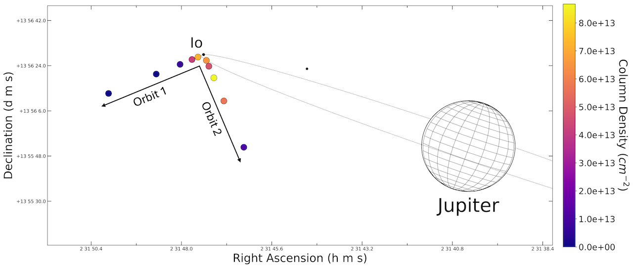
Constraining the Spatial Profile of Oxygen in Io’s Neutral Cloud with HST’s Cosmic Origins Spectrograph.Thu, 11 Sep, 18:00–19:30 (EEST) Lämpiö foyer | L10
EPSC-DPS2025-1463 | Posters | OPS3 | OPC: evaluations required
Analysis of Io’s far-ultraviolet emission morphology using HST STIS spectral imaging data from 1997 to presentThu, 11 Sep, 18:00–19:30 (EEST) Lämpiö foyer | L11
EPSC-DPS2025-1569 | ECP | Posters | OPS3 | OPC: evaluations required
Electron distribution in the Jovian inner magnetosphere derived from multiple observationsThu, 11 Sep, 18:00–19:30 (EEST) Lämpiö foyer | L12
OPS4 | Exploring the Saturn system
EPSC-DPS2025-544 | Posters | OPS4 | OPC: evaluations required
Towards understanding mass spectra from icy moons using quantum chemistry: A case study for aromatic compounds.Tue, 09 Sep, 18:00–19:30 (EEST) Lämpiö foyer | L16
EPSC-DPS2025-1574 | Posters | OPS4
Ozone in Planetary Ices: Solid-State Detection under Enceladus-like conditionsTue, 09 Sep, 18:00–19:30 (EEST) Lämpiö foyer | L17
EPSC-DPS2025-1769 | ECP | Posters | OPS4 | OPC: evaluations required
Evolution of Viscous Overstability in Saturn’s Rings:Insights from Large-Scale N-Body SimulationsTue, 09 Sep, 18:00–19:30 (EEST) Lämpiö foyer | L27
EPSC-DPS2025-1889 | ECP | Posters | OPS4 | OPC: evaluations required
Constraining Enceladus' interior structure by using libration measurement in a Bayesian frameworkTue, 09 Sep, 18:00–19:30 (EEST) Lämpiö foyer | L20
OPS5 | Exploration of Titan
EPSC-DPS2025-85 | ECP | Posters | OPS5 | OPC: evaluations required
Modeling Atmospheric Alteration on Titan: Hydrodynamics and Shock-Induced Chemistry of Meteoroid EntryMon, 08 Sep, 18:00–19:30 (EEST) Lämpiö foyer | L46

EPSC-DPS2025-108 | ECP | Posters | OPS5
Cloud formation and composition on Titan with a Planetary Climate ModelMon, 08 Sep, 18:00–19:30 (EEST) Lämpiö foyer | L39

OPS6 | Ice Giant Systems: Science and Exploration
EPSC-DPS2025-693 | Posters | OPS6 | OPC: evaluations required
First Observations of Uranus’ H3+ Vertical Profiles with JWSTThu, 11 Sep, 18:00–19:30 (EEST) Lämpiö foyer | L26
EPSC-DPS2025-1554 | ECP | Posters | OPS6 | OPC: evaluations required
Surface investigation of Ariel’s structural featuresThu, 11 Sep, 18:00–19:30 (EEST) Lämpiö foyer | L24
OPS7 | Aerosols and clouds in planetary atmospheres
EPSC-DPS2025-204 | ECP | Posters | OPS7 | OPC: evaluations required
Bridging Chemistry and Technology: The Dual Role of PAHs in Exoplanetary AtmospheresTue, 09 Sep, 18:00–19:30 (EEST) Lämpiö foyer | L38
EPSC-DPS2025-420 | ECP | Posters | OPS7 | OPC: evaluations required
Revealing patchy clouds on WASP-43b and WASP-121b through coupled microphysical and hydrodynamical modelsTue, 09 Sep, 18:00–19:30 (EEST) Lämpiö foyer | L41
EPSC-DPS2025-453 | ECP | Posters | OPS7
Reactive uptake of SO2 in H2SO4 droplets under Venus-analogous conditions: Laboratory study using a single particle levitation methodTue, 09 Sep, 18:00–19:30 (EEST) Lämpiö foyer | L29
EPSC-DPS2025-1094 | ECP | Posters | OPS7 | OPC: evaluations required
Clearing the Air: Solar System Bodies as Windows into the Impact of Aerosols on Exoplanet Atmospheric RetrievalsTue, 09 Sep, 18:00–19:30 (EEST) Lämpiö foyer | L39
OPS8 | Jupiter's and Saturn's Atmospheres
EPSC-DPS2025-143 | Posters | OPS8 | OPC: evaluations required
Jovian Zonal Winds Revealed from Cassini/VIMS ObservationsThu, 11 Sep, 18:00–19:30 (EEST) Lämpiö foyer | L36
EPSC-DPS2025-643 | ECP | Posters | OPS8 | OPC: evaluations required
Experimental study of the interference dips observed on the collision-induced absorption fundamental band of H2: their relevance to planetary atmosphere characterizationThu, 11 Sep, 18:00–19:30 (EEST) Lämpiö foyer | L46
EPSC-DPS2025-1624 | ECP | Posters | OPS8 | OPC: evaluations required
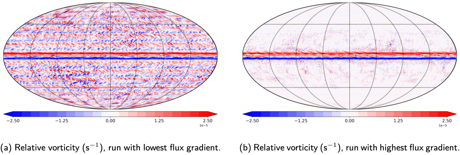
The Role of Bottom Thermal Forcing on Modulating Baroclinic Instability in a Jupiter GCMThu, 11 Sep, 18:00–19:30 (EEST) Lämpiö foyer | L45
OPS9 | Giant Planet Interiors, Atmospheres, and Evolution
EPSC-DPS2025-155 | ECP | Posters | OPS9 | OPC: evaluations required
Giant Planet Formation in the Solar SystemThu, 11 Sep, 18:00–19:30 (EEST) Lämpiö foyer | L51
EPSC-DPS2025-413 | ECP | Posters | OPS9
Toward a Comprehensive Global Climate Model of Uranus: Radiative-Convective and Dynamical SimulationsThu, 11 Sep, 18:00–19:30 (EEST) Lämpiö foyer | L50
EPSC-DPS2025-730 | ECP | Posters | OPS9 | OPC: evaluations required
Conditions for stable layers in Jupiter and Saturn over timeThu, 11 Sep, 18:00–19:30 (EEST) Lämpiö foyer | L53
EPSC-DPS2025-1293 | ECP | Posters | OPS9 | OPC: evaluations required
From Jupiter to Saturn: Characterizing Interior Structures with Machine LearningThu, 11 Sep, 18:00–19:30 (EEST) Lämpiö foyer | L49
MITM2 | Planetary Missions, Instrumentations, and mission concepts: new opportunities for planetary exploration
EPSC-DPS2025-65 | ECP | Posters | MITM2 | OPC: evaluations required
Modelling the Radiative Environment of the Lunar South Pole Aitken basin.Tue, 09 Sep, 18:00–19:30 (EEST) Finlandia Hall foyer | F66
EPSC-DPS2025-71 | ECP | Posters | MITM2 | OPC: evaluations required
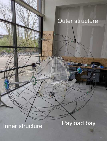
Flux Gate Magentometer and Boom for Cubesat Mission Beyond Low Earth OrbitTue, 09 Sep, 18:00–19:30 (EEST) Finlandia Hall foyer | F65
EPSC-DPS2025-156 | ECP | Posters | MITM2
Neptune Orbital Survey and TRiton Orbiter MissiOn (NOSTROMO): A Mission Concept to Explore the Neptune-Triton System.Tue, 09 Sep, 18:00–19:30 (EEST) Finlandia Hall foyer | F74

EPSC-DPS2025-298 | ECP | Posters | MITM2 | OPC: evaluations required
Long-Term Planning Framework and Key Scientific Inputs for the M-MATISSE missionTue, 09 Sep, 18:00–19:30 (EEST) Finlandia Hall foyer | F71
EPSC-DPS2025-874 | ECP | Posters | MITM2
SEAFARER: Navigating Unknown Seas An L4-class space mission concept for the exploration of the Saturnian System developed during the ESA 2024 Summer School AlpbachTue, 09 Sep, 18:00–19:30 (EEST) Finlandia Hall foyer | F82
MITM5 | Artificial Intelligence and Machine Learning in Planetary Science
EPSC-DPS2025-149 | ECP | Posters | MITM5 | OPC: evaluations required
Exploring the potential of neural networks in early detection of potentially hazardous Near-Earth ObjectsThu, 11 Sep, 18:00–19:30 (EEST) Finlandia Hall foyer | F83

EPSC-DPS2025-272 | ECP | Posters | MITM5 | OPC: evaluations required
Implementing a Neural Network on Forward Models:A Case study for Exoplanet AtmospheresThu, 11 Sep, 18:00–19:30 (EEST) Finlandia Hall foyer | F92
EPSC-DPS2025-691 | Posters | MITM5 | OPC: evaluations required
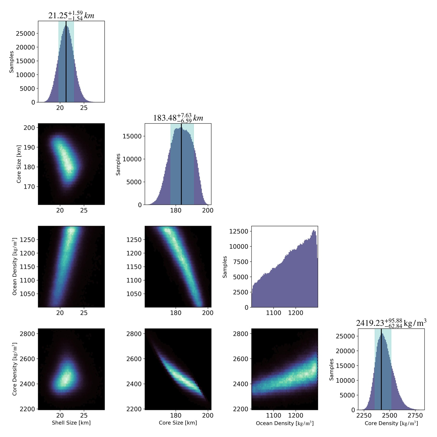
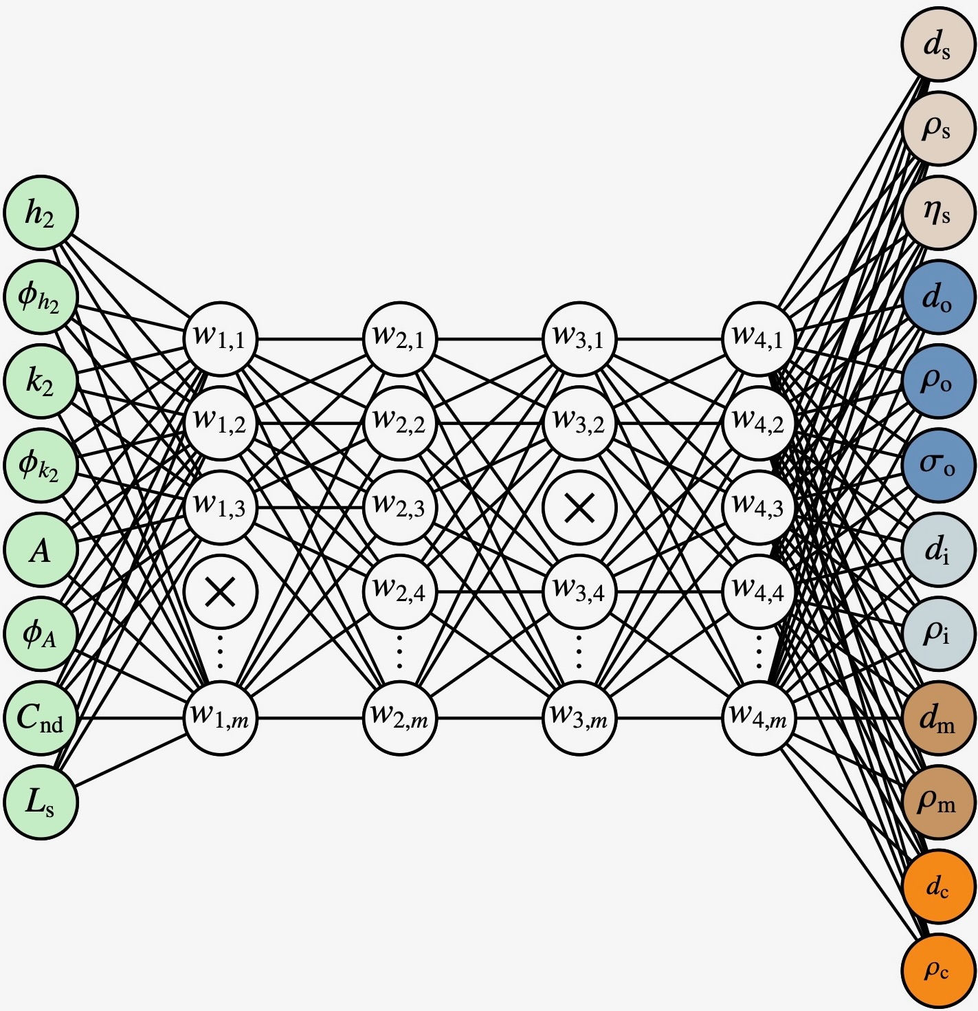
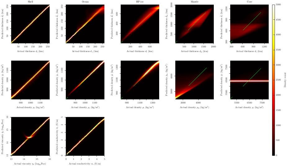
Enforcing multiple constraints on the interior structure of Ganymede: a machine learning approachThu, 11 Sep, 18:00–19:30 (EEST) Finlandia Hall foyer | F91

EPSC-DPS2025-709 | ECP | Posters | MITM5 | OPC: evaluations required
ThermoONet -- Deep Learning-based Small Body Thermophysical NetworkThu, 11 Sep, 18:00–19:30 (EEST) Finlandia Hall foyer | F84
EPSC-DPS2025-1703 | ECP | Posters | MITM5
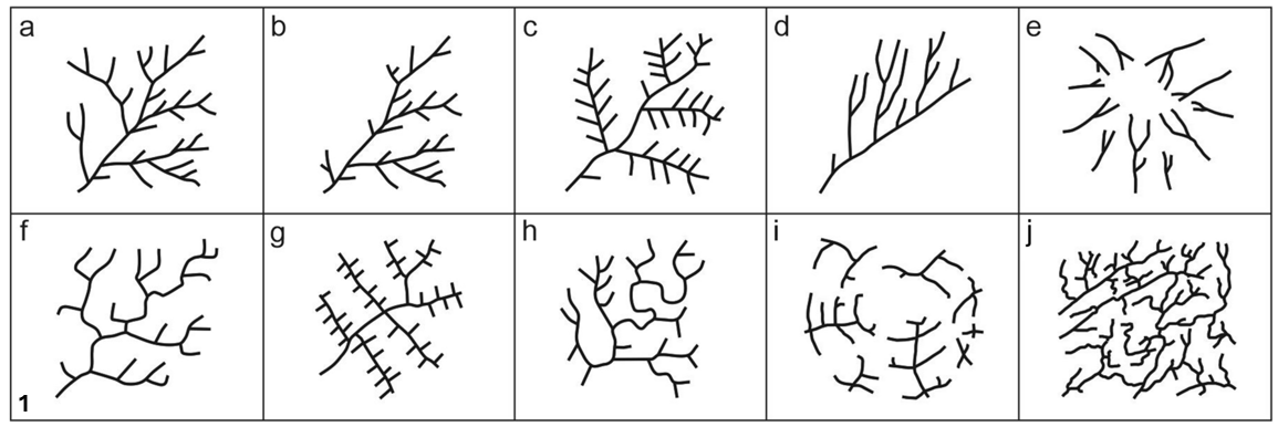
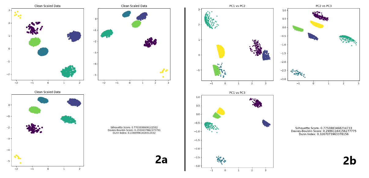
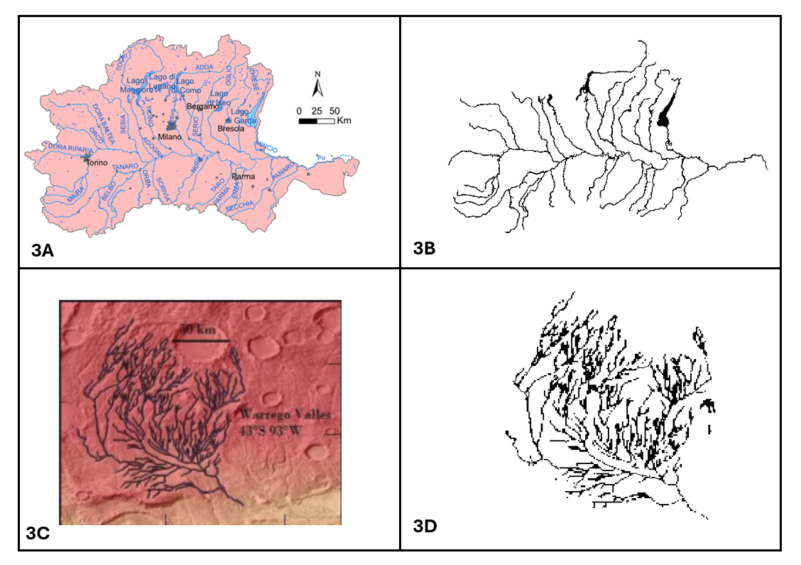
A Novel Machine Learning Approach for Objective Fluvial Network Classification: Earth & BeyondThu, 11 Sep, 18:00–19:30 (EEST) Finlandia Hall foyer | F87
MITM8 | Imagery, photometry, and spectroscopy of small bodies and planetary surfaces
EPSC-DPS2025-812 | ECP | Posters | MITM8 | OPC: evaluations required
A Spectral Comparison of Small Main Belt and Near-Earth V-types in the Near-InfraredTue, 09 Sep, 18:00–19:30 (EEST) Finlandia Hall foyer | F101
EPSC-DPS2025-945 | ECP | Posters | MITM8 | OPC: evaluations required
Hyperspectral Mineral Mapping for Sustainable Lunar Exploration: Targeting ISRU Resources in Key Lunar RegionsTue, 09 Sep, 18:00–19:30 (EEST) Finlandia Hall foyer | F102
EPSC-DPS2025-997 | ECP | Posters | MITM8 | OPC: evaluations required
A Pilot Rapid-Response Project to Characterize Small Near Earth Objectswith LCO’s MuSCAT Instruments.Tue, 09 Sep, 18:00–19:30 (EEST) Finlandia Hall foyer | F103
EPSC-DPS2025-1190 | ECP | Posters | MITM8 | OPC: evaluations required
Fluorescence Modelling and Spectroscopic Analysis of the NH2 Radical inCometary EnvironmentsTue, 09 Sep, 18:00–19:30 (EEST) Finlandia Hall foyer | F105
EPSC-DPS2025-1272 | ECP | Posters | MITM8 | OPC: evaluations required
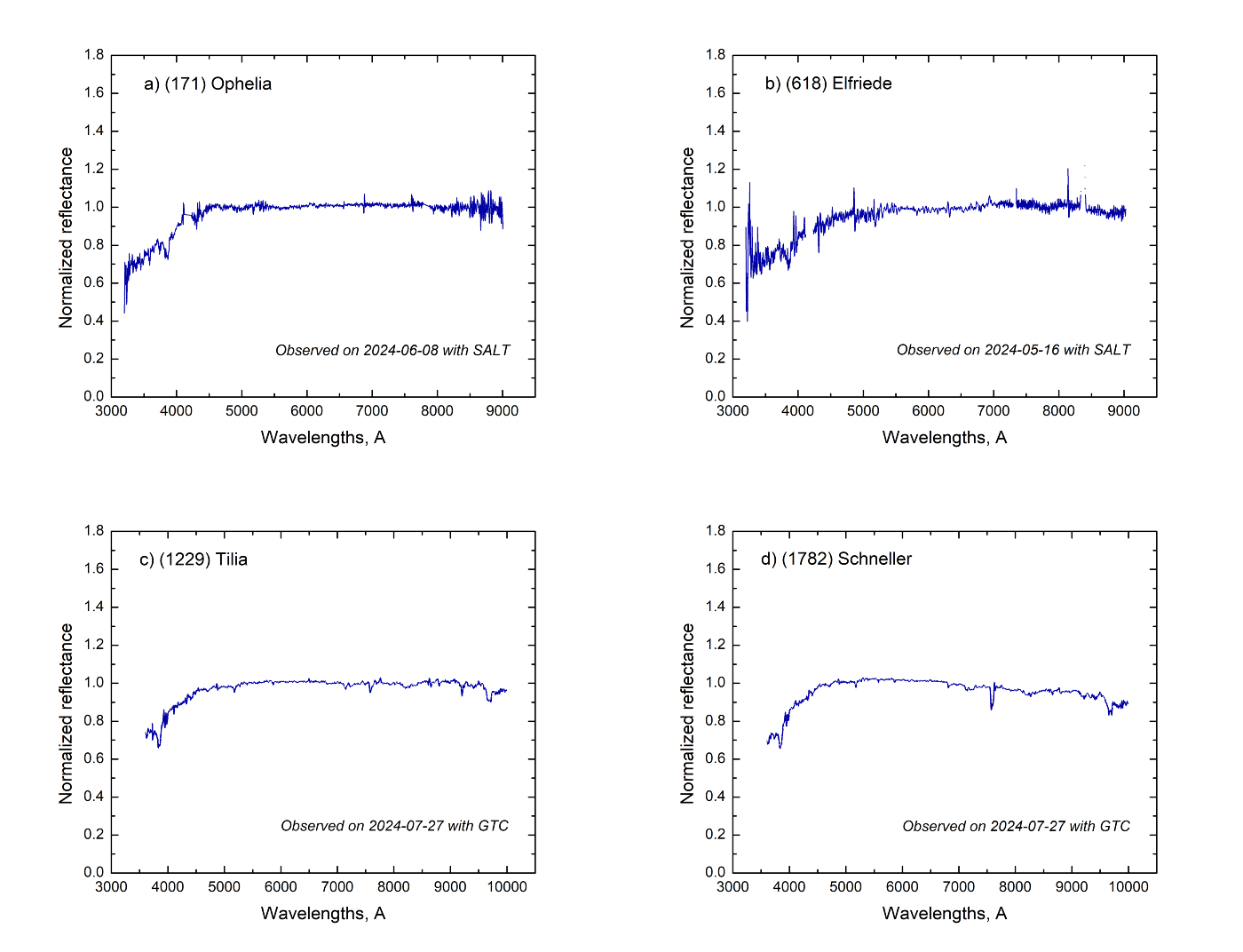
Investigation of near-ultraviolet-visible range in spectra of primitive asteroidsTue, 09 Sep, 18:00–19:30 (EEST) Finlandia Hall foyer | F113
EPSC-DPS2025-1613 | ECP | Posters | MITM8 | OPC: evaluations required
Alignment and fusion of digital terrain models : case study of planetary surfacesTue, 09 Sep, 18:00–19:30 (EEST) Finlandia Hall foyer | F109
MITM9 | Planetary in-situ measurements
EPSC-DPS2025-114 | ECP | Posters | MITM9 | OPC: evaluations required
Boulder shape analysis: is a 2D projection reliable for capturing the 3D geometry?Tue, 09 Sep, 18:00–19:30 (EEST) Finlandia Hall foyer | F115


EPSC-DPS2025-1741 | ECP | Posters | MITM9 | OPC: evaluations required
Spacecraft charging during the 2024 Juice Earth gravity assistTue, 09 Sep, 18:00–19:30 (EEST) Finlandia Hall foyer | F122
MITM10 | Laboratory experiments in support of ground observations and space missions (sample return, analogs, analytical workflow etc.)
EPSC-DPS2025-1534 | Posters | MITM10 | OPC: evaluations required
Spectral analysis of silicate glasses analog of Mercury’s geochemical terrains and comparison with MESSENGER and BepiColombo dataTue, 09 Sep, 18:00–19:30 (EEST) Finlandia Hall foyer | F129

MITM14 | Exploiting Gaia to study minor bodies of the Solar System: results, challenges, and perspectives
EPSC-DPS2025-42 | ECP | Posters | MITM14
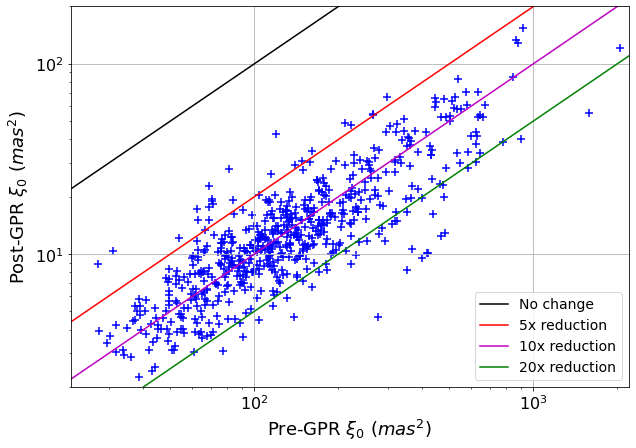
Using Gaia to reduce atmospheric turbulence displacements in LSST minor planet astrometryThu, 11 Sep, 18:00–19:30 (EEST) Finlandia Hall foyer | F99

EPSC-DPS2025-296 | ECP | Posters | MITM14 | OPC: evaluations required
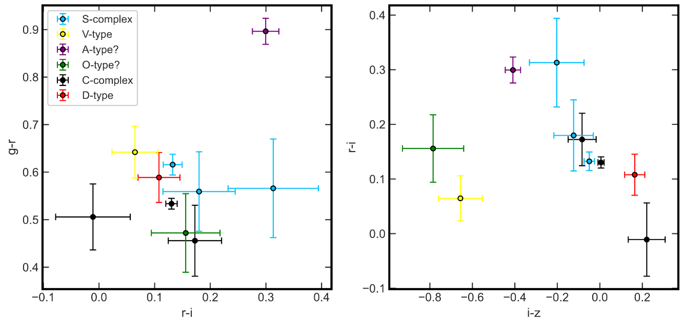
Spectral classification of Gaia DR3 Solar System small bodies and application to the search for A-type olivine-rich asteroidsThu, 11 Sep, 18:00–19:30 (EEST) Finlandia Hall foyer | F103
MITM15 | Solar System Science from JWST
EPSC-DPS2025-359 | ECP | Posters | MITM15 | OPC: evaluations required
Composition of asteroid 84 Klio with NIRSpec/JWSTThu, 11 Sep, 18:00–19:30 (EEST) Finlandia Hall foyer | F118
EPSC-DPS2025-622 | Posters | MITM15 | OPC: evaluations required
Thermodynamic modeling of metamorphic fluids supports internal source of carbon-bearing molecules at the surface of TNOsThu, 11 Sep, 18:00–19:30 (EEST) Finlandia Hall foyer | F108
EPSC-DPS2025-805 | ECP | Posters | MITM15 | OPC: evaluations required
A Scorched Story: JWST Reveals Phaethon's Dehydrated Surface Composition and Thermal HistoryThu, 11 Sep, 18:00–19:30 (EEST) Finlandia Hall foyer | F110
EPSC-DPS2025-820 | ECP | Posters | MITM15 | OPC: evaluations required
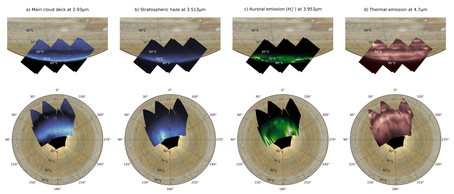
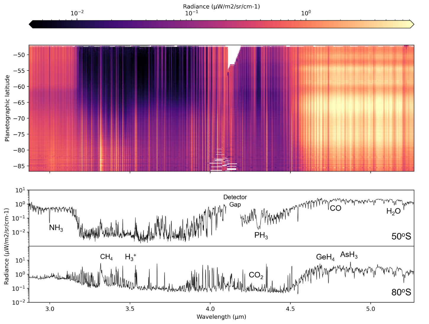
JWST/NIRSpec IFU Observations of Jupiter’s South Pole: Vertical and Latitudinal Structure of Aerosols in the Near-InfraredThu, 11 Sep, 18:00–19:30 (EEST) Finlandia Hall foyer | F111
EPSC-DPS2025-1004 | ECP | Posters | MITM15
(163) Erigone, (302) Clarissa, and (752) Sulamitis as seen with JWST’s NIRSpecThu, 11 Sep, 18:00–19:30 (EEST) Finlandia Hall foyer | F122
MITM18 | Planetary Defense: space missions, observations, modeling and experiments
EPSC-DPS2025-1400 | ECP | Posters | MITM18 | OPC: evaluations required
In-flight observations during the cruise phase of HyperScout-H instrument of ESA/Hera missionMon, 08 Sep, 18:00–19:30 (EEST) Finlandia Hall foyer | F109
SB0 | Small Body Dynamics
EPSC-DPS2025-946 | Posters | SB0
The properties of the (617) Patroclus binary system derived from the mutualevents of 2017–2018 and 2024–2025Thu, 11 Sep, 18:00–19:30 (EEST) Finlandia Hall foyer | F137
EPSC-DPS2025-1110 | ECP | Posters | SB0 | OPC: evaluations required
On the forced planes of the Hilda asteroids and other resonant groupsThu, 11 Sep, 18:00–19:30 (EEST) Finlandia Hall foyer | F132
EPSC-DPS2025-1589 | ECP | Posters | SB0
Charging and Dynamics of Interstellar Dust throughout the HeliosphereThu, 11 Sep, 18:00–19:30 (EEST) Finlandia Hall foyer | F139
EPSC-DPS2025-2091 | ECP | Posters | SB0 | OPC: evaluations required
Dynamical Evolution of Refractory Elements in an alpha-Protoplanetary DiskThu, 11 Sep, 18:00–19:30 (EEST) Finlandia Hall foyer | F135
SB3 | Observational investigations of comets
EPSC-DPS2025-869 | ECP | Posters | SB3 | OPC: evaluations required
JFC Reflectivity Reassessed: Preliminary Albedos and Statistical TrendsThu, 11 Sep, 18:00–19:30 (EEST) Finlandia Hall foyer | F148
EPSC-DPS2025-1175 | ECP | Posters | SB3
Unveiling Comet Nuclei Surface Spectra: Validating a Coma Subtraction Technique for IFU Comet ObservationsThu, 11 Sep, 18:00–19:30 (EEST) Finlandia Hall foyer | F151
EPSC-DPS2025-1182 | ECP | Posters | SB3
Spatial intensity profiles of forbidden atomic oxygen emission lines in C/2023 A3 (Tsuchinshan-ATLAS)Thu, 11 Sep, 18:00–19:30 (EEST) Finlandia Hall foyer | F163
EPSC-DPS2025-1523 | ECP | Posters | SB3
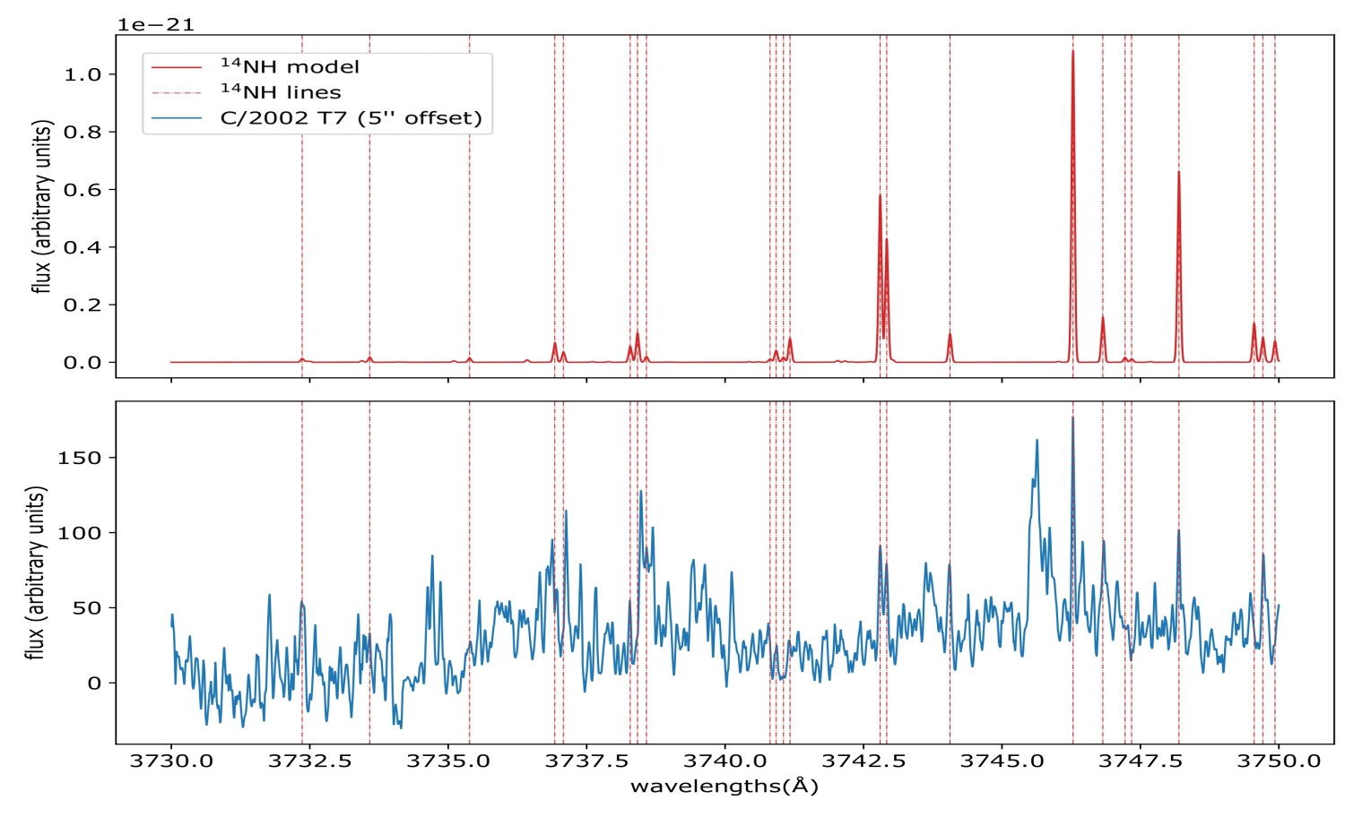
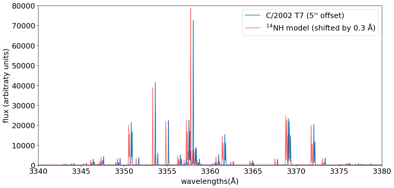
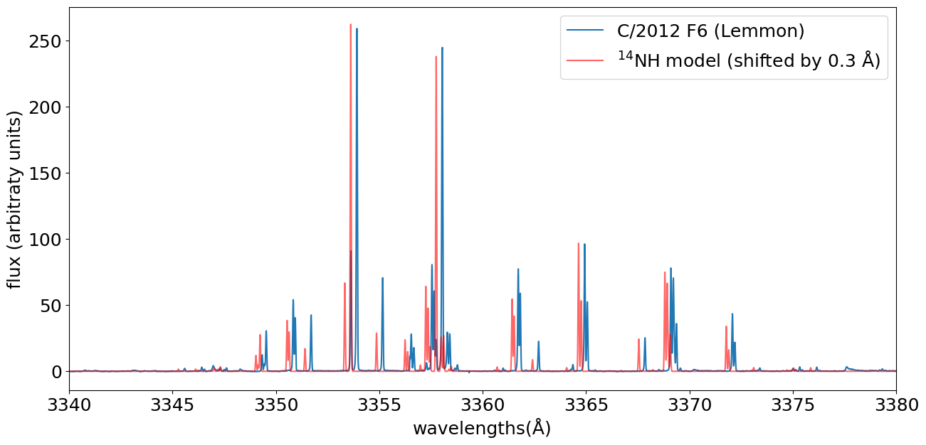
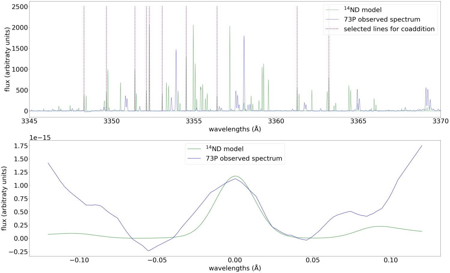
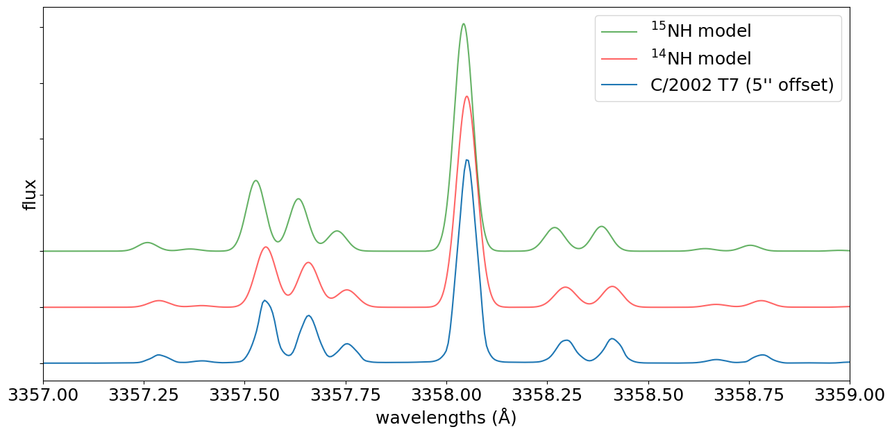
NH fluorescence models for measuring cometary D/H isotopic ratiosThu, 11 Sep, 18:00–19:30 (EEST) Finlandia Hall foyer | F155
EPSC-DPS2025-1635 | ECP | Posters | SB3
Tracing Asymmetries in the 67P’s Dust Coma Brightness Distribution Using Rosetta’s OSIRIS ObservationsThu, 11 Sep, 18:00–19:30 (EEST) Finlandia Hall foyer | F145
SB4 | Sample Return: in-progress analyses and perspectives
EPSC-DPS2025-548 | ECP | Posters | SB4
Spectral Variability and Compositional Insights from Asteroid (101955) Bennu’s Sampling Sites Using OTES DataMon, 08 Sep, 18:00–19:30 (EEST) Finlandia Hall foyer | F138


EPSC-DPS2025-1487 | ECP | Posters | SB4
3D Detection and Analysis of Lithologies in Ryugu: Insights into its Complex Geological FormationMon, 08 Sep, 18:00–19:30 (EEST) Finlandia Hall foyer | F141
SB5 | Physical properties and composition of TNOs and Centaurs
EPSC-DPS2025-227 | ECP | Posters | SB5
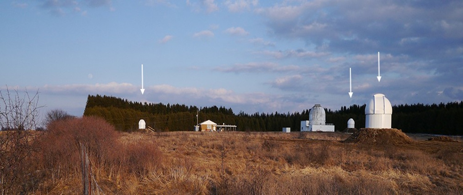
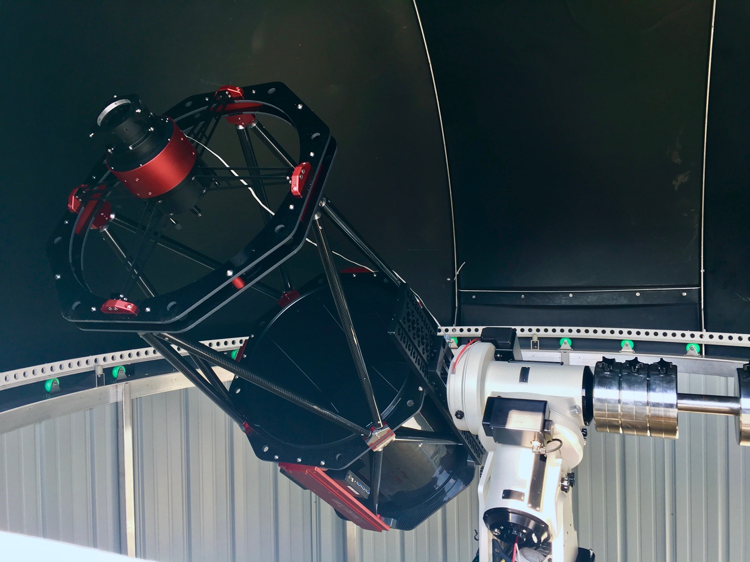
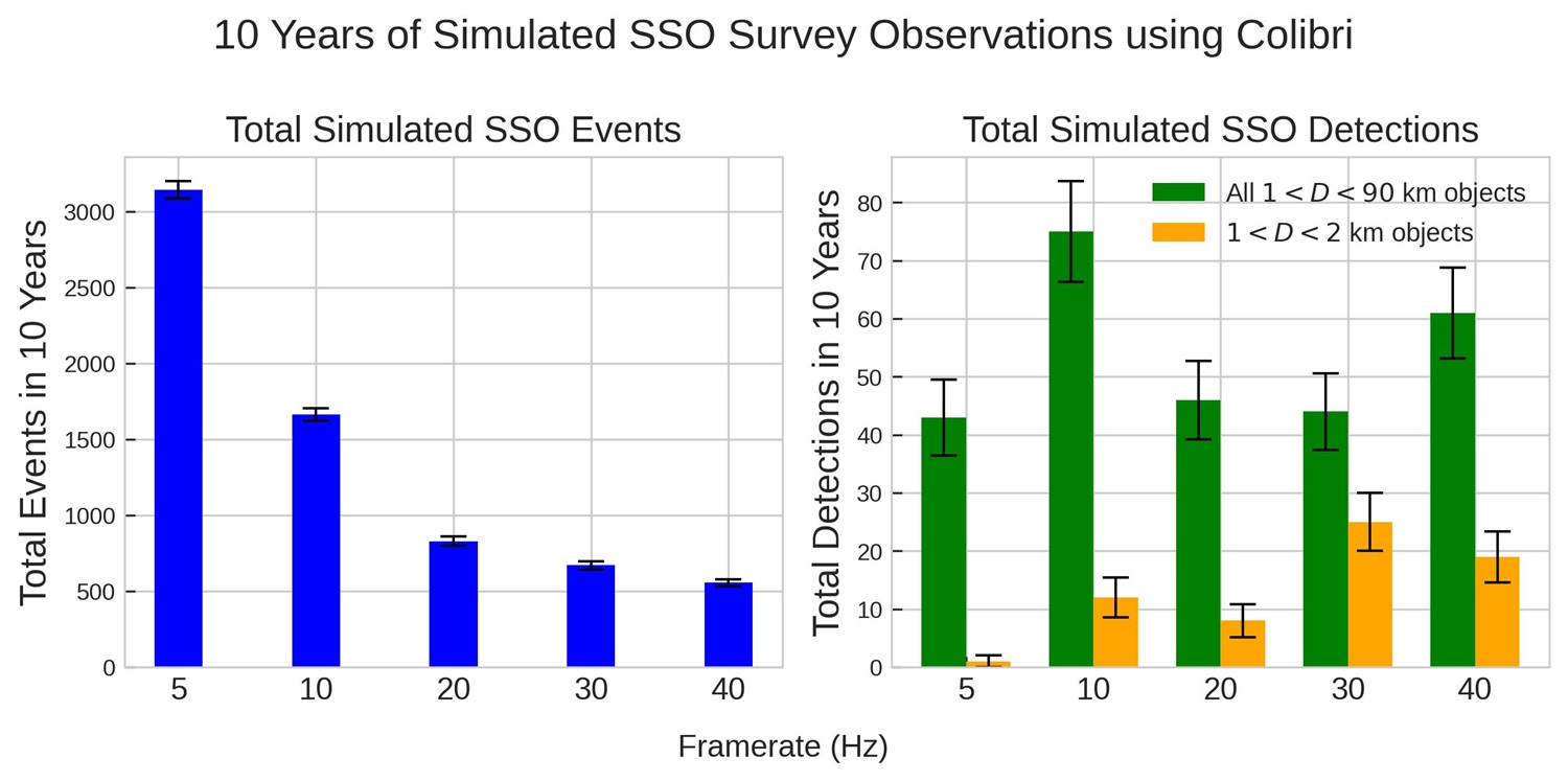
The Colibri Telescope Array for TNO Detection through Serendipitous Stellar Occultations: Simulation of Scientific PerformanceTue, 09 Sep, 18:00–19:30 (EEST) Finlandia Hall foyer | F142
EPSC-DPS2025-422 | Posters | SB5
Looking for slow objects in the outer solar systemTue, 09 Sep, 18:00–19:30 (EEST) Finlandia Hall foyer | F148
SB6 | Surface and interiors of small bodies, meteorite parent bodies, and icy moons: thermal properties, evolution, and structure
EPSC-DPS2025-134 | ECP | Posters | SB6
Thermal State and Physical Properties of Water Ice in Ceres' Oxo Crater: Implications for Surface geomorphology and EvolutionTue, 09 Sep, 18:00–19:30 (EEST) Finlandia Hall foyer | F153
EPSC-DPS2025-312 | Posters | SB6 | OPC: evaluations required
On the cohesion of the TNO Arrokoth across different density rangesTue, 09 Sep, 18:00–19:30 (EEST) Finlandia Hall foyer | F155


EPSC-DPS2025-750 | ECP | Posters | SB6
Analysis of thermalcentre-barycentre offsets and application to ALMA observationsTue, 09 Sep, 18:00–19:30 (EEST) Finlandia Hall foyer | F157
EPSC-DPS2025-1161 | ECP | Posters | SB6
Boulder Mobility on Comets: Insights from Rosetta Observations and Numerical ModellingTue, 09 Sep, 18:00–19:30 (EEST) Finlandia Hall foyer | F159
EPSC-DPS2025-1200 | Posters | SB6
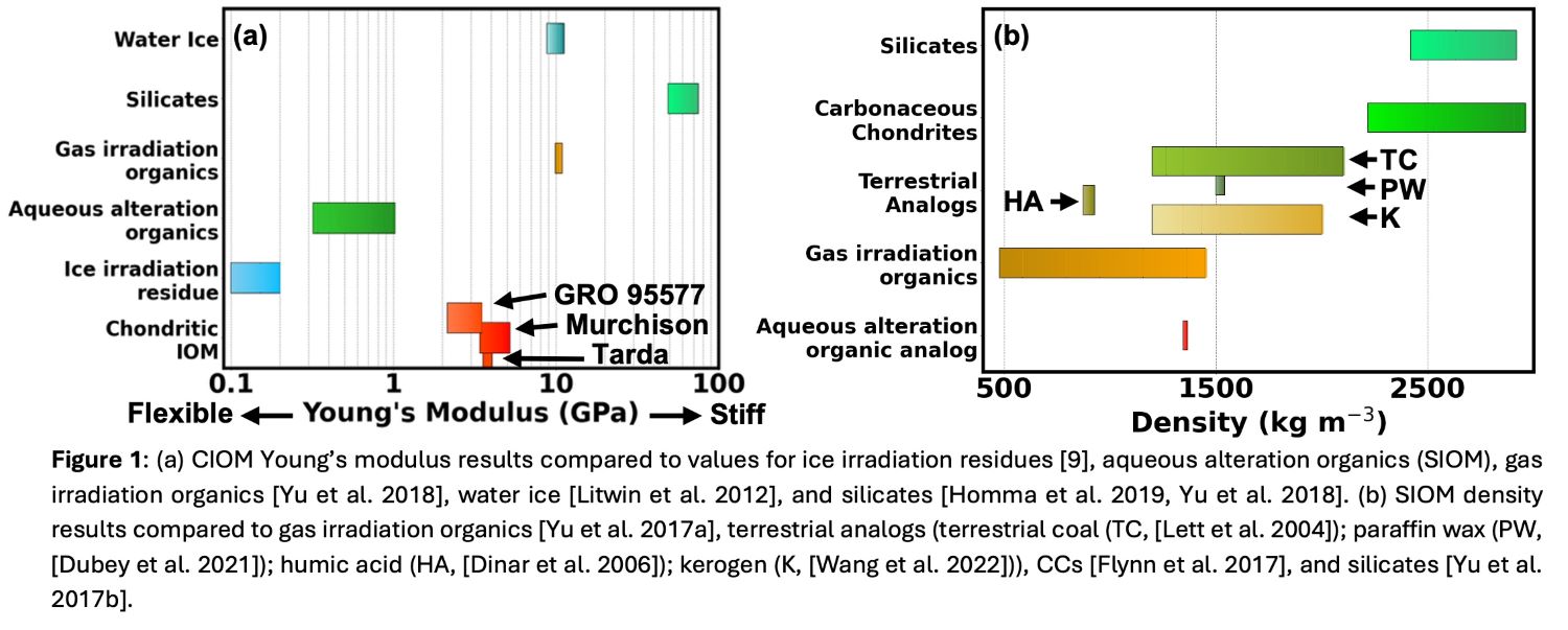
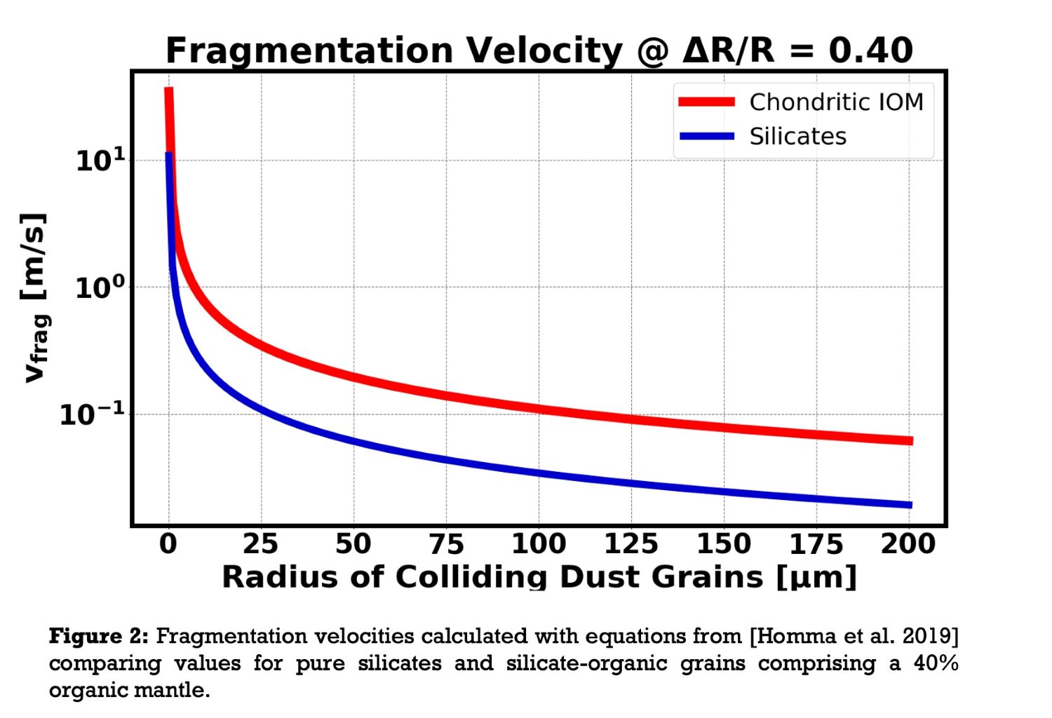
Mechanical Properties of Insoluble Organic Matter and Implications for Its Evolution and Influence on Planetary Processes.Tue, 09 Sep, 18:00–19:30 (EEST) Finlandia Hall foyer | F169
EPSC-DPS2025-1591 | ECP | Posters | SB6
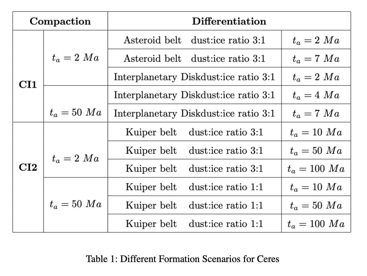
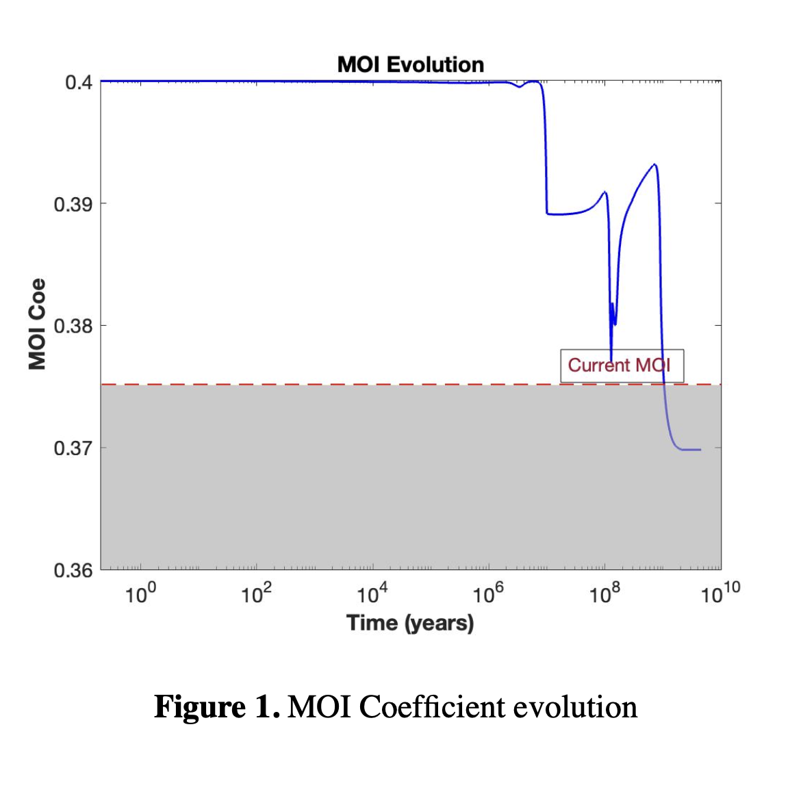
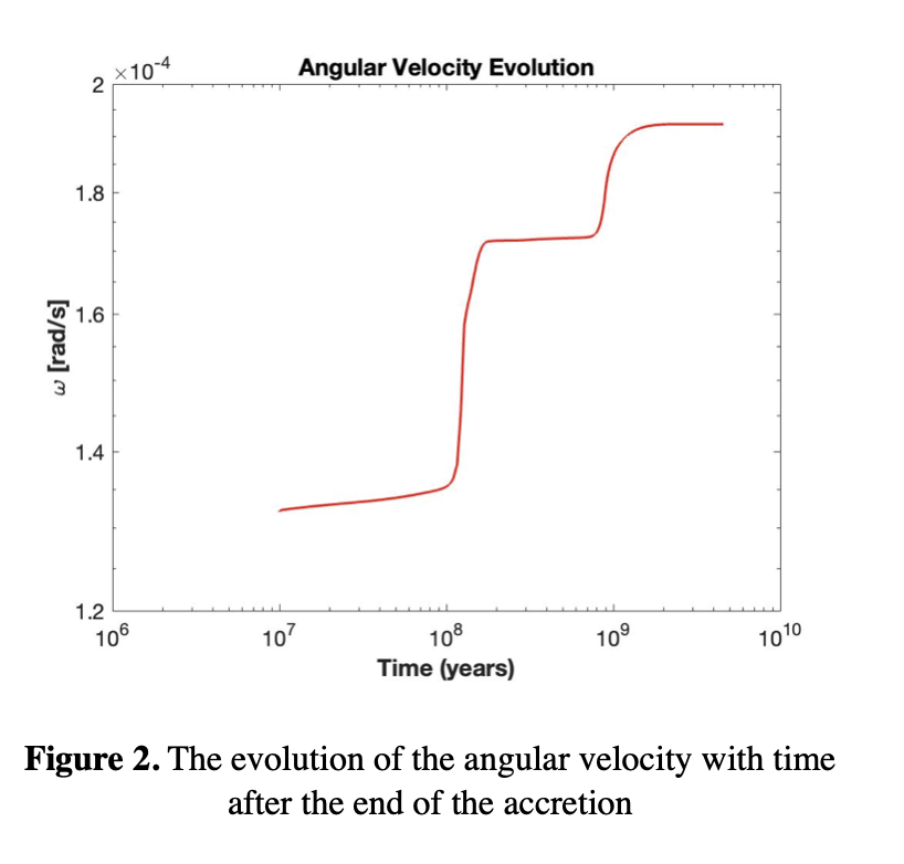
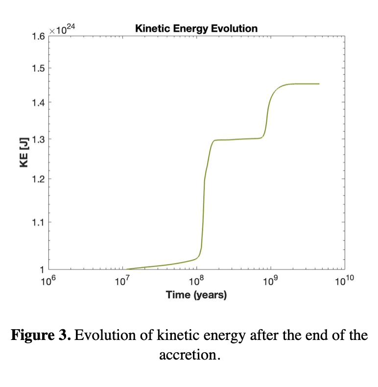
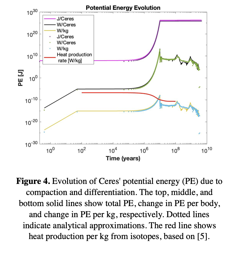
Internal Structure and Dynamical Evolution of CeresTue, 09 Sep, 18:00–19:30 (EEST) Finlandia Hall foyer | F164
EPSC-DPS2025-1966 | ECP | Posters | SB6 | OPC: evaluations required
Search for Stable Orbits around Saturn’s Moon Enceladus using Numerical ModelingTue, 09 Sep, 18:00–19:30 (EEST) Finlandia Hall foyer | F167
SB7 | Advances in Photopolarimetry and Spectropolarimetry of Solar System Small Bodies
EPSC-DPS2025-1126 | ECP | Posters | SB7
Calibration of Danuri/Wide-Angle Polarimetric Camera (PolCam): Preliminary ResultsMon, 08 Sep, 18:00–19:30 (EEST) Finlandia Hall foyer | F152
SB8 | Active small bodies: dynamics, activity, and genetic links
EPSC-DPS2025-858 | ECP | Posters | SB8 | OPC: evaluations required
RESTing Comets: Studying Dormant Comets via a Remnant Emission Survey ToolTue, 09 Sep, 18:00–19:30 (EEST) Finlandia Hall foyer | F192
EPSC-DPS2025-975 | ECP | Posters | SB8
JWST Observations of the Active Centaur 423P/Lemmon: Gas and Dust Comae CharacterizationsTue, 09 Sep, 18:00–19:30 (EEST) Finlandia Hall foyer | F193
EPSC-DPS2025-1784 | ECP | Posters | SB8 | OPC: evaluations required
N-Body Simulations of two Dynamically New Comets with different compositional characteristicsTue, 09 Sep, 18:00–19:30 (EEST) Finlandia Hall foyer | F195


SB10 | Observing and modelling meteors in planetary atmospheres
EPSC-DPS2025-976 | ECP | Posters | SB10 | OPC: evaluations required
Semi-Automated Fragmentation Modeling of Jovian ImpactsMon, 08 Sep, 18:00–19:30 (EEST) Finlandia Hall foyer | F161
EPSC-DPS2025-1320 | ECP | Posters | SB10
Metal rich cosmic spherules from Calama (Atacama Desert) and Walnumfjellet (Antarctica): a textural, chemical and isotopic comparisonMon, 08 Sep, 18:00–19:30 (EEST) Finlandia Hall foyer | F164
EPSC-DPS2025-1406 | ECP | Posters | SB10
Characterization of micrometerorites from Roysane and Nils Larsen, Sør Rondane Mountains (East Antarctica)Mon, 08 Sep, 18:00–19:30 (EEST) Finlandia Hall foyer | F166
EPSC-DPS2025-1425 | ECP | Posters | SB10
Micrometeorites from Rhodes Bluff, West AntarcticaMon, 08 Sep, 18:00–19:30 (EEST) Finlandia Hall foyer | F167
EPSC-DPS2025-1452 | ECP | Posters | SB10
Micrometeorites from western Greenland: extending micrometeorite collections to sediment traps in the northern hemisphere.Mon, 08 Sep, 18:00–19:30 (EEST) Finlandia Hall foyer | F168
EPSC-DPS2025-1734 | ECP | Posters | SB10 | OPC: evaluations required
Non destructive methodology to study GRO 95517 antarctic meteoriteMon, 08 Sep, 18:00–19:30 (EEST) Finlandia Hall foyer | F163
SB11 | The Rubin Observatory Census of the Solar System: Initial Commissioning Results and First Year Science Expectations for the Legacy Survey of Space and Time
EPSC-DPS2025-1056 | ECP | Posters | SB11 | OPC: evaluations required
Assessment of HelioLinC3D performance for near-Earth Asteroid discovery on LSST predictionsTue, 09 Sep, 18:00–19:30 (EEST) Finlandia Hall foyer | F198
SB12 | Exploring the Martian Moons: unraveling the origins of Phobos and Deimos
EPSC-DPS2025-623 | ECP | Posters | SB12
Experimental investigations of the photometric properties of Phobos simulantThu, 11 Sep, 18:00–19:30 (EEST) Finlandia Hall foyer | F168
SB15 | Computational and experimental astrophysics of small bodies and planets
EPSC-DPS2025-321 | Posters | SB15 | OPC: evaluations required
Unveiling Hidden Structures in the Main Belt: A Probabilistic Framework for Asteroid FamiliesMon, 08 Sep, 18:00–19:30 (EEST) Finlandia Hall foyer | F182
EPSC-DPS2025-332 | ECP | Posters | SB15
Hunting for Sub-Moons: A Map of Stability in the Jovian and Kronian SystemsMon, 08 Sep, 18:00–19:30 (EEST) Finlandia Hall foyer | F171
EPSC-DPS2025-726 | ECP | Posters | SB15 | OPC: evaluations required
Timescales for Hypervolatile Depletion from Small Kuiper Belt ObjectsMon, 08 Sep, 18:00–19:30 (EEST) Finlandia Hall foyer | F180
EPSC-DPS2025-958 | Posters | SB15
Ionizing atmospheres in collisions of grainsMon, 08 Sep, 18:00–19:30 (EEST) Finlandia Hall foyer | F174
EPSC-DPS2025-1558 | ECP | Posters | SB15
Resonant Dynamics and Particle Trapping Around Non-Symmetric AsteroidsMon, 08 Sep, 18:00–19:30 (EEST) Finlandia Hall foyer | F185
SB22 | Understanding the internal structure of kilometric-size asteroids through measurements and modeling
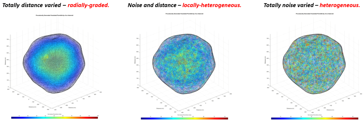
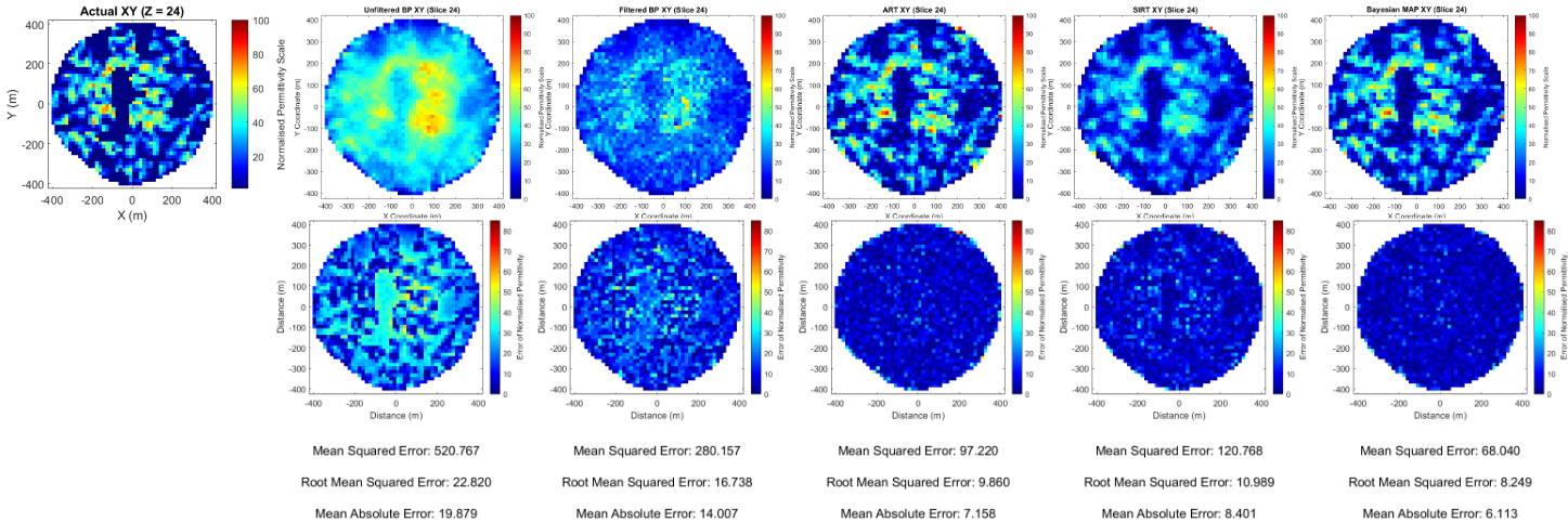
EPSC-DPS2025-831 | ECP | Posters | SB22 | OPC: evaluations required
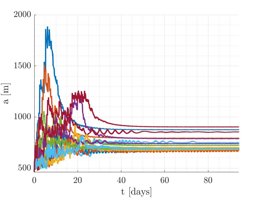
Comparative Evaluation of Inversion Methods for In-Situ RF Tomography of Kilometre-Scale AsteroidsTue, 09 Sep, 18:00–19:30 (EEST) Finlandia Hall foyer | F209
EPSC-DPS2025-871 | ECP | Posters | SB22 | OPC: evaluations required
A Preliminary Study of a Dynamical System Approach to Asteroid Gravity Inversion for Interior EstimationTue, 09 Sep, 18:00–19:30 (EEST) Finlandia Hall foyer | F211
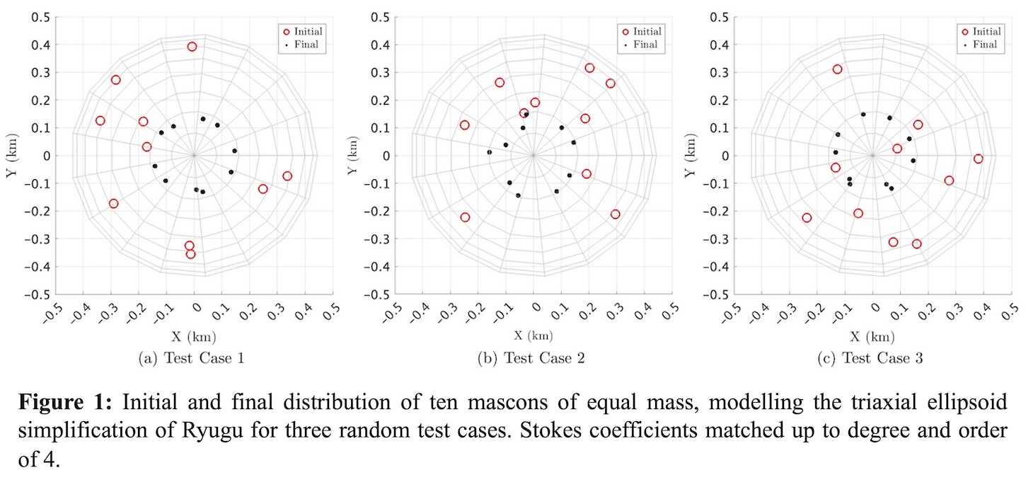

EPSC-DPS2025-1359 | ECP | Posters | SB22
Asteroid internal structure determination from Hera missionTue, 09 Sep, 18:00–19:30 (EEST) Finlandia Hall foyer | F207
EXOA0 | General Session of EXOA
EPSC-DPS2025-137 | ECP | Posters | EXOA0
Correcting for the impact of starspot-crossing events on the exoplanet transit depth with multiwavelength transit observations of CoRoT-2 bMon, 08 Sep, 18:00–19:30 (EEST) Finlandia Hall foyer | F195
EPSC-DPS2025-1541 | Posters | EXOA0
The Origin of Hot Jupiters Revealed Through Their Age DistributionMon, 08 Sep, 18:00–19:30 (EEST) Finlandia Hall foyer | F202
EPSC-DPS2025-1693 | ECP | Posters | EXOA0
Reconstructing exoplanet surfaces from unresolved light curvesMon, 08 Sep, 18:00–19:30 (EEST) Finlandia Hall foyer | F203
EXOA7 | Astrobiology
EPSC-DPS2025-121 | ECP | Posters | EXOA7 | OPC: evaluations required
Bioenergetic Modeling of Methanogens in Europa's Subsurface Ocean EnvironmentTue, 09 Sep, 18:00–19:30 (EEST) Finlandia Hall foyer | F213
EPSC-DPS2025-1237 | ECP | Posters | EXOA7
Biomolecule Remote Sensing Using Terahertz SpectroscopyTue, 09 Sep, 18:00–19:30 (EEST) Finlandia Hall foyer | F216
EXOA8 | Future and current instruments to detect and characterise extrasolar planets and their environment
EPSC-DPS2025-127 | ECP | Posters | EXOA8
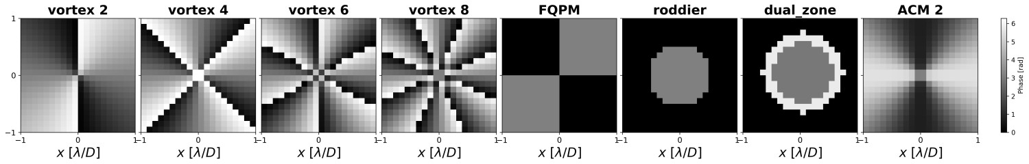
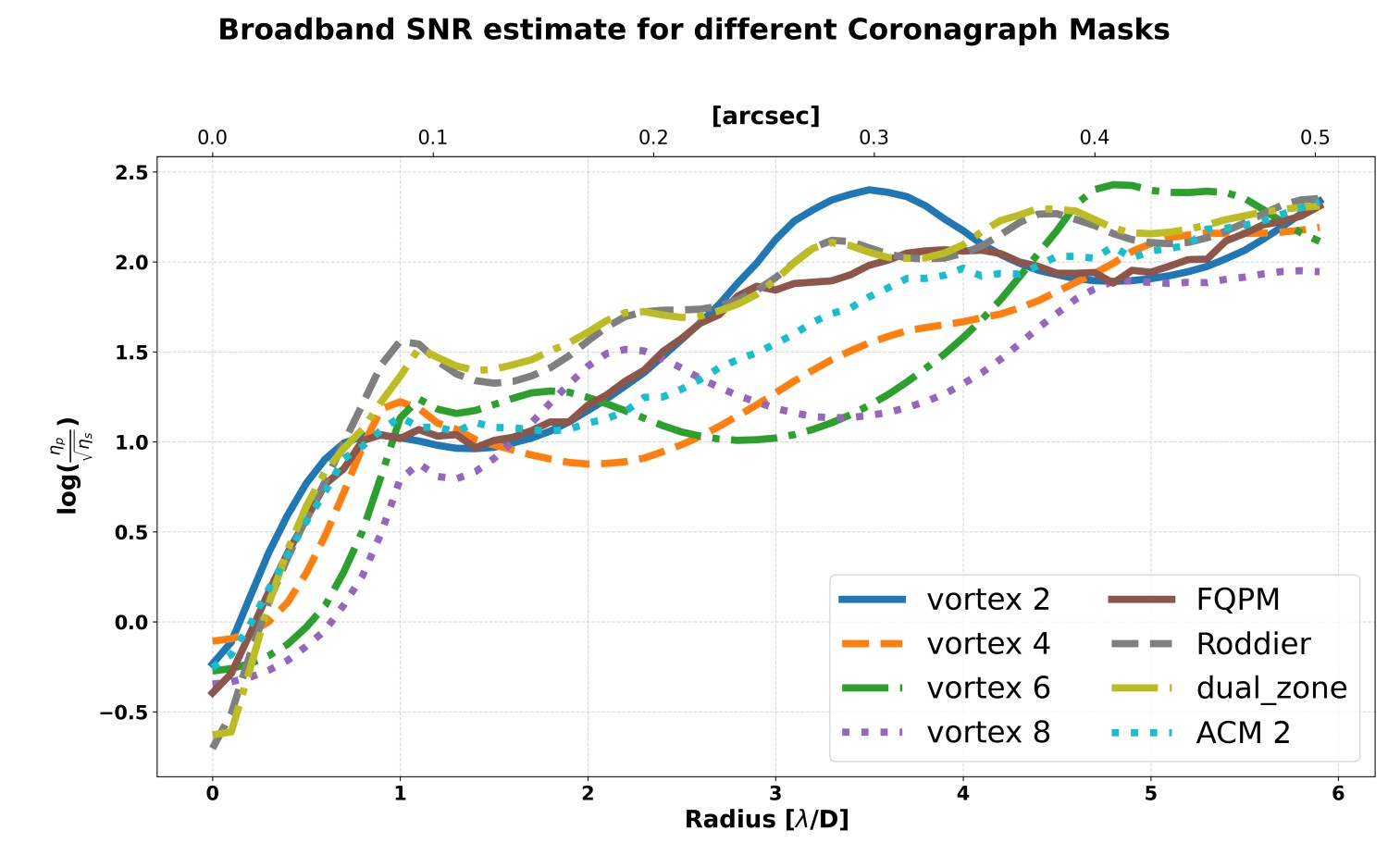
Simulating Pixelated Focal-Plane Phase Masks for Coronagraphic High-Contrast ImagingThu, 11 Sep, 18:00–19:30 (EEST) Finlandia Hall foyer | F191
EXOA11 | Exoplanet characterization of (super-)Earths and sub-Neptunes
EPSC-DPS2025-212 | ECP | Posters | EXOA11
A General Evolution Inference Framework for Close-In Small Planet PopulationsTue, 09 Sep, 18:00–19:30 (EEST) Finlandia Hall foyer | F226
EPSC-DPS2025-998 | ECP | Posters | EXOA11
Assessing the Impact of Varying HSO and HNO Cross-Sections on Photochemical Models: Implications for Spectral Characterization of Terrestrial ExoplanetsTue, 09 Sep, 18:00–19:30 (EEST) Finlandia Hall foyer | F227
EPSC-DPS2025-1521 | ECP | Posters | EXOA11
Exploring the Atmosphere of K2-18b through Retrievals and Forward ModellingTue, 09 Sep, 18:00–19:30 (EEST) Finlandia Hall foyer | F231
EXOA12 | Planet formation and evolution in solar system analogs
EPSC-DPS2025-636 | ECP | Posters | EXOA12
Planetesimal formation: On the evolution of super strong charge spots from colliding grainsThu, 11 Sep, 18:00–19:30 (EEST) Finlandia Hall foyer | F203
EPSC-DPS2025-1202 | ECP | Posters | EXOA12
Global N-body simulation of planetary formation: The origins of Ice giantsThu, 11 Sep, 18:00–19:30 (EEST) Finlandia Hall foyer | F205
EXOA15 | Recasting the Cosmic Shoreline in light of JWST: The Fate of Rocky Exoplanet Atmospheres
EPSC-DPS2025-1756 | ECP | Posters | EXOA15
Refining Exoplanet Escape Predictions with Molecular-Kinetic SimulationsThu, 11 Sep, 18:00–19:30 (EEST) Finlandia Hall foyer | F221
EXOA18 | Investigating Habitability and Biosignatures within Exoplanet Atmospheres
EPSC-DPS2025-98 | ECP | Posters | EXOA18
Habitability on exoplanets in eccentric orbits: the case of Gl 514 b and HD 20794 dThu, 11 Sep, 18:00–19:30 (EEST) Finlandia Hall foyer | F232


EXOA19 | AI for exoplanet and brown dwarf studies
EPSC-DPS2025-93 | Posters | EXOA19
Abstract: Can Gaia combined with AI help-us plant seeds in the Brown-Dwarf desert?Mon, 08 Sep, 18:00–19:30 (EEST) Finlandia Hall foyer | F211
EPSC-DPS2025-542 | ECP | Posters | EXOA19 | OPC: evaluations required
Multi-method extraction of quasi-periodic exoplanet signals from noisy data in transit surveysMon, 08 Sep, 18:00–19:30 (EEST) Finlandia Hall foyer | F214